CS 484: Computational Vision
Yuri Boykov
Estimated study time: 6 hr 2 min
Table of contents
Introduction to Computational Vision
What Is Computer Vision?
Human vision begins when light reflected from objects reaches the eye’s photoreceptors, producing signals that travel to the brain, which interprets the scene — inferring a garden, a bridge, the geometry of 3D space, the identities of objects, and their spatial relationships. Computer vision asks: can we build machines that replicate this interpretive process? The sensor is no longer a biological eye but a grid of electronic sensing elements arranged on an image plane inside a camera. The signals those elements produce — a rectangular array of intensity values — are then analysed by algorithms that attempt to recover scene understanding from raw pixel data.
Computer Vision and Its Relationship to Computer Graphics
Computer graphics and computer vision are, in a meaningful sense, inverses of each other. Graphics starts from a computer model — geometry, materials, lighting — and renders it into an image. Vision starts from an image and attempts to recover the underlying model: shapes, lighting, motion, object identities. Both fields share a substantial intersection in modelling, where the representation of 3D shape, surface properties, and illumination is central. Vision draws further on detection, tracking, motion estimation, and recognition, while graphics focuses on surface design, animation, and user interfaces for controlling rendered scenes.
An Interdisciplinary Field
Computational vision sits at the intersection of many disciplines. Biology and neuroscience inform our understanding of how living organisms perceive visual scenes, motivating both the problems we study and some of the algorithmic approaches we take. Physics underlies the formation of images — how light travels, reflects, and refracts. Mathematics — particularly linear algebra, probability, optimization, and geometry — provides the formal backbone of virtually every algorithm in the field. Psychology and cognitive science shed light on how perception and attention operate in humans. Machine learning has become the dominant paradigm for learning visual representations from data. Robotics provides some of the most demanding application contexts, while medical imaging connects the field to engineering and clinical practice.
The goal of computational vision, stated simply, is to bridge the gap between pixels and meaning. A computer sees only a two-dimensional table of numbers. The task of the vision system is to infer from those numbers the rich semantic content that a human perceives immediately and effortlessly.
Applications of Computer Vision
Optical Character Recognition
One of the earliest successful applications, optical character recognition (OCR) allows computers to read printed or handwritten text. Reliable systems for printed text were available by the early 1990s and are now ubiquitous in postal sorting, document scanning, and mobile applications.
Object Detection and Tracking
Object detection is the task of locating instances of specific object categories within an image, typically by predicting bounding boxes. Face detection became practical around 2000 using methods such as the Viola-Jones cascade classifier, and modern deep-learning detectors can localise hundreds of object categories simultaneously in real time. Tracking extends detection across time, maintaining the identity of objects across video frames. Methods such as pictorial structures decompose articulated objects into parts with spatial constraints, enabling tracking of human body configurations across a sequence.
Segmentation
Segmentation is the problem of assigning a label to every pixel in an image, producing a pixel-accurate partitioning of the scene. Early energy minimisation methods — Livewire (1995) and graph cuts (2001–2004) — enabled interactive segmentation tools in which a user sketches a rough outline and the algorithm snaps to precise object boundaries. These methods found rapid adoption in medical image segmentation, where graph-cut techniques enabled reliable 3D organ extraction from CT volumes as early as 2001. Later, combining detection with segmentation led to panoptic segmentation systems (exemplified by the CityScapes dataset) that simultaneously identify object instances and label every pixel with a semantic category.
Activity Recognition
Activity recognition systems interpret the temporal structure of video, identifying human actions such as walking, running, or gesturing. Bottom-up tracking methods that aggregate motion evidence across frames provide the foundation for such recognition pipelines.
Vision-Based Interaction and Assistive Technology
The Microsoft Kinect (2010) brought structured-light 3D sensing to consumer hardware, enabling markerless body tracking for gaming. The same depth-sensing technology underpins assistive technologies that help people with mobility impairments interact with computers and environments through gesture.
Stereo and Multi-View Reconstruction
Humans perceive depth partly because our two eyes observe the world from slightly different positions — the disparity between the two views provides a powerful depth cue. Stereo reconstruction algorithms recover a dense depth map from pairs of calibrated images; competitive results were demonstrated as early as 1999. By 2005, systems using many images from different viewpoints were producing full 3D surface models. Structure from Motion (SfM) methods take an unordered collection of photographs and simultaneously recover camera positions and a sparse 3D point cloud, enabling the reconstruction of large scenes from casual photography.
3D Scene Reconstruction
Beyond stereo, scenes can be reconstructed from point clouds obtained by laser scanners using surface-fitting algorithms. Impressive results from just a handful of images were achieved by Debevec, Taylor, and Malik at SIGGRAPH 1996. More remarkably, monocular depth estimation — recovering depth from a single image — has become possible through learning. Godard et al. (CVPR 2017) demonstrated that a neural network trained on stereo pairs can predict plausible depth maps at test time from a single photograph, exploiting learned priors about scene geometry.
Vision for Robotics
NASA’s Mars Exploration Rover Spirit used an onboard vision system to navigate hostile terrain autonomously. The system solved multiple simultaneous tasks: panorama stitching of wide-angle imagery, 3D terrain modelling to identify safe traversal paths, position tracking to maintain localisation without GPS, and obstacle detection to avoid rocks and craters. This application illustrates how computer vision underpins autonomous systems that must operate far beyond the reach of direct human control.
Image Modalities
Part I: Photo and Video Data
The Pinhole Camera and Camera Obscura
To understand digital imaging, it is useful to reason from first principles about how cameras form images. Consider the simplest possible “camera”: a piece of film placed directly in front of a scene. Every point on the film receives light from every visible point in the scene simultaneously, so the film records a completely blurred superposition of the entire scene — no useful image is formed.
The key insight behind the Camera Obscura (Latin: dark room), known to Aristotle and described in detail by Athanasius Kircher in 1646, is that introducing a barrier with a small hole dramatically improves image formation. Most rays from each scene point are blocked; only the ray passing through the hole reaches the film. The result is a dim but spatially coherent image, with the depth of the room corresponding to the focal length of the device. The pencil of rays — all rays passing through the aperture from a single point — converges on the film to produce a sharp pixel, as long as the aperture is small enough.
This principle carries a fundamental consequence. Because 3D space is projected onto a 2D image plane, depth information is lost: a nearby small object and a distant large object can produce identical images. Depth is therefore inherently ambiguous in a single photograph. Recovering it requires additional information — multiple viewpoints, prior knowledge about scene geometry, or learning from data — which is a recurring theme throughout the course.
Aperture Size and Diffraction
There is a tension in pinhole camera design: making the aperture smaller sharpens the image by blocking more extraneous rays, but it also reduces the amount of light reaching the film and eventually introduces diffraction effects. When the aperture diameter becomes comparable to the wavelength of visible light (roughly 400–700 nm), the wave nature of light causes rays to spread after passing through the hole, reintroducing blur. In practice, extremely small apertures are therefore impractical.
Lenses
Lenses resolve the aperture dilemma by gathering light over a large area and refracting it so that all rays from a single scene point converge to a single image point. A lens of sufficient size can collect far more light than a pinhole while still producing a sharp image — provided the scene point lies at the correct depth. Points at other depths focus behind or in front of the image plane, producing a circle of confusion: a small disk rather than a point. Moving the image plane (changing the image distance) shifts which depths are in focus.
The focal length of a lens is defined as the image distance at which objects at infinity appear sharply focused. Focal length depends on the physical construction of the lens (the curvature of its surfaces and the refractive index of the glass). Many camera lenses are multi-element systems that allow the effective focal length to be varied (zoom lenses).
The Pinhole Camera Model
Because modelling circles of confusion and depth of field adds considerable complexity, computational vision typically adopts the simplified pinhole camera model. In this model, a single point — the optical centre \(C\), also called the viewpoint — replaces the lens, and an image plane is positioned at distance \(f\) (the focal length) in front of it. Every scene point is mapped to the image plane by the ray connecting it to \(C\). Equivalently, one can draw the image plane as a virtual plane on the same side of \(C\) as the scene (in front of the camera), which avoids the inversion inherent in a real pinhole and is the convention used throughout the course.
Projective Geometry of the Pinhole Camera
To describe the mapping from 3D scene points to 2D image pixels mathematically, we adopt a camera-centred coordinate system. The optical centre \(C\) is placed at the origin. The \(x\)- and \(y\)-axes lie parallel to the image plane, aligned with the horizontal \(u\) and vertical \(v\) axes of the image coordinate system respectively. The \(z\)-axis, called the optical axis, points forward through the centre of the image.
Under these assumptions, a 3D world point \((x, y, z)\) projects onto image pixel \((u, v)\) according to:
\[ (x,\, y,\, z) \;\longmapsto\; \left( f\,\frac{x}{z},\; f\,\frac{y}{z} \right) \]The factor \(1/z\) embodies the key perceptual fact that objects appear smaller as they recede: the apparent size of any 3D object in the image is inversely proportional to its distance \(z\) from the camera. This mapping is called a perspective projection, and it is the foundation for all the geometric reasoning covered in later lectures (warping, homographies, stereo, and multi-view geometry).
The Human Eye as a Camera
The human eye is a biological realisation of the camera principle. The iris is a coloured annulus of radial muscles that controls the pupil — the aperture through which light enters. The pupil adjusts dynamically to regulate the amount of incoming light. The lens of the eye (which can change shape to adjust focal length, a process called accommodation) focuses light onto the retina at the back of the eye. The retina is lined with photoreceptor cells: rods (sensitive to low light, monochromatic) and cones (sensitive to colour, concentrated in the fovea at the centre of the visual field). These cells play the role of the film or sensor in a camera.
Digital Image Formation
Real cameras transduce light into electrical signals using CCD or CMOS image sensors. The intensity recorded at each sensor element depends on two physical quantities:
\[ f(x, y) = \text{reflectance}(x, y) \times \text{illumination}(x, y) \]Reflectance is a material property — the fraction of incident light that the surface reflects — and lies in \([0, 1]\). Illumination is the amount of light falling on the surface from the environment and can in principle be unbounded. Their product gives the image irradiance at each point.
Sampling and Quantization
Before we can process an image on a computer, the continuous signal must be converted to a discrete array through two operations:
- Spatial sampling: The image plane is divided into a regular grid. The continuous intensity value at each grid location is measured. If the grid spacing is \(\Delta\), the sampled image is written \(f[i, j] = f(i\Delta, j\Delta)\). The density of the grid determines the spatial resolution, typically expressed in pixels.
- Intensity quantization: Each sampled intensity value is rounded to the nearest integer from a finite set. An 8-bit image stores values in \(\{0, 1, \ldots, 255\}\). The number of bits used is the bit depth (also called intensity depth or colour depth).
Increasing spatial resolution captures finer detail; increasing bit depth captures more subtle intensity gradations. Insufficient resolution causes aliasing; insufficient bit depth causes visible contouring artefacts.
Images as Functions
Mathematically, a greyscale image is a function \(f : \mathbb{R}^2 \to \mathbb{R}\), where \(f(x, y)\) gives the intensity at continuous image coordinates \((x, y)\). In practice we restrict attention to a rectangle and a bounded intensity range:
\[ f : [a,b] \times [c,d] \;\to\; [0, 1] \]A colour image is a vector-valued function with one component per colour channel. In the standard RGB representation:
\[ \mathbf{f}(x,y) = \begin{pmatrix} r(x,y) \\ g(x,y) \\ b(x,y) \end{pmatrix} \]where \(r\), \(g\), and \(b\) give the red, green, and blue channel intensities respectively.
After sampling and quantization, a digital image is represented as a 2D matrix of integers. This functional/matrix duality is central to image processing: filtering algorithms are naturally described as operations on the continuous function \(f\), but the implementation operates on the discrete matrix.
Image Data Tensors
Modern vision systems generalise the 2D image to multi-dimensional tensors:
- Colour image: A \(H \times W \times 3\) array with height \(H\), width \(W\), and 3 colour channels (RGB).
- Video: A \(H \times W \times T\) array, where \(T\) indexes frames over time. Processing video requires algorithms that exploit both spatial and temporal structure.
- Medical volumetric data: A \(H \times W \times Z\) array, where \(Z\) indexes slices along the third spatial dimension. CT and MRI scanners produce such volumes by acquiring a series of parallel 2D cross-sections.
In deep learning, images are typically represented as tensors of shape \((C, H, W)\) or \((H, W, C)\) and batched into \((N, C, H, W)\) for training.
Part II: Medical Images and Volumes
Medical imaging provides some of the most scientifically important and technically challenging applications of computer vision. Unlike natural photographs, medical images are acquired using physical phenomena other than visible-light photography, and they frequently require 3D volumetric analysis.
X-Ray Imaging
X-rays were discovered by Wilhelm Conrad Röntgen in 1895 — the “X” standing for unknown at the time — and Röntgen was awarded the first Nobel Prize in Physics in 1901 for this discovery. X-ray imaging (also known as radiography or Röntgen imaging) remained the dominant modality in medical imaging until the 1970s.
X-rays are high-energy electromagnetic radiation that penetrate soft tissue but are strongly absorbed by dense materials. Calcium in bone absorbs X-rays most strongly, producing bright white regions on a film or detector. Fat and other soft tissues absorb less, appearing in grey tones, while air absorbs almost nothing and renders as black — which is why the lungs appear dark on a chest radiograph.
Conventional X-ray imaging is fundamentally 2D projection imaging: it collapses the entire 3D body along the direction of the beam into a single 2D shadow image. Depth information along the beam axis is completely lost, though it can be partially recovered by combining images from multiple angles — the insight that eventually led to computed tomography.
Computed Tomography
The mathematical foundation for tomographic reconstruction — recovering a 2D cross-sectional image from its 1D projections — was laid by Johann Radon in 1917. The Radon transform \(g(s, \theta)\) represents the integral of a function \(f(x, y)\) along a line parameterised by offset \(s\) and angle \(\theta\). Its inversion formula (filtered backprojection) provides a practical algorithm for CT reconstruction.
The first clinical Computed Tomography (CT) scanner was developed by Godfrey Hounsfield at EMI PLC in 1972. Hounsfield shared the 1979 Nobel Prize in Physiology or Medicine with Allan Cormack, who had independently developed the mathematical theory of reconstruction. The word tomography derives from the Greek tomos (slice), reflecting the fact that CT reconstructs thin cross-sectional slices through the body rather than projections through its full depth.
The evolution of CT resolution has been remarkable: early 1970s scanners produced coarse 80×80 images with 3 mm pixels and 13 mm thick slices, requiring 80 seconds per slice. Modern multi-slice CT systems produce 512×512 images with sub-millimetre pixels and slice thicknesses below 0.5 mm, complete a full rotation in 0.5 seconds, reconstruct each slice in another 0.5 seconds, and acquire up to 16 slices simultaneously using spiral (helical) scanning. This isotropic resolution — comparable in all three spatial dimensions — enables true 3D volumetric reconstruction and multiplanar reformatting.
Despite initial scepticism (one neuroradiologist reportedly dismissed early CT images as “pretty pictures that will never replace radiographs”), CT rapidly became indispensable. It is now a cornerstone of diagnostic radiology, particularly for trauma, oncology, and neurological assessment.
Magnetic Resonance Imaging
Magnetic Resonance Imaging (MRI) exploits the quantum-mechanical property of nuclear spin. Hydrogen nuclei (protons) are abundant in biological tissue (particularly in water and fat). When placed in a strong magnetic field and excited by radiofrequency (RF) pulses, they precess at a characteristic frequency and emit a small RF signal as they return to equilibrium. Spatial encoding using magnetic field gradients allows reconstruction of a 3D image of proton density and relaxation times.
The key figures in MRI’s development were Paul Lauterbur, who demonstrated the first magnetic resonance images in Nature in 1973, and Sir Peter Mansfield, who developed the mathematics of rapid imaging sequences. Raymond Damadian built the first whole-body MRI scanner in 1977. Lauterbur and Mansfield shared the 2003 Nobel Prize in Physiology or Medicine.
Unlike CT, MRI does not use ionising radiation, making it safe for repeated examinations. It provides exceptional soft-tissue contrast, distinguishing structures that appear nearly identical on CT. The signal depends on tissue-specific relaxation times T1 and T2, which are exploited to produce different contrasts by varying the RF pulse sequence.
Advanced MRI Modalities
Beyond standard T1 and T2-weighted imaging, a range of specialised sequences have expanded MRI’s capabilities:
- Magnetic Resonance Angiography (MRA): By tuning the scanner to detect moving structures, MRA produces 3D images of blood vessels without requiring X-ray contrast agents. Gadolinium-based contrast agents can further enhance vascular conspicuity.
- Magnetic Resonance Spectroscopy (MRS): Rather than imaging anatomy, MRS measures the chemical composition of tissue — the relative concentrations of metabolites such as choline, creatine, and N-acetylaspartate. This provides information about brain chemistry and muscle metabolism that is invisible to anatomical imaging.
- Functional MRI (fMRI): Active brain regions demand increased oxygen delivery via blood flow. Oxygenated and deoxygenated haemoglobin have different magnetic properties, producing a Blood Oxygen Level-Dependent (BOLD) signal change of roughly 1%. By correlating these changes with a stimulus or task (for example, watching a flickering disk), fMRI maps brain regions involved in specific cognitive and sensory functions. It is an essential tool in both neuroscience research and pre-surgical planning.
- Diffusion-Weighted MRI (DWI) and Tractography: DWI measures the microscopic diffusion of water molecules, which in neural tissue is anisotropic — faster along the long axis of nerve fibres than perpendicular to them. Fitting a diffusion tensor to the measured diffusion in each voxel yields a field of ellipsoids encoding local fibre orientation. Tractography algorithms then trace streamlines through this field, reconstructing the large white-matter fibre tracts that connect different brain regions — results that, as one neuroanatomist observed, look “just like Gray’s Anatomy.”
- Perfusion-Weighted MRI (PWI): Measures blood flow and volume at the tissue level, important for stroke diagnosis.
Ultrasound
Ultrasound imaging uses high-frequency sound waves (typically 1–20 MHz) rather than electromagnetic radiation. A transducer emits a pulse; echoes reflected from tissue interfaces are timed to reconstruct a depth profile (A-mode) or 2D cross-section (B-mode). Ultrasound is real-time, portable, and uses no ionising radiation, making it the modality of choice for foetal imaging, cardiac assessment, and point-of-care applications. Its main limitation is poor penetration in bone and gas, and operator-dependent image quality.
Each of these modalities provides a different window into biological structure and function. Computational vision and medical image analysis draw on all of them, applying segmentation, registration, detection, and reconstruction algorithms to tasks ranging from tumour delineation to surgical guidance.
Image Pre-Processing and Low-Level Features
Overview: Low-Level Features and the Role of Filtering
Computer vision approaches the problem of image understanding at many levels of abstraction. High-level understanding concerns itself with semantic categories — what objects are present in a scene, where they are located, and what relationships exist among them. Low-level features, by contrast, operate closer to the raw signal: pixel intensities, colors, local contrast, edges, and corners. These low-level measurements are the foundation upon which all higher reasoning is built, and understanding them thoroughly is essential before tackling the more sophisticated machinery of neural networks or 3D reconstruction that appears later in the course.
The pipeline of feature extraction can be visualized as a cascade. Raw sensor output flows through a layer of low-dimensional, hand-designed low-level filters that produce filtered features — edges, corners, texture descriptors, and similar measurements. Later in the course, these hand-designed filters give way to compositions of learnable filters (deep neural networks), which produce high-dimensional features suited for semantic discrimination. Lecture 3 is concerned entirely with the first stage of this pipeline.
The mathematical apparatus central to low-level feature extraction is filtering, implemented through the operation of convolution or cross-correlation. Filtering is a form of neighborhood processing: rather than transforming each pixel in isolation, the output at any given location depends on a small spatial neighborhood around that location. This is a crucial conceptual step beyond simple point processing. As a motivating example, consider what happens when all pixels in an image are randomly shuffled: the histogram of intensities is completely unchanged, so no amount of point processing could recover the original appearance, yet any human can instantly recognize that the spatial structure — the very thing that makes the image intelligible — has been destroyed. Spatial information is indispensable, and filtering is the tool that exploits it.
Point Processing
Before neighborhood processing, the simplest form of image transformation is point processing, in which each output pixel depends only on the corresponding input pixel. Formally, if \( f \) is the original image and \( g \) the output, then
\[ g(x, y) = t(f(x, y)) \]where \( t \) is an intensity transforming function mapping the input intensity range to the output intensity range. Because every pixel is processed independently and spatial relationships play no role, point processing cannot capture or exploit any structure in the image. What it can do is globally redistribute the intensity values in useful ways.
Domain vs. Range Transformations
Image processing operations broadly fall into two families. Domain (geometric) transformations rearrange pixel locations without altering their intensities:
\[ g(x, y) = f(t_x(x, y),\; t_y(x, y)) \]where \( t_x \) and \( t_y \) are coordinate mapping functions. Flipping, rotating, or translating an image are all domain transformations. Range transformations leave positions fixed but alter intensity values, and point processing is the simplest member of this family. Filtering is a generalization of range transformations that incorporates a neighborhood of size \( \epsilon \) around each pixel:
\[ g(x, y) = \int_{|u| \le \epsilon} \int_{|v| \le \epsilon} h(u, v)\, f(x - u, y - v)\, du\, dv \]where \( h \) is the filter function. Domain transformations are the topic of the next lecture; point processing and filtering are the subjects of the present one.
Grayscale Intensity Transformations
To understand point processing concretely, consider various choices of the function \( t \) and visualize them as plots with input intensity on the horizontal axis and output intensity on the vertical axis. The identity transformation, \( t(I) = I \), leaves all intensities unchanged. The negative transformation, \( t(I) = 255 - I \), reverses the ordering of intensities so that dark regions become bright and vice versa; medical imaging sometimes employs this because certain tissue boundaries are more visible in the negative. Monotonically increasing functions that are not the identity stretch or compress different parts of the intensity range without reversing order.
Gamma Correction
A particularly important family of point-processing transforms is gamma correction, defined by
\[ t(I) = c \cdot I^{\gamma} \]where \( c \) is a scaling constant (often set to 1) and \( \gamma \) is the key parameter. When \( \gamma = 1 \) the transform is the identity. When \( \gamma > 1 \) (for example, \( \gamma = 5 \), the function effectively ignores dark input intensities and compresses them toward zero while spreading the upper range of highlights across the full output range — useful for images that are overexposed. Conversely, when \( \gamma < 1 \) (for example, \( \gamma = 0.4 \), the transform expands the lower intensity range, bringing out detail in dark regions. In practice, gamma correction is routinely applied to compensate for camera acquisition artifacts such as over- or underexposure. An overexposed image has almost all pixels concentrated in the upper half of the intensity range; applying an appropriate gamma pushes these values back toward a more uniform distribution. The key point is that no new information is created — the same image data is simply remapped to better exploit the available dynamic range, producing an image that looks more contrasty and informative to human observers.
Image Histograms and Contrast
A image histogram (or intensity histogram) provides a compact summary of how the available intensity range is used by an image. The horizontal axis represents possible intensity values (for an 8-bit grayscale image, \( 0 \) to \( 255 \), and the height of each bar indicates the count of pixels with that intensity. Normalizing by the total pixel count converts counts to probabilities, so the histogram can be viewed as the probability distribution \( p(i) \) of intensity \( I \) across the image.
Different histogram shapes encode different image qualities. A dark image concentrates counts in the lower intensity bins; a bright, overexposed image concentrates them in the upper bins; a low-contrast “gray” image has a narrow peak in the middle. A high-quality, well-exposed image uses the full range from 0 to 255, with counts spread across all bins. This breadth corresponds to high contrast — not to be confused with dynamic range, which measures the maximum minus minimum intensity. Contrast in this sense refers to the degree to which available intensity levels are actually exploited.
Contrast stretching is the practice of applying a point transformation that redistributes intensities from a narrow sub-range out across the full available range. However, one must be careful: extreme contrast stretching that maps everything below a midpoint to pure black and everything above to pure white (intensity thresholding) does achieve maximum spread but destroys fine gradations within each half, reducing the information content of the image. Moreover, because the number of distinct intensity values in an image cannot be increased by any point transformation, the stretched histogram will always contain gaps (holes) if the original image used fewer than 256 distinct values.
Histogram Equalization
The most principled automatic contrast enhancement is histogram equalization. The transformation function \( t \) is set equal to the cumulative distribution of image intensities:
\[ t(i) = \sum_{j=0}^{i} p(j) = \sum_{j=0}^{i} \frac{n_j}{n} \]where \( n_j \) is the count of pixels with intensity \( j \) and \( n \) is the total number of pixels. The theoretical justification comes from a standard result in probability: if a random variable \( I \) has an arbitrary probability density \( p(i) \) over \( [0, 1] \) and \( t(i) \) is its cumulative distribution function, then the transformed random variable \( I' = t(I) \) has a uniform distribution over \( [0, 1] \). Applied to image processing, this means that if each pixel is treated as an independent sample from the intensity distribution, histogram equalization produces a new image whose histogram is as uniform as possible — spreading intensities across the full range and maximizing contrast in the sense of uniformity of usage. This operation is available as a one-button command in most image editing software.
Window-Center Adjustment
A specialized point-processing problem arises in medical imaging. CT and MRI scanners store pixel intensities with 16-bit precision (up to 65,000 distinct values), while a standard display monitor has only 8-bit output (256 levels). Naively mapping this large range to 256 values causes many distinct tissue intensities to be collapsed into the same displayed gray level, losing diagnostic detail.
The window-center adjustment solves this by focusing the available 256 output levels on a selected sub-range of the input. The window parameter specifies the width of the input sub-range of interest; the center parameter specifies the midpoint of that window. Intensities below the window floor are clipped to black, and those above the ceiling are clipped to white, while those within the window are spread linearly across the 0–255 output range. By adjusting the window and center, a radiologist can focus on lung parenchyma, bony structures, or soft tissue in turn — each requiring different intensity sub-ranges. In the limiting case where the window width is zero, all pixels are mapped to either black or white based solely on whether their intensity falls above or below the center, producing binary thresholding.
Linear Filtering and Convolution
Motivation: Spatial Information
A fundamental insight is that pixel intensities alone, stripped of their spatial relationships, convey far less information than pixels in context. Two images with identical histograms — one a natural scene, the other its randomly shuffled version — look completely different because spatial structure has been destroyed. Filters that examine neighborhoods restore the spatial dimension to the analysis.
Linear Transforms and the Filter Matrix
To build intuition, consider a one-dimensional scan line of \( k \) pixels represented as a vector \( \mathbf{f} \in \mathbb{R}^k \). Any linear transformation of this vector can be written as \( \mathbf{g} = M\mathbf{f} \) for a \( k \times k \) matrix \( M \). The identity matrix leaves the signal unchanged. A matrix with ones in the first column copies the first element to all output positions. A subdiagonal matrix of ones performs a cyclic shift. The interesting case arises when \( M \) has a banded structure: all non-zero entries lie near the main diagonal, and — crucially — the same pattern of weights repeats in every row. Such a matrix corresponds to a linear shift-invariant (LSI) filter.
Linear Shift-Invariant Filters and the Kernel
When the matrix \( M \) has this repeated-row structure, the full matrix can be replaced by a compact kernel (also called a mask or window function) \( h \). For a 1D kernel of half-width \( k \), the filtering operation is:
\[ g[i] = \sum_{u=-k}^{k} h[u]\, f[i + u] \]The kernel \( h \) specifies the weight given to each neighbor at offset \( u \) from the center. For a simple three-tap kernel \( h = [a, b, c] \), the output at position \( i \) is \( a\,f[i-1] + b\,f[i] + c\,f[i+1] \) — a weighted average of the pixel, its left neighbor, and its right neighbor.
Two defining properties characterize this class of operations. Linearity means that \( H(\mathbf{f} + \mathbf{g}) = H\mathbf{f} + H\mathbf{g} \) — the filter applied to a sum of signals equals the sum of the filter applied to each signal separately. Shift-invariance means that \( H(S\mathbf{f}) = S(H\mathbf{f}) \) for any shift operator \( S \) — it does not matter whether you shift the signal first and then filter, or filter first and then shift. These two properties together are equivalent, in the if-and-only-if sense, to the kernel-based representation above. Any operator that is both linear and shift-invariant must be expressible as a convolution with some kernel.
A terminological caution: the word kernel in this context means a window function defining filter weights. This usage is unrelated to the algebraic term “kernel” meaning null space of a matrix, even though kernels here are often described alongside matrices. The computer vision and machine learning communities use the word in the filter sense, and one must infer meaning from context.
2D Filtering: Cross-Correlation and Convolution
Extending to two-dimensional images, a 2D image \( f[i,j] \) can be filtered by a 2D kernel \( h[u,v] \) to produce output \( g[i,j] \). The cross-correlation operation is:
\[ g[i, j] = \sum_{u=-k}^{k} \sum_{v=-k}^{k} h[u, v]\, f[i + u, j + v] \]written compactly as \( g = h \star f \). The closely related convolution operation differs by negating the indices inside \( f \):
\[ g[i, j] = \sum_{u=-k}^{k} \sum_{v=-k}^{k} h[u, v]\, f[i - u, j - v] \]written as \( g = h * f \). The difference amounts to flipping the kernel both horizontally and vertically before applying it. If the kernel happens to be symmetric — \( h[u,v] = h[-u,-v] \) — then convolution and cross-correlation are identical. In general they are not, but since one can always flip the kernel, the two operations are equivalent in practice, and practitioners often use the terms interchangeably. Convolution enjoys additional mathematical properties — commutativity and associativity, as well as clean behavior in the Fourier domain — which make it the preferred formulation in theoretical treatments. Cross-correlation, on the other hand, has a natural statistical interpretation as a similarity measure, which becomes important for template matching. Convolutional neural networks, despite their name, often implement cross-correlation internally.
Impulse Response
A useful way to characterize any linear shift-invariant filter is its impulse response: the output produced when the input is a unit impulse (a single pixel of intensity 1 surrounded by zeros). For an LSI filter, the impulse response is exactly the kernel \( h \) itself. This equivalence means the kernel can be thought of as the “fingerprint” of the filter — the pattern it stamps onto an image when it encounters a single bright point.
Common Linear Filters
Mean Filter (Box Filter)
The simplest smoothing filter is the mean filter (also called a box filter). For a window of size \( (2k+1) \times (2k+1) \), every pixel in the neighborhood receives equal weight:
\[ h[u, v] = \frac{1}{(2k+1)^2} \]For example, a \( 3 \times 3 \) mean filter has kernel entries \( \frac{1}{9} \) everywhere. Applying this filter replaces each pixel’s value with the average of its neighborhood. The primary effect is smoothing: high-frequency noise is attenuated because isolated noisy spikes are averaged with their neighbors. The primary side effect is blurring: sharp boundaries between regions, where intensity changes abruptly, become gradual transitions in the output. As the window size increases, smoothing and blurring both intensify.
The mean filter also lacks rotational invariance. Its square kernel shape responds differently to features aligned with the horizontal/vertical axes versus those oriented diagonally, producing visible grid-like (horizontal and vertical striping) artifacts in the output. This means that applying the mean filter and then rotating an image gives a different result than rotating first and then filtering — a property that is generally undesirable.
For Gaussian noise (where each pixel is corrupted by an independent additive sample from a normal distribution), the mean filter gives reasonable results at modest window sizes, though larger windows over-blur the image. For salt-and-pepper noise (random isolated pixels set to either pure black or pure white), the mean filter performs poorly: even at large window sizes, high-contrast speckles persist because their extreme values pull the local average away from the true underlying intensity.
Gaussian Filter
The Gaussian filter addresses the mean filter’s limitations by weighting contributions according to distance from the center of the kernel. The 2D Gaussian kernel is:
\[ G_\sigma(u, v) = \frac{1}{2\pi\sigma^2} \exp\!\left(-\frac{u^2 + v^2}{2\sigma^2}\right) \]where \( \sigma \) is the standard deviation, controlling the breadth of the kernel: larger \( \sigma \) produces more smoothing. A discrete approximation commonly used for a \( 3 \times 3 \) kernel is:
\[ \frac{1}{16}\begin{bmatrix} 1 & 2 & 1 \\ 2 & 4 & 2 \\ 1 & 2 & 1 \end{bmatrix} \]This kernel is denoted \( G_\sigma \) in course notation. Because the Gaussian function is circularly symmetric, the filter is rotationally invariant: applying the Gaussian filter and then rotating produces the same result as rotating and then filtering. This eliminates the axis-aligned artifacts seen with the mean filter and makes the Gaussian the standard choice for smoothing in computer vision.
The Gaussian also has the property of separability: a 2D Gaussian convolution can be implemented as two sequential 1D convolutions, one along rows and one along columns. This reduces computational cost from \( O(n^2) \) to \( O(n) \) per pixel (where \( n \) is the number of kernel taps), a significant savings for large kernels.
The parameter \( \sigma \) encodes the scale at which the image is analyzed. A small \( \sigma \) (e.g., \( \sigma = 1 \) barely smooths the image, and the filter responds to fine details including hair-thin textures. A large \( \sigma \) (e.g., \( \sigma = 7 \) suppresses all fine structure and the filter responds only to coarse, large-scale features. This scale-dependence is not a bug but a fundamental feature that reappears in the construction of the Gaussian pyramid and SIFT later in this lecture.
Non-Linear Filters: The Median Filter
While the mean and Gaussian filters are linear operations expressible as convolution, some noise types demand a fundamentally different approach. The median filter is a non-linear operation that replaces each pixel with the median intensity within its neighborhood window, rather than the mean. The median is found by sorting all values in the window and selecting the middle one.
The median filter is not a convolution — it cannot be expressed as a linear combination of neighboring pixel values — and it is a homework exercise to prove this formally. The intuition is that sorting is an inherently non-linear operation, and the result cannot be written as a weighted sum of the input values with fixed weights.
The crucial advantage of the median over the mean is its robustness to outliers. Salt-and-pepper noise corrupts only a small fraction of pixels with extreme values (0 or 255). In any sufficiently large window, these extreme values are a minority; the median simply ignores them in favor of the majority’s more typical values. In contrast, even a single outlier pulls the mean toward it proportionally. As a result, a \( 3 \times 3 \) median filter almost completely eliminates salt-and-pepper noise with minimal blurring, while a \( 7 \times 7 \) mean filter still leaves visible speckles and produces significant blur. For Gaussian noise, however, where every pixel is corrupted to a moderate degree, the mean or Gaussian filter is adequate and computationally cheaper; the median’s robustness is not needed in this case.
Image Gradients and Edge Detection
From Smoothing to Feature Extraction
The second major use of filtering is feature extraction. Rather than suppressing variation in the image, the goal is now to highlight specific structures — most importantly, edges, locations where image intensity changes rapidly. Edges encode much of the semantic and geometric information in an image: they delineate object boundaries, reveal surface markings, and support reasoning about geometry such as vanishing points.
Partial Derivatives and the Gradient
Because images are functions of two spatial variables, the appropriate mathematical tool is the gradient from multivariate calculus. For a scalar function \( f(x, y) \), the partial derivative with respect to \( x \) captures the rate of intensity change in the horizontal direction, holding \( y \) constant:
\[ \frac{\partial f}{\partial x} = \lim_{\epsilon \to 0} \frac{f(x + \epsilon, y) - f(x, y)}{\epsilon} \]and similarly for the vertical direction:
\[ \frac{\partial f}{\partial y} = \lim_{\epsilon \to 0} \frac{f(x, y + \epsilon) - f(x, y)}{\epsilon} \]The gradient at a point \( (x, y) \) is the two-dimensional vector assembling these two partial derivatives:
\[ \nabla f(x, y) = \left(\frac{\partial f}{\partial x},\; \frac{\partial f}{\partial y}\right) \]This vector points in the direction of the steepest ascent of the intensity surface. Its magnitude,
\[ \|\nabla f\| = \sqrt{\left(\frac{\partial f}{\partial x}\right)^2 + \left(\frac{\partial f}{\partial y}\right)^2} \]measures the steepness of that ascent. Where the gradient magnitude is large, the image intensity changes rapidly — these are edge locations. Where the gradient magnitude is near zero, intensity is approximately constant. The direction of the gradient is always orthogonal to the edge at that location, pointing from the darker to the brighter side.
The directional derivative in any direction \( \hat{n} \) can be obtained from the gradient by taking the dot product: \( \nabla f \cdot \hat{n} \). This is the rate of change of intensity along direction \( \hat{n} \), and it achieves its maximum when \( \hat{n} \) is aligned with the gradient itself.
Numerical Estimation: Central Differences
Since image intensities are available only at discrete pixel locations, partial derivatives must be approximated numerically. The central difference approximation is preferred for its symmetry:
\[ \frac{\partial f}{\partial x}\bigg|_{(x_i, y_i)} \approx \frac{f(x_{i+1}, y_i) - f(x_{i-1}, y_i)}{2\Delta x} \]This is equivalent to convolution with the kernel:
\[ \nabla_x = \frac{1}{2\Delta x}\begin{bmatrix} 0 & 0 & 0 \\ 1 & 0 & -1 \\ 0 & 0 & 0 \end{bmatrix} \]and an analogous kernel \( \nabla_y \) estimates the vertical derivative. That differentiation is expressible as a convolution is not a coincidence: differentiation is a linear, shift-invariant operation, so the general theory guarantees it must correspond to convolution with some kernel.
Sobel and Prewitt Operators
In practice, the simple central-difference kernel is sensitive to noise because isolated noisy pixels create large spurious differences. Standard edge detection operators — the Sobel operator and the Prewitt operator — incorporate a small amount of smoothing across the perpendicular direction to improve robustness. The Sobel operator for horizontal gradient estimation uses the kernel:
\[ S_x = \frac{1}{8}\begin{bmatrix} -1 & 0 & 1 \\ -2 & 0 & 2 \\ -1 & 0 & 1 \end{bmatrix} \]and \( S_y \) is its transpose. The Prewitt operator uses uniform weights in the smoothing direction:
\[ P_x = \frac{1}{6}\begin{bmatrix} -1 & 0 & 1 \\ -1 & 0 & 1 \\ -1 & 0 & 1 \end{bmatrix} \]Both operators estimate the gradient while averaging over a small region perpendicular to the differentiation axis, reducing the impact of noise.
Derivative of Gaussian
A more principled approach is the derivative of Gaussian filter. The gradient computation is noise-sensitive because differentiation amplifies high-frequency components of the signal, and noise is concentrated at high frequencies. The standard remedy is to smooth the image with a Gaussian before differentiating. By the associativity of convolution, these two operations can be pre-combined into a single kernel:
\[ \nabla_x (G_\sigma * f) = (\nabla_x G_\sigma) * f \]Computing \( \nabla_x G_\sigma \) once (the x-derivative of the Gaussian kernel) produces a single kernel that simultaneously smooths and differentiates. This kernel resembles a smoothed version of the simple \( [-1, 0, 1] \) differencing kernel, with values gradually transitioning from positive on one side to negative on the other. The parameter \( \sigma \) again plays the role of scale: a small \( \sigma \) produces a sharp derivative kernel responsive to fine-scale edges, while a large \( \sigma \) produces a broader kernel responsive only to prominent coarse-scale intensity transitions.
Edge Detection via Non-Maximum Suppression
Computing the gradient magnitude \( \|\nabla f\| \) at every pixel and thresholding produces a set of pixels with strong intensity changes, but these tend to form thick bands spanning several pixels perpendicular to the edge direction. To produce thin, crisp edge maps, non-maximum suppression is applied: a pixel is retained as an edge point only if its gradient magnitude is a local maximum along the gradient direction. Concretely, at each candidate pixel \( q \), the two neighbors in the direction of the gradient (points \( p \) and \( r \), interpolated if they do not fall exactly on pixel grid positions) are compared to \( q \); if \( q \) is not larger than both, it is suppressed. The result is a one-pixel-wide ridge of local maxima corresponding to the true edge locus. Combining gradient thresholding and non-maximum suppression, with adaptive hysteresis thresholding, yields the well-known Canny edge detector.
The Laplacian of Gaussian and Difference of Gaussians
Unsharp Masking
Unsharp masking is a classical image sharpening technique. If a blurred version of an image is \( G_\sigma * I \), then the information lost by blurring — the high-frequency content — is captured by the unsharp mask:
\[ U = I - G_\sigma * I \]Adding a scaled version of this mask back to the original amplifies fine detail:
\[ I_{\text{sharp}} = I + \alpha U = (1 + \alpha) I - \alpha\, G_\sigma * I \]This entire operation can be expressed as a single convolution with a kernel known as the Difference of Gaussians (DoG):
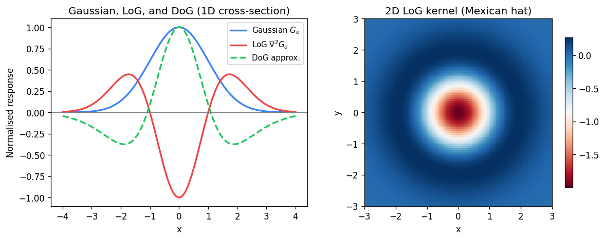
\[ \text{DoG} \approx G_\epsilon - G_\sigma \]where \( G_\epsilon \) is a very narrow Gaussian approximating a delta function (corresponding to the \( I \) term) and \( G_\sigma \) is the broader smoothing Gaussian. The DoG kernel has a characteristic appearance: a bright positive center surrounded by a negative annular ring, sometimes described as a “Mexican hat” shape.
Laplacian of Gaussian (LoG)
The Laplacian of Gaussian (LoG) is a closely related operator defined as the Laplacian (sum of second-order partial derivatives) applied to a Gaussian-smoothed image:
\[ \text{LoG} = \nabla^2 G_\sigma = \frac{\partial^2 G_\sigma}{\partial x^2} + \frac{\partial^2 G_\sigma}{\partial y^2} \]Like the DoG, it has a bright center and negative surround (or vice versa depending on sign convention). The LoG and DoG are closely approximated by each other for appropriate choices of the two Gaussian widths, and both are used as blob detectors: they respond strongly at circular intensity blobs — regions that are brighter (or darker) than their surroundings on a scale determined by \( \sigma \). The extrema (maxima and minima) of the DoG or LoG response over the image indicate locations and scales of blob-like features.
An important observation is that these kernels look visually like the patterns they are designed to detect. The derivative-of-Gaussian kernel in the x-direction resembles a vertical stripe pattern, and indeed it produces strong responses at vertical edges. A DoG kernel resembles a circular blob, and it produces strong responses at blob-like features. This visual correspondence between a kernel and the features it detects is the foundation of template matching and normalized cross-correlation.
Normalized Cross-Correlation (NCC) for Template Matching
Cross-Correlation as Similarity
Any linear filter applied to a location in an image can be interpreted as computing the dot product between the kernel \( h \) (unrolled into a vector) and the image patch \( f_t \) at that location (also unrolled). This is precisely cross-correlation. The numerical output of plain cross-correlation depends on the absolute magnitudes of the kernel and patch values, making it sensitive to illumination changes. To obtain a similarity measure that is invariant to scaling, one divides by the norms of both vectors, computing the cosine of the angle between them:
\[ \text{NCC}[t] = \frac{h \cdot f_t}{\|h\|\, \|f_t\|} = \cos\theta \]This is the Normalized Cross-Correlation (NCC). Its values lie in \( [-1, +1] \): a value of \( +1 \) means the patch is a positive scalar multiple of the template (perfect similarity); \( -1 \) means it is a negative multiple (opposite appearance); \( 0 \) means the two are orthogonal (uncorrelated).
Mean Subtraction and the Correlation Coefficient
A practical refinement is to subtract the mean value from both the template and the patch before computing the dot product and norms:
\[ \text{NCC}[t] = \frac{(h - \bar{h}) \cdot (f_t - \bar{f}_t)}{\|h - \bar{h}\|\, \|f_t - \bar{f}_t\|} \]This is equivalent to the standard Pearson correlation coefficient between the two samples. Equivalently, it can be written in terms of covariance and standard deviations:
\[ \text{NCC}[t] = \frac{\text{cov}(h, f_t)}{\sigma_h\, \sigma_{f_t}} \]Mean subtraction has two important effects. First, it removes additive intensity biases, making the similarity measure invariant to uniform brightness offsets between the template and the image patch. Second, because image intensities are always positive, the raw vectors always lie in the positive quadrant of their vector space; subtracting the mean centers them so they can point in any direction, allowing the full range from \( -1 \) to \( +1 \) to be achieved in practice.
Template matching via NCC produces a response image where local maxima indicate positions where the template best matches the underlying image content. Non-maximum suppression can be applied to these response maps to extract a sparse set of detected feature locations. As a simple but illustrative application, one can detect facial landmarks — left eye, right eye, mouth corners — by sliding templates for each part across a face image and finding local NCC maxima, then using spatial consistency constraints among the detected parts to prune false positives.
Feature Detectors
Discriminant Feature Points
For many applications — image alignment, 3D reconstruction, panoramic stitching, object recognition — one needs to establish reliable correspondences between points in two images of the same scene taken from different viewpoints. This requires discriminant feature points: locations whose appearance is sufficiently distinctive that they can be reliably identified in both images and matched correctly. Edges alone fail this criterion: along a straight edge, every local patch looks nearly identical to every other patch, and there is no way to determine which point on one edge corresponds to which point on another.
Harris Corner Detector
Corners are far more discriminant. At a corner, intensity gradients vary significantly in direction across the local neighborhood — there are multiple distinct edge directions — making the appearance unique. The Harris corner detector formalizes this intuition mathematically.
The key idea is to measure how much the image patch changes when the analysis window is shifted in each direction. Define the change function for a window \( w \) shifted by \( \mathbf{ds} = (u, v)^T \):
\[ E_w(u, v) = \sum_{x, y} w(x, y)\, [I(x + u, y + v) - I(x, y)]^2 \]where \( w(x, y) \) is 1 inside the window and 0 outside (or a Gaussian weighting). Using a first-order Taylor expansion of \( I(x+u, y+v) \) around \( (x, y) \):
\[ I(x + u, y + v) - I(x, y) \approx I_x\, u + I_y\, v = \nabla I \cdot \mathbf{ds} \]where \( I_x = \partial I/\partial x \) and \( I_y = \partial I/\partial y \) are the image gradients. Substituting and simplifying:
\[ E_w(u, v) \approx \mathbf{ds}^T\, M_w\, \mathbf{ds} \]where \( M_w \) is the \( 2 \times 2 \) structure tensor (also called the Harris matrix or autocorrelation matrix):
\[ M_w = \sum_{x, y} w(x, y)\, \nabla I\, \nabla I^T = \sum_{x, y} w(x, y) \begin{bmatrix} I_x^2 & I_x I_y \\ I_x I_y & I_y^2 \end{bmatrix} \]This matrix is computed by summing the outer products of the gradient vector at every pixel within the window, and it is always positive semi-definite.
Eigenvalue Analysis
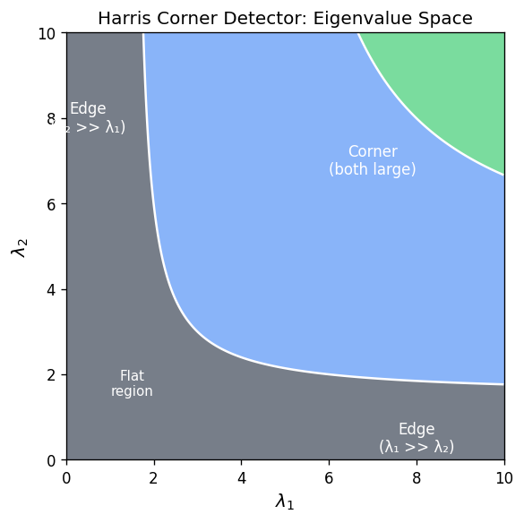
The function \( E_w(u, v) = \mathbf{ds}^T M_w \mathbf{ds} \) is a quadratic form whose isolines (level sets) are ellipses in the \( (u, v) \) plane. The shape of these ellipses is determined by the two eigenvalues \( \lambda_1, \lambda_2 \) of \( M_w \), and the orientation of the principal axes is given by the corresponding eigenvectors.
- If both \( \lambda_1 \) and \( \lambda_2 \) are small, the error \( E_w \) remains nearly zero even for large shifts in any direction: the window lies in a flat region with no texture.
- If one eigenvalue is large and the other small (say \( \lambda_2 \gg \lambda_1 \), the error grows rapidly in one direction but slowly in the other: the window lies on an edge, where sliding along the edge produces no change but crossing it produces a large change.
- If both \( \lambda_1 \) and \( \lambda_2 \) are large, the error grows rapidly in all directions: the window is at a corner, meaning the appearance changes significantly no matter which direction one moves.
The semi-axes of the ellipse are proportional to \( 1/\sqrt{\lambda_i} \), so large eigenvalues correspond to small ellipses (rapid change), and small eigenvalues correspond to large ellipses (slow change).
Harris Corner Response Measure
To avoid explicitly computing eigenvalues (which is computationally more expensive than computing determinant and trace), a common corner response function is:
\[ R = \frac{\det M_w}{\operatorname{trace} M_w} = \frac{\lambda_1 \lambda_2}{\lambda_1 + \lambda_2} \]Since \( \det M_w = \lambda_1 \lambda_2 \) and \( \operatorname{trace} M_w = \lambda_1 + \lambda_2 \), this ratio is large only when both eigenvalues are large, corresponding to a corner. Thresholding \( R > T \) and then applying non-maximum suppression yields a sparse set of corner locations.
Properties of the Harris detector:
- Rotation invariance: The eigenvalues of \( M_w \) (and hence \( R \) are invariant to image rotation, because rotating the image merely rotates the ellipse without changing its shape. Corner locations detected are therefore the same regardless of image orientation.
- Partial invariance to affine intensity changes: Adding a constant bias to all intensities does not affect gradients, so \( R \) is invariant to bias. Multiplying all intensities by a gain \( a \) scales the gradients and hence scales \( R \), but does not change the locations of local maxima — only potentially moving some above or below the detection threshold.
- Non-invariance to image scale: At a fine scale, a curved boundary segment may appear to be an edge; at a coarser scale (after zooming out), the same segment exhibits the abrupt directional change characteristic of a corner. The window size needed to detect the corner correctly depends on the scale at which it occurs, and Harris corners with a fixed window size will miss corners at other scales.
Scale-Invariant Feature Detection and the Gaussian Pyramid
The Scale Problem
The Harris detector’s non-invariance to scale is a fundamental limitation for matching across images taken at different distances or zoom levels. The solution is to search for features not just at a fixed scale but across a range of scales, selecting for each candidate location the scale at which the feature response is locally maximal. This adds scale as a third coordinate alongside \( x \) and \( y \).
Gaussian Pyramid
Rather than enlarging the filter kernel (which is computationally expensive), the standard approach is to downsample the image while keeping the kernel fixed. The Gaussian pyramid is a multi-resolution representation constructed by repeated blur-and-downsample operations:
- Start with the original image at full resolution.
- Blur with a Gaussian and downsample by a factor of 2, producing a half-resolution image.
- Repeat, producing progressively coarser levels.
Each level of the pyramid corresponds to a different scale. Because each successive image has half the resolution, the total storage cost of the pyramid is only about \( 4/3 \) times that of the original image (geometric series). Convolving each pyramid level with the same DoG kernel is equivalent to convolving the original image with a DoG kernel scaled up by the pyramid factor — a much more efficient approach.
The Gaussian pyramid bears a resemblance to the encoder portion of segmentation convolutional neural networks: both apply repeated convolution and downsampling to process an image at multiple resolutions. This connection is not coincidental and will resurface when CNNs are covered later in the course.
Scale-Space Feature Detection with DoG
To find blob-like features at their natural scale, convolve the DoG kernel with each level of the Gaussian pyramid, producing a 3D volume indexed by position \( (x, y) \) and scale \( s \). Local maxima in this 3D volume — points that are larger than all their neighbors in position and in scale — are reported as detected features. Each feature is characterized by its location \( (x, y) \) and its scale \( s \), often visualized as a circle whose center is the feature location and whose radius is proportional to the feature scale.
Feature Descriptors
Detection vs. Description
Detecting a feature point gives its location and scale. To match feature points across images, one also needs a descriptor: a compact representation of the local image appearance that is stable across viewpoint and illumination changes, and distinctive enough to avoid incorrect matches. A good descriptor must be both invariant (stable to common transformations) and discriminant (different for different features).
The hierarchy of discriminancy, from least to most:
- Color (RGB): Very few distinct colors; almost any two nearby patches can be confused. Non-discriminant.
- Edges (gradient magnitude extrema): More distinctive but still insufficient — patches at different positions along the same edge look identical.
- Corners: Highly distinctive in location; the basis for MOPS and SIFT descriptors.
Rotation Invariance via Dominant Gradient
A key invariance requirement is robustness to rotation: if the same scene is photographed from a rotated viewpoint, descriptors for the same physical point should be similar. The standard trick is to define a canonical orientation for each feature based on the dominant gradient direction in its neighborhood.
The dominant gradient is computed at a coarser scale (by blurring the image heavily) to get a stable, noise-robust estimate of the overall intensity gradient direction. This direction is then used to rotate the analysis patch into a consistent canonical frame. If the same feature is observed from a rotated camera, both detections will estimate the same (rotated) dominant gradient and both will canonically orient their patches accordingly — so the resulting patches, though extracted from differently oriented images, will be aligned and comparable.
Multi-Scale Oriented Patches (MOPS)
MOPS (Multi-Scale Oriented Patches) is a complete feature description system built on Harris corners. For each detected Harris corner at scale \( s \) and location \( (x, y) \):
- Scale and location come from the Harris detector applied at each pyramid level.
- Orientation is determined by the dominant blurred-gradient direction in the neighborhood, making the descriptor rotation-invariant.
- Descriptor vector: A square image patch of size proportional to \( 5s \times 5s \) pixels is sampled around the feature center, aligned with the canonical orientation. This patch is resampled to a standard \( 8 \times 8 \) grid using grayscale intensities.
- Normalization: The 64 grayscale values are normalized by subtracting the mean and dividing by the standard deviation within the patch: \( I' = (I - \mu)/\sigma \). This achieves bias/gain invariance: if the same patch is observed under different uniform lighting (additive bias \( I \to I + b \) or multiplicative gain (\( I \to aI \), the normalized descriptor is unchanged.
Matching is performed by comparing descriptors at the same scale: a feature at scale \( s \) in one image is matched against features at scale \( s \) in another, using Euclidean distance between descriptor vectors as the matching score.
SIFT (Scale-Invariant Feature Transform)
SIFT (Scale-Invariant Feature Transform), introduced by David Lowe, is arguably the most widely cited paper in the history of computer vision and remains a benchmark for hand-crafted feature descriptors.
Detection: SIFT uses DoG extrema in the Gaussian pyramid — the same mechanism described above for scale-space feature detection — to find interest points at their natural scale. Like MOPS, each detected point has a location \( (x, y) \) and a scale \( s \).
Orientation assignment: Like MOPS, SIFT establishes a dominant orientation from the distribution of gradient orientations in the neighborhood, computed from the Gaussian-smoothed image at the detection scale. Typically, a histogram of gradient orientations is built from the neighborhood, with each gradient contribution weighted by its magnitude and by a Gaussian distance weight. The peak of this histogram defines the canonical orientation. Multiple peaks above 80% of the maximum can produce multiple descriptors for the same keypoint, increasing robustness.
Descriptor construction: The distinctive element of SIFT is its descriptor. Rather than using raw intensity values like MOPS, SIFT uses gradient orientation histograms. The neighborhood around the feature is divided into a \( 4 \times 4 \) grid of sub-regions. Within each sub-region, an 8-bin histogram of gradient orientations is computed, with gradient magnitudes providing the voting weights. Concatenating these \( 4 \times 4 \times 8 = 128 \) values produces the 128-dimensional SIFT descriptor. This representation is much more robust to small geometric distortions, local illumination variations, and minor viewpoint changes than raw intensity patches. The descriptor is subsequently L2-normalized and then clamped at 0.2 to reduce sensitivity to non-linear illumination effects, and renormalized.
The use of gradient orientation histograms gives SIFT invariance to intensity shifts and gains (since gradients are invariant to additive offsets), and the histogramming provides robustness to small spatial displacements. The result is a descriptor that is highly discriminant and stable across a wide range of photometric and geometric changes, which explains why SIFT was for many years the de-facto standard for feature-based image matching in tasks such as panoramic stitching, 3D reconstruction, and object recognition.
Summary
This lecture has covered the full pipeline from raw pixel values to sophisticated, matchable feature descriptors:
Point processing (gamma correction, histogram equalization, window-center adjustment) modifies pixel intensities independently to improve visual quality or adapt dynamic range.
Linear filtering via convolution or cross-correlation extracts neighborhood-based features. The mean filter smooths by uniform averaging; the Gaussian filter smooths with rotational invariance and explicit scale control through \( \sigma \). The derivative-of-Gaussian filter simultaneously smooths and differentiates, producing gradient estimates robust to noise. Sobel and Prewitt operators are practical approximations that incorporate local smoothing.
Non-linear filtering via the median filter handles impulsive (salt-and-pepper) noise more robustly than any linear filter, at the cost of no longer being expressible as a convolution.
Image gradients provide the fundamental low-level features for edge detection. The gradient vector at each pixel points in the direction of steepest intensity ascent; its magnitude quantifies edge strength. Non-maximum suppression thins thick edge bands to one-pixel-wide ridges. The Laplacian of Gaussian (LoG) and Difference of Gaussians (DoG) extend differentiation to second-order operators that detect blob-like structures.
Normalized Cross-Correlation unifies filtering with template matching, providing a statistically grounded similarity measure — the Pearson correlation coefficient — between a template and image patches at all locations.
Feature detectors identify discriminant locations for reliable cross-image matching. The Harris corner detector uses the eigenvalues of the structure tensor \( M_w \) to classify image patches as flat, edge, or corner. Its corner response function \( R = \det M_w / \operatorname{trace} M_w \) is rotation-invariant but scale-dependent.
Scale-invariant detection via the Gaussian pyramid finds features at their natural scale as local maxima in a \( (x, y, s) \) scale-space volume. MOPS adds orientation normalization and uses normalized intensity patches as descriptors. SIFT further replaces raw intensities with gradient orientation histograms, producing a robust 128-dimensional descriptor that was the state of the art in hand-crafted feature matching for over a decade.
Image Warping
Parametric Transformations
Image warping — also called a domain transformation — is distinct from the point processing (range transformations) studied in the previous lecture. Where point processing changes the intensity values of pixels while leaving their positions fixed (producing, for example, a brighter image whose geometric structure is unchanged), image warping moves pixels to new locations while preserving their intensity values. Formally, if \( f \) is the source image and \( T \) is a coordinate transform, then point processing produces \( g(\mathbf{x}) = T(f(\mathbf{x})) \), whereas image warping produces \( g(\mathbf{x}) = f(T(\mathbf{x})) \). The domain of the image is changed; the range (the set of intensity values) is merely rearranged.
This lecture focuses exclusively on parametric (global) warps — transformations that are described by a small, fixed number of parameters and that apply the same coordinate-changing rule to every pixel in the image. The word “global” emphasizes this uniformity: a single mathematical formula, controlled by just a handful of numbers, dictates the fate of every point. The simplest parametric warps use only four parameters (a 2×2 matrix), and even the most general class covered here — the projective transformation or homography — requires only eight independent parameters. This economy of description stands in sharp contrast to an arbitrary pixel permutation, which would require storing one pair of coordinates for every pixel in the image.
The full family of parametric warps studied here forms a nested hierarchy: linear transformations (scale, rotation, shear, reflection) are embedded within affine transformations (which add translation), which are in turn embedded within projective transformations. Each step up the hierarchy adds degrees of freedom and relaxes geometric invariants. The practical motivation for understanding this hierarchy is that the simplest transformation sufficient for a given task should always be preferred — simpler models are easier to estimate, are less prone to overfitting, and have faster inverses.
Linear Transformations: Scaling, Rotation, Shear, and Reflection
A 2D linear transformation maps every point \( \mathbf{p} = (x, y)^T \) to a new point \( \mathbf{p}' = (x', y')^T \) by matrix multiplication with a 2×2 matrix \( M \):
\[ \begin{pmatrix} x' \\ y' \end{pmatrix} = M \begin{pmatrix} x \\ y \end{pmatrix} = \begin{pmatrix} a & b \\ c & d \end{pmatrix} \begin{pmatrix} x \\ y \end{pmatrix}. \]The four entries of \( M \) constitute the four parameters of the transformation. A key property shared by all linear transformations is that the origin always maps to the origin: setting \( (x, y) = (0, 0) \) always yields \( (x', y') = (0, 0) \).
Scaling is the simplest non-trivial example. A uniform scaling by factor \( s \) multiplies both coordinates equally; non-uniform scaling uses a diagonal matrix with independent scale factors \( s_x \) and \( s_y \) along each axis:
\[ S = \begin{pmatrix} s_x & 0 \\ 0 & s_y \end{pmatrix}. \]The inverse is obtained by reciprocating the diagonal entries. When \( s_x \neq s_y \) the transformation changes the aspect ratio of the image, stretching it along one axis relative to the other.
2D rotation about the coordinate origin by angle \( \theta \) (counterclockwise) is derived by expressing a point in polar form. If a point has polar coordinates \( (r, \phi) \), so that \( x = r\cos\phi \) and \( y = r\sin\phi \), then after rotation by \( \theta \) it becomes \( x' = r\cos(\phi+\theta) \) and \( y' = r\sin(\phi+\theta) \). Expanding with the angle-addition identities and substituting back:
\[ x' = x\cos\theta - y\sin\theta, \qquad y' = x\sin\theta + y\cos\theta. \]In matrix form this is the rotation matrix:
\[ R(\theta) = \begin{pmatrix} \cos\theta & -\sin\theta \\ \sin\theta & \cos\theta \end{pmatrix}. \]Although \( \sin \) and \( \cos \) are nonlinear functions of the parameter \( \theta \), the mapping itself is still linear in \( (x, y) \) — each output coordinate is a linear combination of the input coordinates. Rotation matrices have only one genuine degree of freedom (the angle \( \theta \), even though the matrix has four nonzero entries. A crucial property is that the inverse of a rotation matrix equals its transpose: \( R^{-1} = R^T \). This holds because rotating by \( -\theta \) reverses the rotation, and substituting \( -\theta \) into the formula for \( R \) yields exactly the transpose.
Shear is a transformation that slides points parallel to one axis by an amount proportional to their coordinate along the other axis. A horizontal shear is written:
\[ \begin{pmatrix} x' \\ y' \end{pmatrix} = \begin{pmatrix} 1 & sh_x \\ 0 & 1 \end{pmatrix} \begin{pmatrix} x \\ y \end{pmatrix}, \]so that \( x' = x + sh_x \cdot y \) while \( y' = y \) is unchanged. Points on the same horizontal scan line (same \( y \) all shift by the same amount, but points at different heights shift differently. This is not a rotation: although lines through the origin map to lines at a different angle, the individual points translate horizontally rather than rotating around the origin.
Reflection is represented by diagonal matrices with negative entries. Mirroring about the \( y \)-axis negates only the \( x \)-coordinate:
\[ \begin{pmatrix} -1 & 0 \\ 0 & 1 \end{pmatrix}, \]while point reflection through the origin negates both coordinates with \( \text{diag}(-1, -1) \).
A fundamental result characterizes the complete geometric scope of 2×2 linear transformations: any linear transformation is some combination of scaling, rotation, shear, and reflection — and conversely, any such combination is linear. This can be made precise using the singular value decomposition (SVD): every 2×2 matrix \( A \) factors as
\[ A = R(\theta) \begin{pmatrix} \lambda_1 & 0 \\ 0 & \lambda_2 \end{pmatrix} R(-\phi), \]where the two rotation matrices define a pair of orthogonal coordinate axes, and the diagonal matrix performs a (possibly anisotropic) scaling along those axes. The scalars \( \lambda_1, \lambda_2 \) can be negative, which corresponds to a reflection. The overall area scaling factor is \( |\det A| = |\lambda_1 \lambda_2| \), and this factor is the same everywhere in the plane — ratios of areas are preserved under any linear transformation.
Key properties shared by all 2D linear transformations are: the origin maps to the origin; lines map to lines; parallel lines remain parallel; ratios of lengths along parallel lines are preserved; ratios of areas are preserved; and the set of linear transformations is closed under composition (the product of two 2×2 matrices is another 2×2 matrix).
What linear transformations cannot do: translation. The transformation \( x' = x + t_x, \; y' = y + t_y \) shifts every point by the fixed vector \( (t_x, t_y) \). It is not a linear transformation because \( T(0, 0) = (t_x, t_y) \neq (0, 0) \), violating the requirement that the origin maps to the origin. No 2×2 matrix can represent translation. This limitation motivates the introduction of homogeneous coordinates.
Linear Transformations as Space Deformation and Change of Basis
It is worth noting two complementary interpretations of the equation \( \mathbf{q} = M\mathbf{p} \). In the active (space deformation) interpretation, the matrix moves a point \( \mathbf{p} \) to a new location \( \mathbf{q} \) within a fixed coordinate system. In the passive (change of basis) interpretation, the columns of \( M \) are treated as new basis vectors \( \mathbf{u} \) and \( \mathbf{v} \), and the equation expresses that the coordinates \( (4, 3) \) (for example) in the new basis \( \{\mathbf{u}, \mathbf{v}\} \) correspond to the point \( \mathbf{q} \) expressed in the original basis \( \{\mathbf{i}, \mathbf{j}\} \). The inverse matrix \( M^{-1} \) then converts back — its columns play the role of \( \mathbf{i} \) and \( \mathbf{j} \) expressed in the \( \{\mathbf{u}, \mathbf{v}\} \) system. When both bases are orthonormal, the matrix \( M \) reduces to a rotation (or rotoreflection).
Homogeneous Coordinates
To include translation within the framework of matrix multiplication, we adopt homogeneous coordinates. A 2D point \( (x, y) \) is represented by a 3-vector \( (x, y, 1)^T \), or more generally by any scalar multiple \( (wx, wy, w)^T \) for \( w \neq 0 \). The rule for converting back to Cartesian coordinates is to divide the first two components by the third: the homogeneous triple \( (X, Y, W) \) represents the 2D point \( (X/W, \; Y/W) \). The triple \( (0, 0, 0) \) is forbidden since it yields \( 0/0 \).
This representation is deliberately redundant: infinitely many triples represent the same 2D point, since scaling all three components by any nonzero constant \( \lambda \) leaves the ratio unchanged. For instance, \( (2, 1, 1) \), \( (4, 2, 2) \), and \( (6, 3, 3) \) all represent the Cartesian point \( (2, 1) \).
With this representation, translation becomes a linear operation. Setting \( w = 1 \) and multiplying by the 3×3 translation matrix:
\[ \begin{pmatrix} 1 & 0 & t_x \\ 0 & 1 & t_y \\ 0 & 0 & 1 \end{pmatrix} \begin{pmatrix} x \\ y \\ 1 \end{pmatrix} = \begin{pmatrix} x + t_x \\ y + t_y \\ 1 \end{pmatrix}, \]which corresponds to the translated Cartesian point \( (x + t_x,\; y + t_y) \).
A second major advantage of homogeneous coordinates is that they give a finite representation to points at infinity. As the third coordinate \( w \to 0 \) with \( (x, y) \) held fixed, the Cartesian point \( (x/w, y/w) \) recedes to infinity along the ray in direction \( (x, y) \). The homogeneous triple \( (x, y, 0) \) — perfectly representable with ordinary floating-point numbers — encodes this point at infinity. This is the 2D analogue of the way \( \pm\infty \) extend the real line; here we get a whole circle’s worth of “directions at infinity” added to the Euclidean plane. The resulting space is the projective plane \( \mathbb{P}^2 \).
Affine Transformations
Once we work in homogeneous coordinates, all the linear transformations from before can be embedded in 3×3 matrices by placing the 2×2 part in the upper-left and filling the last row with \( (0, 0, 1) \). Adding nonzero entries \( t_x \) and \( t_y \) in the last column of the top two rows yields the general affine transformation:
\[ \begin{pmatrix} x' \\ y' \\ 1 \end{pmatrix} = \begin{pmatrix} a & b & c \\ d & e & f \\ 0 & 0 & 1 \end{pmatrix} \begin{pmatrix} x \\ y \\ 1 \end{pmatrix}. \]The bottom row is fixed as \( (0, 0, 1) \), so only the six entries \( a, b, c, d, e, f \) in the top two rows are free parameters — affine transformations have 6 degrees of freedom. This bottom-row constraint guarantees that the third coordinate of the output is always 1, so no division is needed to recover Cartesian coordinates; the transformation is automatically “non-projective.”
Affine transformations are exactly the combinations of linear transformations (scale, rotation, shear, reflection) with arbitrary translations. Any composition of affine transformations is again affine — the product of two 3×3 matrices whose bottom rows are \( (0, 0, 1) \) is again a 3×3 matrix with bottom row \( (0, 0, 1) \).
The geometric properties of affine transformations extend those of linear transformations by relaxing the constraint that the origin is fixed. Specifically: the origin does not necessarily map to the origin (because of the translation component); lines still map to lines; parallel lines remain parallel; ratios of lengths along parallel lines are preserved; ratios of areas are preserved; and the set is closed under composition and inversion.
These invariants — parallelism in particular — are central to understanding what affine transformations can and cannot do. A pair of parallel lines will always remain parallel after any affine warp; if your application requires parallel lines to converge (as they appear to do in a perspective photograph of a road), you need a strictly projective transformation.
Projective Transformations and Homographies
Projective transformations, also called homographies, are the most general linear transformations in homogeneous coordinate space. They are represented by general invertible 3×3 matrices with no constraints on the last row:
\[ \begin{pmatrix} x' \\ y' \\ w' \end{pmatrix} = \begin{pmatrix} a & b & c \\ d & e & f \\ g & h & i \end{pmatrix} \begin{pmatrix} x \\ y \\ 1 \end{pmatrix}. \]The output is a homogeneous triple \( (x', y', w') \), and the resulting Cartesian point is \( (x'/w', \; y'/w') \). Because the last row is no longer fixed to \( (0, 0, 1) \), the denominator \( w' = gx + hy + i \) can vary with position, producing a nonlinear (rational) map on Cartesian coordinates.
Although there are 9 entries in the matrix, multiplying the entire matrix by any nonzero scalar produces exactly the same projective transformation (because the division by \( w' \) cancels the common factor). Therefore homographies have only 8 degrees of freedom. The 9 parameters are determined only up to a global scale.
The properties of projective transformations are a superset of affine properties in some respects, but weaker in others. The origin does not necessarily map to the origin. Lines still map to lines — this is a fundamental theorem: an invertible mapping of the projective plane onto itself that preserves straight lines must be a homography, and conversely every homography preserves straight lines. However, parallel lines do not necessarily remain parallel: under a projective warp, two lines that were parallel may meet at a finite point, or two non-parallel lines may both be sent to lines that meet at a point at infinity (i.e., become parallel). Distance, length, and area ratios are not preserved. Only the incidence structure — which points lie on which lines — is invariant.
A concrete example illustrates the parallel-line behavior. Under a homography \( H \), a finite intersection point of two lines can map to the homogeneous triple \( (x', y', 0) \) — a point at infinity — meaning the images of the two lines are now parallel. Conversely, applying the inverse \( H^{-1} \) can bring a point at infinity back to a finite location, making formerly parallel lines converge. This is precisely the projective phenomenon visible in perspective photographs, where parallel rails of a railway appear to meet at a vanishing point.
The nested hierarchy of 2D transformations, from most constrained to most general, can be summarized by the structure they preserve:
| Transformation | DOF | Preserved invariants |
|---|---|---|
| Translation | 2 | Everything except position |
| Euclidean (rigid) | 3 | Shape, size, angles |
| Similarity | 4 | Shape, angles (not size) |
| Affine | 6 | Parallelism, area ratios |
| Projective | 8 | Straight lines only |
Each class is closed under composition and inversion, forming a group. Each is a subgroup of the next.
Estimating Transformations from Correspondences
In practice, one often knows a set of point correspondences — pairs \( (\mathbf{p}_i, \mathbf{p}'_i) \) where point \( \mathbf{p}_i \) in the source image corresponds to point \( \mathbf{p}'_i \) in the target image — and wants to recover the parametric transformation that explains them. The goal is to find the matrix \( M \) such that \( \mathbf{p}'_i \approx M\mathbf{p}_i \) for all pairs. How many correspondences are needed depends on the number of degrees of freedom.
Translation (2 DOF): One correspondence pair provides two equations (one for \( \Delta x \) and one for \( \Delta y \), exactly matching the two unknowns. A single pair suffices.
Euclidean / rigid (3 DOF: translation + rotation): Two pairs are needed. The first pair constrains where one point goes; the second pair additionally constrains the rotation angle. Geometrically, once two pairs of matched points are known, the rigid-body invariants (lengths and angles are preserved) allow one to construct the match of any third point without additional clicks: draw a perpendicular from the arbitrary point to the line connecting the two reference points, measure the distances, and reproduce the same distances and angle in the target image.
Affine (6 DOF): Three correspondence pairs are required. Each pair supplies two linear equations in the six unknowns \( a, b, c, d, e, f \). Explicitly, the affine equation \( \mathbf{p}'_i = M\mathbf{p}_i \) in homogeneous coordinates gives:
\[ x'_i = ax_i + by_i + c, \qquad y'_i = dx_i + ey_i + f. \]Three pairs yield six equations and six unknowns — a determined linear system, provided the three source points are not collinear (if they were, the system would be rank-deficient). Geometrically, the affine invariants of parallelism and length ratios are sufficient to construct the image of any fourth point from three known matches.
The triangle-warping application is a direct consequence: given triangles \( ABC \) and \( A'B'C' \) in two images, one solves the 6×6 affine system using the three corner correspondences to obtain the unique affine transformation mapping one triangle to the other. All interior pixels can then be warped accordingly. In mesh-based deformation models, each triangle in the mesh gets its own affine transformation; the overall warp is piecewise-affine, with six parameters per triangle.
Projective (8 DOF): Four correspondence pairs are required, yielding eight equations — exactly matching the eight degrees of freedom. Each pair still contributes two independent equations (the derivation of this, which involves eliminating the homogeneous scale, is deferred to a later topic). The four points must be in general position (no three collinear in either image). Geometrically, once four point correspondences are known, the line-preservation invariant of homographies allows one to recursively construct matched points for arbitrary fifth, sixth, … points by intersecting images of known lines — a process that can be continued indefinitely.
In practice, when the number of available correspondences exceeds the minimum (e.g., many matched feature points from a descriptor-matching step), the system is overdetermined. The standard solution is linear least squares: stack all the constraint equations into a matrix equation \( A\mathbf{m} = \mathbf{b} \) (or, for the homogeneous case appropriate to homographies, \( A\mathbf{m} = \mathbf{0} \) and solve for the parameter vector \( \mathbf{m} \) that minimizes the total squared residual. For the affine case the system is directly linear and the least-squares solution is \( \mathbf{m} = (A^T A)^{-1} A^T \mathbf{b} \). For homographies the appropriate formulation and solution via SVD will be discussed in a later lecture.
Forward and Inverse Warping
Given a source image \( f \), a target image \( g \), and a known parametric transformation \( T \) such that every source point \( (x, y) \) maps to target point \( (x', y') = T(x, y) \), the computational task is to fill in the pixel values of the discrete raster image \( g \). The difficulty is that \( T \) maps integer pixel coordinates to real-valued coordinates, and images are only defined at integer positions.
Forward Warping
In forward warping, one iterates over every source pixel \( (x, y) \), applies \( T \) to find the target location \( (x', y') \), and copies the intensity of \( f(x, y) \) to that location in \( g \). The problem is that \( (x', y') \) is generically a non-integer coordinate, lying between pixel centers in the target grid. One solution is splatting: distribute the source pixel’s intensity among the neighboring target pixels, weighted by proximity. However, forward warping has two serious failure modes. First, multiple source pixels may map to overlapping neighborhoods of the same target pixel, requiring the contributions to be blended — this is manageable. Second, and more critically, some target pixels may receive contributions from no source pixel at all, because all nearby source pixels map to other regions of the target grid. These holes in the target image are difficult to fill without additional processing.
Inverse Warping
Inverse warping (backward warping) avoids holes by reversing the direction of traversal. One iterates over every target pixel \( (x', y') \) and uses the inverse transformation \( T^{-1} \) to find the corresponding source location \( (x, y) = T^{-1}(x', y') \). Because every target pixel is visited exactly once, there can be no holes. For all parametric transformations discussed in this lecture, computing \( T^{-1} \) is straightforward — it is simply the inverse matrix. The remaining difficulty is that \( (x, y) \) is again a real-valued location lying between source pixels, so some form of interpolation is required to estimate \( f \) at that location.
The standard options for interpolation are: nearest-neighbor (copy the value of the single closest source pixel — fast but produces blocky artifacts); bilinear interpolation (smooth weighted average of the four surrounding pixels — the most common choice); bicubic interpolation (uses a 4×4 neighborhood for smoother results); and Gaussian (a larger weighted average). The tradeoffs involve computational cost versus smoothness.
Comparison and Artifacts
Both forward and inverse warping suffer when the transformation causes large area distortions. If the Jacobian of \( T \) has a determinant far from 1 — meaning the transformation locally stretches or shrinks areas significantly — artifacts appear regardless of the warping direction. Forward warping of a region that gets strongly stretched produces holes (the stretched region in the target receives too few painted pixels). Inverse warping of a region that gets strongly compressed produces aliasing: the inverse map visits only a sparse subset of source pixels in a small region, missing the fine texture detail and producing Moiré-like patterns. Proper antialiasing in the shrinking case requires supersampling or appropriate prefiltering, which is beyond the scope of this lecture.
For practical implementation, the skimage.transform.warp function in Python implements inverse warping. A common student error is to pass the forward transform as the second argument instead of its inverse: the function’s inverse_map argument must be a function that maps output-image coordinates to input-image coordinates, i.e., it implements \( T^{-1} \).
Bilinear Interpolation
Bilinear interpolation is the standard method for estimating image intensity at a non-integer location \( (x, y) \) from the four surrounding integer pixels. It is grounded in the concept of linear interpolation extended to two dimensions.
Linear interpolation in 1D. Given intensity values \( f(P) \) and \( f(Q) \) at two adjacent pixels \( P \) and \( Q \), any point between them can be written as a convex combination \( \lambda P + (1-\lambda) Q \) for \( \lambda \in [0, 1] \). Assuming \( f \) is linear between \( P \) and \( Q \), its value at the intermediate point is:
\[ f(\lambda P + (1-\lambda) Q) = \lambda f(P) + (1-\lambda) f(Q). \]This is simply a weighted average: the weight \( \lambda \) is the fractional distance from \( Q \) to the query point, and \( 1-\lambda \) is the fractional distance from \( P \).
Bilinear interpolation in 2D. Suppose the query point \( (x, y) \) lies within the unit cell whose four corners are at integer pixel positions \( (i, j) \), \( (i+1, j) \), \( (i, j+1) \), and \( (i+1, j+1) \). Define the fractional offsets \( a = x - i \) and \( b = y - j \), both in \( [0, 1] \). Bilinear interpolation proceeds in two stages:
- Interpolate horizontally along the bottom row to a point directly below \( (x, y) \):
- Interpolate horizontally along the top row to a point directly above \( (x, y) \):
- Interpolate vertically between these two intermediate values:
Combining these three steps yields the bilinear formula as a weighted sum of all four surrounding pixel values:
\[ f(x,y) \approx (1-a)(1-b)\,f(i,j) + a(1-b)\,f(i+1,j) + (1-a)b\,f(i,j+1) + ab\,f(i+1,j+1). \]The four weights sum to one, confirming this is a proper weighted average.
There is an elegant geometric interpretation of these weights. If each pixel is thought of not as a point but as a unit square cell centered at its integer coordinate, then the weight assigned to each of the four neighboring cells equals the area of overlap between that cell and a unit square centered at the query point \( (x, y) \). For instance, the weight for pixel \( (i, j) \) is the overlap area \( (1-a)(1-b) \) — a rectangle of width \( 1-a \) and height \( 1-b \). This area-overlap interpretation makes it clear why bilinear interpolation is a natural and physically motivated scheme: the interpolated value is the intensity one would measure if the pixel cell were a uniformly colored patch and you sampled a unit-area window centered at the query location.
Bilinear interpolation guarantees continuity of the interpolated function across the image domain — the result varies smoothly as the query location moves — though the gradient has discontinuities at the grid lines. When greater smoothness is required, bicubic interpolation (which fits a piecewise cubic and matches derivatives at grid points) is preferred at the cost of consulting a larger 4×4 neighborhood and heavier computation.
Mosaics — Homographies and Blending
Motivation: Expanding the Field of View
A standard compact camera or smartphone has a field of view of roughly 50° × 35°. The human visual system, by contrast, perceives a field of roughly 200° × 135°, and a full spherical panorama extends to 360° × 180°. Closing this gap is the core motivation behind image mosaicing: the computational process of stitching several overlapping photographs taken from the same vantage point into one wide-angle composite image.
Mosaicing is one of the earliest real success stories of computer vision. The algorithms described in this lecture underpin the panorama modes found in virtually every modern smartphone camera. The critical geometric insight is that if the camera rotates around its fixed optical center without translating, every pair of images it produces is related by a homography — a projective transformation — and this relationship makes accurate registration and stitching possible without any explicit knowledge of the 3D scene.
The basic requirement for stitching is that consecutive images must overlap. Without overlap there are no common scene points to use as anchors for registration, and the stitched result will contain holes. In practice this means rotating the camera in small enough steps that adjacent frames share a visible strip of the scene.
The Panorama Pipeline
Building a panoramic mosaic is a multi-stage pipeline. At a high level the steps are:
- Capture a sequence of images by rotating the camera about its optical center.
- Detect distinctive feature points in each image.
- Match features across pairs of overlapping images to establish point correspondences.
- Estimate a homography from those correspondences, using RANSAC to reject mismatches.
- Warp each image onto a common projection surface (a plane, cylinder, or sphere).
- Blend the warped images to produce a seamless mosaic.
For a sequence of images the standard practice is to choose the image roughly in the center of the sequence as the common projection plane (PP). Choosing the center minimizes the maximum rotation angle any single image must undergo, which in turn minimizes projective distortion. The images are then reprojected one by one onto this common plane, typically processing consecutive pairs so that each step has large overlap and the accumulated warping error stays small.
An important geometric fact is that scene knowledge is not required to build a mosaic, as long as the camera center is stationary. The only geometric requirement is shared: all images must share a single center of projection. When that condition holds, every pair of image planes is related by a homography, regardless of the 3D scene content.
Review: The Pinhole Camera and Ray Correspondences
Recall from the pinhole camera model (Lecture 2) that every camera has an optical center (viewpoint) and an image plane separated from the center by the focal length \( f \). We conventionally place a virtual image plane in front of the optical center. A scene point \( X \) is imaged at pixel \( p \), the intersection of the ray from \( X \) through the optical center with the image plane.
When the camera rotates around its fixed optical center, two image planes \( \text{PP}_1 \) and \( \text{PP}_2 \) share the same set of rays. Any ray that intersects both planes defines a pair of corresponding pixels: the two pixels record the same scene point and therefore the same color. This collection of ray-based correspondences defines a warp — a function that maps every pixel in one image to a pixel in the other. The existence of this warp (and nothing else) is what makes mosaicing possible.
Why is translation-only registration insufficient? Two images taken from a rotating camera cannot be aligned by a pure translation, because the perspective distortion varies spatially. Rail tracks on a flat road are parallel in 3D but converge to a vanishing point in each image; any simple offset leaves them misaligned. A richer class of transforms is needed.
Homography: The Right Transformation Class
A homography (also called a projective transformation) is the unique 2D transformation that maps straight lines to straight lines and, among the standard classes (translation, Euclidean, affine, projective), is both necessary and sufficient to describe the central projection of one image plane onto another sharing the same optical center.
Proof that homographies are sufficient. Take an arbitrary line \( \ell \) in \( \text{PP}_2 \). The set of rays through all points of \( \ell \) and the optical center \( C \) forms a plane \( \Pi \). The intersection of \( \Pi \) with \( \text{PP}_1 \) is also a line (two planes intersect in a line). Therefore ray correspondences map lines to lines, which — by the characterization theorem for homographies — implies the mapping is a homography.
Proof that affine transformations are insufficient. Affine transforms must preserve parallelism. But parallel rail tracks on a flat ground plane converge to a vanishing point when projected onto an image plane. Parallelism is not preserved, so affine transforms cannot describe central projection in general.
Homographies have 8 degrees of freedom (DOF) — a 3 × 3 matrix \( H \) defined up to an overall scale factor, giving \( 9 - 1 = 8 \) free parameters. In homogeneous coordinates, the mapping is:
[ \begin{pmatrix} wx’ \ wy’ \ w \end{pmatrix}
\begin{pmatrix} a & b & c \ d & e & f \ g & h & i \end{pmatrix} \begin{pmatrix} x \ y \ 1 \end{pmatrix} ]
The point \( p = (x, y) \) maps to \( p' = (x', y') \), where the output is recovered by dividing by the scale factor \( w = gx + hy + i \):
\[ x' = \frac{ax + by + c}{gx + hy + i}, \qquad y' = \frac{dx + ey + f}{gx + hy + i} \]A crucial subtlety: when writing the matrix equation, the input \( p \) can be represented as \( (x, y, 1)^T \), but the output \( (wx', wy', w)^T \) does not generally have its third coordinate equal to 1. The scale \( w \) is an additional unknown that must be eliminated algebraically.
Computing the Homography
Given a correspondence \( (x, y) \to (x', y') \), expanding the homogeneous matrix equation and eliminating \( w \) by substituting \( w = gx + hy + i \) yields two linear equations in the nine unknowns \( \{a, b, c, d, e, f, g, h, i\} \):
\[ ax + by + c - gx \cdot x' - hy \cdot x' - i \cdot x' = 0 \]\[ dx + ey + f - gx \cdot y' - hy \cdot y' - i \cdot y' = 0 \]These equations are linear in the unknowns (the known coordinates \( x, y, x', y' \) act as coefficients). Each correspondence contributes exactly two such equations, so four point correspondences give eight equations for nine unknowns. The ninth equation comes from a normalization constraint. A common choice is to fix \( i = 1 \).
When is \( i = 1 \) safe? Setting \( i = 1 \) is equivalent to assuming \( i \neq 0 \); if \( i \neq 0 \), we can always rescale \( H \) (which leaves the transformation unchanged, since homographies are defined up to scale) so that \( i = 1 \). The edge case where \( i = 0 \) occurs exactly when the origin of the first image maps to a point at infinity in the second — a situation that arises when the rotation angle is very large. In practice this is rare, but the next topic introduces a completely robust normalization constraint (SVD-based) that avoids making this assumption.
This linear system is an instance of the Direct Linear Transform (DLT) method. When more than four correspondences are available — as is typical with automatic feature matching — the system is overdetermined and solved in the least-squares sense, again via SVD. Using more correspondences improves robustness against noise.
When Does Mosaicing Require Only Camera Rotation?
The assumption of a fixed optical center is important. If the camera both rotates and translates, ray correspondences between two image planes no longer define a consistent warp for a general 3D scene. Points at different depths project to different locations in each image, and no single homography can reconcile these depth-dependent shifts — this is the parallax problem.
There are two exceptions where mosaicing still works even with camera translation:
Planar scenes. If the scene lies on a single plane (e.g., photographing a large whiteboard at close range), then the projection from the scene plane to each camera image is a homography, and the composition of two such homographies is also a homography. Any two photos of the same flat surface are related by a homography regardless of where the cameras are. This is how large-scale aerial mosaics of flat terrain are made.
Far-away scenes. When the scene is very far from the camera relative to the camera baseline, the parallax becomes negligible and the homography approximation is again accurate.
Cylindrical Projection for Wide Panoramas
For panoramas approaching 360° horizontal extent, projecting everything onto a flat plane is impractical: images taken near 90° from the reference suffer extreme distortion, and images beyond 90° cannot be projected at all (they end up “behind” the reference plane). The standard solution is to project each image onto a common cylinder (or sphere) instead.
In cylindrical projection each image pixel is first “unwarped” from its flat perspective projection onto the surface of a cylinder of radius \( f \) (the focal length). For a pixel at position \( (x, y) \) in an image with principal point at the center, the corresponding cylindrical coordinates \( (\hat{x}, \hat{y}) \) are:
\[ \hat{x} = f \arctan\!\left(\frac{x}{f}\right), \qquad \hat{y} = \frac{f \cdot y}{\sqrt{x^2 + f^2}} \]After this warping, the cylindrical image of each frame is a strip on the cylinder’s surface. Crucially, when the camera rotates purely horizontally, the cylinder strips align by a simple horizontal translation — matching in cylindrical space reduces to finding the translation offset between adjacent strips. This makes registration straightforward and drift-free for a full 360° sweep.
The trade-off is that the warp to the cylinder is not a homography: straight lines in the original images become curves on the cylinder. This means the DLT-based homography estimation described above cannot be applied directly in cylindrical space; however, for nearly horizontal panoramas the cylindrical model gives excellent results with minimal distortion.
Feature Detection and Matching for Alignment
Rather than requiring a user to click corresponding points manually, practical mosaicing systems detect and match salient feature points automatically. A good feature detector must find points that are repeatable — a point detected in one image should be detected at the same scene location when viewed from a slightly different angle and lighting.
Harris corner detection identifies points where image gradients are large in two orthogonal directions — i.e., genuine corners rather than edges or flat regions. The Harris response is computed from the second-moment matrix of local image gradients:
\[ M = \sum_{(x,y) \in W} \begin{pmatrix} I_x^2 & I_x I_y \\ I_x I_y & I_y^2 \end{pmatrix} \]where the sum is over a local window \( W \). A point is declared a corner when both eigenvalues of \( M \) are large — equivalently, when the Harris response \( R = \det(M) - k\,(\text{tr}(M))^2 \) exceeds a threshold (with \( k \approx 0.04 \)–0.06).
Harris corners are repeatable under small rotations and moderate illumination changes, but they are not scale-invariant. For more robust matching across significant scale changes (e.g., photos taken at different zoom levels), SIFT (Scale-Invariant Feature Transform) detects keypoints at multiple scales and describes each one with a 128-dimensional gradient histogram that is invariant to rotation and approximately invariant to illumination.
Once features are detected in each image, feature matching compares the descriptor of each keypoint in one image to all descriptors in the other, typically finding the nearest neighbor in descriptor space. A ratio test (Lowe’s ratio test) rejects ambiguous matches: a match is accepted only if the closest descriptor distance is significantly smaller than the second-closest. The remaining candidate matches still include some outliers (wrong matches from repetitive textures or descriptor collisions), which is why RANSAC is necessary.
RANSAC for Robust Homography Estimation
RANSAC (Random Sample Consensus) is the standard algorithm for robustly fitting a parametric model when a substantial fraction of the data are outliers. Applied to homography estimation:
- Sample 4 feature correspondences at random (the minimum needed to determine a homography).
- Fit the homography \( H \) to those 4 pairs using DLT.
- Score every other correspondence: count it as an inlier if the reprojection error \( \|p' - Hp\| \) is below a threshold \( \epsilon \).
- Repeat for many iterations and keep the hypothesis with the most inliers.
- Refit \( H \) using all inliers of the best hypothesis, in a least-squares sense.
RANSAC tolerates a large fraction of outliers and produces a reliable homography estimate even when automatic feature matching has a 50% or higher mismatch rate. The number of iterations needed is determined by the inlier fraction and the sample size; for mosaicing, a few hundred iterations is typically sufficient.
Image Warping to a Common Plane
With the homography \( H \) from image 2’s plane to image 1’s plane in hand, every pixel \( q \) in the output mosaic can be filled by inverse warping: compute \( H^{-1} q \) to find the corresponding location in image 2, then interpolate image 2’s pixel values there (using bilinear interpolation to avoid aliasing). Regions of the output that lie outside the source image’s footprint are left black (or transparent).
For a mosaic of many images, a common reference plane is chosen (typically the central image) and homographies are composed: the transform from image \( k \) to the reference is the product of successive pairwise homographies along the chain.
Image Blending
After warping, the overlap region between two images must be composited. Naively copying one image on top of the other leaves a sharp seam; averaging the two at constant \( \alpha = 0.5 \) suppresses high-frequency structure and looks blurry. The solution is alpha blending with spatially varying weights that change smoothly across the overlap.
Feathering via Distance Transforms
A principled and automatic approach (Danielsson, 1980) weights each image’s contribution at any pixel according to that pixel’s distance to the image boundary. Formally, define a distance map \( w_i(p) \) for image \( i \) as the distance from pixel \( p \) to the nearest border of image \( i \)’s support region. By definition, \( w_i = 0 \) at the boundary and increases toward the interior.
The normalized alpha weight for image \( i \) at pixel \( p \) is then:
\[ \alpha_i(p) = \frac{w_i(p)}{\sum_j w_j(p)} \]By construction, \( \sum_i \alpha_i(p) = 1 \) everywhere. Where only one image covers a pixel, that image’s \( w \) is the only nonzero term and its alpha is 1. In the overlap zone, the weights interpolate smoothly. The blended mosaic pixel is then:
\[ I_\text{blend}(p) = \sum_i \alpha_i(p)\, I_i(p) \]For the assignment, the distance to the border of a rectangular image region has a closed-form expression (minimum of distances to the four edges), so no general distance-transform algorithm is required.
Practical Variants
Three variants of alpha for two overlapping images illustrate the trade-offs:
- Center seam (\( \alpha_1 = \mathbf{1}[w_1 > w_2] \): hard binary selection — one image wins at each pixel. Produces a sharp but positionally accurate seam; any exposure mismatch causes an abrupt jump.
- Blurred seam: the binary alpha map above is convolved with a Gaussian. The transition zone softens in proportion to the blur kernel width. Works well when images have closely matched exposures.
- Distance-weighted (feathering): \( \alpha_1 = w_1 / (w_1 + w_2) \). The smoothest option; effectively a linearly interpolated transition across the entire overlap region.
The feathering approach handles exposure variation gracefully because it smoothly averages out any gain or bias difference between images, but it can produce ghosting artifacts if moving objects appear in the overlap region (see below).
Ghost Artifacts
A ghost appears when the same region of a scene contains different content in two images being blended — most commonly because a person or vehicle moved between shots. The alpha-blended average of the two images then shows a semi-transparent “double” of the moving object. Ghosts violate the fundamental mosaicing assumption that the scene is static. Detection and handling of ghosts requires either selecting a single source image at each pixel (rather than blending), or using temporal median filtering when video streams are available.
Direct vs. Feature-Based Alignment
There are two broad strategies for estimating the alignment between images:
Feature-based alignment (the approach described throughout this lecture) works in two stages: extract sparse salient keypoints, match their descriptors across images, then fit a geometric model (homography) to the matches. It is robust, fast, and tolerates large baselines and illumination changes. The decoupling of detection, matching, and estimation makes it straightforward to apply RANSAC.
Direct (pixel-based) alignment works directly on image intensities, minimizing a measure of photometric difference — such as sum of squared differences (SSD) or normalized cross-correlation — over all pixels jointly, typically via iterative gradient descent. Direct methods are more accurate when the initialization is close (they can refine to sub-pixel precision) but are sensitive to large illumination changes and require a good initial estimate. They are computationally heavier for large displacements.
In panorama construction, feature-based alignment is the standard choice for the initial estimation of homographies, while direct refinement can optionally be applied afterward to fine-tune registration.
Extensions: 360° Panoramas and Video Mosaics
For full 360° panoramas, the flat-plane model is replaced with cylindrical or spherical projection as described above. In cylindrical space, adjacent image strips align by horizontal translation alone, making large-scale mosaicing efficient and avoiding the extreme distortion that a flat projection would introduce at large angles. The warp from each flat image to the cylinder is nonlinear (it curves straight lines), but it is computed analytically from the known focal length and is applied once as a preprocessing step.
Video mosaics extend the idea temporally: two or more stationary video cameras capture the same scene, their spatial relationship is described by a homography (or a richer model), and the streams are merged into a wide-angle video feed. The main additional challenge is frame synchronization. Examples include multi-camera coverage of a football field, where cameras positioned along opposite sidelines are stitched into a single panoramic view.
Geometric Model Fitting and RANSAC
Feature Matching Recap
Before fitting any geometric model, one must first detect and match features across images. This lecture builds directly on the feature detection methods covered in earlier topics, so it is worth briefly revisiting the landscape of detectors and descriptors before turning to the central problem of fitting.
Harris corner detection identifies points in an image where intensity changes significantly in two orthogonal directions — locations that resist sliding along any direction. The method computes a second-moment matrix from image gradients and finds pixels where both eigenvalues of that matrix are large. In practice, the corner_harris function from skimage.feature computes a cornerness response map, and corner_peaks extracts local maxima above a threshold.
Difference-of-Gaussian (DoG) blob detection, which underlies the celebrated SIFT (Scale-Invariant Feature Transform) descriptor, finds features as extrema across a scale-space pyramid of Gaussian-blurred images. Blobs detected this way are simultaneously localised in position and scale, making them far more repeatable under viewpoint and zoom changes than simple corner detectors. The blob_dog function provides a convenient implementation.
Once features are detected, each is described by a compact numerical vector — its descriptor — that should be invariant to nuisance factors such as illumination gain and bias, in-plane rotation, and modest perspective distortion. The MOPS descriptor samples an 8×8 oriented patch at five times the detection scale and normalises for gain and bias: \( I' = (I - \mu)/\sigma \). SIFT instead histograms gradient orientations within subregions of the patch, achieving both invariance to illumination and distinctiveness. Other popular descriptors include SURF, HOG, and the binary descriptor BRIEF.
Feature matching requires deciding, for each feature detected in one image, which feature in another image it most likely corresponds to. An exhaustive optimal approach — bipartite matching or quadratic assignment — is too expensive for practical use. The standard approach instead computes the Sum of Squared Differences (SSD) between descriptor vectors and, for each feature in the first image, finds the nearest neighbour in the second image. A match is accepted if
\[ \text{SSD}(\text{patch}_1, \text{patch}_2) < T \]for some threshold \( T \). The fundamental difficulty is that no fixed threshold cleanly separates true from false matches: the SSD distributions for correct and incorrect matches overlap substantially.
A much more reliable strategy was introduced by David Lowe in 1999 and is now nearly universally adopted. Rather than thresholding the absolute SSD of the best match, one computes the ratio of the SSD of the closest match (SSD1) to the SSD of the second-closest match (SSD2):
\[ \frac{\text{SSD}_1}{\text{SSD}_2} < T \]This Lowe ratio test accepts a match only when the best match is substantially better than all alternatives. A genuine correspondence tends to have a uniquely small SSD, so the ratio is small; a spurious match occurs in a crowded descriptor space where the ratio approaches one. In skimage, the match_descriptors function with cross_check=True also enforces mutual consistency: a pair \( (p, p') \) is retained only if \( p \) is the best match for \( p' \) and \( p' \) is the best match for \( p \). Even with these safeguards, a non-trivial fraction of matches will be incorrect — a fact that motivates everything that follows.
Model Fitting and Least Squares
The central geometric task of this lecture is homography estimation: given a set of point correspondences \( \{(p_i, p'_i)\} \) between two images, find the \( 3\times 3 \) projective transformation \( H \) such that \( p'_i \approx H p_i \) in homogeneous coordinates. A panorama assembled from images taken by a rotating camera can always be related by a homography, because the camera rotation maps every 3D ray to another 3D ray, and two images of the same set of rays are projectively equivalent. The question is how to estimate \( H \) reliably and automatically.
Recall from Topic 5 that a single point correspondence \( (x,y) \rightarrow (x',y') \) yields two linear equations in the nine entries of \( H \) (conventionally stacked into a vector \( \mathbf{h} \):
\[ ax + by + c - gxx' - hyx' - ix' = 0 \]\[ dx + ey + f - gxy' - hyy' - iy' = 0 \]These are assembled into the matrix equation \( A_i \mathbf{h} = \mathbf{0} \) where \( A_i \) is a \( 2 \times 9 \) matrix constructed from the known point coordinates. Four correspondences supply eight equations for nine unknowns; since \( H \) is defined only up to scale, the solution is the (right) null space of the stacked \( 8 \times 9 \) matrix \( A \).
When more than four correspondences are available — as is always the case after feature matching — the system becomes over-constrained: there is in general no exact solution because the point locations contain measurement noise. The appropriate response is least squares. This is most cleanly illustrated with linear regression (line fitting): given noisy data points \( (X_i, X'_i) \), one seeks parameters \( (a,b) \) minimising
\[ \min_{a,b} \|A\mathbf{x} - \mathbf{b}\|^2 \]where the rows of \( A \) encode the \( X_i \) values and \( \mathbf{b} \) encodes the \( X'_i \) values. The closed-form solution is given by the normal equations or, equivalently, the pseudo-inverse:
\[ \mathbf{x} = (A^T A)^{-1} A^T \mathbf{b} \]This is efficiently computed via the Singular Value Decomposition (SVD) of \( A \). SVD factors any matrix as \( A = UWV^T \), where \( U \) and \( V \) have orthonormal columns and \( W \) is diagonal with non-negative entries (the singular values). The pseudo-inverse is \( A^{-1}_{\text{pseudo}} = VW^{-1}U^T \), and computing it via SVD is numerically stable even when \( A^T A \) is poorly conditioned.
For the homography case the system is homogeneous — it has the form \( A\mathbf{h} = \mathbf{0} \) — so minimising \( \|A\mathbf{h}\|^2 \) under the scale-fixing constraint \( \|\mathbf{h}\| = 1 \) yields a different problem known as homogeneous least squares (also called the DLT method, Direct Linear Transform, described in Hartley and Zisserman’s Multiple View Geometry, p. 91). The solution is the eigenvector of \( A^T A \) corresponding to its smallest eigenvalue, or equivalently the right singular vector of \( A \) corresponding to the smallest singular value. The geometric intuition is that SVD maps the unit sphere in parameter space to an ellipsoid in the image of \( A \); the point on the unit sphere that maps to the ellipsoid’s smallest semi-axis is the desired solution, and it corresponds to the column of \( V \) paired with the smallest entry of \( W \).
There is an important distinction between algebraic errors and geometric errors. The equations derived above minimise algebraic errors — residuals of the linearised system — which have no direct visual interpretation. The geometrically meaningful quantity is the reprojection error: the Euclidean distance between the observed point \( p' \) and the projected point \( \hat{H}p \) in standard pixel coordinates:
\[ \|p' - \hat{H}p\| \]where \( \hat{H}p \) denotes the dehomogenised (divided by the third coordinate) image of \( p \) under \( H \). Minimising this quantity leads to a nonlinear least squares problem — because the division by the third homogeneous coordinate makes the objective non-linear in the entries of \( H \) — which has no closed-form solution and requires iterative methods. Commercial panorama software typically uses geometric errors for the final refinement step. In this course the algebraic approach is used for tractability, but it is worth knowing that zero algebraic error implies zero geometric error and vice versa; the two objectives only diverge when errors are nonzero, and in practice the algebraic approach produces excellent results.
Using all available inlier matches rather than just the minimum four is always preferable: more data averages out localisation noise in individual feature positions, leading to a more accurate estimate of \( H \). The danger, however, is that feature matching produces many outliers — incorrect correspondences — and least squares is catastrophically sensitive to them.
The Robustness Problem: Outliers
The failure mode of least squares in the presence of outliers is best understood through line fitting. Suppose a cloud of inlier points lies close to a true line, but a handful of points sit far away due to mismatches. Least squares minimises the sum of squared residuals, and because the penalty function grows quadratically, even a small number of distant outliers exert enormous influence, pulling the estimated line sharply away from the true inlier geometry. As the lecturer puts it, the estimated line becomes attracted to outliers rather than supported by inliers.
The root cause is that the squared-error loss function is unbounded: as a point moves further from the model, its contribution to the loss grows without limit. A more robust loss function caps or grows slowly beyond some threshold \( T \), so that points far from the model contribute at most a fixed penalty regardless of exactly how far they are.
In the feature-matching context, outliers arise for many reasons: repeated textures cause features to match their wrong counterparts (e.g. two symmetric walls in a corridor that look identical), moving objects produce correspondences inconsistent with the camera-rotation model, and sheer numerical coincidence occasionally produces low-SSD pairs between unrelated patches. Even after the ratio test, a panorama image pair can easily contain 50–80 % incorrect matches. No amount of careful thresholding during matching eliminates this problem entirely; it must be addressed at the model-fitting stage.
RANSAC: Random Sample Consensus
RANSAC (Random Sample Consensus), introduced by Fischler and Bolles in 1981, is the standard algorithm for fitting geometric models robustly in the presence of outliers. Rather than finding a model that best fits all the data simultaneously, RANSAC repeatedly samples tiny subsets of the data, fits a model to each subset exactly, and measures how many of the remaining data points are consistent with that model. The key insight is that if a subset happens to be drawn entirely from the true inliers, the resulting model will be consistent with all other inliers — and inconsistent with the outliers. Subsets that contain even a single outlier will typically produce a model consistent with very few points.
The algorithm proceeds as follows.
Step 1: Sample a minimal subset. Draw the smallest number of data points needed to determine the model uniquely. For line fitting, two points suffice; for homography estimation, four point correspondences are required (since a homography has eight degrees of freedom when normalised, and each correspondence provides two equations). Sampling the minimum subset is deliberate: larger samples have an exponentially higher probability of including at least one outlier.
Step 2: Fit the model exactly. Using the sampled subset, compute the exact model. For two points this is a unique line; for four correspondences this is a unique homography, computed by solving the \( 8 \times 9 \) linear system exactly (no least squares needed at this stage).
Step 3: Count inliers. For every data point not in the sampled subset, compute its distance to the fitted model and classify it as an inlier if this distance is below a tolerance threshold \( T \):
\[ \|p - L\| < T \quad \text{(for line fitting)} \]\[ \|p' - Hp\| < T \quad \text{(for homography estimation)} \]For homography estimation the geometric reprojection error is used rather than the algebraic error, because the reprojection error is expressed in pixels and has an immediately interpretable scale (e.g. one or two pixels is a natural tolerance).
Step 4: Repeat. Perform steps 1–3 a total of \( N \) times, recording the inlier set for each trial. Retain the trial that produced the largest inlier set.
Step 5: Refit on all inliers. Using the largest inlier set identified, refit the model by least squares on all inliers jointly. This final least-squares step improves accuracy, because individual sampled subsets of minimum size overfit to the localisation errors in those particular points, while the least-squares fit over all inliers averages those errors away.
The contrast between the RANSAC output and an unconstrained least-squares fit is dramatic. When outliers are present, least squares produces a model pulled toward the outlier cloud; RANSAC identifies the inlier set first and then produces a model that accurately reflects the underlying geometric structure.
Choosing RANSAC Parameters
RANSAC has two main hyperparameters: the inlier tolerance \( T \) and the number of iterations \( N \). The threshold \( T \) should be set based on the expected noise level. For reprojection error in pixel units, values of one to three pixels are typical and easy to reason about intuitively. Algebraic error thresholds, by contrast, have no direct geometric meaning and are difficult to set.
The number of iterations \( N \) requires a more careful analysis. Define:
- \( e \): the outlier fraction (proportion of data points that are outliers),
- \( s \): the sample size (number of points in the minimal subset; \( s = 2 \) for lines, \( s = 4 \) for homographies),
- \( p \): the desired confidence that at least one of the \( N \) sampled sets contains only inliers.
The probability that a single randomly drawn set of \( s \) points is entirely composed of inliers is \( (1-e)^s \). Therefore the probability that none of \( N \) samples is all-inlier is \( (1 - (1-e)^s)^N \). Setting this failure probability equal to \( 1-p \) and solving for \( N \):
\[ N = \frac{\log(1-p)}{\log(1-(1-e)^s)} \]For example, with 80% outliers (\( e = 0.8 \), sample size \( s = 2 \), and desired confidence \( p = 0.95 \), the required number of iterations is only about 20 — a surprisingly tractable figure. The counterintuitive efficiency of RANSAC is analogous to the Birthday Paradox: one might expect that 80% outliers would make the problem nearly hopeless, but because each sample is only two points, the probability of drawing two inliers is \( (0.2)^2 = 0.04 \), and twenty trials are sufficient for 95% confidence.
As the minimum sample size \( s \) grows, the required number of iterations increases rapidly. For homography estimation with \( s = 4 \) and 50% outliers, one needs on the order of 72 iterations for 99% confidence — still very practical. The method begins to strain when models require ten or more minimum points, which is why the advice is to always sample the minimum sufficient number of points rather than, say, using six or eight correspondences when four would suffice.
In practice, the outlier fraction \( e \) is not known in advance. One common strategy is to start with a conservative estimate, run RANSAC, observe the inlier fraction of the best model found, update the estimate of \( e \), recompute \( N \), and continue — thereby terminating as soon as sufficient confidence is achieved rather than running a fixed number of iterations.
RANSAC Applied to Homography Estimation
The RANSAC loop for homography estimation differs from the line-fitting version in two concrete respects. First, each sample consists of four feature pairs \( (p_i, p'_i) \) rather than two points, since four correspondences are the minimum required to determine a homography uniquely. Second, the inlier criterion uses the reprojection error:
\[ \|p' - Hp\| < T \]where \( \hat{H}p \) denotes the projection of \( p \) through the estimated homography, dehomogenised to pixel coordinates.
A typical execution unfolds as follows. A randomly sampled set of four correspondences where two or more are incorrect produces a homography that maps one image onto the other in some wildly inconsistent way; counting inliers under this homography yields only a handful — perhaps four to six, corresponding to the sampled points themselves plus statistical accidents. When all four sampled correspondences happen to be correct — for instance, all four lie on the same physical planar surface observed in both images — the resulting homography is geometrically meaningful. Checking all remaining feature pairs against this homography reveals that many of them are also consistent with it, because they too lie on the same plane. In the lecture’s example, such a good four-point sample produces 21 inliers out of all detected feature pairs, while bad samples produce only a handful.
After \( N \) iterations, the set of inliers corresponding to the best trial is retained, and a final homography is estimated from all those inliers by least squares. The final blended panorama using this automatically estimated homography is visually indistinguishable from one computed with manually selected correspondences.
An instructive extension involves images taken from very different viewpoints — not just a rotating camera — where no single homography relates the entire left image to the right image (because the scene is three-dimensional and occlusion patterns differ). Nevertheless, there exists a homography relating each visible planar surface in the scene across the two views: one homography for the back wall, another for the floor, a third for the ceiling. Detecting and exploiting multiple homographies enables piecewise planar 3D reconstruction and can serve as the foundation for applications such as segmentation of planar regions, subpixel refinement of correspondences, and triangulation of 3D points from known camera geometry.
The RANSAC framework is fully general: one always samples the smallest number of data items needed to specify the model, fits the model exactly to that sample, evaluates consistency across all other items, and repeats. It applies equally well to fitting fundamental matrices (which require seven or eight correspondences), essential matrices, projection matrices, and any other geometric model with a well-defined minimal sample size.
RANSAC as Optimisation and Robust Loss Functions
It is illuminating to view RANSAC not merely as an algorithm but as an instance of robust optimisation. For a single model \( L \) (such as a line), RANSAC minimises the robust loss function
\[ E(L) = \sum_{p} \rho(\|p - L\|) \]where the penalty \( \rho \) assigns zero cost to inliers (points with distance less than \( T \) and a unit cost to outliers:
\[ \rho(d) = \begin{cases} 0 & d < T \\ 1 & d \geq T \end{cases} \]Minimising the number of outliers is exactly equivalent to maximising the number of inliers. This can be contrasted with the standard least-squares penalty \( \rho(d) = d^2 \), which grows without bound, and with the least absolute deviations penalty \( \rho(d) = |d| \), which is more robust than least squares (corresponding to median rather than mean fitting) but still unbounded.
The RANSAC penalty is an example of a bounded robust loss: beyond the threshold \( T \), the penalty does not grow further, so outliers cannot drag the model toward them no matter how extreme they are. The price of robustness is that the objective is non-convex and NP-hard to minimise exactly; RANSAC is an efficient randomised approximation. Other robust penalties include Huber loss (quadratic below a threshold, linear above) and the Tukey biweight; these are optimised via iterative reweighted least squares (IRLS).
The final least-squares step within RANSAC — fitting to the identified inlier set — can be interpreted as switching from the step-function RANSAC penalty to a quadratic penalty, but applied only to the inlier region. This hybrid approach combines RANSAC’s ability to identify inliers with least squares’ efficient and accurate parameter estimation among them.
Multi-Model Fitting: Sequential RANSAC and Its Limitations
When a scene contains multiple geometric structures — multiple planes, multiple moving objects — one must fit multiple models simultaneously. The most natural extension is sequential RANSAC: run RANSAC to find the best single model, remove its inliers from the data, then run RANSAC again on the residual points. This can be iterated to extract as many models as desired.
Sequential RANSAC works well under low noise when the models are clearly separated. Its limitations become apparent under higher noise or when the inlier clouds for different models are comparable in size. The fundamental problem is that the RANSAC criterion — “find the model with the largest inlier count” — is evaluated one model at a time, ignoring the global structure of the data. When the ratio of inliers to total data points is low and noise is high, a random model can accidentally collect as many inliers as a genuine model, simply by casting a wide net across multiple true inlier clouds.
A more principled approach is to define a global objective function over the entire labelling of data points to models. In the framework of Delong, Isack et al. (IJCV 2012), each data point \( p \) is assigned a label \( L_p \) specifying which model it belongs to, and the energy to minimise is
\[ E(\mathbf{L}, \Lambda) = \sum_p \|p - L_p\| + \gamma |\Lambda| \]where \( \Lambda \) is the set of distinct models used, \( |\Lambda| \) is its cardinality, and \( \gamma \) is a hyperparameter penalising solution complexity. The first term rewards accurate fit; the second term rewards parsimony — using as few models as possible. This objective is an instance of the Uncapacitated Facility Location (UFL) problem, which is NP-hard, so iterative approximations are used.
An additional trick is to include a special outlier model \( \emptyset \) with a fixed cost \( \tau \) for any point assigned to it. Any point whose distance to its nearest genuine model exceeds the threshold corresponding to \( \tau \) will prefer the outlier label, capping the loss and robustifying the entire objective. Weak models — those whose inliers are so few that the complexity penalty \( \gamma \) exceeds the cost of reassigning all their inliers to the outlier model — are automatically pruned, preventing the proliferation of spurious single-point models.
The iterative optimisation alternates between (a) assigning each point to its lowest-cost model, (b) re-estimating each model’s parameters by least squares over its inliers, and (c) applying a UFL heuristic to prune suboptimal models. This corresponds to block coordinate descent and is guaranteed to decrease the objective at every step, though not to find the global optimum. Empirically it produces far better results than sequential RANSAC under high noise, and it correctly recovers the true number of models rather than requiring a preset count.
Multi-Model Fitting: The Hough Transform
An entirely different approach to fitting multiple models is the Hough transform, introduced originally for line detection and later generalised. Its key idea is to work in the parameter space of the model rather than in image space.
For line detection, the natural parameterisation avoids the singularity of slope-intercept form by using the normal representation:
\[ \rho = x \cos\theta + y \sin\theta \]where \( \rho \) is the perpendicular distance from the origin to the line and \( \theta \in [0^\circ, 180^\circ) \) is the angle the normal makes with the \( x \)-axis. Each pair \( (\rho, \theta) \) specifies a unique line, and the Hough space (also called accumulator space) is a two-dimensional grid over these parameters.
The transform works as follows. For each data point \( (x_i, y_i) \) in image space, all lines passing through that point form a sinusoidal curve in Hough space:
\[ \rho = x_i \cos\theta + y_i \sin\theta \quad \text{for all } \theta \]This sinusoid is traced out, and every cell of the Hough accumulator that the curve passes through is incremented. After processing all data points, the accumulator contains, at each \( (\rho, \theta) \) cell, a count of how many data points are consistent with the corresponding line. Lines supported by many points appear as peaks (modes) in the accumulator, and finding these peaks reveals the dominant lines in the data.
The relationship between RANSAC and the Hough transform is instructive. Both search the space of possible models for those with large inlier sets. RANSAC does so by random sampling: it draws random pairs (for lines) from the data — essentially sampling from the “density” of lines implied by the data — and evaluates each candidate directly. The Hough transform instead votes every point into the parameter space, constructing an explicit density estimate over all possible models simultaneously. Finding peaks in Hough space is thus equivalent to finding the modes that RANSAC discovers by sampling, but the Hough approach processes all models in one pass at the cost of a discretisation grid.
Both methods share the same weakness when applied sequentially to multi-model problems: they tend to fail under high noise, because a diffuse cluster of inliers for one model can be confused with the broad spread of support accumulated by a random model. The UFL-based objective approach avoids this by evaluating all models simultaneously.
Generalised Hough Transform
The standard Hough transform applies only to parameterised analytic shapes such as lines and circles. The Generalised Hough Transform extends the idea to arbitrary shapes that cannot be described by a simple closed-form equation. For a given reference shape, one precomputes a R-table (or shape model): for each possible edge orientation at a boundary point, the table records the displacement vector from that edge point to the shape’s reference point (centre).
At detection time, for each edge point in the image, one looks up the edge orientation in the R-table and votes in the accumulator at the position implied by each stored displacement vector. A true instance of the shape causes votes from all its boundary points to converge at a single accumulator cell corresponding to the shape’s reference point location; an accumulator peak reveals a detection. Scaling and rotation can be handled by extending the accumulator to include scale and orientation dimensions, at significant computational cost.
The Generalised Hough Transform and RANSAC are complementary in their strengths. RANSAC is conceptually straightforward and efficient when the minimum sample size is small, but it requires a closed-form model and becomes expensive as the sample size grows. The Hough transform gracefully handles arbitrary shapes through the precomputed table and can find multiple instances simultaneously in one pass, but its memory and computation scale poorly with the dimensionality of the parameter space and are sensitive to the accumulator resolution.
Comparing RANSAC, Hough Transform, and Optimisation-Based Methods
Under low noise with well-separated models, all three families of methods — sequential RANSAC, Hough-space mode-finding, and global-objective optimisation — perform comparably and produce accurate results. The differences emerge under high noise and with multiple models.
Sequential RANSAC can fail because it greedily selects models one at a time: the model found first may accidentally capture inliers from multiple true structures, leaving the residual data insufficient for recovering remaining models. Hough-space mode-finding suffers a similar problem: accumulator peaks broaden with noise, and the discretisation grid limits precision. Both methods evaluate models locally, without considering whether the overall collection of selected models provides a parsimonious explanation for the entire dataset.
The global UFL-based approach evaluates the complete labelling of all points to all models simultaneously, penalising complexity and allowing the outlier model to absorb points that fit no structure well. Under high noise it recovers the correct number of models and correctly assigns each inlier to its generating structure. Its main disadvantage is computational cost — the UFL problem is NP-hard — but practical iterative algorithms converge quickly in most cases.
In real applications — fitting lines to Canny edge maps, detecting planar surfaces in multi-view imagery, estimating the rigid motions of independently moving objects — the right choice depends on the noise level, the number of models, and the computational budget. RANSAC remains the workhorse for single-model estimation and is universally used in production systems for homography, essential matrix, and fundamental matrix estimation. For multi-model problems, sequential RANSAC is a practical and often sufficient first approach, with optimisation-based methods reserved for difficult cases.
Summary
The general workflow for geometric model estimation in computer vision comprises three steps that recur throughout the course: detect features (Harris corners, DoG blobs, etc.); match or track them using descriptors (SIFT, MOPS, BRIEF) with the ratio test to suppress false positives; and fit models to the resulting correspondences.
Least squares is the right tool when correspondences are mostly correct, providing an efficient closed-form solution (via SVD) that gracefully handles over-determined systems. RANSAC extends least squares to the adversarial setting of many outliers, using random sampling to identify inliers before applying least squares only to them. The number of RANSAC iterations needed is governed by the formula \( N = \log(1-p) / \log(1-(1-e)^s) \), which yields surprisingly small values even at high outlier rates, making the algorithm tractable.
For fitting multiple models, the Hough transform provides an elegant voting-based approach that works in parameter space, while global optimisation with complexity regularisation offers robustness under challenging conditions. All of these methods — least squares, RANSAC, Hough, and UFL-based approaches — can be understood as instances of minimising an energy function over model parameters, differing in how they penalise distance from the model and how they balance data fidelity against solution complexity.
Multi-View Geometry
Motivation: Depth from Multiple Views
One of the most fundamental questions in biological and computational vision is why two eyes are better than one. The answer lies in depth perception. A single eye can identify that two features in a scene look similar, but it cannot determine how far away those features are. The moment a second viewpoint is introduced, the geometry of the situation provides depth information almost automatically.
The brain exploits the small angular difference between the two lines of sight—one from each eye—converging on the same 3D point. Given the known distance between the eyes (the baseline) and the angular orientations of both eyeballs, a simple trigonometric formula yields the depth. Dividing the baseline by the sum of the tangents of the half-angles gives the distance to the point. What is remarkable is that no explicit depth sensor is required; the brain simply reads off the geometry.
In a computer vision system the same principle applies, except that instead of two eyes one typically uses two or more calibrated cameras. More cameras are in fact better: they can observe the scene from completely different directions, recovering surfaces that would be hidden from a single viewpoint. However, a complication arises that does not exist in the biological setting: the positions of the cameras in 3D space are not known a priori and must themselves be estimated. Solving for both the 3D structure of the scene and the locations of the cameras simultaneously is the central challenge of multi-view reconstruction, also called Structure from Motion (SfM).
The topic breaks naturally into three parts. The first concerns the geometry of a single camera and leads to the camera projection matrix. The second studies what happens when two cameras observe the same scene, introducing epipolar geometry and the essential and fundamental matrices. The third part addresses the full SfM pipeline, including triangulation and bundle adjustment.
The General Camera Model
Camera-Centred Coordinates and the Pinhole Projection
When there is only one camera it is convenient to choose a camera-centred world coordinate system: the origin is placed at the optical centre \( C \) of the camera, the \( z \)-axis is the optical axis (the ray through \( C \) perpendicular to the image plane), and the \( x \)- and \( y \)-axes are parallel to the horizontal and vertical axes of the image pixel grid respectively.
Under this arrangement, a 3D point \( (x, y, z) \) projects to pixel \( (u, v) \) by a pair of similar-triangle relations derived in elementary perspective geometry:
\[ u = f \frac{x}{z}, \qquad v = f \frac{y}{z}, \]where \( f \) is the focal length, the distance from the optical centre to the image plane. The only camera parameter in this idealised model is \( f \). An additional simplifying assumption used above is that the principal point — the pixel at which the optical axis pierces the image plane — sits at coordinate \( (0, 0) \) of the image coordinate system. In practice the principal point is near the image centre but not exactly there, so two additional parameters \( c_x \) and \( c_y \) must be included:
\[ u = f \frac{x}{z} + c_x, \qquad v = f \frac{y}{z} + c_y. \]The Intrinsic Matrix K
The division by the depth \( z \) makes this relationship non-linear, but it can be rendered linear by adopting homogeneous coordinates for image points. Representing the pixel \( (u, v) \) as the three-vector \( (wu, wv, w)^T \) for any non-zero scalar \( w \), the projection relation becomes an honest matrix multiplication:
[ \begin{pmatrix} wu \ wv \ w \end{pmatrix}
\begin{pmatrix} f & 0 & c_x \ 0 & f & c_y \ 0 & 0 & 1 \end{pmatrix} \begin{pmatrix} x \ y \ z \end{pmatrix}, ]
where \( w = z \). The \( 3 \times 3 \) matrix on the right is the calibration matrix (or intrinsic matrix) \( K \). In the most general form, \( K \) is upper triangular with five degrees of freedom:
\[ K = \begin{pmatrix} f_x & s & c_x \\ 0 & f_y & c_y \\ 0 & 0 & 1 \end{pmatrix}. \]The two diagonal entries \( f_x \) and \( f_y \) are the focal lengths in pixel units along the horizontal and vertical axes; they differ when pixels are not square (i.e., when their aspect ratio deviates from 1:1). The skew coefficient \( s \) accounts for any non-orthogonality of the pixel grid axes; in virtually all modern cameras this is zero, but including it preserves mathematical generality and arises naturally from the QR factorisation used to extract \( K \) from a measured projection matrix. The three entries \( f_x, f_y, s \) plus the two principal-point coordinates give exactly five degrees of freedom.
Extrinsic Parameters and the Projection Matrix
Once a second camera enters the picture — or, equivalently, once the single camera is moved to a new position — the 3D points of interest are described in some fixed world coordinate system that is no longer tied to the camera. The relationship between world coordinates \( (X, Y, Z) \) and camera-centred coordinates \( (x, y, z) \) involves a rotation \( R \) and a translation \( \mathbf{t} \):
\[ \begin{pmatrix} x \\ y \\ z \end{pmatrix} = R \begin{pmatrix} X \\ Y \\ Z \end{pmatrix} + \mathbf{t}. \]It is important to note that \( \mathbf{t} \) here is the position of the world origin expressed in the camera coordinate system — not the position of the camera in the world. Using homogeneous coordinates for the 3D world point, this transforms into a linear \( 3 \times 4 \) operation:
\[ \begin{pmatrix} x \\ y \\ z \end{pmatrix} = \begin{bmatrix} R \mid \mathbf{t} \end{bmatrix} \begin{pmatrix} X \\ Y \\ Z \\ 1 \end{pmatrix}. \]Combining with the intrinsic matrix yields the projection equation:
\[ \tilde{\mathbf{p}} = K \begin{bmatrix} R \mid \mathbf{t} \end{bmatrix} \tilde{\mathbf{X}}, \]where \( \tilde{\mathbf{p}} \) denotes the homogeneous image point and \( \tilde{\mathbf{X}} \) the homogeneous world point. The combined \( 3 \times 4 \) matrix
\[ P = K \begin{bmatrix} R \mid \mathbf{t} \end{bmatrix} \]is the camera matrix (or projection matrix). It encodes everything needed to map a world point to a pixel. The matrix \( R \) and \( \mathbf{t} \) are called extrinsic parameters because they describe the camera’s location and orientation in the external world, while \( K \) contains the intrinsic parameters describing the internal optical geometry of the camera. Altogether \( P \) has 11 degrees of freedom (the 12 entries of a \( 3 \times 4 \) matrix, minus one for the irrelevant global scale in homogeneous coordinates): five from \( K \) and six from \( R, \mathbf{t} \) (three each).
Camera Calibration and the Resection Problem
If \( K \) is known in advance — as it can be when one photographs a calibration pattern such as a checkerboard whose corner positions in 3D are precisely known — then estimating the projection matrix reduces to finding the six extrinsic parameters for each new viewpoint instead of all eleven. The problem of estimating \( P \) from a set of known 3D–2D correspondences is called the resection problem. Since each correspondence provides two independent linear equations (one per image axis, after eliminating the homogeneous scale factor), and \( P \) has 11 degrees of freedom, at least six correspondences are needed. In practice many more are used with homogeneous least squares to suppress measurement noise, exactly as in homography estimation.
Once a projection matrix has been estimated, the intrinsic matrix can be recovered by RQ factorisation: any square matrix \( A \) admits a unique decomposition \( A = RQ \) where \( R \) is upper triangular with positive diagonal and \( Q \) is orthogonal. Applying this to the leading \( 3 \times 3 \) block of \( P \) directly delivers \( K \) and the camera rotation.
Homogeneous Coordinates and Projective Space
Homogeneous coordinates convert the non-linear perspective division into a linear matrix multiplication. A 2D point \( (u, v) \) is represented by any non-zero scalar multiple of \( (u, v, 1)^T \); the space of such equivalence classes is the projective plane \( \mathbb{P}^2 \). Recovering the Cartesian point from a homogeneous representative \( (a, b, c)^T \) is simply \( (a/c, b/c) \). Analogously, a 3D point \( (X, Y, Z) \) is represented in projective space \( \mathbb{P}^3 \) by \( (X, Y, Z, 1)^T \) or any non-zero scalar multiple thereof.
A particularly illuminating property emerges for normalised cameras — cameras whose intrinsic matrix has been set to the identity. For such a camera, the image plane sits exactly one unit from the optical centre and its coordinate origin coincides with the principal point. Under these conditions the homogeneous coordinate vector of any normalised pixel \( (\hat{u}, \hat{v}, 1)^T \) is simultaneously the 3D coordinate of that pixel as a physical point in the camera-centred world. Moreover, every scalar multiple \( w(\hat{u}, \hat{v}, 1)^T \) corresponds to a distinct 3D point lying on the ray from the optical centre through \( (\hat{u}, \hat{v}) \). In short, for calibrated cameras the set of homogeneous representatives of a pixel is precisely the set of 3D points that project onto it. This dual interpretation — homogeneous pixel ↔ 3D ray — is exploited repeatedly in epipolar geometry.
Camera normalisation is the act of multiplying observed image coordinates by \( K^{-1} \) to obtain coordinates as if the camera were a unit-focal-length pinhole. The resulting normalised projection matrix \( \tilde{P} = K^{-1} P = [R \mid \mathbf{t}] \) depends only on the camera’s position and orientation. Cameras of entirely different makes and focal lengths become interchangeable once normalised; the only remaining question is where and how they are oriented in space.
Epipolar Geometry
The Geometry of Two Views
Consider two cameras with optical centres \( C_1 \) and \( C_2 \). The line segment \( C_1 C_2 \) is the baseline. The baseline intersects the image plane of camera 1 at a point \( \mathbf{e}_1 \) called the epipole of image 1; it similarly intersects image 2 at the epipole \( \mathbf{e}_2 \). Equivalently, \( \mathbf{e}_1 \) is the projection of \( C_2 \) onto image 1, and \( \mathbf{e}_2 \) is the projection of \( C_1 \) onto image 2. The epipoles need not lie inside the pixel bounding box; they can fall outside the image frame, or, when both image planes are parallel to the baseline, they recede to infinity (yielding parallel epipolar lines in both images).
The key observation is this: suppose \( \mathbf{x}_2 \) is a known point in image 2. The unknown 3D scene point that projects to \( \mathbf{x}_2 \) must lie somewhere on the ray emanating from \( C_2 \) through \( \mathbf{x}_2 \). This ray, together with the optical centre \( C_1 \), defines a unique plane in 3D — called the epipolar plane. That plane intersects image 1 in a line, the epipolar line \( \ell_1 \) corresponding to \( \mathbf{x}_2 \). Any pixel in image 1 that could possibly correspond to \( \mathbf{x}_2 \) must lie on \( \ell_1 \). This reduces the 2D search for a matching point to a 1D search along a single line.
By symmetry, every point \( \mathbf{x}_1 \) in image 1 defines an epipolar plane (through \( \mathbf{x}_1 \), \( C_1 \), and \( C_2 \), which intersects image 2 in an epipolar line \( \ell_2 \) passing through \( \mathbf{e}_2 \). The family of all epipolar planes is generated by rotating a plane around the baseline; the resulting family of epipolar line pairs covers both images completely. Crucially, the entire system of corresponding epipolar lines is determined by the relative camera geometry alone — it is independent of the scene content.
The Essential and Fundamental Matrices
The Essential Matrix (Calibrated Cameras)
For calibrated (normalised) cameras the correspondence constraint between a pair of matching pixels \( \mathbf{x}_1 \) and \( \mathbf{x}_2 \) can be expressed as a bilinear algebraic equation involving a single \( 3 \times 3 \) matrix. To derive it, treat the normalised homogeneous pixel coordinates as 3D vectors in their respective camera frames (the dual interpretation discussed above). The 3D vectors \( \mathbf{x}_1 \) (in camera 1’s frame) and \( R\mathbf{x}_1 \) (the same vector rotated into camera 2’s frame) together with the baseline \( \mathbf{t} \) must be coplanar — they all lie in the epipolar plane. Coplanarity is expressed by the scalar triple product being zero:
\[ \mathbf{x}_2^T (\mathbf{t} \times R\mathbf{x}_1) = 0. \]The cross product \( \mathbf{t} \times R\mathbf{x}_1 \) can be written as a matrix product \( [\mathbf{t}]_\times R \mathbf{x}_1 \), where \( [\mathbf{t}]_\times \) is the \( 3 \times 3 \) skew-symmetric matrix constructed from the components of \( \mathbf{t} \):
\[ [\mathbf{t}]_\times = \begin{pmatrix} 0 & -t_3 & t_2 \\ t_3 & 0 & -t_1 \\ -t_2 & t_1 & 0 \end{pmatrix}. \]Defining the essential matrix \( E = [\mathbf{t}]_\times R \), the coplanarity condition becomes the epipolar constraint:
\[ \mathbf{x}_2^T E\, \mathbf{x}_1 = 0. \]Given a point \( \mathbf{x}_1 \) in image 1, the vector \( E\mathbf{x}_1 \) encodes the parameters of the corresponding epipolar line in image 2: every point \( \mathbf{x}_2 \) on that line satisfies \( \mathbf{x}_2^T (E\mathbf{x}_1) = 0 \). Symmetrically, \( E^T \mathbf{x}_2 \) gives the epipolar line in image 1 for a given \( \mathbf{x}_2 \).
The essential matrix has five degrees of freedom: three from the rotation \( R \), and three from the translation direction \( \mathbf{t} \) minus one because the scale of \( \mathbf{t} \) is unrecoverable (scaling the baseline does not change the epipolar lines). It follows that \( E \) is also defined only up to scale. A fundamental algebraic property is that \( E \) has rank 2 (since \( [\mathbf{t}]_\times \) is rank 2). Moreover, by a theorem of Hartley and Zisserman, a matrix is an essential matrix if and only if two of its singular values are equal and the third is zero. Because of the scale ambiguity one may always normalise so that the two equal singular values are 1, giving the SVD form \( E = U \,\text{diag}(1,1,0)\, V^T \).
The Fundamental Matrix (Uncalibrated Cameras)
When the calibration matrices \( K_1 \) and \( K_2 \) are not known, one works with raw pixel coordinates rather than normalised coordinates. Substituting \( \mathbf{x}_i = K_i^{-1} \mathbf{p}_i \) into the essential matrix constraint yields
\[ \mathbf{p}_2^T F\, \mathbf{p}_1 = 0, \qquad F = K_2^{-T} E\, K_1^{-1}. \]The matrix \( F \) is the fundamental matrix. It maps a raw pixel in image 1 to the corresponding epipolar line in image 2, and likewise \( F^T \) maps a raw pixel in image 2 to an epipolar line in image 1. Like \( E \), the fundamental matrix satisfies \( \text{rank}(F) = 2 \) and is defined only up to scale, but it has seven degrees of freedom (nine entries minus one for scale, minus one for the determinant-zero constraint). Its two non-zero singular values need not be equal, in contrast to those of \( E \). Both matrices share the property that the epipoles are the right and left null vectors: \( F\mathbf{e}_1 = 0 \) and \( F^T\mathbf{e}_2 = 0 \).
Computing the Fundamental Matrix: The 8-Point Algorithm
Setting Up the Linear System
The epipolar constraint \( \mathbf{p}_2^T F\, \mathbf{p}_1 = 0 \) can be expanded for any matching pair \( (\mathbf{p}_1^{(i)}, \mathbf{p}_2^{(i)}) \). Writing \( \mathbf{p}_1 = (x_1, y_1, 1)^T \) and \( \mathbf{p}_2 = (x_2, y_2, 1)^T \), the constraint becomes a single linear equation in the nine entries of \( F \) (stacked as a 9-vector \( \mathbf{f} \):
\[ x_2 x_1 f_{11} + x_2 y_1 f_{12} + x_2 f_{13} + y_2 x_1 f_{21} + \cdots + f_{33} = 0. \]Each correspondence contributes one row to the \( N \times 9 \) matrix \( A \), so that the system becomes \( A\mathbf{f} = \mathbf{0} \). With nine unknowns and one scale degree of freedom, eight correspondences provide the minimum number of independent constraints needed to determine \( F \) (hence the name 8-point algorithm). For \( N > 8 \) correspondences the system is overdetermined due to measurement noise, and the solution is found by homogeneous least squares: minimise \( \|A\mathbf{f}\|^2 \) subject to \( \|\mathbf{f}\| = 1 \). The solution is the eigenvector of \( A^T A \) corresponding to its smallest eigenvalue, equivalently the right singular vector of \( A \) for its smallest singular value.
When estimating \( E \) for calibrated cameras, exactly the same procedure is used, but the matching pixel coordinates are first normalised using \( K^{-1} \) before constructing \( A \).
Normalisation of Coordinates
A practical issue is numerical conditioning. If the raw pixel coordinates are in the range of hundreds or thousands (typical image dimensions), the columns of \( A \) have very different scales, leading to poorly conditioned least-squares solutions. The standard remedy — strongly recommended by Hartley and Zisserman — is to normalise the point sets before running the algorithm: translate and scale each image’s points so that the centroid is at the origin and the average distance from the origin is \( \sqrt{2} \). The fundamental matrix estimated from the normalised points is then de-normalised by pre- and post-multiplying by the inverse normalisation transforms. This normalisation step dramatically improves numerical stability and is considered an essential part of any practical implementation of the 8-point algorithm.
Enforcing the Rank-2 Constraint
The homogeneous least-squares solution for \( F \) (or \( E \) has no guarantee of satisfying \( \det(F) = 0 \), i.e., it may have full rank 3. A simple post-processing fix is to compute the SVD \( F = U \Sigma V^T \) and set the smallest singular value to zero, yielding the nearest rank-2 matrix in the Frobenius norm. This follows from the Eckart-Young-Mirsky theorem: the best rank-\( k \) approximation of a matrix is obtained by zeroing the \( (n-k) \) smallest singular values. For \( E \) the additional constraint that the two non-zero singular values must be equal can be enforced similarly by replacing both with their average. While these fixes are simple, they are not theoretically optimal; more principled methods such as the 5-point algorithm directly enforce the essential matrix constraints during estimation.
Recovering Camera Pose from the Essential Matrix
Given an estimated essential matrix \( E \), the goal is to recover the rotation \( R \) and the (unit) translation direction \( \hat{\mathbf{t}} \) of camera 2 relative to camera 1. Writing \( E = U \,\text{diag}(1,1,0)\, V^T \) (after the SVD with appropriate sign convention so that \( \det(UV^T) = 1 \), define the matrix
\[ W = \begin{pmatrix} 0 & -1 & 0 \\ 1 & 0 & 0 \\ 0 & 0 & 1 \end{pmatrix}. \]There are then four combinations of \( (R, \mathbf{t}) \) consistent with the observed epipolar geometry:
\[ R = UWV^T \text{ or } UW^TV^T, \qquad \mathbf{t} = \pm\mathbf{u}_3, \]where \( \mathbf{u}_3 \) is the last column of \( U \). These four solutions correspond to whether camera 2 is on one side or the other of camera 1 along the baseline, and whether it faces toward or away from camera 1. Only one of the four places the reconstructed 3D points in front of both cameras (i.e., with positive depth relative to each camera’s image plane), and this physical consistency check selects the correct solution. Scale ambiguity remains: the absolute length of the baseline is not recoverable from image data alone, only its direction.
Triangulation
Once the projection matrices \( P_1 \) and \( P_2 \) are known (relative to a common world frame) and a pair of matching pixels \( \mathbf{x}_1, \mathbf{x}_2 \) is given, the goal of triangulation is to recover the 3D point \( \mathbf{X} \) that produced those observations. In the noise-free case, the two rays cast from \( C_1 \) through \( \mathbf{x}_1 \) and from \( C_2 \) through \( \mathbf{x}_2 \) would intersect exactly in 3D.
In practice the rays almost never intersect because pixel coordinates are measured only to integer precision. The problem is therefore formulated algebraically. Each projection constraint \( w_i \mathbf{x}_i = P_i \tilde{\mathbf{X}} \) provides three equations, but the homogeneous scales \( w_1, w_2 \) are nuisance parameters. Eliminating \( w_i \) by cross-multiplying yields two independent equations per camera, giving four equations for the three unknowns \( (X, Y, Z) \). This over-determined system is solved in the least-squares sense. The fourth equation is redundant only when the correspondences lie exactly on their mutual epipolar lines; with noisy measurements the rays are skew, and the least-squares solution finds the 3D point closest to both rays simultaneously.
Stereo Rectification
Motivation
The epipolar constraint reduces correspondence search from 2D to 1D, but navigating arbitrarily tilted epipolar lines in practice is computationally inconvenient. Stereo rectification is a preprocessing step that warps both images so that the epipolar lines become horizontal scan lines, aligned with the image rows. After rectification, the correspondences for any pixel in the left image need only be searched along the same horizontal row in the right image.
What Rectification Achieves
A pair of images is rectified when their epipolar lines are all horizontal and at identical row coordinates in both images. Geometrically this is equivalent to the case where both cameras share the same orientation (so that their image planes are coplanar and parallel to the baseline) and differ only in a horizontal translation. In this configuration the epipoles have receded to infinity along the horizontal axis of both images, and all epipolar lines are horizontal parallels.
Rectification is implemented by computing a pair of homographies (one per image) that re-project both images onto a common virtual image plane chosen to satisfy the above conditions. The homographies are derived from the known relative rotation between the two cameras: the goal is to rotate both camera frames so that the baseline becomes parallel to the \( x \)-axis of the new coordinate system. In the rectified images, corresponding points differ only in their \( x \)-coordinate; the difference is called disparity and is inversely proportional to depth:
\[ \text{depth} \propto \frac{f \cdot b}{\text{disparity}}, \]where \( b \) is the baseline length and \( f \) is the focal length. Computing a disparity map — one disparity value per pixel — thus yields a dense depth map of the scene, which is the entry point to the next topic (stereo vision).
Structure from Motion: Overview
The full Structure from Motion (SfM) pipeline extends the two-camera framework to \( N \) cameras and an unknown scene. In the simplest sequential approach, one begins with the first two cameras: the 8-point algorithm (possibly with RANSAC to reject outlier correspondences) estimates \( E \), from which relative camera pose and initial 3D point cloud are obtained by triangulation. Each subsequent camera is added in two steps. First, the resection problem is solved: using 3D points already in the cloud that are also visible in the new camera, the new camera’s projection matrix is estimated. Second, any features visible in the new camera but not yet triangulated are used to extend the 3D cloud.
Errors accumulate as cameras are added one by one. The standard remedy is bundle adjustment: a global non-linear optimisation that simultaneously refines all camera poses and 3D point positions by minimising the total reprojection error — the sum over all cameras and all visible 3D points of the squared distance between the observed pixel and the projected position of the estimated 3D point:
\[ \min_{\{P_k\}, \{X_i\}} \sum_{i} \sum_{k \in \mathcal{V}_i} \left\| \mathbf{x}_{ik} - \pi(P_k, X_i) \right\|^2, \]where \( \mathcal{V}_i \) is the set of cameras that observe 3D point \( X_i \) and \( \pi(\cdot) \) denotes perspective projection. Bundle adjustment treats both the 3D points and the camera matrices as variables, with the observed feature tracks as fixed inputs. It is typically solved by block coordinate descent, alternating between optimising over 3D points (with cameras fixed) and optimising over cameras (with points fixed).
The SfM result is a sparse point cloud together with estimated camera poses. Dense 3D reconstruction — covering every pixel rather than only discriminative feature points — requires additional techniques: volumetric methods for many wide-baseline views, or dense stereo matching (exploiting rectified epipolar lines and regularisation) for narrow-baseline pairs.
Stereo Vision
Overview and Motivation
Dense stereo is the problem of finding correspondences for nearly every pixel in a stereo image pair, producing a dense map of depth values rather than the sparse point clouds obtained in feature-based 3D reconstruction. It belongs to the broader family of dense correspondence problems, which also includes dense motion estimation (optical flow). The key advantage of stereo over general optical flow is that the scene is assumed stationary — only the cameras move — which immediately restricts each pixel’s possible correspondences to a single epipolar line in the other image. This one-dimensional search is the defining simplification of stereo, making it substantially easier than the full two-dimensional search required for arbitrary motion fields.
In practice, a stereo system uses two cameras whose relative pose is known. The essential matrix or fundamental matrix encoding this geometry can be estimated from sparse feature matches at runtime, or pre-calibrated by mounting the cameras on a rigid physical rig and estimating the matrix once from a known calibration scene. Once attached to the rig, the cameras can be moved freely without re-calibration, because their relative geometry is fixed.
The cameras are positioned with a small baseline — the physical distance between their optical centres — so that the two views overlap maximally. A smaller baseline means more scene area is visible in both images, enabling correspondences for more pixels. This regime is called narrow-baseline stereo. The output of the whole pipeline is a disparity map: a scalar image in which each pixel records the horizontal shift needed to align its projection in one view with its counterpart in the other.
The disparity map is the central data structure of stereo: it simultaneously encodes depth (through the \( Z = fB/d \) relationship), identifies the reference viewpoint, and defines the spatial extent of valid reconstruction. Pixels near the edge of the reference image for which no corresponding pixels exist in the other image are excluded from the valid region of the disparity map, because no depth information can be inferred for them.
Disparity and Depth
Stereo rectification is a preprocessing step that simplifies the geometry of the camera pair by reprojecting both image planes onto a common synthetic plane that is parallel to the baseline. After rectification, corresponding points lie on the same horizontal row in both images — epipolar lines become horizontal scan lines — and the x-axis of each image is aligned with the baseline. This is exactly the geometry one obtains from a camera undergoing pure panning motion, and it can always be achieved by applying a homography (projective transformation) independently to each image.
Rectification is a one-time computation per camera pair. The rectifying homographies are determined from the estimated essential or fundamental matrix, or equivalently from the rotation and translation between the cameras (Loop and Zhang, 1999). After applying these homographies, the epipolar geometry becomes trivially simple: one needs only to enforce that corresponding pixels lie on the same image row, with no need to compute or apply the fundamental matrix again during matching. When the original cameras are rotated far apart (large baseline), the rectifying homographies introduce significant projective distortion and shrink the overlap region, which is another practical reason to prefer small baselines.
After rectification, the depth–disparity relationship follows immediately from similar triangles. Consider a 3D point at depth \( Z \) observed by two rectified cameras whose optical centres are separated by baseline \( B \), each with focal length \( f \). The point projects onto column \( x_L \) in the left image and column \( x_R \) in the right image. The disparity is defined as the signed difference of the two x-coordinates:
\[ d = x_L - x_R \]By the geometry of similar triangles — comparing the triangle formed by the two optical centres and the 3D point with the triangle formed by the two image projections and the focal plane — one obtains the fundamental depth–disparity formula:
\[ Z = \frac{f \cdot B}{d} \]Depth is thus inversely proportional to disparity. Objects close to the cameras produce large disparities (the projections shift far apart horizontally), while distant objects produce small disparities approaching zero as \( Z \to \infty \). This inverse relationship also implies that depth resolution degrades quadratically with distance: a one-pixel uncertainty in disparity translates to a depth uncertainty \( \Delta Z \approx Z^2 / (f B) \), which grows rapidly for far objects. Choosing a longer baseline \( B \) improves depth resolution but reduces the overlap region, creating the fundamental baseline-accuracy trade-off in stereo design.
Visualising the disparity map as a grey-scale image with brighter values for larger disparities gives an immediate depth ordering of the scene: bright regions are close, dark regions are far. The Tsukuba dataset, one of the earliest stereo benchmarks with dense ground-truth disparity, illustrates this clearly: a lamp in the foreground has disparity around 15 pixels, a head statue slightly further has around 10, a table further still has around 5, and the back wall approaches zero.
The Stereo Matching Problem
Finding correspondences for every pixel is non-trivial because many image regions are textureless, specular, or contain repetitive patterns, making local photometric information ambiguous. A celebrated demonstration that this problem can be solved purely from low-level information is the random-dot stereogram: a hidden shape is encoded as a disparity offset in an otherwise random binary dot pattern. When one image is shown to each eye through special goggles, the human visual system matches the patterns binocularly and perceives the hidden shape floating in depth — without any high-level scene recognition. The shape is completely invisible when either eye views the image alone; it exists only in the binocular disparity. This shows that stereo matching is fundamentally a low-level signal-processing operation, performed by the brain before high-level object recognition. Computer vision algorithms aim to replicate this ability, and progress is tracked through benchmarks such as the Middlebury Stereo Database, which provides controlled indoor scenes with dense laser-scanned ground-truth disparity maps.
Three families of algorithm are distinguished by the scope over which correspondences are optimised jointly. Window-based (local) methods process each pixel independently by comparing small patches; they are fast but produce noisy results in textureless regions and blur depth boundaries. Scan-line methods enforce coherence along individual epipolar lines using dynamic programming; they are optimal within each line but treat lines independently, producing visible streaking artefacts in the vertical direction. Global (multi-scan-line) methods enforce coherence over the full image grid simultaneously, typically via graph-cut optimisation or semi-global path aggregation; they give the highest quality but require more computation.
The progression from local to global methods is also a progression from no regularisation to full spatial regularisation. In the local case, each pixel’s disparity is determined solely by its own photometric evidence. In the scan-line case, a smoothness constraint is introduced along one dimension. In the global case, smoothness is enforced isotropically in two dimensions, reflecting the fact that physical surfaces are orientation-independent. Understanding this hierarchy — and the optimisation algorithms appropriate at each level — is the central thread of the lecture.
Matching Cost Functions
Sum of Squared Differences (SSD)
The simplest and most common patch similarity measure is the sum of squared differences (SSD). For a pixel \( p \) in the reference (left) image and a candidate disparity \( d \), the left window \( W_p \) centred on \( p \) is compared with the right window \( W'_{p-d} \) centred on the shifted position in the right image:
\[ \mathrm{SSD}(p, d) = \sum_{q \in W_p} \bigl(I(q) - I'(q - d)\bigr)^2 \]The best disparity for pixel \( p \) is then the minimiser over the allowable disparity range \( [d_{\min}, d_{\max}] \). Naively this requires \( O(|I| \cdot |d| \cdot |W|) \) operations — proportional to the image size, disparity range, and window size — but it can be accelerated by precomputing an integral image (summed-area table).
The integral image \( f_{\mathrm{int}} \) of an image \( f \) is defined so that \( f_{\mathrm{int}}(p) \) equals the sum of all pixel values in the rectangle from the top-left corner of the image to pixel \( p \). This table can be computed in two passes over the image using the recursion \( f_{\mathrm{int}}(p) = f(p) + f_{\mathrm{int}}(\text{left}) + f_{\mathrm{int}}(\text{above}) - f_{\mathrm{int}}(\text{diagonal}) \). Once the integral image is available, the sum of \( f \) over any axis-aligned rectangle can be retrieved in exactly four operations using the four-corner formula: \( f_{\mathrm{int}}(\mathrm{br}) - f_{\mathrm{int}}(\mathrm{bl}) - f_{\mathrm{int}}(\mathrm{tr}) + f_{\mathrm{int}}(\mathrm{tl}) \). For SSD, the image \( f \) is taken to be the pixel-wise squared difference between the left image and the shifted right image at disparity \( d \), making window SSD computation \( O(1) \) per pixel and reducing overall complexity to \( O(|I| \cdot |d|) \).
Window Size Trade-offs
The window size controls a fundamental bias-variance trade-off. A small window captures fine detail and preserves sharp disparity boundaries, but uses so little data that it is easily confused by noise and by uniform texture regions where many shifts produce equally low SSD. A large window aggregates more evidence and gives stable, low-noise estimates in smooth regions, but at boundaries it mixes pixels from objects at different depths, causing the estimated disparity to be a weighted average of foreground and background disparities — a phenomenon called depth boundary blurring. Adaptive window methods attempt to tune the size per pixel, potentially using segmentation boundaries estimated from a neural network, but they cannot escape the circularity that the correct boundary is only known once disparities have already been estimated.
The implicit assumption behind any window-based approach is that all pixels within the window share the same disparity — that is, the local surface patch is fronto-parallel (perpendicular to the camera axis). This is often violated for slanted surfaces, where the disparity changes linearly across the window. It is also violated near depth boundaries, where a single window straddles two surfaces. This fronto-parallel assumption is a fundamental limitation of all fixed-window approaches, and it is one motivation for moving to global optimisation methods that do not aggregate cost over fixed windows at all.
Beyond SSD: NCC and the Census Transform
Normalised cross-correlation (NCC) provides some invariance to affine illumination changes (gain and offset differences between the two cameras) by subtracting the mean and dividing by the standard deviation of each patch before comparing. If the normalised left patch is \( \tilde{I}_L \) and the normalised right patch is \( \tilde{I}_R \), NCC computes their cosine similarity \( \text{NCC}(p, d) = \tilde{I}_L \cdot \tilde{I}_R \). This makes the score invariant to multiplicative scaling and additive offset, which arise when cameras have different exposure settings or when surface albedo interacts with non-uniform illumination.
The Census transform is a non-parametric descriptor that replaces each pixel by a binary string encoding the ordering relationships between the centre pixel and each of its neighbours. Specifically, each bit records whether the centre pixel is brighter or darker than the corresponding neighbour. Two Census descriptors are then compared using Hamming distance — the number of bit positions at which they differ. Census matching is highly robust to monotone illumination changes and to individual pixel outliers, since a single corrupted pixel can flip at most a constant number of bits in the descriptor. It is widely used in embedded stereo systems and in SGM implementations.
All of these matching costs — SSD, NCC, Census, or even distances in a deep-network feature space — can be substituted directly into the optimisation frameworks discussed in subsequent sections. The choice of matching cost affects only the unary data term \( D_p(d_p) \); the smoothness term and the inference algorithm are orthogonal choices. In practice, Census matching combined with SGM or graph-cut optimisation is a strong baseline that remains competitive even with more recent deep learning approaches on many benchmarks.
Regularisation and Smoothness Priors
Local matching alone is insufficient in the presence of textureless regions, where many disparity values produce nearly identical matching costs. The remedy is to introduce a smoothness prior — the assumption that real scenes are piecewise smooth in depth. Nearby pixels on the same physical surface should have similar (or smoothly varying) disparities, while large disparity jumps are allowed but penalised, occurring only at depth discontinuities such as object silhouettes.
This idea is formalised as an energy (loss) function over the complete disparity map \( \mathbf{d} = \{d_p \mid p \in G\} \) defined for all pixels on the image grid \( G \):
\[ E(\mathbf{d}) = \sum_{p \in G} D_p(d_p) + \sum_{\{p,q\} \in \mathcal{N}} V(d_p, d_q) \]The first term is the data term (photo-consistency), measuring how well the assigned disparity explains the observed photometric difference — for example, \( D_p(d_p) = |I_p - I'_{p - d_p}| \). The second term is the smoothness term (spatial coherence), which sums a pairwise penalty over all neighbouring pixel pairs in the neighbourhood system \( \mathcal{N} \). A standard convex choice is the weighted total-variation regulariser:
\[ V(d_p, d_q) = w_{pq} \cdot |d_p - d_q| \]The scalar \( w_{pq} \) is a pairwise affinity weight that makes the regularisation spatially adaptive. A typical choice ties \( w_{pq} \) to the intensity contrast in the reference image:
\[ w_{pq} = \exp\!\left(-\frac{(I_p - I_q)^2}{2\sigma^2}\right) \]When neighbouring pixels have similar intensities, the affinity is high and disparity jumps are strongly penalised. When neighbouring pixels differ sharply in intensity — signalling a likely object boundary — the affinity drops, allowing the disparity to jump cheaply across that edge. This edge-aligned regularisation causes estimated depth discontinuities to align with photometric edges, which is a well-justified heuristic for natural scenes where object boundaries are usually visible.
Robust regularisation replaces the convex linear penalty with a bounded, non-convex potential that saturates once the disparity difference exceeds a threshold \( T \). This is motivated by the same reasoning that motivates robust error functions in RANSAC: once a deviation is large enough to signal a true discontinuity, there is no reason to keep increasing the penalty. Truncated linear or Potts potentials are common examples. Robust regularisers better preserve sharp depth boundaries but are harder to optimise globally. Similarly, the data term \( D_p \) benefits from robustification: occluded pixels have no valid match, and their photometric error can be arbitrarily large; capping the data cost prevents these outliers from dominating the optimisation.
Higher-order regularisation generalises the pairwise framework by including triplets (or larger groups) of pixels. The most natural higher-order cue is surface curvature, which can be estimated from three collinear pixels. A curvature-penalising regulariser allows slanted planar surfaces — such as a floor viewed at an angle — to have linearly varying disparity without incurring any penalty, whereas a pairwise regulariser would heavily penalise such a gradient. Curvature regularisation is more general but computationally more demanding because it involves third-order cliques.
The physical interpretation of the two terms is clear in 3D: the data term provides information at textured locations where unique matches exist, while the regularisation term propagates that information smoothly into textureless regions. The regulariser also resolves the many ambiguous, incorrect matches that exist in uniform colour regions by selecting the smooth continuation of the disparity surface that is most consistent with the sparse reliable matches. A useful analogy is to think of texture as providing depth anchors at reliable locations, and regularisation as interpolating smoothly between those anchors according to a surface prior.
MRF Formulation for Stereo
The energy \( E(\mathbf{d}) \) defines a Markov Random Field (MRF): a probabilistic undirected graphical model in which each pixel is a node, the disparity label is the latent variable at that node, and edges encode pairwise interactions between neighbours. The Markov property states that the disparity at any pixel is conditionally independent of all non-neighbouring pixels given its immediate neighbours — precisely the structure expressed by the pairwise energy above. Minimising \( E(\mathbf{d}) \) is equivalent to computing the maximum a posteriori (MAP) estimate under a Gibbs distribution.
The choice of neighbourhood system \( \mathcal{N} \) determines both the quality of the solution and the difficulty of the optimisation. Three canonical cases arise:
When \( \mathcal{N} = \emptyset \), the smoothness term vanishes entirely. Each pixel’s optimal disparity is found independently by minimising its unary data cost, which takes \( O(nm) \) time in total (one pass per disparity level over all pixels). This corresponds to pure window-based matching with no spatial coupling. The disparity map produced in this regime is noisy in textureless areas because the data term alone provides insufficient constraints.
When \( \mathcal{N} \) contains only horizontal neighbour pairs (pixels adjacent along the same scan line), the MRF decomposes into a collection of independent chain graphs — one per row — each solvable in \( O(nm^2) \) by dynamic programming. This is the scan-line stereo regime, and the Viterbi algorithm provides an exact global optimum for each individual chain. The disparity map is noticeably better in smooth regions, but horizontal streaks persist because adjacent rows do not communicate.
When \( \mathcal{N} \) is the full 4-connected grid (each pixel coupled to its left, right, up, and down neighbours), the MRF is a loopy graph and exact MAP inference is NP-hard for general potentials. Depth discontinuities have no preferred orientation in 3D — a scene surface is independent of the epipolar line orientation — so isotropic regularisation over the full grid is the physically correct choice. This is the case that motivates graph-cut methods and SGM. Achieving a global optimum or near-optimum requires either the exact graph-cut construction (for convex \( V \) or move-making approximations (for non-convex \( V \).
The progression through these three cases also illustrates a general principle in computer vision: the trade-off between the quality of the inductive bias (how well the prior matches the true scene statistics) and the computational cost of inference. Stronger, more accurate priors over the full image grid yield better results but require more sophisticated algorithms.
Scan-line Stereo via Dynamic Programming
For the chain neighbourhood, the Viterbi algorithm — a form of dynamic programming for chain-structured pairwise energy — finds the globally optimal disparity assignment for a single scan line in \( O(nm^2) \) time, where \( n \) is the scan-line length and \( m \) is the number of disparity levels. The algorithm maintains a table of cumulative minimum costs. For each pixel \( p \) and each candidate disparity \( k \), it computes:
\[ E_p(k) = D_p(k) + \min_{j \in \{1,\ldots,m\}} \bigl[ E_{p-1}(j) + V(j, k) \bigr] \]initialised with \( E_1(k) = 0 \) for all \( k \). The inner minimisation over \( j \) considers all \( m \) possible disparities at the previous pixel and selects the cheapest transition to state \( k \). After sweeping to the end of the scan line, a backward pass (backtracking through the stored argmin pointers) recovers the optimal sequence of disparities. The complexity is deterministic: both best and worst case are \( O(nm^2) \), because all pairs of consecutive states must be evaluated.
An equivalent formulation builds an explicit graph on the product space of scan-line positions and disparity levels. Diagonal edges carry the data (photo-consistency) cost for matched pixel pairs; horizontal and vertical edges represent unmatched pixels, modelling occlusions or disparity jumps with a fixed cost \( C_{\mathrm{occl}} \). Finding the optimal matching reduces to finding a shortest path from source to sink on this graph using Dijkstra’s algorithm. Diagonal edges of the path correspond to matched pairs, while horizontal and vertical segments correspond to occluded pixels in the left and right images respectively. A monotonicity constraint on the path — correspondences must preserve left-to-right ordering, since physically plausible surfaces cannot fold back on themselves — ensures the solution is well-defined.
The scan-line approach handles occlusions explicitly in the shortest-path formulation: any pixel on one side of the graph that has no diagonal edge in the optimal path is declared occluded, and only matched pixels contribute to the photometric cost. This is a significant advantage over window-based methods, where the contribution of background pixels leaking into a foreground patch is not explicitly penalised. However, scan-line stereo treats each row independently. Solving each row optimally does not guarantee consistency across rows, and in practice this produces streaking artefacts — systematic horizontal stripes in the disparity map where the optimal scan-line solution for one row disagrees with adjacent rows. Full grid regularisation is required to eliminate this phenomenon.
Graph Cuts for Stereo
When the neighbourhood is the full 4-connected grid, graph cuts provide a principled approach to minimising the energy \( E(\mathbf{d}) \). The Ishikawa-Geiger construction (1998) achieves exact minimisation when the pairwise potential \( V \) is convex in \( |d_p - d_q| \). The construction stacks one copy of the pixel grid per disparity level, forming a layered cake graph whose third axis encodes the disparity label. Horizontal edges within each layer connect neighbouring pixels with weight \( w_{pq} \), identical across all layers. Vertical edges along each pixel’s column connect successive disparity levels and carry the data cost \( D_p(d) \). Two additional terminal nodes — source \( s \) and sink \( t \) — are connected through directed edges designed to prohibit folded cuts.
A minimum s-t cut is a partitioning of the graph’s nodes into two sets (the source component \( S \) and sink component \( T \) such that the sum of weights of directed edges from \( S \) to \( T \) is minimised. Any non-folding cut severs exactly one vertical edge per pixel’s column, defining a unique disparity label for that pixel. The cost of the cut decomposes as follows: severing the vertical edge for pixel \( p \) at level \( d_p \) costs \( D_p(d_p) \); when two neighbours \( p \) and \( q \) are assigned disparities \( d_p \) and \( d_q \), exactly \( |d_p - d_q| \) horizontal edges between their columns are severed, each costing \( w_{pq} \). The total cut cost therefore equals:
\[ \sum_{p \in G} D_p(d_p) + \sum_{\{p,q\} \in \mathcal{N}} w_{pq} |d_p - d_q| = E(\mathbf{d}) \]Folded cuts — those severing more than one vertical edge per pixel column — are made infeasible by adding directed backward edges with infinite cost in the upward direction along each column. Any folding path would sever at least one such backward edge, making it prohibitively expensive. Under this construction, the minimum-cost s-t cut found by a max-flow algorithm (Dinic or Goldberg-Tarjan, with complexity roughly \( O(V E^2) \) gives the exact minimiser of \( E(\mathbf{d}) \) for convex \( V \).
For the non-convex robust potentials preferred in practice, two approximate move-making algorithms are standard. In \( \alpha \)-expansion, each iteration selects one label \( \alpha \) and applies a binary graph cut to decide, for each pixel, whether to keep its current label or switch to \( \alpha \). In \( \alpha \)-\( \beta \) swap, each iteration selects two labels and applies a binary cut among the pixels currently holding either label. Both algorithms are guaranteed to decrease the energy at each step and converge in finite time. For the common Potts-model potential (which assigns a fixed penalty whenever \( d_p \neq d_q \) and zero otherwise), \( \alpha \)-expansion converges to a solution within a constant factor of the global optimum.
The improvement over scan-line stereo is substantial and visible: grid-based graph-cut optimisation produces smooth, isotropically regularised depth maps free of streaking artefacts, with disparity boundaries that snap to true depth discontinuities. Results from Roy and Cox (1998) comparing scan-line DP with multi-scan-line graph cuts on the same scene clearly show the elimination of horizontal streaking and the recovery of cleaner object silhouettes.
One particularly simple and useful special case of graph-cut stereo is binary depth segmentation, where the disparity range contains only two levels: foreground and background. The resulting algorithm is essentially a depth-based binary segmentation, and it can be used to separate foreground objects from a background for replacement or compositing — achieving perceptually convincing results without any semantic scene understanding, purely from stereo geometry.
Semi-Global Matching
Semi-Global Matching (SGM), proposed by Hirschmüller, offers a practical middle ground between scan-line DP and full graph-cut grid optimisation. Its key idea is to approximate the 2D grid energy by aggregating multiple 1D dynamic programming costs computed along paths in different directions. Rather than running Viterbi on horizontal scan lines only, SGM traces paths from all pixels to the image boundary along \( r \) orientations (typically 8 or 16 directions: horizontal, vertical, and diagonal). Along each path direction \( \mathbf{r} \), a cost aggregation function \( L_{\mathbf{r}}(p, d) \) is computed recursively:
\[ L_{\mathbf{r}}(p, d) = D_p(d) + \min\!\begin{cases} L_{\mathbf{r}}(p - \mathbf{r},\, d) \\ L_{\mathbf{r}}(p - \mathbf{r},\, d \pm 1) + P_1 \\ \min_{d'} L_{\mathbf{r}}(p - \mathbf{r},\, d') + P_2 \end{cases} - \min_{d''} L_{\mathbf{r}}(p - \mathbf{r},\, d'') \]where \( P_1 \) is a small penalty for a disparity change of one level, and \( P_2 > P_1 \) is a larger penalty for any larger jump. The aggregated cost at each pixel is the sum over all path directions: \( S(p, d) = \sum_{\mathbf{r}} L_{\mathbf{r}}(p, d) \). The disparity is then selected as \( \hat{d}_p = \arg\min_d S(p, d) \), followed by optional subpixel refinement (fitting a parabola to the cost curve around the minimum) and left-right consistency checking to detect occluded pixels.
Because costs arrive from multiple directions, the smoothness pressure is nearly isotropic in practice, closely approximating the behaviour of full 2D grid optimisation while retaining the \( O(N \cdot D \cdot r) \) computational complexity of dynamic programming (where \( N \) is the number of pixels and \( D \) the disparity range). This efficiency made SGM the standard algorithm for automotive stereo cameras and satellite-based aerial photogrammetry throughout the 2010s, and it remains a competitive baseline against deep-learning stereo networks.
An important practical detail is the choice of the penalty parameters \( P_1 \) and \( P_2 \) in the path cost recursion. \( P_1 \) controls tolerance for small, smooth disparity gradients (e.g. slanted surfaces), while \( P_2 \) controls the penalty for larger disparity jumps. In practice, \( P_2 \) is often made adaptive — reduced near high-contrast image edges, analogously to the edge-weighted affinity \( w_{pq} \) in the MRF formulation. This edge-aware SGM allows sharp depth boundaries to appear wherever the reference image has a strong contrast edge, aligning the stereo result with visible surface boundaries.
Occlusions
Occlusions arise whenever a foreground object blocks the view of background regions from one camera but not the other. Because the two cameras observe the scene from slightly different viewpoints, any depth discontinuity — the silhouette edge of a foreground object — generates a strip of background that is visible from one side but hidden from the other. The left-occluded strip is visible in the right image but not the left; the right-occluded strip is visible in the left image but not the right. These occluded pixels have no valid stereo match.
In the scan-line shortest-path formulation, the graph is constructed so that horizontal edges (advancing position in the left image without advancing in the right) represent right-image occlusions, and vertical edges (advancing in the right image without the left) represent left-image occlusions. The monotonicity constraint on the path — that correspondences must preserve left-to-right ordering, since surfaces cannot fold in depth under the continuity assumption — ensures that the path accounts for all pixels and handles occlusions without assigning spurious matches. The penalty \( C_{\mathrm{occl}} \) on these edges trades off between accepting more occlusions (lower cost) and enforcing more matches (higher cost).
Note that occlusions are geometrically co-located with depth discontinuities. Where one object’s boundary occludes another, both a large disparity jump and occluded pixels appear together. This means that occlusion detection and depth discontinuity estimation are closely related problems.
In the global MRF formulation, where every pixel is assigned a disparity regardless of occlusion, occluded pixels receive whatever label minimises their data cost — which may be a completely wrong disparity. The standard mitigation strategy is to use robust (bounded) data terms, which prevent any single occluded pixel from exerting unbounded influence on the optimisation, and to apply left-right consistency checking as a post-processing step: compute disparity maps from both the left and right reference images independently, and flag pixels where the two estimates differ by more than one pixel as occluded or unreliable.
It is worth emphasising that the streaking artefacts visible in scan-line stereo results are partly caused by occlusions interacting badly with independent scan-line optimisation. When an occluded pixel in one row receives an incorrect disparity assignment, adjacent rows have no mechanism to correct or even detect this error. Full 2D regularisation, by contrast, allows the correct disparity assigned in the surrounding region to propagate across the occluded strip, producing a more plausible fill-in. This is a practical demonstration of the value of isotropic, 2D regularisation over 1D scan-line approaches.
Active Stereo and Structured Light
Passive stereo relies on the texture of the scene itself to disambiguate correspondences. In textureless regions — uniform walls, human skin, plain objects — the photo-consistency data term provides no discriminating information and the regularisation term must carry all the burden of reconstructing the depth. In such cases, active stereo dramatically simplifies the problem by projecting a known texture pattern onto the scene, synthetically creating the very information that passive stereo lacks.
In structured light systems, a projector illuminates the scene with a coded spatial pattern — often vertical stripes, a binary-coded grid, or a pseudo-random speckle pattern — and a camera records the deformation of this pattern by the scene geometry. Because the projector’s image is known precisely in advance, it can serve as the reference image: the correspondence problem reduces to matching observed camera pixels against the known projected pattern rather than against a second camera image. From the matched correspondences, depth is recovered by triangulation between the camera and projector, exactly as in passive stereo but with dramatically reduced matching ambiguity. Single-shot methods (such as Li Zhang’s one-shot stereo) encode the entire pattern in a single frame, enabling reconstruction of dynamic scenes at video frame rates. The first-generation Microsoft Kinect used a pseudo-random near-infrared speckle pattern projected by a laser diode and observed by an infrared camera, achieving indoor depth sensing at video frame rates.
Laser scanning is the precision extreme of active structured light. A laser stripe (or laser point scanned by a mirror) sweeps across the surface, and a camera records the stripe’s apparent position from a separate viewpoint. Triangulation between the laser projector and the camera gives a highly accurate depth measurement for each stripe position. Sweeping across the entire surface produces a complete depth map. The Digital Michelangelo Project used such a system to capture Renaissance sculptures with sub-millimetre accuracy, producing some of the highest-quality 3D scans ever made of cultural heritage objects.
The projector in an active stereo system can be thought of as a camera running in reverse: instead of capturing a scene image, it projects a known image onto the surface. The captured camera image is then matched against this known reference, exactly as in passive stereo but with guaranteed texture everywhere the light falls. This conceptual equivalence makes it clear why active stereo solves the same fundamental correspondence problem as passive stereo, just with a richer and more controllable source of texture information.
LIDAR and Depth Sensors
LIDAR (Light Detection And Ranging) is a fundamentally different sensing modality from stereo. Instead of finding correspondences between two images, LIDAR directly measures range by timing the round-trip travel of a laser pulse: the time of flight from emission to return gives distance as \( Z = c \cdot t / 2 \), where \( c \) is the speed of light. Because LIDAR requires no baseline and no correspondence search, it is straightforward in principle and accurate at long range — automotive LIDAR systems routinely measure distances up to 200 metres with centimetre-level accuracy.
The practical limitations of LIDAR are significant, however. The output is a sparse point cloud rather than a dense depth image, because the laser beam covers only a small solid angle at any instant and must be mechanically scanned (or addressed electronically in solid-state designs). Processing these sparse points into complete surface reconstructions requires the same kind of regularisation techniques used in dense stereo. LIDAR is also defeated by highly specular or non-reflective surfaces (black absorbing surfaces, mirrors, rain), and like other active systems it is sensitive to bright ambient illumination.
A comparison of the three sensing families reveals complementary strengths. Passive stereo is low-cost and works in natural lighting but requires texture and dense correspondence algorithms. Active stereo overcomes texture ambiguity but is defeated by bright ambient light and problematic surfaces. LIDAR gives long-range, baseline-free depth but at low spatial density. In practice, autonomous vehicle systems often fuse all three modalities together, using LIDAR for reliable long-range geometry, stereo cameras for dense near-range reconstruction, and active infrared for indoor or low-light environments.
In all cases, noise and ambiguity in the raw measurements must be addressed by fitting a dense surface model — whether a disparity map, a mesh, or a volumetric occupancy grid — using some form of spatial regularisation. The disparity map estimated by stereo is explicitly one such regularised surface model. The energy minimisation framework developed for stereo — data term plus smoothness term, optimised by graph cuts or dynamic programming — is therefore not just a stereo-specific technique but a general-purpose tool for dense surface reconstruction from any kind of noisy depth observations.
Practical Considerations and the State of the Art
Several practical considerations affect real-world stereo system design beyond the core algorithmic choices discussed above.
Disparity range selection. The algorithm must search over a range of candidate disparities \( [d_{\min}, d_{\max}] \). This range depends on the baseline, focal length, and the expected depth range of the scene. In automotive stereo, objects of interest may be 5 to 200 metres away, requiring a wide disparity range. Knowing or constraining this range tightly reduces computation and avoids false matches from the extended search. The minimum disparity of zero (or slightly negative, to handle calibration errors) corresponds to points at infinity.
Subpixel accuracy. Integer disparity estimation gives depth resolution limited to the baseline-to-focal-length ratio. Subpixel refinement — fitting a parabola or a sinc function to the cost curve around the integer minimum — can improve accuracy to a fraction of a pixel. This is essential for applications requiring accurate metric depth, such as road surface reconstruction or drone landing.
Confidence estimation. Not all pixels produce reliable disparities. Regions of low texture, occlusions, and specular highlights all yield unreliable matches. Confidence measures — such as the ratio of the best to the second-best matching cost (the peak uniqueness ratio), or the left-right consistency check — can identify unreliable pixels for masking, hole-filling by interpolation, or downstream fusion with other sensors.
Computational efficiency. For robotics and automotive applications, real-time operation is essential. The cost volume — a three-dimensional array of size \( H \times W \times D \) (image height, width, and disparity range) — must be computed and processed within milliseconds. This drives the use of fast matching functions (Census over SSD), efficient path aggregation (SGM over graph cuts), and hardware acceleration (FPGAs or GPU implementations). Modern GPU implementations of SGM process 2-megapixel stereo pairs at over 30 frames per second.
Deep learning for stereo. Modern approaches use convolutional neural networks to learn matching cost functions directly from training data. Networks such as DispNet and PSMNet compute cost volumes (one matching cost per pixel per disparity level) using learned feature extractors, then apply a differentiable form of disparity selection. The data term, smoothness term, and inference step are all folded into an end-to-end trained architecture. These methods achieve state-of-the-art results on benchmarks but still rely implicitly on the same photometric consistency and spatial smoothness principles established by the classical methods above.
The key distinction of learning-based methods is that the cost function is tuned to the statistical properties of the training data — including its typical lighting conditions, camera characteristics, and scene types — rather than being hand-crafted. This specificity is both a strength (better performance in-distribution) and a weakness (poorer generalisation to new cameras or scene types), motivating ongoing research into domain-adaptive and self-supervised stereo training.
Connections to Optical Flow
Stereo disparity estimation is one instance of a general class of dense correspondence problems. The disparity map is a scalar field because correspondences are constrained to one-dimensional horizontal shifts along epipolar lines. When this constraint is removed — either because the scene contains independently moving objects, or because the cameras are moving in a more complex way — correspondences become general two-dimensional displacements forming a vector field known as optical flow. Every pixel is assigned a two-dimensional motion vector \( \mathbf{v}_p = (u_p, v_p) \) indicating where that pixel moved in the other image frame.
The energy minimisation framework transfers almost directly to optical flow. The data term penalises colour inconsistency between a pixel and its displaced counterpart; the smoothness term regularises the two-dimensional flow vector field. The classic Horn-Schunck (1981) formulation uses a quadratic (convex) regulariser on the spatial gradient of the flow:
\[ E(\mathbf{v}) = \sum_p \|I(p) - I'(p + \mathbf{v}_p)\|^2 + \lambda \sum_p \|\nabla \mathbf{v}_p\|^2 \]This yields a convex energy that is globally minimisable by solving a linear system, but the quadratic smoothness term over-smooths the flow across object boundaries.
Because flow vectors are two-dimensional and unordered, however, the graph-cut construction used for stereo (which exploits the ordered, one-dimensional nature of disparity) does not apply. The graph-cut approach for stereo critically uses the ordering of disparity labels along a line to build the layered graph; no analogous ordered structure exists for two-dimensional vectors. Only local gradient-descent or pseudo-Newton (second-order) optimisation methods are available, and these are prone to local minima given the highly non-convex photometric data term. Practitioners use coarse-to-fine hierarchical approaches — computing flow at a coarse resolution first and refining — to mitigate local minima.
Robust regularisers that saturate at large flow discontinuities implicitly segment the image into independently moving regions: within each object, the flow field is smooth, while across object boundaries it changes sharply. State-of-the-art methods often alternate between optical flow estimation and motion segmentation, using the estimated boundaries to re-run flow independently within each segment. This connection between dense correspondence, regularisation, and segmentation is the thread that continues into the following lectures on image segmentation, where many of the same energy-minimisation ideas — data terms, pairwise smoothness, graph cuts — recur in the context of partitioning an image into coherent regions.
Low-Level Segmentation
What Is Segmentation?
Image segmentation is the task of dividing an image into meaningful parts. The most important distinction in this course is between low-level segmentation and high-level (semantic) segmentation. Low-level segmentation operates purely on basic image features — color intensities, edges, local contrast — without relying on a large labelled training dataset or any deep network. Semantic segmentation, which assigns every pixel to a named object category such as “car” or “tree,” will come later in the course. For now, the low-level setting provides an ideal sandbox in which to develop the general statistical machinery that will remain relevant even when we eventually move to deep features.
The goal in low-level segmentation is to find coherent blobs — spatially connected regions whose pixels share some measurable property. Coherence can be defined in two complementary ways. A region-based view says that a good segment has a consistent appearance: similar colors, similar texture, or agreement with a known density model. A boundary-based view says that a good segment is surrounded by strong intensity contrast edges, and that the boundary itself is geometrically regular. Most practical systems combine both. The lecture is therefore organized as Part I (clustering-based, appearance-driven methods) and Part II (spatial regularization and graph-based methods), and the best algorithms marry the two.
Representing image pixels as feature vectors brings segmentation into the realm of clustering, the general machine-learning problem of partitioning unlabelled data into groups. Each pixel \( p \) at image location \( (x, y) \) can be described by a feature vector \( f_p \) of varying dimension: a 1D intensity, a 3D RGB colour, a 5D RGBXY colour-plus-position vector, or even a high-dimensional deep feature map. Clustering these vectors into \( K \) groups then directly produces a segmentation of the image into \( K \) regions.
Naïve Segmentation: Thresholding and Region Growing
Before introducing formal clustering objectives it is worth understanding two simple procedural methods, because they reveal exactly what objective-based methods need to improve upon.
Thresholding is the simplest appearance-based method. It assigns a pixel label based solely on whether its intensity exceeds a manually set threshold \( T \):
\[ \text{mask}(x,y) = \begin{cases} 1 & \text{if } I(x,y) > T \\ 0 & \text{if } I(x,y) \leq T \end{cases} \]This is equivalent to a likelihood ratio test when the colour distributions for object and background are known Gaussians. Defining \( r_p = \log \frac{P_1(I_p)}{P_0(I_p)} \), one labels pixel \( p \) as object if \( r_p > 0 \) and as background otherwise. When the two distributions are Gaussians with the same variance, the optimal threshold lies exactly halfway between their means, recovering the classical formula. The approach fails whenever the two colour distributions have overlapping support, which is the common case in natural images.
Region growing is a simple boundary-based method. Starting from one or more user-specified seed pixels, it performs a breadth-first search (BFS) over the pixel grid, adding any neighbour \( q \) of a labelled pixel \( p \) to the current region provided \( |I_p - I_q| < T \). The method stops at high-contrast edges where this condition fails. Its main weakness is that a single weak spot in the boundary lets the region “leak” into adjacent regions, an artefact that motivates the introduction of principled objective functions rather than ad hoc thresholds.
K-Means Clustering
Objective Function
K-means is the foundational clustering algorithm. Given a set of feature vectors \( \{f_p\} \) and a user-specified number of clusters \( K \), K-means simultaneously estimates a partition \( S = (S_1, \ldots, S_K) \) and a set of cluster centres \( \mu = (\mu_1, \ldots, \mu_K) \) by minimising the sum of squared errors (SSE):
\[ \text{SSE}(S, \mu) = \sum_{k=1}^{K} \sum_{p \in S_k} \|f_p - \mu_k\|^2 \]This is also called the distortion or within-cluster variance objective. A tight clustering has small SSE; a loose one has large SSE. For a fixed partition \( S_k \), the centre \( \mu_k \) that minimises \( \sum_{p \in S_k} \|f_p - \mu_k\|^2 \) is simply the sample mean (centre of mass) of the cluster:
\[ \mu_k = \frac{1}{|S_k|} \sum_{p \in S_k} f_p \]It is also worth noting a non-parametric rewriting of the objective. By substituting the mean expression back into SSE one can show that:
\[ \sum_{p \in S_k} \|f_p - \mu_k\|^2 = \frac{1}{2|S_k|} \sum_{p,q \in S_k} \|f_p - f_q\|^2 \]This is exactly the sample variance of cluster \( S_k \), and it shows that K-means is equivalent to a variance clustering criterion that does not explicitly need the cluster centres as parameters.
The Algorithm: Block-Coordinate Descent
K-means is solved by Lloyd’s algorithm (1957), which alternates between two steps:
- Assignment step (E-like step): For fixed centres \( \{\mu_k\} \), assign every point \( f_p \) to its nearest centre:
- Update step (M-like step): For fixed partition \( \{S_k\} \), update each centre to the cluster mean:
This is a form of block-coordinate descent: each step decreases or maintains the SSE objective, guaranteeing convergence. However, the algorithm converges to a local minimum — exact minimisation of SSE is NP-hard in general, so different initialisations may yield different final clusterings.
The algorithm is initialised by randomly selecting \( K \) data points as the starting centres. Since the result depends on initialisation, it is standard practice to run K-means several times with different random seeds and pick the run with the lowest final SSE.
Properties, Biases, and Generalisations
K-means has a well-known geometric bias: its Voronoi-based assignment rule produces only linear (hyperplane) boundaries between clusters, because the decision boundary between two cluster centres is always their perpendicular bisector. Non-convex or interleaved clusters therefore cannot be captured by basic K-means.
K-means is also sensitive to outliers, because the squared distance penalty grows quadratically, making any outlier extremely costly and pulling the cluster centre toward it. The fix is to use a more robust distortion measure. This leads to the family of distortion clustering methods:
| Distortion measure | Optimal \( \mu_k \) | Name |
|---|---|---|
| \( \|f_p - \mu_k\|_2^2 \) (squared \( L_2 \) | mean | K-means |
| \( \|f_p - \mu_k\|_2 \) (absolute \( L_2 \) | median | K-medians |
| truncated/bounded loss | mode | K-modes |
More robust distortions give less sensitivity to outliers but harder optimisation problems; K-medians requires iterative convex solvers and K-modes non-convex methods.
K-means also has a probabilistic interpretation. For a fixed cluster assignment, minimising SSE with respect to \( \mu_k \) is equivalent to maximum-likelihood estimation of the mean of a Gaussian distribution with fixed variance. Therefore, the K-means objective can be written as a sum of negative log-likelihoods (NLL):
\[ \text{SSE} \propto -\sum_{k=1}^{K} \sum_{p \in S_k} \log \mathcal{N}(f_p;\, \mu_k,\, \sigma^2 I) \]This motivates a natural generalisation: replace the Gaussian density with any parametric distribution \( P(\cdot \mid \theta_k) \). Doing so leads to probabilistic K-means or, with full covariance matrices, to elliptic K-means, which estimates both mean \( \mu_k \) and covariance \( \Sigma_k \) per cluster.
K-Means for Image Segmentation
In the image setting, K-means on 3D RGB features performs colour quantization: all pixels whose colour is nearest to cluster centre \( \mu_k \) are assigned to segment \( k \), and the segment can be visualised by painting each pixel with its cluster’s mean colour. Adding spatial coordinates — clustering in 5D RGBXY space — produces superpixels (e.g., SLIC superpixels): compact, roughly uniform regions that respect colour boundaries. In RGBXY, the relative scaling of the colour and spatial axes controls the balance between colour consistency and spatial compactness.
Gaussian Mixture Models and EM
From Hard to Soft Clustering
K-means makes hard assignments: each point belongs to exactly one cluster. A more flexible probabilistic alternative allows soft or fuzzy assignments, in which each point is associated with all clusters to varying degrees. The natural framework for this is the Gaussian Mixture Model (GMM).
The GMM Density
A GMM models the marginal density of a feature vector \( x \) as a weighted sum of \( K \) Gaussian components:
\[ p(x;\, \theta) = \sum_{k=1}^{K} \rho_k \,\mathcal{N}(x;\, \mu_k,\, \Sigma_k) \]where the mixing coefficients \( \rho_k \geq 0 \) satisfy \( \sum_k \rho_k = 1 \), \( \mu_k \) are the component means, and \( \Sigma_k \) are the covariance matrices. The complete parameter vector is \( \theta = (\mu, \Sigma, \rho) \). The GMM can approximate arbitrarily complex continuous distributions given enough components.
Unlike K-means, which seeks the partition \( S_k \) explicitly, the GMM treats cluster memberships as latent (hidden) variables. Each data point \( f_p \) is assumed to have been drawn from one of the \( K \) components, but we do not observe which one. The segmentation is recovered after fitting by applying Bayes’ rule to compute the posterior responsibility of component \( k \) for point \( f_p \):
\[ r_{pk} = P(k \mid f_p;\, \theta) = \frac{\rho_k \,\mathcal{N}(f_p;\, \mu_k,\, \Sigma_k)}{\sum_{j=1}^{K} \rho_j \,\mathcal{N}(f_p;\, \mu_j,\, \Sigma_j)} \]These responsibilities are the soft cluster assignments.
Maximum Likelihood Estimation and the EM Algorithm
Fitting a GMM amounts to maximising the log-likelihood of the observed data:
\[ \mathcal{L}(\theta) = \sum_p \log \left[ \sum_{k=1}^{K} \rho_k \,\mathcal{N}(f_p;\, \mu_k,\, \Sigma_k) \right] \]The log of a sum has no closed-form maximiser, which is why an iterative approach is needed. The Expectation-Maximization (EM) algorithm addresses this by introducing an upper bound on the negative log-likelihood that can be tightened and minimised alternately.
The key insight is that for any distribution \( S_p \) over the \( K \) components at point \( p \), Jensen’s inequality gives:
\[ -\log p(f_p;\, \theta) \leq -\sum_k S_{pk} \log \frac{\rho_k \,\mathcal{N}(f_p;\, \mu_k,\, \Sigma_k)}{S_{pk}} \]with equality when \( S_{pk} = r_{pk} \), i.e., when the auxiliary distribution equals the true posterior. This turns the NLL into a tractable upper bound \( \mathcal{L}(\theta \mid S) \) that resembles the fuzzy K-means objective. EM is then block-coordinate descent on this bound:
E-step (Expectation): Given the current parameters \( \theta^{(t)} \), compute the posterior responsibilities that make the bound tight:
\[ r_{pk}^{(t)} = \frac{\rho_k^{(t)} \,\mathcal{N}(f_p;\, \mu_k^{(t)},\, \Sigma_k^{(t)})}{\sum_j \rho_j^{(t)} \,\mathcal{N}(f_p;\, \mu_j^{(t)},\, \Sigma_j^{(t)})} \]M-step (Maximization): Given the responsibilities \( \{r_{pk}\} \), minimise the upper bound over the parameters. Setting gradients to zero yields the closed-form updates:
\[ \mu_k^{(t+1)} = \frac{\sum_p r_{pk} f_p}{\sum_p r_{pk}} \]\[ \Sigma_k^{(t+1)} = \frac{\sum_p r_{pk} (f_p - \mu_k^{(t+1)})(f_p - \mu_k^{(t+1)})^\top}{\sum_p r_{pk}} \]\[ \rho_k^{(t+1)} = \frac{1}{N} \sum_p r_{pk} \]Each M-step update has a clear interpretation: \( \mu_k \) is the responsibility-weighted mean of all data points; \( \Sigma_k \) is the responsibility-weighted covariance; and \( \rho_k \) is the average responsibility, i.e., the fraction of the data effectively assigned to component \( k \).
One important advantage of EM over gradient descent is that there is no learning rate to tune, and the positive-semidefiniteness constraint on \( \Sigma_k \) is satisfied automatically by the weighted covariance formula.
K-Means as a Special Case of GMM
K-means is recovered from the GMM framework by taking the limit of very small, equal variances \( \Sigma_k = \sigma^2 I \) as \( \sigma \to 0 \). In this limit the posterior responsibilities collapse to hard binary assignments: \( r_{pk} \to 1 \) for the nearest centre and \( r_{pk} \to 0 \) for all others. The E-step becomes the K-means assignment step and the M-step becomes the mean update. In this sense K-means is a degenerate GMM with hard assignments, and the EM algorithm is the “glorified Lloyd’s algorithm” that generalises naturally to soft probabilistic clustering. Like K-means, EM is sensitive to local minima and to the choice of initialisation.
Choosing the Number of Clusters
Both K-means and GMMs require \( K \) to be specified in advance. Choosing \( K \) is a model-selection problem because a larger \( K \) always fits the training data at least as well (SSE and NLL are monotonically non-increasing in \( K \), yet a model with too many clusters overfits and fails to generalise.
The standard approach is to penalise model complexity. The Akaike Information Criterion (AIC) and the Bayesian Information Criterion (BIC) both take the form:
\[ \text{criterion}(K) = \text{NLL}(K) + \lambda \cdot d(K) \]where \( d(K) \) counts the number of free parameters in the model and \( \lambda \) differs between AIC (\( \lambda = 1 \) and BIC (\( \lambda = \tfrac{1}{2}\log N \), making BIC more conservative). One selects the \( K \) that minimises the penalised criterion.
A simpler heuristic is to plot the training loss (SSE or NLL) as a function of \( K \) and look for an elbow (knee) in the curve, i.e., the point at which adding more clusters yields diminishing returns in fitting quality. This is visually intuitive but not always clearly defined.
Intelligent Scissors and Shortest-Path Boundary Detection
Before introducing the full graph cut framework it is useful to understand a simpler, historically important interactive segmentation technique called Intelligent Scissors (Mortensen and Barrett, 1995), also known as Live Wire in the medical imaging literature. The method provides the conceptual bridge between a purely manual contour drawn by a user and a fully automatic boundary detector.
The core question Intelligent Scissors answers is: given a seed point placed by the user on an object boundary, how can the computer automatically extend the boundary to wherever the user’s mouse currently points, keeping the path aligned with image edges at all times? The answer is to define a weighted graph over the pixel grid and compute the shortest path from the seed to every other pixel.
Each pixel \( p \) is assigned a node cost \( c_p \) that is low when the local image gradient magnitude is large and high when the pixel lies in a uniform region:
\[ c_p = \frac{25}{1 + |\nabla I_p|} \]A path that runs along high-contrast edges therefore accumulates low cost and is preferred over a path through flat regions. Algorithmically, the node-weighted shortest path problem is converted to an equivalent edge-weighted problem: all directed edges leaving node \( p \) to its neighbours receive weight \( c_p \), so any path passing through \( p \) accrues exactly the cost of that node when it exits.
Dijkstra’s algorithm is then run once from the user-specified seed pixel, computing the minimum-cost path from that seed to every other pixel in the image simultaneously. After this precomputation (which takes at most a fraction of a second on modern hardware), displaying the optimal path from the seed to the current mouse position requires only a simple traceback, enabling a smooth real-time interactive experience.
An alternative formulation weights edges directly by the intensity contrast across the edge (in the direction perpendicular to the edge), rather than deriving edge weights from node costs. This directional weighting makes the path prefer to cross the boundary between two regions rather than run parallel to it, which is geometrically what a good boundary segment should do.
Intelligent Scissors illustrates that shortest-path methods are efficient and intuitive for tracing 2D contours but have a fundamental limitation: shortest paths are open curves and cannot directly produce closed segmentation boundaries without additional bookkeeping. Moreover, they do not naturally extend to 3D volumetric data. Graph cuts overcome both limitations, which motivates the remainder of Part II.
Graph-Based Segmentation
Part II of the lecture shifts perspective. Rather than treating pixels as independent feature vectors to be clustered, it models the image as a graph in which nodes are pixels and edges encode pairwise relationships. Segmentation then becomes a graph partitioning problem, and the goal is to find a cut of the graph that separates the image into coherent regions while respecting spatial regularity.
A graph \( G = (V, E) \) has one node per pixel, and edges connect neighbouring pixels or any pair of pixels with non-negligible affinity. Each edge \( (p, q) \) carries a weight \( w_{pq} \geq 0 \) that encodes how similar or related the two pixels are. High weights mean “these two pixels probably belong to the same segment.” The two most important types of edges in the segmentation context are n-links (neighbourhood links between nearby pixels) and t-links (terminal links connecting each pixel to a special source node \( s \) or sink node \( t \) representing foreground and background terminals).
Minimum Cut and Max-Flow
A cut of the graph into two disjoint sets \( S_0 \) (background) and \( S_1 \) (foreground) severs all edges between the two sets. The cut cost is the sum of the weights of the severed edges. The minimum cut is the partition that minimises this cost.
By the celebrated max-flow/min-cut theorem (Ford and Fulkerson, 1962), the minimum cut in a directed graph equals the maximum flow that can be pushed from source \( s \) to sink \( t \). This equivalence enables the minimum cut to be computed in polynomial time using augmenting-path or push-relabel algorithms. The algorithmic idea is simple: repeatedly find a path from \( s \) to \( t \) along unsaturated edges and increase the flow along that path until no such path exists; the residual graph then defines the minimum cut.
When the n-link weights \( w_{pq} \) are set to a decreasing function of the intensity contrast across edge \( (p,q) \) — for example \( w_{pq} \propto \exp(-\|I_p - I_q\|^2 / \sigma^2) \) — the minimum cut naturally aligns with strong image edges. Low-cost cuts run along high-contrast boundaries, while cuts that cross uniform regions are expensive.
Kernel K-Means and Non-Parametric Clustering
Basic K-means uses Euclidean distance in the original feature space, which implicitly assumes that clusters are convex and approximately spherical. Kernel K-means generalises this by replacing the Euclidean dot product with an arbitrary positive-definite kernel \( k(f_p, f_q) \). The objective becomes a pairwise (kernel) clustering criterion:
\[ E_\text{kernel} = -\sum_{k=1}^{K} \frac{\sum_{p,q \in S_k} k(f_p, f_q)}{|S_k|} \]This is the average association within each cluster, measured by the kernel. By Mercer’s theorem, any positive-definite kernel implicitly defines an inner product in a (possibly infinite-dimensional) feature embedding \( \phi \) such that \( k(f_p, f_q) = \langle \phi(f_p), \phi(f_q) \rangle \). The kernel K-means objective is therefore equivalent to ordinary K-means in the embedding space \( \phi \). The well-known kernel trick is that we never need to compute \( \phi \) explicitly; we only need to evaluate the kernel function between pairs of points, which requires only the \( N \times N \) affinity matrix \( A \) with entries \( A_{pq} = k(f_p, f_q) \).
For the Gaussian kernel \( k(f_p, f_q) = \exp(-\|f_p - f_q\|^2 / 2\sigma^2) \), the induced kernel-space distance is a robust metric that saturates for distant points: two points that are more than a few bandwidth lengths apart are treated as equally dissimilar, meaning outliers have bounded influence. This de-emphasis of large distances is the source of kernel K-means’s ability to find non-convex clusters.
Because there are no explicit cluster parameters \( \mu_k \), block-coordinate descent in the Lloyd sense is not directly applicable. The standard approach is spectral clustering: approximate the affinity matrix \( A \) by its rank-\( m \) truncation \( \tilde{A} \) (using the \( m \) largest eigenvalues), find the corresponding \( m \)-dimensional Euclidean embedding, and run standard K-means on those low-dimensional coordinates. This is the “spectral idea” behind both normalised cut and many other graph clustering methods.
Normalised Cut
A well-known limitation of the plain minimum cut criterion is its bias toward small, isolated components: severing a single edge with a tiny cluster on one side has a low cut cost even if the resulting segmentation is meaningless. The Normalised Cut (Ncut) criterion of Shi and Malik (2000) addresses this bias by normalising the cut cost by the total affinity (association) of each segment to the entire graph.
Define \( \text{cut}(A, B) = \sum_{p \in A, q \in B} w_{pq} \) and \( \text{assoc}(A, V) = \sum_{p \in A, q \in V} w_{pq} \). The Ncut for a bipartition \( (A, B) \) is:
\[ \text{Ncut}(A, B) = \frac{\text{cut}(A, B)}{\text{assoc}(A, V)} + \frac{\text{cut}(A, B)}{\text{assoc}(B, V)} \]The two terms penalise cuts that leave most of the graph’s affinity on one side. A balanced partition that cuts through a genuine boundary will have small Ncut, while a trivial cut isolating a single pixel will have large Ncut because \( \text{assoc}(A, V) \approx w_{pq} \) is tiny relative to \( \text{cut}(A, B) \approx w_{pq} \).
It can be shown algebraically that minimising Ncut is equivalent to maximising a normalised association criterion, making it a compromise between the biases of plain cut (which favours sparse, isolated clusters) and plain average association (which favours dense clumps). This is the original motivation in the Shi-Malik paper.
Spectral Relaxation
Exact minimisation of Ncut is NP-hard. The standard approach is a spectral relaxation. Let \( A \) be the affinity matrix with entries \( A_{pq} = w_{pq} \), and let \( D \) be the diagonal degree matrix with \( D_{pp} = \sum_q A_{pq} \). The normalised Laplacian is:
\[ \mathcal{L}_\text{norm} = D^{-1/2}(D - A)D^{-1/2} \]The minimum of the continuous relaxation of Ncut corresponds to the second smallest eigenvector of the normalised Laplacian (the smallest eigenvector is trivially the constant vector). The continuous relaxation allows non-integer membership values, and after finding the eigenvector one recovers a discrete partition by thresholding or by running K-means on the eigenvector coordinates. For \( K > 2 \) clusters, one takes the \( K \) smallest non-trivial eigenvectors and clusters their rows with K-means — this is spectral clustering.
A key insight is that the eigenvectors of the normalised Laplacian provide a low-dimensional embedding of the pixels that brings together pixels that are similar (by affinity) while separating dissimilar ones, regardless of whether the original feature space permits linear separation. This is why spectral methods can find non-convex clusters that basic K-means cannot, even when both start from the same feature vectors.
Interactive Segmentation with Graph Cuts
The Energy Function
Interactive segmentation goes beyond fully unsupervised clustering by incorporating user guidance in the form of seed pixels — a few pixels marked by the user as definitely foreground or definitely background. The graph cut framework incorporates these seeds as hard constraints (infinite-cost t-links) while allowing the rest of the segmentation to be determined automatically.
The general energy function for binary segmentation with graph cuts has the form:
\[ E(S) = \underbrace{\sum_p D_p(S_p)}_{\text{unary (data) term}} + \underbrace{\lambda \sum_{\{p,q\} \in \mathcal{N}} w_{pq} \cdot \mathbf{1}[S_p \neq S_q]}_{\text{pairwise (smoothness) term}} \]where \( S_p \in \{0, 1\} \) is the label of pixel \( p \), \( \mathcal{N} \) is the neighbourhood system, \( \mathbf{1}[\cdot] \) is the Iverson bracket, and \( \lambda \) is a regularisation constant that controls the relative weight of the two terms.
The unary term \( D_p(S_p) \) encodes the individual pixel’s preference for each label, typically as a negative log-likelihood. If \( \theta_0 \) and \( \theta_1 \) are models of background and foreground colour distributions, then:
\[ D_p(0) = -\log P(I_p \mid \theta_0), \quad D_p(1) = -\log P(I_p \mid \theta_1) \]A pixel whose colour is much more likely under the foreground model gets a low cost \( D_p(1) \) and prefers label 1. For user-specified seeds, the costs are set to \( 0 \) for the correct label and \( \infty \) for the incorrect one, implementing a hard constraint.
The pairwise term penalises adjacent pixels that receive different labels, weighted by image contrast. Low contrast across a boundary means the two pixels are likely to belong to the same region, so assigning them different labels should be costly. Conversely, at a high-contrast edge, assigning different labels is cheap, encouraging the segmentation boundary to align with the image edge. A common choice is:
\[ w_{pq} = \exp\!\left(-\frac{\|I_p - I_q\|^2}{2\sigma^2}\right) \]In the graph, unary terms are implemented as t-links — edges from each pixel node to the source (foreground terminal) or sink (background terminal) — and pairwise terms are implemented as n-links between adjacent pixel nodes. The cost of a cut is the sum of the weights of severed edges, so minimising the cut cost minimises the energy \( E(S) \).
This energy has the form of a Markov Random Field (MRF) prior on segmentation combined with a likelihood term. The graph cut computes the exact MAP (Maximum A Posteriori) solution in polynomial time for the binary case, provided the pairwise terms satisfy submodularity.
GrabCut: Iterative Colour Model Fitting
The GrabCut algorithm (Rother et al., SIGGRAPH 2004) extends the fixed-model graph cut to the case where the colour models \( \theta_0 \) and \( \theta_1 \) are not known a priori and must be estimated from the data. The user provides a bounding box around the object of interest rather than detailed scribbles. Everything outside the box is initialised as background, and the box interior is used to initialise rough foreground and background Gaussian Mixture Models.
GrabCut then alternates in a block-coordinate descent fashion:
- Segmentation step: For fixed colour models \( \hat{\theta}_0, \hat{\theta}_1 \), minimise \( E(S) \) over the labelling \( S \) using graph cuts.
- Model re-estimation step: For fixed segmentation \( S \), update the colour models by fitting GMMs to the pixels currently labelled as background and foreground respectively:
3. Repeat until convergence.
Each iteration improves the colour models, which in turn allows the next segmentation to be more accurate, especially near ambiguous boundaries. After a few iterations, the user can optionally add correction seeds (e.g., marking a few pixels as foreground or background) and rerun the optimisation, which converges rapidly thanks to a warm start in the graph cut algorithm. GrabCut is the algorithm behind the “Remove Background” feature in Microsoft PowerPoint and similar tools.
The combined objective being minimised is:
\[ E(S, \theta_0, \theta_1) = \sum_{p: S_p=0} -\log P(I_p \mid \theta_0) + \sum_{p: S_p=1} -\log P(I_p \mid \theta_1) + \lambda \sum_{\{p,q\} \in \mathcal{N}} w_{pq} \cdot \mathbf{1}[S_p \neq S_q] \]When the colour models are Gaussians with estimated means \( I^0, I^1 \), the log-likelihood terms reduce to squared errors, and the objective becomes equivalent to K-means with spatial boundary regularisation — the classical Chan-Vese segmentation model. When histograms are used as models, the log-likelihood terms become entropy-based clustering criteria, favouring segments with low internal colour entropy (i.e., “simpler” appearance in an information-theoretic sense).
Graph Cuts in 3D
An important practical advantage of graph cuts over shortest-path contour methods (like Intelligent Scissors) is their natural extension to 3D volumetric data. The same min-cut framework applies directly to 3D voxel grids, enabling optimal 3D surface extraction for medical image segmentation (e.g., bone segmentation from CT). The minimum cut in the 3D graph corresponds to a minimal surface, providing implicit surface regularisation without any parameterisation of the surface itself.
Mean-Shift Segmentation
Kernel Density Estimation
Mean-shift (Fukunaga and Hostetler, 1975; Cheng, 1995; Comaniciu and Meer, 2002) is a non-parametric clustering method that finds clusters by locating the modes (local maxima) of the data density. The starting point is kernel density estimation (KDE): given \( N \) data points \( \{f_p\} \), the density at any point \( x \) is estimated as:
\[ \hat{p}(x) = \frac{1}{N h^d} \sum_p K\!\left(\frac{x - f_p}{h}\right) \]where \( K \) is a kernel function (commonly Gaussian or flat/Epanechnikov), \( h \) is the bandwidth, and \( d \) is the feature dimensionality. The density \( \hat{p}(x) \) is high where many data points cluster nearby and low in sparse regions.
The Mean-Shift Vector and Mode Seeking
Starting from any point \( x \), the mean-shift procedure iteratively moves toward the nearest mode of the estimated density. At each iteration it computes the mean-shift vector — the displacement from the current position to the weighted mean of all data points within the kernel window:
\[ m(x) = \frac{\sum_p f_p \, K\!\left(\frac{x - f_p}{h}\right)}{\sum_p K\!\left(\frac{x - f_p}{h}\right)} - x \]The update \( x \leftarrow x + m(x) \) is a gradient ascent step on the KDE surface (for certain kernel choices). The key property is that this vector always points toward the direction of steepest increase in the density. Iterating until convergence traces a path from the starting point to the nearest local maximum — a mode of the density.
For segmentation, one initialises mean-shift from each pixel’s feature vector \( f_p \) (typically in RGBXY space) and runs the iteration to convergence. All pixels that converge to the same mode are assigned to the same segment. The bandwidth \( h \) plays the role of K in K-means: a larger bandwidth produces fewer, coarser segments; a smaller bandwidth produces finer segments. Unlike K-means, mean-shift does not require the number of clusters to be specified in advance — it is determined implicitly by the number of modes found.
Relation to K-Modes Distortion Clustering
Mean-shift can be connected to the general distortion clustering framework. Using a bounded (truncated) distortion measure — one that caps the penalty at a maximum value regardless of how far a point is from the cluster centre — leads to mode-seeking behaviour rather than mean-seeking. This type of loss, called a K-modes objective, is equivalent in some formulations to what mean-shift implicitly optimises. The bounded distortion de-emphasises outliers more aggressively than K-medians and completely ignores points outside the kernel bandwidth, which is the geometric intuition behind mode-finding.
Segmentation Results and Issues
Applied to RGBXY features, mean-shift produces perceptually meaningful segments that respect colour boundaries. The main advantages are that it is non-parametric (no assumption of Gaussian blobs), automatically determines the number of clusters, and can detect non-convex cluster shapes. However, several practical issues arise:
Bandwidth selection is the most critical and difficult parameter. A bandwidth that is too large will merge distinct segments; one that is too small will fragment homogeneous regions into many tiny clusters. For RGBXY features, the bandwidth has different natural scales in the RGB and XY parts of the space, so one must choose separately (or use adaptive bandwidths). The bandwidth also indirectly controls the number of segments.
Computational cost is higher than K-means because for each starting point one must perform multiple kernel evaluations per iteration. Approximate algorithms using spatial data structures can alleviate this.
Colour features may be insufficient for semantically meaningful segmentation. Mean-shift, like all the methods in Part I, operates on raw pixel colours without any notion of object identity. Colour overlap between different objects (e.g., a blue shirt and a blue sky) cannot be resolved by colour alone.
Combining Appearance and Boundary Objectives
The deepest insight of Lecture 9 is that appearance-based clustering criteria (Part I) and geometric boundary regularisation (Part II) are complementary and should be combined. The general template is an energy of the form:
\[ E(S, \theta) = \underbrace{\sum_p -\log P(I_p \mid \theta_{S_p})}_{\text{appearance consistency (NLL)}} + \underbrace{\lambda \sum_{\{p,q\} \in \mathcal{N}} w_{pq} \cdot \mathbf{1}[S_p \neq S_q]}_{\text{boundary regularity}} \]When the appearance models \( \theta_k \) are Gaussian (known or estimated), the first term becomes K-means SSE combined with boundary smoothness, yielding Chan-Vese segmentation. When the models are histograms, the first term becomes entropy-based clustering (minimising the colour entropy within each segment). When the models are not parametric at all, one can replace the appearance term with a kernel clustering objective (e.g., normalised cut in the feature space), giving methods such as KernelCut (Tang et al., ECCV 2016), which combines spectral clustering in RGBXY(M) feature space with explicit boundary regularisation in XY space.
The iterative optimisation strategy — alternating between graph-cut segmentation (for fixed models) and model re-estimation (for fixed segmentation) — is a block-coordinate descent that is guaranteed to decrease the energy at each step, though convergence to a global minimum is not guaranteed. The regularisation constant \( \lambda \) is a crucial hyperparameter that controls the trade-off between fidelity to appearance models and geometric smoothness of the segmentation boundary.
All these methods still operate on low-level features. Their limitations — inability to distinguish objects of similar colour, sensitivity to illumination, failure on cluttered scenes — motivate the subsequent topics on deep feature learning and fully supervised semantic segmentation. The vocabulary and mathematical machinery developed in this lecture (NLL losses, EM, graph cuts, MRF priors) will resurface directly in those more powerful frameworks.
Image Classification
The Classification Problem
Supervised classification is the task of assigning a discrete label to an input example, given a set of training examples whose labels are already known. In the context of computer vision, the input is typically an image — or a feature vector derived from one — and the label is drawn from a finite set of categories such as “dog,” “cat,” or “rabbit.” This distinguishes classification from regression, where the output is a continuous quantity such as a pixel disparity value or an age in years; in classification the output is also called the class, label, or target, and the difference between the two problem types is mostly felt in the design of the loss function.
The standard formulation assumes a training set of examples \( x_1, x_2, \ldots, x_n \) paired with corresponding labels \( y_1, y_2, \ldots, y_n \). From this labeled data, one trains a classifier (also called a prediction function or learning machine) \( f(w, x) \), parameterised by a weight vector \( w \), such that \( f(w, x_i) \approx y_i \) for all training examples as much as possible. The quality of the approximation is measured by a loss function \( L(y, f) \) that penalises disagreement between the prediction and the true label. Training therefore reduces to the optimisation problem
\[ w^* = \arg\min_w \sum_i L\!\left(y_i,\, f(w, x_i)\right). \]After training, the classifier is evaluated on a separate test set of previously unseen labelled examples. The average classification error on training data is called the training error, and on test data the test error. A good classifier generalises — it performs well on data it has never seen.
Two failure modes bracket the space of classifiers. Underfitting occurs when the hypothesis space is too simple to represent the true decision boundary: training error and test error are both high. Overfitting occurs when the model is expressive enough to memorise idiosyncratic noise in the training set but fails to generalise: training error is low while test error is high. The extreme case of overfitting is a classifier that simply stores every training image and outputs “unknown” for anything else — achieving zero training error but roughly fifty-percent test error on a balanced two-class problem. William of Ockham’s principle — “entities are not to be multiplied without necessity” — is routinely invoked to favour simpler models that generalise better. In practice, a labelled dataset is split into a training set for optimising \( w \), a validation set for selecting hyper-parameters such as the learning rate, and a held-out test set for final evaluation.
Image classification poses several visual challenges that any classifier must handle. Viewpoint variation means the same object looks dramatically different from different camera angles. Illumination change can saturate or suppress image gradients and shift apparent colours. Deformation covers the enormous range of poses a flexible object like a cat can adopt. Occlusion means that only part of an object may be visible. A robust classifier must be invariant or at least tolerant to all of these while remaining discriminative across categories.
Traditional Feature-Based Classification
Before deep learning, the dominant paradigm was to decompose the problem into two stages. First, hand-crafted features were extracted from the image to produce a compact and semantically meaningful representation. Second, a separately designed classifier was trained on those features. This features-then-classifier pipeline reflects an important insight: raw pixel intensities are a poor basis for classification because they vary enormously with the nuisance factors listed above, whereas carefully engineered features can be designed to be more invariant.
The most influential local feature for this era was SIFT (Scale-Invariant Feature Transform), a 128-dimensional descriptor capturing the local gradient orientation histogram around a keypoint, made invariant to scale and rotation. SIFT descriptors are computed at detected interest points across the image and encode local appearance in a compact but discriminative form. The question of how to aggregate these variable-length sets of local descriptors into a fixed-length image representation led to one of the most successful pre-deep-learning methods: the Bag of Visual Words.
Bag of Visual Words
The Bag of Visual Words (BoW) model — also called Bag of Features — is an adaptation to images of the bag-of-words representation used in text retrieval. The analogy is direct: just as a text document can be represented by the histogram of word frequencies it contains, an image can be represented by the histogram of visual word frequencies over its local patches.
Codebook Construction
The first step is to build a visual codebook (also called a dictionary or vocabulary). A large collection of SIFT descriptors is extracted from many training images. K-means clustering is then applied to this descriptor pool to partition the descriptor space into \( K \) clusters. Each cluster centroid becomes a visual word — a prototypical local appearance pattern. The codebook has size \( K \), and typical values range from a few hundred to a few thousand words.
Image Encoding
Given the codebook, an image is encoded as follows. SIFT descriptors are extracted at interest points (or densely on a grid) over the image. Each descriptor is assigned to the nearest visual word in the codebook by nearest-centroid assignment. The image is then represented by a normalised histogram of visual word frequencies — a \( K \)-dimensional vector where the \( k \)-th entry counts how often visual word \( k \) was assigned. This visual word histogram is the fixed-length feature vector passed to the classifier. Crucially, the BoW encoding discards spatial layout entirely: two images with the same local patches arranged differently produce identical histograms. This is an acceptable trade-off for many object categories but a limitation for others.
Spatial Pyramid Matching
Spatial Pyramid Matching (SPM) extends BoW to recover coarse spatial structure without abandoning the framework. Rather than computing a single histogram over the whole image, SPM computes histograms independently inside multiple spatial sub-regions at several scales. At the coarsest level (level 0) there is a single region covering the whole image; at level 1 the image is divided into a 2×2 grid; at level 2 into a 4×4 grid, and so on. The histograms from all levels and all regions are concatenated into one long feature vector and weighted so that finer-scale matches contribute less (because chance alignments are more likely at fine scales). SPM substantially improves accuracy over the flat BoW baseline by capturing approximate spatial ordering of parts, and it became a dominant representation before convolutional networks made it obsolete.
Classifiers
Nearest-Neighbour Classifier
The conceptually simplest classifier is the nearest-neighbour (NN) classifier. Given a test example \( x \), it searches the entire training set for the most similar example \( x_i \) under some distance metric and assigns \( x \) the label \( y_i \) of that neighbour. With enough training data and a good distance, NN classification can approach optimal performance — but at the cost of storing every training example and computing a distance to each one at test time, making it infeasible for large datasets. The k-NN extension votes among the \( k \) closest training examples for greater robustness.
Linear Classifiers and the Perceptron
A linear classifier makes its decision based solely on a linear combination of the input features. The earliest example is the perceptron, proposed by Frank Rosenblatt in 1958 and inspired by biological neurons. For an \( m \)-dimensional feature vector \( x \) with a prepended bias term (the homogeneous representation \( X = (1, x_1, \ldots, x_m)^\top \), the perceptron computes
\[ f(w, x) = u\!\left(w_0 + w_1 x_1 + \cdots + w_m x_m\right) = u(w^\top X), \]where \( u(\cdot) \) is the unit step (Heaviside) function. Geometrically, the weight vector \( (w_1, \ldots, w_m) \) defines the normal to a separating hyperplane in feature space; the scalar \( w^\top X \) is the signed distance from \( x \) to that hyperplane; and the step function thresholds the distance to produce a binary label.
Because the step function is piecewise constant, its gradient is either zero or undefined everywhere, making gradient-based optimisation of the error-counting loss impossible. The practical remedy is to replace \( u \) with a smooth surrogate: the sigmoid function \( \sigma(t) = 1 / (1 + e^{-t}) \), which approximates the step function while being continuously differentiable. The output of the relaxed perceptron can then be interpreted as the probability that the example belongs to the positive class.
For multi-class classification with \( K \) categories, one introduces \( K \) linear discriminants collected into a weight matrix \( W \) of size \( K \times (m+1) \). The product \( WX \) yields a \( K \)-dimensional vector of logits, one per class. These are converted to a proper probability distribution over classes by the softmax function
\[ \bar{\sigma}(a)_k = \frac{e^{a_k}}{\sum_{j=1}^{K} e^{a_j}}, \]which is a smooth, differentiable generalisation of the sigmoid to \( K \) classes. The output \( \bar{\sigma}(WX) \) is a non-negative vector summing to one that concentrates probability mass around the largest logit. The cross-entropy loss (equivalently, the sum of negative log-likelihoods of the correct class)
\[ L(W) = -\sum_i \log \bar{\sigma}(WX_i)_{y_i} \]is the standard training objective for multi-class linear classification, also called logistic regression in the binary case.
Support Vector Machines
The Support Vector Machine (SVM) is a linear classifier with a principled criterion for choosing among all separating hyperplanes: it selects the one that maximises the margin, defined as the minimum distance from any training example to the decision boundary. The examples closest to the boundary — and thus on the margin — are called support vectors, and they alone determine the solution.
Formally, scaling the weights so that support vectors satisfy \( |w^\top x + w_0| = 1 \), the margin equals \( 2 / \|w\| \). Maximising the margin is equivalent to minimising \( \|w\|^2 \) subject to the constraint that all training examples are correctly classified with at least unit margin:
\[ \min_{w, w_0} \frac{1}{2}\|w\|^2 \quad \text{s.t.} \quad y_i (w^\top x_i + w_0) \geq 1 \;\; \forall i. \]This is a quadratic program with linear constraints. Its dual formulation expresses the solution entirely in terms of inner products \( \langle x_i, x_j \rangle \), which opens the door to the kernel trick: replacing inner products with a kernel function \( K(x_i, x_j) \) implicitly maps the data to a high-dimensional feature space without ever computing the mapping explicitly. In practice this allows SVMs to find non-linear decision boundaries. For histogram-based representations such as BoW, the \( \chi^2 \) kernel
\[ K(x, y) = \exp\!\left(-\gamma \sum_k \frac{(x_k - y_k)^2}{x_k + y_k}\right) \]is particularly effective because it measures the distance between histograms in a statistically principled way. The RBF (Gaussian) kernel \( K(x, y) = \exp(-\gamma \|x - y\|^2) \) is a standard alternative. With kernel SVMs and BoW+SPM features, this classical pipeline achieved strong results on benchmarks such as PASCAL VOC before the deep learning era.
Neural Networks: Motivation and History
Single-layer classifiers produce only linear decision boundaries, which are inadequate for most real visual problems. The idea of stacking multiple perceptrons — forming multi-layer neural networks — was suggested early on as a way to achieve non-linear decision regions, but the approach was discredited in the 1960s by the influential (and now notoriously misread) claim that compositions of linear classifiers cannot produce non-linear ones. This objection overlooks the non-linear activation functions applied at each layer: the composition of a linear transformation with a sigmoid is non-linear, and stacking several such layers yields a function capable of representing arbitrarily complex boundaries.
The key insight is that the output of one layer can be treated as a non-linearly transformed feature vector passed as input to the next layer. Layer 1 learns a new embedding of the input; layer 2 applies a linear classifier in that new space; deeper layers refine the embedding further. The backpropagation algorithm (Rumelhart, Hinton, Williams 1986) made training practical: gradients of the loss with respect to weights in any layer are computed efficiently by the chain rule, propagating error signals from the output backwards through the network. Automatic differentiation in modern frameworks implements this without requiring the user to derive gradients by hand.
Convolutional Neural Networks
Motivation: Locality and Weight Sharing
Applying a standard fully-connected network directly to images is impractical. A 200×200 image has 40,000 pixels; connecting each pixel to each of \( 10^5 \) hidden units requires \( 4 \times 10^9 \) parameters. Moreover, most of those connections are wasteful: pixel correlations in images are predominantly local, so a hidden unit that aggregates information from distant, uncorrelated pixels is unlikely to learn anything useful.
Convolutional Neural Networks (CNNs, or ConvNets) address both problems through two structural constraints:
- Local connectivity: each neuron is connected only to a small spatial patch of the input, its receptive field.
- Weight sharing: all neurons in the same layer detecting the same feature type use identical weights, regardless of their spatial position.
Weight sharing is the defining property that turns local connectivity into a convolution. Rather than learning a separate filter for every position, the network slides a single learned filter across the image, computing the dot product between filter weights and each local patch. This reduces the parameter count from \( O(N_\text{hidden} \cdot \text{patch}^2) \) without sharing to just \( O(\text{patch}^2) \) with sharing, a factor of \( N_\text{hidden} \). For a concrete example given in lecture: a 200×200 image with 10×10 patches and \( 10^5 \) hidden units requires \( 10^7 \) parameters with local connectivity but only \( 10^2 \) with full weight sharing.
The motivation mirrors what we know from topic 3 about image filtering. A hand-designed edge detector — a fixed convolution kernel — responded to a particular local pattern everywhere in the image. A convolutional layer does the same, but the filter weights are learned from data rather than designed by hand.
CNN Architecture Components
Convolutional Layer
A convolutional layer takes a three-dimensional input tensor of spatial size \( W \times H \) and depth (number of channels) \( C_\text{in} \). It applies a bank of \( C_\text{out} \) learned filters, each of spatial size \( m \times m \) and depth \( C_\text{in} \), producing a \( C_\text{out} \)-channel output tensor. Each filter computes a weighted dot product over a local \( m \times m \times C_\text{in} \) receptive field — for example, a 5×5 filter applied to an RGB image computes a 75-dimensional dot product (\( 5 \times 5 \times 3 = 75 \) parameters per filter, plus optionally a bias). The result at each spatial location is a scalar; sliding the filter to every valid position produces a feature map (also called an activation map). With six filters one gets six feature maps, stacked to yield a \( (W-m+1) \times (H-m+1) \times 6 \) output tensor (without padding).
Stride controls how many pixels the filter advances at each step. Stride 1 produces the maximally overlapping, full-resolution output; stride 2 halves the output resolution in each dimension. Zero-padding the input can preserve the spatial size when desired.
Dilated (atrous) convolution increases the effective receptive field without increasing the number of parameters. A 3×3 filter with dilation 2 samples every other pixel within a 5×5 window, effectively seeing a larger region while keeping the kernel compact. This is often combined with striding.
1×1 convolutions (spatial size 1×1) act as learned linear projections across the depth dimension, changing the number of channels without affecting spatial resolution. They are useful for dimensionality reduction and for increasing or decreasing feature depth cheaply.
Comparing a convolutional layer to a fully connected layer performing the same input-to-output transformation makes the efficiency stark: a 6-filter 5×5 bank applied to a 32×32×3 image uses 450 parameters, whereas an unconstrained fully connected mapping from the same input to the same output tensor would require approximately 1.4 million parameters.
ReLU Activation
Each linear operation in a neural network must be followed by a non-linear activation function; otherwise the composition of layers collapses to a single linear transform. The Rectified Linear Unit (ReLU), defined as
\[ \text{ReLU}(t) = \max(0, t), \]is the dominant choice in modern CNNs. ReLU is the simplest possible two-piece-linear non-linearity: it passes positive activations unchanged and sets negative ones to zero. Crucially, its gradient does not saturate for positive values (unlike the sigmoid, whose gradient vanishes for large positive or negative inputs), which greatly alleviates the vanishing gradient problem in deep networks. A known failure mode is the dead ReLU: if a unit’s pre-activation is always negative — for instance after a bad weight update — it will output zero and receive zero gradient forever, effectively dropping out of the network. Careful learning-rate selection reduces this risk.
Pooling Layer
A pooling layer aggregates activations over a small spatial region to produce a single summary statistic. The dominant form is max pooling: given a \( p \times p \) window, it outputs the maximum activation within that window. Applied with stride \( p \) (non-overlapping windows), a 2×2 max-pool halves the spatial resolution. Average pooling replaces the maximum with the arithmetic mean; in general one can define a Hölder (power) mean parameterised by \( p \) with \( p \to \infty \) recovering max and \( p = 1 \) recovering the mean.
Pooling serves two related purposes: it provides spatial invariance, making detection robust to small translations of a feature (if an eye detector fires one pixel to the left, max pooling over a neighbourhood still produces a strong response), and it reduces spatial resolution, so that later layers have a larger effective receptive field relative to the input. Pooling layers have no learnable parameters. The depth dimension is preserved: pooling is applied independently to each activation map.
Fully Connected Layer
After a series of convolutional and pooling layers, the spatial tensor is flattened into a one-dimensional vector and passed through one or more fully connected (FC) layers — standard affine transformations followed by an activation function. FC layers aggregate global information and produce the final class scores. In LeNet-5 (see below), the feature maps from the last pooling layer are flattened to a 400-dimensional vector before three FC layers culminate in a 10-dimensional softmax output.
Batch Normalisation
Batch normalisation (BN) is applied to the pre-activation outputs of a layer. Within each mini-batch, BN subtracts the batch mean and divides by the batch standard deviation, then applies learned scale and shift parameters \( \gamma \) and \( \beta \). This normalisation reduces sensitivity to the scale of input features and to the absolute values of weights, stabilising and accelerating training. In the lecture’s practical discussion, the instructor describes normalising images within a batch by subtracting the batch mean intensity and dividing by the batch standard deviation, making the network less sensitive to overall gain and bias in the images.
Dropout Regularisation
Dropout is a regularisation technique specific to neural networks. During training, each unit is independently set to zero with probability \( p \) (typically 0.5) at each forward pass, effectively sampling a different sub-network for each mini-batch. At test time all units are active but their outputs are scaled down by \( 1 - p \) (or equivalently, weights are scaled up during training). Dropout prevents co-adaptation of units — no single unit can rely on any particular other unit being present — forcing the network to learn more distributed, redundant representations. Together with weight decay (L2 regularisation, which adds \( \lambda \|w\|^2 \) to the loss and corresponds to subtracting \( \lambda w \) from each weight at each gradient step), dropout significantly reduces overfitting in large networks.
Landmark CNN Architectures
LeNet (1989, 1998)
The modern CNN lineage traces to Yann LeCun’s work on handwritten digit recognition. LeNet-1 (1989) demonstrated end-to-end trained convolution for character recognition. LeNet-5 (1998) — the design discussed in lecture — consists of two convolutional layers separated by pooling layers, followed by three fully connected layers, terminating in a 10-class softmax for digit recognition. The convolutional layers use sigmoid activations and average pooling. Despite its modest size (only about 60,000 parameters), LeNet-5 worked reliably for digits, and LeCun released a famous 1998 video demonstration of the system reading handwritten cheques in real time. However, the community largely dismissed deeper networks for more complex problems, citing slow training and diffusing gradients.
AlexNet (2012)
The deep learning revolution began in 2012, when AlexNet (Krizhevsky, Sutskever, Hinton) won the ImageNet Large Scale Visual Recognition Challenge (ILSVRC) with a top-5 error of 15.3%, roughly half the error of the next best entry. AlexNet was a five-convolutional-layer network with three FC layers, trained on two GPUs in parallel. Key design choices included ReLU activations (replacing saturating sigmoids), local response normalisation, overlapping max pooling, and heavy use of dropout in the FC layers. The result was so dramatically better than hand-engineered systems that it shifted the entire field toward deep learning within months.
VGGNet (2014)
VGG (Simonyan and Zisserman, 2014) pursued a simple design principle: use very small (3×3) filters throughout, but make the network much deeper. VGG-16 has 16 weight layers. Stacking two 3×3 convolutional layers achieves the same receptive field as a single 5×5 layer but with fewer parameters and two non-linearities instead of one. The key empirical lesson was that depth — not filter size — was the primary driver of accuracy improvement. VGG networks remain widely used as feature extractors and for transfer learning baselines.
ResNet (2015/2016)
Going even deeper ran into a new obstacle: accuracy was found to degrade with very many layers, not due to overfitting but apparently due to optimisation difficulties. ResNet (He, Zhang, Ren, Sun, CVPR 2016) solved this with residual (skip) connections: instead of learning a mapping \( H(x) \), a residual block learns the residual \( F(x) = H(x) - x \) and the block’s output is \( F(x) + x \). The identity shortcut provides a direct gradient path bypassing non-linearities, which stabilises gradient descent in networks with over 100 layers. ResNets achieved state-of-the-art results on ImageNet and remain a foundation for many modern architectures.
Training and Regularisation
Loss Functions
Two smooth loss functions are used in practice. The quadratic loss (sum of squared differences) penalises the squared discrepancy between the predicted probability and the true label. The cross-entropy loss (negative log-likelihood of the correct class) is preferred for classification because it is convex in the logits for linear models and has stronger gradients for confidently wrong predictions. For the binary case it is
\[ L(w) = -\sum_i \left[ y_i \log \sigma(w^\top x_i) + (1-y_i) \log (1 - \sigma(w^\top x_i)) \right], \]and for the multi-class case it becomes the sum of negative log-likelihoods of the correct class under the softmax output, as given earlier.
Gradient Descent and Backpropagation
Training minimises the total loss over the training set. The standard algorithm is gradient descent: at each step the weight vector moves in the direction of the negative gradient of the loss,
\[ w^{(k+1)} = w^{(k)} - \alpha \nabla_w L(w^{(k)}), \]where \( \alpha \) is the learning rate. If \( \alpha \) is too small, convergence is extremely slow; if it is too large, updates overshoot local minima and may diverge. Monitoring the decrease of the loss per iteration guides learning-rate selection; schedules that reduce \( \alpha \) over time are common.
For neural networks, the gradient \( \nabla_w L \) is computed by backpropagation, which applies the chain rule layer by layer from the loss back to the first layer. The forward pass propagates inputs through the network to compute activations; the backward pass propagates gradients of the loss backwards through each layer to compute partial derivatives with respect to every weight.
Stochastic Gradient Descent
Computing the full gradient over the entire training set before each update (batch gradient descent) is impractical for large datasets. Stochastic Gradient Descent (SGD) instead computes the gradient on a randomly chosen mini-batch of training examples — typically 32 to 256 images — and updates the weights after each batch. This introduces noise into the gradient estimate, but empirically this noise helps escape shallow local minima and reduces overfitting. One complete pass over all mini-batches is called an epoch. Mini-batch size is constrained by GPU memory: larger batches are more stable but require more memory.
Data Augmentation
Training deep networks requires large labelled datasets to avoid overfitting. Data augmentation artificially expands the training set by applying label-preserving transformations to existing images: horizontal flipping, random cropping, colour jitter (shifting brightness, contrast, and saturation), rotation, and elastic deformation are all common. Since these transformations do not change the semantic content of an image, the augmented examples carry valid labels and effectively increase the diversity of the training distribution at no additional annotation cost.
Hyper-parameter Tuning and Validation
Parameters such as the learning rate, weight decay coefficient, dropout probability, and mini-batch size are hyper-parameters that are not optimised directly by gradient descent. It is essential to select them using a validation set — a portion of the available data held out from both training and testing — so that the test set remains truly unseen. A typical protocol splits available labelled data into training, validation, and test subsets: weights are learned on training data, hyper-parameters are chosen to minimise validation error, and the final model is evaluated once on the test set.
The Deep Learning Revolution: ImageNet
ImageNet is a large-scale image database assembled by Fei-Fei Li and colleagues, containing more than 14 million labelled images spanning thousands of categories. The ILSVRC competition, run annually from 2010, benchmarked image classification and detection on a 1,000-class subset with 1.2 million training images. Before 2012, the best entries relied on BoW pipelines with carefully tuned features and kernel SVMs, achieving top-5 error rates around 26%.
AlexNet’s 2012 victory — at 15.3% top-5 error, a reduction of more than ten percentage points over the previous best — was so striking that it restructured research priorities across computer vision. The success was attributed to three enablers acting together: the scale of the ImageNet dataset, the parallel computational power of modern GPUs, and the deep CNN architecture trained end-to-end with backpropagation and ReLU activations. Within two years, VGG, GoogleNet (Inception), and other architectures were exceeding human-level performance on ILSVRC by some measures.
The rapid cascade of architectural improvements — deeper networks, residual connections, better normalisation, improved optimisers — illustrates how the community moved from empirical discovery to principled design. Many of the post-2012 tricks (batch normalisation, dropout, data augmentation, skip connections) can be understood as solutions to specific optimisation or overfitting problems that emerge when training very deep networks.
Transfer Learning and Fine-Tuning
A powerful consequence of the ImageNet revolution is transfer learning: a CNN pre-trained on ImageNet learns general-purpose visual features — edges, textures, object parts — in its early layers that are useful for almost any visual task. Rather than training from random initialisations on a small target dataset, one can fine-tune a pre-trained network by continuing gradient descent on the new data, typically with a reduced learning rate and possibly freezing the earlier layers. This approach allows high-quality visual recognition with orders of magnitude less labelled data than training from scratch requires, and it is now standard practice for most applied computer vision problems.
Class Activation Maps
An elegant post-hoc analysis technique, Class Activation Mapping (CAM, Zhou et al., CVPR 2016), reveals which spatial regions of an image drive a CNN’s classification decision. In a network whose final convolutional layer is followed by global average pooling before the fully connected classifier, the weights of the classifier for class \( k \) can be used to form a weighted sum of the final feature maps, producing a spatial heatmap that highlights the image regions most influential for predicting class \( k \). CAM motivates ideas for weakly supervised object localisation and pixel-level semantic segmentation, bridging image-level classification supervision to spatial understanding — a topic that the course takes up in the following lecture.
Semantic Segmentation
From Classification to Segmentation
Image classification, the focus of the previous lecture, assigns a single semantic label to an entire image. The network outputs a vector of class probabilities and declares that “somewhere in this image there is a bicycle and a person.” Semantic segmentation demands something far more precise: the network must assign a class label to every individual pixel, producing a complete spatial map that specifies not only what categories are present but exactly which pixels belong to each one. The output is no longer a vector of K class scores but a dense prediction map of the same spatial extent as the input image, with each pixel carrying an integer index into a fixed vocabulary of semantic classes.
This represents a significant step up in both the richness of supervision required and the difficulty of the learning problem. In the Pascal VOC benchmark, for example, the label vocabulary contains 21 entries: a background class (index 0), twenty foreground object categories including persons, animals, and vehicles (indices 1–20), and a special void label (index 255) reserved for pixels at object boundaries whose class is genuinely ambiguous. Generating ground-truth segmentation masks is expensive and labour-intensive: while ImageNet supplies over 14 million images with image-level tags, Pascal VOC’s fully-labeled set contains only about 11,530 images. This data scarcity makes the transfer of features learned on large classification datasets a critical ingredient of every practical segmentation pipeline.
It is helpful to situate semantic segmentation within a broader taxonomy of dense prediction tasks. Object detection localises objects with bounding boxes but does not delineate their exact shapes. Semantic segmentation gives pixel-precise shape information but treats all instances of a class as one undifferentiated region — two overlapping people, for instance, merge into a single “person” blob. Instance segmentation breaks that ambiguity by separately delineating each individual object, assigning a unique identity to every detected instance. Panoptic segmentation, the most complete formulation, combines both paradigms into a unified output. These distinctions will be developed more carefully later; for now the focus is on the purely semantic case with full pixel-level supervision.
The relationship to earlier low-level segmentation methods (graph cuts, GrabCut, superpixels) is instructive. Those classical methods operated with cheap, hand-crafted features — colours, gradients, SIFT-like descriptors — and required minimal per-image supervision, sometimes only a handful of user-provided seeds. The deep learning approach considered in this lecture takes the opposite stance: it demands a fully-labeled training corpus but in return learns rich discriminative features automatically from data, with the expectation that the trained network will generalise to unseen images with no additional supervision at all.
Fully Convolutional Networks
The Naive Sliding-Window Approach
The most straightforward way to adapt a classification network for pixel labeling is the sliding-window classifier: slide an \( N \times N \) patch across a larger image, classify the central pixel of each patch using the pre-trained network, and tile the resulting labels into a prediction map. This approach requires no architectural change and can leverage large classification training sets because only image-level tags are needed. However, every pixel is classified completely independently. The network never sees the spatial pattern of the full output mask during training and therefore cannot learn the global coherence that characterises good segmentation. The result tends to be spatially incoherent, with isolated misclassified pixels scattered throughout what should be uniform regions.
Converting Classification Networks to FCNs
The key architectural insight is that a convolutional kernel can be applied to inputs of any spatial size. If a kernel of shape \( m \times m \) is applied to an input of width \( W \) and height \( H \), the output has dimensions \( (W - m + 1) \times (H - m + 1) \). Apply the same kernel to a larger input of width \( W + \Delta \) and the output grows by the same \( \Delta \). This linearity in spatial extent is a fundamental property of convolution that holds regardless of whether the kernel has been learned for classification or any other task.
The apparent obstacle is the fully connected layer at the end of a classification network. This layer takes a high-dimensional feature vector — say, of dimension 200 — and multiplies it by a weight matrix of shape \( K \times 200 \) to produce K class scores. This seems to have nothing to do with convolution. The crucial realization, which can be traced back to Yann LeCun’s work on handwritten digit localisation in the 1990s, is that each row of the weight matrix is a linear discriminator for one class, and a 200-dimensional linear discriminator applied to a 200-dimensional feature vector at a spatial location is exactly a \( 1 \times 1 \) convolution with feature depth 200. The weight matrix of shape \( K \times 200 \) is therefore equivalent to K convolutional filters each of spatial size \( 1 \times 1 \) and feature depth 200. The number of parameters is identical; only the interpretation changes.
Once the fully connected layer is recast as a bank of \( 1 \times 1 \) convolutions, the entire network becomes a sequence of convolutional operations — a Fully Convolutional Network (FCN). When a larger-than-usual image is fed into this network, the output acquires spatial resolution: a \( (1 + \Delta) \times (1 + \Delta) \times K \) tensor rather than a \( 1 \times 1 \times K \) vector. Each position in the output can be interpreted as the class-probability distribution for the receptive field in the input that aligns with that output cell. The key benefit for training is that the network can now be presented with an entire ground-truth segmentation mask as its target: all pixels contribute to the loss simultaneously in a single forward pass, the gradients are backpropagated jointly through the shared convolutional weights, and the network implicitly learns to produce spatially coherent prediction patterns rather than treating each pixel independently.
Transfer Learning and Pre-Training
A major practical advantage of the FCN design is that the encoder — all layers before the final classification stage — is architecturally identical to a standard classification backbone such as VGG, ResNet, or EfficientNet. This means one can initialise the encoder with weights pre-trained on ImageNet and then fine-tune on the smaller segmentation dataset. The ImageNet pre-training supplies powerful low- and mid-level feature detectors (edge detectors, texture responses, part-selective units) that could never be learned from a segmentation corpus of 11,000 images alone. The final classification stage, however, must be retrained from scratch or re-initialised because its rows correspond to ImageNet categories, which differ from the target segmentation vocabulary. It is common practice to freeze the early encoder layers initially, train only the classification head, and then unfreeze the full network for end-to-end fine-tuning.
The Resolution-Receptive-Field Trade-Off
Pooling layers and strided convolutions are indispensable for expanding the receptive field: each output unit must integrate information from a large neighbourhood to recognise objects in context. But these same operations reduce spatial resolution. A typical ResNet encoder with five pooling stages downsamples its output by a factor of 32: a \( 224 \times 224 \) input becomes a \( 7 \times 7 \) feature map. Upsampling that coarse map directly to full resolution — the FCN-32s variant — yields blocky, blurry boundaries. This tension between receptive-field size and prediction resolution is the central design challenge in segmentation architectures, and every modern approach addresses it through one of three strategies: skip connections, dilated convolutions, or encoder-decoder upsampling paths.
Skip Connections
The FCN paper (Long, Shelhamer, and Darrell, CVPR 2015) introduces skip connections as a lightweight mechanism to recover fine spatial detail. Rather than upsampling the final coarse feature map all at once, the network combines an upsampled version of the deep prediction with feature maps taken from earlier, higher-resolution encoder stages that still contain precise edge and texture information. In FCN-16s, the stride-32 map is upsampled by 2 and summed with the stride-16 feature map; the result is upsampled by 16. In FCN-8s, an additional skip from the stride-8 layer is incorporated. Each skip provides localisation information that the heavily downsampled deep features have lost. The two sources — deep semantics and shallow spatial detail — are combined by element-wise addition or concatenation along the feature dimension, after which further convolutional layers learn how to integrate them.
Encoder-Decoder Architectures: U-Net
General Encoder-Decoder Structure
The encoder-decoder paradigm generalises the skip connection idea into a symmetric, multi-scale architecture. The encoder is a standard convolutional backbone that progressively reduces spatial resolution while increasing feature depth, ultimately producing a compact, semantically rich embedding at low resolution. The decoder is a mirror image that progressively restores spatial resolution, eventually producing a full-resolution prediction map. This pattern appears in SegNet (Badrinarayanan, Kendall, and Cipolla, TPAMI 2017), which stores the pooling indices from each max-pooling step in the encoder and uses them to guide sparse, non-parametric upsampling in the corresponding decoder stage. The decoder in SegNet is not trained to learn features from scratch; it inherits the spatial structure of the encoder through these unpooling operations.
U-Net
U-Net (Ronneberger, Fischer, and Brox, MICCAI 2015; later published in Nature Methods 2019) elevates the encoder-decoder idea with a fully symmetric architecture and dense skip connections. At every resolution level of the encoder, the full feature map is concatenated with the corresponding decoder feature map at the same resolution. Concatenation along the channel dimension doubles the feature depth at each decoder level; subsequent convolutional layers then process the joint representation and can learn to selectively combine the fine-grained spatial signal from the encoder path with the semantically rich upsampled signal from the decoder path. When drawn with the encoder descending on the left and the decoder ascending on the right with horizontal skip connections between symmetric levels, the architecture traces the shape of the letter U — hence the name.
The dense skip connections mean that the decoder has direct access to fine-grained spatial information at every scale. This makes U-Net particularly effective for tasks requiring precise boundary delineation, which explains its origin in biomedical image segmentation: identifying cell boundaries, mitochondria, or vessel cross-sections in microscopy images demands sub-pixel-accurate mask prediction. Because biomedical datasets are often small and 3-D, U-Net’s efficient use of skip connections — which carry high-resolution information without requiring the decoder to re-learn it — is especially valuable.
Upsampling Methods
The decoder must increase spatial resolution at each stage. Two broad families of upsampling methods are available. Fixed (non-learned) upsampling requires no parameters. Nearest-neighbor replication copies each input value into a \( s \times s \) block of output pixels, producing a blocky result. Bilinear interpolation estimates each output pixel by a weighted average of the four spatially nearest input values, with weights proportional to the areas of overlapping rectangles in continuous space. This is the standard continuous-coordinate interpolation and produces smooth, though still potentially blurry, upsampled maps.
Transposed convolution (also called deconvolution in some older literature, a terminology the instructor discourages because it collides with an unrelated signal processing concept) allows the upsampling kernel to be learned from data. The operation can be understood as follows: each input value is multiplied by the filter kernel to produce a scaled patch, and the scaled patches are placed at strided positions in the output, with overlapping contributions summed. With stride \( s \), a transposed convolution upsamples by a factor of \( s \). An equivalent formulation, the fractionally-strided convolution, inserts \( s - 1 \) zeros between every pair of adjacent input values and then applies a standard convolution with stride 1. Bilinear interpolation is a special case of transposed convolution: for the specific symmetric kernel with weights \( w = [0.25, 0.5, 0.25;\ 0.5, 1, 0.5;\ 0.25, 0.5, 0.25] \) at stride 2, the transposed convolution exactly reproduces bilinear upsampling. Since a transposed convolution can be initialised to match bilinear interpolation and subsequently refined by gradient descent, it is guaranteed to be at least as good as bilinear upsampling, and in practice it typically learns to produce sharper, more accurate boundaries.
Dilated Convolutions and ASPP
Dilated (Atrous) Convolutions
Pooling and strided convolution expand the receptive field but reduce spatial resolution. Dilated convolutions (equivalently, atrous convolutions — from the French for “holes”) offer a third path: the filter is applied with gaps of \( r - 1 \) zeros inserted between each pair of adjacent kernel elements, where \( r \) is the dilation rate or atrous rate. A standard \( 3 \times 3 \) convolution has effective receptive field diameter 3. The same kernel applied with rate \( r = 2 \) has effective receptive field diameter 5, without adding any parameters and without halving the output resolution as striding would. The output resolution decreases only due to border effects, not by the factor \( r \). More generally, a \( k \times k \) kernel dilated by rate \( r \) spans a \( (k + (k-1)(r-1)) \times (k + (k-1)(r-1)) \) region of the input.
A key practical advantage of atrous convolutions is compatibility with pre-trained weights. A \( 3 \times 3 \) kernel trained on ImageNet classification can be dilated by simply increasing the spacing between its nine coefficients; the learned weight values remain meaningful because they still detect the same local patterns, only at a larger scale. This means the encoder of a segmentation network can use dilated ImageNet-pretrained kernels without any architectural mismatch, merely by changing the dilation hyperparameter.
DeepLab
The DeepLab family of models (Chen, Papandreou, Kokkinos, Murphy, and Yuille; first presented at ICLR 2015 and published in TPAMI 2018 under the full title “DeepLab: Semantic Image Segmentation with Deep Convolutional Nets, Atrous Convolutions, and Fully Connected CRFs”) is built around the systematic use of atrous convolutions in the encoder. The later stages of the backbone (which would ordinarily use stride-2 convolutions) are instead replaced with dilated convolutions at rates chosen to maintain the same effective receptive field growth without halving the feature map. The result is an output feature map with stride 8 or 16 rather than 32, providing finer predictions before upsampling. The decoder uses bilinear interpolation — simple and fast — to bring the output back to full input resolution.
Atrous Spatial Pyramid Pooling
A limitation of a single dilation rate is that different objects in a scene exist at different scales: a bicycle wheel might subtend 20 pixels while a building subtends 300. To capture multi-scale context within a single forward pass, later DeepLab variants introduce Atrous Spatial Pyramid Pooling (ASPP). Multiple parallel atrous convolutions with different dilation rates — for instance, rates of 1 (standard), 6, 12, and 18 — are applied simultaneously to the same encoder feature map. A global average pooling branch is also included to capture image-level statistics. The outputs of all branches are concatenated along the channel dimension and projected to the desired number of channels by a \( 1 \times 1 \) convolution before being passed to the upsampling stage. Because different rates correspond to different effective scales of spatial context, ASPP endows the network with multi-scale reasoning capabilities without constructing an explicit image pyramid and without the memory overhead of running the full network at multiple resolutions. The entire ASPP module is differentiable and trained end-to-end together with the backbone.
Conditional Random Fields for Refinement
Even with dilated convolutions and careful upsampling, the raw output of a segmentation CNN tends to have imprecise boundaries. The network’s receptive field integrates information over a large spatial region and the resulting probability maps are inherently smooth, blurring fine object contours. Conditional Random Fields (CRFs) provide a classical probabilistic framework for post-processing these CNN predictions to sharpen boundaries while maintaining global label consistency.
In the fully connected CRF formulation adopted by DeepLab, every pixel is a node in a graphical model that can take one of K class labels. The energy of a complete labeling \( \mathbf{x} \) given the observed image \( \mathbf{I} \) is:
\[ E(\mathbf{x}) = \sum_{i} \psi_u(x_i) + \sum_{i < j} \psi_p(x_i, x_j) \]The unary potential \( \psi_u(x_i) = -\log P(x_i) \) is the negative log of the CNN’s softmax probability for pixel \( i \) under label \( x_i \), directly encoding the CNN’s per-pixel classification confidence.
The pairwise potential encourages neighbouring pixels with similar appearance to share the same label. In the fully connected CRF of Krähenbühl and Koltun, the pairwise term takes the form of a mixture of Gaussian kernels over position and colour:
\[ \psi_p(x_i, x_j) = \mu(x_i, x_j) \left[ w_1 \exp\!\left(-\frac{\|p_i - p_j\|^2}{2\sigma_\alpha^2} - \frac{\|I_i - I_j\|^2}{2\sigma_\beta^2}\right) + w_2 \exp\!\left(-\frac{\|p_i - p_j\|^2}{2\sigma_\gamma^2}\right) \right] \]where \( p_i \) is the position of pixel \( i \), \( I_i \) is its colour, and \( \mu(x_i, x_j) \) is a label compatibility function (often a Potts model that penalises all disagreements equally). The first Gaussian (the “bilateral” kernel) encourages pixels that are close in both position and colour to share a label; the second (the “spatial” kernel) enforces smoothness based on position alone.
In a conventional CRF only spatially adjacent pixels would be connected, limiting the range of interactions. The fully connected CRF defines pairwise potentials between every pair of pixels in the image. This appears to make inference \( O(n^2) \) in the number of pixels, but the Gaussian structure of the pairwise kernels allows the belief propagation messages to be computed efficiently via the permutohedral lattice, reducing the dominant cost to approximately \( O(n) \). Mean-field inference typically converges in five to ten iterations. The net effect is a sharpening of object boundaries and the removal of small isolated misclassified regions that the CNN alone would produce, because the CRF enforces that adjacent same-coloured pixels adopt the same label. Note that in the latest DeepLab variants the CRF post-processing has been partially replaced by a learned decoder with stronger upsampling, but the CRF remains an important conceptual tool.
Instance and Panoptic Segmentation
The Taxonomy of Dense Prediction Tasks
Semantic segmentation assigns one class label per pixel but cannot distinguish multiple instances of the same class: two adjacent cars are both labelled “car” with no indication of their boundaries relative to one another. Instance segmentation assigns both a class and a unique instance identifier to each pixel, separately delineating each detected object as a binary mask. The distinction matters most for countable, discrete objects — what the panoptic segmentation literature calls things (people, cars, bicycles, animals) — as opposed to amorphous background regions called stuff (sky, road, grass, water), which naturally lack discrete instances and are sensibly treated at the category level.
Panoptic segmentation (Kirillov et al., CVPR 2019) unifies both tasks. Every pixel receives a semantic class label; pixels belonging to thing classes also receive an instance identifier. Stuff pixels are assigned a class but no instance ID. The panoptic quality metric decomposes as
\[ \text{PQ} = \underbrace{\frac{\sum_{(p,g)\in \text{TP}} \text{IoU}(p,g)}{|\text{TP}|}}_{\text{segmentation quality (SQ)}} \times \underbrace{\frac{|\text{TP}|}{|\text{TP}| + \frac{1}{2}|\text{FP}| + \frac{1}{2}|\text{FN}|}}_{\text{recognition quality (RQ)}} \]where TP, FP, and FN count predicted and ground-truth segment pairs matched at IoU > 0.5.
Mask R-CNN
The dominant approach to instance segmentation is Mask R-CNN (He, Gkioxari, Dollár, and Girshick, ICCV 2017), which extends the Faster R-CNN two-stage detection pipeline with a parallel mask branch. Its design is modular and each component plays a distinct role.
The first stage is the Region Proposal Network (RPN), a small fully convolutional network that slides over the feature map produced by the shared backbone and, at each spatial location, scores a set of predefined anchor boxes for objectness and regresses their coordinates toward tighter ground-truth bounding boxes. Anchors span a range of scales and aspect ratios. High-scoring proposals are filtered by non-maximum suppression and passed to the second stage.
In Faster R-CNN, RoI Pooling extracts a fixed-size (e.g., \( 7 \times 7 \) feature map for each proposal by dividing the proposal into a \( 7 \times 7 \) grid and applying max-pooling within each cell. The problem is that the continuous proposal coordinates must be snapped to the discrete feature map grid, introducing quantization errors of up to half a stride. For classification and box regression this rounding is tolerable, but for precise mask prediction a misalignment of even one pixel produces an incorrectly positioned mask. Mask R-CNN replaces RoI Pooling with RoI Align, which eliminates quantization by using bilinear interpolation to sample the feature map at four regular sub-pixel locations within each grid cell, then averaging those four values. No rounding is performed at any step. This small change produces a significant improvement in mask accuracy because the extracted per-region features are now geometrically aligned with the proposal’s true spatial footprint.
The second stage processes the RoI-Align features to perform three tasks in parallel. A classification head predicts the object category. A bounding-box regression head refines the proposal coordinates. The mask head — a sequence of four \( 3 \times 3 \) convolutional layers followed by a transposed convolution that doubles resolution — produces a binary segmentation mask for each of the K classes independently on a small \( 28 \times 28 \) grid. At test time, only the mask channel corresponding to the predicted class is selected and resized to the proposal region. Predicting one mask per class (rather than a single multi-class mask) decouples classification from spatial mask prediction and avoids inter-class competition within the mask head, which empirically improves results. The three heads share the same RoI-Align features and are trained with a composite loss:
\[ \mathcal{L} = \mathcal{L}_{\text{cls}} + \mathcal{L}_{\text{box}} + \mathcal{L}_{\text{mask}} \]where \( \mathcal{L}_{\text{mask}} \) is an average binary cross-entropy loss over the \( 28 \times 28 \) mask grid, applied only to the ground-truth class channel.
Evaluation: Intersection over Union
Mean Intersection over Union
The standard quality metric for semantic segmentation is mean Intersection over Union (mIoU), sometimes written mIoU and colloquially pronounced “mee-oh” or even “meow.” For a given class \( k \), let \( G_k \) be the set of ground-truth pixels labeled as class \( k \) and \( P_k \) be the set of pixels predicted as class \( k \). The Intersection over Union for that class is:
\[ \text{IoU}_k = \frac{|G_k \cap P_k|}{|G_k \cup P_k|} \]This ratio equals 0 when the predicted region and the ground truth have no overlap whatsoever and 1 when they coincide perfectly. An IoU of approximately 0.5 indicates that the predicted region roughly half-overlaps the ground truth. The mean IoU averages this quantity across all \( K \) semantic classes:
\[ \text{mIoU} = \frac{1}{K} \sum_{k=1}^{K} \frac{|G_k \cap P_k|}{|G_k \cup P_k|} \]The metric is computed globally over all images in the validation set by accumulating pixel counts across images before dividing; this is equivalent to treating the entire validation split as a single large composite image. Crucially, mIoU treats all classes equally regardless of their relative frequency in the dataset or typical object size. A rare class like “elephant” (appearing in only two images) contributes equally to the average as a ubiquitous class like “person.” This is both a strength and a weakness: the metric is unbiased with respect to class frequency, making it a demanding but fair benchmark, but it also means that performance on rare classes disproportionately affects the final number and that a network must perform reasonably on every class, not just the common ones.
By contrast, pixel accuracy — the fraction of all pixels classified correctly — is dominated by the large background region and frequent foreground classes. A network that correctly classifies the background (which might occupy 70% of pixels) and the three most common object classes could achieve 80% pixel accuracy while completely failing on the remaining 17 categories. Pixel accuracy is therefore a misleadingly optimistic metric for applications that require recognition of diverse object categories, which is why mIoU is the preferred benchmark in the semantic segmentation community.
Training Loss: Per-Pixel Cross-Entropy
Training fully supervised segmentation networks uses the standard per-pixel cross-entropy loss. Each pixel’s ground-truth label is encoded as a one-hot vector \( \mathbf{y}^p \) over K classes, and the network produces a softmax distribution \( \hat{\boldsymbol{\sigma}}^p \) at that pixel. The cross-entropy at pixel p is:
\[ \ell^p = -\sum_{k=1}^{K} y^p_k \log \hat{\sigma}^p_k = -\log \hat{\sigma}^p_{y^p} \]Because the ground-truth is one-hot, the sum reduces to the negative log probability assigned to the correct class. The total loss over image \( i \) sums this quantity over all non-void pixels, and the overall training loss further sums over all training images:
\[ \mathcal{L} = -\sum_i \sum_{p \notin \text{void}} \log \hat{\sigma}^p_{y^p} \]This is precisely the negative log-likelihood familiar from image classification, replicated independently at every spatial position. The gradient of this loss with respect to the network parameters passes through all convolutional layers simultaneously in a single backward pass, allowing every pixel’s label to influence the shared encoder weights. This joint training signal is what distinguishes the FCN approach from the naive sliding-window classifier: the network learns to produce spatially coherent label maps because the loss penalises the entire map collectively, not pixel by pixel in isolation. Void pixels (Pascal VOC label 255) are excluded from the loss computation, since their ground-truth label is undefined and including them would introduce misleading gradient signal at object boundaries.
In practice, class imbalance — background pixels are far more numerous than object pixels — can distort training. Common remedies include weighted cross-entropy, where each class’s loss contribution is scaled inversely by its frequency, and the use of the Lovász-Softmax loss, which directly optimises a smooth approximation of the IoU metric rather than the surrogate cross-entropy. Both address the same fundamental mismatch between the training objective (cross-entropy per pixel) and the evaluation metric (mean IoU per class).
Weakly Supervised Segmentation
Motivation: The Annotation Bottleneck
The previous lecture on semantic segmentation assumed that every pixel in every training image carries a verified, manually assigned class label. From an engineering standpoint this works, but from a cognitive or economic standpoint it is, as the instructor puts it, “a bit ridiculous.” Imagine teaching a child to recognise a horse by pointing at each individual pixel and saying “this pixel is a horse, this pixel is sand.” No human learner acquires knowledge that way; a mother simply says “look, there is a horse over there,” and from that single weak signal the child infers both the category and the approximate shape of the animal. Computational vision should aspire to something similar.
The practical consequence of requiring fully labelled masks is that fully supervised segmentation datasets are extremely small relative to image classification datasets. Labelling a single image with pixel-accurate semantic boundaries can take a skilled annotator many minutes; scaling to millions of images is therefore prohibitively expensive. Weakly supervised semantic segmentation is the field that studies how to train networks that produce dense pixel-level predictions while relying only on much cheaper forms of supervision during training.
The cheaper labels considered in this lecture span a hierarchy of cost. At the expensive end, partial pixel-level supervision provides a sparse set of labelled pixels obtained either as bounding boxes (two clicks per object) or as brush-stroke scribbles (“seeds”). At the cheapest end, image-level tags simply state which object categories are present somewhere in the image, with no spatial information whatsoever. The gap in annotation cost between these extremes and full pixel labelling is enormous: an image-level tag takes seconds to assign whereas a pixel-accurate mask can take minutes.
Proposal Generation: The Naïve Approach and Its Failure Mode
A first, tempting approach is to use the sparse weak labels to generate fake ground truth masks using classical interactive segmentation methods such as graph cuts (covered in Topic 9). Given a set of seeds or a bounding box for one image, a graph-cut solver can produce a complete binary mask in seconds. This can then be treated as a training target for a fully supervised loss.
The practical problem is that the resulting masks contain errors whenever the sparse input is insufficient to resolve ambiguity in the image. If the user annotates with a fixed time budget, say five to ten seconds per image, the produced masks are guaranteed to be imperfect. Feeding those imperfect masks into a cross-entropy loss is dangerous. Cross-entropy, or equivalently the negative log-likelihood loss, behaves like a hard constraint in the limit of confident one-hot predictions: if the network assigns near-certainty to the wrong class at a pixel that was mislabelled by the graph-cut, the loss becomes arbitrarily large and the network is forced to overfit to the mistake. Empirical results confirm this: simply training on partial cross-entropy (PCE) applied only to the actual seeds, without ever generating fake full masks, consistently outperforms training on graph-cut proposals. The lesson is that cross-entropy should only be applied where the ground truth is known to be correct.
Semi-Supervised and Regularised Loss Functions
The correct framework for handling a mix of labelled and unlabelled data points is semi-supervised learning. The key insight is that unlabelled data points are not useless: they reveal the geometry of the feature space and can guide the classifier to respect cluster structure that the labelled points alone do not reveal.
Formally, suppose there are \( M \) labelled data points \( \{(x_i, y_i)\}_{i=1}^{M} \) and \( U \) unlabelled data points \( \{x_i\}_{i=M+1}^{M+U} \). A standard semi-supervised loss combines a supervised term, which enforces agreement with the available labels, with an unsupervised smoothness regulariser over all data points (labelled or not):
\[ L(W) = \underbrace{\sum_{i=1}^{M} \ell(f_W(x_i),\, y_i)}_{\text{supervised (PCE)}} \;+\; \lambda \underbrace{\sum_{(p,q)\in \mathcal{N}} w_{pq}\,\bigl\|f_W(x_p) - f_W(x_q)\bigr\|^2}_{\text{regularisation}} \]where \( \mathcal{N} \) is a neighbourhood system over the data points and \( w_{pq} \) is an affinity weight that is large when points \( p \) and \( q \) are nearby in feature space and small otherwise. The smoothness term penalises large changes in the model’s predictions across pairs of similar, nearby points. Crucially, this term is defined for every pair in the neighbourhood regardless of whether either point carries a label, so it actively leverages the unlabelled data.
For weakly supervised CNN segmentation, the data points are image pixels, the prediction \( f_W(x_p) \) is the softmax output of the segmentation network at pixel \( p \), and the affinity weights \( w_{pq} \) are derived from low-level image features. Following the dense CRF formulation (Krähenbühl & Koltun, NIPS 2011), the weight between pixels \( p \) and \( q \) is a Gaussian kernel in a five-dimensional feature space combining spatial position and RGB colour:
\[ w_{pq} \propto \exp\!\Bigl(-\tfrac{\|p - q\|^2}{2\sigma_s^2} - \tfrac{\|I_p - I_q\|^2}{2\sigma_r^2}\Bigr) \]Pixels that are both spatially close and have similar colour receive high weight, so the network is encouraged to produce consistent predictions across such pairs. Pixels separated by a strong colour edge receive near-zero weight, freeing the boundary of the predicted segment to coincide with image contrast discontinuities. This is precisely the role the pairwise term played in Topic 9 graph-cut segmentation; the only structural difference is that the optimisation variable is now the network weight vector \( W \) rather than a discrete segmentation map \( S \).
The complete regularised loss for weakly supervised CNN segmentation (Tang et al., CVPR/ECCV 2018) is therefore:
\[ L(W) = \underbrace{\sum_{p \in \mathcal{S}} H\bigl(\sigma_p(W),\, y_p\bigr)}_{\text{partial cross-entropy on seeds}} \;+\; \lambda \underbrace{\sum_{(p,q)\in \mathcal{N}} w_{pq}\,\bigl\|\sigma_p(W) - \sigma_q(W)\bigr\|^2}_{\text{pairwise regularisation on all pixels}} \]where \( \mathcal{S} \) denotes the set of seed pixels with ground-truth labels, \( H \) is the cross-entropy, and \( \sigma_p(W) \) is the softmax probability vector at pixel \( p \) produced by the network with parameters \( W \). Representative experiments show that at very low supervision levels (1–3% of pixels labelled), this approach gives results approaching fully supervised performance, while the fake-ground-truth proposal method degrades rapidly as the seed density decreases.
Image-Level Supervision and Multiple Instance Learning
Moving further down the label-cost hierarchy, suppose only image-level tags are available: each training image is annotated with the set \( T \) of object categories present but no pixel carries any label. This is the most practical annotation regime since such tags can be harvested cheaply from search-engine metadata, social media hashtags, or image captions.
A natural model for this setting comes from Multiple Instance Learning (MIL). In MIL, the unit of supervision is a bag of instances rather than a single labelled instance. A positive bag is known to contain at least one instance of the target class, while a negative bag contains none; individual instance labels are unavailable. Applied to segmentation, each image is a bag and each pixel is an instance: a positive image-level tag certifies that at least one pixel in the image belongs to the labelled class, but does not say which one.
Under MIL, the image-level tag-consistency loss encourages the network’s pixel predictions to be globally consistent with the tag: if tag \( c \) is present for an image, the maximum (or softly aggregated) score for class \( c \) across all pixels should be high. This can be written as:
\[ L_{\text{tag}} = -\sum_{c \in T} \log \max_{p} \sigma_p^c(W) \]where \( \sigma_p^c(W) \) is the predicted probability that pixel \( p \) belongs to class \( c \). The difficulty with naive implementations on real datasets is that the background class is a trivially safe prediction for every image, and colour-based features are often semantically non-discriminative. Practical systems therefore augment this loss with additional constraints such as volumetric size regularisation (encouraging non-trivially sized segments) and seed-consistency terms derived from class-discriminative attention maps.
Class Activation Maps (CAM)
To bridge the gap between image-level labels and the pixel-level localisation needed for segmentation, a key tool is the Class Activation Map (CAM), introduced by Zhou et al. (CVPR 2016) and reviewed in Topic 10. CAM exploits a specific architectural choice: replacing fully connected layers at the top of a classification CNN with a Global Average Pooling (GAP) layer followed by a single linear classifier.
In such an architecture, the last convolutional layer produces a set of feature maps \( \{f_k(x,y)\} \), where \( k \) indexes the feature channel and \( (x,y) \) indexes spatial location. The GAP operation computes \( F_k = \frac{1}{|XY|}\sum_{x,y} f_k(x,y) \), and the linear classifier produces a class score as \( S_c = \sum_k w_k^c F_k \). Substituting the definition of \( F_k \), the score for class \( c \) can be written as a spatial average of the class activation map:
\[ M_c(x,y) = \sum_k w_k^c f_k(x,y) \]where \( w_k^c \) is the weight connecting feature channel \( k \) to class \( c \) in the linear classifier. Upsampling \( M_c(x,y) \) to the input resolution and thresholding produces a rough spatial map of where the network “looked” to make its classification decision. The network is trained purely with image-level cross-entropy loss, yet it implicitly learns to localise the discriminative parts of the target object in order to aggregate the most relevant feature responses.
The implication is profound: classification training implicitly teaches the network to localise objects, even though no localisation supervision was provided. The CAM therefore serves as a weak spatial prior — a seed — that can anchor pixel-level predictions despite the absence of any pixel-level annotation in the training set.
Grad-CAM: Generalising CAM with Gradients
The original CAM formulation is restricted to networks with a GAP layer. Grad-CAM (Selvaraju et al., ICCV 2017) generalises the idea to arbitrary network architectures by replacing the classifier weights \( w_k^c \) with the gradient of the class score with respect to the feature maps of any target convolutional layer. The importance weight for channel \( k \) at layer \( l \) is:
\[ \alpha_k^c = \frac{1}{|XY|}\sum_{x,y} \frac{\partial S_c}{\partial f_k^{(l)}(x,y)} \]The Grad-CAM localisation map is then:
\[ L_c^{\text{Grad-CAM}}(x,y) = \text{ReLU}\!\left(\sum_k \alpha_k^c\, f_k^{(l)}(x,y)\right) \]The ReLU discards channels that negatively influence the class score, retaining only those with a positive contribution. Because \( \alpha_k^c \) is computed via backpropagation, Grad-CAM applies to any differentiable network without architectural modification. In the special case of a GAP-based architecture, \( \alpha_k^c \) reduces exactly to \( w_k^c \), so CAM is a special case of Grad-CAM.
Both CAM and Grad-CAM produce coarse saliency maps rather than precise segmentation masks. Their spatial resolution is limited by the receptive field of the final convolutional layer, and their activation patterns tend to focus on the most discriminative region of the object rather than its complete spatial extent. This limitation is discussed further below.
Expanding Weak Supervision to Full Segmentation
The standard pipeline for weakly supervised segmentation from image-level labels proceeds in two stages: seed generation and seed expansion.
In the seed generation stage, CAM or Grad-CAM is applied to a classification network (pre-trained with image-level labels) to produce coarse localisation maps. Pixels with high activation scores are assigned tentative labels for the corresponding class; pixels with very low activation are tentatively assigned to the background. The remaining pixels are treated as uncertain and left unlabelled. These tentative assignments constitute the CAM seeds.
In the seed expansion stage, the seeds are propagated spatially to produce a denser pseudo-mask. Two standard propagation strategies are used. The first is the dense CRF (conditional random field) post-processing: the CAM-derived soft scores are treated as unary potentials and combined with contrast-based pairwise potentials, after which a mean-field inference step sharpens and expands the predictions to align with image boundaries. The second strategy is random-walk diffusion: the seeds are treated as absorbing states in a random walk on a graph whose edge weights encode low-level similarity between pixels; label probabilities diffuse from seeds to neighbouring unlabelled pixels according to the transition probabilities of the walk. Both strategies exploit the same intuition as the pairwise regularisation term discussed earlier — colour-similar, spatially proximal pixels are likely to share the same semantic label.
Kolesnikov & Lampert (ECCV 2016) propose a method that combines CAM-derived seeds with a partial cross-entropy loss, a volumetric constraint (preventing trivial all-background solutions), and a CRF-based expansion loss. Despite the apparent simplicity of the supervision, this framework achieves non-trivial segmentation performance on PASCAL VOC. More recent contrastive learning approaches (e.g., Zhou et al., CVPR 2022) bring the performance gap with full supervision substantially closer by learning semantically rich pixel embeddings from image-level supervision, exploiting regional contrast between foreground and background descriptors.
Self-Training with Pseudo-Labels
A complementary strategy that has become increasingly popular is self-training, also known as the pseudo-label approach. The procedure is iterative:
- Train (or use a pre-trained) model on the available weak labels to obtain initial predictions over unlabelled pixels.
- Threshold the predictions to generate pseudo-labels: high-confidence predictions are converted into synthetic ground-truth annotations.
- Retrain the model with the combined real labels and pseudo-labels, treating the latter as if they were genuine annotations.
- Repeat the expansion and retraining cycle, optionally filtering pseudo-labels by confidence each round.
Self-training can be viewed as a form of expectation-maximisation: the E-step assigns soft or hard pseudo-labels to unlabelled pixels, and the M-step re-estimates the network weights to minimise the combined supervised loss. The procedure is sensitive to the quality of the initial model, since early errors in pseudo-labels tend to be reinforced across rounds. It is therefore common to apply strong CRF or random-walk post-processing between iterations to prevent the pseudo-labels from encoding the systematic biases of the initial CAM predictions.
The same principle applies to problems beyond segmentation. For monocular depth estimation (Godard et al., CVPR 2017), the “pseudo-labels” are generated not by thresholding class probabilities but by a photo-consistency loss: a network trained on stereo pairs learns to predict disparity for the left image such that applying the predicted disparity to the right image synthesises a plausible left image. The discrepancy between the synthesised and the real left image is the self-supervised training signal. No depth ground truth is ever used. At test time, only the left image is needed; the stereo pair was required only during training to provide the self-supervised signal.
Co-Segmentation: Common Object Discovery Across Collections
A related problem that can be addressed with weak supervision is co-segmentation: given a collection of images that are known to share at least one common foreground object (without being told which object or where it appears), the goal is to simultaneously segment out that common object in all images. The image collection itself provides a form of weak supervision — the common object is implicitly defined by its presence across all images in the set.
Co-segmentation methods typically model the consistency constraint: pixels assigned to the foreground class across different images should have similar feature descriptors, while background pixels need not. This can be formalised as a joint energy minimisation over the segmentation variables of all images, with cross-image terms that reward foreground pixels for being mutually consistent. Deep learning approaches to co-segmentation use the shared activations in a Siamese or shared-weight network to enforce that the foreground representations are coherent across the collection, again without requiring any per-pixel annotation.
Limitations and Current Challenges
Despite substantial progress, weakly supervised segmentation from image-level labels faces fundamental difficulties rooted in how classification networks encode visual information.
The most significant limitation is the discriminative region bias of CAM. A classification network trained on image-level labels needs to identify only enough of the object to distinguish it from other classes. For many objects, a small discriminative region — a dog’s face rather than its entire body, a car’s windscreen rather than its chassis — is sufficient to produce a correct classification. The CAM therefore activates strongly on these discriminative parts and may entirely miss large portions of the object. This is sometimes called the partial activation problem: the CAM is an accurate localiser of discriminative evidence, but a poor indicator of the full object extent.
Various strategies have been proposed to mitigate this. Erasing the most discriminative region after each training step forces the network to find additional evidence elsewhere in the object, gradually expanding the CAM coverage. Attention mechanisms and contrastive feature learning can encourage the network to attend to a broader set of object regions. Nevertheless, the gap between the coarse CAM and a full segmentation mask remains a fundamental challenge.
A second limitation is the performance gap between weakly supervised and fully supervised methods. Fully supervised segmentation on PASCAL VOC achieves mean intersection-over-union (mIoU) values above 75–80%. State-of-the-art weakly supervised methods from image-level labels, despite enormous recent progress, still lag by a significant margin, typically 5–15 percentage points depending on the method and benchmark. At the seed level (partial pixel labels), the gap narrows considerably: methods using regularised losses with even a small fraction of labelled pixels (1–3%) can come within a few points of full supervision, confirming that the bottleneck lies specifically in the image-level to pixel-level translation step.
A third practical concern is the background class problem. In a typical segmentation task the background is the dominant class by pixel count, and a network trained with only tag-consistency losses can trivially satisfy the loss by predicting background for all pixels and correctly predicting the absence of all classes. Volumetric constraints (penalising segments that are too small or too large) and the explicit modelling of the background as a separate training-set category are both used to avoid this degenerate solution.
Finally, generalisation and combinatorial complexity impose limits on all current neural network approaches, weakly supervised or otherwise. A network that has learned to segment horses in meadows may fail on horses in stables or horses with riders, not because the representations are weak but because those configurations were absent or rare in the training distribution. The combinatorial variety of the real world means that no finite training set, however large, can immunise a purely data-driven system against all distribution shifts. This is the fundamental open problem that motivates continued research into representation learning, self-supervision, and model-based approaches.
Summary
Weakly supervised semantic segmentation occupies the space between the expensive extreme of full pixel-level annotation and the impractical extreme of zero supervision. The key ideas covered in this lecture are: (1) formulating the training loss as a combination of a partial cross-entropy on the available labels and an unsupervised pairwise regulariser derived from low-level image features; (2) using Class Activation Maps (and their gradient-based generalisation, Grad-CAM) to extract spatial localisation cues from image-level classification training; (3) expanding these coarse seeds into full segmentation masks via CRF post-processing or random-walk diffusion; and (4) iterating with self-training to refine pseudo-labels across epochs. The unifying principle is that domain-specific unsupervised objectives — smoothness, contrast alignment, photo-consistency, feature coherence — can substitute for large quantities of expensive manual annotation, provided they are integrated carefully with the small amount of supervision that is available.
Deep Clustering
What Is Deep Clustering?
Deep clustering is the problem of unsupervised classification: partitioning a dataset into groups (clusters) without any ground-truth labels. Unlike conventional clustering methods that operate on hand-crafted features, deep clustering jointly optimises a feature extractor (typically a deep neural network) and a clustering objective, learning representations that are intrinsically suited to the discovered structure.
This lecture presents a unified theoretical framework that brings together classical and modern clustering algorithms under a common information-theoretic umbrella, then shows how that framework extends naturally to deep models.
Part I: A Unified View of Unsupervised Losses
Variance, Entropy, and Mutual Information
Most clustering objectives can be understood as instances of one of three information-theoretic quantities applied to either a generative (density) model or a discriminative (prediction) model.
Variance clustering — the approach underlying K-means — minimises the total within-cluster variance. Given clusters \(S_1, \ldots, S_K\) and cluster centres \(\mu_k\), the objective is:
\[ \min_{\{S_k\}, \{\mu_k\}} \sum_{k=1}^{K} \sum_{x \in S_k} \|x - \mu_k\|^2 \]This is equivalent to fitting isotropic Gaussian densities to each cluster and minimising the sum of negative log-likelihoods. Kernelised K-means, which replaces the Euclidean distance with a Gaussian kernel, corresponds to Normalised Cuts in the spectral graph setting (Shi & Malik, 2000).
Entropy clustering (generative) relaxes the Gaussian assumption. Instead of fitting a parametric density to each cluster, the objective minimises the entropy of the data distribution within each cluster — encouraging compact, unimodal groups for simple objects, or fitting general density models (histograms, kernel densities, mixtures) for multi-modal objects (Zhu & Yuille, 1996). When the within-cluster density is Gaussian, entropy clustering reduces to variance clustering; the generalisation becomes important when cluster shapes are non-spherical or multi-modal.
Probabilistic K-means and GMM arise as intermediate points. Fitting isotropic Gaussians gives probabilistic K-means; fitting general Gaussians with full covariance gives the Gaussian Mixture Model (GMM). The posterior under a GMM is:
\[ P(k \mid x) = \frac{P(x \mid k)\, P(k)}{\sum_j P(x \mid j)\, P(j)} \propto \exp\!\left(-\tfrac{1}{2}(x - \mu_k)^T \Sigma_k^{-1}(x - \mu_k)\right) \]This posterior defines quadratic decision boundaries between clusters, with the model complexity scaling as \(K \times N\) parameters for basic K-means and \(K \times N + K \times N^2\) for the full GMM (where \(N\) is the feature dimension). For high-dimensional data, this quadratic growth in parameters makes the GMM impractical.
Towards Discriminative Models
The key observation is that the GMM posterior has the same functional form as a softmax classifier:
\[ \sigma_k(\mathbf{w}, x) = \frac{e^{w_k \cdot x}}{\sum_j e^{w_j \cdot x}} \]This linear model has only \(K \times N\) parameters regardless of cluster geometry, and defines linear decision boundaries. When data is linearly separable — which can be guaranteed by learning appropriate deep features — this is sufficient. The question then becomes: what loss function should we optimise over the softmax predictions in an unsupervised setting?
Mutual Information Clustering
The answer, proposed by Bridle, Heading, and MacKay (NeurIPS 1991), is to maximise the mutual information (MI) between the input \(x\) and the cluster assignment \(k\):
\[ I(x; k) = H(\bar{\sigma}) - \overline{H(\sigma)} \]where \(\bar{\sigma}\) is the average prediction (marginal cluster distribution) and \(\overline{H(\sigma)}\) is the average prediction entropy. Maximising MI simultaneously enforces two complementary properties:
- Decisiveness: Each individual prediction \(\sigma(x)\) should have low entropy — the model should be confident about cluster assignments. This encourages points to lie far from decision boundaries.
- Fairness: The average prediction \(\bar{\sigma}\) should have high entropy — clusters should have similar cardinalities, preventing degenerate solutions where all points collapse into a single cluster.
These two terms correspond, respectively, to the average entropy of individual predictions and the entropy of the average prediction. Their difference (MI) is always non-negative, achieving zero only when the cluster assignment is independent of the input — the worst possible clustering.
Part II: Discriminative Clustering with Softmax Models
Relation to K-Means
A remarkable theoretical result (Jabi et al., PAMI 2021) establishes that decisive and fair linear classifiers are equivalent to K-means in the limit of hard assignments. This unifies the generative and discriminative perspectives: both arrive at the same clustering when the classification boundary is sharp. The practical implication is that discriminative MI clustering with softmax models is a differentiable, gradient-friendly surrogate for K-means that avoids the discrete, non-differentiable assignment step.
Max-Margin Property of Renyi Decisiveness
K-means is known to produce the max-margin clustering when its objective is minimised exactly. The lecture extends this to a broader class of Rényi entropy measures. For a parameter \(\alpha > 0\), the Rényi entropy of order \(\alpha\) is:
\[ R_\alpha(p) = \frac{1}{1-\alpha} \ln \sum_k p_k^\alpha \]Shannon entropy is the limiting case as \(\alpha \to 1\). Theorem (Boykov et al.): For any feasible set of fair, linearly separable clusterings, a linear classifier that minimises regularised Rényi decisiveness of any order \(\alpha > 0\) corresponds to the max-margin clustering. This generalises the known max-margin property of logistic regression (Rosset, Zhu, Hastie, 2003) and connects to SVM clustering (Xu et al., 2004).
The regularisation parameter \(\gamma\) controls the boundary softness: as \(\gamma \to 0\), the classifier converges to the hard max-margin solution; larger \(\gamma\) softens the boundary, orienting it more orthogonally to the data distribution to improve decisiveness.
Non-Linear (Deep) Clustering
The MI objective applies to any softmax model, including deep networks. Replacing the linear classifier \(\sigma(\mathbf{w} x)\) with a composed model \(\sigma(\mathbf{w} f_\mathbf{v}(x))\) — where \(f_\mathbf{v}\) is a deep feature extractor with parameters \(\mathbf{v}\) — yields a joint objective over both the classifier weights \(\mathbf{w}\) and the backbone parameters \(\mathbf{v}\):
\[ \max_{\mathbf{w},\, \mathbf{v}} \; H(\bar{\sigma}(\mathbf{w}, f_\mathbf{v})) - \overline{H(\sigma(\mathbf{w}, f_\mathbf{v}))} \]Any architecture — ResNet, VGG, ViT — can serve as the backbone. The challenge is that a sufficiently powerful network can always find a feature mapping that makes data linearly separable in an arbitrary way, making the MI objective under-constrained without additional regularisation.
Why Self-Augmentation?
The solution to the under-constrained feature learning problem is self-augmentation: enforcing that the cluster assignment of a sample is consistent with the assignments of its augmented versions (random crops, colour jitter, flips, etc.). This acts as a quasi-isometry constraint on the feature map: semantically similar images (augmentations of the same source) must be mapped to nearby points in feature space, constraining the decision boundaries in input space to align with perceptual similarities rather than arbitrary partitions. Without self-augmentation, the network can achieve perfect MI by learning arbitrary, perceptually meaningless clusters.
Part III: Optimisation Algorithms
Self-Labeling and Pseudo-Labels
Directly maximising the MI objective via gradient descent is challenging because the fairness term couples all data points through the marginal distribution. A practical surrogate introduces pseudo-labels \(\hat{y}\) that approximate the current softmax predictions:
\[ \text{MI loss} \;\approx\; H(\hat{y},\, \sigma) = \mathrm{KL}(\hat{y} \,\|\, \sigma) + H(\hat{y}) \]This decomposes the problem into two steps (an EM-like procedure):
- E-step (pseudo-label assignment): Solve for the optimal \(\hat{y}\) given fixed network parameters, subject to a fairness (balanced assignment) constraint. This is an integer programming problem solved via Optimal Transport (Asano, Rupprecht, Vedaldi, ICLR 2020) or approximated with soft assignments.
- M-step (network update): Train the network with standard cross-entropy loss using the pseudo-labels as targets, treating them as fixed.
Hard pseudo-labels (one-hot assignments) correspond to the self-labeling method; soft pseudo-labels (probability distributions) are convex in \(\hat{y}\), making the surrogate easier to optimise and more robust to label noise.
Collision Cross-Entropy
An alternative loss that avoids the asymmetry of standard cross-entropy is the collision cross-entropy:
\[ H_C(\sigma, y) = -\ln \sum_k \sigma_k \cdot y_k = -\ln \Pr(C = T) \]where \(C\) is the predicted class and \(T\) is the target class (from pseudo-labels). This loss maximises the probability of collision — the probability that the network’s prediction and the pseudo-label agree — rather than minimising KL divergence. Crucially, the collision loss is symmetric in \(\sigma\) and \(y\), and is more robust to uncertainty in the pseudo-labels. If the pseudo-label is corrupted by noise \(\hat{y} = (1-\eta)y + \eta u\) (mixing with a uniform distribution \(u\), the collision CE degrades gracefully whereas standard CE is more sensitive to label errors.
Experimental Results
MNIST Clustering
Experiments on MNIST (10 handwritten digit classes) illustrate the progressive gains from each component:
| Method | Features | Accuracy |
|---|---|---|
| K-means | Raw pixel intensities | 53.2% |
| MI (linear classifier) | Raw pixel intensities | 60.2% |
| K-means | Fixed ResNet-18 (pretrained) | 50.5% |
| MI (linear classifier) | Fixed ResNet-18 (pretrained) | 52.8% |
| MI (joint feature learning) | ResNet-18 (finetuned) | 65.0% (K-means) / 73.2% (MI) |
| MI + self-augmentation | ResNet-18 (joint) | 89.0% (K-means) / 97.4% (MI) |
The table reveals several key insights. First, discriminative MI clustering consistently outperforms K-means when the features are fixed, confirming the theoretical superiority of max-margin solutions. Second, joint feature learning (optimising both the backbone and classifier) provides large additional gains. Third, and most dramatically, self-augmentation yields a ~25 percentage-point improvement, confirming its role as the critical regulariser for deep feature learning. With self-augmentation and MI clustering, a ResNet-18 trained entirely from scratch achieves 97.4% accuracy on MNIST with no labels — approaching the performance of supervised classification.
Connection to Self-Supervised Learning
The self-augmentation consistency requirement connects deep clustering to self-supervised representation learning methods such as SimCLR (contrastive learning, Hinton 2020). In SimCLR, representations are trained to be invariant to augmentations via a contrastive loss in embedding space. Deep clustering with self-augmentation achieves a similar invariance but within a discrete classification framework rather than a continuous embedding framework. Starting from SimCLR pretrained features (rather than random initialisation) further boosts clustering accuracy, suggesting that the two paradigms are complementary.
