CS 885: Reinforcement Learning
Pascal Poupart
Estimated study time: 1 hr 22 min
Table of contents
Introduction
Machine Learning
- Traditional computer science
- Program computer for every task
- New paradigm
- Provide examples to machine
- Machine learns to accomplish a task based on the examples
- computer vision: feed computer with lots of images, eventually learn to extract correct patterns. Programmers don’t need to think of the rules to achieve right things.
- NLP: learn to do machine translation. Discover patterns to match right expression.
- Success mostly due to supervised learning
- Bottleneck: need lots of labeled data
- Alternatives
- Unsupervised learning, semi-supervised learning
- Reinforcement Learning
What is RL?
Reinforcement learning is also known as
- Optimal control
- Approximate dynamic programming
- Neuro-dynamic programming
which are from different history or perspective.
From wiki: reinforcement learning is an area of machine learning inspired by behavioural psychology, concerned with how software agents ought to take actions in an environment so as to maximize some notion of cumulative reward.
It comes from psychology. In animal psychology,
- Negative reinforcements:
- Pain and hunger
- Positive reinforcements:
- Pleasure and food
- Reinforcements used to train animals
The problem:
Goal: Learn to choose actions that maximize rewards
Examples
- Game playing (go, atari, backgammon)
- Operations research (pricing, vehicle routing)
- Elevator scheduling
- Helicopter control
- Spoken dialog systems
- Data center energy optimization
- Self-managing network systems
- Autonomous vehicles
- Computational finance
Operations research
Historically, it was called approximate dynamical programming. Let’s look at an exmaple of vehicle routing.
- Agent: vehicle routing software
- Environment: stochastic demand: the orders that come from customers, or needs to ship different parts
- State: vehicle location, capacity and depot requests
- Action: vehicle route
- Reward: - travel costs. We want to minimize the cost.
Robotic Control
helicopter control. It is very hard to control. Naturally unstable.
- Agent: controller
- Environment: helicopter, or the air around it.
- State: position, orientation, velocity and angular velocity
- Action: collective pitch, cyclic pitch, tail rotor control
- Reward: - deviation from desired trajectory
2008 (Andrew Ng): automated helicopter wins acrobatic competition against humans. Quick video
Game Playing
Go (one of the oldest and hardest board games)
- Agent: player
- Environment: opponent
- State: board configuration
- Action: next stone location
- Reward: +1 win / -1 lose
- 2016: AlphaGo defeats top player Lee Sedol (4-1)
- Game 2 move 37: AlphaGo plays unexpected move (odds 1/10,000)
Conversational agent
- Agent: virtual assistant
- Environment: user
- State: conversation history
- Action: next utterance
- Reward: points based on task completion, user satisfaction, etc.
- Today: active area of research
Computational Finance
Automated trading
- Agent: trading software
- Environment: other traders
- State: price history
- Action: buy/sell/hold
- Reward: amount of profit
Example: how to purchase a large # of shares in a short period of time without affecting the price
Thus, RL is comprehensive, but challenging form of machine learning
- Stochastic environment
- Incomplete model
- Interdependent sequence of decisions
- No supervision
- Partial and delayed feedback
Long term goal: lifelong machine learning
Markov Processes
If we unroll the problem,
- Unrolling the control loop leads to a sequence of states, actions and rewards:
(state, action, reward)
- This sequence forms a stochastic process (due to some uncertainty in the dynamics of the process)
Common Properties
- Processes are rarely arbitrary
- They often exhibit some structure
- Laws of the process do not change
- Short history sufficient to predict future
Example: weather prediction.
- Same model can be used everyday to predict weather
- Weather measurements of past few days sufficient to predict weather.
Stochastic Process
Now consider the sequence of states only
However, we might have infinitely large conditional distributions. Solutions:
- Stationary process: dynamics do not change over time
- Markov assumption: current state depends only on a finite history of past states
K-order Markov Process
- Assumption: last k states sufficient
- First-order Markov Process: \(Pr(s_ t| s_ {t-1},\ldots, s_0)= Pr(s_ t |s_ {t-1}) \)
- Second-order Markov Process: \(Pr(s_ t| s_ {t-1},\ldots, s_0)= Pr(s_ t |s_ {t-1}, s_ {t-2}) \)
By default, a Markov Process refers to a
- First-order process for all \(t \)
- Stationary process: \(Pr(s_ t | s_ {t-1}) = Pr(s_ {t'}| s_ {t'-1}) ~ \forall t'\). This is a bit counterintuitive, but the dynamics is not changing.
- Advantage: can specify the entire process with a single concise conditional distribution \(Pr(s'|s) \).
Examples
- Robotic control
- States: \(\langle x, y, z, \theta \rangle \) coordinates of joints
- Dynamics: constant motion
- Inventory management
- States: Inventory level
- Dynamics: constant (stochastic) demand
Non-Markovian and/or non-stationary processes
What if the process is not Markovian and/or not stationary?
Solution: add new state components until dynamics are Markovian and stationary
- Robotics: the dynamics of \(\langle x, y, z, \theta \rangle \) are not stationary when velocity varies…
- Solution: add velocity to state description e.g. \(\langle x, y, z, \theta, \dot{x}, \dot{y}, \dot{z}, \dot{\theta}\rangle \)
- If acceleration varies… then add acceleration to state
- Where do we stop?
It’s like Taylor series expansion.
Problem: adding components to the state description to force a process to be Markovian and stationary may significantly increase computational complexity
Solution: try to find the smallest state description that is self-sufficient (i.e., Markovian and stationary). Not sth ez to come up with.
Inference in Markov processes
Common task is to do prediction: \(Pr(s_ {t+k}| s_ t) \)
Computation:
\[ \operatorname{Pr}\left(s_{t+k} | s_{t}\right)=\sum_{s_{t+1} \cdots s_{t+k-1}} \prod_{i=1}^{k} \operatorname{Pr}\left(s_{t+i} | s_{t+i-1}\right) \]Discrete states (matrix operations):
- Let \(T \) (transition matrix) be a \(|S|\times |S| \) matrix representing \(Pr(s_ {t+1}|s_ t) \)
- Then \(Pr (s_ {t+k}| s_ t)=T^k \)
- Complexity: \(O(k|S|^3) \)
However,
- Predictions by themselves are useless
- They are only useful when they will influence future decisions
- Hence the ultimate task is decision making
- How can we influence the process to visit desirable states?
- Model: Markov Decision Process
Markov Decision Process
Now let’s augment the markov process with actions \(a_ t \) and rewards \( r_ t \).
Current Assumptions
- Uncertainty: stochastic process
- Time: sequential process
- Observability: fully observable states (a bit restrictive for now)
- No learning: complete model
- Variable type: discrete (e.g., discrete states and actions)
Rewards
is a real number \(r_t\in\mathfrak R \)
Reward function: \(R(s_ t, a_ t)=r_ t \) mapping from state-action pairs to rewards
- in some situation, it will be pretty clear like in computational finace; in some others like in conversational agents, we need to come up with some numerical signals to capture that property. With this, we will be able to design algorithm to maximize rewards.
- Common assumption: stationary reward function: \(R(s_ t, a_ t) \) is the same \(\forall t \)
- Exception: terminal reward function often different
- E.g., in a game: 0 reward at each turn and +1/-1 at the end for winning/losing
- Goal: \(\max \sum_ t R(s_ t, a_ t) \)
However, if process is infinite, isn’t \(\sum_ t R(s_ t, a_ t) \) infinite? Two solutions
- Solution 1: discounted rewards
- Discount factor: \(0\le \gamma < 1 \). Inflation rate… (=1 is fine if we have finite horizon)
- Finite utility: \(\sum_t \gamma^t R(s_ t,a_ t) \) is a geometric sum
- \(\gamma \) induces an inflation rate of \(1/\gamma -1 \)
- Intuition: prefer utility sooner than later
- Solution 2: average rewards
- More complicated computationally
- Beyond the scope of this course
- Set of states: \(S \)
- Set of actions: \(A \)
- Transition model: \(Pr(s_ t | s_ {t-1}, a_ {t-1}) \)
- Reward model: \(R(s_ t, a_ t) \)
- Discount factor: \(0\le \gamma \le 1 \)
- discounted: \(\gamma < 1 \)
- undiscounted: \(\gamma = 1 \)
- Horizon (i.e., # of time steps): \(h \)
- Finite horizon: \(h\in\mathbb N \)
- Infinite horizon: \(h=\infty \)
Goal: find optimal policy
Let’s take a look at an example: Inventory management.
- States: inventory levels
- Actions: {doNothing, orderWidgets}
- Transition model: stochastic demand
- Reward model: Sales - Costs - Storage
- Discount factor: 0.999
- Horizon: ∞
Tradeoff: increasing supplies decreases odds of missed sales, but increases storage costs
Policy
is choice of action at each time step. Formally:
- mapping from states to actions
- i.e.m \(\pi(s_ t) = a_ t \)
- Assumptions: fully observable states
- Allows \(a_t \) to be chosen only based on current state \(s_ t \)
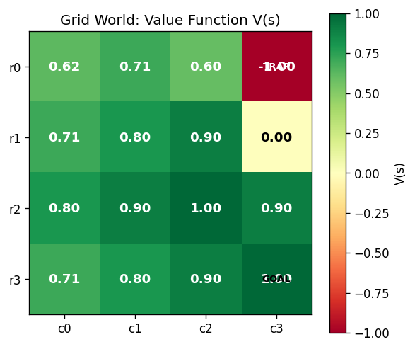
Policy evaluation: compute expected utility (expectation)
\[ V^{\pi}\left(s_{0}\right)=\sum_{t=0}^{h} \gamma^{t} \sum_{s_{t}} \operatorname{Pr}\left(s_{t} | s_{0}, \pi\right) R\left(s_{t}, \pi\left(s_{t}\right)\right) \]This expression corresponds to the policy \(\pi \) when we start in state \(s_0 \)
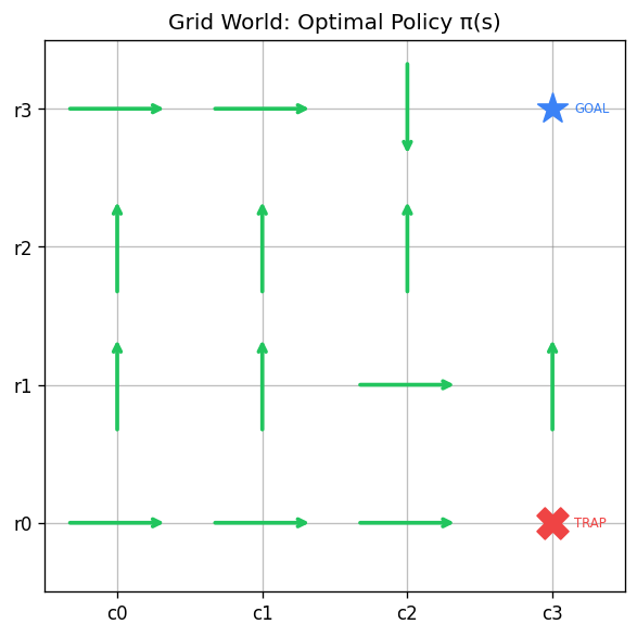
Optimal policy: Policy with highest expected utility
\[ V^{\pi^* } (s_ 0) \ge V^\pi (s_0)\quad \forall \pi \]This is the best policy \(\pi^* \).
Policy Optimization
Several classes of algorithms:
- Value iteration
- Policy iteration
- Linear Programming
- Search techniques
Computation may be done
- Offline: before the process starts, planning ahead
- Online: as the process evolves
Value Iteration
- Performs dynamic programming
- Optimizes decisions in reverse order
Value when no time left:
\[ V(s_ h) = \max_ {a_ h} R(s_ h, a_ h) \]Value with one time step left:
\[ V\left(s_ {h-1}\right)=\max _ {a_ {h-1}} R\left(s_ {h-1}, a_ {h-1}\right)+\gamma \sum_ {s_ {h}} \operatorname{Pr}\left(s_ {h} | s_ {h-1}, a_ {h-1}\right) V\left(s_ {h}\right) \]Value with two time steps left:
\[ V\left(s_ {h-2}\right)=\max _ {a_ {h-2}} R\left(s_ {h-2}, a_ {h-2}\right)+\gamma \sum_{s_ {h-1}} \operatorname{Pr}\left(s_ {h-1} | s_ {h-2}, a_ {h-2}\right) V\left(s_ {h-1}\right) \]…
Bellman’s equation:
\[ \begin{aligned} V\left(s_{t}\right)&=\max _ {a_{t}} R\left(s_ {t}, a_ {t}\right)+\gamma \sum_{s_ {t+1}} \operatorname{Pr}\left(s_{t+1} | s_{t}, a_{t}\right) V\left(s_{t+1}\right) \\ a_{t}^{* }&=\underset{a_ {t}}{\operatorname{argmax}} R\left(s_ {t}, a_ {t}\right)+\gamma \sum_{s_{t+1}} \operatorname{Pr}\left(s_{t+1} | s_{t}, a_{t}\right) V\left(s_{t+1}\right) \end{aligned} \]Finite horizon
- When h is finite,
- Non-stationary optimal policy
- Best action different at each time step
- Intuition: best action varies with the amount of time left
Infinite horizon
- When h is infinite,
- Stationary optimal policy
- Same best action at each time step
- Intuition: same (infinite) amount of time left at each time step, hence same best action
- Problem: value iteration does an infinite number of iterations…
Assuming a discount factor \(\gamma \), after \(n \) time steps, rewards are scaled down by \(\gamma^n \).
For large enough \(n \), rewards become insignificant since \(\gamma^n\to 0 \)
Solution:
- pick large enough \(n \)
- run value iteration for \(n \) steps
- execute policy found at the \(n^{th} \) iteration
Algorithm
Optimal policy \(\pi^* \)
- \(t=0 \): \(\pi_0^* (s) \gets \operatorname{argmax}_a R(s,a)\quad \forall s \)
- \(t>0 \): \(\pi_t^* (s)\gets \underset{a}{\operatorname{argmax}} R(s, a)+\gamma \sum_ {s^{\prime}} \operatorname{Pr}\left(s^{\prime} | s, a\right) V_ {t-1}^{* }\left(s^{\prime}\right)\quad \forall s \)
NB:
- \(t \) indicates the # of time steps to go (till end of process)
- \(\pi^* \) is non stationary (i.e., time dependent)
Matrix form:
- \(R^a \): \(|S |\times 1 \) column vector of rewards for \(a \)
- \(V_t^* \): \(| S |\times 1 \) column vector of state values
- \(T^a \): \(| S | \times | S |\) matrix of transition probability for \(a \)
For infinite horizon, let \(h\to \infty \), then \(V_ h^\pi \to V_ \infty^\pi \)
Policy evaluation:
\[ V_{\infty}^{\pi}(s)=R\left(s, \pi_{\infty}(s)\right)+\gamma \sum_{s^{\prime}} \operatorname{Pr}\left(s^{\prime} | s, \pi_{\infty}(s)\right) V_{\infty}^{\pi}\left(s^{\prime}\right) ~~ \forall s \]Bellman’s equation:
\[ V_{\infty}^{* }(s)=\max_ {a} R(s, a)+\gamma \sum_{s^{\prime}} \operatorname{Pr}\left(s^{\prime} | s, a\right) V_{\infty}^{* }\left(s^{\prime}\right) \]Let’s take a closer look at policy evaluation.
- Linear system of equations
- Matrix form:
- \(R \): \(|S|\times 1 \) column vector of state rewards for \(\pi \)
- \(V \): \(|S|\times 1 \) column vector of state values for \(\pi \)
- \(T \): \(|S|\times |S| \) matrix of transition prob for \(\pi \)
Now we want to solve linear equations. Several ways:
- Gaussian elimination: \((I-\gamma T) V =R\)
- Compute inverse: \(V=(I-\gamma T)^{-1}R \)
- Iterative methods
- value iteration (a.k.a. Richardson iteration)
- repeat \(V\gets R+\gamma T V \)
When we do iteration, the idea is to let the value converge. How do we know it converges?
Let \(H(V) \stackrel{\text { def }}{=} R+\gamma T V \) be the policy eval operator.
\[
    \|H(\tilde V)-H(V)\|_ \infty \le \gamma \| \tilde V - V\|
\]
Proof:
\[ \begin{aligned} || H(\tilde{V})-H(V)|| _ {\infty} &=|| R+\gamma T \tilde{V}-R-\gamma T V|| _ {\infty} \quad \text { (by definition) } \\ &=|| \gamma T(\tilde{V}-V)|| _ {\infty} \quad \text { (simplification) } \\ &\leq \gamma|| T|| _ {\infty}|| \tilde{V}-V|| _ {\infty} \quad \text { (since }\| A B\| \leq\| A\|\| B\|) \\ &=\gamma|| \tilde{V}-V|| _ {\infty} \quad \text { (since } \max _ {s} \sum _ {s^{\prime}} T\left(s, s^{\prime}\right)=1) \end{aligned} \] \[
\lim_ {n\to\infty} H^{(n)}(V) = V^\pi \quad \forall V
\]
Proof omitted or see slides…
In practice, we can’t perform an infinite number of iterations. Suppose that we perform value iteration for \(n \) steps and \(\|H^{(n)}(V)-H^{(n-1)}(V)\|_ \infty=\epsilon \), how far is \(H^{(n)}(V) \) from \(V^\pi \)?
\[
    \|V^\pi - H^{(n)}(V)\|_ \infty \le {\epsilon \over 1-\gamma}
\]
Proof omitted or see slides…
Now let’s take a closer look at optimal value function
- Non-linear system of equations
- Matrix form
- \(R^a \): \(|S|\times 1 \) column vector of state rewards for \(a \)
- \(V^* \): \(|S|\times 1 \) column vector of state values for optimal values
- \(T^a \): \(|S|\times |S| \) matrix of transition prob for \(a \)
Let \(H^* \stackrel{\text { def }}{=} \max_a R^a + \gamma T^a V \) be the operator in value iteration
\[
    \|H^* (\tilde V) - H^* (V)\|_ \infty \le \gamma \|\tilde V - V \|_ \infty
\]
Proof omitted.
\[
    \lim_ {n\to\infty } {H^* }^{(n)} (V) = V^* \quad \forall V
\]
Proof skipped.
Even when horizon is infinite, we perform finitely many iterations. Stop when \(\|V_ n- V_ {n-1}\|_ \infty \le \epsilon \).
Since \(\|V_ n- V_ {n-1}\|_ \infty \le \epsilon \), by Theorem 7, we know that \(\|V_ n- V^* \|_ \infty \le {\epsilon \over 1-\gamma} \). But, how good is the stationary policy \(\pi_n(s) \) extracted based on \(V_n \)?
\[ \pi_{n}(s)=\underset{a}{\operatorname{argmax}} R(s, a)+\gamma \sum_{s^{\prime}} \operatorname{Pr}\left(s^{\prime} | s, a\right) V_{n}\left(s^{\prime}\right) \]How far is \(V^{\pi_ n} \) from \(V^* \)?
\[
    \|V^{\pi_ n} - V^* \|_ \infty \le {2\epsilon \over 1-\gamma}
\]
Proof skipped.
In summary, value iteration is simple DP algorithm with complexity \(O (n |A| |S|^2) \) where \(n \) is the number of iterations.
- Optimize value function
- Extract induced policy
Can we optimize the policy directly instead of optimizing the value function and then inducing a policy?
- Yes: by policy iteration
Policy Iteration
It alternates between two steps
- Policy evaluation
- Policy improvement
until convergence.
Let’s do a comparison:
- Value Iteration:
- Each iteration: \(O(|S|^2 |A|) \)
- Many iterations: linear convergence
- Policy Iteration
- Each iteration: \(O(|S|^3 + |S|^2 |A|) \)
- Few iterations: linear-quadratic convergence, which converges faster
Ideally, we would like a technique which has fewer iterations and smaller cost per iteration.
Modified Policy Iteration
alternates between two steps:
- Partial Policy evaluation, repeat \(k \) times
- Policy improvement
Same convergence guarantees as value iteration. Proof: somewhat complicated (see Section 6.5 of Puterman’s book)
Let’s do a comparison:
- Value Iteration:
- Each iteration: \(O(|S|^2 |A|) \)
- Many iterations: linear convergence
- Policy Iteration
- Each iteration: \(O(|S|^3 + |S|^2 |A|) \)
- Few iterations: linear-quadratic convergence, which converges faster
- Modified Policy Iteration:
- Each iteration: \(O(k|S|^2 + |S|^2 |A|) \)
- Few iterations: linear-quadratic convergence
Intro to RL
Recall MDP, here we are more general in transition model and reward model:
- Transition model: \(Pr(s_ t| s_ {t-1}, a_ {t-1}) \)
- Reward model: \(Pr(r_ t| s_ t, a_ t) \)
which are stochastic instead of being deterministic.
Goal: find optimal policy \(\pi^* \) such that
\[ \pi^* =\operatorname{argmax}_ \pi \sum _ {t=0}^h \gamma^t E _ \pi [r_ t] \]So we can define RL as follows: same thing with MDP, but where we remove transition and reward model (unknown model).
In RL, we are going to learn an optimal policy while interacting with the environment.
Example: Inverted Pendulum
- State: \(x(t), x'(t), \theta(t), \theta'(t) \)
- Action: force \(F \)
- Reward: 1 for any step where pole balanced
Problem: Find \(\pi: S\to A \) that maximizes rewards
Important Components in RL
RL agents may or may not include the following components:
- Model: Environment dynamics and rewards
- Policy: Agent action choices
- Value function: Expected total rewards of the agent policy
Thus, by this, we can categorize RL agents
- Value based: (No policy, implicit.) Value function. If you have a value function, you can always induce a policy just by taking one step of value iteration, and noticing what is the action maximize that step.
- Policy based: Policy, No value function. We can use the rewards given by the environment.
- Actor critic: Policy, value function.
or another way to categorize:
- Model based: Transition and reward model
- Model free: No transition and no reward model (implicit)
Model free evaluation
Given a policy \(\pi \), estimate \(V^\pi(s) \) without any transition or reward model.
- Monte Carlo evaluation (sample approximation)
- Temporal difference (TD) evaluation (one sample approximation)
Monte Carlo Evaluation
Let’s look more closely at Monte Carlo Evaluation.
Let \(G_k \) be a one-trajectory Monte Carlo target
\[ G_ k = \sum_ t\gamma^t r_t^{(k)} \]Approximate value function
\[ \begin{aligned} V_{n}^{\pi}(s) & \approx \frac{1}{n(s)} \sum_{k=1}^{n(s)} G_{k} \\ &=\frac{1}{n(s)}\left(G_{n(s)}+\sum_{k=1}^{n(s)-1} G_{k}\right) \\ &=\frac{1}{n(s)}\left(G_{n(s)}+(n(s)-1) V_{n-1}^{\pi}(s)\right) \\ &=V_{n-1}^{\pi}(s)+\frac{1}{n(s)}\left(G_{n(s)}-V_{n-1}^{\pi}(s)\right) \end{aligned} \]Incremental update
\[ V_ n^\pi(s)\gets V_{n-1}^{\pi}(s)+\underbrace{\alpha_ n}_ {\text{learning rate } 1/n(s)}\left(G_{n(s)}-V_{n-1}^{\pi}(s)\right) \]Temporal Difference Evaluation
Then look at Temporal Difference Evaluation. Its approximate value function is
\[ V^\pi (s) \approx r+ \gamma V^\pi(s') \]Incremental update:
\[ V_{n}^{\pi}(s) \leftarrow V_{n-1}^{\pi}(s)+\alpha_{n}\left(r+\gamma V_{n-1}^{\pi}\left(s^{\prime}\right)-V_{n-1}^{\pi}(s)\right) \]Sufficient conditions for \(\alpha_n \)
- \(\sum_ n\alpha_ n \to\infty \)
- \(\sum_ n(\alpha_ n)^2< \infty \)
Often \(\alpha_ n(s)= 1/n(s) \), where \(n(s) = \) # of times \(s \) is visited.
Comparison
- Monte Carlo evaluation:
- Unbiased estimate
- High variance
- Needs many trajectories
- Temporal difference evaluation:
- Biased estimate
- Lower variance
- Needs less trajectories
Model Free Control
Instead of evaluating the state value function, \(V^\pi(s) \), evaluate the state-action value function, \(Q^\pi(s,a) \)
- it is value of executing \(a \) followed by \(\pi \)
- \(Q^{\pi}(s, a)=E[r | s, a]+\gamma \sum_ {s^{\prime}} \operatorname{Pr}\left(s^{\prime} | s, a\right) V^{\pi}\left(s^{\prime}\right) \)
Greedy policy \(\pi' \): \(\pi'(s)=\operatorname{argmax}_ aQ^\pi(s,a) \)
Based on this, we can define Bellman’s eq w.r.t. Q function
- Optimal state value function
- Optimal state-action value function
where \(V^* (s) = \max_a Q^* (s,a ) \) and \(\pi^* (s) =\operatorname{argmax}_ a Q^* (s,a) \).
The main difference is we move max from the beginning to the end of the eqn, but that doesn’t change the math really. These two eqns are mathematically equivalent.
Monte Carlo Control
Temporal Difference Control
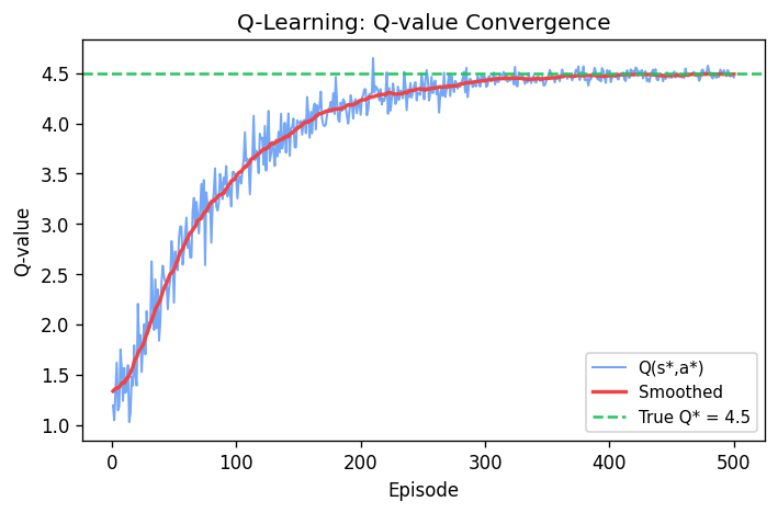
Q learning
but how we select action?
Exploration vs Exploitation
- If an agent always chooses the action with the highest value then it is exploiting
- The learned model is not the real model
- Leads to suboptimal results, might stuck to a local optimum
- By taking random actions (pure exploration) an agent may learn the model
- But what is the use of learning a complete model if parts of it are never used?
- Need a balance between exploitation and exploration
Common exploration methods
- \(\epsilon \)-greedy
- with probability \(\epsilon \) execute random action
- Otherwise execute best action \(a^* = \operatorname{argmax}_ a Q(s,a)\)
- Boltzmann exploration
Q-learning converges to optimal Q-values if
- Every state is visited infinitely often (due to exploration)
- The action selection becomes greedy as time approaches infinity
- The prob of exploration \(\epsilon \) is decreased fast enough, but not too fast (similar like learning rate \(\alpha \) previously)
Deep Neural Networks
Like in computer go, we have large state spaces.
Functions to be approximated:
- Policy: \(\pi(s)\to a \)
- Q-function: \(Q(s,a)\in\mathfrak R \)
- Value function: \(V(s)\in\mathfrak R \)
We need to approximate them and we can’t use tables or vectors for them. Let’s focus on Q-function. In the future lectures, we might focus other functions afterwards.
Let \(s=(x_ 1, x_ 2,\ldots, x_ n)^T \), a set/vector of features. Then we take a linear combination with weights:
\[ Q(s,a) \approx \sum_ i w _ {ai}x _ i \]or non-linear (e.g., neural network): \(Q(s,a)\approx g({\bf x}; {\bf w}) \)
For the rest of this part, please consult lecture 4a.
Mitigating Vanishing Gradients
Some popular solutions:
- Pre-training
- Rectified linear units
- Batch normalization
- Skip connections
Rectified Linear Units
Rectified linear: \(h(a)=\max(0,a) \)
- gradient is 0 or 1
- sparse computation since not smooth
Soft version (“Softplus”): \(h(a)=\log (1+e^a) \)
Warning: softplus does not prevent gradient vanishing (gradient < 1)
So softplus looks like a good idea, but it’s not, didn’t mitigate gradient vanishing problem. So you really want to use rectified linear units. Not smooth is not a big deal, because you can use subgradient techniques to do the optimization.
Deep Q-networks
Q-function Approximation
- Let \(s=(x_ 1, \ldots, x_ n)^T \)
- Linear \(Q(s, a) \approx \sum_ i w_ {ai} x_ i \)
- Non-linear (e.g., neural network): \(Q(s,a) \approx g({\bf x}; {\bf w}) \)
Gradient Q-learning
Minimize squared error between Q-value estimate and target
- Q-value estimate: \(Q_{\bf w}(s,a) \)
- Target: \(r+\gamma \max_ {a'} Q _ {\overline{\bf w}}(s', a') \)
Squared error:
\[ Err({\bf w}) = {1\over 2} \left[Q_ {\bf w}(s, a) -r - \gamma \max_ {a'} Q_ {\overline {\bf w}} (s', a') \right]^2 \]where \(\overline {\bf w} \) is fixed.
Gradient:
\[ {\partial Err \over \partial {\bf w}} = \left[ Q_ {\bf w}(s, a) - r - \gamma \max_ {a'} Q_ { \overline {\bf w}} (s', a')\right] {\partial Q_ {\bf w}(s,a)\over \partial {\bf w}} \]Historically, there was just one network, and we didn’t use \(\overline{\bf w} \). It sometimes works, sometimes diverges. Now we use two networks, one for main estimate, one for target. Keep target network fixed and simply update the other network, then it will get rid of the problem.
We find that even if we don’t fix w, if we satisfy the conditions, it will converge.
Even when the following conditions hold, non-linear gradient Q-learning may diverge. The fact is that we didn’t fix w then the target is shifting, then not be able to converge.
Intuition: adjusting w to increase \(Q \) at \((s,a) \) might introduce errors at nearby state-action pairs.
Mitigating divergence
Two tricks are often used in practice
- Experience replay
- Use two networks:
- Q-network
- Target network
Experience Replay
Idea: store previous experiences \(s,a,s',r \) into a buffer and sample a mini-batch of previous experiences at each step to learn by Q-learning
Advantages
- Break correlations between successive updates (more stable learning)
- Fewer interactions with environment needed to converge (greater data efficiency)
Target Network
Idea: Use a separate target network that is updated only periodically
repeat for each \(s,a,s',r \) in mini-batch:
\[ \begin{aligned} {\bf w}&\gets {\bf w} -\alpha_t \left[\underbrace{Q_ {\bf w}} _ {update} - r - \gamma \max _ {a'} \underbrace{ Q_ {\overline {\bf w}} (s',a')} _ {target} \right] {\partial Q_ {\bf w} (s,a) \over \partial {\bf w}}\\ \overline {\bf w} &\gets {\bf w} \end{aligned} \]Advantage: mitigate divergence
It is similar to value iteration: repeat for all \(s \). We have contraction mapping which guarantees it to converge.
Deep Q-network
Proposed by Google Deep Mind. It is Gradient Q-learning with
- Deep neural networks
- Experience replay
- Target network
Breakthrough: human-level play in many Atari video games
Policy Gradient Methods
- Model-free policy-based method
- No explicit value function representation
Ezist policy is Stochastic Policy. Consider stochastic policy \(\pi_ \theta (a| s)= Pr(a|s;\theta ) \) parametrized by \(\theta \). Continuous function.
Finitely many discrete actions. Softmax, quite popular in neural networks.
Softmax: \(\pi_ \theta (a| s) = {\exp{h(s,a;\theta)}\over \sum_ {a'} \exp{h(s,a';\theta)}} \) where \(h(s,a;\theta) \) might be (we can think of it as a scoring function)
- linear in \(\theta \): \(h(s,a;\theta)=\sum_ i\theta _ i f _ i (s,a) \). \(f_ i \)’s are basis functions.
- or non-linear in \(\theta \): \(h(s,a;\theta) = neuralNet(s,a;\theta) \).
Continuous actions: a distribution.
- Gaussian: \(\pi_ \theta (a|s) = N(a| \mu (s;\theta), \sum (s;\theta)) \)
Before policy gradients, take a step back, look at supervised learning. Consider a stochastic policy \(\pi_ \theta (a|s) \). We have data: state-action pairs where actions are optimal for each state:
\[ \left\{ (s_ 1, a_ 1^* ), (s _ 2, a _ 2 * ),\ldots \right\} \]Then we maximize log likelihood of the data:
\[ \theta^* = \operatorname{argmax}_ \theta \sum _ n \log \pi _ \theta ( a_ n ^ * | s _ n) \]and gradient update:
\[ \theta _ {n+1} \gets \theta _ n + \alpha _ n \nabla _ \theta \log \pi _ \theta ( a_ n ^ * | s _ n) \]Let’s compare that with RL. We will have a stochastic policy \(\pi _ \theta (a|s) \). The difference is we don’t know which is the best one for every state. Instead, we have state-action-reward triples: the action we have tried and the reward, and we don’t know if it’s the best one.
\[ \left\{ (s _ 1, a _ 1, r _ 1),\ldots \right\} \]So we try to maximize discounted sum of rewards, expectation of future rewards:
\[ \theta^* = \operatorname{argmax}_ \theta \sum _ n \gamma ^ n E _ \theta [r _ n| s _ n, a _ n] \]Gradient update:
\[ \theta _ {n+1}\gets \theta _ n + \alpha _ n \gamma ^ n G _ n \nabla _ \theta \log \pi _ \theta ( a _ n | s _ n) \]where \(G_ n =\sum _ {t=0}^\infty \gamma^t r _ {n+t} \). Monte Carlo estimate for the sum of discounted reward for one trajectory.
It looks like supervised learning, but it is hard to derive. To derive this, we introduce a theorem.
\(\mu _ \theta (s) \): stationary state distribution when executing policy parametrized by \(\theta \).
\(Q_ \theta (s,a) \): discounted sum of rewards when starting \(s \), executing \(a \) and following the policy parametrized by \(\theta \) thereafter.
Derivation skipped…
Based on this theorem, we can drop the summation, and approximation by samples (Monte Carlo Policy Gradient).
\[ \nabla V _ \theta \propto \ldots = E _ \theta [\gamma ^n G_ n \nabla \log \pi _ \theta ( A _ n | S _ n)] \]When we drop expectation, we can get one sample approximation, which corresponds to Stochastic gradient descent: \(\nabla V _ \theta \approx \gamma ^n G_ n \nabla \log \pi _ \theta ( A _ n | s _ n) \).
This alg is quite old, one of the early RL techniques.
Computer Go. Winning strategy, four steps:
- Supervised Learning of Policy Networks
- Policy gradient with Policy Networks
- Value gradient with Value Networks
- Searching with Policy and Value Networks
Actor Critic Algorithms
- Q-learning
- Model-free value-based method
- No explicit policy representation
- Policy gradient
- Model-free policy-based method
- No explicit value function representation
- Actor Critic
- Model-free policy and value based method
Baseline often chosen to be \(b(s)\approx V^\pi (s) \).
Advantage function: \(A(s,a) = Q(s,a) - V^\pi (s) \). How much Q function differs from the value function?
Gradient update:
\[ \theta \gets \theta \alpha \gamma^n A (s_ n, a_ n) \nabla \log \pi_ \theta (a _ n | s _ n) \]Benefit: faster empirical convergence
If we look at the code, we now have both a value function and a policy.
Instead of updating \(V(s) \) by Monte Carlo sampling, where we need to wait for a complete episode and get entire trajectory, not sample efficient. What is better, we can do bootstrap with temporal difference updates. So we don’t need to wait until the end.
\[ \delta \gets r_ n + \gamma V_ w(s _ {n+1})- V_ w(s _ n) \]Benefit: reduced variance (faster convergence)
This leads actor critic.
Instead of doing temporal difference updates, update with the advantage function (see algorithm below)
Benefit: faster convergence
This leads to Advantage Actor Critic (A2C). Also Asynchronous Advantage Actor Critic (A3C) algorithm. It turns out asynchronous fashion is not critical…
Continuous actions. Now we have discussed stochastic policy. What if we want a policy that is deterministic? Consider a deterministic policy \(\pi_ \theta (s)\to a \)
\[
    \nabla V_{\theta}\left(s_{0}\right) \propto E_{s \sim \mu_{\theta}(s)}\left[\left.\nabla_{\theta} \pi_{\theta}(s) \nabla_{a} Q_{\theta}(s, a)\right|_{a=\pi_{\theta}(s)}\right]
\]
Proof: see Silver et al. 2014
So this leads to Deterministic Policy Gradient. In some literatures, we have DDPG (deep …) which is encoded in neural networks. This is actually actor-critic technique, with explicit Q-function, policy and we do updates for both of them.
Trust Region Methods
It is common to formulate ML problems as optimization problems.
- Min squared error
- Min cross entropy
- Max log likelihood
- Max discounted sum of rewards
There are two important classes:
- Line search methods
- Find a direction of improvement
- Select a step length
- Trust region methods
- Select a trust region (analog to max step length)
- Find a point of improvement in the region
Idea: approximate obj \(f \) with a simpler obj \(\tilde f \) and solve \(\tilde x^* = argmin_x \tilde f(x) \)
Problem: The optimum \(\tilde x^* \) might be in a region where \(\tilde f \) poorly approximates \(f \) and \(\tilde x^* \) might be far from optimal
Solution: restrict the search to a region where we trust \(\tilde f \) to approximate \(f \) well.
For example, \(\tilde f \) often chosen to be a quadratic approx of \(f \)
\[ \begin{aligned} f(x)&\approx \tilde f(x) \\ &= f(c) + \nabla f(c)^T (x-c) + {1\over 2!}(x-c)^T H(c)(x-c) \end{aligned} \]where \(\nabla f \) is the gradient and \(H \) is the hessian. Trust region often chosen to be a hypersphere \(||x-c ||_ 2\le \delta \)
Generic algorithm: alternate between solving opt (trust region subproblem) and adjusting region size. Repeat until convergence.
When \(H \) is positive semi-definite, we get a convex opt, which gives us simple and globally optimal solution. When \(H \) is not PSD, it’s non-convex optimization, simple heuristics that guarantee improvement.
Trust Region Policy Optimization
Recall policy gradient, \(\alpha \) (learning rate) is difficult to set:
- small: slow but reliable convergence
- big: fast but reliable
Trust region method
We often optimize a surrogate (替代) objective (approximation of \(V \). Surrogate objective may be trustable (close to \(V \) only in a small region. Limit search to small trust region.
Let \(\theta \) be the parameters for policy \(\pi _ \theta (s|a) \). We can define a region around \(\theta \) or around \(\pi_ \theta \). \(V \) often varies more smoothly with \(\pi_ \theta \) than \(\theta \). Hence define policy trust regions.
Kullback-Leibler Divergence. Intuition: expectation of the log diff between \(p \) and \(q \),
\[ D _ {K L}(p, q)=\sum _ {x} p(x) \log \frac{p(x)}{q(x)} \]Trust region policy optimization. Update step:
\[ \begin{aligned} \theta \leftarrow & \underset{\widetilde{\theta}}{\operatorname{argmax}} E_{s_{0} \sim p}\left[V^{\pi_{\tilde{\theta}}}\left(s_{0}\right)-V^{\pi_{\theta}}\left(s_{0}\right)\right] \\ & \text { subject to } \max _{\mathrm{s}} D_{K L}\left(\pi_{\theta}(\cdot \mid s), \pi_{\widetilde{\theta}}(\cdot \mid s)\right) \leq \delta \end{aligned} \]Since the objective is not directly computable, let’s approximate it:
\[ \underset{\widetilde{\theta}}{\operatorname{argmax}} E_{s_{0} \sim p}\left[V^{\pi_{\tilde{\theta}}}\left(s_{0}\right)-V^{\pi_{\theta}}\left(s_{0}\right)\right] \approx \underset{\widetilde{\theta}}{\operatorname{argmax}} E_ {s\sim \mu _ \theta, a \sim \pi _ \theta} \left[{\pi _ {\tilde\theta (a | s)\over \pi _ \theta ( a| s)}} A _ \theta (s,a) \right] \]where \(\mu_ \theta (s) \) is the stationary state distribution for \(\pi \).
Let’s also relax the bound on the max KL-divergence to a bound on the expected KL-divergence, which is relaxed to expectation
\[ E_ {s\sim \mu _ \theta} [D _ {KL} \left( \pi _ \theta (\cdot | s), \pi _ {\tilde \theta} ( \cdot | s) \right)] \]Derivation skipped.
Trust Region Policy Optimization (TRPO). Most of the algorithm is identical to actor-critic. Difference is update to the actor as we mentioned before.
One drawback is the complexity of optimization. In practice, obj is approximated with linear function and constraint is approximated with a quadratic function.
TRPO is conceptually and computationally challenging in large part because of the constraint in the optimization. The effect of the constraint: effectively constraining the ratio \({\pi _ \theta (a|s) \over \pi_ {\tilde \theta} (a | s)} \).
Therefore, let’s design a simpler objective that directly constrains \({\pi _ \theta (a|s) \over \pi_ {\tilde \theta} (a | s)} \). We are going to clip the ratio.
We can use this simpler objective to define a new alg called Proximal Policy Optimization (PPO).
See details in slides.
Maximum Entropy Reinforcement Learning
First, let’s compare deterministic policies and stochastic policies.
Deterministic
- There always exists an optimal deterministic policy
- Search space is smaller for deterministic than stochastic policies
- Practitioners prefer deterministic policies
Stochastic
- Search space is continuous for stochastic policies (helps with gradient descent)
- More robust (less likely to overfit)
- Naturally incorporate exploration
- Facilitate transfer learning
- Mitigate local optima
Based on standard MDP, we add entropy term to encourage stochasticity. Let reward: \(R(s,a) + \lambda H( \pi (\cdot | s)) \)
Entropy: measure of uncertainty.
\[ H(p) = -\sum_ x p(x) \log p (x) \]Accordingly, we change our policy function and value function to get several soft versions.
Soft Q-learning:
- Q-learning based on Soft Q-Value Iteration
- Replace expectations by samples
- Represent Q-function by a function approximator (e.g., neural network)
- Do gradient updates based on temporal differences
In practice, actor critic techniques tend to perform better than Q-learning. Can we derive a soft actor-critic algorithm?
Yes. Critic: soft Q-function. Actor: (greedy) softmax policy.
Soft Actor-Critic
- RL version of soft policy iteration
- Use neural networks to represent policy and value function
- At each policy improvement step, project new policy in the space of parameterized neural nets
See the pseudocodes and math derivation in slides.
Multi-armed bandits
It is really is RL with single state.
Exploration/Exploitation Tradeoff
Fundamental problem of RL due to the active nature of the learning process. When you consider ML in general, like supervised/unsupervised learning, there is no exploration: just feed the data to predictor. In RL, you have to be active to select an action when at some state, and has influence in the future. Now consider one-state RL problems known as bandits.
No transition function to be learned since there is a single state. We simply need to learn the stochastic reward function.
The term bandit comes from gambling where slot machines can be thought as one-armed bandits.
Problem: which slot machine should we play at each turn when their payoffs are not necessarily the same and initially unknown?
In practice, there are some examples that can be formed as bandit:
- Design of experiments (Clinical Trials) in health or biology
- Online ad placement
- Web page personalization
- Games
- Networks (packet routing)
Online Ad Optimization
Problem: which ad should be presented?
Answer: present ad with highest payoff
payoff = clickThroughRate × payment
- Click through rate: probability that user clicks on ad
- Payment: $$ paid by advertiser
- Amount determined by an auction
Introduced by Google yrs ago.
Now let’s simplify the problem:
- Assume payment is 1 unit for all ads
- Need to estimate click through rate
Formulate as a bandit problem:
- Arms: the set of possible ads
- Rewards: 0 (no click) or 1 (click)
In what order should ads be presented to maximize revenue? How should we balance exploitation and exploration?
Simple yet difficult problem
- Simple: description of the problem is short
- Difficult: no known tractable optimal solution
Simple heuristics
- Greedy strategy: select the arm with the highest average so far.
- May get stuck due to lack of exploration
- \(\epsilon \)-greedy: select an arm at random with
probability \(\epsilon \) and otherwise do a greedy selection
- Convergence rate depends on choice of \(\epsilon \)
Regret
Let \(R(a) \) be the unknown average reward of \(a \).
Let \(r^* = \max_ a R(a) \) and \(a^* =\operatorname{argmax} _ aR(a) \)
Denote by \(loss(a) \) be the expected regret of \(a \), for each action
\[ loss(a)= r^* - R(a) \]Denote \(Loss_ n \) the expected cumulative regret for \(n \) time steps
\[ Loss_ n = \sum _ {t=1}^n loss(a_ t) \]When \(\epsilon \) is constant, then
- For large enough \(t \): \(Pr(a _ t \ne a^* ) \approx \epsilon \)
- Expected cumulative regret: \(Loss _ n \approx \sum_ {t=1}^n \epsilon = O(n) \). Linear regret
When \(\epsilon_ t\propto 1/t \). Choose it to decrease.
- For large enough \(t \): \( Pr(a _ t \ne a^* ) \approx \epsilon_ t = O(1/t )\)
- Expected cumulative regret: \(Loss _ n = \sum _ {t=1}^n {1\over t}= O(\log n) \). Logarithmic regret.
Empirical mean
Problem: how far is the empirical mean \(\tilde R(a) \) from the true mean \(R(a) \)?
If we knew that \(|R(a)-\tilde R(a)|\le bound \)
- Then we wound know that \(R(a)< \tilde R(a)+bound \)
- And we could select the arm with best \(\tilde R(a)+ bound \)
Overtime, additional data will allow us to refine \(\tilde R(a) \) and compute a tighter bound
Suppose that we have an oracle that returns an upper bound \(UB_ n(a) \) on \(R(a) \) for each arm based on \(n \) trials of arm \(a \).
Suppose the upper bound returned by this oracle converges to \(R(a) \) in the limit. Then we can develop optimistic algorithm: At each step, select \(\operatorname{argmax}_ a UB_ n (a) \)
Proof by contradiction.
Problem: We can’t compute an upper bound with certainty since we are sampling. However, we can obtain measures \(f \) that are upper bounds most of the time
- i.e., \(Pr(R(a)\le f(a)) \ge 1-\delta \)
- Example: Hoeffding’s ineq:
where \(n _ a \) is the number of trials for arm \(a \)
Upper Confidence Bound (UCB)
Set \(\delta_n = {1\over n^4} \) in Hoeffding’s bound. CHoose \(a \) with highest Hoeffding bound
Idea: As \(n \) increases, the term \(\sqrt{2\log n \over n _ a} \) increase, ensuring that all arms are tried infinitely often
Expected cumulative regret is logarithmic regret.
Summary
- Stochastic bandits
- Exploration/exploitation tradeoff
- \(\epsilon \)-greedy and UCB
- Theory: logarithmic expected cumulative regret
- In practice:
- UCB often performs better than \(\epsilon \)-greedy
- Many variants of UCB improve performance
Bayesian
Previously, we examined \(\epsilon \)-greedy and UCB. There are alternative Bayesian approaches: Thompson sampling and Gittins indices.
Bayesian Learning
Notation:
- \(r^a \): random variable for \(a \)’s rewards
- \(Pr(r^a;\theta) \): unknown distribution (parametrized by \(\theta \)
- \(R(a)= E[r^a] \): unknown avg reward
Idea:
- Express uncertainty about \(\theta \) by a prior \(Pr(\theta) \)
- Compute posterior \(Pr(\theta| r_ 1^a, \ldots , r _ n^a) \) based on samples \(r_ 1 ^a,\ldots, r_ n^a \) observed for \(a \) so far.
By Bayes theorem:
\[ Pr(\theta| r_ 1^a, \ldots , r _ n^a) \propto Pr(\theta) Pr (r_ 1^a,\ldots, r_ n^ a| \theta ) \]Posterior over \(\theta \) allows us to estimate
- Distribution over next reward \(r^a \)
- Distribution over \(R(a) \) when \(\theta \) includes the mean
To guide exploration:
- UCB: \(Pr(R(a)\le bound (r_ 1^a, \ldots, r _ n^a))\ge 1-\delta \)
- Bayesian techniques: \(Pr(R(a)| r_ 1^a, \ldots , r _ n^a) \)
Now consider coin example. Consider two biased coin \(C_ 1 \) and \(C _ 2 \)We want to maximize # of heads in \(k \) flips. Which coin should we choose for each flip?
\(r^{C _ 1}, r^{C _ 2} \) are Bernoulli vars with domain \(\left\{ 0,1 \right\} \). Bernoulli distribution are parametrized by their mean.
Here we let the prior \(Pr(\theta) \) be a Beta distribution:
\[ Beta(\theta,\alpha, \beta)\propto \theta^{\alpha-1}(1-\theta)^{\beta-1} \]Here \(\alpha-1 \) is # of heads, \(\beta-1 \) is # of tails. Then \(E(\theta)=\alpha/(\alpha+\beta) \).
Prior: \(Pr(\theta) = Beta(\theta; \alpha,\beta)\propto \theta^{\alpha-1}(1-\theta)^{\beta-1} \)
Posterior after coin flip:
- \(Pr(\theta|head) \propto Beta(\theta;\alpha+1,\beta) \)
- \(Pr(\theta|head) \propto Beta(\theta;\alpha,\beta+1) \)
Thompson Sampling
Idea:
- Sample several potential average rewards for each \(a \)
- Estimate empirical average
- Execute \(\operatorname{argmax}_a \hat R(a) \)
Thompson Sampling Algorithm Bernoulli Rewards
Comparison
Note that on the left, \(i \) means the index of samples that I get from posterior distribution; on the right, it means time step.
In Thompson sampling, amount of data \(n \) and sample size \(k \) regulate amount of exploration
As \(n \) and \(k \) increases, \(\hat R(a) \) becomes less stochastic, which reduces exploration
- As \(n \) increases, \(Pr( R(a) | r_ 1^a,\ldots, r_ n^a) \) becomes more peaked
- As \(k \) increases, \(\hat R(a) \) approaches \(E[R(a)| r_ 1^a, \ldots, r _ n^a] \)
The stochasticity of \(\hat R(a) \) ensures that all actions are chosen with some probability.
Thus we can show that Thompson sampling converges to best arm. In theory, expected cumulative regret: \(O(\log n) \), which is on par with UCB and \(\epsilon \)-greedy. In practice: we choose sample size \(k \) often to be 1. It is small because
- computationally faster
- ensure that there is more exploration
Contextual Bandits
In many applications, the context provides additional information to select an action. Select action based on contexts.
- E.g., personalized advertising, user interfaces
- Context: user demographics (location, age, gender)
Actions can also be characterized by features that influence their payoff
- E.g., ads, webpages
- Action features: topics, keywords, etc
Contextual bandits: multi-armed bandits with states (corresponding to contexts) and action features
Formally:
- \(S \): set of states where each state \(s \) is defined by a vector of features \({\bf x}^s = (x_ 1^s,\ldots, x_ k^s) \)
- \(A \): set of actions where each action \(a \) is associated with a vector of features \({\bf x}^a = (x_ 1^a, \ldots, x_ \ell ^a) \)
- Space of rewards (often \(\mathbb R \)
Still, no transition function since the states at each step are independent. No correlations between each state.
Goal: find policy \(\pi:{\bf x}^S\to a \) that maximizes expected rewards \(E(r|s,a)=E(r|{\bf x}^S, {\bf x}^a) \)
A common approach is to learn approximate average reward function \(\tilde R(s,a)=\tilde R({\bf x})=\tilde R({\bf x}^s,{\bf x}^a) \) by regression. To approximate it, we have linear/non-linear approximation as before.
The rest of math modelling can be found in lecture 8b:
- Bayesian Linear Regression: find best set of weights that explain how to obtain the rewards by a linear combo of the input features
- Predictive Posterior: With Gaussian distribution, we impose a bound with certain probability. The derivation would require knowledge from probability and statistics.
Then we put these into an algorithm: Upper Confidence Bound (UCB) Linear Gaussian.
Thompson Sampling Algorithm Linear Gaussian
Industrial Use
Contextual bandits are now commonly used for
- Personalized advertising
- Personalized web content
- MSN news: 26% improvement in click through rate after adoption of contextual bandits
Model-based RL
Learn explicit transition and/or reward model
- plan based on the model
- benefit: increased sample efficiency
- drawback: increased complexity
Idea: at each step
- Execute action
- Observe resulting state and reward
- Update transition and/or reward model
- Update policy and/or value function
Model-based RL (with Value Iteration)
Complex models
Use function approx. for transition and reward models
- Linear model
- Non-linear models:
- Stochastic (e.g., Gaussian process)
- Deterministic (e.g., neural network)
In complex models, fully optimizing the policy or value function at each time step is intractable. Thus consider partial planning
- A few steps of Q-learning
- A few steps of policy gradient
Model-based RL (with Q-learning)
Partial Planning vs Replay Buffer
Previous algorithm is very similar to Model-free Q-learning with a replay buffer. Instead of updating Q-function based on samples from replay buffer, generate samples from model
- Replay buffer:
- Simple, real samples, no generalization to other sate-action pairs
- Partial planning with a model
- Complex, simulated samples, generalization to other state-action pairs (can help or hurt)
Dyna
Learn explicit transition and/or reward model. Plan based on the model
Learn directly from real experience
Instead of planning at arbitrary states, plan from the current state. This helps improve next action. Monte Carlo Tree Search.
The idea: we can build a search tree. It will grow exponentially.
The question: if we do planning from current state, how tractablly? not to build the entire search tree. Three ideas:
- Leaf nodes: approximate leaf values with value of default policy \(\pi \). Give us an estimate and cut off the search.
- Chance nodes: approximate expectation by sampling from transition model. Take the sample of the children.
- Decision nodes: expand only most promising actions
If we combine these three ideas, the resulting algorithm: Monte Carlo Tree Search
Monte Carlo Tree Search
(with upper confidence bound)
\(node_ \ell \) indicates the leaf.
See the helper functions in lecture 9.
Note that in two player mode, one try to minimize, the other one try to maximize the score.
In AlphaGo, four steps:
- Supervised Learning of Policy Networks
- Policy gradient with Policy Networks
- Value gradient with Value Networks
- Searching with Policy and Value Networks
- Monte Carlo Tree Search variant
Bayesian RL
This topic is really exciting. None of the textbooks cover it. Reading: Michael O’Gordon Duff’s PhD Thesis (2002). For this lecture, we will only talk about model-based Bayesian RL.
So far, we have seen model-free and model-based RL.
- Model-free RL: unbiased direct learning, needs many interactions with environment
- Model-based: biased indirect learning via a model, if bias is not too important then less data needed
With a model-based approach, the issue is biased model. Problem:
- Model learned from finite amount of data
- Model is necessarily imperfect
- There is a risk that planning will overfit the model inaccuracies and produce a bad policy
Solution: represent uncertainty in model
We are going to model uncertainty, where we have a distribution over possible models.
Bayesian RL
- Explicit representation of uncertainty
- Benefits
- Balance exploration/exploitation tradeoff
- Mitigate model bias
- Reduce data needs
- Drawback
- Complex computation
In Bayesian RL, idea: augment state with distribution about unknown parameters
- Information states: \((\boldsymbol s, \boldsymbol b \in \boldsymbol S\times B) \)
- Physical states: \(\boldsymbol s\in \boldsymbol S \)
- Belief states: \(\boldsymbol b\in \boldsymbol B \) where \(b(\theta) = Pr(\theta) \). If certain, distribution will be quite peak. Otherwise, quite wide.
- Actions: \(\boldsymbol a\in \boldsymbol A \)
- Rewards: \(\boldsymbol r\in\mathbb R \)
- Known model: \(Pr(\boldsymbol r,\boldsymbol s',\boldsymbol b'| \boldsymbol s, \boldsymbol b, \boldsymbol a) \)
Goal: find policy \(\pi:S\times B\to A \) and/or value function \(Q:S\times B\times A\to \mathbb R \)
Now let’s look more closely at the model since we claim the model in Bayesian RL is know!
\[ \operatorname{Pr}\left(r, s^{\prime}, b^{\prime} | s, b, a\right)= \underbrace{\operatorname{Pr}\left(r, s^{\prime} | s, b, a\right) } _ {\text{Physical model}} \underbrace{\operatorname{Pr}\left(b^{\prime} | r, s^{\prime}, s, b, a\right)} _ {\text{belief model}} \]Idea:
- For physical, integrate out unknown \(\theta \)
- For belief, \(b' \) is the posterior belief
Belief state
Let’s model our uncertainty with respect to \(\theta \) by a Beta distribution
\[ b(\theta) =k\theta^{\alpha-1}(1-\theta)^{\beta-1} \]Belief Update: Bayes theorem
\[ \begin{aligned} b^{\prime}(\theta) &=b^{s, a, s^{\prime}}(\theta) \\ &=b\left(\theta | s, a, s^{\prime}\right) \\ & \propto b(\theta) \operatorname{Pr}\left(s^{\prime} | s, a, \theta\right) \end{aligned} \]Physical Model
Consider \(s=(i,j) \), \(a=right \), \(s'=(i',j') \) where \(i'=i \) and \(j' = j-1 \).
Predictive distribution
\[ \begin{aligned} \operatorname{Pr}\left(s^{\prime} | s, b, a\right) &=\int _ {\theta} \operatorname{Pr}\left(s^{\prime} | s, a, \theta\right) b(\theta) d \theta \\ &=\int _ {\theta} \operatorname{Pr}\left(i^{\prime}, j^{\prime} | i, j, right, \theta\right) \operatorname{Beta}(\theta ; \alpha, \beta) d \theta \\ &=\int _ {\theta} \frac{(1-\theta)}{2} k \theta^{\alpha-1}(1-\theta)^{\beta-1} d \theta \\ &= {\beta \over 2(\alpha + \beta)} \end{aligned} \]Planning
Since the model is known, treat Bayesian RL as an MDP.
Benefits:
- Solve RL problem by planning (e.g., value/policy iteration)
- Optimal exploration/exploitation tradeoff. We can see this via Bellman’s Equation (augment \(s \) with \(b \) for each occurrence)
Drawback: Complex computation
Then we have only one single objective: max expected total rewards
- \(V^\pi(s,b)=\sum _ t \gamma^t E[r _ t s _ t, b _ t] \).
- Optimal policy \(\pi^* \)
- Optimal exploration/exploitation tradeoff (given prior knowledge)
Two phases:
Challenges
Offline planning is notoriously difficult
- Use function approximators (e.g., Gaussian process or neural net) for model, !∗ and #∗
- Continuous belief space
- Problem: a good plan should implicitly account for all possible environments, which is intractable
Alternative: online partial planning
- Thompson sampling
- PILCO (Model-based Bayesian Actor Critic)
Thompson Sampling in Bayesian RL
Idea: Sample models \(\theta_i \) at each step and plan for the corresponding \(MDP_ {\theta_ i} \)’s
Model-based Bayesian Actor Critic
Second approach
PILCO: Deisenroth, Rasmussen (2011). Deep PILCO: Gal, McCallister, Rasmussen (2016), replace Gaussian process transition model (\(b\theta \) by Bayesian neural network transition model
Unprecedented Data Efficiency
Hidden Markov Models
This is the context of partial observability.
Recall our problem, why can we assume the environment reveals the state completely? Instead, the environment provides observation: some info, but might be complete. This is a more general setting.
Goal: Learn to choose actions that maximize rewards
Recall Markov Process
- first-order Markovian
- Stationary
Hidden Markov Model: instead of having process with states, we are going to create observations correlated with states. Assumptions:
- first-order Markovian
- Stationary
Examples: speech recognition, mobile robot localisation.
Mobile Robot Localisation
- \(s \): coordinates of the robot on a map
- \(o \): distances to surrounding obstacles (measured by laser range finders or sonars)
- \(Pr(s_ t| s_ {t-1}) \): movement of the robot with uncertainty
- \(Pr(o_ t| s_ t) \): uncertainty in the measurements provided by laser range finders and sonars
Localisation: \(Pr(s_ t| o_ t,\ldots, o_ 1) \)?
More generally, there are several tasks:
- Monitoring: \(Pr(s_ t | o_{ 1\ldots t}) \)
- Prediction: \(Pr(s_ {t+k} | o_ {1\ldots t}) \)
- Hindsight: \(Pr(s_ k| o _ {1\ldots t}) \) where \(k
- Most likely explanation: \(\operatorname{argmax} _ {s_ 1,\ldots, s _ t} Pr(s_ {1\ldots t| o _ {1\ldots t}}) \)
What algorithms should we use?
Monitoring
\(Pr(s_ t| o_ {1..t }) \): distribution over current state given observations
Examples: robot localisation, patient monitoring
Recursive computation:
\[ Pr(s _ t | o _ {1.. t}) \propto \ldots = Pr (o _ t| s _ t) \sum _ {s_ {t-1}} Pr(s_ t| s_ {t-1}) Pr (s_ {t-1} |o_ {1..t-1}) \]Forward algorithm
Compute \(Pr(s_ t| o_ {1..t}) \) by forward computation. Start with first hidden state. Then apply recursive update. Linear complexity in \(t \).
Prediction
We can also generalize this to do a prediction.
\(Pr(s_ {t+k}| o_ {1..t }) \): distribution over future state given observations
Examples: weather prediction, stock market prediction.
Recursive computation:
\[ Pr(s _ {t+k} | o _ {1.. t}) = \ldots = \sum_ {s _ {t+k-1}} Pr (s_ {t+k}| s _ {t+k-1}) Pr (s_ {t+k-1} | o_ {1..t}) \]Thus this leads to forward algorithm, linear complexity \(t+k \).
Partially observable RL
Partially Observable Markov Decision Process (POMDP)
Definition:
- States: \(s\in S \)
- Observations: \(o\in O \)
- Actions: \(a\in A \)
- Rewards: \(r\in \mathbb R \)
- Transition model unknown model
- Observation model unknown model
- Reward model unknown model
- Discount factor
- Horizon (# of time steps)
Goal: find optimal policy \(\pi^* \) such that
\[ \pi^* = \operatorname{argmax}_ \pi \sum_ {t=0}^h \gamma^t E_ \pi [r_ t] \]Simple Heuristic: Approximate \(s_ y \) by \(o_ t \) or finite window of previous observations.
Model-based Partially Observable RL
Model-based RL
- Learn HMM from data
- Plan by optimizing POMDP policy
- Value iteration, Monte Carlo tree search
HMM Parameters
Let \(s_ t\in \left\{ c_ 1, c_ 2 \right\} \) and \(o_ t \in \left\{ v_ 1, v_ 2 \right\} \) (simple states and observation values)
Parameters
- Initial state distribution \(\psi \)
- Transition probabilities \(\theta \)
- Observation probabilities \(\phi \)
One simple to learn HMM from data is to apply maximum likelihood principle. It is supervised learning: \(o \)’s are known.
Objective: \(\operatorname{argmax}_ {\psi,\theta, \phi} Pr(o_ {1..t}, s_ {1..t}| \psi, \theta, \phi) \)
- Set derivative to 0
- Isolate parameters \(\psi, \theta,\phi \)
We record some data (multinomial observations) (see slides for details ). Maximum likelihood solution: relative frequency counts.
Or use Gaussian distribution, estimate mean and variance.
Planning
Idea: summarize previous observations into a distribution about the current unobserved state called belief
Belief: \(b_ t(s_ t) = Pr(s_ t| o_ {1..t}) \)
Then we have recursive formula to do belief monitoring.
Now we can reformulate POMDP as Belief MDP.
- Replace \(s_ t \) by \(b(s _ t) \)
- Action depends only on previous belief
Then the algorithm
Deep Recurrent Q-Networks
Recall HMM and belief monitoring. It turns out we don’t have to use HMM to compute beliefs. We can use Recurrent Neural Network (RNN) to do the same.
- In RNNs, outputs can be fed back to the network as inputs, creating a recurrent structure
- HMMs can be simulated and generalized by RNNs
- RNNs can be used for belief monitoring
\(x_ t \): vector of observations. \(h_ t \): belief state.
\(f \) in principle, can be neural networks of several layers which is quite general. We can also set \(f \) to be the equation there (belief monitoring recursive updating). The beauty is we are not restricted to that, we can define whatever we want.
Training
- Recurrent neural networks are trained by
backpropagation on the unrolled network
- backpropagation through time
- Weight sharing:
- Combine gradients of shared weights into a single gradient
- Challenges:
- Gradient vanishing (and explosion). When you unroll your network, you are creating DNN. The depth will amplify gradient vanishing.
- Long range memory
- Prediction drift
Long Short Term Memory (LSTM)
- Special gated structure to control memorization and forgetting in RNNs
- Mitigate gradient vanishing
- Facilitate long term memory
Unrolled long short term memory
The gate will determine what goes out.
See the algorithms on the last two slides.
Imitation Learning
- Behavioural cloning (supervised learning)
- Generative adversarial imitation learning (GAIL)
- Imitation learning from observations
- Inverse reinforcement learning (In the next module).
Motivation: learn from expert demonstrations. Thus no reward function needed, faster learning.
Behavioural cloning:
Simplest form of imitation learning. Assumption: state-action pairs observable
We observe trajectories: \((s_ 1,a _ 1), \ldots, (s_ n , a _ n) \). Then create training set: \(S\to A \). Train by supervised learning.
Generative adversarial imitation learning (GAIL)
Common approach: training generator to maximize likelihood of expert actions
Alternative: train generator to fool a discriminator in believing that the generated actions are from expert. Leverage GANs (Generative adversarial networks)
Imitation Learning from Observations
Consider imitation learning from a human expert: Actions (e.g., forces) unobservable. Only states/observations (e.g., joint positions) observable. Problem: infer actions from state/observation sequences
Two steps:
- Learn inverse dynamics
- Learn \(Pr(a|s,s') \) by supervised learning
- From \(s,a,s' \) samples obtained by executing random actions
- Behavioural cloning
- Learn \(\pi (\hat a | s) \) by supervised learning
- From \((s,s') \) samples from expert trajectories and from \(\hat a \sim Pr(a | s,s') \) sampled by inverse dynamics
See the pseudocodes in the slides
