CS 360 - Introduction to Theory of Computing

John Watrous

Estimated reading time: 51 minutes

Table of contents

• Lec 1
  • Sets and countability
  • Alphabets, strings, and languages
• Lec 2
  • Countability and languages
  • Deterministic finite automata
• Lec 3
  • Nondeterministic finite automata basics
  • Equivalence of NFAs and DFAs
• Lec 4
  • Regular operations
  • Other closure properties of regular languages
  • Regular expressions
• Lec 5
  • The pumping lemma (for regular languages)
  • Using the pumping lemma to prove nonregularity
  • Nonregularity from closure properties
• Lec 6
  • Other operations on languages
  • Example problems concerning regular languages
• Lec 7
  • Definitions of CFGs and CFLs
  • Basic examples
• Lec 8
  • Left-most derivations
  • Parse trees
  • Ambiguity
  • Inherently ambiguous languages
  • Chomsky normal form
• Lec 9
  • Closure under the regular operations
  • Every regular language is context-free
  • Intersections of regular and context-free languages
  • Prefixes, suffixes, and substrings
• Lec 10
  • Pumping lemma for CFL
  • Use this lemma
  • Closure properties
• Lec 11
  • Pushdown automata
  • Equivalence of PDAs and CFGs
• Lec 12
  • Turing machine components and definitions
  • Turing machine computations
  • A simple example of a Turing machine
• Lec 13
  • Variants of Turing machine
  • Encoding various objects as strings
• Lec 14
  • Encoding for different models of computation
  • Simple examples of decidable languages
  • Languages concerning DFAs, NFAs, and CFGs
• Lec 15
  • Simulating one Turing machine with another
  • A non-Turing-recognizable language
  • Some undecidable languages
  • A couple of basic Turing machine tricks
• Lec 16
  • Computable functions and reductions
  • Proving undecidability through reductions
• Lec 17
  • Decidable language closure properties
  • Turing-recognizable language closure properties
  • Nondeterministic Turing machines
  • The range of a computable function
• Lec 18
  • Time complexity
  • Time-hierarchy theorem
  • Polynomial and exponential time
• Lec 19
  • The complexity class NP
  • Polynomial-time reductions and NP-completeness
• Lec 20
  • Boolean circuits
  • Universality of Boolean circuits
  • Boolean circuits and Turing machines
• Lec 21
  • Circuit satisfiability
  • Satisfiability of 3CNF formulas

---

This set of notes is basically from the Watrous text with some addons and comments from the instructor or myself. This term, we are following Version of June 17, 2017.

Also note that this set of notes is incomplete, inaccurate with some statements. It serves quick reference to Wastrous’ text.

Lec 1

Important idea:

Computational problems, devices, and processes can themselves be viewed as mathematical objects.

If you want to avoid this sort of paradox (Russell’s), you need to replace naïve set theory with axiomatic set theory, which is quite a bit more formal and disallows objects such as the set of all sets (which is what opens the door to let in Russell’s paradox). For more interesting discussion, check PMATH 433.

Sets and countability

The size of a finite set is the number of elements if contains. If \(A \) is a finite set, then we write \(| A | \) to denote this number. Sets can also be infinite. Note that in this course, we will include 0 as a natural number.

Definition 1.1

A set \(A \) is countable if either (i) \(A \) is empty, or (ii) there exists an onto (or surjective) function of the form \(f:\mathbb N \to A \). If a set is not countable, then we say that it is uncountable.

These three statements are equivalent for any choice of a set \(A \):

1. \(A \) is countable.
2. There exists a one-to-one (or injective) function of the form \(g:A\to \mathbb N \).
3. Either \(A \) is finite or there exists a one-to-one and onto (or bijective) function of the form \(h:\mathbb N\to A \).

Definition 1.5

For any set \(A \), the power set of \(A \) is the set \(\mathcal P(A) \) containing all subsets of \(A \): \(\mathcal P(A) \left\{ B:B\subseteq A \right\}\).

Theorem 1.6

(Cantor). The power set of the natural numbers is uncountable.

Proof omitted (page 10). The method used in the proof above is called diagonalization, for reasons we will discuss later in the course. This is a fundamentally important proof technique in the theory of computation.

Alphabets, strings, and languages

Definition 1.7

An alphabet is a finite and nonempty set.

Typical names for alphabets in this course are capital Greek letters. We typically refer to elements of alphabets as symbols, and we will often use lower-case Greek letters.

Definition 1.8

Let \(\Sigma \) be an alphabet. A string over alphabet \(\Sigma \) is a finite, ordered sequence of symbols from \(\Sigma \). The length of a string is the total number of symbols in the sequence.

There is a special string, called the empty string and denoted \(\varepsilon \), that has no symbols in it (and therefore it has length 0). It is a string over every alphabet.

Definition 1.9

Let \(\Sigma \) be an alphabet. A language over \(\Sigma \) is a set of strings, with each string being a string over the alphabet \(\Sigma \).

A simple but nevertheless important example of a language over a given alphabet \(\Sigma \) is the set of all strings over \(\Sigma \). We denote this language as \(\Sigma^* \).

In this course, lower-case Roman letters at the end of the alphabet (u, v, w, x, y, z): strings. Capital Roman letters near the beginning of the alphabet (A, B, C, D): languages.

Lec 2

Countability and languages

Proposition 2.1

For every alphabet \(\Sigma \), the language \(\Sigma^* \) is countable.

In this course, lexicographic order means strings are ordered first by length, and by “dictionary” ordering among strings of the same length.

TFAE, for any choice of an alphabet \(\Sigma \):

1. \(A \) is a language over the alphabet \(\Sigma \).
2. \(A\subseteq \Sigma^* \).
3. \(A\in \mathcal P(\Sigma^*) \).

Proposition 2.3

Let \(\Sigma \) be an alphabet. The set \(P(\Sigma^*) \) is uncountable.

Deterministic finite automata

Definition 2.4

A deterministic finite automaton (or DFA, for short) is a 5-tuple \(M=(Q,\Sigma, \delta, q _ 0, F), \) where \(Q \) is a finite and nonempty set (whose elements we will call states), \(\Sigma \) is an alphabet, \(\delta \) is a function (called the transition function) having the form \(\delta: Q\times \Sigma \to Q, \) \(q _ 0\in Q \) is a state (called the start state), and \(F\subseteq Q \) is a subset of states (whose elements we will call accept states).

See page 17 for an example of DFA.

Note from cs 241, Carmen’s slide, in this course (cs 360),

Some people allow a transition diagram to omit some of the arrows out of a state. Implicitly, such transitions cause the automaton to reject. For this course, however, DO NOT omit any arrows for a DFA. There is no implicit state for “always reject”; if you want one specify it explicitly. (For the case of an NFA, see later.)

from the instructor’s comment.

DFA computations

We already know what it means for a DFA to accept or reject a given input string \(w\in \Sigma^* \).

Definition 2.5

Let \(M=(Q,\Sigma, \delta, q _ 0, F) \) be a DFA and let \(w\in \Sigma^* \) be a string. The DFA M accepts the string \(w \) if one of the following statements holds:

1. \(w = \varepsilon \) and \(q _ 0\in F \).
2. \(w=\sigma _ 1\cdots \sigma _ n \) for a positive integer \(n \) and symbols \(\sigma _ 1,\ldots, \sigma _ n \in \Sigma \), and there exist states \(r _ 0, \ldots, r _ n \in Q \) such that \(r _ 0 = q _ 0, r _ n \in F \), and \(r _ {k+1} = \delta (r _ k, \delta _ {k+1}) \) for all \(k \in \left\{ 0, \ldots, n-1 \right\} \).

If \(M \) does not accept \(w \), then \(M \) rejects \(w \).

It’s sometimes useful to define a new function \(\delta ^ * : Q\times \Sigma^ * \to Q \). Intuitively speaking, \(\delta^* (q, w) \) is the state you end up on if you start at state \(q \) and follow the transitions specified by the string \(w \).

Languages recognized by DFAs and regular languages

Suppose \(M \) is a DFA. We may then consider the set of all strings that are accepted by M. This language is denoted \[ {\rm L}(M) = \left\{ w\in \Sigma^* : M \text{ accepts }w \right\}. \] We e refer to this as the language recognized by \(M \).

Definition 2.7

Let \(\Sigma \) be an alphabet and let \(A\subseteq \Sigma^* \) be a language over \(\Sigma \). The language \(A \) is regular if there exists a DFA \(M \) such that \(A={\rm L}(M) \).

For a given alphabet \(\Sigma \), the number of regular languages over the alphabet \(\Sigma \) is countable.

Because there are uncountably many languages \(A\subseteq \Sigma^* \), and only countably many regular languages \(A\subseteq \Sigma^* \), we can immediately conclude that some languages are not regular.

Lec 3

Nondeterministic finite automata basics

Definition 3.1

A nondeterministic finite automaton (or NFA, for short) is a 5-tuple \(N = (Q, \Sigma, \delta, q _ 0, F) \), where Q finite & nonempty set of states, Σ is an alphabet, δ is a transition function having the form \(\delta: Q\times (\Sigma \cup \left\{ \varepsilon \right\}) \to \mathcal P(Q) \), q₀ start state, F is a subset of accept states.

Key diff between this and DFA is the transition function. For DFA, \(\delta(q, \sigma) \) was a state. For NFA, each \(\delta (q,\delta) \) is not a state, but rather a subset of states. This subset represents all of the possible states that the NFA could move to when in state q and reading symbol σ. Even possible to have δ(q, σ) = ∅.

Also note we allow \(\varepsilon \)-transitions, where an NFA may move from one state to another without reading a symbol from the input. See Carmen’s slides on epsilon transitions.

Definition 3.2

Let \(N \) be an NFA and \(w\in \Sigma^* \) be a string. The NFA A accepts w if \(\exists m\in \mathbb N \), a sequence of states \(r _ 0,\ldots, r _ m \), and a sequence of either symbols or empty strings \(\sigma _ 1,\ldots, \sigma _ m\in \Sigma \cup \left\{ \varepsilon \right\} \) such that the following statements all hold:

1. \(r _ 0 = q _ 0 \)
2. \(r _ m \in F \)
3. \(w = \sigma _ 1 \cdots \sigma _ m \)
4. \(r _ {k+1}\in \delta ( r _ k, \sigma _ {k+1}) \) for every k = 0, …, m-1

If \(N \) does not accept \(w \), then \(N \) rejects \(w \).

Along similar lines to what we did for DFAs, we can define an extended version of the transition function of an NFA. We define a new function \(\delta^* : Q \times \Sigma ^ * \to \mathcal P(Q) \) as follows.

First we define \(\varepsilon \)-closure of any set \(R\subseteq R \) as \(\varepsilon (R) \) = {q ∈ Q : q is reachable from some r ∈ R by following zero or more ε-transitions }. We can interpret this alternative definition as saying that \(\varepsilon (R) \) is the smallest subset of Q that contains R and is such that you can never get out of this set by following an ε-transition.

Then we can recursively define δ^* (details omitted).

Intuitively speaking, δ^*(q, w) is the set of all states that you could potentially reach by starting on the state q, reading w, and making as many ε-transitions along the way as you like.

Also similar to DFAs, the notion L(N) denotes the language recognized by an NFA N: \[ {\rm L}(N)= \left\{ w\in \Sigma^* : N \text{ accepts }w \right\}. \]

Equivalence of NFAs and DFAs

Theorem 3.3

Let \(\Sigma \) be an alphabet and let \(A \subseteq \Sigma ^ * \) be a language. The language \(A \) is regular (i.e., recognized by a DFA) iff \(A={\rm L}(N) \) for some NFA \(N \).

Simple: regular \(\implies \) NFA… We will use the description of an NFA N to define an equivalent DFA M using a simple idea: each state of M will keep track of a subset of states of N.

Lec 4

In this lecture we will discuss the regular operations, as well as regular expressions and their relationship to regular languages.

Regular operations

Definition 4.1

Let \(\Sigma \) be an alphabet and let \(A,B\subseteq \Sigma^* \) be languages. The regular operations are as follows:

1. Union: \(A\cup B = \left\{ w: w\in A\text{ or }w\in B \right\} \)
2. Concatenation: \(AB = \left\{ wx: w\in A\text{ and }x\in B \right\} \)
3. Kleene star (or just star): \(A^* = \left\{ \varepsilon \right\} \cup A \cup AA \cup AAA\cup \cdots \)

In words, \(A^* \) is the language obtained by selecting any finite number of strings from A and concatenating them together. (This includes the possibility to select no strings at all from A, where we follow the convention that concatenating together no strings at all gives the empty string.)

Theorem 4.2

The regular languages are closed with respect to the regular operations: if \(A,B\subseteq \Sigma^* \) are regular languages, then the languages A ∪ B, AB, and A^∗ are also regular.

Proof. define such NFAs.

Note that we cannot easily conclude \(A^* \) is regular (for a regular language A) using the facts that the regular languages are closed under union and concatenation. We can only conclude finite unions is regular, not for infinite unions.

Other closure properties of regular languages

Definition 4.3

Let \(A\subseteq \Sigma^* \) be a language over the alphabet \(\Sigma \). The complement of \(A \): \(\bar A=\Sigma^* \setminus A \).

Proposition 4.4

Let \( A \) be a regular language. \(\bar A \) is also regular.

Proposition 4.5 ： Let \( A, B \) be regular languages. \(A\cap B \) is also regular.

Proof: \(A\cap B = \overline{\bar A \cup \bar B} \)

Regular expressions

Definition 4.6

alphabet \(\Sigma \). R is a regular expression over the alphabet Σ if any of these holds:

1. \(R= \varnothing \).
2. \(R=\varepsilon \).
3. \(R=\sigma \) for some choice of \(\sigma\in \Sigma \).
4. \(R = (R _ 1\cup R _ 2) \)
5. \(R = (R _ 1 R _ 2) \)
6. \(R = (R _ 1^*) \).

Definition 4.7

Let R be a regular expression over the alphabet Σ. The language recognized by R, which is denoted L(R), is defined as follows:

1. \(R=\varnothing \implies L(R)=\varnothing \)
2. \(R=\varepsilon \implies L(R)=\left\{ \varepsilon \right\} \)
3. \(R=\sigma \implies L(R)=\left\{ \sigma \right\} \)
4. \(R=(R _ 1 \cup R _ 2) \implies L(R)= L(R _ 1)\cup L(R _ 2) \)
5. \(R=(R _ 1 R _ 2) \implies L(R)= L(R _ 1) L(R _ 2) \)
6. \(R=(R _ 1 ^ * ) \implies L(R)= L(R _ 1) ^ * \)

Order of precedence for regular operations

1. star (highest precedence)
2. concatenation
3. union (lowest precedence).

Proposition 4.8

Let Σ be an alphabet and let R be a regular expression over the alphabet Σ. It holds that the language L(R) is regular.

Theorem 4.9

Let Σ be an alphabet and let A ⊆ Σ^* be a regular language. There exists a regular expression over the alphabet Σ such that L(R) = A.

Theorem 4.9 (together with Prop. 4.8) is known as “Kleene’s Theorem”. It is not at all obvious; perhaps even unbelievable at first.

Lec 5

The pumping lemma (for regular languages)

Lemma 5.1

(Pumping lemma for regular languages). Let \(\Sigma \) be an alphabet and let \(A\subseteq \Sigma^* \) be a regular language. There exists a positive integer \(n \) (called a pumping length of \(A \)) that possesses the following property. For every string \(w\in A \) with \(|w|\ge n \), it is possible to write \(w=xyz \) for some choice of strings \(x,y,z\in \Sigma^* \) such that

1. \(y\ne \varepsilon \),
2. \(|xy|\le n \), and
3. \(xy^i z\in A \) for all \(i\in \mathbb N \).

The pumping lemma is essentially a precise, technical way of expressing one simple consequence of the following fact:

If a DFA with n or fewer states reads n or more symbols from an input string, at least one of its states must have been visited more than once.

Using the pumping lemma to prove nonregularity

We can use the pumping lemma to prove that certain languages are not regular using the technique of proof by contradiction. In particular, we take the following steps:

1. For A being the language we hope to prove is nonregular, we make the assumption that A is regular. Operating under the assumption that the language A is regular, we are free to apply the pumping lemma to it.
2. Using the property that the pumping lemma establishes for A, we derive a contradiction. Just about always the contradiction will be that we conclude that some particular string is contained in A that we know is actually not contained in A.
3. Having derived a contradiction, we conclude that it was our assumption that A is regular that led to the contradiction, and so we conclude that A is nonregular.

Proposition 5.2

Let \(\Sigma = \left\{ 0,1 \right\} \) be the binary alphabet and define a language over \(\Sigma \) as follows: \(A= \left\{ 0^m1^m:m\in \mathbb N \right\} \) is not regular.

Proof. Follow the procedure above.

Proposition 5.3

Let \(\Sigma=\left\{ 0,1 \right\} \) be the binary alphabet and define a language over \(\Sigma \) as follows: \(B=\left\{ 0^m1^r:m,n\in \mathbb N, m>r \right\} \) is not regular.

Proof. Follow the procedure above.

Proposition 5.5

Let \(\Sigma = \left\{ 0 \right\} \) and define a language over \(\Sigma \) as follows: \(C= \{ 0^m:m \) is a perfect square \(\} \) is not regular.

Proof. Follow the procedure above.

Notation: \(w^R \) denotes the reverse of the string \(w \).

Proposition 5.6

Let \(\Sigma = \left\{ 0,1 \right\} \) and define a language over \(\Sigma \) as follows: \( D= \left\{ w\in \Sigma^*: w = w^R \right\} \) is not regular.

Proof. Follow the procedure above.

Nonregularity from closure properties

Proposition 5.7

Let \(\Sigma =\left\{ 0,1 \right\} \) and define a language over \(\Sigma \) as follows: \(E=\left\{ w\in \Sigma^*: w \ne w^R \right\} \) is not regular.

Proof. Regular languages are closed under complementation.

Proposition 5.8

Let \(\Sigma = \left\{ 0,1 \right\} \) and define a language over \(\Sigma \) as follows: \(F= \{ w\in \Sigma^*: w \) has more 0s than 1s \(\} \) is not regular.

Proof. Regular languages are closed under intersection: \(F\cap L(0 ^ * 1 ^ *)=B \).

Lec 6

Other operations on languages

Reverse

• \(w \in \Sigma^* \xrightarrow{reverse} w^R \) (formal definition omitted).
• \(A \subseteq \Sigma^* \xrightarrow{reverse} A^R = \left\{ w^R:w\in A \right\} \)

Proposition 6.1

Let \(\Sigma \) be an alphabet and let \(A\subseteq \Sigma^* \) be a regular language. The language \(A^R \) is regular.

Two proofs are presented.

Symmetric difference

\(A\triangle B = (A\setminus B) \cup (B\setminus A) \)

It’s not hard to see A,B regular, then the symmetric difference of these two languages is also regular.

Prefix, suffix, and substring

• prefix of w: any string you can obtain from w by removing zero or more symbols from the right-hand side of w;
• suffix of w: any string you can obtain by removing zero or more symbols from the left-hand side of w;
• substring of w is any string you can obtain by removing zero or more symbols from either or both the left-hand side and right-hand side of w.

Proposition 6.2

\(A \) regular. The languages \(Prefix(A),Suffix(A), Substring(A) \) are regular.

Proof. Build DFA/NFA.

Example problems concerning regular languages

Problem 6.1. Let \(\Sigma=\left\{ 0,1 \right\} \) and let \(A\subseteq \Sigma^* \) be an arbitrarily chosen regular language. \(B= \{ uv: uv\in \Sigma^* \text{ and }u\sigma v\in A \) for some choice of \(\sigma \in \Sigma \} \) is regular. (Note that the language B can be described in intuitive terms as follows: it is the language of all strings that can be obtained by choosing a nonempty string w from A and deleting one symbol of w.)

Solution 1. Describe an NFA for B.

Alternative Solution. Define \(M_ {p,q} \) for each choice of \(p,q\in Q \).

Problem 6.2. Let \(\Sigma= \left\{ 0,1 \right\} \) and let \(A\subseteq \Sigma^* \) be an arbitrarily chosen regular language. \(C=\left\{ vu:u,v\in \Sigma^* \text{ and }uv\in A \right\} \) is regular.

Problem 6.3. Give examples:

1. A, B nonregular, A ∪ B is regular.
2. A, B nonregular, AB is regular.
3. A nonregular, A^* is regular.

See page 65 of the notes. Note the choice of \(\Sigma = \left\{ 0 \right\} \).

Lec 7

Definitions of CFGs and CFLs

Definition 7.1

A context-free grammar (or CFG for short) is a 4-tuple \(G=(V,\Sigma,R,S) \), where \(V \): finite, nonempty (whose elements are called variables), \(\Sigma \): alphabet (disjoint from \(V \)), \(R \) is a finite and nonempty set of rules, each of the form \(A\to w \), where \(A\in V, w\in (V\cup \Sigma)^* \), and \(S\in V \) is a variable called the start variable.

Every CFG \(G=(V,\Sigma, R, S) \) generates a language \(L(G)\subseteq \Sigma^* \).

Definition 7.4

Let \(G=(V,\Sigma,R,S) \) be a CFG. The yields relation defined by \(G \) is a relation defined for pairs of strings over the alphabet \(V\cup \Sigma \) as follows: \(uAv \Rightarrow_G uwv \) for every choice of strings \(u,v,w\in (V\cup \Sigma)^* \) and a variable \(A\in V \), provided that the rule \(A\to w \) is included in \(R \).

The interpretation of this relation is that \(x \Rightarrow_G y \) for \(x,y\in (V\cup \Sigma)^* \), when it is possible to replace one of the variables appearing in x according to one of the rules of G in order to obtain y.

Definition 7.5

Let G be a CFG. For any two strings \(x,y\in (V\cup \Sigma)^ * \) it holds that \(x \overset{ * }{\Rightarrow} _ G y \) if there exists a positive integer m and strings \(z _ 1, \ldots, z _ m \in (V\cup \Sigma)^ * \)such that \(x = z _ 1, y = z _ m\), and \(z _ k \Rightarrow_G z _ {k+1} \) for all \(k \in \left\{ 1 ,\ldots, m-1 \right\} \).

This relation holds when it is possible to transform x into y performing zero or more substitutions according to the rules of G.

Definition 7.6

\(L(G)= \left\{ x\in \Sigma^*: S \overset{ * }{\Rightarrow} _ G x \right\} \).

The sequence \(z _ 1,\ldots, z _ m \) is said to be a derivation of x.

Definition 7.7

Let \(\Sigma \) be an alphabet and \(A\subseteq \Sigma^* \) be a language. The language A is context-free if there exists a CFG \(G \) such that \(L(G)=A \).

Basic examples

\(\left\{ 0 ^ n 1 ^ n: n\in \mathbb N \right\} \) is context-free.

\(PAL= \left\{ w\in \Sigma^*: w = w^R \right\} \) over the alphabet \(\Sigma = \left\{ 0,1 \right\} \) is context-free. It is palindrome.

Shorthand notation: means “or” \[ S \to 0S0 | 1S1 | 0 | 1 | \varepsilon \]

Example 7.10: Σ = {0, 1}. \(A= w\in \Sigma^*: | w | _ 0 = | w | _ 1 \). number of 1’s = number of 0’s. It is generated by this CFG: \[ S\to 0S1S | 1S0S | \varepsilon \]

\(L(G)\subseteq A \) is trivial. Use strong induction on \(| w | \) to prove \(A\subseteq L(G) \)

Example 7.12. Consider \(\Sigma = \left\{ (, ) \right\} \). Define a language \(BAL =\{w\in \Sigma^*: w \) is properly balanced \(\} \). Context free: \(S\to (\,S\, )\, S | \, \varepsilon \)

Lec 8

Left-most derivations

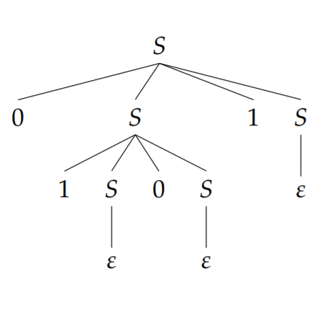
Consider CFG from the previous lecture: \[ S\to 0\, S\, 1\, S\, |\, 1\, S\, 0\, S\, |\, \varepsilon \] and \[ L(G) = \left\{ w\in \Sigma^*: | w | _ 0 = | w | _1 \right\} \]

Here is an example of a derivation of string 0101:

S ⇒ 0 S 1 S ⇒ 0 1 S 0 S 1 S ⇒ 0 1 0 S 1 S ⇒ 0 1 0 1 S ⇒ 0 1 0 1

This is an example of a left-most derivation, which means that it is always the leftmost variable that gets replaced at each step.

Every string that can be generated by a particular context-free grammar can also be generated by that same grammar using a left-most derivation.

Parse trees

With any derivation of a string by a context-free grammar we may associate a tree, called a parse tree, according to the following rules:

• node: var/symbol/\(\varepsilon \), root: start var.
• each node corresponding to a symbol or \(\varepsilon \) is a leaf node; each node corresponding to a var has one child for each symbol or variable with which it is replaced. The children of each (variable) node are ordered in the same way as the symbols and variables in the rule used to replace that variable.

The previous derivation yields this parse tree:

Ambiguity

Sometimes a context-free grammar will allow multiple parse trees (or, equivalently, multiple left-most derivations) for some strings in the language that it generates.

Here is a different derivation of string 0101:

S ⇒ 0 S 1 S ⇒ 0 1 S ⇒ 0 1 0 S 1 S ⇒ 0 1 0 1 S ⇒ 0 1 0 1.

corresponds to this parse tree:

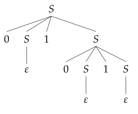
For a given CFG \(G \), there exists at least one string \(w\in L(G) \) having at least two different parse trees, then the CFG \(G \) is said to be ambiguous.

Designing unambiguous CFGs

For example, we can come up with a different context-free grammar for the language (previous example: same number of 1s and 0s).

S → 0 X 1 S | 1 Y 0 S | ε
X → 0 X 1 X | ε
Y → 1 Y 0 Y | ε

Here is another example of how an ambiguous CFG can be modified to make it unambiguous. Let us define an alphabet \(\Sigma = \left\{ a,b,+,*,(,) \right\} \) along with a CFG, ambiguous:

S → S + S | S ∗ S | ( S ) | a | b

We can, however, come up with a new CFG for the same language that is much better—it is unambiguous and it properly captures the meaning of arithmetic expressions. Here it is:

S → T | S + T
T → F | T ∗ F
F → I | ( S )
I → a | b

Variables T generate terms, the variable F generates factors, and the variable I generates identifiers. An expression is either a term or a sum of terms, a term is either a factor or a product of factors, and a factor is either an identifier or an entire expression inside of parentheses.

Inherently ambiguous languages

There are some context-free languages that can only be generated by ambiguous CFGs. Such languages are called inherently ambiguous context-free languages. An example of an inherently ambiguous context-free language is this one: \[ \left\{ 0^n1^m2^k:n=m \text{ or }m=k \right\}. \] Intuition: 0ⁿ1ⁿ2ⁿ will always have multiple parse trees for some sufficiently large natural number n.

Chomsky normal form

To be more precise about the specific sort of CFGs and parse trees we’re talking about, it is appropriate at this point to define what is called the Chomsky normal form for context-free grammars.

Definition 8.1

A CFG \(G \) is in Chomsky normal form if every rule of \(G \) has one of the following three forms:

1. X → YZ, for variables X, Y, and Z, and where neither Y nor Z is the start variable,
2. X → σ, for a variable X and a symbol σ, or
3. S → ε, for S the start variable.

Theorem 8.2

Let Σ be an alphabet and let A ⊆ Σ^* be a context-free language. There exists a CFG G in Chomsky normal form such that A = L(G).

The usual way to prove this theorem is through a construction that converts an arbitrary CFG G into a CFG H in Chomsky normal form for which it holds that L(H) = L(G).

Finally, it must be stressed that the Chomsky normal form says nothing about ambiguity in general—a CFG in Chomsky normal form may or may not be ambiguous, just like we have for arbitrary CFGs. On the other hand, if you start with an unambiguous CFG and perform the conversion described above, the resulting CFG in Chomsky normal form will still be unambiguous

Lec 9

Closure under the regular operations

Theorem 9.1

A, B context-free. Then \(A\cup B, AB, A^* \) are context-free.

Proof. Construct \(G \).

Every regular language is context-free

Two ways to prove.

Theorem 9.2

A regular language, then A is context-free.

First proof. Associate a CFG \(G \) by recursively applying simple constructions. Discuss by cases: 6 cases.

Second proof. DFA.

Intersections of regular and context-free languages

Theorem 9.3

A context-free, B regular. \(A\cap B \) context-free.

Proof. The main idea of the proof is to define a new CFG H such that L(H) = A ∩ B

Prefixes, suffixes, and substrings

If A is context free, then Prefix(A), Suffix(A), Substring(A) are all context-free.

Construct CFGs for each.

Lec 10

Pumping lemma for CFL

If you have a parse tree for the derivation of a particular string by some context-free grammar, and the parse tree is sufficiently deep, then there must be a variable that appears multiple times on some path from the root to a leaf.

Lemma 10.1

(Pumping lemma for context-free languages). \(A \) context-free. There exists a positive integer \(n \) (pumping length of \(A \)) that possesses the following property. For every string \(w\in A \) with \(| w |\ge n \), it is possible to write \(w=uvxyz \) for some choise of strings \(u,v,x,y,z\in \Sigma^* \) such that

1. \(vy\ne \varepsilon \)
2. \(| vxy |\le n \), and
3. \(u v^i x y^i z\in A \) for all \(i\in \mathbb N \).

Use this lemma

\(A= \left\{ 0^m 1^m 2^m: m\in \mathbb N \right\} \) is not context-free.

\(B = \{ 0^m: m \) is a perfect square \(\} \) is not context-free.

Every context-free language over a single-symbol alphabet must be regular. (Proof skipped)

Σ = {0, 1, #}. \(C= \{ r \# s: r,s\in \left\{ 0,1 \right\}^*, \) r is a substring of s \(\} \) is not context-free.

Discuss by cases: # in u, v, x, y, z.

Closure properties

A, B CFL \(\not\implies A\cap B, \bar A \) are context-free.

Lec 11

Pushdown automata

The pushdown automaton (or PDA) model of computation is essentially what you get if you equip NFAs each with a single stack. A transition labeled by

• an input symbol or ε: read a symbol or take an ε-transition
• (↓, a): push symbol a onto the stack
• (↑, a): pop the symbol a off of the stack.

Definition 11.1

PDF is 6-tuple \(P=(Q,\Sigma, \Gamma, \delta, q_0, F) \). Q finite nonempty set of states. Σ is an alphabet (called the input alphabet). Γ is an alphabet (called the stack alphabet), δ is a function. F is a set of accept states.

It is required \(\Sigma \cap \operatorname{Stack}(\Gamma) = \varnothing \) where \(\operatorname{Stack}(\Gamma) = \left\{ \downarrow, \uparrow \right\}\times \Gamma \).

Assume we read it from left to right and imagine that we started with an empty stack. If a string does represent a valid sequence of stack operations, we will say that it is a valid stack string; and if a string fails to represent a valid sequence of stack operations, we will say that it is an invalid stack string.

Definition 11.2

Let P be a PDA, w be a string. P accepts w if there exists \(m\in \mathbb N \), a sequence of states \(r _ 0,\ldots, r _ m \), and a sequence \(a _ 1,\ldots, a _ m\in \Sigma \cup \operatorname{Stack}(\Gamma) \cup \left\{ \varepsilon \right\} \). Then 4 properties to hold.

Shorthand notation: \(\sigma \uparrow a \downarrow b \) means σ is read, a is popped, b is pushed.

A CFL. B finite language. Then \(A\triangle B \) is context-free.

Let Σ and Γ be disjoint alphabets, let A ⊆ (Σ ∪ Γ)^∗ be a context-free language, and define \(B= \{ w\in \Sigma^*: \) there exists a string x ∈ A such that w is obtained from x by deleting all symbols in Γ \(\} \) is context-free.

Equivalence of PDAs and CFGs

Every context-free language is recognized by a PDA. Every language recognized by a PDA is context-free

Lec 12

Church–Turing thesis: Any function that can be computed by a mechanical process can be computed by a Turing machine

Turing machine components and definitions

Three components of a TM:

1. The finite state control.
2. The tape head.
3. The tape.

Definition 12.1

deterministic Turing machine (or DTM, for short) is a 7-tuple \[ M=(Q, \Sigma, \Gamma, \delta, q _ 0, q _ {acc}, q _ {rej}), \] Q finite nonempty set of states; \(\Sigma \) input alphabet, may not include blank symbol \(\sqcup \); \(\Gamma \) tape alphabet, must satisfy \(\Sigma \cup \left\{ \sqcup \right\} \subseteq \Gamma \); \(\delta\) transition function; q0 initial state, q_acc, q_rej accept reject state.

Turing machine computations

Three possible alternatives for a DTM M on a given input string w:

1. M accepts w.
2. M rejects w.
3. M runs forever on input w.

When we speak of a configuration of a DTM, we are speaking of a description of all of the Turing machine’s components at some instant:

1. the state of the finite state control,
2. the contents of the entire tape, and
3. the tape head position on the tape.

We express a config in the form \[ u(q,a)v \] u has no blank on the left, v has no blank on the right. This config means: state of M is q; tape head of M is positioned over symbol a that occurs between u and v.

We define a function \(\gamma \): \[ \gamma(u(q,a)v) = \alpha (u)(q,a)\beta(v) \] just throws away all blank symbols on the left-most end of u and the right-most end of v.

Definition 12.2

yields relation \(\vdash_M \) on pairs of expressions representing configs:

1. \(\delta(p,a)=(q,b,\to) \): \[ u(p, a) c v \vdash _ {M} \gamma(u b(q, c) v) \qquad u(p, a) \vdash _ {M} \gamma(u b(q, \sqcup)) \]
2. \(\delta(p,a)=(q,b,\gets) \): \[ u c(p, a) v \vdash _ {M} \gamma(u(q, c) b v) \qquad (p, a) v \vdash _ {M} \gamma((q, \sqcup) b v) \]

Also, we have \(\vdash _ M^* \) to denote the reflexive, transitive closure of \(\vdash_M \).

Definition 12.3

M accepts, rejects w. M runs forever on input w.

Definition 12.4

Let A be a language.

1. A is Turing recognizable if there exists a DTM M s.t. \(A=L(M) \).
2. The language A is decidable if there exists a DTM M that satisfies two conditions:
   • \(A=L(M) \), and
   • M never runs forever (either accept or reject).

A simple example of a Turing machine

Check section 12.3 for an example of a Turing machine, which describes the language \(A=\left\{ 0^n 1^n \, : \, n\in \mathbb N \right\} \).

Lec 13

Variants of Turing machine

DTMs allowing stationary tape heads: add \(\downarrow \) to \(\left\{ \gets, \to \right\} \).

DTMs with multi-track tapes: Specifically, we may suppose that the tape has k tracks for some positive integer k, and for each tape head position the tape has k separate tape squares that can each store a symbol.

DTMs with one-way infinite tapes:

• It is easy to simulate a DTM with a one-way infinite tape using an ordinary DTM (with a two-way infinite tape). For instance, we could drop a special symbol, such as ✂, on the two-way infinite tape at the beginning of the computation, to the left of the input. If the tape head ever scans the special ✂ symbol during the computation, it moves one square right without changing state.
• Simulation of a two-way infinite tape with a one-way infinite tape, two ways: two tracks, A special tape symbol, such as ➥, could be placed on the first square of the bottom track to assist in the simulation; A special symbol could be placed in the left-most square of the one-way infinite tape, and anytime this symbol is scanned the DTM can transition into a subroutine in which every other symbol on the tape is shifted one square to the right in order to “make room” for a new square to the left.

Multi-tape DTMs: A multi-tape DTM works in a similar way to an ordinary, single-tape DTM, except that it has k tape heads that operate independently on k tapes.

Encoding various objects as strings

Encoding strings over one alphabet by strings over another: be aware of ambiguity. For example,

0 -> 1     1 -> 10     2 -> 100     3 -> 1000

Encoding multiple strings into one: introduce the symbol # to indicate separation between the strings.

Numbers, vectors, and matrices

Encoding graphs as binary strings: encode adjacency matrix, or a list of edges.

Lec 14

Encoding for different models of computation

We want to encode things over the alphabet \(\Sigma \). Encode DFAs, say DFA \(D= (Q,\Gamma, \delta, q _ 0 , F) \):

1. Denote the result (binary string) by \(\langle D \rangle \).
2. Only assumption: Q is finite and nonempty.
3. \(\Gamma \) could be different from \(\Sigma \). We could just assume \(\Gamma= \left\{ 0,\ldots,m-1 \right\} \).

Encode over {0, 1, #, /} first. A hypothetical example: \[ \underbrace{1011} _ {m} \# \underbrace{01100 \cdots 011} _ {F} \# \underbrace{0 / 0 / 110 \# 0 / 1 / 1001 \# \cdots \# 11001 / 1010 / 011} _ {\delta} \] a/b/c (a,b,c are natural numbers): \(\delta(q _ a,b)=q _ c \)

Encoding NFA, CFG, DTM is similar.

Simple examples of decidable languages

We denote the encoded string by \(\langle X,Y,\ldots, Z\rangle \). Consider the following language: A = { \(\langle n, m\rangle \) : n and m are natural numbers that satisfy n > m }. The problem is decidable for any reasonable encoding scheme whatsoever. We can do two-tape DTM that decides A.

One can imagine many other languages based on the natural numbers, arithmetic, and so on. These examples below are decidable:

C = {<a,b,c> : a,b,c natural num, a+b=c},
D = {<a,b,c> : a,b,c natural, ab=c},
E = {<n> : n prime}

We describe DTM in a high level. Take language E for an example:

On input \(n \), where n is a natural number:

1. If \(n\le 1 \), reject.
2. \(t\gets 2 \).
3. If t = n, accept.
4. If t divides n evenly, then reject.
5. \(t\gets t+1 \) and goto step 3.

Note that first line implicitly rejects all invalid inputs.

Here is one final example of a simple decidable language, which this time concerns graph reachability. R = { \(\langle G, u, v\rangle \) : there exists a path from u to v in G }. (G undirected)

On input \(\langle G, u, v\rangle \), where G is an undirected graph and u and v are vertices of G:

1. \(S\gets \left\{ u \right\} \)
2. \(F \gets 1 \)
3. For each vertex w of G, do:
4.      If w is not contained in S and w is adjacent to a vertex in S, then set S ← S ∪ {w} and F ← 0.
5. If F = 0 then go to 2.
6. Accept if \(v\in S \), otherwise reject.

Languages concerning DFAs, NFAs, and CFGs

\[ A _ {DFA} = \left\{ \langle D, w \rangle \, : \, D\text{ is a DFA and }w\in L(D) \right\} \]

On input \(\langle D,w \rangle \), where D is DFA, w string:

1. If w contains symbols not in alphabet of D, reject.
2. Simulate the computation of D on input w. If this simulation ends on an accept state of D, then accept, and otherwise reject.

Similarly, for NFA, because it really isn’t clear how one simulates a nondeterministic computation with a DTM. We can convert NFA to DFA first, then do the same thing. Similar for regular expressions.

A different example: \[ E _ {DFA} = \left\{ \langle D \rangle\,:\, \text{D is DFA and }L(D)=\varnothing \right\} \]

The approach is similar to the graph reachability example from before: see if there is an accept state that is reachable from the start state.

One more example: \[ EQ _ {DFA}= \left\{ \langle D,E \rangle \,:\, L(D)=L(E) \right\} \]

On input \(\langle D,E \rangle \), D,E are DFAs:

1. Construct a DFA M for which it holds that L(M) = L(D) \(\triangle \) L(E).
2. If \(\langle M \rangle \in E _ {DFA} \), then acept, otherwise reject.

Now let’s consider \(A _ {CFG} \).

On input \(\langle G,w \rangle \), where G is a CFG and w is a string:

1. Convert G into an equivalent CFG H in Chomsky normal form.
2. If w = ε then accept if S → ε is a rule in H and reject otherwise.
3. Search over all possible derivations by H having 2|w| − 1 steps (of which there are finitely many). Accept if a valid derivation of w is found, and reject otherwise.

Finally, the language E_CFG can be decided using a variation on the reachability technique. In essence, we keep track of a set containing variables that generate at least one string, and then test to see if the start variable is contained in this set.

EQ_CFG is not decidable. Some other examples of undecidable languages concerning context-free grammars are as follows: the string is \(\langle G \rangle \), and conditions are

• G is a CFG that generates all strings over its alphabet
• G is an ambiguous CFG
• G is a CFG and L(G) is inherently ambiguous

Lec 15

Simulating one Turing machine with another

\[ A _ {DTM} = \left\{ \left\langle M,w \right\rangle: M \text{ is a DTM and }w \in L(M) \right\} \]

Consider the language A_DTM. Not decidable, but Turing recognizable. In particular we can define a DTM \(U \) (universal Turing machine) having the following high-level description:

On input \(\langle M,w \rangle \), where M is a DTM and w is a string:

1. If w is not a string over the alphabet of M, then reject.
2. Simulate M on input w. If at any point in the simulation M accepts w, then accept; and if M rejects w, then reject.

If you have a description of a DTM M and an input string w, you can simulate M on input w by keeping track of the configuration of M and repeatedly update it one step at a time. For the DTM U as defined above, it holds that L(U) = A_DTM, and therefore ADTM is Turing recognizable. On the other hand, U does not decide A_DTM because it might run forever on some inputs.

If we included a limitation on the number of steps a DTM is allowed to run, as part of the input, we obtain a variant of the language defined above that is decidable: S_DTM = {\( \langle M,w,t \rangle \) : M DTM, w string, t natural num, M accepts w within t steps }.

This language could be decided by a DTM similar to U defined above, but where it cuts the simulation off after t steps if M has not accepted w.

A non-Turing-recognizable language

Define a language \[ \text{DIAG} = \left\{ \left\langle M \right\rangle : M \text{ is a DTM and } \left\langle M \right\rangle \notin L(M) \right\} \]

Over a fixed alphabet (such as the binary alphabet). The language DIAG contains all strings that, with respect to the chosen encoding scheme, encode a DTM that does not accept this encoding of itself.

Theorem 15.1

The language DIAG is not Turing recognizable.

Some undecidable languages

Proposition 15.3

The language A_DTM is undecidable.

Famous relative \[ \text{HALT} = \left\{ \left\langle M,w \right\rangle : M\text{ is a DTM that halts on input }w \right\} \]

Let us agree that the statement “M halts on input w” is false in case w contains symbols not in the input alphabet of M – purely as a matter of terminology.

Easy to see HALT is Turing recognizable.

Proposition 15.4

The language HALT is undecidable.

A couple of basic Turing machine tricks

Limiting infinite search spaces

Proposition 15.5

A, B Turing recognizable. \(A\cup B \) is Turing recognizable.

Proof. Define a new DTM M as follows:

On input w:

1. \(t\gets 1 \)
2. Run M_A for t steps on w. If M_A has accepted within t steps, then accept.
3. Run M_B for t steps on w. If M_B has accepted within t steps, then accept.
4. \(t\gets t+1 \), and goto 2.

Using t to bound the number of steps of both simulations is an effective way to handle this situation.

Theorem 15.7

\(A, \bar A \) are Turing recognizable. The language A is decidable.

Hard-coding input strings

DTM \(M \), string \(x \). Define \(M _ x \) as follows:

On input \(w \): Ignore the input string \(w \) and run \(M \) on input \(x \).

\[ E _ {DTM} = \left\{ \left\langle M \right\rangle : M \text{ is a DTM with }L(M) = \varnothing \right\} \]

Proposition 15.8

E_DTM is not decidable.

Proof. Assume decidable. T decides this language. Define a new DTM \(K \):

On input \(\left\langle M,w \right\rangle \):

1. If w is not a string over input alphabet of M, reject.
2. Compute an encoding \(\left\langle M _ w \right\rangle \).
3. Run T on input \(\left\langle M _ w \right\rangle \). If T accepts \(\left\langle M _ w \right\rangle \), then reject, ow accept.

M DTM, w ∈ L(M). Consider K on input \(\left\langle M,w \right\rangle \). \(M _ w \) accepts every string, then \(L(M _ w)\ne \varnothing \), then T rejects \(\left\langle M _ w \right\rangle \)。

On the other hand w ∉ L(M). Similar argument, K reject \(\left\langle M _ w \right\rangle \).

Thus K decides A_DTM.

Lec 16

Computable functions and reductions

Definition 16.1

\(f : \Sigma ^ * \to \Sigma ^ * \) a function. f is computable if there exists a DTM M whose yields relations satisfies \[ ( q _ 0, \sqcup) w \vdash _ M ^* (q _ {acc}, \sqcup) f(w) \] for every string \(w \in \Sigma^* \).

So if we run M on w, it will accept, with just the output \(f(w) \) written on the tape.

The specific type of reduction we will consider is sometimes called a mapping reduction — but because this is the only type of reduction we will be concerned with, we’ll stick with the simpler term reduction.

Definition 16.2

A, B be languages. A reduces to B if there exists a computable function f such that \(w\in A \iff f(w)\in B \) for all w. One writes \(A \le _ m B \) to denote A reduces B. Any such function f is called a reduction from A to B.

Theorem 16.3

A, B be languages. \(A \le _ m B \).

1. B decidable, then A decidable.
2. B Turing recognizable, then A Turing recognizable.

Proposition 16.4

\(\le _ m \) is transitive.

Proposition 16.5

\(A \le _ m B \iff \bar A \le _ m \bar B \)

Proving undecidability through reductions

When we prove a reduction on an assignment or exam, we would not be expected to provide this much detail.

Example 16.6

A_DTM ⩽_m HALT

Example 16.7

DIAG ⩽_m E_DTM

Example 16.8

A_DTM ⩽_m AE where AE = { \(\left\langle M \right\rangle \) : M is a DTM that accepts \(\varepsilon \)}.

Example 16.9

E_DTM ⩽_m REG where REG = { \(\left\langle M \right\rangle \) : M is a DTM such that L(M) is regular }

Lec 17

Decidable language closure properties

Proposition 17.1 & 2

A, B decidable languages. Then \(A\cup B, AB, A^*,\bar A \) are decidable.

Example 17.3

Prefix(A) might not be decidable, even if A is decidable.

Turing-recognizable language closure properties

Proposition 17.4 & 5

A, B Turing-recognizable. Then \(A\cup B, AB, A^*, A\cap B \) are Turing recognizable.

Nondeterministic Turing machines

Definition 17.6

A NTM is a 7-tuple \[ N = (Q, \Sigma, \Gamma, \delta, q _ 0, q _ {acc}, q _ {rej}), \] where Q is finite & nonempty set of states; the other terms are similar as NFA + DTM.

When we think about the yields relation of an NTM N, and the way that it computes on a given input string w, it is natural to envision a computation tree. Note that we allow multiple nodes in the tree to represent the same configuration, as there could be different computation paths (or paths starting from the root node and going down the tree) that reach a particular configuration.

Theorem 17.7

There exists an NTM N such that L(N) = A iff A is Turing recognizable.

The range of a computable function

Theorem 17.8

A be a nonempty language. The following two statements are equivalent:

1. A is Turing recognizable.
2. There exists a computable function f such that \(A = \operatorname{range} (f) \)

Corollary 17.10

A be any infinite Turing recognizable language. Then there exists an infinite decidable language \(B \subseteq A \).

Lec 18

Time complexity

We will start with a definition of the running time of a DTM, assuming that this DTM never runs forever.

Definition 18.1

Let \(M \) be a DTM with input alphabet \(\Sigma \) that halts on every input string \(w\in \Sigma^ *. \) The running time of M is the function \(t \) defined as follows for each \(n\in \mathbb N \): \[ t(n) = \text{max # of steps required for M to halt, over all w, with } | w | = n. \]

Definition 18.2

Let \(f: \mathbb N \to \mathbb N \) be a function. A language \(A \) is contained in the class \(\mbox{DTIME}(f) \) if there exists a M decides A and whose running time t satisfies \(t(n) = O(f(n)) \).

Theorem 18.4

\(A \) a language. If there exists a DTM \(M \) that decides \(A \) in time \(o(n\log n) \), meaning that the running time \(t \) of \(M \) satisfies \[ \lim _ {n\to\infty} \frac{t(n)}{n\log n}=0, \] then \(A \) is regular.

Definition 18.5

Let \(f \) be a function satisfying \(f(n) = \Omega (n\log n) \). The function f is time constructible if there exists a DTM M that operates as follows:

1. On each input \(0^n \) M computes the binary representation of \(f(n) \), for every natural number n.
2. M runs in time \(O(f(n)) \).

These are functions that can serve as upper bounds for DTM computations.

Time-hierarchy theorem

A highly informal statement of the theorem is this: more languages can be decided with more time.

用不大正式的说法解释，这理论告诉我们图灵机在给予更多时间之后，保证能解决更多的问题。

from wiki.

Theorem 18.6

(Time-hierarchy theorem) For time-constructible function f, \[ {\mathsf {DTIME}}\left(o\left({\frac {f(n)}{\log f(n)}}\right)\right)\subsetneq {\mathsf {DTIME}}(f(n)) \]

Corollary 18.7

For all positive integer k, \[ {\mathsf {DTIME}}(n^k) \subsetneq {\mathsf {DTIME}}(n^ { k+1}) \]

Polynomial and exponential time

We define two complexity classes: \[ \mathrm{P}=\bigcup _ {k \geq 1} \operatorname{DTIME}\left(n^{k}\right) \quad \text { and } \quad \mathrm{EXP}=\bigcup _ {k \geq 1} \mathrm{DTIME}\left(2^{n^{k}}\right) . \]

Lec 19

The complexity class NP

There are two, equivalent ways to define the complexity class NP that we will cover in this lecture.

NP as certificate verification

Definition 19.1

A is contained in NP if exist positive int k, a time-constructible function \(f(n)=O(n^k) \), and a language \(B\in {\rm P} \) such that \[ A = \left\{ x\in \Gamma^* \mid \exists y\in \Sigma^* \text{ s.t. } | y | = f(| x |) \text{ and } \left\langle x,y \right\rangle \in B \right\} \]

The essential idea that A is efficiently verifiable.

NP as polynomial-time nondeterministic computations

We define NTIME(f): the class of all languages that are decided by a nondeterministic Turing machine running in time \(O(f(n)) \).

We define NP \[ {\rm NP} = \bigcup _ {k\ge 1} {\rm NTIME} (n^k) \]

NP is short for nondeterministic polynomial time.

Observe that \({\rm P \subseteq NP \subseteq EXP} \)

Polynomial-time reductions and NP-completeness

Definition 19.4

A, B be languages. A polynomial-time reduces to B if there exists a polynomial-time computable function \(f \) such that \[ w\in A \iff f(w)\in B \] for all \(w \). One writes \[ A \le _ m^p B \]

Definition 19.5

B a language.

1. B is NP-hard, if for every \(A\in {\rm NP} \), \(A\le_ m^p B \).
2. B is NP-complete, if B is NP-hard and \(B\in {\rm NP} \).

Assume A, B, C languages.

1. \(\le _ m^p \) is transitive.
2. \(A \le _ m^p B \), and \(B\in P \), then \(A\in P \).
3. \(A \le _ m^p B \), and \(B\in NP \), then \(A\in NP \).
4. A is NP-hard, \(A \le _ m^p B \), then B is NP-hard.
5. A is NP-complete, \(B\in NP, A\le _ m^p B \), then B is NP-compelte.
6. If A is NP-hard and A ∈ P, then P = NP.

Lec 20

Boolean circuits

Definition 20.1

An n-input, m-output Boolean circuit C is a directed acyclic graph, along with various labels associated with its nodes, satisfying the following constraints:

1. The nodes of C are partitioned into three disjoint sets: the set of input nodes, the set of constant nodes, and the set of gate nodes.
2. The set of input nodes has precisely n members, labeled \(X _ 1,\ldots, X _ n \). Each input node and must have in-degree 0.
3. Each constant node must have in-degree 0, and must be labeled either 0 or 1.
4. Each gate node of C is labeled by an element of the set {∧, ∨, ¬}.
5. Finally, m nodes of C are identified as output nodes, and are labeled \(Y _ 1,\ldots, Y _ m \). An output node can be an input node, a constant node, or a gate node.

Universality of Boolean circuits

Every Boolean function of the form \(f: \left\{ 0,1 \right\}^n \to \left\{ 0,1 \right\}^m \), for positive integers n and m, can computed by some Boolean circuit C.

Boolean circuits and Turing machines

Theorem 20.2

Let f be a time-constructible function, and let M be a DTM with binary input alphabet whose running time t(n) satisfies \(t(n) \le f(n) \) for all natural number n. There exists a family \[ \mathcal F = \left\{ C _ n : n \in \mathbb N \right\} \] of Boolean circuits, where each circuit C_n has n inputs and 1 output, such that the following two properties are satisfied:

1. For every natural number n and every x ∈ {0, 1}ⁿ, M accepts x iff C_n(x) = 1
2. size(C_n) = O(f(n)²)

Lec 21

Circuit satisfiability

Define a language \[ \mbox{CIRCUIT-SAT} = \left\{ \left\langle C \right\rangle : C \text{ is an $m$-input, 1-output, and satisfiable} \right\} \]

Easy to see CIRCUIT-SAT ∈ NP.

Theorem 21.1

(Cook–Levin theorem, part 1). CIRCUIT-SAT is NP-complete.

Proof. It remains to prove that CIRCUIT-SAT is NP-hard. Then let \(A\subseteq \Gamma^* \) be any language in NP. We then prove \(A \le _ m ^ p \mbox{CIRCUIT-SAT} \).

Satisfiability of 3CNF formulas

A Boolean formula \(\phi \) in Boolean variables \(X _ 1,\ldots, X _ n \) is said to be CNF if \[ \phi = \psi _ 1 \wedge \cdots \wedge \psi _ m \] where each \(\psi _ k \) is an OR of a collection of variables or their negations.

A formula is said to be a 3CNF formula if it is the case that it is a CNF form exactly three literals in each clause. Let us define a new language: \[ \mbox{3SAT} = \left\{ \left\langle \phi \right\rangle : \phi \text{ is a satisfiable 3CNF formula} \right\} \]

Theorem 21.2

(Cook–Levin theorem, part 2). 3SAT is NP-complete.

Proof. We just prove \(\mbox{CIRCUIT-SAT} \le _ m ^ p \mbox{3SAT} \)