SYDE 522: Machine Intelligence
Hamid R. Tizhoosh
Estimated study time: 32 minutes
Table of contents
Introduction to Artificial Intelligence
Objectives of this course:
- basic concepts of AI
- different methods for function approximation
- select the right learning scheme
- difference between shallow & deep learning
- verify the learning capability
- run and evaluate experiments
- write a scientific paper
Lecture Topics:
- Encoding/embedding: data compression, PCA, t-SNE, Fisher Vector, …, \(k \)-fold cross validation, leave-one-out
- Classification/clustering: K-means, FCM, SVM, self-organizing maps
- Learning: Perceptron, backpropagation, CNN, AEs
- Reinforcement learning: check CS 885
- Uncertain vs. vague: Probability, FuzzyLogic, DTs, RFs
Why interest in AI?
- Recent progress in algorithms
- Availability of data
- Computational power
History of AI
1901 - PCA (K. Pearson)
1933 - PCA development (H. Hotelling)
1958 - Perceptron (F. Rosenblatt)
1965 - Fuzzy Sets (L. Zadeh)
1969 - Limitation of Perceptron (Minsky/Papert)
1982 - SOM (T. Kohonen)
1986 - Backpropation (Rumelhart/Hinton)
1986 - ID3 algorithm (J.R. Quinlan)
1993 - C 4.5 algorithm (J.R. Quinlan)
1995 - SVM (Cortes/Vapnik)
1995/2001 - Random Forest (T.K.Ho/L.Breiman)
1995 - CNN (LeCunn/Bengio)
2006 - Fast learning for deep belief Nets (Hinton et al.)
2007 - Greedy layer-wise training for deep Nets (Bengio et al.)
2012 - AlexNet
Main Tasks for AI
- Classification
- Estimation/Prediction
- Search
- Optimization
- Inference
All these is approximation: you have a black box \(f(x) \), some \(x \) goes in and some \(y \) goes out. \(f \) is unknown. The simplest approach is regression.
What is intelligence?
“the act of knowing” \(\implies \) intelligence \(\stackrel{?}{=} \) knowledge
“the exercise of understanding” \(\implies \) intelligence = understanding
| humans | machines | |
|---|---|---|
| thought | reason | rational decisions |
| actions | act | rational actions (AI) |
Can we measure intelligence?
Philosophical Foundations and Dimensionality Reduction
Check this paper
Can machine think?
Alan Turing assumed we can build intelligent machines. Measuring intelligence is what he is proposing.
Turing anticipated all AI fields:
- searching. Not like browsing, and you type sth in search engine. We are talking about explicit ones: whenever you see sb and remember the face, that is a search. The challenge is the visual info is stored in a highly complicated way, and search mechanism is very sophisticated.
- reasoning. That’s where we failed Turing test. We cannot search intelligently, and we cannot reason based on the knowledge you acquired.
- knowledge representation
- NLP
- computer vision
- learning
The Chinese Room
J. R. Searle
In the room, the person is non-Chinese. Two books inside: rule and dictionary. From outside, people come, put in Chinese text, and come out (flawless) English text.
Can this person understand Chinese? Can the room understand Chinese?
Let’s look at an example.
Tic-Tac-Toe
Version 1: Look-Up Table [Answer for each situation is hard-coded]
Version 2:
- A: Attempt to place two marks in row
- B: If opponent has two marks in a row, then place a mark in the third position.
Version 3: Represent the state(understanding) of the game
- Current board position?
- next legal moves?
Use an evaluation function.
- Rate the next move! (how likely to win?)
- Look-ahead of possible opponent’s move!
<-----Stupid ----------------------- intelligent----->
Version 1                   2                         3
AI = Function Approximation
We need “data” for any approximation. For example, linear regression.
AI = Operation intelligently on data to extract the relationship between in- and outputs.
- Training data for learning.
- testing data for validation.
Problems
- Not enough data \(\to \) Augmentation
- Too much data \(\to \) Dimensionality reduction
Desired
- no correlation
- high variance
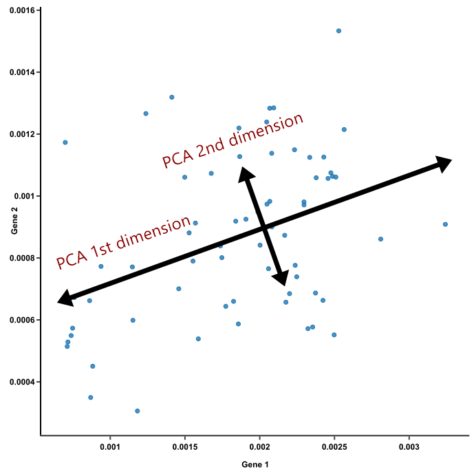
PCA
\(x' \) passes through the “mean” and delivers max variance when samples are projected into it. Process is repeated until we find \(n \) such axes \(\langle x_1,x_2,\ldots,x_n\rangle \). intelligent: \(x\in \mathbb R^d \implies n \ll d \).
Principal Component Analysis (PCA) is the algorithm to find orthogonal axes that diagonalize the covariance matrix. What does this mean?
First let’s get used to some notations…
- \(x \): scalar.
- \(\boldsymbol x \): vector.
- \(X \): set.
- \(\boldsymbol X \): matrix.
Covariance matrix
\[ \Sigma = \operatorname{cov}(\underbrace{x_i} _ {i\text{-th input}}, \underbrace{x_j} _ {j\text{-th input}}) = \mathbb E \left[ (x_ i - \mu _ i) (x _ j - \mu _ j) \right] \]where \(\mu _ i = \mathbb E[ x _ i], \mu _ j = \mathbb E[ x _ j] \).
Are \(x_i \) and \(x_j \) changing together? (correlated)
Generalization of Covariance: \(\Sigma = E[(\boldsymbol x - E[\boldsymbol x]) (\boldsymbol x - E[\boldsymbol x])^T ] \)
Principal Component Analysis
PCA
main features selection. Which components (=features) are important to keep?
- Significance = variance.
- Intelligence = recognizing the significance
Staring point is a file with a table: where the columns: \(x_ 1, x_ 2,\ldots \) are features and rows: (1, 2, 3, …) are observations.
Covariance matrix \(C = E[ x x^T] \)
Diagonalizing \(C \) using a suitable orthogonal transformation matrix \(A \) by obtaining \(N \) orthogonal “special vectors” \(u_ i \) with “special parameters” \(\lambda _ i \)
Principal components: \(\lambda_ 1 \) most important, \(\lambda _ N \) least important. Pick \(N' \ll N \), so-called dimensionality reduction.
PCA is
- a linear transformation
- unsupervised
- uses statistics and calculus
- dimensionality reduction algorithm
- a visualization algorithm
- intelligent because it recognizes significance
AI & Data
Data types: numbers/symbols/text/images/videos/audio files…
Pre-processing: filtering/normalization/outlier detection/dimensionality reduction/augmentation/…
Data representation:
- Hand-crafted features (e.g., stats, SIFT)
- automatic feature extraction (e.g. deep features)
Encoding: (compression/embedding)
- no learning
- PCA
- Fisher Vector
- LDA
- VLAD (vector of locally aggregated descriptors)
- …
- with learning
- Auto-Encoders. ML DDoS Detection :)
- t-SNE
Applications of PCA
- Data reduction
- Data visualization
- Data classification
- Factor analysis
- Trend analysis
- Noise removal
A meaningful chain:
You will see that this is not always desirable.
Project
(not sure if this helps…)
- Find a problem
- Analyze the problem (input/output/knowledge)
- Select approach (architecture, parameters, …)
- Design the approach
- Training
- Re-train if necessary
- Recall phrase (unseen data)
- Compare against other methods
Linear Discriminant Analysis and t-SNE
LDA
linear discriminant analysis (operates of feature subspace, linear method, supervised)
- Data \(\langle x _ 1,\ldots,x _ n \rangle \)
- \(N _ 1 (N _ 2) \) samples belonging to class \(C_1 (C _ 2) \)
- Find a line that maximizes the class separation
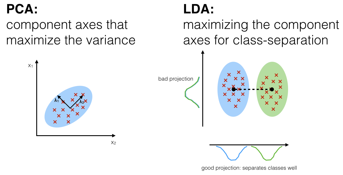
- Define a good separation measure
- Mean vector
- Driving force for separation: \(\operatorname{argmax}_ w |\tilde \mu _ 1 - \tilde \mu _ 2 | \)
- But we are ignoring the variability inside classes
Fisher’s Approach: Normalize the distance (difference) between the means by intra-class scatter.
scatter = variance: \(\tilde s _ i ^ 2 = \sum _ {y\in C _ i} (y - \tilde \mu _ i)^2 \)
intra-class scatter \(\tilde s _ 1^2 + \tilde s _ 2^2 \)
Fisher Linear Discriminant: \(\dfrac {| \tilde \mu _ 1-\tilde\mu _ 2 |^2} {\tilde s _ 1^2 + \tilde s _ 2^2} \). To be maximized!
t-SNE
t-Distributed stochastic neighbor embeddings.
- non-linear data visualizer
- t-test. t-distribution (normal distribution)
t-SNE does not use any norm (=distance metric). It uses Kullback-Leibler Divergence. Given two probability distributions \(p,q \), the KL divergence measures the distance
\[ D(p\|q)= \sum _ {x\in X} p(x)\log {p(x)\over q(x)} \]However, \(D (p \| q) \ne D(q \| p) \). Therefore, KL divergence is not a metric!
Relation to entropy \(H(X) \).
\[ H(X)=\sum _ {x\in X}p(x)\log {1\over p(x)} = \log N - D(\underbrace{p(x)} _ {\text{true dist'n}} \| p _ U(x)) \]where \(U \): uniform.
The Shannon entropy is the number of bits necessary to identify \(X \) from \(N \) equally likely possibilities, less the KL divergence of the uniform distribution from the true distribution.
t-SNE idea: hyper-dimensions \(\to \) two dimensions. Similarity in high dimensions corresponds to short distance in low dimensions.
Challenge: perplexing!
t-SNE minimizes the sum of KL divergences over all data points using a gradient descent method.
\[ Objective = \sum _ i D(P _ i \| Q _ i) = \sum _ i \sum _ j p _ {j | i} \log { p _ {j | i}\over q _ {j | i}} \]Feature Encoding: Fisher Vectors and VLAD
We’ll start by saying: AI is vision! Intelligence is to recognize people/scenes/objects/patters/…
- Face recognition
- object recognition
- Auto-captioning of images
- robot navigation
- …
Given a digital image, two possible ways for recognition:
- AI approach: given an image, then pass to some sort of AI black box, then there it comes out classes/text
- CV/AI approach: given an image, then give it to whitebox (CV), which gives you some features, then goes to blackbox of AI, then classes/text
Feature Extraction:
- Keypoint-oriented (SIFT, SURF, …): Several hundreds/thousands features
- Histogram-oriented (LBP, HOG, ELF …): one histogram
Example: Harris Corner Detection
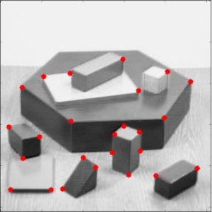
For SIFT, you get many feature vectors of length 128. Thus
\[ Image = \bigcup _ {i=1} ^ { n \text{ key points}} v _ i \]Challenge:
- Data is too large
- Data may not be descriptive
Solution: embedding/pooling/encoding
- Fisher Vectors (embedding/pooling)
- VLAD (encoding/increasing discrimination)
Fisher Vectors
We have our dataset: \(X = \left\{ x _ t | t = 1,\ldots, T \right\} \). And \(u _ \lambda \) = probability density function which models the generative process of elements of \(X \). And we have \(\lambda \in \mathbb R^M \) which are parameters of \(u_ \lambda \)
In statistics, the “score function” is the gradient (partial derivative) w.r.t. parameter \(\lambda \) of the natural log of the likelihood function. Score function \(= \nabla _ \lambda \log u_ \lambda (X) = \nabla _ \lambda \log P(x | u _ \lambda) \)
Let \(X \) be the set of D-dimensional local descriptors extracted from an image (e.g. SIFT)
\[ g _ \lambda^X = \sum _ {t=1}^T L _ \lambda \nabla _ \lambda \log u _ \lambda (x _ t) \]This is called Fisher Vector. Fisher Vector is a sum of normalized gradients statistics computed for each descriptor (= feature vector). The operation
\[ x _ t \to f _ {FK}(x _ t) = L _ \lambda \nabla _ \lambda \log u _ \lambda ( x _ t) \]is an embedding of local descriptors \(x _ t \) in a higher dimensional space which is easier for classifier.
\(L _ \lambda \): Cholesky Decomposition
\[ F _ \lambda ^{-1} = L _ \lambda ^ T L _ \lambda, \qquad K _ {FK}(X,Y) = G _ \lambda ^{X^T} F _ \lambda G _ \lambda ^{X} \]where \(K _ {FK} \) is the Fisher Kernel.
VLAD
Vector for locally aggregated descriptors
How to recognize images? Bag of Visual Words (BoVW)
Given an image \(I \), divide it into small cell/windows of size \(n \times n \) (i.e. 16x16). We vectorize visual words for convenient calculations.
Theory: you got a image, apply BoVW, and get millions of visual words, and give that to a classifier, and classifier says that’s a cat
Practice:
- too many vectors
- redundancy
- noise
General Approach: Build a codebook (dictionary) \(C = \left\{ c _ 1,\ldots,c _ n \right\} \) from \(m\gg n \) feature vectors (vectorized visual words)
Idea: Use a clustering algorithm like k-means. (\(C _ i \) is the centre of \(n \) classes found in the data.
Core Idea of VLAD: Accumulate, for each visual word \(C _ i \), the difference of the vectors \(X \) assigned to \(C _ i \), \(X - C _ i \), i.e., distribution of data w.r.t. the class centers.
\[ V _ {i,j}=\sum _ {NN(X)=C_i} X _ j - C _ {i,j} \]Here NN is the nearest neighbor. \(X _ j \) is the \(j \)-th component of descriptor. \(C _ {i,j} \) is the corresponding center
Here we do a \(L _ 2 \) normalization. \( V : = {V\over \| V\| _ 2} \)
Final Chain
Model Validation and Regularization
How to validate AI algorithms? [How do I use Turing Test in practice?]
- We get the data
- We train our algorithms:
- how do we know it has learned what is was supposed to learn?
- We should test it! If good enough, then release it! How do we make sure of this?
First factor to make sure that is good enough is to have target/objective function:
- error (minimize)
- reward (maximize)
- fitness (maximize)
- punishment (minimize)
Given the entire data \(X = \left\{ x _ t \right\} \)
Given the set of all hypotheses \(H \) (set of all possible solutions), find \(h\in H \) such that
\[ \sum _ {x _ t\in X} (x _ t^* - x _ t ^ d) = \epsilon \to 0 \]which is supervised. This constitutes a good fit for the model \(h \) into \(X \). Any concern?
Scenario #1: you have your complex data and simple solution, then you train. It does not converge. Problem is big/non-linear/non-stationary. Solution (hypothesis) is not capable of capturing the complexity.
Scenario #2: Problem is small/linear/stationary. Solution is too big such that is completely owns the problem. h is memorizing X.
What is the ultimate sign that the algorithm has really learned? It can generalize the inherent X-Y relationship to “unseen” data.
Validation = test for generalization. Idea: keep one part of data for testing. But this may not be reliable! The split may be lucky/unfortunate. So we have K-fold partition.
Random Sampling, K-fold cross validation:
But all this would work if we had a lot of data. What if we don’t? We use Leave-one-Out validation.
n-fold cross validation: vert expensive, suitable for small data.
Model complexity = \(|P | \) where \(P \) is the set of parameters of \(h\in H \). Occam’s Razor: Keep it simple! = Regularization
\[ \min \left( \underbrace{\sum _ {x _ t\in X} (x _ t^* - x _ t^d)} _ {\text{lowest error}} + \underbrace{|P |} _ {\text{smallest solution}}\right) \]Augmented error function:
\[ E' = E _ {total} + \underbrace{\lambda \cdot \text{model complexity}} _ {\substack {\text{penalized complex}\\ \text{solutions with} \\ \text{large variance}}} \]If \(\lambda \) too large, then simple models, then increase bias. Hence we use cross validation to optimize \(\lambda \).
Another model selection approach: Bayesian approach is used if we have prior knowledge.
Bayes Rule:
\[ P (model | data) = {P(data | model) \cdot P(model)\over P(data)} \]Other methods:
- Structural risk minimization
- Minimum description length
Clustering: K-means and Self-Organizing Maps
idea: Intelligence is the capability of grouping similar objects. Clustering groups “unlabeled” data into “clusters” of similar inputs.
Are clusters well-separated? Are clusters linearly separable?
Difficulties: overlaps / complicated shapes
Clustering algorithms can be divided into 2 types
- need # of clusters
- don’t need it
K-means
We start with K-means algorithm: find the centroids (prototypes)(means) of K clusters
- Randomly place K centroids
- Assign each data point to its closest cluster K
- Update the centroids
Similarity grouping happens via distance measurement. So objective (error):
\[ E = \sum _ {k=1} ^K \sum _{x\in C _ k} \|x-m _ k\| _ 2 \]where \(m _ k \) is the centroid of \(k \)-th cluster. Minimize the sum of squared errors to its prototype in each cluster.
When you do the update, centroids are the average of all \(x\in C _ k \) for \(k \in \left\{ 1,2,\ldots, K \right\} \). Stopping:
- after some iterations
- when centroids don’t change anymore
- when few/no data points change cluster
Problems of K-means:
- Needs K
- Outlier sensitive
- Hard clustering
Clustering is unsupervised learning.
SOM
Use processing units (neurons) to place centroids on an adjustable map: Self-Organizing Maps (SOM). Hypothesis: The model self-organizes based on learning rules and interactions. Processing units maintain proximity relationships as they grow. This is so-called Kohonen Map.
The input is connected with each unit (neuron) of a lattice (map).
Concept of neighborhood:
Goals:
- find weight values such that adjacent units have similar values.
- inputs are assigned to units that are similar to them
- each unit becomes the center of a cluster
Basically SOM is constrained K-means.
Given input \(X \), find the \(i \)-th unit with closest weight vector by competition. \(w _ i ^T x \) will be maximum.
For each unit \(j \) in the neighborhood \(N(i) \) of the winning neuron \(i \), we update the weights of \(j \)(\(w _ j \)
Weights outside of \(N(i) \) are not updated
SOM has 3 stages: 1. competition. 2. collaboration: concept of neighborhood. 3. Weight update.
Competition: find the most similar unit: \(i(x) = \operatorname{argmax} _ j \| x - w _ j \| _ 2 \), where \(j=1,\ldots,m; \) \(m \) = # of units.
Collaboration: Use the lateral distance \(d _ {ij} \) between the winner unit \(i \) and unit \(j \)
\[ h _ {ij} (d _ {ij}) = \exp \left(- {d _ {ij}^2\over 2\sigma^2}\right) \]Weight updates:
\[ W _ j (n+1)= W _ j(n) + \Delta W _ j \]where \(\Delta W _ j = \underbrace{\eta y_ j } _ {\text{Hebb's Rule}} - \underbrace{g(y _ j) w _ j}_{\text {Forgetting rule}} \). So complete formula for update:
\[ W _ j (n+1)= W _ j(n) + \eta (n) h _ {ij(x)}(n)[x-w _ j(n)] \]where \(\eta(n) = \eta _ 0\exp(- {n\over T _ 2}) \)
Convergence: many iterations! (e.g., several thousands times the number of units)
Stopping:
- no noticeable change
- No big change in the feature map
Problems:
- convergence may take a long time
- variable results
Support Vector Machines
Classification: Intelligence is to distinguish things.
Support Vector Machines
SVM
Assumption: classes \(\in \left\{ \oplus, \ominus \right\} \). And \(w\cdot x _ \oplus + b \ge 1, w\cdot x _ \ominus + b \le -1 \)
Also introduce a dummy variable: \(y _ i = \begin{cases} +1 & \text{for }\oplus \\ -1 & \text{for } \ominus \end{cases} \). Thus for all \(\oplus, \ominus \),
\[ y _ i (w\cdot w + b)-1\ge 0 \]Best classification: the largest margin!
\[ \begin{aligned} (x _ \oplus - x _ \ominus) \cdot {w\over \| w\|} = {(1-b)+(1+b)\over \| w\|} = {2\over \| w\|} \end{aligned} \]So we want maximize \({1\over \| w\|} \), then minimize \({\| w\|} \).
So our problem: \(\min \| w\| \quad \text{subject to }\quad y _ i(w\cdot x _ i + b)-1\ge 0 \).
Lagrange Multipliers: \(L = {1\over 2} \|w\|^2 - \sum \alpha _ i[ y _ i (w\cdot x _ i + b) - 1] \)
Derivatives are zero, then we get \(w=\sum _ i \alpha _ i y _ i x _ i \), and \(\sum \alpha _ i y _ i = 0 \). Sub \(w \) in \(L \), we get after simplification:
\[ L =\sum \alpha _ i - {1\over 2}\sum \sum \underbrace{ \alpha _ j y _ i y _ j} _ {\text{scalars}} \underbrace{x _ i \cdot x _ k} _ {\text{dot product}} \]Minimize this via quadratic optimization! Then how to classify?
\[ \sum \alpha _ i y _ i x _ i\cdot \underbrace{u} _ {\text{new data}} + b \begin{cases} \ge 0 &\implies \oplus \\ \text{otherwise} & \implies\ominus \end{cases} \]SVM only works for binary, linearly separable problems.
XOR is a non-linear problem, however, we can do transformations.
Trick! Assume \(T(x) \) is a transform that moves \(x \) to higher dimensions and making linear separation possible, then we have to calculate \(T(x _ i)\cdot T(u) \). But these would be difficult! If we had a function \(K (x_ i , x _ j)\) such that \(K (x _ i, x _ j) = T(x _ i)\cdot T( x _ j) \), then we won’t need \(T \). All we need is a “Kernel” function \(K \). We do not need \(T(x) \)! We just need to get \(T (x _ i) \cdot T(x _ j) \), and not \(T(x _ i) \) and \(T(x _ j) \) individually. This is called The Kernel Trick.
Popular kernels:
- \(K(u,v) = (u\cdot v+1)^n \)
- \(K(u,v)=\exp(-{\|u-v\|\over \sigma}) \)
Cluster Validity and Fuzzy Sets
Cluster Validity
How do we know the clusters are valid? or, at least, good enough?
Desirable:
- High inter-class separation
- High intra-class homogeneity
Define “index of validity” that uses:
- sum-of-squares within cluster (SSW) = \(\sum _ {i=1}^N \|x _ i - C _ {p _ i}\|^2 \), where we have \(N \) data points, and \(C _ {p _ i} \) is class prototype for the \(i \)-th data isntance \(x _ i \)
- sum-of-squares between clusters (SSB) = \(\sum _ {i=1}^M n _ i\|c _ i - \bar x \|^2 \), where we have \(M \) clusters, \(n _ i \) is the number of elements in cluster, \(c _ i \) is the current class mean. and \(\bar x \) is mean of means.
SSW and SSB are part of ANOVA (analysis of variance).
Other cluster validity measures:
- Calinski-Harbusz Index \(CH = \dfrac{SSB / (M-1)}{SSW/(N_M)} \)
- Hartigen Index \(H = \left(\dfrac{SSW _ M}{SSW _ {M+1}}-1\right)(N-M-1) \) or \(H = \log _ 2 \dfrac{SSB}{SSW} \)
- Dunn’s Index
where \(d (c _ i,c _ j)= \min _ {x\in c _ i,x'\in c _ j}\|x-x'\|^2 \), and \(diam(c _ k) = \max _ {x,x'\in c _ k}\|x-x'\|^2 \)
- WB Index \(WB _ M = M\cdot {SSW\over SSB} \)
We have other problems: We made a big assumption: \(x _ i\in C _ k \) and \(x _ i\notin C _ j \quad \forall j\ne k \). This is hard/dual/crisp clustering.
\[ \mu _ k (x _ i)\in \left\{ 0,1 \right\} \implies \mu _ k(x _ i)\notin [0,1] \]AI deals with imperfect info.
A bit of Set theory
\(X = \left\{ x \right\} \) universe of discourse
characteristic function of \(A: f _ A(x)=\begin{cases} 1 & \text{if }x\in A \\ 0 & \text{otherwise} \end{cases} \)
Logical Laws:
- The Law of Non-Contradiction: \(A\cap \bar A = \emptyset \)
- The Law of Excluded Middle: \(A\cup \bar A =X \)
Fuzzy Sets
\(A = \left\{ (x,\mu _ A(x)) | x\in X, \mu _ A(x)\in [0,1] \right\} \) or we write \(A = \int _ X {\mu _ A(x)\over X} \)
Simple example: \(X=\left\{ 1,2,\ldots,7 \right\} \), and we define \(A = \) “set of neighbors of 4”
\(A _ {crisp} = \left\{ 3,4,5 \right\} \) whereas
\[ A _ {Fuzzy} = \left\{ {0.3\over 1}, {0.7\over 2}, {1\over 3}, {1\over 4}, {1\over 5}, {0.7\over 6}, {0.3\over 7} \right\} \]Membership is similarity, intensity, probability, approximation, compatibility.
How do we measure fuzziness?
\[ \gamma = \text{fuzziness} = {1\over N}\sum_ i \min (\mu _ A(x _ i), 1 - \mu _ A( x _ i)) \]Fuzzy C-Means
FCM
- Initialize (# of clusters \(M \), fuzzifier \(m \), membership function \(\mu \)
- Cluster Centers
3. Update Memberships
\[ \mu _ {ik} = {1\over \sum _ {j=1}^M \left(d _ {ik}\over d _ {jk}\right)^{2\over m-1} } \]4. Stopping criterion
\[ \| \underbrace{U^{current}} _ {\text{Fuzzy Partition}} - U^{before}\| \]