STAT 901: Probability
Estimated study time: 5 hr 38 min
Table of contents
These notes synthesize material from two primary sources for the University of Waterloo’s STAT 901 graduate probability course, Fall 2024:
- Jacob Schnell, STAT 901 Fall 2024: Notes — the primary lecture notes following the Fall 2024 offering
- Don McLeish, STAT 901: Probability (September 2005) — a comprehensive reference text by the late Professor McLeish, used to enrich and deepen the treatment
The course develops measure-theoretic probability from the ground up: starting with σ-fields and probability measures, building through Lebesgue integration and the various modes of convergence, culminating in the central limit theorem and conditional expectation. This is the foundational course for all graduate work in probability and statistics at Waterloo.
Chapter 1: Probability Measures
The theory of probability rests on a rigorous measure-theoretic foundation. In this chapter we develop the key structures — \(\sigma\)-fields, probability measures, and probability spaces — that allow us to assign probabilities to events in a mathematically consistent way. We then explore how to extend measures from simple collections of sets to richer ones via the Carath'{e}odory extension theorem, study the elegant \(\pi\)-\(\lambda\) technique for proving uniqueness, and conclude with the notions of conditional probability, independence, the Borel–Cantelli lemmas, and Kolmogorov’s zero–one law.
1.1 \(\sigma\)-Fields
A natural first question in probability theory is: to which collections of outcomes should we be able to assign probabilities? The answer is provided by the concept of a \(\sigma\)-field (also called a \(\sigma\)-algebra), which is a collection of subsets of a given universe that is closed under the operations we need for a consistent probability calculus — complementation and countable union.
(1) \(\Omega \in \mathcal{F}\).
(2) If \(A \in \mathcal{F}\), then \(A^c = \Omega \setminus A \in \mathcal{F}\).
(3) If \(A_1, A_2, \ldots \in \mathcal{F}\) (countably many sets), then \(\bigcup_{i=1}^{\infty} A_i \in \mathcal{F}\).
The axioms of a \(\sigma\)-field guarantee closure under the basic set operations one repeatedly performs in probability. Since \(\Omega \in \mathcal{F}\) and \(\mathcal{F}\) is closed under complementation, we immediately have \(\emptyset = \Omega^c \in \mathcal{F}\). By De Morgan’s laws and closure under complementation and countable union, every \(\sigma\)-field is also closed under countable intersection: if \(A_1, A_2, \ldots \in \mathcal{F}\), then \(\bigcap_{i=1}^{\infty} A_i = \bigl(\bigcup_{i=1}^{\infty} A_i^c\bigr)^c \in \mathcal{F}\).
Let us examine several important examples to build intuition.
The next example illustrates the important distinction between a field (closed under finite unions) and a \(\sigma\)-field (closed under countable unions).
1.2 Generators and the Borel \(\sigma\)-Field
In practice, \(\sigma\)-fields are typically too large to describe explicitly. Instead, we specify a \(\sigma\)-field by giving a generating class — a smaller, more manageable collection of sets whose \(\sigma\)-field closure produces the desired collection.
One can verify that this intersection is itself a \(\sigma\)-field. Moreover, \(\sigma(\mathcal{A})\) is the smallest \(\sigma\)-field containing \(\mathcal{A}\).
The idea behind the generated \(\sigma\)-field is powerful: we only need to specify a convenient collection of “building-block” sets, and the \(\sigma\)-field machinery fills in everything else. Any \(\sigma\)-field containing the generators must contain all sets that can be built from them by countable unions, intersections, and complements.
Perhaps the most important \(\sigma\)-field in probability theory is the Borel \(\sigma\)-field, which captures all the sets we typically need when working on the real line or more general topological spaces.
A key fact about the Borel \(\sigma\)-field on the real line is that it can be generated by many different natural collections of intervals. The equivalences below follow because any type of interval can be expressed in terms of any other type using countable set operations (for instance, \([a,b] = \bigcap_{n=1}^{\infty}(a - \tfrac{1}{n}, b + \tfrac{1}{n})\) and \((a,b) = \bigcup_{n=1}^{\infty}[a + \tfrac{1}{n}, b - \tfrac{1}{n}]\)).
It is also generated by the class of all open subsets of \(\mathbb{R}\), or equivalently by the class of all closed subsets of \(\mathbb{R}\).
The equivalence between the open-set generators and the interval generators relies on a fundamental structural result: every open subset of \(\mathbb{R}\) can be written as a countable union of open intervals. This is because each point \(x\) in an open set \(O\) belongs to a maximal open interval \(I_x \subseteq O\), these maximal intervals are pairwise disjoint, and each contains a rational number, so there can be at most countably many of them.
1.3 Probability Measures and Probability Spaces
With the notion of \(\sigma\)-field in hand, we can now define the central object of probability theory: the probability measure.
(1) \(0 \leq P(A) \leq 1\) for all \(A \in \mathcal{F}\).
(2) \(P(\emptyset) = 0\) and \(P(\Omega) = 1\).
(3) \(P\) is countably additive: if \(A_1, A_2, \ldots \in \mathcal{F}\) are pairwise disjoint, then \[ P\!\Bigl(\bigcup_{i=1}^{\infty} A_i\Bigr) = \sum_{i=1}^{\infty} P(A_i). \]
Why do we adopt countable additivity rather than merely finite additivity, given that the frequentist interpretation only guarantees the latter? The answer is that countable additivity is precisely the condition that allows us to interchange probability with limits: if \(A_n \uparrow A\), then \(P(A_n) \to P(A)\). Without this passage to the limit, one cannot move from the discrete world (finite experiments, countable sample spaces) to the continuous world (probability on the real line, density functions, distribution functions). In short, countable additivity is the bridge from combinatorial probability to modern analysis-based probability.
We now assemble the three components into the fundamental structure of probability theory.
• \(\Omega\) is a set called the sample space, representing all possible outcomes of a random experiment.
• \(\mathcal{F}\) is a \(\sigma\)-field of subsets of \(\Omega\). The elements of \(\mathcal{F}\) are called events.
• \(P\) is a probability measure on \(\mathcal{F}\).
The sample space, \(\sigma\)-field, and probability measure each play a distinct role. The sample space \(\Omega\) is simply some set of points — it need not carry any additional structure. The \(\sigma\)-field \(\mathcal{F}\) specifies which subsets of \(\Omega\) we can meaningfully discuss; it encodes the “information” available about the experiment. The probability measure \(P\) assigns a numerical probability to each event in \(\mathcal{F}\).
1. Existence of well-behaved measures. One may wish a measure to satisfy natural properties such as translation invariance (\(\mu(A) = \mu(A + b)\)). A classical result shows that there is no translation-invariant probability measure defined on all subsets of \((0,1]\). Thus we must restrict to a \(\sigma\)-field to ensure a good measure exists.
2. Information modelling. The \(\sigma\)-field \(\mathcal{F}\) represents the information available about an experiment. It is the collection of events for which we can talk about probability and will know when they occur. Different observers, or the same observer at different times, may have different \(\sigma\)-fields reflecting different levels of information.
1.4 Set Limits
Before studying further properties of probability measures, we need the notion of limits for sequences of sets, which parallels the familiar \(\liminf\) and \(\limsup\) for sequences of real numbers.
When \(\liminf_{n \to \infty} A_n = \limsup_{n \to \infty} A_n\), we write \(\lim_{n \to \infty} A_n\) for the common value.
These definitions admit vivid probabilistic interpretations. A point \(\omega\) belongs to \(\liminf_{n \to \infty} A_n\) if and only if \(\omega \in A_k\) for all but finitely many \(k\); in probabilistic shorthand, \(\omega\) is in \(A_n\) almost always (a.a.). Conversely, \(\omega \in \limsup_{n \to \infty} A_n\) if and only if \(\omega \in A_k\) for infinitely many \(k\); we say \(\omega\) is in \(A_n\) infinitely often (i.o.). We write:
\[ \liminf_{n \to \infty} A_n = \{A_n \text{ a.a.}\}, \qquad \limsup_{n \to \infty} A_n = \{A_n \text{ i.o.}\}. \]Since every point that is in all but finitely many \(A_k\) is certainly in infinitely many \(A_k\), we always have \(\liminf_{n \to \infty} A_n \subseteq \limsup_{n \to \infty} A_n\). These two set limits coincide precisely for monotone sequences.
If \(A_1 \supseteq A_2 \supseteq \cdots\) is a decreasing sequence, then
\[ \lim_{n \to \infty} A_n = \bigcap_{n=1}^{\infty} A_n. \]1.5 Properties and Continuity of Probability Measures
Probability measures inherit several useful properties from their axioms.
(1) Monotonicity: If \(A \subseteq B\), then \(P(A) \leq P(B)\).
(2) Complement rule: \(P(A^c) = 1 - P(A)\).
(3) Inclusion--exclusion for two sets: \(P(A \cup B) = P(A) + P(B) - P(A \cap B)\).
The two-set inclusion–exclusion formula generalizes to any finite collection of events.
Since \(\bigl(\bigcup_{i=1}^{n} A_i\bigr) \cap A_{n+1} = \bigcup_{i=1}^{n} (A_i \cap A_{n+1})\), we apply the induction hypothesis to each of \(\bigcup_{i=1}^{n} A_i\) and \(\bigcup_{i=1}^{n} (A_i \cap A_{n+1})\), and a careful bookkeeping of signs yields the formula for \(n+1\).
One of the most powerful properties of probability measures is their continuity with respect to monotone sequences of events.
That is, probability measures are continuous from below and from above.
For the decreasing case, note that \(A_n^c\) is increasing with \(\lim_{n \to \infty} A_n^c = \bigl(\lim_{n \to \infty} A_n\bigr)^c\). By the increasing case,
\[ P\!\Bigl(\lim_{n \to \infty} A_n\Bigr) = 1 - P\!\Bigl(\lim_{n \to \infty} A_n^c\Bigr) = 1 - \lim_{n \to \infty} P(A_n^c) = \lim_{n \to \infty}\bigl(1 - P(A_n^c)\bigr) = \lim_{n \to \infty} P(A_n). \qquad \square \]A useful inequality that follows from countable additivity is Boole’s inequality, also known as the union bound.
since \(P(B_i) \leq P(A_i)\) by monotonicity. \(\square\)
Continuity of measures extends beyond monotone sequences. The following result relates \(\liminf\) and \(\limsup\) of probabilities to probabilities of set limits.
(1) \(P(\liminf_{n \to \infty} A_n) \leq \liminf_{n \to \infty} P(A_n) \leq \limsup_{n \to \infty} P(A_n) \leq P(\limsup_{n \to \infty} A_n)\).
(2) If \(\lim_{n \to \infty} A_n = A\) exists, then \(\lim_{n \to \infty} P(A_n) = P(A)\).
Part (2) is immediate from (1) by the squeeze theorem. \(\square\)
1.6 Fields, Outer Measures, and the Carath'{e}odory Extension
In practice, one often specifies a probability measure on a simple collection of sets — a field — and then extends it to the full \(\sigma\)-field. The Carath'{e}odory extension theorem provides the machinery for this.
(1) \(\Omega \in \mathcal{F}_0\).
(2) If \(A \in \mathcal{F}_0\), then \(A^c \in \mathcal{F}_0\).
(3) If \(A, B \in \mathcal{F}_0\), then \(A \cup B \in \mathcal{F}_0\).
Property (3) gives closure under finite unions (by induction), but unlike a \(\sigma\)-field, a field need not be closed under countable unions. Every \(\sigma\)-field is a field, but Example 1.6 shows the converse is false.
The extension from a field to its generated \(\sigma\)-field uses the concept of outer measure.
That is, \(P^*(A)\) is the infimum of the total measure of all countable covers of \(A\) by sets from \(\mathcal{F}_0\).
The outer measure extends \(P\) to all subsets of \(\Omega\), but it is generally only subadditive, not countably additive. To recover full additivity, we restrict attention to those sets that “split” every other set cleanly.
for all \(E \subseteq \Omega\). This is known as Carath'{e}odory’s criterion. Intuitively, it says that the “boundary” cast by \(A\) does not interfere with the measurement of any set \(E\). We write \(\mathcal{M}\) for the class of all \(P^*\)-measurable subsets of \(\Omega\).
The proof of the full \(\sigma\)-field and countable-additivity properties of \(\mathcal{M}\) is technical and is omitted. However, one can see that \(P^*(A) \geq 0\) since it is an infimum of sums of non-negative values, and \(P^*(\Omega) = P(\Omega) = 1\) since \(\Omega \in \mathcal{F}_0\) is its own smallest cover.
The crucial link between the original field and the extended \(\sigma\)-field is established next.
Since \(\varepsilon > 0\) was arbitrary, \(P^*(E \cap A) + P^*(E \cap A^c) \leq P^*(E)\). The reverse inequality holds trivially (any cover of \(E\) covers both \(E \cap A\) and \(E \cap A^c\)), so \(P^*(E \cap A) + P^*(E \cap A^c) = P^*(E)\), confirming \(A \in \mathcal{M}\). \(\square\)
1.7 \(\pi\)-\(\lambda\) Systems
A remarkably efficient tool for proving results about \(\sigma\)-fields is the \(\pi\)-\(\lambda\) theorem, which decomposes the \(\sigma\)-field axioms into two simpler pieces.
A \(\pi\)-system captures the “intersection” half of the \(\sigma\)-field axioms. The simplest example is the family of rectangles in Euclidean space; any Boolean algebra is also a \(\pi\)-system.
(1) \(\Omega \in \mathcal{L}\).
(2) If \(A \in \mathcal{L}\), then \(A^c \in \mathcal{L}\).
(3) If \(A_1, A_2, \ldots \in \mathcal{L}\) are pairwise disjoint, then \(\bigcup_{n=1}^{\infty} A_n \in \mathcal{L}\).
The only difference between a \(\lambda\)-system and a \(\sigma\)-field is that a \(\lambda\)-system requires the sets in condition (3) to be disjoint, whereas a \(\sigma\)-field does not. The next proposition shows that combining both structures gives a \(\sigma\)-field.
Each \(B_n\) belongs to \(\mathcal{C}\) since it is formed by finitely many intersections (using the \(\pi\)-system property) and complementation. The sets \(B_1, B_2, \ldots\) are pairwise disjoint, so \(\bigcup_{n=1}^{\infty} B_n \in \mathcal{C}\) by the \(\lambda\)-system property. Since \(\bigcup_{n=1}^{\infty} A_n = \bigcup_{n=1}^{\infty} B_n\), we are done. \(\square\)
A helpful auxiliary result is needed for the main \(\pi\)-\(\lambda\) theorem.
We now state and prove the central result of this section.
Step 1. We show that for any \(A \in \ell(\mathcal{P})\), \(G_A\) is a \(\lambda\)-system. (i) Since \(A \cap \Omega = A \in \ell(\mathcal{P})\), we have \(\Omega \in G_A\). (ii) If \(B \in G_A\), then \(\ell(\mathcal{P})\) contains both \(A\) and \(A \cap B\), so by Proposition 1.37, \(A \cap B^c \in \ell(\mathcal{P})\), giving \(B^c \in G_A\). (iii) If \(B_1, B_2, \ldots \in G_A\) are pairwise disjoint, then \(A \cap B_1, A \cap B_2, \ldots \in \ell(\mathcal{P})\) are also disjoint, so \(\bigcup_{i=1}^{\infty}(A \cap B_i) = A \cap \bigl(\bigcup_{i=1}^{\infty} B_i\bigr) \in \ell(\mathcal{P})\), hence \(\bigcup_{i=1}^{\infty} B_i \in G_A\).
Step 2. For any \(A \in \mathcal{P}\), we show \(\ell(\mathcal{P}) \subseteq G_A\). For any \(B \in \mathcal{P}\), since \(\mathcal{P}\) is a \(\pi\)-system, \(A \cap B \in \mathcal{P} \subseteq \ell(\mathcal{P})\), so \(B \in G_A\). Thus \(\mathcal{P} \subseteq G_A\). Since \(G_A\) is a \(\lambda\)-system and \(\ell(\mathcal{P})\) is the smallest \(\lambda\)-system containing \(\mathcal{P}\), we conclude \(\ell(\mathcal{P}) \subseteq G_A\).
Step 3. For any \(B \in \ell(\mathcal{P})\), we show \(\ell(\mathcal{P}) \subseteq G_B\). For any \(A \in \mathcal{P}\), Step 2 gives \(B \in \ell(\mathcal{P}) \subseteq G_A\), so \(A \cap B \in \ell(\mathcal{P})\), hence \(A \in G_B\). This shows \(\mathcal{P} \subseteq G_B\), and since \(G_B\) is a \(\lambda\)-system, \(\ell(\mathcal{P}) \subseteq G_B\).
Conclusion. For any \(A, B \in \ell(\mathcal{P})\), Step 3 gives \(A \in G_B\), so \(A \cap B \in \ell(\mathcal{P})\). Thus \(\ell(\mathcal{P})\) is a \(\pi\)-system. By Proposition 1.36, \(\ell(\mathcal{P})\) is a \(\sigma\)-field. Since \(\ell(\mathcal{P})\) is a \(\sigma\)-field containing \(\mathcal{P}\) and \(\sigma(\mathcal{P})\) is the smallest such, \(\sigma(\mathcal{P}) \subseteq \ell(\mathcal{P})\). Conversely, \(\sigma(\mathcal{P})\) is a \(\lambda\)-system containing \(\mathcal{P}\) and \(\ell(\mathcal{P})\) is the smallest such, so \(\ell(\mathcal{P}) \subseteq \sigma(\mathcal{P})\). Hence \(\sigma(\mathcal{P}) = \ell(\mathcal{P}) \subseteq \mathcal{L}\). \(\square\)
The \(\pi\)-\(\lambda\) theorem has an extremely important corollary: two probability measures that agree on a \(\pi\)-system must agree on the entire generated \(\sigma\)-field.
1.8 Existence and Uniqueness of Extensions
With the tools of outer measures and the \(\pi\)-\(\lambda\) theorem, we can now state the fundamental extension theorem.
Uniqueness: Since \(\mathcal{F}_0\) is closed under finite intersection, it is a \(\pi\)-system. By Corollary 1.39, any two probability measures that agree on \(\mathcal{F}_0\) must agree on \(\sigma(\mathcal{F}_0)\). \(\square\)
1.9 Lebesgue Measure
The most important application of the Carath'{e}odory extension is the construction of Lebesgue measure, which formalizes the intuitive notion of “length.”
The Lebesgue measure on \((0,1]\) is the unique probability measure satisfying the property that the measure of any interval equals its length. One can similarly construct Lebesgue measure on all of \(\mathbb{R}\), but there it is no longer a probability measure since \(\lambda(\mathbb{R}) = \infty\); it is instead a \(\sigma\)-finite measure.
1.10 Null Sets and Completeness
Probability zero does not mean impossibility; it means that the event has arbitrarily small probability. The notions of null sets and completeness address how a probability space handles sets of measure zero.
Completeness says that every subset of a null set is itself measurable (and null). This is a natural and desirable property: if an event has probability zero, all “smaller” events should as well.
Every probability space can be completed.
by the monotonicity of \(P^*\) (since \(A \cap E \subseteq B\)). The reverse inequality is trivial. Hence \(A \in \mathcal{M}\) and \(P^*(A) = 0\). \(\square\)
1.11 Conditional Probability
When we learn that some event has occurred, we want to update our probabilities accordingly. This leads to the concept of conditional probability.
One can verify that, for fixed \(A\) with \(P(A) > 0\), the function \(Q(\cdot) = P(\cdot \mid A)\) defines a new probability measure on the same measurable space \((\Omega, \mathcal{F})\). This observation is fundamental: conditioning on an event produces a new, perfectly valid probability measure.
From the definition of conditional probability, two useful computational tools follow immediately.
The law of total probability is a powerful decomposition technique: it breaks the probability of a complex event into a sum of simpler conditional probabilities over a partition.
1.12 Independence
Independence is the central structural concept that distinguishes probability from general measure theory. Intuitively, events are independent if knowing one tells us nothing about the other.
For \(n\) events \(A_1, \ldots, A_n\), they are mutually independent if \[ P\!\Bigl(\bigcap_{i \in I} A_i\Bigr) = \prod_{i \in I} P(A_i) \]
for every subset \(I \subseteq \{1, 2, \ldots, n\}\). An infinite (possibly uncountable) collection \(\{A_t\}_{t \in T}\) is independent if every finite subcollection is mutually independent.
The concept of independence extends naturally from individual events to entire collections and \(\sigma\)-fields.
A powerful result shows that independence of generating \(\pi\)-systems lifts to independence of the generated \(\sigma\)-fields.
Hence \(\mathcal{A}_1, \mathcal{A}_2, \ldots\) are independent, and by Proposition 1.54, so are \(\mathcal{F}_1, \mathcal{F}_2, \ldots\). \(\square\)
1.13 The Borel–Cantelli Lemmas
The Borel–Cantelli lemmas are among the most frequently used tools in probability theory. They provide conditions under which infinitely many events in a sequence occur, connecting the summability of probabilities to the behavior of \(\limsup\).
Since \(\sum_{n=1}^{\infty} P(A_n) < \infty\), the tail sum \(\sum_{k=m}^{\infty} P(A_k) \to 0\) as \(m \to \infty\). Therefore \(P(A_n \text{ i.o.}) = 0\). \(\square\)
The first Borel–Cantelli lemma requires no independence assumption. Its converse, however, is false without additional conditions. For example, if \(A_n = [0, 1/n]\) on the unit interval with Lebesgue measure, then \(\sum P(A_n) = \infty\) but \(P(A_n \text{ i.o.}) = P(\{0\}) = 0\). With the additional assumption of independence, we do get a converse.
using the inequality \(1 - x \leq e^{-x}\). Since \(\sum_{k=1}^{\infty} P(A_k) = \infty\), only finitely many terms of the sum precede index \(n\), so \(\sum_{k=n}^{n+j} P(A_k) \to \infty\) as \(j \to \infty\). Hence \(P(\bigcap_{k=n}^{n+j} A_k^c) \to 0\). By the continuity of probability measures along decreasing sequences, \(P(\bigcap_{k=n}^{\infty} A_k^c) = 0\). Since this holds for each \(n\), Boole’s inequality gives \(P(\bigcup_{n=1}^{\infty} \bigcap_{k=n}^{\infty} A_k^c) = 0\), so \(P(A_n \text{ i.o.}) = 1\). \(\square\)
The Borel–Cantelli lemmas are best appreciated through concrete examples.
1.14 Tail \(\sigma\)-Fields and Kolmogorov’s Zero–One Law
The Borel–Cantelli lemmas hint at a deeper phenomenon: events determined by the “tail” of an independent sequence must have probability 0 or 1. To formalize this, we introduce the tail \(\sigma\)-field.
Elements of \(\mathcal{T}\) are called tail events.
A tail event is one that does not depend on any finite number of events in the sequence; it is determined entirely by the “asymptotic behavior.” For instance, \(\limsup_{n \to \infty} A_n = \bigcap_{m=1}^{\infty} \bigcup_{k=m}^{\infty} A_k\) is a tail event, because for any \(m\), it belongs to \(\sigma(A_m, A_{m+1}, \ldots)\). Similarly, \(\liminf_{n \to \infty} A_n\) is a tail event.
Kolmogorov’s zero–one law is a remarkable result stating that for independent sequences, every tail event has a trivial probability.
However, we also have \(A \in \mathcal{T} \subseteq \sigma(A_1, A_2, \ldots)\). So \(A\) belongs to both \(\sigma(\{A\})\) and \(\sigma(A_1, A_2, \ldots)\), meaning \(A\) is independent of itself:
\[ P(A) = P(A \cap A) = P(A) \cdot P(A). \]The only solutions to \(p = p^2\) are \(p = 0\) and \(p = 1\). \(\square\)
Kolmogorov’s zero–one law is a foundational result in probability. It tells us that the tail behavior of an independent sequence is deterministic in a probabilistic sense: every question about the asymptotic behavior has a definitive yes-or-no answer with probability 1.
Chapter 2: Random Variables and Measurable Functions
With the framework of probability spaces in hand, we now turn to the objects that live on them. A random variable is the mathematical device that assigns a numerical value to each outcome, allowing us to do calculus with randomness. In this chapter, we develop the theory of measurable mappings and random variables, study the cumulative distribution function as a complete characterization of a random variable’s behavior, and explore induced measures and key distribution types.
2.1 Measurability and Measurable Mappings
To connect a probability space to the real numbers, we need functions that respect the measurable structure of both spaces. The key requirement is that the pre-image of every “nice” set in the codomain must be a “nice” set in the domain.
belongs to \(\mathcal{F}\). That is, the pre-image of every measurable set is measurable.
Measurability has a convenient characterization: one does not need to check every Borel set, but only a generating class.
The pre-image operation commutes with all set operations: \(X^{-1}(\bigcup_n B_n) = \bigcup_n X^{-1}(B_n)\), \(X^{-1}(\bigcap_n B_n) = \bigcap_n X^{-1}(B_n)\), and \([X^{-1}(B)]^c = X^{-1}(B^c)\). These properties are what make measurable functions work so seamlessly with \(\sigma\)-fields.
When we discuss events defined by the value of \(X\), we adopt the shorthand \(\{X \in B\} := \{\omega \in \Omega : X(\omega) \in B\} = X^{-1}(B)\) and \(P(X \in B) = P(X^{-1}(B))\).
Then \(\mathbf{1}_A\) is a random variable. Indeed, for any Borel set \(B\), the pre-image \(\mathbf{1}_A^{-1}(B)\) is one of \(\emptyset, A, A^c, \Omega\), all of which belong to \(\mathcal{F}\).
2.2 Induced Measures and Distributions
Every random variable induces a probability measure on the codomain.
is called the distribution (or law) of \(X\). It is a probability measure on \((\mathbb{R}, \mathcal{B})\).
One can verify that \(\mu\) is indeed a probability measure: \(\mu(\mathbb{R}) = P(\Omega) = 1\), and countable additivity of \(\mu\) follows from that of \(P\) together with the fact that pre-images of disjoint sets are disjoint.
2.3 Cumulative Distribution Functions
The cumulative distribution function provides a concrete, real-valued characterization of a random variable’s distribution.
Since \(\{(-\infty, x] : x \in \mathbb{R}\}\) is a \(\pi\)-system that generates \(\mathcal{B}\), the c.d.f.\ \(F\) uniquely determines \(\mu\). That is, the distribution of a random variable is fully characterized by its cumulative distribution function.
The c.d.f.\ enjoys several important structural properties that follow from the properties of the underlying probability measure.
(1) \(F\) is non-decreasing.
(2) \(\lim_{x \to -\infty} F(x) = 0\) and \(\lim_{x \to \infty} F(x) = 1\).
(3) \(F\) is right-continuous: \(F(a) = \lim_{x \to a^+} F(x)\) for all \(a \in \mathbb{R}\).
(4) \(\lim_{x \to a^-} F(x) = P(X < a)\). We write \(F(a^-) = P(X < a)\).
(5) \(P(X = x) = F(x) - F(x^-)\).
(2) As \(x \to \infty\), \((-\infty, x] \uparrow \mathbb{R}\), so by continuity from below, \(F(x) \to P(\mathbb{R}) = 1\). As \(x \to -\infty\), \((-\infty, x] \downarrow \emptyset\), so by continuity from above, \(F(x) \to 0\).
(3) For right-continuity, let \(x_n \downarrow a\). Then \(\{X \leq x_n\} \downarrow \{X \leq a\}\), so by continuity from above, \(\lim_{n} F(x_n) = P(X \leq a) = F(a)\).
(4) Let \(x_n \uparrow a\). Then \(\{X \leq x_n\} \uparrow \{X < a\}\), so by continuity from below, \(\lim_{n} F(x_n) = P(X < a)\).
(5) Follows by taking the difference: \(P(X = a) = F(a) - F(a^-)\). \(\square\)
A bounded, non-decreasing function has at most countably many discontinuities and possesses one-sided limits everywhere. In the context of a c.d.f., the jump \(F(x) - F(x^-)\) at a point \(x\) equals \(P(X = x)\), so discontinuities correspond precisely to atoms of the distribution.
A remarkable converse shows that properties (1)–(3) fully characterize distribution functions.
We claim that the events \(\{\omega : \omega \leq F(x)\}\) and \(\{\omega : X(\omega) \leq x\}\) coincide.
If \(\omega \leq F(x)\), then for any \(y\) with \(F(y) < \omega\), we have \(F(y) < \omega \leq F(x)\), so \(y < x\) (since \(F\) is non-decreasing). Taking the supremum, \(X(\omega) \leq x\).
Conversely, if \(\omega > F(x)\), then since \(F\) is right-continuous and the inequality is strict, there exists \(x' > x\) with \(\omega > F(x')\). Then \(x' \in \{y : F(y) < \omega\}\), so \(X(\omega) \geq x' > x\).
Therefore \(\omega \leq F(x)\) if and only if \(X(\omega) \leq x\), and so
\[ P(X \leq x) = P(\omega \leq F(x)) = \lambda((0, F(x)]) = F(x). \qquad \square \]This is the probability integral transform in reverse: any valid c.d.f.\ can be realized as the distribution of a random variable on the unit interval. Conversely, if \(X\) has a continuous, strictly increasing c.d.f.\ \(F\), then \(F(X) \sim U(0,1)\).
2.4 Density and Mass Functions
The c.d.f.\ always exists, but for many distributions one can describe the probability measure more explicitly through a density or mass function.
If \(f\) is only defined on a countable set, it is called a probability mass function (p.m.f.).
As a consequence, for a random variable with a density,
\[ P(X = x) = \lim_{\varepsilon \to 0} P(X \in (x - \varepsilon, x + \varepsilon)) = \lim_{\varepsilon \to 0} \int_{x-\varepsilon}^{x+\varepsilon} f(y)\, dy = 0, \]so individual points have zero probability, and in particular \(P(a < X < b) = P(a \leq X \leq b)\).
2.5 Types of Distributions
Distributions fall into three fundamental categories, depending on the nature of the c.d.f.
Let us record several standard examples.
2.6 The \(\sigma\)-Field Generated by a Random Variable
Just as we defined \(\sigma\)-fields generated by collections of sets, we can define the \(\sigma\)-field generated by a mapping.
is a \(\sigma\)-field on \(\Omega\), and it is the smallest \(\sigma\)-field with respect to which \(X\) is measurable. We call it the \(\sigma\)-field generated by \(X\). More generally, \(\sigma(X_1, X_2, \ldots)\) is the smallest \(\sigma\)-field such that all of \(X_1, X_2, \ldots\) are measurable.
The \(\sigma\)-field \(\sigma(X)\) encodes precisely the information carried by \(X\): an event \(A\) belongs to \(\sigma(X)\) if and only if knowing the value of \(X\) determines whether \(A\) has occurred. This interpretation is central to conditional expectation and filtering in later chapters.
2.7 Measurable Functions of Random Variables
An essential property of measurable mappings is that they compose well: a measurable function of a random variable is again a random variable.
As an immediate consequence, if \(X_1, \ldots, X_n\) are random variables and \(f \colon \mathbb{R}^n \to \mathbb{R}\) is Borel measurable, then \(f(X_1, \ldots, X_n)\) is a random variable. In particular, \(-X_1\), \(X_1 + \cdots + X_n\), \(X_1 \cdots X_n\), \(e^{X_1}\), \(\sin(X_1 + X_2)\), and so forth are all random variables.
2.8 Limits of Random Variables
We conclude with a fundamental closure property: the class of random variables is closed under the familiar limiting operations of analysis.
are all random variables (on the extended reals \(\overline{\mathbb{R}}\)).
For the \(\liminf\): since \(\liminf_{n \to \infty} X_n = \sup_n \inf_{m \geq n} X_m\), and \(\inf_{m \geq n} X_m\) is a random variable for each \(n\) (by the infimum result), the supremum over \(n\) is also a random variable. The argument for \(\limsup\) is analogous. \(\square\)
As a corollary, if \(\lim_{n \to \infty} X_n\) exists (i.e., \(\liminf = \limsup\)), then the pointwise limit is also a random variable. This closure under limits is essential for the convergence theory developed in subsequent chapters.
Chapter 3: Lebesgue Integration and Expectation
The theory of integration lies at the heart of modern probability. While the Riemann integral, familiar from calculus, suffices for many purposes, it is fundamentally inadequate for the demands of measure-theoretic probability. A simple illustration of this inadequacy is the indicator function of the irrationals on \([0,1]\): this function equals 1 at every irrational point and 0 at every rational point, yet it has no Riemann integral because every subinterval of \([0,1]\) contains both rational and irrational numbers. The Lebesgue integral, by contrast, handles such functions effortlessly, because it partitions the range of a function rather than its domain. In this chapter we construct the Lebesgue integral in stages — first for simple functions, then for bounded functions, then for non-negative measurable functions, and finally for arbitrary integrable functions — and develop the powerful convergence theorems that make this integral indispensable in probability theory.
Sigma-Finite Measures and Simple Functions
Before constructing the integral, we must set the stage with two preliminary notions. The first is a regularity condition on our measure space that ensures the measure does not assign infinite mass in an uncontrolled way.
Every probability measure is trivially sigma-finite (take \(A_1 = \Omega\)), but sigma-finiteness is a much broader condition that encompasses important measures like Lebesgue measure on \(\mathbb{R}\), which assigns infinite total mass to the real line yet can be decomposed into intervals of finite length. The sigma-finiteness condition will be crucial when we extend the integral from bounded functions to non-negative measurable functions.
The second preliminary notion is that of a simple function, which plays the role that step functions play in the Riemann theory: they are the elementary building blocks from which we construct the integral.
where \(a_i \in \mathbb{R}\) and \(A_i \in \mathcal{F}\) with \(\mu(A_i) < \infty\) for all \(i = 1, \ldots, n\).
Simple functions are, in a sense, a generalization of the bins used in Riemann integrals. Rather than partitioning the domain into subintervals and approximating the function’s height on each one, we partition the sample space into measurable sets on which the function takes constant values. Any measurable function taking only finitely many values can be written in this form. In a probabilistic context, a simple random variable \(X = \sum_{i=1}^n c_i \mathbf{1}_{A_i}\) on a probability space \((\Omega, \mathcal{F}, P)\) is the prototypical example: its expectation is naturally \(\sum_{i=1}^n c_i P(A_i)\).
The Lebesgue Integral of Simple Functions
With simple functions in hand, we can define the Lebesgue integral in its most elementary form.
This definition is the natural one: each value \(a_i\) is weighted by the “size” of the set on which the function takes that value, exactly mirroring the formula \(E[X] = \sum c_i P(A_i)\) for discrete random variables. The key properties of this integral are collected in the following lemma, which establishes the linearity, monotonicity, and absolute value inequality that we expect any reasonable integral to satisfy.
- If \(\varphi \geq 0\) almost everywhere (i.e., \(\mu(\varphi < 0) = 0\)), then \(\int \varphi \, d\mu \geq 0\).
- For any \(a \in \mathbb{R}\), \(\int a\varphi \, d\mu = a \int \varphi \, d\mu\).
- \(\int (\varphi + \psi) \, d\mu = \int \varphi \, d\mu + \int \psi \, d\mu\).
- If \(\varphi \leq \psi\) almost everywhere, then \(\int \varphi \, d\mu \leq \int \psi \, d\mu\).
- If \(\varphi = \psi\) almost everywhere, then \(\int \varphi \, d\mu = \int \psi \, d\mu\).
- \(\left| \int \varphi \, d\mu \right| \leq \int |\varphi| \, d\mu\).
For (3), suppose \(\varphi = \sum_i a_i \mathbf{1}_{A_i}\) and \(\psi = \sum_j b_j \mathbf{1}_{B_j}\). For \(\omega \in A_i \cap B_j\), we have \((\varphi + \psi)(\omega) = a_i + b_j\). So we may write \(\varphi + \psi = \sum_{i=1}^n \sum_{j=1}^m (a_i + b_j) \mathbf{1}_{A_i \cap B_j}\). Then
\[ \int (\varphi + \psi) \, d\mu = \sum_{i=1}^n \sum_{j=1}^m (a_i + b_j) \mu(A_i \cap B_j) = \sum_{i=1}^n a_i \sum_{j=1}^m \mu(A_i \cap B_j) + \sum_{j=1}^m b_j \sum_{i=1}^n \mu(A_i \cap B_j) = \sum_{i=1}^n a_i \mu(A_i) + \sum_{j=1}^m b_j \mu(B_j) = \int \varphi \, d\mu + \int \psi \, d\mu. \]For (4), by (3) we may write \(\int \psi \, d\mu = \int \varphi \, d\mu + \int (\psi - \varphi) \, d\mu\). Since \(\psi - \varphi \geq 0\) almost everywhere, by (1) we have \(\int (\psi - \varphi) \, d\mu \geq 0\), giving the desired inequality.
For (5), since \(\varphi = \psi\) almost everywhere, both \(\varphi \leq \psi\) and \(\psi \leq \varphi\) hold almost everywhere, so by (4) their integrals are equal.
For (6), note that \(|\varphi| = \max(\varphi, -\varphi)\). Then \(\varphi \leq |\varphi|\) and \(-\varphi \leq |\varphi|\), so by (4) and (2), \(\int \varphi \, d\mu \leq \int |\varphi| \, d\mu\) and \(-\int \varphi \, d\mu = \int (-\varphi) \, d\mu \leq \int |\varphi| \, d\mu\). This shows \(\left|\int \varphi \, d\mu\right| \leq \int |\varphi| \, d\mu\). \(\blacksquare\)
The Lebesgue Integral of Bounded Functions
Having established the integral for simple functions, we next extend it to bounded measurable functions that vanish outside a set of finite measure. The key insight is that every such function can be “squeezed” between simple functions from above and below, and Proposition 28 shows that the resulting upper and lower integrals coincide.
where \((*)\) is the condition that \(\varphi\) (resp. \(\psi\)) is simple and \(\varphi(x) = 0\) (resp. \(\psi(x) = 0\)) for all \(x \in E^c\).
For the reverse inequality, since \(f\) is bounded, there exists \(M\) such that \(|f(\omega)| \leq M\) for all \(\omega \in \Omega\). For each \(n \in \{1, 2, \ldots\}\), define \(E_k = \{x \in E : kM/n \geq f(x) \geq (k-1)M/n\}\) for \(-n \leq k \leq n\). Now define
\[ \psi_n(x) = \sum_{k=-n}^{n} \frac{kM}{n} \mathbf{1}_{x \in E_k} \quad \text{and} \quad \varphi_n(x) = \sum_{k=-n}^{n} \frac{(k-1)M}{n} \mathbf{1}_{x \in E_k}. \]Then \(\psi_n(x) - \varphi_n(x) = \frac{M}{n} \mathbf{1}_{x \in E}\), and so \(\int (\psi_n - \varphi_n) \, d\mu = \frac{M}{n} \mu(E)\). Since \(\varphi_n \leq f\) and \(\psi_n \geq f\), we have
\[ \sup_{\varphi \leq f} \int \varphi \, d\mu \geq \int \varphi_n \, d\mu = \int \psi_n \, d\mu - \frac{M}{n}\mu(E) \geq \inf_{\psi \geq f} \int \psi \, d\mu - \frac{M}{n}\mu(E). \]Taking \(n \to \infty\) yields \(\sup_{\varphi \leq f} \int \varphi \, d\mu \geq \inf_{\psi \geq f} \int \psi \, d\mu\), and combining both inequalities gives equality. \(\blacksquare\)
This proposition justifies the following definition, which extends the integral from simple functions to bounded functions.
The properties established for simple functions carry over to this broader class without difficulty.
The proof is left as an exercise; it follows by approximating bounded functions with simple functions and applying the corresponding properties.
The Lebesgue Integral of Non-Negative Functions
We now take the crucial step of extending the integral to non-negative measurable functions, which need not be bounded and need not vanish outside a set of finite measure. The idea is to approximate from below using bounded functions.
This definition takes the supremum over all “nice” functions that sit below \(f\). The integral may well be infinite — and this is by design, since many important non-negative functions (such as the constant function 1 on a space of infinite measure) have infinite integrals. The next lemma shows that this integral can be computed as a limit of integrals of truncated functions, which is often the most practical way to evaluate it.
so that \(\int f \, d\mu = \sup\{\int h \, d\mu : h \in H\}\). For any \(h \in H\), let \(M\) be an upper bound of \(h\). Then for any \(n \geq M\),
\[ \int h_n \, d\mu = \int_{E_n} (f \wedge n) \, d\mu \geq \int_{E_n} h \, d\mu = \int h \, d\mu - \int_{E_n^c} h \, d\mu. \]since \(h \leq f\) and \(h\) is bounded by \(M\) so that \(h \leq f \wedge M \leq f \wedge n\). Let \(E = \{x : h(x) > 0\}\) with \(\mu(E) < \infty\). Then
\[ \int_{E_n^c} h \, d\mu = \int_{E_n^c \cap E} h \, d\mu \leq M \mu(E \setminus E_n). \]Since \(E_n \to \Omega\), we have \(\mu(E \setminus E_n) \to 0\), which implies \(\int_{E_n^c} h \, d\mu \to 0\). Taking \(n \to \infty\), we get \(\lim_{n \to \infty} \int h_n \, d\mu \geq \int h \, d\mu\). Since this holds for any \(h \in H\),
\[ \lim_{n \to \infty} \int h_n \, d\mu \geq \sup\left\{\int h \, d\mu : h \in H\right\} = \int f \, d\mu. \]On the other hand, \(h_n \in H\) for all \(n\), so \(\lim_{n \to \infty} \int h_n \, d\mu \leq \int f \, d\mu\). This proves equality. \(\blacksquare\)
The integral properties extend once more to this broader class.
The General Lebesgue Integral
Finally, we handle arbitrary measurable functions by decomposing them into their positive and negative parts. Every measurable function \(f\) can be written as \(f = f^+ - f^-\), where \(f^+(x) = \max\{f(x), 0\}\) and \(f^-(x) = -\min\{f(x), 0\} = \max\{-f(x), 0\}\). Both \(f^+\) and \(f^-\) are non-negative and measurable, and \(|f| = f^+ + f^-\).
The condition \(\int |f| \, d\mu < \infty\) ensures that we never encounter the indeterminate form \(\infty - \infty\). Each of \(f^+\) and \(f^-\) is non-negative and hence has a well-defined integral (possibly infinite), but integrability requires both to be finite.
In the probabilistic setting, when \(\mu = P\) is a probability measure and \(f = X\) is a random variable, the Lebesgue integral \(\int X \, dP\) is precisely the expectation \(E[X]\). All the properties we have developed — linearity, monotonicity, the triangle inequality — apply directly to expectations of random variables.
In the enrichment source (McLeish), the construction of expectation is presented equivalently: for non-negative random variables, \(E(X) = \sup\{E(Y) : Y \text{ simple}, Y \leq X\}\), and for general random variables, \(E(X) = E(X^+) - E(X^-)\). McLeish also notes that if \(P(A) = 0\), then \(\int_A X \, dP = 0\), and that if \(X\) is a non-negative random variable, the set function \(\mu(A) = \int_A X \, dP\) defines a countably additive measure on \(\mathcal{F}\). This latter fact is important: it shows that integration with respect to a density creates a new measure, and this is the essential idea behind the Radon–Nikodym theorem.
Two Probability Inequalities
Before continuing to the great convergence theorems, we pause to develop two fundamental inequalities that are used throughout probability theory. These inequalities — named for Chebyshev and Markov — provide bounds on tail probabilities in terms of expectations.
as desired. \(\blacksquare\)
The generalized Chebyshev inequality is a remarkably versatile tool. By choosing \(g\) and \(B\) appropriately, we obtain a family of useful corollaries.
The Markov inequality is the simplest tail bound one can write down: it says that a non-negative random variable can exceed a threshold \(a\) with probability at most its mean divided by \(a\). Although crude, it is sharp in the sense that there exist distributions for which equality holds.
The Chebyshev inequality in its variance form is perhaps the single most-used inequality in elementary probability. It tells us that the probability of deviating from the mean by more than \(a\) standard deviations is at most \(1/a^2\), regardless of the distribution.
Jensen’s Inequality
Another inequality of fundamental importance in probability is Jensen’s inequality, which relates the expectation of a convex function to the convex function of the expectation. Recall that a function \(\varphi : \mathbb{R} \to \mathbb{R}\) is convex if for every pair of points \(x, y\) and every \(0 < p < 1\),
\[ \varphi(px + (1-p)y) \leq p\varphi(x) + (1-p)\varphi(y). \]Geometrically, the graph of a convex function lies below any chord connecting two of its points. Since expectation is a form of weighted average, the following result is a natural generalization.
as desired. \(\blacksquare\)
As immediate applications, taking \(\varphi(x) = x^2\) yields \((E[X])^2 \leq E[X^2]\), and taking \(\varphi(x) = e^{tx}\) for \(t > 0\) yields \(e^{tE[X]} \leq E[e^{tX}]\). Jensen’s inequality will also be used shortly in establishing properties of characteristic functions.
The Monotone Convergence Theorem
The real power of the Lebesgue integral lies in the convergence theorems that allow us to interchange limits and integrals under appropriate conditions. The first and most basic of these is the Monotone Convergence Theorem (MCT), which states that for non-decreasing sequences of non-negative functions, the integral of the limit equals the limit of the integrals.
For the reverse inequality, let \(\varepsilon > 0\) be arbitrary and let \(Y = \sum_i c_i \mathbf{1}_{A_i}\) be any simple function with \(Y \leq f\). Define \(B_n = \{\omega : f_n(\omega) \geq (1 - \varepsilon) Y(\omega)\}\). As \(n \to \infty\), the sets \(B_n\) increase to a set containing \(\{\omega : f(\omega) \geq (1 - \varepsilon/2) Y(\omega)\}\), and since \(f \geq Y\), this is all of \(\Omega\). Therefore
\[ \int f_n \, d\mu \geq \int f_n \mathbf{1}_{B_n} \, d\mu \geq (1 - \varepsilon) \int Y \mathbf{1}_{B_n} \, d\mu. \]Since \(\int Y \mathbf{1}_{B_n} \, d\mu = \sum_i c_i \mu(A_i \cap B_n) \to \sum_i c_i \mu(A_i) = \int Y \, d\mu\) as \(n \to \infty\), we get \(\lim \int f_n \, d\mu \geq (1 - \varepsilon) \int Y \, d\mu\). Taking the supremum over all simple \(Y \leq f\) gives \(\lim \int f_n \, d\mu \geq (1 - \varepsilon) \int f \, d\mu\). Since \(\varepsilon > 0\) was arbitrary, the result follows. \(\blacksquare\)
The MCT holds even if \(\int f \, d\mu = \infty\); in that case it says \(\int f_n \, d\mu \to \infty\). This theorem is used constantly in probability, often implicitly, whenever we interchange a sum (which is a limit of partial sums) and an integral.
Fatou’s Lemma
The next convergence result does not require monotonicity, but the price we pay is that we get only an inequality rather than equality.
Fatou’s lemma is indispensable because it applies to sequences that may not be monotone. The inequality can be strict: consider \(X_n = n \mathbf{1}_{(0, 1/n)}\) on \((0,1)\) with Lebesgue measure, where \(X_n \to 0\) pointwise but \(E[X_n] = 1\) for all \(n\).
The Dominated Convergence Theorem
The most widely used convergence theorem is the Dominated Convergence Theorem (DCT), which provides conditions under which pointwise convergence of functions implies convergence of their integrals. Unlike the MCT, it does not require monotonicity, but it does require a dominating integrable function.
which gives \(E[Y] + E[X] \leq E[Y] + \liminf E[X_n]\), hence \(E[X] \leq \liminf E[X_n]\).
Similarly, applying Fatou’s lemma to \(Y - X_n\) (also non-negative) gives
\[ E[Y] - E[X] \leq E[Y] - \limsup E[X_n], \]hence \(E[X] \geq \limsup E[X_n]\). Combining these, \(E[X] = \lim E[X_n]\). \(\blacksquare\)
The DCT is the workhorse of measure-theoretic probability. Whenever we need to pass a limit through an expectation, we look for a dominating integrable function. Its hypotheses are sharp in the sense that without a dominating function, the conclusion can fail, as the example \(X_n = n \mathbf{1}_{(0,1/n)}\) demonstrates.
The Lebesgue–Stieltjes Integral
In many applications, particularly in probability theory, we integrate not with respect to Lebesgue measure but with respect to a measure induced by a cumulative distribution function. This leads to the Lebesgue–Stieltjes integral.
Suppose \(F(x)\) is a right-continuous, non-decreasing function on \(\mathbb{R}\). Then \(F\) induces a measure \(\mu\) on the Borel sets of \(\mathbb{R}\) by setting \(\mu((a, b]) = F(b) - F(a)\) and extending to all Borel sets via the Caratheodory extension theorem.
where the right-hand side is the Lebesgue integral with respect to \(\mu\). For a simple function \(g(x) = \sum_i c_i \mathbf{1}_{A_i}(x)\), this becomes \(\int g \, dF = \sum_i c_i \mu(A_i)\).
When \(F\) is the cumulative distribution function of a random variable \(X\), the Lebesgue–Stieltjes integral \(\int g(x) \, dF(x)\) equals \(E[g(X)]\). For a discrete distribution with mass points \(x_j\) and probabilities \(p_j\), this reduces to \(\sum_j g(x_j) p_j\). For an absolutely continuous distribution with density \(f\), it reduces to \(\int g(x) f(x) \, dx\). The Lebesgue–Stieltjes integral thus provides a unified framework for computing expectations regardless of whether the distribution is discrete, continuous, or a mixture.
All the convergence theorems — the Monotone Convergence Theorem, Fatou’s Lemma, and the Dominated Convergence Theorem — apply equally well to Lebesgue–Stieltjes integrals, with \(\mu\) replaced by the measure induced by \(F\).
Moments and the Moment Generating Function
Many properties of a random variable \(X\) are captured by its moments. The \(k\)-th moment of \(X\) is \(E[X^k]\), and the \(k\)-th central moment is \(E[(X - \mu)^k]\) where \(\mu = E[X]\). Important special cases include the variance \(\operatorname{Var}(X) = E[(X - \mu)^2]\), the skewness \(E[(X-\mu)^3]/\sigma^3\) (measuring asymmetry), and the kurtosis \(E[(X-\mu)^4]/\sigma^4\) (measuring tail heaviness). For the normal distribution, skewness is 0 and kurtosis is 3.
Since \(e^{tX}\) is always non-negative, the m.g.f. is well-defined but may take the value \(+\infty\) for some or all \(t\). When \(m_X(t)\) is finite in an open neighborhood of \(t = 0\), we can recover moments by differentiation:
\[ E[X^n] = m_X^{(n)}(0). \]This follows from the Taylor expansion \(m_X(t) = \sum_{j=0}^{\infty} \frac{t^j E[X^j]}{j!}\), valid when the series converges absolutely near \(t = 0\).
Unlike the moment generating function, which may not exist, the characteristic function always exists and is the preferred tool for proving general results about distributions.
Characteristic Functions
The characteristic function is the Fourier transform of the distribution of a random variable. It always exists, completely determines the distribution, and has elegant algebraic properties that make it the tool of choice for analyzing sums of independent random variables.
for \(t \in \mathbb{R}\), where the last expression applies when \(X\) has density \(f\).
The basic properties of the characteristic function follow immediately from its definition.
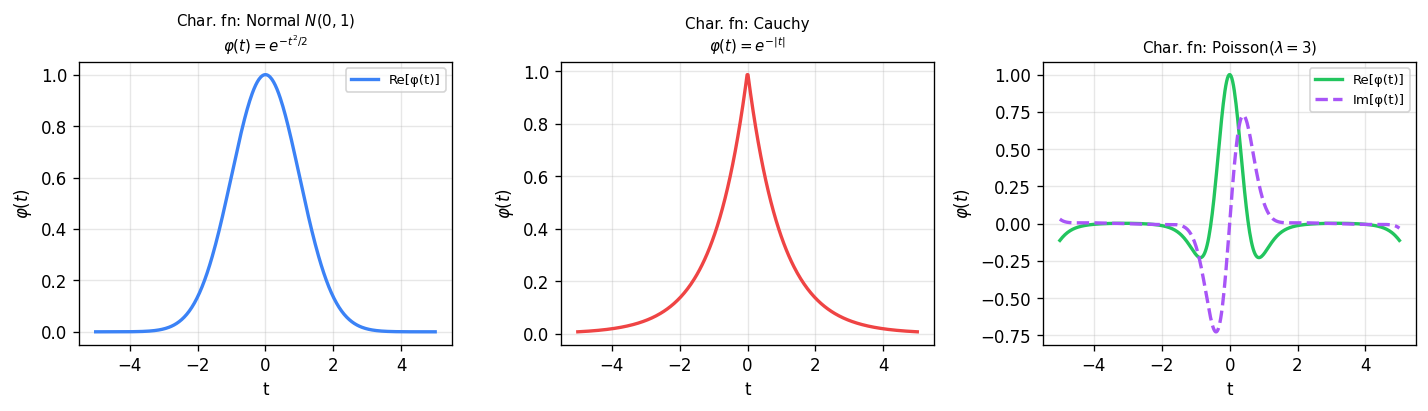
Left: the standard normal characteristic function \(\varphi(t) = e^{-t^2/2}\) — a real-valued Gaussian. Middle: the Cauchy characteristic function \(\varphi(t) = e^{-|t|}\) — a real-valued double-exponential, reflecting the heavy tails of the Cauchy distribution. Right: the Poisson(\(\lambda=3\)) characteristic function — complex-valued with oscillating real and imaginary parts.
- \(\varphi(0) = 1\).
- \(\varphi(-t) = \overline{\varphi(t)}\) (the complex conjugate, where \(\overline{a + bi} = a - bi\)).
- \(|\varphi(t)| = |E[e^{itX}]| \leq E[|e^{itX}|] = 1\).
- \(\varphi_{aX+b}(t) = E[e^{it(aX+b)}] = e^{itb} \varphi_X(at)\).
(2) We have \(\varphi(-t) = E[e^{-itX}] = E[\cos(-tX)] + iE[\sin(-tX)] = E[\cos(tX)] - iE[\sin(tX)]\) since cosine is even and sine is odd.
(3) Note that \(f(x, y) = (x^2 + y^2)^{1/2}\) is a convex function. By Jensen’s inequality, \(f(E[X'], E[Y']) \leq E[f(X', Y')]\). Taking \(X' = \cos(tX)\) and \(Y' = \sin(tX)\), we get \(|\varphi(t)| = f(E[X'], E[Y']) \leq E[f(X', Y')] = E[1] = 1\).
(4) Follows by direct computation. \(\blacksquare\)
The characteristic function behaves multiplicatively for sums of independent random variables, which is its most powerful algebraic property.
Let us illustrate the power of characteristic functions with several important distributions.
If \(Y \sim \operatorname{Poi}(\eta)\) is independent of \(X\), then \(\varphi_{X+Y}(t) = e^{\lambda(e^{it}-1)} e^{\eta(e^{it}-1)} = e^{(\lambda+\eta)(e^{it}-1)}\), which is the characteristic function of a \(\operatorname{Poi}(\lambda + \eta)\) distribution. Thus the sum of independent Poisson random variables is again Poisson.
But does the characteristic function uniquely determine the distribution? The following inversion formula shows that it does.
The cosine terms vanish by symmetry of the integration interval. Using the classical result that for \(\theta > 0\),
\[ \lim_{T \to \infty} \int_{-T}^{T} \frac{\sin(\theta t)}{t} \, dt = \pi, \qquad \lim_{T \to \infty} \int_{-T}^{T} \frac{\sin(\theta t)}{t} \, dt = -\pi \text{ for } \theta < 0, \]we obtain
\[ g(x) := \lim_{T \to \infty} \left[\int_{-T}^{T} \frac{\sin(t(x-a))}{t} \, dt - \int_{-T}^{T} \frac{\sin(t(x-b))}{t} \, dt\right] = \begin{cases} 2\pi & \text{if } a < x < b, \\ \pi & \text{if } x = a \text{ or } x = b, \\ 0 & \text{if } x < a \text{ or } x > b. \end{cases} \]Since \(\left|\int_{-T}^{T} \frac{\sin(t(x-a))}{t} \, dt\right| \leq \sup_c \int_{-c}^{c} \frac{|\sin(y)|}{|y|} \, dy =: M < \infty\), the integrand is bounded by \(2M\). By the Dominated Convergence Theorem, \(\lim_{T \to \infty} I_T = \int g(x) \, \mu(dx) = 2\pi \mu((a,b)) + \pi \mu(\{a,b\})\), and hence \(\frac{1}{2\pi} I_T \to \mu((a,b)) + \frac{1}{2}\mu(\{a,b\})\). \(\blacksquare\)
Here we completed the square and used the fact that the integral of the standard normal density is 1 (by analytic continuation to the complex plane).
If \(X_1 \sim N(\mu_1, \sigma_1^2)\) and \(X_2 \sim N(\mu_2, \sigma_2^2)\) are independent, then
\[ \varphi_{X_1 + X_2}(t) = \exp\left(i(\mu_1 + \mu_2)t - \tfrac{1}{2}(\sigma_1^2 + \sigma_2^2)t^2\right), \]which is the characteristic function of \(N(\mu_1 + \mu_2, \sigma_1^2 + \sigma_2^2)\). By the inversion formula, \(X_1 + X_2 \sim N(\mu_1 + \mu_2, \sigma_1^2 + \sigma_2^2)\).
Multivariate Characteristic Functions and the Multivariate Normal
The theory of characteristic functions extends naturally to random vectors. For a random vector \(\vec{X} = (X_1, \ldots, X_n)\) and any \(\vec{t} = (t_1, \ldots, t_n) \in \mathbb{R}^n\), the multivariate characteristic function is
\[ \varphi_{\vec{X}}(\vec{t}) = E\left[e^{i\langle \vec{t}, \vec{X}\rangle}\right] = E\left[\exp\left(i \sum_{j=1}^n t_j X_j\right)\right] \]where \(\langle \vec{a}, \vec{b}\rangle = \sum_{i=1}^n a_i b_i\) is the standard inner product on \(\mathbb{R}^n\).
The multivariate normal distribution is completely characterized by its mean vector and covariance matrix: \(\vec{X}\) is multivariate normal if and only if its characteristic function has the form
\[ \varphi_{\vec{X}}(\vec{t}) = \exp\left(i\langle \vec{t}, \vec{\mu}\rangle - \tfrac{1}{2} \langle \vec{t}, \Sigma \vec{t}\rangle\right) \]where \(\vec{\mu} = E[\vec{X}] \in \mathbb{R}^n\) and \(\Sigma = (\operatorname{Cov}(X_i, X_j))_{i,j}\) is a symmetric positive semi-definite matrix.
which is the characteristic function of \(N(\langle \vec{a}, \vec{\mu}\rangle, \vec{a}^T \Sigma \vec{a})\). So every linear combination is normal.
(\(\Rightarrow\)) Suppose \(\vec{X}\) is multivariate normal. For any \(\vec{a} \in \mathbb{R}^n\), the variable \(Y = \langle \vec{a}, \vec{X}\rangle\) is normal with mean \(\langle \vec{a}, \vec{\mu}\rangle\) and variance \(\vec{a}^T \Sigma \vec{a}\). Then \(\varphi_{\vec{X}}(\vec{a}) = E[e^{i\langle \vec{a}, \vec{X}\rangle}] = E[e^{i \cdot 1 \cdot Y}] = \varphi_Y(1) = \exp\left(i\langle \vec{a}, \vec{\mu}\rangle - \tfrac{1}{2}\vec{a}^T \Sigma \vec{a}\right)\). \(\blacksquare\)
\(L^p\) Spaces and Further Inequalities
We have already encountered \(L^p\) spaces implicitly through the various notions of integrability. Let us now formalize this concept, as it will be essential for the convergence theory developed in the next chapter.
For a probability space \((\Omega, \mathcal{F}, P)\) and \(1 \leq p < \infty\), the space \(L^p\) consists of all random variables \(X\) such that \(E[|X|^p] < \infty\). This space is equipped with the norm
\[ \|X\|_p = \left(E[|X|^p]\right)^{1/p}. \]The space \(L^2\) is especially important because it is a Hilbert space with inner product \(\langle X, Y \rangle = E[XY]\), which provides the geometric framework for least-squares estimation and projection. Other \(L^p\) spaces for \(p \neq 2\) are Banach spaces (complete normed vector spaces) but do not generally have inner products.
The Markov and Chebyshev inequalities developed earlier are special cases of a more general family of inequalities. Two further inequalities of great importance in the \(L^p\) theory are Holder’s inequality and Minkowski’s inequality.
Holder’s inequality states that if \(p, q > 1\) satisfy \(1/p + 1/q = 1\), and if \(X \in L^p\) and \(Y \in L^q\), then \(XY \in L^1\) and
\[ E[|XY|] \leq \|X\|_p \|Y\|_q. \]The special case \(p = q = 2\) is the Cauchy–Schwarz inequality \(E[|XY|] \leq \sqrt{E[X^2] E[Y^2]}\).
Minkowski’s inequality states that for \(p \geq 1\) and \(X, Y \in L^p\),
\[ \|X + Y\|_p \leq \|X\|_p + \|Y\|_p. \]This is precisely the triangle inequality for the \(L^p\) norm, confirming that \(\|\cdot\|_p\) is indeed a norm on \(L^p\).
Chapter 4: Convergence of Random Variables
In probability theory, we are frequently concerned with the behavior of sequences of random variables. The law of large numbers, the central limit theorem, and the theory of statistical estimation all involve taking limits of random quantities. But what does it mean for a sequence of random variables to “converge”? Unlike sequences of real numbers, where there is only one notion of convergence, sequences of random variables admit several distinct notions of convergence, each capturing a different aspect of probabilistic behavior. In this chapter, we introduce four principal modes of convergence — almost sure, in \(L^p\), in probability, and in distribution — and systematically explore the relationships among them.
Almost Sure Convergence
The strongest and most intuitive notion of convergence requires that, for almost every outcome \(\omega\), the numerical sequence \(X_n(\omega)\) converges to \(X(\omega)\) in the ordinary sense.
Recall that for a sequence of real numbers \(x_1, x_2, \ldots\), the limit exists if and only if \(\limsup_{n \to \infty} x_n = \liminf_{n \to \infty} x_n\). For random variables, the set
\[ \Omega_0 := \{\omega : \lim_{n \to \infty} X_n(\omega) \text{ exists}\} = \{\limsup_{n \to \infty} X_n - \liminf_{n \to \infty} X_n = 0\} \]is measurable (since \(\limsup X_n\) and \(\liminf X_n\) are measurable). If \(P(\Omega_0) = 1\), we say the sequence converges almost surely.
Almost sure convergence means that the set of outcomes where convergence fails has probability zero. For any particular outcome \(\omega\) in the probability-one set, the sequence of real numbers \(X_1(\omega), X_2(\omega), \ldots\) converges to \(X(\omega)\) in the usual sense.
Convergence everywhere is strictly stronger than almost sure convergence, since it requires convergence at every single point, not just on a set of full measure. In practice, almost sure convergence is the more natural and useful concept.
Convergence in \(L^p\)
While almost sure convergence is about the pointwise behavior of sample paths, convergence in \(L^p\) is about the behavior of integral (expectation) quantities.
Two important special cases deserve emphasis. If \(X_n \xrightarrow{L^1} X\), then \(E[|X_n - X|] \to 0\), which implies \(E[X_n] \to E[X]\); this is necessary but not sufficient for \(L^1\) convergence. If \(X_n \xrightarrow{L^2} X\), then \(E[(X_n - X)^2] \to 0\), which implies \(E[X_n^2] \to E[X^2]\); again necessary but not sufficient. The space \(L^2\) is especially tractable because it is a Hilbert space with inner product structure, while other \(L^p\) spaces are Banach spaces without inner products.
Convergence in Probability
Convergence in probability is a weaker notion that asks only that the probability of a large deviation tends to zero, without requiring that deviations vanish along individual sample paths.
Relationships Among the Modes of Convergence
The following theorem establishes the two most basic implications among our modes of convergence.
- If \(X_n \xrightarrow{a.s.} X\), then \(X_n \xrightarrow{P} X\).
- If \(X_n \xrightarrow{L^p} X\), then \(X_n \xrightarrow{P} X\).
Since \(P(\{X_n \to X\}) = 1\), by continuity of probability, \(\lim_{n \to \infty} P(A_n) = 1\). Since \(A_n \subseteq \{|X_n - X| \leq \varepsilon\}\), we get \(\lim_{n \to \infty} P(|X_n - X| \leq \varepsilon) = 1\).
(2) Fix \(\varepsilon > 0\). By the Markov inequality,
\[ P(|X_n - X| > \varepsilon) = P(|X_n - X|^p > \varepsilon^p) \leq \frac{E[|X_n - X|^p]}{\varepsilon^p} \to 0 \]since \(X_n \xrightarrow{L^p} X\). \(\blacksquare\)
Higher \(L^p\) convergence implies lower \(L^p\) convergence:
When \(|X_n - X| \geq \varepsilon\), we have \(|X_n - X|^p \leq \varepsilon^{p-q} |X_n - X|^q\) since \(p - q < 0\). When \(|X_n - X| < \varepsilon\), we have \(|X_n - X|^p < \varepsilon^p\). Therefore
\[ E[|X_n - X|^p] \leq \varepsilon^{p-q} E[|X_n - X|^q] + \varepsilon^p. \]Taking \(n \to \infty\), \(\limsup_{n \to \infty} E[|X_n - X|^p] \leq \varepsilon^p\). Since \(\varepsilon > 0\) is arbitrary, the result follows. \(\blacksquare\)
The converses of the implications in Theorem 42 are false in general, as the following examples demonstrate.
Although convergence in probability does not imply almost sure convergence, it does imply the existence of an almost surely convergent subsequence.
By the first Borel–Cantelli lemma, \(P(|X_{i_m} - X| > 1/m \text{ i.o.}) = 0\). This means that \(|X_{i_m} - X| > 1/m\) for only finitely many \(m\) almost surely, which in turn means \(|X_{i_m} - X| \leq 1/m\) from some \(m\) onward almost surely. Therefore \(X_{i_m} \xrightarrow{a.s.} X\). \(\blacksquare\)
Uniform Integrability
We have seen that convergence in probability does not in general imply \(L^p\) convergence. The missing condition is uniform integrability, which controls the tails of the distributions uniformly over the sequence.
Intuitively, uniform integrability means that the “tail mass” of the integrals is uniformly small: as the truncation threshold \(k\) grows, the contribution of \(|X_n|\) beyond \(k\) vanishes, uniformly over all \(n\). For a single integrable random variable, the tail contribution always vanishes; uniform integrability requires this to happen at the same rate for the entire sequence. The counterexample \(X_n = n \mathbf{1}_{(0,1/n)}\) fails uniform integrability because the integrals do not grow “nicely” — the mass concentrates on a shrinking set but grows proportionally taller.
Since this holds for all \(\varepsilon > 0\), \(E[|X_n|] \to 0\), so \(X_n \xrightarrow{L^1} 0\). \(\blacksquare\)
Convergence in Distribution
The weakest mode of convergence does not involve the random variables themselves, only their distribution functions. It is also the most widely applicable, forming the basis for the central limit theorem and asymptotic statistics.
for \(x \geq 0\). Thus \(P(pX_p \leq x) \to 1 - e^{-x}\), the c.d.f. of an \(\operatorname{Exp}(1)\) distribution. So \(pX_p \xrightarrow{d} W\) where \(W \sim \operatorname{Exp}(1)\).
Convergence in probability implies convergence in distribution, as the following result shows.
For such \(n\), \(F_n(a) = P(X_n \leq a) = P(X_n \leq a, |X_n - X| \leq \delta) + P(X_n \leq a, |X_n - X| > \delta)\). The second term is at most \(\varepsilon\). The first term satisfies
\[ P(X_n \leq a, |X_n - X| \leq \delta) \in \left[F(a - \delta) - \varepsilon,\; F(a + \delta)\right]. \]Thus \(F_n(a) \in (F(a) - 2\varepsilon, F(a) + 2\varepsilon)\). Since \(\varepsilon\) is arbitrary, \(F_n(a) \to F(a)\). \(\blacksquare\)
The converse is false in general: convergence in distribution does not imply convergence in probability. However, there is one important exception.
Skorokhod’s Theorem
A remarkable result due to Skorokhod shows that convergence in distribution can always be “upgraded” to almost sure convergence on a suitable probability space. This theorem is a powerful technical tool for transferring results from almost sure convergence to the distributional setting.
For any \(x \in (0,1)\), define \(a_x = \sup\{y : F(y) < x\}\) and \(b_x = \inf\{y : F(y) > x\}\). Let \(\Omega_0 = \{x : a_x = b_x\}\). For \(x \in \Omega_0\), if \(y < F^{-1}(x)\) then \(F(y) < x\), and if \(y > F^{-1}(x)\) then \(F(y) > x\).
We claim that for any \(x \in \Omega_0\): (1) \(\liminf_{n \to \infty} F_n^{-1}(x) \geq F^{-1}(x)\), and (2) \(\limsup_{n \to \infty} F_n^{-1}(x) \leq F^{-1}(x)\).
For (1), let \(y < F^{-1}(x)\) be a continuity point of \(F\). Then \(F(y) < x\). By weak convergence, \(F_n(y) \to F(y) < x\), so \(F_n(y) < x\) for large \(n\), hence \(y \leq F_n^{-1}(x)\). Taking \(y \to F^{-1}(x)\) from below gives (1). Claim (2) follows by a similar argument.
Since \(\Omega \setminus \Omega_0\) is at most countable (each element corresponds to a distinct non-degenerate interval, and each such interval contains a rational number), \(P(\Omega \setminus \Omega_0) = 0\). Thus \(Y_n \xrightarrow{a.s.} Y\). \(\blacksquare\)
Skorokhod’s theorem is enormously useful because it allows us to use pointwise convergence arguments (and thus the Dominated Convergence Theorem) in situations where we only have convergence in distribution. We will see it applied immediately in the proof of the Portmanteau theorem.
The Portmanteau Theorem
The Portmanteau theorem provides several equivalent characterizations of weak convergence. It is one of the central results in the theory and is used constantly in asymptotic statistics.
- \(X_n \xrightarrow{d} X\).
- \(E[f(X_n)] \to E[f(X)]\) for all bounded continuous functions \(f\).
- \(\mu_n(A) \to \mu(A)\) for every \(\mu\)-continuity set \(A\), where \(\mu_n\) and \(\mu\) are the probability measures induced by \(X_n\) and \(X\). Equivalently, \(P(X_n \in A) \to P(X \in A)\) for all sets \(A\) with \(P(X \in \partial A) = 0\).
(1) \(\Rightarrow\) (2): Let \(f\) be bounded and continuous. By Skorokhod’s theorem, there exist \(Y_1, Y_2, \ldots\) and \(Y\) with \(Y_n \overset{D}{=} X_n\), \(Y \overset{D}{=} X\), and \(Y_n \xrightarrow{a.s.} Y\). Then \(E[f(Y_n)] = E[f(X_n)]\) and \(E[f(Y)] = E[f(X)]\). Since \(f\) is continuous and \(Y_n \xrightarrow{a.s.} Y\), we have \(f(Y_n) \xrightarrow{a.s.} f(Y)\). Since \(f\) is bounded, the Dominated Convergence Theorem gives \(E[f(Y_n)] \to E[f(Y)]\).
(1) \(\Rightarrow\) (3): A similar argument applies using \(f = \mathbf{1}_A\). Since \(A\) is a \(\mu\)-continuity set, \(P(Y \in \partial A) = P(X \in \partial A) = 0\), so \(f\) is almost surely continuous for \(Y\). Since \(Y_n \xrightarrow{a.s.} Y\), we still get \(f(Y_n) \xrightarrow{a.s.} f(Y)\), and since \(f\) is bounded, DCT applies.
(3) \(\Rightarrow\) (1): Take \(A = (-\infty, x]\), so \(\partial A = \{x\}\). Then \(A\) is a \(\mu\)-continuity set if and only if \(P(X = x) = 0\), which holds if and only if \(F\) is continuous at \(x\). So \(F_n(x) \to F(x)\) at all continuity points of \(F\).
(2) \(\Rightarrow\) (1): For any \(x\) at which \(F\) is continuous and any \(y > x\), define the piecewise linear function
\[ f(t) = \begin{cases} 1 & \text{if } t \leq x, \\ \frac{y - t}{y - x} & \text{if } x < t < y, \\ 0 & \text{if } t \geq y, \end{cases} \]which is bounded and continuous. Note \(F_n(x) = E[\mathbf{1}_{(-\infty, x]}(X_n)] \leq E[f(X_n)]\) and \(E[f(X)] \leq F(y)\). By (2), taking \(n \to \infty\) gives \(\limsup F_n(x) \leq F(y)\). Since \(F\) is continuous at \(x\), taking \(y \to x^+\) gives \(\limsup F_n(x) \leq F(x)\). A similar argument with \(y < x\) gives \(F(x) \leq \liminf F_n(x)\). Hence \(F_n(x) \to F(x)\). \(\blacksquare\)
Characterization (2) is often taken as the definition of weak convergence in more general settings (e.g., for random elements of metric spaces), where distribution functions may not be available.
The Continuous Mapping Theorem
A direct consequence of Skorokhod’s theorem is the continuous mapping theorem, which states that continuous functions preserve convergence in distribution.
Slutsky’s Theorem
An important companion to the continuous mapping theorem is Slutsky’s theorem, which describes how convergence in distribution interacts with convergence in probability. It is used constantly in asymptotic statistics.
This follows because convergence in probability to zero can be combined with convergence in distribution to yield convergence in distribution of the perturbed sequence. More generally, if \(X_n \xrightarrow{d} X\) and \(Y_n \xrightarrow{P} c\) for a constant \(c\), then \(X_n + Y_n \xrightarrow{d} X + c\) and \(X_n Y_n \xrightarrow{d} cX\). The key requirement is that the sequence converging in probability must converge to a constant, not to a random variable.
Helly’s Selection Theorem
We now turn to the question of compactness for sequences of distribution functions. Helly’s selection theorem is the analogue of the Bolzano–Weierstrass theorem for distribution functions: it guarantees that every sequence of distribution functions has a subsequence that converges, at least in a weak sense.
Since each \(F_n\) is non-decreasing, \(G\) is also non-decreasing. To make \(G\) right-continuous, define \(F(x) := \inf\{G(q) : q \in \mathbb{Q}, q > x\}\). Then \(F\) is right-continuous and non-decreasing.
It remains to show \(F_{n_k(k)}(x) \to F(x)\) at all continuity points of \(F\). Let \(\varepsilon > 0\). Choose rational \(r_1 < r_2 < x < s\) with \(F(x) - \varepsilon < F(r_1) \leq F(r_2) \leq F(x) \leq F(s) < F(x) + \varepsilon\). Since \(F_{n_k(k)}(s) \to G(s) \leq F(s) < F(x) + \varepsilon\), for large \(k\), \(F_{n_k(k)}(x) \leq F_{n_k(k)}(s) < F(x) + \varepsilon\). Since \(F_{n_k(k)}(r_2) \to G(r_2) \geq F(r_1) > F(x) - \varepsilon\), for large \(k\), \(F_{n_k(k)}(x) \geq F_{n_k(k)}(r_2) > F(x) - \varepsilon\). Thus \(|F_{n_k(k)}(x) - F(x)| < \varepsilon\) for large \(k\). \(\blacksquare\)
Tightness
Tightness is the condition that prevents mass from escaping to infinity along subsequences. It is the key ingredient that upgrades Helly’s selection theorem from a statement about non-decreasing functions to a statement about distribution functions.
The fundamental theorem connecting tightness and weak convergence is Prokhorov’s theorem, one direction of which is established here.
(\(\Leftarrow\)) By contrapositive, if the sequence is not tight, there exist \(\varepsilon > 0\) and indices \(n(k) \to \infty\) with \(1 - F_{n(k)}(k) + F_{n(k)}(-k) \geq \varepsilon\). By Helly, any further subsequence converges to some \(F\), but the tightness failure forces \(\lim_{y \to \infty}(F(y) - F(-y)) \leq 1 - \varepsilon\), so \(F\) cannot be a distribution function. \(\blacksquare\)
The Continuity Theorem
The continuity theorem is the cornerstone of the characteristic function approach to convergence in distribution. It states that weak convergence of probability measures is equivalent to pointwise convergence of characteristic functions, providing a powerful analytic tool for proving distributional limit theorems.
(\(\Leftarrow\)) We first show tightness. Using the identity
\[ \frac{1}{u} \int_{-u}^{u} (1 - \varphi_n(t)) \, dt = 2E\left[1 - \frac{\sin(uX_n)}{uX_n}\right] \geq P\left(|X_n| \geq \frac{2}{u}\right), \]which holds because \(|\sin(x)/x| \leq 1\) and \(1 - \sin(x)/x \geq 1/2\) when \(|x| \geq 2\). Since \(\varphi\) is continuous with \(\varphi(0) = 1\), for any \(\varepsilon > 0\) there exists \(u > 0\) with \(u^{-1} \int_{-u}^{u} (1 - \varphi(t)) \, dt < \varepsilon\). Since \(\varphi_n \to \varphi\) pointwise and \(|1 - \varphi_n(t)| \leq 2\), by DCT, \(u^{-1}\int_{-u}^{u}(1 - \varphi_n(t)) \, dt \to u^{-1}\int_{-u}^{u}(1 - \varphi(t)) \, dt\). So for large \(n\), \(u^{-1}\int_{-u}^{u}(1 - \varphi_n(t)) \, dt < \varepsilon\), giving \(P(|X_n| \geq 2/u) < \varepsilon\). This establishes tightness.
Now suppose a subsequence \(\mu_{n_k}\) converges weakly to some \(\mu'\). By the forward direction, \(\varphi_{n_k}(t) \to \varphi'(t)\). But \(\varphi_{n_k}(t) \to \varphi(t)\), so \(\varphi' = \varphi\). Since the characteristic function determines the distribution, \(\mu' = \mu\). All weakly convergent subsequences have the same limit, so by Corollary 52, \(\mu_n \xrightarrow{d} \mu\). \(\blacksquare\)
The continuity theorem is the engine behind most proofs of the central limit theorem: one shows that the characteristic functions of the standardized sample means converge pointwise to \(e^{-t^2/2}\), the characteristic function of the standard normal, and then invokes the continuity theorem to conclude convergence in distribution.
Summary of Relationships
We conclude this chapter with a summary of the relationships among the four modes of convergence for a sequence of random variables \(X_n\) and a limit \(X\):
- \(X_n \xrightarrow{a.s.} X \implies X_n \xrightarrow{P} X \implies X_n \xrightarrow{d} X\).
- \(X_n \xrightarrow{L^p} X \implies X_n \xrightarrow{P} X \implies X_n \xrightarrow{d} X\).
- For \(1 \leq p < q < \infty\): \(X_n \xrightarrow{L^q} X \implies X_n \xrightarrow{L^p} X\).
- \(X_n \xrightarrow{P} X\) implies there exists a subsequence \(X_{n_k} \xrightarrow{a.s.} X\).
- \(X_n \xrightarrow{P} X\) with \(\{X_n\}\) uniformly integrable implies \(X_n \xrightarrow{L^1} X\).
- \(X_n \xrightarrow{d} c\) (constant) implies \(X_n \xrightarrow{P} c\).
- There is no general implication between almost sure convergence and \(L^p\) convergence in either direction.
These relationships form a web of connections that pervades all of probability theory and mathematical statistics. Understanding which mode of convergence is appropriate in a given context — and what additional conditions are needed to strengthen one mode to another — is a central skill in modern probability.
Chapter 5: Characteristic Functions and Limit Theorems
The deepest results in probability theory concern the large-scale behaviour of sums of random variables. The law of large numbers asserts that averages converge to their expected values; the central limit theorem explains that the fluctuations around those averages are approximately Gaussian. To prove these results in full generality we need a tool that converts the multiplicative structure of independence into something analytically tractable. That tool is the characteristic function, which exists for every distribution and uniquely determines it.
This chapter begins with the definition and fundamental properties of characteristic functions, including the inversion formula and the continuity theorem that links pointwise convergence of characteristic functions to weak convergence of distributions. Armed with these tools we then prove the weak and strong laws of large numbers and the central limit theorem, culminating in the Lindeberg–Feller extension and the delta method.
Characteristic Functions
Definition and Basic Properties
Recall that the moment generating function \( M_X(t) = E[e^{tX}] \) does not always exist: the integral may diverge when the tails of the distribution are heavy. The key advantage of the characteristic function is that it replaces the real exponential with the complex exponential \( e^{itX} \), which always has modulus one.
The characteristic function is sometimes called the Fourier–Stieltjes transform of the distribution. Unlike the moment generating function or the probability generating function, the characteristic function always exists on all of \( \mathbb{R} \) because \( |e^{itx}| = 1 \) for every real \( t \) and \( x \), so the integral is dominated by the constant function 1, which is integrable with respect to any probability measure. This universality is the reason we prefer characteristic functions when proving general distributional results.
- \( \varphi(0) = 1 \).
- \( \varphi(-t) = \overline{\varphi(t)} \) (the complex conjugate).
- \( |\varphi(t)| \leq 1 \) for all \( t \in \mathbb{R} \).
- If \( Y = aX + b \) for constants \( a, b \in \mathbb{R} \), then \( \varphi_Y(t) = e^{ibt}\,\varphi_X(at) \).
- \( \varphi \) is uniformly continuous on \( \mathbb{R} \).
- The characteristic function of \( -X \) is \( \overline{\varphi(t)} \).
- \( \varphi \) is real-valued if and only if the distribution of \( X \) is symmetric about zero.
- If \( X \) and \( Y \) are independent, then \( \varphi_{X+Y}(t) = \varphi_X(t)\,\varphi_Y(t) \).
Property (4) is a direct calculation: \( E[e^{it(aX+b)}] = e^{ibt}\,E[e^{i(at)X}] = e^{ibt}\,\varphi_X(at) \).
For (5), let \( h = s - t \). Then
\[ |\varphi(t) - \varphi(s)| = |E[e^{itX}(e^{ihX} - 1)]| \leq E[|e^{ihX} - 1|]. \]As \( h \to 0 \), the function \( e^{ihX} - 1 \to 0 \) pointwise, and it is bounded by 2. By the dominated convergence theorem, \( E[|e^{ihX} - 1|] \to 0 \), so \( \varphi \) is uniformly continuous.
Property (6) is the same as (2). For (7), the distribution is symmetric about zero precisely when \( X \) and \( -X \) have the same distribution, hence the same characteristic function. By (6), this means \( \varphi(t) = \overline{\varphi(t)} \), which holds if and only if \( \varphi \) is real-valued.
For (8), independence gives
\[ \varphi_{X+Y}(t) = E[e^{it(X+Y)}] = E[e^{itX}\,e^{itY}] = E[e^{itX}]\,E[e^{itY}] = \varphi_X(t)\,\varphi_Y(t). \qquad \blacksquare \]Property (8) is especially powerful: it converts the convolution of distributions (which is analytically cumbersome) into a simple product. This is the fundamental reason characteristic functions are useful for studying sums of independent random variables.
Examples
The Poisson and normal characteristic functions illustrate the technique and will be used repeatedly in the sequel.
If \( Y \sim \mathrm{Poi}(\eta) \) is independent of \( X \), then \( \varphi_{X+Y}(t) = e^{(\lambda+\eta)(e^{it}-1)} \), which is the characteristic function of a \( \mathrm{Poi}(\lambda + \eta) \). Does this guarantee \( X + Y \sim \mathrm{Poi}(\lambda+\eta) \)? It does, provided the characteristic function uniquely determines the distribution – a fact we establish next.
More generally, if \( X \sim N(\mu, \sigma^2) \), then \( X = \mu + \sigma Z \) and property (4) gives
\[ \varphi_X(t) = e^{i\mu t - \sigma^2 t^2/2}. \]Since characteristic functions multiply under convolution of independent summands, the sum of independent normals \( X_1 \sim N(\mu_1, \sigma_1^2) \) and \( X_2 \sim N(\mu_2, \sigma_2^2) \) has characteristic function \( \exp(i(\mu_1+\mu_2)t - \tfrac{1}{2}(\sigma_1^2+\sigma_2^2)t^2) \), which is that of \( N(\mu_1+\mu_2, \sigma_1^2+\sigma_2^2) \).
The Inversion Formula
The inversion formula shows how to recover probabilities from the characteristic function, thereby establishing that the characteristic function uniquely determines the distribution.
The proof proceeds by interchanging the order of integration (justified by Fubini’s theorem), reducing the problem to the evaluation of the sine integral.
By Fubini’s theorem (noting that the integrand is bounded), we may interchange the order of integration to obtain
\[ I_T = \int_{\mathbb{R}}\int_{-T}^{T}\frac{e^{it(x-a)} - e^{it(x-b)}}{it}\,dt\,\mu(dx). \]The inner integral separates into sine integrals. Since \( \frac{e^{itc}}{i} \) has real part \( \frac{\sin(tc)}{t} \) (the cosine terms cancel by symmetry of the interval \( [-T,T] \)), we get
\[ I_T = \int_{\mathbb{R}}\left[\int_{-T}^{T}\frac{\sin(t(x-a))}{t}\,dt - \int_{-T}^{T}\frac{\sin(t(x-b))}{t}\,dt\right]\mu(dx). \]The classical result \( \int_{-\infty}^{\infty}\frac{\sin(y)}{y}\,dy = \pi \) (and the substitution \( y = \theta t \)) gives, for \( \theta > 0 \),
\[ \lim_{T\to\infty}\int_{-T}^{T}\frac{\sin(\theta t)}{t}\,dt = \pi, \qquad \lim_{T\to\infty}\int_{-T}^{T}\frac{\sin(\theta t)}{t}\,dt = -\pi \text{ for } \theta < 0. \]Therefore, define
\[ g(x) = \lim_{T\to\infty}\left[\int_{-T}^{T}\frac{\sin(t(x-a))}{t}\,dt - \int_{-T}^{T}\frac{\sin(t(x-b))}{t}\,dt\right] = \begin{cases} 2\pi & \text{if } a < x < b, \\ \pi & \text{if } x = a \text{ or } x = b, \\ 0 & \text{if } x < a \text{ or } x > b. \end{cases} \]Since the integrand is bounded by a universal constant \( 2M \) (where \( M = \sup_{c}\int_{-c}^{c}\frac{|\sin y|}{|y|}\,dy < \infty \)), the dominated convergence theorem justifies passing the limit inside the outer integral:
\[ \lim_{T\to\infty} I_T = \int_{\mathbb{R}} g(x)\,\mu(dx) = 2\pi\,\mu((a,b)) + \pi\,\mu(\{a,b\}). \]Dividing by \( 2\pi \) yields the result. \( \blacksquare \)
The most important consequence of the inversion formula is that the characteristic function completely determines the distribution.
This follows immediately from the inversion formula, since the probabilities of all intervals \( (a,b) \) are determined by \( \varphi \), and these generate the Borel \( \sigma \)-algebra.
We also record the multivariate extension.
for \( \mathbf{t} = (t_1, \ldots, t_n) \in \mathbb{R}^n \). The multivariate inversion and uniqueness theorems hold by the same arguments applied coordinate-wise.
The Lévy Continuity Theorem
The continuity theorem is the bridge between characteristic functions and weak convergence. It asserts that pointwise convergence of characteristic functions to a limit that is continuous at the origin is equivalent to weak convergence of the corresponding distributions.
The forward direction is a straightforward application of the portmanteau theorem; the converse requires establishing tightness of the sequence from the assumed pointwise convergence.
Converse. Assume \( \varphi_n(t) \to \varphi(t) \) for all \( t \) and that \( \varphi \) is continuous at 0 (which it is, being the characteristic function of a probability measure). We first show the sequence \( \{\mu_n\} \) is tight. Observe that
\[ \frac{1}{u}\int_{-u}^{u}(1 - \varphi_n(t))\,dt = 2\,E\!\left[1 - \frac{\sin(uX_n)}{uX_n}\right]. \]Since \( 1 - \frac{\sin(y)}{y} \geq 0 \) and \( 1 - \frac{\sin(y)}{y} \geq \frac{1}{2} \) whenever \( |y| \geq 2 \), we obtain
\[ \frac{1}{u}\int_{-u}^{u}(1 - \varphi_n(t))\,dt \geq P\!\left(|X_n| \geq \frac{2}{u}\right). \]Because \( \varphi \) is continuous and \( \varphi(0) = 1 \), we have \( u^{-1}\int_{-u}^{u}(1-\varphi(t))\,dt \to 0 \) as \( u \to 0 \). Since \( \varphi_n \to \varphi \) pointwise and \( |1-\varphi_n(t)| \leq 2 \), the dominated convergence theorem gives
\[ \frac{1}{u}\int_{-u}^{u}(1-\varphi_n(t))\,dt \to \frac{1}{u}\int_{-u}^{u}(1-\varphi(t))\,dt. \]Hence, for any \( \varepsilon > 0 \), choose \( u \) small enough that the right side is less than \( \varepsilon \), then choose \( N \) large enough so that the left side is also less than \( \varepsilon \) for all \( n \geq N \). Setting \( M = 2/u \), we get \( P(|X_n| \geq M) < \varepsilon \) for all large \( n \). This establishes tightness.
By Helly’s selection theorem, every subsequence of \( \{\mu_n\} \) has a further subsequence that converges weakly to some probability measure \( \mu' \). By the forward direction, the characteristic function of \( \mu' \) must equal \( \varphi \). Since characteristic functions uniquely determine distributions, \( \mu' = \mu \). Thus every weakly convergent subsequence has the same limit \( \mu \), which implies \( \mu_n \xrightarrow{d} \mu \). \( \blacksquare \)
Taylor Expansion of Characteristic Functions
Before proving the central limit theorem, we need a precise expansion of the characteristic function in terms of moments.
Applying this lemma with \( n = 2 \) and taking expectations yields the following.
as \( t \to 0 \).
The quantity inside the expectation converges to 0 as \( t \to 0 \) and is bounded by \( |X|^2 \), which is integrable. By the dominated convergence theorem, the expectation is \( o(1) \), and multiplying by \( t^2 \) gives \( o(t^2) \). \( \blacksquare \)
Laws of Large Numbers
The laws of large numbers assert that the sample mean converges to the population mean. We present a hierarchy of results, starting with the simplest \( L^2 \) version and progressing to the general strong law.
Weak Law of Large Numbers: \( L^2 \) Version
The simplest convergence result requires only uncorrelated random variables with uniformly bounded variances.
Thus \( \frac{S_n}{n} \to \mu \) in \( L^2 \), which implies convergence in probability. \( \blacksquare \)
Triangular Array Version
Many applications involve arrays of random variables rather than a single sequence. The following extension handles this setting.
Truncation Method
The following result uses truncation to weaken the moment assumptions. The idea is to replace the original random variables by truncated versions, verify convergence of the truncated sums, and then show that the truncation error is negligible.
- \( \sum_{k=1}^{n}P(|X_{n,k}| > b_n) \to 0 \), and
- \( b_n^{-2}\sum_{k=1}^{n}E[\tilde{X}_{n,k}^2] \to 0 \).
For the first term, \( P(S_n \neq \tilde{S}_n) \leq \sum_{k=1}^{n}P(X_{n,k} \neq \tilde{X}_{n,k}) = \sum_{k=1}^{n}P(|X_{n,k}| > b_n) \to 0 \) by condition (1). Since \( a_n = E[\tilde{S}_n] \), the second term satisfies
\[ E\!\left[\left(\frac{\tilde{S}_n - a_n}{b_n}\right)^2\right] = \frac{\operatorname{Var}(\tilde{S}_n)}{b_n^2} = \frac{1}{b_n^2}\sum_{k=1}^{n}\operatorname{Var}(\tilde{X}_{n,k}) \leq \frac{1}{b_n^2}\sum_{k=1}^{n}E[\tilde{X}_{n,k}^2] \to 0 \]by condition (2). Hence both terms vanish, giving \( \frac{S_n - a_n}{b_n} \xrightarrow{P} 0 \). \( \blacksquare \)
The following auxiliary result is needed for the verification of condition (2) in practice.
where the interchange of integral and expectation is justified by Fubini’s theorem. \( \blacksquare \)
Now we can prove the classical weak law requiring only finite first moments.
Since \( y\,P(|X_1| > y) \to 0 \), the running average \( \frac{1}{n}\int_0^{n}2y\,P(|X_1| > y)\,dy \to 0 \). The result then follows from the truncation theorem. \( \blacksquare \)
by the dominated convergence theorem (since \( |X_1|\,\mathbf{1}_{\{|X_1| > x\}} \leq |X_1| \) and \( |X_1|\,\mathbf{1}_{\{|X_1| > x\}} \to 0 \) a.s.). Moreover, \( \mu_n = E[X_1\,\mathbf{1}_{\{|X_1| \leq n\}}] \to E[X_1] = \mu \) by dominated convergence. Therefore
\[ \frac{S_n}{n} - \mu = \left(\frac{S_n}{n} - \mu_n\right) + (\mu_n - \mu) \xrightarrow{P} 0. \qquad \blacksquare \]Strong Law of Large Numbers
The strong law strengthens convergence in probability to almost sure convergence. The proof is considerably more involved, requiring Borel–Cantelli arguments and careful bounding of variances along subsequences. We need two preparatory lemmas.
by Fubini’s theorem. By the previous lemma, \( 2y\sum_{k>y}k^{-2} \leq 4 \), so
\[ \sum_{k=1}^{\infty}\frac{E[Y_k^2]}{k^2} \leq 4\int_0^{\infty}P(|X_1|>y)\,dy = 4\,E[|X_1|] < \infty. \qquad \blacksquare \]Step 2: Convergence along a subsequence. Fix \( \alpha > 1 \) and let \( k(n) = \lfloor\alpha^n\rfloor \). By Chebyshev’s inequality,
\[ \sum_{n=1}^{\infty}P(|T_{k(n)} - E[T_{k(n)}]| > \varepsilon\,k(n)) \leq \varepsilon^{-2}\sum_{n=1}^{\infty}\frac{\operatorname{Var}(T_{k(n)})}{k(n)^2}. \]Interchanging the order of summation,
\[ \sum_{n=1}^{\infty}\frac{\operatorname{Var}(T_{k(n)})}{k(n)^2} = \sum_{n=1}^{\infty}\frac{1}{k(n)^2}\sum_{m=1}^{k(n)}\operatorname{Var}(Y_m) = \sum_{m=1}^{\infty}\operatorname{Var}(Y_m)\sum_{n:\,k(n)\geq m}\frac{1}{k(n)^2}. \]Since \( k(n) \geq \alpha^n/2 \) for \( n \geq 1 \), the inner sum is bounded by \( 4\alpha^{-2n_0} \cdot \frac{1}{1-\alpha^{-2}} \leq \frac{4}{m^2(1-\alpha^{-2})} \). Therefore,
\[ \sum_{n=1}^{\infty}\frac{\operatorname{Var}(T_{k(n)})}{k(n)^2} \leq \frac{4}{1-\alpha^{-2}}\sum_{m=1}^{\infty}\frac{\operatorname{Var}(Y_m)}{m^2} \leq \frac{16\,E[|X_1|]}{1-\alpha^{-2}} < \infty. \]By the first Borel–Cantelli lemma, \( P(|T_{k(n)} - E[T_{k(n)}]|/k(n) > \varepsilon \ \text{i.o.}) = 0 \), so almost surely \( (T_{k(n)} - E[T_{k(n)}])/k(n) \to 0 \). Since \( E[Y_k] \to E[X_1] = \mu \) by dominated convergence, Cesàro’s theorem gives \( E[T_{k(n)}]/k(n) \to \mu \). Combining: \( T_{k(n)}/k(n) \to \mu \) a.s.
Step 3: Extension to the full sequence. Since \( X \geq 0 \), \( T_n \) is non-decreasing. For any \( m \), choose \( n \) so that \( k(n) \leq m \leq k(n+1) \). Then
\[ \frac{T_{k(n)}}{k(n+1)} \leq \frac{T_m}{m} \leq \frac{T_{k(n+1)}}{k(n)}. \]Since \( k(n+1)/k(n) \to \alpha \), taking limits gives
\[ \frac{\mu}{\alpha} \leq \liminf_{m\to\infty}\frac{T_m}{m} \leq \limsup_{m\to\infty}\frac{T_m}{m} \leq \alpha\mu. \]Letting \( \alpha \to 1 \), we conclude \( T_m/m \to \mu \) a.s. \( \blacksquare \)
Applications of the Strong Law
As \( t \to \infty \), \( N_t \to \infty \), so both sides converge to \( \mu \) a.s. Hence \( t/N_t \to \mu \), i.e., \( N_t/t \to 1/\mu \). \( \blacksquare \)
The Glivenko–Cantelli Theorem
The Glivenko–Cantelli theorem is a beautiful application of the strong law that establishes uniform convergence of the empirical distribution function.
For each \( k \geq 1 \) and \( 1 \leq j \leq k-1 \), define \( x_{j,k} = \inf\{y : F(y) \geq j/k\} \), the \( (j/k) \)th quantile. By construction, \( F(x_{j,k}-) - F(x_{j-1,k}) \leq 1/k \). By almost sure pointwise convergence, almost surely there exists \( N_k(\omega) \) such that for all \( n \geq N_k(\omega) \),
\[ |F_n(x_{j,k}) - F(x_{j,k})| < \frac{1}{k} \quad \text{and} \quad |F_n(x_{j,k}-) - F(x_{j,k}-)| < \frac{1}{k} \]for all \( 1 \leq j \leq k-1 \). For any \( x \in [x_{j-1,k}, x_{j,k}) \), since \( F_n \) and \( F \) are both non-decreasing,
\[ F_n(x) \leq F_n(x_{j,k}-) \leq F(x_{j,k}-) + \frac{1}{k} \leq F(x) + \frac{2}{k}, \]and similarly \( F_n(x) \geq F(x) - \frac{2}{k} \). Thus \( \sup_x|F_n(x) - F(x)| \leq 2/k \) for \( n \geq N_k(\omega) \). Since this holds for all \( k \), taking \( k \to \infty \) gives the result. \( \blacksquare \)
The Central Limit Theorem
Having established that averages converge, we now ask about the rate of convergence. The central limit theorem asserts that the standardized fluctuations are asymptotically Gaussian.
as \( n \to \infty \). Since \( e^{-t^2/2} \) is the characteristic function of the standard normal distribution and is continuous at the origin, the Lévy continuity theorem gives the result. \( \blacksquare \)
For instance, when \( p = 1/2 \) and \( n = 10000 \),
\[ P(4900 \leq S_n \leq 5100) \approx \Phi(2) - \Phi(-2) \approx 0.95. \]This is the basis for the normal approximation to the binomial that is widely used in practice.
The Lindeberg–Feller CLT
The classical CLT requires the summands to be identically distributed. The Lindeberg–Feller theorem relaxes this requirement, allowing the summands to vary across rows of a triangular array.
- \( \sum_{m=1}^{n}E[X_{n,m}^2] \to \sigma^2 > 0 \), and
- for every \( \varepsilon > 0 \), \( \displaystyle\lim_{n\to\infty}\sum_{m=1}^{n}E\!\left[|X_{n,m}|^2\,\mathbf{1}_{\{|X_{n,m}| > \varepsilon\}}\right] = 0 \).
Condition (2) is called the Lindeberg condition: it requires that no single summand contributes a disproportionate share of the total variance, which is the essential requirement for asymptotic normality. Intuitively, the central limit theorem holds whenever the aggregate effect arises from many small, independent contributions.
The Delta Method
The delta method is a useful technique for determining the asymptotic distribution of a smooth function of a sequence of random variables that satisfies a CLT. Although it was not explicitly covered in the STAT 901 lectures, it is a natural and important consequence of the central limit theorem.
Since \( X_n \xrightarrow{P} \theta \) (convergence in distribution to a constant implies convergence in probability), the remainder \( o(|X_n - \theta|) \) is negligible after multiplication by \( \sqrt{n} \). Applying Slutsky’s theorem,
\[ \sqrt{n}(g(X_n) - g(\theta)) = g'(\theta)\cdot\sqrt{n}(X_n - \theta) + o_P(1) \xrightarrow{d} g'(\theta)\cdot N(0, \sigma^2) = N(0, \sigma^2[g'(\theta)]^2). \qquad \blacksquare \]Chapter 6: Conditional Expectation
In elementary probability, the conditional expectation \( E[Y \mid X = x] \) is defined by cases: if \( X \) and \( Y \) are discrete, one uses conditional probabilities \( P(Y = y \mid X = x) = P(Y = y, X = x)/P(X = x) \); if \( X \) and \( Y \) are jointly continuous, one uses the conditional density \( f_{Y|X}(y \mid x) = f_{X,Y}(x,y)/f_X(x) \). But these definitions break down in the general case – when \( X \) is continuous, \( P(X = x) = 0 \), so the ratio is undefined. Even more problematic, the distribution of \( Y \) given \( X \) may not admit a density at all (for instance, when \( Y \) has a singular distribution).
The modern theory of conditional expectation, due to Kolmogorov, resolves these difficulties by defining the conditional expectation as a random variable satisfying a certain integral identity. This definition relies on the Radon–Nikodym theorem and automatically produces a version that is measurable with respect to the conditioning information. In this chapter we develop this theory, establish the fundamental properties of conditional expectation, and briefly discuss regular conditional distributions.
Motivation and Definition
The Informal Picture
Recall the informal definition:
\[ E[Y \mid X = x] = \begin{cases} \displaystyle\sum_y y\,P(Y = y \mid X = x) & \text{if } X, Y \text{ are discrete}, \\[6pt] \displaystyle\int y\,f_{Y|X}(y \mid x)\,dy & \text{if } X, Y \text{ are absolutely continuous}. \end{cases} \]The key observation is that \( E[Y \mid X = x] \) is a function of \( x \). If we substitute \( X(\omega) \) for \( x \), we get a random variable \( E[Y \mid X] = g(X) \), which is determined by the value of \( X \) – that is, it is measurable with respect to \( \sigma(X) \). This random variable has the property that for every set \( A \in \sigma(X) \),
\[ \int_A Y\,dP = \int_A E[Y \mid X]\,dP. \]Formalizing this integral identity, and replacing \( \sigma(X) \) by an arbitrary sub-\( \sigma \)-field \( \mathcal{G} \), gives the general definition.
The Formal Definition
- \( Y \) is \( \mathcal{G} \)-measurable, and
- For every \( A \in \mathcal{G} \), \( \displaystyle\int_A X\,dP = \int_A Y\,dP \).
Intuitively, \( E[X \mid \mathcal{G}] \) is the “best estimate” of \( X \) when we only have the resolution of \( \mathcal{G} \). It is like looking through mosaic glass: we flatten the detail within each piece of the mosaic to a single value. The conditional expectation \( Y \) lacks the full resolution of \( X \) and is constant on portions where \( X \) may not be constant.
The definition raises two immediate questions: does such a \( Y \) exist, and is it unique? Both answers are affirmative, and the proofs rely on the Radon–Nikodym theorem.
Existence and Uniqueness
Absolutely Continuous Measures and the Radon–Nikodym Theorem
The function \( f \) is called the Radon–Nikodym derivative of \( \nu \) with respect to \( \mu \) and is denoted \( \frac{d\nu}{d\mu} \). It is unique \( \mu \)-a.e.
The proof of the Radon–Nikodym theorem belongs to real analysis; we take it as given. With it in hand, the existence of conditional expectation follows cleanly.
Existence
This \( Y \) satisfies both conditions in the definition.
Case 2: General \( X \). Write \( X = X^+ - X^- \). Let \( Y_1 = E[X^+ \mid \mathcal{G}] \) and \( Y_2 = E[X^- \mid \mathcal{G}] \), which exist by Case 1. Set \( Y = Y_1 - Y_2 \). Then \( Y \) is \( \mathcal{G} \)-measurable, and for every \( A \in \mathcal{G} \),
\[ \int_A X\,dP = \int_A X^+\,dP - \int_A X^-\,dP = \int_A Y_1\,dP - \int_A Y_2\,dP = \int_A Y\,dP. \qquad \blacksquare \]Uniqueness
so \( \int_A (Y - Y')\,dP = 0 \). But \( Y - Y' > 0 \) on \( A \) and \( P(A) > 0 \), so there exists \( \varepsilon > 0 \) with \( P(Y - Y' > \varepsilon) > 0 \), making \( \int_A(Y - Y')\,dP > 0 \) – a contradiction. By symmetry, \( P(Y' > Y) = 0 \) as well, so \( Y = Y' \) a.s. \( \blacksquare \)
The Projection Perspective
There is an elegant alternative viewpoint when \( X \) has finite second moment. In this setting, conditional expectation is the orthogonal projection in \( L^2 \).
where the infimum is over all \( \mathcal{G} \)-measurable random variables \( Z \). This \( Y \) equals \( E[X \mid \mathcal{G}] \).
This viewpoint, developed extensively in McLeish’s treatment, shows that conditional expectation is the least-squares approximation to \( X \) among all \( \mathcal{G} \)-measurable random variables. When \( \mathcal{G} = \{\emptyset, \Omega\} \), the only \( \mathcal{G} \)-measurable random variables are constants, and the projection reduces to the ordinary expectation \( E[X] \).
These are the familiar conditional expectations \( E[X \mid A] \) and \( E[X \mid A^c] \).
the piecewise-constant function that averages \( X \) over each atom.
Conditional Expectation Given a Random Variable
where \( \sigma(X) = \{X^{-1}(B) : B \in \mathcal{B}\} \) is the \( \sigma \)-field generated by \( X \).
Since \( E[Y \mid X] \) is \( \sigma(X) \)-measurable, by the Doob–Dynkin lemma it can be written as \( g(X) \) for some Borel function \( g \). This is consistent with the informal notation \( E[Y \mid X = x] = g(x) \).
Properties of Conditional Expectation
The following properties make conditional expectation a flexible and powerful tool. Throughout, \( \mathcal{F} \) denotes a sub-\( \sigma \)-field of the underlying \( \sigma \)-algebra, and all random variables are assumed integrable.
- Linearity: \( E[aX + Y \mid \mathcal{F}] = a\,E[X \mid \mathcal{F}] + E[Y \mid \mathcal{F}] \) for \( a \in \mathbb{R} \).
- Monotonicity: If \( X \leq Y \) a.s., then \( E[X \mid \mathcal{F}] \leq E[Y \mid \mathcal{F}] \) a.s.
- Monotone Convergence: If \( X_n \geq 0 \), \( X_n \uparrow X \), and \( E[|X|] < \infty \), then \( E[X_n \mid \mathcal{F}] \uparrow E[X \mid \mathcal{F}] \) a.s.
(2) Let \( A = \{E[X \mid \mathcal{F}] > E[Y \mid \mathcal{F}]\} \in \mathcal{F} \). Then
\[ \int_A E[X \mid \mathcal{F}]\,dP = \int_A X\,dP \leq \int_A Y\,dP = \int_A E[Y \mid \mathcal{F}]\,dP, \]which forces \( P(A) = 0 \).
(3) Define \( Y_n = X - X_n \geq 0 \) and \( Z_n = E[Y_n \mid \mathcal{F}] = E[X \mid \mathcal{F}] - E[X_n \mid \mathcal{F}] \). Since \( Y_n \downarrow 0 \) and \( |Y_n| \leq |X| \), the dominated convergence theorem gives \( \int_A Y_n\,dP \to 0 \) for every \( A \in \mathcal{F} \). But \( \int_A Y_n\,dP = \int_A Z_n\,dP \), so \( \int_A Z_n\,dP \to 0 \). By monotonicity, \( Z_n \) is decreasing; let \( Z_\infty = \lim Z_n \geq 0 \). By the monotone convergence theorem, \( \int_A Z_n\,dP \to \int_A Z_\infty\,dP \). Since \( \int_A Z_\infty\,dP = 0 \) for all \( A \in \mathcal{F} \) and \( Z_\infty \geq 0 \), we conclude \( Z_\infty = 0 \) a.s. \( \blacksquare \)
The next property says that if \( X \) is already \( \mathcal{F} \)-measurable, conditioning on \( \mathcal{F} \) does not change it.
The Tower Property
The tower property (also called the law of iterated expectations) is one of the most frequently used properties of conditional expectation.
- \( E[E[X \mid \mathcal{F}_1] \mid \mathcal{F}_2] = E[X \mid \mathcal{F}_1] \).
- \( E[E[X \mid \mathcal{F}_2] \mid \mathcal{F}_1] = E[X \mid \mathcal{F}_1] \).
(2) For any \( A \in \mathcal{F}_1 \subseteq \mathcal{F}_2 \),
\[ \int_A E[X \mid \mathcal{F}_1]\,dP = \int_A X\,dP = \int_A E[X \mid \mathcal{F}_2]\,dP. \]This shows that \( E[X \mid \mathcal{F}_1] \) satisfies the defining identity for \( E[E[X \mid \mathcal{F}_2] \mid \mathcal{F}_1] \). \( \blacksquare \)
Factoring Out Known Information
The result extends to simple \( X \) by linearity, to non-negative \( X \) by monotone approximation, and to general \( X \) by decomposing into positive and negative parts. \( \blacksquare \)
Independence
Since this holds for all \( A \in \sigma(X) \) and \( E[Y] \) is trivially \( \sigma(X) \)-measurable (it is a constant), we conclude \( E[Y \mid X] = E[Y] \). \( \blacksquare \)
This result captures the intuition that conditioning on irrelevant information provides no additional knowledge.
Conditional Jensen’s Inequality
Taking the supremum over all such lines gives \( E[\varphi(X) \mid \mathcal{F}] \geq \varphi(E[X \mid \mathcal{F}]) \). \( \blacksquare \)
An immediate corollary is the \( L^p \) contraction property.
Orthogonality and Minimal Distance
The projection interpretation leads naturally to orthogonality results.
In particular, \( E[X \mid \mathcal{F}] \) and \( X - E[X \mid \mathcal{F}] \) are uncorrelated.
Applications
Wald’s Identity
Conditional on \( N = k \), the inner expectation is \( E\!\left[\sum_{n=1}^{k}X_n \,\middle|\, N = k\right] = k\,E[X_1] \) by independence. Thus \( E\!\left[\sum_{n=1}^{N}X_n \,\middle|\, N\right] = N\,E[X_1] \), and taking expectations gives \( E[N]\cdot E[X_1] \). \( \blacksquare \)
Conditional Variance and the Law of Total Variance
By orthogonality, the cross-term vanishes, giving
\[ \operatorname{Var}(X) = E[(X - E[X \mid Y])^2] + E[(E[X \mid Y] - E[X])^2]. \]The first term equals \( E[E[(X - E[X \mid Y])^2 \mid Y]] = E[\operatorname{Var}(X \mid Y)] \) by the tower property, and the second term equals \( \operatorname{Var}(E[X \mid Y]) \). \( \blacksquare \)
Compound Distributions via Generating Functions
A natural companion to Wald’s identity is the problem of determining the full distribution — not just the mean — of a random sum \( Y = \sum_{n=1}^{N}X_n \), where \( N \) is a random variable independent of the i.i.d. summands. The key tool is the probability generating function, which interacts beautifully with the tower property.
Conditional on \( N = k \), the \( X_i \) are i.i.d. and independent of \( N \), so
\[ E\!\left[e^{it\sum_{n=1}^{k}X_n} \,\middle|\, N = k\right] = \prod_{n=1}^{k}E[e^{itX_n}] = \left[\varphi_X(t)\right]^k. \]Therefore \( E[e^{it\sum_{n=1}^{N}X_n} \mid N] = [\varphi_X(t)]^N \), and taking expectations gives
\[ \varphi_Y(t) = E\!\left[[\varphi_X(t)]^N\right] = g_N\!\left(\varphi_X(t)\right). \qquad \blacksquare \]This result reduces the problem to a composition of two known functions. We illustrate with a concrete example.
Applying the theorem,
\[ \varphi_Y(t) = g_N(\varphi_X(t)) = \frac{p\cdot\frac{\lambda}{\lambda - it}}{1 - (1-p)\cdot\frac{\lambda}{\lambda - it}} = \frac{p\lambda}{\lambda - it - (1-p)\lambda} = \frac{p\lambda}{p\lambda - it}. \]This is the characteristic function of \( \mathrm{Exp}(p\lambda) \). Therefore \( Y \sim \mathrm{Exp}(p\lambda) \): the random sum of geometrically many exponential random variables is itself exponential, with the rate scaled by the geometric success probability. This is a manifestation of the memoryless property.
Regular Conditional Distributions
We motivated conditional expectation by avoiding the need to define a “conditional distribution” directly. However, in many applications it is useful to have an actual probability measure \( P(B \mid \mathcal{G})(\omega) \) that is simultaneously a probability measure in \( B \) for each fixed \( \omega \) and a conditional expectation in \( \omega \) for each fixed \( B \). Such an object is called a regular conditional distribution.
- For each fixed \( \omega \), the map \( B \mapsto Q(B, \omega) \) is a probability measure on \( (\Omega, \mathcal{F}) \).
- For each fixed \( B \in \mathcal{F} \), the map \( \omega \mapsto Q(B, \omega) \) is a version of \( P(B \mid \mathcal{G}) \).
Condition (1) requires that for each \( \omega \) we get a genuine probability measure, not just a collection of numbers that are individually valid conditional expectations. Condition (2) ties these probability measures to the abstract conditional expectation we have already defined.
Regular conditional distributions do not always exist in full generality (pathological examples can be constructed on exotic probability spaces). However, they do exist in the most important settings.
The proof, which we omit, uses the separability of the state space to reduce the problem to countably many conditional probability statements, each of which is handled by the Radon–Nikodym theorem.
When a regular conditional distribution \( Q(\cdot, \omega) \) exists, conditional expectations can be computed as ordinary integrals:
\[ E[f(X) \mid \mathcal{G}](\omega) = \int f(x)\,Q(dx, \omega) \]for any measurable \( f \) with \( E[|f(X)|] < \infty \). This recovers the informal picture: the conditional expectation is obtained by integrating against the conditional distribution.
Looking Ahead
The machinery of conditional expectation developed in this chapter is the foundation for the theory of martingales and stochastic processes, which we develop next. A martingale is a stochastic process \( (X_n, \mathcal{F}_n) \) satisfying \( E[X_n \mid \mathcal{F}_m] = X_m \) for \( m < n \) — the conditional expectation of the future, given the present and past, equals the present value. The study of martingales leads to powerful convergence theorems, optional stopping results, and ultimately to stochastic calculus and It^{o} integration with respect to Brownian motion and continuous semi-martingales. In the next chapter, we develop the discrete-time theory, covering the basic definitions, the martingale transform, stopping times, the optional sampling theorem, and concrete applications to random walks.
Chapter 7: Discrete Martingales
The theory of martingales is one of the most powerful and elegant developments in modern probability. Originally motivated by the analysis of gambling strategies — the word “martingale” itself derives from a class of betting systems — the theory has grown into an indispensable tool across probability, statistics, and mathematical finance. In this chapter we develop the discrete-time theory from scratch, building on the conditional expectation machinery of Chapter 6. We define martingales, establish their fundamental properties, introduce the martingale transform (a discrete analogue of the stochastic integral), develop the theory of stopping times and stopped processes, and prove the optional sampling theorem. We conclude with a detailed study of random walks that showcases the power of the martingale approach.
7.1 Stochastic Processes and Filtrations
We begin with the basic framework for modeling phenomena that evolve over time.
A stochastic process is more than a sequence of random variables: we also need to formalize the notion of “information available at each time.” This is captured by a filtration.
Intuitively, \( \mathcal{F}_n \) represents the information available at time \( n \). As time progresses, more information becomes available, which is why the sequence is non-decreasing.
This is the smallest \( \sigma \)-field with respect to which \( X_0, X_1, \ldots, X_n \) are all measurable. It encodes exactly the information obtained by observing the process up to time \( n \).
Every process is adapted to its natural filtration. However, adaptedness can fail for filtrations that carry less information.
Then \( Y_n \) depends on \( X_{n+1} \), which is not \( \mathcal{F}_n \)-measurable in general. Thus \( \{Y_n\} \) is not adapted to \( \{\mathcal{F}_n\} \): the process “looks into the future,” which is not permitted for adapted processes.
7.2 Martingales
With the language of filtrations and adaptedness in place, we can define the central object of this chapter.
(1) \( E[|X_n|] < \infty \) for all \( n \geq 0 \) (integrability).
(2) \( E[X_{n+1} \mid \mathcal{F}_n] = X_n \) for all \( n \geq 0 \) (the martingale property).
If condition (2) is replaced by \( E[X_{n+1} \mid \mathcal{F}_n] \leq X_n \), the process is called a supermartingale. If \( E[X_{n+1} \mid \mathcal{F}_n] \geq X_n \), it is called a submartingale.
The terminology is vivid: a martingale models a fair gamble — the expected future value, given the present and past, equals the present value. A supermartingale models an unfavorable gamble (expected future value is at most the present value), while a submartingale models a favorable one.
since \( S_n \in \mathcal{F}_n \) and \( Z_{n+1} \) is independent of \( \mathcal{F}_n \) with \( E[Z_{n+1}] = 0 \).
This is in many ways the prototypical example: as we acquire more information, our best estimate of \( Y \) updates but remains “fair” on average.
7.3 Properties of Martingales
The martingale property \( E[X_{n+1} \mid \mathcal{F}_n] = X_n \) extends by iteration to the statement that the best prediction of \( X_n \) given information at any earlier time \( m \) is simply \( X_m \).
The super/submartingale cases follow identically, replacing equalities with the appropriate inequalities (monotonicity of conditional expectation preserves the direction). \( \blacksquare \)
An immediate consequence for expectations is that the expected value of a martingale is constant: \( E[X_n] = E[E[X_n \mid \mathcal{F}_0]] = E[X_0] \) for all \( n \). For a supermartingale, \( E[X_n] \leq E[X_0] \), and for a submartingale, \( E[X_n] \geq E[X_0] \).
The next result shows that convex functions of martingales produce submartingales — a consequence of Jensen’s inequality.
7.4 The Martingale Transform
In a gambling context, one might wonder whether a clever betting strategy can turn a fair game into a favorable one. The martingale transform formalizes this question — and the answer is no.
with the convention \( (H \cdot X)_0 = 0 \).
The terminology “stochastic integral” is apt: \( (H \cdot X)_n \) is a discrete analogue of the It^{o} integral \( \int_0^t H_s\,dX_s \). In the gambling interpretation, \( X_n \) is the price of a stock at time \( n \), \( H_n \) is the number of shares held from time \( n-1 \) to time \( n \), and \( H_m(X_m - X_{m-1}) \) is the profit or loss from the \( m \)th period. The transform \( (H \cdot X)_n \) is the total cumulative gain by time \( n \).
Since \( (H \cdot X)_n \in \mathcal{F}_n \) and \( H_{n+1} \in \mathcal{F}_n \) (by predictability), this equals
\[ (H \cdot X)_n + H_{n+1}\,E[X_{n+1} - X_n \mid \mathcal{F}_n]. \]For a supermartingale, \( E[X_{n+1} \mid \mathcal{F}_n] \leq X_n \), so \( E[X_{n+1} - X_n \mid \mathcal{F}_n] \leq 0 \). Since \( H_{n+1} \geq 0 \), we get \( E[(H \cdot X)_{n+1} \mid \mathcal{F}_n] \leq (H \cdot X)_n \). The martingale and submartingale cases are analogous. \( \blacksquare \)
7.5 Stopping Times
In many applications, the time at which a decision is made depends on the observed process — one stops when a certain threshold is hit, or when a pattern is detected. Stopping times formalize this idea.
Equivalently, \( \{N \leq n\} \in \mathcal{F}_n \) for all \( n \).
The key idea is that the decision to stop at time \( n \) must be based solely on information available at time \( n \) — we cannot peek into the future to decide when to stop. This is sometimes summarized as: “we know it happens when it happens.”
Then \( T_a \) is a stopping time, since \( \{T_a = n\} = \{X_0 < a, X_1 < a, \ldots, X_{n-1} < a, X_n \geq a\} \in \mathcal{F}_n \).
the last time that the process is at or above level \( a \) before the horizon \( M \). Then \( T_a' \) is generally not a stopping time. Indeed, \( \{T_a' = n\} = \{X_n \geq a,\,X_{n+1} < a,\,\ldots,\,X_M < a\} \), which requires knowledge of the process after time \( n \). At the moment \( n \) occurs, one cannot know that it is the last time the process visits level \( a \) — that is only revealed in hindsight.
7.6 Stopped Processes and the Optional Sampling Theorem
Given a stopping time \( N \) and a process \( \{X_n\} \), the stopped process freezes the value of \( X \) at the moment of stopping.
where \( N \wedge n = \min(N, n) \).
The next theorem shows that stopping preserves the martingale property — a fundamental result that enables the powerful applications to follow.
Since \( X_{N \wedge n} = (H \cdot X)_n + X_0 \) and the sum of a (super/sub)martingale and a constant is a (super/sub)martingale, the result follows. \( \blacksquare \)
The stopped martingale theorem tells us that \( E[X_{N \wedge n}] = E[X_0] \) for every \( n \). A natural question is whether this identity persists in the limit as \( n \to \infty \), yielding \( E[X_N] = E[X_0] \). This is the content of the optional sampling theorem, which requires a condition to ensure that the convergence is well-behaved.
The most commonly used special case avoids the uniform integrability condition entirely by restricting to bounded stopping times.
7.7 Applications to Random Walks
The optional sampling theorem is at its most vivid when applied to random walks with absorbing barriers. We treat the symmetric and asymmetric cases separately.
Symmetric Simple Random Walk
Let \( Z_1, Z_2, \ldots \) be i.i.d. with \( P(Z_i = 1) = P(Z_i = -1) = 1/2 \). Set \( X_0 = 0 \) and \( X_n = Z_1 + \cdots + Z_n \). Fix integers \( a < 0 < b \) and define the stopping time
\[ \tau = \inf\{n \geq 0 : X_n = a \text{ or } X_n = b\}, \]the first time the walk hits either barrier. Since the walk is recurrent on \( \mathbb{Z} \), \( \tau < \infty \) a.s.
Since \( X_\tau \in \{a, b\} \), we have \( 0 = a\,P(X_\tau = a) + b\,P(X_\tau = b) \). Combined with \( P(X_\tau = a) + P(X_\tau = b) = 1 \), we obtain \( P(X_\tau = a) = b/(b-a) \) and \( P(X_\tau = b) = -a/(b-a) \). \( \blacksquare \)
To compute the expected hitting time, we need a second martingale.
Since \( X_n \in \mathcal{F}_n \), \( Z_{n+1} \) is independent of \( \mathcal{F}_n \), \( E[Z_{n+1}] = 0 \), and \( E[Z_{n+1}^2] = 1 \), this equals \( X_n^2 + 0 + 1 - n - 1 = X_n^2 - n = M_n \). \( \blacksquare \)
whence \( E[\tau \wedge K] = E[X_{\tau \wedge K}^2] \). We split the right-hand side:
\[ E[X_{\tau \wedge K}^2] = E[X_\tau^2\,\mathbf{1}_{\{\tau \leq K\}}] + E[X_K^2\,\mathbf{1}_{\{\tau > K\}}]. \]For the first term, \( X_\tau \in \{a, b\} \), so \( E[X_\tau^2\,\mathbf{1}_{\{\tau \leq K\}}] = a^2\,P(\tau \leq K,\,X_\tau = a) + b^2\,P(\tau \leq K,\,X_\tau = b) \). For the second term, \( |X_K| \leq \max(|a|, b) \) on \( \{\tau > K\} \), so \( E[X_K^2\,\mathbf{1}_{\{\tau > K\}}] \leq (a^2 \vee b^2)\,P(\tau > K) \to 0 \) as \( K \to \infty \) (since \( \tau < \infty \) a.s.). Taking \( K \to \infty \), the monotone convergence theorem gives \( E[\tau \wedge K] \nearrow E[\tau] \) on the left, and the first term converges to \( a^2\,P(X_\tau = a) + b^2\,P(X_\tau = b) \) on the right. Therefore
\[ E[\tau] = a^2 \cdot \frac{b}{b-a} + b^2 \cdot \frac{-a}{b-a} = \frac{a^2 b - a b^2}{b - a} = \frac{ab(a-b)}{b-a} = -ab. \qquad \blacksquare \]Asymmetric Simple Random Walk
Now suppose the walk has drift: \( P(Z_i = 1) = p \) and \( P(Z_i = -1) = 1 - p \), where \( p \in (0,1) \) with \( p \neq 1/2 \). The partial sums \( X_n = Z_1 + \cdots + Z_n \) are no longer a martingale. To apply optional sampling, we need to construct an appropriate martingale from the biased walk.
is a martingale with respect to the natural filtration \( \{\mathcal{F}_n\} \).
since \( Z_{n+1} \) is independent of \( \mathcal{F}_n \). Computing the expectation:
\[ E\!\left[\left(\frac{q}{p}\right)^{Z_{n+1}}\right] = p \cdot \frac{q}{p} + q \cdot \frac{p}{q} = q + p = 1. \]Therefore \( E[Y_{n+1} \mid \mathcal{F}_n] = Y_n \). \( \blacksquare \)
Since \( X_\tau \in \{a, b\} \),
\[ \rho^a\,P(X_\tau = a) + \rho^b\,P(X_\tau = b) = 1. \]Combined with \( P(X_\tau = a) + P(X_\tau = b) = 1 \), solving the system yields the stated formulas. \( \blacksquare \)
The exponential martingale also reveals the transience behavior of biased random walks.
where \( T_a = \inf\{n : X_n = a\} \). In particular, \( P(T_a < \infty) < 1 \): the biased walk may never visit level \( a \).
Since \( p > 1/2 \), we have \( \rho = q/p < 1 \), so \( \rho^b \to 0 \) as \( b \to \infty \). Therefore
\[ P(T_a < \infty) = \frac{1 - 0}{\rho^a - 0} = \rho^{-a} = \left(\frac{q}{p}\right)^{|a|}. \qquad \blacksquare \]Looking Ahead
The discrete martingale theory developed in this chapter extends naturally to continuous time, where the index set \( \{0, 1, 2, \ldots\} \) is replaced by \( [0, \infty) \). In the continuous-time setting, Brownian motion plays the role of the simple random walk, filtrations are parametrized continuously, and the martingale transform becomes the It^{o} stochastic integral. The optional sampling theorem generalizes to continuous stopping times, and the theory of martingale convergence (Doob’s martingale convergence theorem, the \( L^p \) maximal inequality) provides the analytical backbone for stochastic calculus. These developments form the core of STAT 902 and are the gateway to the modern theory of stochastic differential equations, mathematical finance, and stochastic filtering.
