Electrodynamics is the crown jewel of classical physics. By the 1860s, James Clerk Maxwell had synthesized the piecemeal laws of electricity and magnetism — Gauss’s law, Faraday’s induction, Ampère’s circuital law — into a single, self-consistent system of four equations. These equations predicted electromagnetic waves propagating at the speed of light, an astonishing discovery that unified optics with electromagnetism. A generation later, Einstein’s special theory of relativity emerged directly from asking what happens when you apply the principle of relativity to Maxwell’s equations. The field theory framework pioneered here would go on to serve as the template for quantum electrodynamics, the electroweak theory, and the Standard Model of particle physics.

This course develops electrodynamics at the advanced undergraduate level, building systematically from Maxwell’s equations through wave propagation, radiation by accelerating charges, and the covariant formulation of the entire theory in four-dimensional spacetime. The treatment follows Griffiths’s Introduction to Electrodynamics and emphasizes both the mathematical structure and the physical interpretation at every step.

---

Chapter 1: The Structure of Electrodynamics

Section 1.1: Maxwell’s Equations

The Four Laws

Maxwell’s equations are the fundamental field equations of electrodynamics. In differential form they read:

\[ \nabla \cdot \mathbf{E} = \frac{\rho}{\varepsilon_0}, \qquad \nabla \times \mathbf{E} = -\partial_t \mathbf{B}, \]\[ \nabla \cdot \mathbf{B} = 0, \qquad \nabla \times \mathbf{B} = \mu_0 \mathbf{J} + \mu_0 \varepsilon_0 \partial_t \mathbf{E}. \]

The first equation is Gauss’s law: the electric field diverges from free charge with strength \(\rho/\varepsilon_0\). The second is Faraday’s law: a changing magnetic field induces a circulating electric field. The third says magnetic monopoles do not exist — magnetic field lines close on themselves. The fourth is Ampère’s law with Maxwell’s displacement current: a magnetic field is produced both by currents \(\mu_0 \mathbf{J}\) and by a changing electric field \(\mu_0 \varepsilon_0 \partial_t \mathbf{E}\). The displacement current term, added by Maxwell himself, is what makes the system self-consistent and wave-bearing.

The integral forms follow from applying the divergence theorem (\(\int_\mathcal{V} \nabla \cdot \mathbf{v}\, d\tau = \oint_{\partial \mathcal{V}} \mathbf{v} \cdot d\mathbf{a}\)) and Stokes’s theorem (\(\int_\mathcal{S} (\nabla \times \mathbf{v}) \cdot d\mathbf{a} = \oint_{\partial \mathcal{S}} \mathbf{v} \cdot d\mathbf{l}\)):

\[ \oint \mathbf{E} \cdot d\mathbf{a} = \frac{q_{\rm enc}}{\varepsilon_0}, \qquad \oint \mathbf{E} \cdot d\mathbf{l} = -\frac{d\Phi_B}{dt}, \]\[ \oint \mathbf{B} \cdot d\mathbf{a} = 0, \qquad \oint \mathbf{B} \cdot d\mathbf{l} = \mu_0 I_{\rm enc} + \mu_0 \varepsilon_0 \frac{d\Phi_E}{dt}. \]

Taking the divergence of the Ampère–Maxwell equation and substituting Gauss’s law yields

\[ \partial_t \rho + \nabla \cdot \mathbf{J} = 0, \]

the continuity equation expressing local conservation of charge. This is not an independent law — it is encoded in Maxwell’s equations themselves. The displacement current term was historically essential to restore this consistency.

Boundary Conditions

At an interface between two media, the fields satisfy boundary conditions derived by applying the integral forms over thin Gaussian pillboxes and Amperian loops. Defining \(\hat{n}\) as the normal pointing from medium 2 to medium 1:

\[ \varepsilon_1 E_1^\perp - \varepsilon_2 E_2^\perp = \sigma_f, \qquad E_1^\parallel - E_2^\parallel = 0, \]\[ B_1^\perp - B_2^\perp = 0, \qquad \frac{1}{\mu_1} B_1^\parallel - \frac{1}{\mu_2} B_2^\parallel = K_f, \]

where \(\sigma_f\) is the free surface charge density and \(K_f\) is the free surface current density. The tangential component of \(\mathbf{E}\) is always continuous; the normal component of \(\mathbf{B}\) is always continuous.

Macroscopic Maxwell’s Equations

Inside matter, atomic dipoles and currents respond to applied fields. We split the charge and current into free and bound parts: \(\rho = \rho_f + \rho_b\) with \(\rho_b = -\nabla \cdot \mathbf{P}\), and \(\mathbf{J} = \mathbf{J}_f + \mathbf{J}_b + \mathbf{J}_{\rm mag}\) where \(\mathbf{J}_b = \partial_t \mathbf{P}\) and \(\mathbf{J}_{\rm mag} = \nabla \times \mathbf{M}\). Defining the electric displacement \(\mathbf{D} \equiv \varepsilon_0 \mathbf{E} + \mathbf{P}\) and the H-field \(\mathbf{H} \equiv \frac{1}{\mu_0}\mathbf{B} - \mathbf{M}\), the macroscopic Maxwell equations become:

\[ \nabla \cdot \mathbf{D} = \rho_f, \qquad \nabla \times \mathbf{E} = -\partial_t \mathbf{B}, \]\[ \nabla \cdot \mathbf{B} = 0, \qquad \nabla \times \mathbf{H} = \mathbf{J}_f + \partial_t \mathbf{D}. \]

For linear, isotropic media: \(\mathbf{P} = \varepsilon_0 \chi_e \mathbf{E}\), so \(\mathbf{D} = \varepsilon \mathbf{E}\) with \(\varepsilon = \varepsilon_0(1 + \chi_e) = \varepsilon_0 \varepsilon_r\), and \(\mathbf{M} = \chi_m \mathbf{H}\), so \(\mathbf{B} = \mu \mathbf{H}\) with \(\mu = \mu_0(1 + \chi_m)\).

---

Section 1.2: Energy and Momentum in Electromagnetic Fields

The Poynting Vector

A fundamental question: where does the energy of an electromagnetic field reside? The answer comes from computing the work done by the Lorentz force on a current distribution. The Poynting theorem states:

\[ -\frac{dU_{\rm mech}}{dt} = \frac{d}{dt}\int_\mathcal{V} u\, d\tau + \oint_{\partial \mathcal{V}} \mathbf{S} \cdot d\mathbf{a}, \]

where the energy density of the electromagnetic field is

\[ u = \frac{1}{2}\left(\varepsilon_0 E^2 + \frac{1}{\mu_0} B^2\right), \]

and the Poynting vector is

\[ \mathbf{S} = \frac{1}{\mu_0} \mathbf{E} \times \mathbf{B}. \]

The Poynting vector \(\mathbf{S}\) has units of W/m² and represents the rate of energy flow per unit area — the intensity of the field. The Poynting theorem says: the mechanical power delivered to matter in a volume equals the decrease in field energy inside that volume minus the energy that flows out through the surface. Energy is stored in both electric and magnetic fields, half-and-half for a plane wave.

Electromagnetic Momentum

The electromagnetic field also carries momentum density:

\[ \mathbf{g} = \mu_0 \varepsilon_0 \mathbf{S} = \varepsilon_0 (\mathbf{E} \times \mathbf{B}), \]

and the total electromagnetic momentum in a volume is \(\mathbf{p}_{\rm em} = \mu_0 \varepsilon_0 \int \mathbf{S}\, d\tau\). This is not merely bookkeeping — electromagnetic momentum is physically observable, appearing for instance in the pressure exerted by light on a surface (radiation pressure).

The Maxwell Stress Tensor

The Maxwell stress tensor \(T_{ij}\) captures the flow of the \(i\)-component of electromagnetic momentum in the \(j\)-direction:

\[ T_{ij} = \varepsilon_0 \left(E_i E_j - \frac{1}{2}\delta_{ij} E^2\right) + \frac{1}{\mu_0}\left(B_i B_j - \frac{1}{2}\delta_{ij} B^2\right). \]

The net electromagnetic force on a volume is \(F_i = \oint_{\partial \mathcal{V}} T_{ij}\, da_j\). The diagonal components represent pressures, while the off-diagonal components represent shear stresses in the electromagnetic field.

---

Chapter 2: Electromagnetic Waves

Section 2.1: Plane Waves in Vacuum

Deriving the Wave Equation

In vacuum (\(\rho = 0\), \(\mathbf{J} = 0\)), taking the curl of Faraday’s law and substituting Ampère–Maxwell:

\[ \nabla^2 \mathbf{E} = \mu_0 \varepsilon_0 \partial_t^2 \mathbf{E}, \qquad \nabla^2 \mathbf{B} = \mu_0 \varepsilon_0 \partial_t^2 \mathbf{B}. \]

These are wave equations with speed

\[ c = \frac{1}{\sqrt{\mu_0 \varepsilon_0}} = 2.998 \times 10^8\ \text{m/s}, \]

the speed of light. This was Maxwell’s great discovery: light is an electromagnetic wave.

The simplest solution is the monochromatic plane wave:

\[ \tilde{\mathbf{E}}(\mathbf{r}, t) = \tilde{E}_0 e^{i(\mathbf{k} \cdot \mathbf{r} - \omega t)} \hat{\mathbf{n}}, \qquad \tilde{\mathbf{B}} = \frac{\hat{\mathbf{k}} \times \tilde{\mathbf{E}}}{c}, \]

where \(\tilde{E}_0\) is the (complex) amplitude, \(\mathbf{k} = k\hat{\mathbf{k}}\) is the wave vector, \(\omega = ck\), and \(\hat{\mathbf{n}} \perp \hat{\mathbf{k}}\). The physical fields are the real parts. Note that \(\mathbf{E}\), \(\mathbf{B}\), and \(\hat{\mathbf{k}}\) form a mutually orthogonal right-handed triad: \(\hat{\mathbf{k}} \times \hat{\mathbf{E}} = \hat{\mathbf{B}}\). Electromagnetic waves in vacuum are transverse.

Impedance and Intensity

The ratio of electric to magnetic field amplitude defines the wave impedance of free space:

\[ Z_0 = \frac{E_0}{B_0 / \mu_0} \cdot \mu_0 = \sqrt{\frac{\mu_0}{\varepsilon_0}} \approx 377\ \Omega. \]

The time-averaged intensity (power per unit area) is

\[ \langle S \rangle = \frac{1}{2} \frac{E_0^2}{\mu_0 c} = \frac{E_0^2}{2 Z_0}. \]

Polarization

The direction of \(\mathbf{E}\) is the polarization of the wave. For linear polarization the direction is fixed; for circular polarization the \(\mathbf{E}\) vector rotates in the transverse plane with angular frequency \(\omega\):

\[ \tilde{\mathbf{E}} = E_0\left(\hat{\mathbf{x}} + i e^{i\delta} \hat{\mathbf{y}}\right) e^{i(kz - \omega t)}. \]

Setting \(\delta = 0\) gives a linear polarization at 45°; setting \(\delta = \pi/2\) gives circular polarization. General elliptical polarization is the rule; linear and circular are special cases.

---

Section 2.2: Electromagnetic Waves in Matter

Waves in Linear Dielectrics

Inside a linear, isotropic, non-conducting medium (\(\varepsilon\), \(\mu\), \(\sigma = 0\)), the wave equations take the same form but with \(c \to v = 1/\sqrt{\mu\varepsilon}\). The index of refraction is

\[ n = \frac{c}{v} = \sqrt{\frac{\mu \varepsilon}{\mu_0 \varepsilon_0}} \approx \sqrt{\varepsilon_r} \]

(since \(\mu \approx \mu_0\) for most optical materials). The wave impedance of the medium is \(Z = \sqrt{\mu/\varepsilon}\).

Reflection and Transmission (Fresnel Equations)

At a planar interface between two media, an incident wave generates a reflected wave (same medium) and a transmitted wave (second medium). The boundary conditions determine the amplitudes. For normal incidence, with \(\alpha \equiv \mu_1 v_1 / \mu_2 v_2 \approx v_1/v_2\) in the non-magnetic approximation:

\[ \tilde{E}_{0R} = \left(\frac{1 - \alpha}{1 + \alpha}\right) \tilde{E}_{0I}, \qquad \tilde{E}_{0T} = \left(\frac{2}{1 + \alpha}\right) \tilde{E}_{0I}. \]

The reflectance \(R = |E_{0R}/E_{0I}|^2\) and transmittance \(T = 1 - R\). At oblique incidence, the Fresnel equations separate into two polarization cases (s-polarization: \(\mathbf{E}\) perpendicular to the plane of incidence; p-polarization: \(\mathbf{E}\) in the plane). The distinction gives rise to Brewster’s angle \(\theta_B = \arctan(n_2/n_1)\), at which the p-polarized reflection vanishes entirely — the physical basis of polarizing sunglasses.

Waves in Conductors

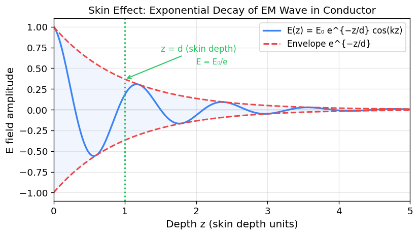
For a conductor with conductivity \(\sigma\), Ampère’s law picks up an extra term: \(\nabla \times \mathbf{B} = \mu(\mathbf{J}_f + \partial_t \mathbf{D}) = \mu(\sigma + i\omega\varepsilon)\mathbf{E}\). The wave vector becomes complex:

\[ \tilde{k}^2 = \mu\varepsilon\omega^2\left(1 + \frac{i\sigma}{\omega\varepsilon}\right). \]

Writing \(\tilde{k} = k + i\kappa\), the wave is \(e^{i(kz-\omega t)}e^{-\kappa z}\): it oscillates but decays exponentially. The skin depth is

\[ d = \frac{1}{\kappa} \approx \sqrt{\frac{2}{\mu\sigma\omega}} \]

(for good conductors where \(\sigma \gg \omega\varepsilon\)). High-frequency fields are excluded from a good conductor — they penetrate only a skin depth before being absorbed. For copper at 60 Hz, \(d \approx 8.5\ \text{mm}\); at 10 GHz, \(d \approx 0.66\ \mu\text{m}\). This is why RF shielding works.

Oblique Incidence: s and p Polarization

The normal-incidence Fresnel equations above are a special case of a richer story. At oblique incidence, the plane containing the wave vector and the surface normal — the plane of incidence — breaks the symmetry between the two transverse polarization directions. Boundary conditions treat these two directions differently, and the reflection and transmission amplitudes depend on which polarization you consider.

s-polarization (from senkrecht, German for perpendicular; also called TE) has \(\mathbf{E}\) perpendicular to the plane of incidence. p-polarization (parallel; also TM) has \(\mathbf{E}\) in the plane of incidence. Any incident wave is a superposition of these two, and they can be handled independently.

Define the auxiliary ratios

\[ \alpha = \frac{\cos\theta_T}{\cos\theta_I} = \frac{\sqrt{1 - (n_1/n_2)^2 \sin^2\theta_I}}{\cos\theta_I}, \qquad \beta = \frac{\mu_1 v_1}{\mu_2 v_2} \approx \frac{n_2}{n_1} \]

where Snell’s law \(n_1\sin\theta_I = n_2\sin\theta_T\) has been used to eliminate \(\theta_T\). The Fresnel equations for s-polarization are:

\[ \frac{\tilde{E}_{R,0}}{\tilde{E}_{I,0}} = \frac{1 - \alpha\beta}{1 + \alpha\beta}, \qquad \frac{\tilde{E}_{T,0}}{\tilde{E}_{I,0}} = \frac{2}{1 + \alpha\beta}. \]

The Fresnel equations for p-polarization are:

\[ \frac{\tilde{E}_{R,0}}{\tilde{E}_{I,0}} = \frac{\alpha - \beta}{\alpha + \beta}, \qquad \frac{\tilde{E}_{T,0}}{\tilde{E}_{I,0}} = \frac{2}{\alpha + \beta}. \]

At normal incidence \(\theta_I = 0\), both cases give \(\alpha = 1\) and reduce to the familiar forms derived earlier. One can verify that \(R + T = 1\) in both cases, as required by energy conservation, where \(T = \alpha\beta|E_{T,0}/E_{I,0}|^2\) for s-polarization and \(T = \beta|E_{T,0}/E_{I,0}|^2\alpha\) for p-polarization.

Brewster’s angle for p-polarization occurs where \(\alpha = \beta\), making the reflected amplitude vanish. For non-magnetic media where \(\mu_1 = \mu_2 = \mu_0\), the condition \(\beta = n_2/n_1\) yields

\[ \theta_B = \arctan\!\left(\frac{n_2}{n_1}\right). \]

Physically, at Brewster’s angle the reflected and transmitted rays are perpendicular to each other: \(\theta_I + \theta_T = 90°\). The oscillating dipoles in the second medium that re-radiate the “reflected” wave cannot radiate along their own axis — so the p-component (whose induced dipoles are aligned with the would-be reflection direction) produces zero reflected intensity. The s-component is unaffected, so the reflected beam at Brewster’s angle is purely s-polarized. This is why glare-reducing polarizing sunglasses work: sunlight reflected off horizontal surfaces is predominantly s-polarized, and the lenses are oriented to block that component.

For s-polarization, no Brewster angle exists in typical non-magnetic media. The condition \(\alpha\beta = 1\) requires \((\mu_2/\mu_1)^2 \neq 1\), which fails when \(\mu_1 \approx \mu_2 \approx \mu_0\). A Brewster angle for s-polarization would require materials with substantially different magnetic permeabilities — unusual at optical frequencies, but achievable in carefully designed metamaterials.

Total internal reflection occurs when light travels from a denser to a rarer medium (\(n_1 > n_2\)) and \(\theta_I\) exceeds the critical angle \(\theta_c = \arcsin(n_2/n_1)\). Beyond this angle, Snell’s law would require \(\sin\theta_T > 1\), which has no real solution: there is no transmitted propagating wave. Instead, the boundary conditions are satisfied by an evanescent wave in medium 2 — a field that decays exponentially away from the interface with no net energy flow. The reflection coefficient becomes complex with \(|R| = 1\): every photon is reflected. Total internal reflection underpins optical fibers (the glass core has higher \(n\) than the cladding), frustrated total internal reflection sensors, and near-field optical microscopy.

Dispersion and the Optical Response of Matter

The refractive index \(n\) is not a fixed property of a material — it depends on frequency. This frequency dependence, dispersion, is responsible for rainbows, chromatic aberration in lenses, and the separation of colors by a prism. Understanding it requires a microscopic model of how the electromagnetic field interacts with bound electrons.

Phase Velocity and Group Velocity

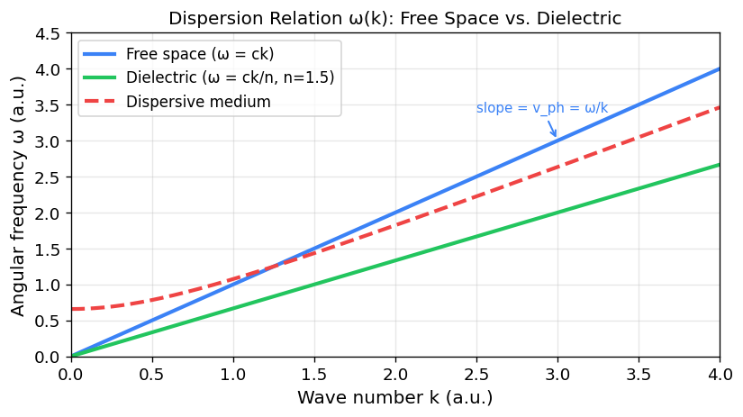
For a monochromatic wave, the phase velocity is the speed at which surfaces of constant phase travel:

\[ v_{\rm ph} = \frac{\omega}{k}. \]

This is \(c/n(\omega)\) in a medium. A wave packet, however, is a superposition of many frequencies, and the group velocity — the speed at which the envelope of the packet propagates — is:

\[ v_g = \frac{\partial\omega}{\partial k}. \]

In vacuum, \(\omega = ck\), so \(v_{\rm ph} = v_g = c\). In a dispersive medium, \(k = n(\omega)\omega/c\), and \(v_{\rm ph} \neq v_g\) in general. The group velocity carries energy and information; the phase velocity can in principle exceed \(c\) near a resonance without violating causality, because the wave packet is distorted and the concept of a well-defined group velocity breaks down in regions of rapid dispersion (anomalous dispersion).

The Lorentz Oscillator Model

A microscopic model treats the electrons in a dielectric as damped driven harmonic oscillators. An electron of mass \(m\) and charge \(q\) bound to an equilibrium position with natural frequency \(\omega_0\) and damping constant \(\gamma\) obeys

\[ m\ddot{x} = -m\omega_0^2 x - m\gamma\dot{x} + qE_0 e^{-i\omega t}. \]

The steady-state solution is \(x(t) = \tilde{x}_0 e^{-i\omega t}\) with

\[ \tilde{x}_0 = \frac{qE_0/m}{\omega_0^2 - \omega^2 - i\gamma\omega}. \]

The induced dipole moment is \(\tilde{p} = q\tilde{x}_0\), and the phase between the driving field and the response depends on frequency:

\[ \delta = \arctan\!\left(\frac{\gamma\omega}{\omega_0^2 - \omega^2}\right). \]

For a medium with \(N\) such oscillators per unit volume, summing over all bound electron transitions (each with oscillator strength \(f_j\), natural frequency \(\omega_j\), and damping \(\gamma_j\)) gives the complex electric susceptibility:

\[ \tilde{\chi}(\omega) = \frac{Nq^2}{m\varepsilon_0}\sum_j \frac{f_j}{\omega_j^2 - \omega^2 - i\gamma_j\omega}. \]

The complex dielectric function is \(\tilde{\varepsilon}(\omega) = \varepsilon_0[1 + \tilde{\chi}(\omega)]\), and the complex wave vector satisfies \(\tilde{k}^2 = \tilde{\varepsilon}\mu_0\omega^2\). Writing \(\tilde{k} = k + i\kappa\), the wave propagates as

\[ \tilde{\mathbf{E}} = \tilde{\mathbf{E}}_0 e^{-\kappa z} e^{i(kz - \omega t)}, \]

so the wave oscillates with wave number \(k = (\omega/c)\,\text{Re}[\tilde{n}]\) and attenuates with absorption coefficient \(\alpha = 2\kappa = 2(\omega/c)\,\text{Im}[\tilde{n}]\). The real part of the complex refractive index determines phase velocity; the imaginary part determines absorption.

Taking the real and imaginary parts of \(\tilde{\chi}\) separately, the real refractive index is approximately

\[ n(\omega) \approx 1 + \frac{Nq^2}{2m\varepsilon_0}\sum_j \frac{f_j(\omega_j^2 - \omega^2)}{(\omega_j^2 - \omega^2)^2 + (\gamma_j\omega)^2}, \]

and the absorption coefficient is

\[ \alpha(\omega) \approx \frac{Nq^2\omega^2}{mc\varepsilon_0}\sum_j \frac{f_j\gamma_j}{(\omega_j^2 - \omega^2)^2 + (\gamma_j\omega)^2}. \]

Far from any resonance (\(\omega \ll \omega_j\) or \(\omega \gg \omega_j\)), the medium is nearly transparent and \(n\) varies slowly — this is the normal dispersion regime where \(dn/d\lambda < 0\) (shorter wavelengths refract more). Near a resonance, \(n\) passes through a maximum, drops steeply, then rises again — the anomalous dispersion region where \(dn/d\lambda > 0\). The absorption is largest at the resonance peak. This behavior is why glass is transparent in the visible but opaque in the UV (electronic resonances) and IR (phonon resonances).

The Plasma Frequency

In the high-frequency limit where \(\omega\) is much larger than all atomic resonances \(\omega_j\), the response simplifies. Every electron in the medium (treating them as essentially free at high frequencies, with \(\omega_0 \to 0\)) contributes equally, and the sum \(\sum_j f_j = Z\) (the total number of electrons per atom) gives:

\[ \tilde{n}^2(\omega) \approx 1 - \frac{NZq^2}{m\varepsilon_0\omega^2} \equiv 1 - \frac{\omega_p^2}{\omega^2}, \]

where the plasma frequency is

\[ \omega_p = \sqrt{\frac{NZq^2}{m\varepsilon_0}}. \]

For \(\omega > \omega_p\), we have \(n^2 > 0\) and the wave propagates normally. For \(\omega < \omega_p\), we have \(n^2 < 0\), meaning \(n\) is purely imaginary: the wave decays exponentially without propagating. The plasma acts as a high-pass filter — electromagnetic waves with frequency below \(\omega_p\) cannot propagate through the medium.

This cutoff is directly observable in the Earth’s ionosphere. The ionosphere is a layer of partially ionized gas at altitudes 60–1000 km with a plasma frequency in the MHz range. AM radio waves (500 kHz to 1600 kHz) are below \(\omega_p\) for the ionosphere and are reflected back to Earth, enabling long-range AM broadcasting. FM radio and television (tens to hundreds of MHz) are typically above the ionospheric \(\omega_p\) and pass straight through, which is why FM cannot be received over the horizon. The same principle governs the reflection of radar by plasmas and the opacity of metals at optical frequencies — the electron density in a metal gives \(\omega_p\) in the UV, so metals reflect visible light (\(\omega < \omega_p\)) but transmit UV (\(\omega > \omega_p\)), a phenomenon confirmed experimentally with thin metal films.

---

Section 2.3: Waveguides and Cavity Resonators

Guided Waves

In a hollow metallic tube — a waveguide — electromagnetic waves are guided along the tube axis by reflections from the conducting walls. For a tube with walls at \(z = \) const, we separate the fields into transverse and longitudinal parts and assume propagation \(e^{i(kz - \omega t)}\). The general solution splits into three mode types:

• TEM modes (transverse electromagnetic): both \(E_z = 0\) and \(B_z = 0\). These exist only in coaxial and two-conductor geometries, not in hollow single-conductor waveguides.
• TE modes (transverse electric): \(E_z = 0\), \(B_z \neq 0\). These are governed by the equation \((\nabla_T^2 + \gamma^2) B_z = 0\) where \(\gamma^2 = (\omega/c)^2 - k^2\).
• TM modes (transverse magnetic): \(B_z = 0\), \(E_z \neq 0\). Similarly governed by \((\nabla_T^2 + \gamma^2) E_z = 0\).

Rectangular Waveguides

For a rectangular guide of dimensions \(a \times b\) (\(a > b\)), the TM modes have:

\[ E_z = E_0 \sin\left(\frac{m\pi x}{a}\right)\sin\left(\frac{n\pi y}{b}\right) e^{i(kz - \omega t)}, \quad m, n = 1, 2, 3, \ldots \]

The TE modes (with \(B_z\) satisfying Neumann boundary conditions):

\[ B_z = B_0 \cos\left(\frac{m\pi x}{a}\right)\cos\left(\frac{n\pi y}{b}\right) e^{i(kz - \omega t)}, \quad m, n = 0, 1, 2, \ldots \]

Each mode \(\text{TE}_{mn}\) or \(\text{TM}_{mn}\) has a cutoff frequency:

\[ \omega_{mn} = c\pi\sqrt{\left(\frac{m}{a}\right)^2 + \left(\frac{n}{b}\right)^2}. \]

Below the cutoff frequency, \(k\) is imaginary and the wave decays exponentially rather than propagating. The dominant mode TE\(_{10}\) has the lowest cutoff \(\omega_{10} = c\pi/a\) and propagates between \(\omega_{10}\) and \(2\omega_{10}\) with only this single mode — useful because it avoids multi-mode dispersion. The phase velocity in the guide is \(v_{\rm ph} = \omega/k > c\), but the group velocity \(v_{\rm gr} = \partial\omega/\partial k = c^2/v_{\rm ph} < c\). No information travels faster than \(c\).

Cavity Resonators

A metallic box with all six walls closed supports standing waves — resonant modes — at discrete frequencies determined by the box dimensions. For a rectangular cavity \(a \times b \times d\):

\[ \omega_{mnl} = c\pi\sqrt{\left(\frac{m}{a}\right)^2 + \left(\frac{n}{b}\right)^2 + \left(\frac{l}{d}\right)^2}. \]

The quality factor \(Q\) measures how many oscillation periods it takes for the stored energy to decay by \(1/e\) due to wall losses: \(Q = \omega_0 U / P_{\rm loss}\), where \(P_{\rm loss}\) arises from finite (but large) conductivity of the walls.

---

Chapter 3: Sources and Radiation

Section 3.1: Potentials and Gauge

Scalar and Vector Potentials

Since \(\nabla \cdot \mathbf{B} = 0\), the magnetic field can always be written as a curl:

\[ \mathbf{B} = \nabla \times \mathbf{A}. \]

Substituting into Faraday’s law gives \(\nabla \times (\mathbf{E} + \partial_t \mathbf{A}) = 0\), so the combination \(\mathbf{E} + \partial_t \mathbf{A}\) is curl-free and can be written as a gradient:

\[ \mathbf{E} = -\nabla V - \partial_t \mathbf{A}. \]

The scalar potential \(V\) and vector potential \(\mathbf{A}\) together carry all the information of the electromagnetic field, and the two remaining Maxwell equations become:

\[ \nabla^2 V + \partial_t (\nabla \cdot \mathbf{A}) = -\frac{\rho}{\varepsilon_0}, \]\[ \left(\nabla^2 \mathbf{A} - \mu_0 \varepsilon_0 \partial_t^2 \mathbf{A}\right) - \nabla\left(\nabla \cdot \mathbf{A} + \mu_0 \varepsilon_0 \partial_t V\right) = -\mu_0 \mathbf{J}. \]

Gauge Freedom

The potentials are not uniquely determined by the fields. A gauge transformation:

\[ \mathbf{A} \to \mathbf{A} + \nabla \Lambda, \qquad V \to V - \partial_t \Lambda \]

leaves \(\mathbf{E}\) and \(\mathbf{B}\) unchanged. We exploit this freedom to simplify the equations.

The Coulomb gauge sets \(\nabla \cdot \mathbf{A} = 0\), giving \(\nabla^2 V = -\rho/\varepsilon_0\) — the instantaneous Poisson equation for \(V\). This is useful for static and quasi-static problems but makes the separation of radiation terms less transparent.

The Lorenz gauge sets

\[ \nabla \cdot \mathbf{A} + \mu_0 \varepsilon_0 \partial_t V = 0, \]

which decouples the wave equations beautifully:

\[ \Box^2 V \equiv \left(\nabla^2 - \mu_0\varepsilon_0 \partial_t^2\right)V = -\frac{\rho}{\varepsilon_0}, \qquad \Box^2 \mathbf{A} = -\mu_0 \mathbf{J}, \]

where \(\Box^2 = \nabla^2 - \frac{1}{c^2}\partial_t^2\) is the d’Alembertian. In the Lorenz gauge, both potentials satisfy the same wave equation driven by their respective sources. This gauge is manifestly Lorentz covariant, a theme we will return to in Part IV.

---

Section 3.2: Retarded Potentials and Moving Charges

Retarded Potentials

The formal solutions of the Lorenz-gauge wave equations are the retarded potentials:

\[ V(\mathbf{r}, t) = \frac{1}{4\pi\varepsilon_0} \int \frac{\rho(\mathbf{r}', t_r)}{\tilde{r}}\, d\tau', \qquad \mathbf{A}(\mathbf{r}, t) = \frac{\mu_0}{4\pi} \int \frac{\mathbf{J}(\mathbf{r}', t_r)}{\tilde{r}}\, d\tau', \]

where \(\tilde{r} = |\mathbf{r} - \mathbf{r}'|\) is the distance from source point \(\mathbf{r}'\) to field point \(\mathbf{r}\), and the retarded time is

\[ t_r = t - \frac{\tilde{r}}{c}. \]

The retarded time embodies causality: the field at \(\mathbf{r}\) at time \(t\) is determined by the source at \(\mathbf{r}'\) at the earlier time \(t_r\), when the signal traveling at speed \(c\) would have left \(\mathbf{r}'\) to arrive at \(\mathbf{r}\) by time \(t\). The advanced potentials (with \(t_r \to t_a = t + \tilde{r}/c\)) are a mathematically valid solution but violate causality.

Jefimenko’s Equations

Taking the appropriate derivatives of the retarded potentials yields the Jefimenko equations — the general retarded solutions for \(\mathbf{E}\) and \(\mathbf{B}\) directly:

\[ \mathbf{E}(\mathbf{r}, t) = \frac{1}{4\pi\varepsilon_0} \int \left[\frac{\rho(\mathbf{r}', t_r)}{\tilde{r}^2}\hat{\tilde{r}} + \frac{\dot{\rho}(\mathbf{r}', t_r)}{c\tilde{r}}\hat{\tilde{r}} - \frac{\dot{\mathbf{J}}(\mathbf{r}', t_r)}{c^2 \tilde{r}}\right] d\tau', \]\[ \mathbf{B}(\mathbf{r}, t) = -\frac{\mu_0}{4\pi} \int \left[\frac{\mathbf{J}(\mathbf{r}', t_r)}{\tilde{r}^2} + \frac{\dot{\mathbf{J}}(\mathbf{r}', t_r)}{c\tilde{r}}\right] \times \hat{\tilde{r}}\, d\tau'. \]

These are the complete, exact, relativistically correct fields for any charge and current distribution. The first terms in \(\mathbf{E}\) and \(\mathbf{B}\) decay as \(1/\tilde{r}^2\) — near-field terms analogous to Coulomb and Biot–Savart but evaluated at the retarded time. The last terms (involving \(\dot{\rho}\) and \(\dot{\mathbf{J}}\)) decay only as \(1/\tilde{r}\) and carry energy to infinity — these are the radiation fields. The naive replacement of the Coulomb law by a retarded version, often stated in textbooks, is an approximation; the \(\dot{\rho}\) and \(\dot{\mathbf{J}}\) terms are not negligible.

Liénard-Wiechert Potentials

For a point charge \(q\) moving on a trajectory \(\mathbf{w}(t)\) with velocity \(\mathbf{v}(t) = \dot{\mathbf{w}}\), evaluating the retarded potentials requires some care: one cannot simply integrate over a delta function distribution naively, because the charge is moving during the time the signal is in flight. The correct result — the Liénard-Wiechert potentials — is obtained by the geometric argument of an information-collecting sphere:

\[ V(\mathbf{r}, t) = \frac{1}{4\pi\varepsilon_0} \frac{qc}{\tilde{r}c - \tilde{\mathbf{r}} \cdot \mathbf{v}} = \frac{q}{4\pi\varepsilon_0} \frac{1}{\tilde{r}(1 - \hat{\tilde{r}} \cdot \mathbf{v}/c)}, \]\[ \mathbf{A}(\mathbf{r}, t) = \frac{\mathbf{v}}{c^2} V(\mathbf{r}, t), \]

where all quantities are evaluated at the retarded position \(\mathbf{w}(t_r)\). The factor \(1 - \hat{\tilde{r}} \cdot \mathbf{v}/c\) in the denominator is a relativistic bunching factor: a charge moving toward you appears stronger because the information-collecting sphere sweeps up more charge per unit time from a source approaching at nearly \(c\). This is the electromagnetic analogue of the Doppler effect, and it leads to the phenomenon of relativistic beaming in synchrotron radiation.

Fields of a Moving Point Charge

The fields derived from the Liénard-Wiechert potentials are:

\[ \mathbf{E}(\mathbf{r}, t) = \frac{q}{4\pi\varepsilon_0} \frac{\tilde{r}}{\left(\tilde{\mathbf{r}} \cdot \mathbf{u}\right)^3} \left[(c^2 - v^2)\mathbf{u} + \tilde{\mathbf{r}} \times (\mathbf{u} \times \dot{\mathbf{v}})\right], \]\[ \mathbf{B}(\mathbf{r}, t) = \frac{1}{c} \hat{\tilde{r}} \times \mathbf{E}(\mathbf{r}, t), \]

where \(\mathbf{u} \equiv c\hat{\tilde{r}} - \mathbf{v}\) and all quantities are evaluated at the retarded time \(t_r\). The first term in \(\mathbf{E}\) (proportional to \(c^2 - v^2\)) is the velocity field or near field: it points from the retarded position in the direction \(\mathbf{u}\), and for a charge at rest reduces to the Coulomb field. The second term (proportional to \(\dot{\mathbf{v}}\), the acceleration) is the radiation field or acceleration field: it falls off as \(1/\tilde{r}\) and carries energy to infinity. A charge in uniform motion produces no radiation; radiation requires acceleration.

---

Section 3.3: Radiation

Radiation from a General Localized Source

Before treating specific geometries, it is worth establishing the general framework. Consider a localized charge distribution — a blob of oscillating charge confined to a region of size \(d\) near the origin. We are interested in the fields far away (\(r \gg d\)) and at wavelengths much larger than the source (\(\lambda/2\pi \gg d\)). These are the radiation zone and long-wavelength approximations respectively.

The starting point is the retarded scalar potential:

\[ V(\mathbf{r}, t) = \frac{1}{4\pi\varepsilon_0}\int \frac{\rho(\mathbf{r}', t_r)}{\tilde{r}}\,d\tau', \qquad t_r = t - \frac{\tilde{r}}{c}. \]

In the far field (\(r \gg r'\)), the separation \(\tilde{r} = |\mathbf{r} - \mathbf{r}'| \approx r - \hat{r}\cdot\mathbf{r}'\), and \(1/\tilde{r} \approx 1/r\). Under these approximations, the potential admits a multipole expansion:

\[ V(\mathbf{r}, t) \approx \frac{1}{4\pi\varepsilon_0}\left[\frac{Q}{r} + \frac{\hat{r}\cdot\mathbf{p}(t_r)}{r^2} + \frac{\hat{r}\cdot\dot{\mathbf{p}}(t_r)}{cr}\right], \]

and the vector potential is simply

\[ \mathbf{A}(\mathbf{r}, t) = \frac{\mu_0}{4\pi}\frac{\dot{\mathbf{p}}(t_r)}{r}, \]

where \(Q = \int\rho\,d\tau\) is the total charge (conserved, so \(\dot{Q} = 0\) produces no radiation), and \(\mathbf{p}(t) = \int\mathbf{r}'\rho(\mathbf{r}', t)\,d\tau'\) is the electric dipole moment.

The key physical point emerges from the structure of these potentials: in the radiation zone (\(r \gg \lambda\)), only the \(1/r\) terms survive when we compute the fields. The term proportional to \(\dot{\mathbf{p}}(t_r)/r\) dominates over the static dipole term \(\mathbf{p}(t_r)/r^2\), and the resulting electric and magnetic fields are:

\[ \mathbf{E}(\mathbf{r}, t) = -\frac{\mu_0}{4\pi r}\ddot{\mathbf{p}}_\perp(t_r), \qquad \mathbf{B}(\mathbf{r}, t) = -\frac{\mu_0}{4\pi rc}\hat{r}\times\ddot{\mathbf{p}}(t_r), \]

where \(\ddot{\mathbf{p}}_\perp = \hat{r}\times(\ddot{\mathbf{p}}\times\hat{r})\) is the component of \(\ddot{\mathbf{p}}\) perpendicular to the line of sight. Note \(\mathbf{E} = -c\hat{r}\times\mathbf{B}\): the radiation fields are transverse to \(\hat{r}\) and mutually perpendicular, propagating outward as a spherical wave.

The time-averaged Poynting vector is

\[ \langle\mathbf{S}\rangle = \frac{\mu_0}{16\pi^2 c}\frac{|\ddot{p}\sin\theta|^2}{r^2}\hat{r}, \]

where \(\theta\) is the angle between \(\hat{r}\) and the dipole axis. Integrating over the full sphere gives the total radiated power:

\[ P = \frac{\mu_0}{6\pi c}\left|\ddot{\mathbf{p}}\right|^2. \]

For a point charge \(q\) with acceleration \(\mathbf{a}\), we have \(\ddot{\mathbf{p}} = q\mathbf{a}\), and this is the Larmor formula:

\[ P = \frac{\mu_0 q^2 a^2}{6\pi c} = \frac{q^2 a^2}{6\pi\varepsilon_0 c^3}. \]

The general formula above contains only the electric dipole term. When the dipole moment vanishes by symmetry (e.g., a centrosymmetric charge distribution), the next term in the multipole expansion — the magnetic dipole moment or the electric quadrupole moment — determines the radiation. These contribute at order \((d/\lambda)^2\) relative to the electric dipole, so they are suppressed by the square of the ratio of source size to wavelength. This hierarchy explains why electric dipole transitions dominate in atomic spectroscopy, with magnetic dipole and electric quadrupole transitions many orders of magnitude weaker.

Electric Dipole Radiation

The simplest radiating system is an oscillating electric dipole: a charge \(q\) oscillating as \(z(t) = z_0 \cos\omega t\), equivalent to a dipole moment \(p(t) = qz_0\cos\omega t\). For a general time-varying dipole \(\mathbf{p}(t)\), the radiation fields at large distances are:

\[ \mathbf{E}_{\rm rad} = \frac{\mu_0}{4\pi r} \left[\ddot{\mathbf{p}}(t_r)\right]_\perp, \qquad \mathbf{B}_{\rm rad} = \frac{1}{c} \hat{r} \times \mathbf{E}_{\rm rad}, \]

where \(\perp\) denotes the component perpendicular to \(\hat{r}\). For the oscillating dipole \(\mathbf{p}(t) = p_0 \cos\omega t\, \hat{z}\), the electric field in the radiation zone is:

\[ \mathbf{E}_{\rm rad} = -\frac{\mu_0 p_0 \omega^2}{4\pi r} \cos\omega(t_r) \sin\theta\, \hat{\theta}, \]

falling off as \(1/r\) and vanishing along the dipole axis (\(\theta = 0\)). The radiation pattern \(\propto \sin^2\theta\) is the characteristic doughnut shape of dipole radiation, with maximum emission perpendicular to the dipole axis and no emission along it.

The time-averaged total radiated power is:

\[ \langle P \rangle = \frac{\mu_0 p_0^2 \omega^4}{12\pi c}. \]

The crucial \(\omega^4\) dependence — Rayleigh’s law — explains why the sky is blue: sunlight scatters off atmospheric molecules, and since blue light has roughly twice the frequency of red light, it scatters \(2^4 = 16\) times more strongly, making the sky appear blue. At sunrise and sunset, when sunlight travels a longer path through the atmosphere, the preferential removal of blue light leaves the red and orange hues of the direct solar disk.

Magnetic Dipole Radiation

A small current loop with magnetic dipole moment \(\mathbf{m}(t) = m_0 \cos\omega t\, \hat{z}\) radiates with exactly the same angular pattern as the electric dipole:

\[ \langle P_{\rm mag} \rangle = \frac{\mu_0 m_0^2 \omega^4}{12\pi c^3}. \]

The ratio of magnetic to electric dipole power for comparable sources scales as \((d\omega/c)^2 \ll 1\), where \(d\) is the physical size of the system. Since \(d\omega/c = d/\lambda\) is the ratio of the system size to the wavelength, magnetic dipole radiation is suppressed relative to electric dipole radiation by a factor of \((d/\lambda)^2\) — typically a very small number at radio and optical frequencies. Magnetic dipole radiation dominates only when electric dipole emission is forbidden by symmetry.

The Larmor Formula

For a point charge \(q\) with acceleration \(\mathbf{a}\), all of the radiation arises from the second term in the Liénard-Wiechert field expression. Integrating the Poynting vector over a sphere at large distances yields the Larmor formula:

\[ P = \frac{\mu_0 q^2 a^2}{6\pi c} = \frac{q^2 a^2}{6\pi \varepsilon_0 c^3}. \]

This result is the foundation of all accelerator physics: any charged particle that is accelerated radiates. A relativistic generalization (the Liénard formula) replaces \(a^2\) with \(\gamma^6[a^2 - |\mathbf{v} \times \mathbf{a}|^2/c^2]\), which for circular motion gives the synchrotron radiation power \(P = \mu_0 q^2 c \gamma^4 / (6\pi R^2)\), growing dramatically with the Lorentz factor \(\gamma\). This is why building high-energy electron accelerators is harder than proton accelerators: electrons, being 1836 times lighter, reach the same \(\gamma\) at much lower energies and radiate much more.

Radiation Reaction

If an accelerating charge radiates energy, Newton’s second law must include a radiation reaction force to account for this energy loss. The self-consistent expression — the Abraham–Lorentz force — is:

\[ \mathbf{F}_{\rm rad} = \frac{\mu_0 q^2}{6\pi c} \dot{\mathbf{a}} = m\tau \dot{\mathbf{a}}, \]

where the characteristic time \(\tau = \mu_0 q^2/(6\pi mc)\). For the electron, \(\tau \approx 6 \times 10^{-24}\ \text{s}\), absurdly smaller than any accessible time scale. The force is proportional to the time derivative of acceleration — a quantity that is poorly constrained by initial conditions — and leads to pathological solutions: runaway acceleration (the charge spontaneously accelerates to infinity with no applied force) and pre-acceleration (the charge starts accelerating before the force is applied). These unphysical solutions are an artifact of treating the electron as a point particle. A proper resolution requires quantum field theory or a finite classical electron radius. The radiation reaction is one of the oldest unresolved problems in classical electrodynamics, and understanding it laid groundwork for renormalization in quantum electrodynamics.

---

Chapter 4: Special Relativity and Covariant Electrodynamics

Section 4.1: Tensors

Rank and Transformation

A tensor is an object defined by how it transforms under coordinate transformations. The rank of a tensor specifies the number of indices required to describe it. A rank-0 tensor is a scalar: it has no indices and is unchanged by rotations or boosts. A rank-1 tensor is a vector: it has one index and transforms as \(A_i' = R_{ij} A_j\) under rotation \(R\). A rank-2 tensor has two indices and transforms as

\[ T_{ij}' = R_{ik} T_{kl} R_{jl}, \]

or in matrix form \(T' = R T R^\top\). Physical examples of rank-2 tensors abound: the moment of inertia tensor \(I_{ij}\), the Cauchy stress tensor \(\sigma_{ij}\) (relating the force per unit area on a surface to its orientation), and the Maxwell stress tensor from Chapter 2.

Index Notation and Einstein Summation

The Einstein summation convention eliminates the need to write summation signs: a repeated index (one upper, one lower) is automatically summed over. For example, the dot product of two vectors is \(A_i B_i \equiv \sum_i A_i B_i\), and the matrix-vector product is \(C_i = M_{ij} B_j \equiv \sum_j M_{ij} B_j\).

The three-dimensional Levi-Civita symbol \(\varepsilon_{ijk}\) takes values \(+1\) for cyclic permutations of \(\{1,2,3\}\), \(-1\) for anticyclic permutations, and \(0\) if any two indices are equal. The curl can be written as \((\nabla \times \mathbf{A})_i = \varepsilon_{ijk} \partial_j A_k\), and the BAC-CAB rule follows from the identity \(\varepsilon_{ijk}\varepsilon_{ilm} = \delta_{jl}\delta_{km} - \delta_{jm}\delta_{kl}\).

The divergence theorem in index notation is \(\int d\tau\, \partial_i v_i = \oint_{\partial\mathcal{V}} da_i v_i\), and Stokes’s theorem is \(\int da_i\, \varepsilon_{ijk} \partial_j v_k = \oint_{\partial\mathcal{S}} dx_i v_i\). These compact forms generalize directly to four dimensions.

---

Section 4.2: Special Relativity

Galilean Relativity and Its Failure

The principle of Galilean relativity — that the laws of physics are the same in all inertial reference frames — seemed secure in Newtonian mechanics. Under a Galilean transformation relating two frames with relative velocity \(v\) along the \(x\)-axis,

\[ t' = t, \quad x' = x - vt, \quad y' = y, \quad z' = z, \]

Newton’s laws are unchanged. But when Maxwell’s equations were discovered, they exhibited a preferred frame: they predicted electromagnetic waves with a fixed speed \(c\), not a relative speed. The natural inference was that this \(c\) was relative to a medium — the luminiferous ether — that filled all space.

The Michelson-Morley experiment (1887) attempted to detect Earth’s motion through the ether by comparing the travel times of light beams sent along and perpendicular to Earth’s velocity. The null result — no detectable phase shift — was profoundly disturbing. Various patch-up attempts (the Lorentz–FitzGerald contraction, Lorentz’s local time) gradually accumulated, but it was Einstein in 1905 who cut through the confusion with a conceptual revolution.

Einstein’s Postulates and Lorentz Transformations

Einstein’s two postulates are:

1. The laws of physics are the same in all inertial reference frames (the principle of relativity).
2. The speed of light in vacuum has the same value \(c\) in all inertial reference frames, regardless of the motion of the source.

Postulate 2 immediately implies the relativity of simultaneity: two events that are simultaneous in one frame are generally not simultaneous in another. This is not a trick or paradox — it reflects that space and time are not absolute but are interwoven into a single entity, spacetime.

From these two postulates and the requirement of linearity (straight worldlines map to straight worldlines), one derives the Lorentz transformation for a boost of velocity \(v\) along the \(x\)-axis:

\[ ct' = \gamma(ct - \beta x), \quad x' = \gamma(x - vt), \quad y' = y, \quad z' = z, \]

where \(\beta = v/c\) and \(\gamma = 1/\sqrt{1 - \beta^2}\) is the Lorentz factor. For \(v \ll c\), \(\gamma \approx 1\) and the Galilean transformation is recovered.

Two immediate consequences:

Time dilation: A clock at rest in the primed frame ticks with period \(\Delta t_0\) (proper time). In the unprimed frame, the same clock appears to tick with period \(\Delta t = \gamma \Delta t_0 > \Delta t_0\). Moving clocks run slow. The proper time satisfies the Lorentz-invariant relation \(c^2 d\tau^2 = c^2 dt^2 - d\mathbf{r}^2\).

Length contraction: A rod of rest length \(\ell_0\) oriented along the direction of motion appears shorter in a frame in which it is moving: \(\ell = \ell_0 / \gamma\). Only the length along the direction of motion is contracted; transverse dimensions are unchanged.

The Lorentz transformation can be elegantly written using the rapidity \(\phi \equiv \tanh^{-1}(v/c)\):

\[ \Lambda = \begin{pmatrix} \cosh\phi & -\sinh\phi \\ -\sinh\phi & \cosh\phi \end{pmatrix} \]

in the \((ct, x)\) subspace. Boosts are therefore hyperbolic rotations in Minkowski spacetime, with rapidity playing the role of angle. Unlike ordinary angles, rapidities add linearly under successive collinear boosts — a great computational convenience.

Minkowski Spacetime and 4-Vectors

Minkowski spacetime is the four-dimensional spacetime with metric

\[ \eta_{\mu\nu} = \text{diag}(+1, -1, -1, -1). \]

The spacetime interval \(s^2 = c^2t^2 - \mathbf{r}^2\) is Lorentz invariant: all inertial observers agree on its value. When \(s^2 > 0\) the interval is timelike (the two events can be causally connected); when \(s^2 < 0\) it is spacelike (no causal connection is possible); when \(s^2 = 0\) it is lightlike (connected by a signal traveling at \(c\)).

A 4-vector \(x^\mu = (ct, \mathbf{r})\) transforms under Lorentz transformations as \(x'^\mu = \Lambda^\mu_{\ \nu} x^\nu\). The covariant (index-down) version \(x_\mu = \eta_{\mu\nu} x^\nu = (ct, -\mathbf{r})\) transforms with the inverse Lorentz matrix. The scalar product \(x \cdot y = x^\mu \eta_{\mu\nu} y^\nu = x^\mu y_\mu\) is Lorentz invariant, generalizing the three-dimensional dot product.

The key 4-vectors in electrodynamics are:

4-vector	Components	Invariant
Position \(x^\mu\)	\((ct, \mathbf{r})\)	\(c^2\tau^2 = c^2t^2 - r^2\)
4-momentum \(p^\mu\)	\((E/c, \mathbf{p})\)	\(m^2c^2 = E^2/c^2 - p^2\)
4-current \(j^\mu\)	\((c\rho, \mathbf{J})\)	(varies)
4-gradient \(\partial^\mu\)	\(\left(\frac{1}{c}\partial_t, -\nabla\right)\)	\(\Box^2 = \frac{1}{c^2}\partial_t^2 - \nabla^2\)

The 4-gradient is covariant (index-down) because it transforms with the inverse Jacobian — the same way basis vectors transform. This is the origin of the minus sign on the spatial components: \(\partial_\mu = \left(\frac{1}{c}\partial_t, +\nabla\right)\) and \(\partial^\mu = \eta^{\mu\nu}\partial_\nu = \left(\frac{1}{c}\partial_t, -\nabla\right)\).

The d’Alembertian in four-dimensional form is the Lorentz-invariant wave operator:

\[ \Box^2 = \partial^\mu \partial_\mu = \frac{1}{c^2}\partial_t^2 - \nabla^2. \]

Local charge conservation \(\partial_t \rho + \nabla \cdot \mathbf{J} = 0\) is simply \(\partial_\mu j^\mu = 0\) — the four-divergence of the 4-current vanishes.

Relativistic Kinematics and Dynamics

The 4-velocity is defined as the derivative of position with respect to proper time:

\[ u^\mu = \frac{dx^\mu}{d\tau} = \gamma(c, \mathbf{v}), \]

and satisfies the Lorentz-invariant normalization \(u^\mu u_\mu = c^2\). The 4-momentum is

\[ p^\mu = mu^\mu = \gamma m (c, \mathbf{v}) = \left(\frac{E}{c},\, \mathbf{p}\right), \]

where \(E = \gamma mc^2\) is the total energy and \(\mathbf{p} = \gamma m\mathbf{v}\) is the relativistic momentum. The Lorentz-invariant mass–energy relation follows immediately:

\[ E^2 = (pc)^2 + (mc^2)^2. \]

For a massless particle like the photon, \(E = pc\). The 4-force is \(F^\mu = dp^\mu/d\tau\), and the work-energy theorem in four dimensions becomes \(F^\mu u_\mu = 0\).

The relativistic generalization of Newton’s second law is:

\[ \frac{d\mathbf{p}}{dt} = q(\mathbf{E} + \mathbf{v} \times \mathbf{B}), \]

where \(\mathbf{p} = \gamma m\mathbf{v}\). Note that the force is the same expression as in classical mechanics — the Lorentz force law is already relativistically correct. What changes is the relation between momentum and velocity.

The twin paradox is resolved geometrically: in Minkowski spacetime, straight worldlines (inertial motion) maximize proper time, just as straight lines minimize length in Euclidean space. The traveling twin, whose worldline is kinked (non-inertial), accumulates less proper time than the stay-at-home twin on the straight worldline. The asymmetry is real and physical, confirmed by atomic clock experiments on aircraft.

---

Section 4.3: Maxwell’s Equations in Covariant Form

The 4-Potential

Maxwell’s equations in the Lorenz gauge take the form \(\Box^2 V = -\rho/\varepsilon_0\) and \(\Box^2 \mathbf{A} = -\mu_0 \mathbf{J}\). Since the source on the right is the 4-current \(j^\mu = (c\rho, \mathbf{J})\), the natural object on the left must be the 4-potential:

\[ A^\mu = \left(\frac{V}{c},\, \mathbf{A}\right). \]

In terms of \(A^\mu\), the Lorenz gauge condition is simply \(\partial_\mu A^\mu = 0\), and the wave equations become the single elegant covariant equation:

\[ \Box^2 A^\mu = -\mu_0 j^\mu. \]

The scalar product \(A \cdot A = (V/c)^2 - A^2\) is Lorentz invariant. The gauge transformation \(A^\mu \to A^\mu + \partial^\mu \Lambda\) leaves the fields invariant; the Lorenz gauge condition selects \(\partial_\mu \partial^\mu \Lambda = 0\).

The Maxwell Field Tensor

The electric and magnetic fields in terms of the potentials are:

\[ \mathbf{B} = \nabla \times \mathbf{A} \implies B_i = \varepsilon_{ijk}\partial_j A_k, \]\[ \mathbf{E} = -\nabla V - \partial_t \mathbf{A} \implies E_i/c = -\partial_i A^0 - \partial^0 A_i. \]

These expressions are precisely the antisymmetric combination \(\partial^\mu A^\nu - \partial^\nu A^\mu\). We define the Maxwell field tensor (or electromagnetic field tensor):

\[ F^{\mu\nu} \equiv \partial^\mu A^\nu - \partial^\nu A^\mu. \]

This is manifestly antisymmetric: \(F^{\mu\nu} = -F^{\nu\mu}\), so the diagonal components vanish and there are only 6 independent components — exactly the 3 components of \(\mathbf{E}\) and 3 of \(\mathbf{B}\). Explicitly:

\[ \left[F^{\mu\nu}\right] = \begin{pmatrix} 0 & E_x/c & E_y/c & E_z/c \\ -E_x/c & 0 & B_z & -B_y \\ -E_y/c & -B_z & 0 & B_x \\ -E_z/c & B_y & -B_x & 0 \end{pmatrix}. \]

The structure has a beautiful geometric interpretation: the electric field components occupy the time–space planes (\(\mu = 0, \nu = i\) or vice versa), while the magnetic field components occupy the space–space planes (\(\mu = i, \nu = j\) both spatial). Under a Lorentz boost, the time–space and space–space planes mix, so electric and magnetic fields mix — they are not separately Lorentz invariant.

Covariance of Maxwell’s Equations

This is the point of the exercise. Maxwell’s four equations collapse into just two tensor equations:

\[ \partial_\nu F^{\mu\nu} = \mu_0 j^\mu \qquad \text{(Gauss's law + Ampère–Maxwell)} \]\[ \partial_\lambda F_{\mu\nu} + \partial_\mu F_{\nu\lambda} + \partial_\nu F_{\lambda\mu} = 0 \qquad \text{(Faraday + no monopoles)} \]

The second equation, the Bianchi identity, is automatically satisfied when \(F_{\mu\nu} = \partial_\mu A_\nu - \partial_\nu A_\mu\). The first encodes both \(\nabla \cdot \mathbf{E} = \rho/\varepsilon_0\) (for \(\mu = 0\)) and \(\nabla \times \mathbf{B} = \mu_0 \mathbf{J} + \mu_0\varepsilon_0 \partial_t \mathbf{E}\) (for \(\mu = i\)). The charge conservation law \(\partial_\mu j^\mu = 0\) follows automatically from the antisymmetry of \(F^{\mu\nu}\): \(\partial_\mu \partial_\nu F^{\mu\nu} = 0\) by symmetry.

Transformation Properties of E and B

Since \(F^{\mu\nu}\) is a rank-2 Lorentz tensor, it transforms under a boost with velocity \(v\) along the \(x\)-axis as:

\[ F'^{\mu\nu} = \Lambda^\mu_{\ \sigma}\, F^{\sigma\tau}\, \Lambda^\nu_{\ \tau}. \]

Working this out explicitly gives the transformation rules for \(\mathbf{E}\) and \(\mathbf{B}\):

\[ E_x' = E_x, \quad E_y' = \gamma(E_y - vB_z), \quad E_z' = \gamma(E_z + vB_y), \]\[ B_x' = B_x, \quad B_y' = \gamma\!\left(B_y + \frac{v}{c^2}E_z\right), \quad B_z' = \gamma\!\left(B_z - \frac{v}{c^2}E_y\right). \]

Components along the boost direction are unchanged; transverse components mix. The critical insight — emphasized by the structure of the field tensor — is that neither \(\mathbf{E}\) nor \(\mathbf{B}\) is Lorentz covariant on its own. Only the combination packaged in \(F^{\mu\nu}\) has this property. An electric field in one frame appears partially as a magnetic field in another, and vice versa.

As a concrete illustration: consider a capacitor at rest with charge density \(\pm\sigma\) producing a field \(E_z = \sigma/\varepsilon\) between the plates and \(\mathbf{B} = 0\). In a frame moving with velocity \(v\) parallel to the plates (along \(\hat{x}\)), the plate length contracts, increasing the charge density to \(\sigma' = \gamma\sigma\). The field tensor transformation gives \(E_z' = \gamma E_z = \gamma\sigma/\varepsilon\) — consistent with the higher charge density. The transformation also produces a magnetic field \(B_y' = -\gamma v E_z/c^2 = -v\sigma'/\varepsilon c^2\), which is exactly what one computes from the surface current \(K' = v\sigma'\) using Ampère’s law. The two approaches agree perfectly, which they must since they are related by a Lorentz transformation of the same underlying field tensor.

The two Lorentz invariants constructible from the field tensor are:

\[ F_{\mu\nu}F^{\mu\nu} = 2\left(B^2 - \frac{E^2}{c^2}\right), \qquad \varepsilon^{\mu\nu\rho\sigma}F_{\mu\nu}F_{\rho\sigma} = \frac{8}{c}\mathbf{E} \cdot \mathbf{B}. \]

The first invariant tells us that if \(E > cB\) in one frame, it is greater in all frames; the second tells us that if \(\mathbf{E} \cdot \mathbf{B} = 0\) in one frame (as for a plane wave), it vanishes in all frames.

---

Appendix: Mathematical Tools

Handy Identities in 3D

\[ \mathbf{A} \times (\mathbf{B} \times \mathbf{C}) = \mathbf{B}(\mathbf{A}\cdot\mathbf{C}) - \mathbf{C}(\mathbf{A}\cdot\mathbf{B}). \]

The Levi-Civita contraction identity: \(\varepsilon_{ijk}\varepsilon_{imn} = \delta_{jm}\delta_{kn} - \delta_{jn}\delta_{km}\).

Green’s identities from the divergence theorem:

\[ \int_\mathcal{V} \left(f\nabla^2 g - g\nabla^2 f\right) d\tau = \oint_{\partial\mathcal{V}} (f\nabla g - g\nabla f)\cdot d\mathbf{a}. \]

Selected Integral Formulas

For the retarded potential calculations, two integrals appear frequently:

\[ \int_{-\infty}^{\infty} \frac{dx}{(x^2 + a^2)^{3/2}} = \frac{2}{a^2}, \qquad \int_{-\infty}^{\infty} \frac{dx}{(x^2 + a^2)^2} = \frac{\pi}{2a^3}. \]

And for Fourier analysis in waveguides:

\[ \int_0^\pi \sin(nx)\sin(mx)\, dx = \int_0^\pi \cos(nx)\cos(mx)\, dx = \frac{\pi}{2}\delta_{n,m}. \]