Motivation

Applied stochastic processes arise whenever a deterministic model is insufficient because of inherent randomness in the system, uncertainty in initial conditions, or noise corrupting observations. Professor Namachchivaya opens the course by surveying five motivating contexts that will recur throughout the semester.

Random walk and the heat equation. A particle performing a simple random walk on the integers — stepping right with probability \(1/2\) and left with probability \(1/2\) — gives rise, in the diffusive limit, to the heat equation \(\partial_t u = \frac{1}{2}\partial_{xx} u\). This passage from discrete randomness to a continuous partial differential equation is the prototype for the entire theory of diffusion processes developed later.

Black–Scholes and financial mathematics. The log-normal model for asset prices, \(dS = \mu S\,dt + \sigma S\,dW\), requires stochastic calculus (AMATH 777) for its full treatment, but the probabilistic foundations — Brownian motion, martingales, conditional expectation — are built in this course.

Sequential decision-making and change-point detection. Many engineering and statistical problems require detecting a change in the distribution of a data stream as quickly as possible while controlling the false-alarm rate. Optimal stopping theory and martingale methods provide the rigorous framework.

Kalman filter and data assimilation. The linear-Gaussian filtering problem — estimating a hidden state \(X_k\) from noisy observations \(Y_k = H_k X_k + V_k\) — is solved exactly by the discrete-time Kalman filter, the culminating topic of the course. In geophysical and meteorological applications, this is called data assimilation: blending model predictions with real observations to produce optimal state estimates.

Gaussian PDF evolution for dynamical systems. For a linear stochastic differential equation \(dX = AX\,dt + B\,dW\), the probability density of the state remains Gaussian for all time, with mean and covariance satisfying tractable ordinary differential equations. This deterministic evolution of uncertainty is at the heart of practical filtering.

The course is organized in five parts: (1) review of probability and random variables; (2) MMSE estimation and projections in \(L^2\); (3) random processes, martingales, and Markov chains; (4) the filtering problem; (5) ODE supplement. The mathematical language throughout is measure-theoretic probability, introduced carefully in the early lectures.

---

Basic Probability — Foundations

Probability Spaces

A \(\sigma\)-algebra \(\mathcal{F}\) satisfies three axioms: (i) \(\Omega \in \mathcal{F}\); (ii) if \(A \in \mathcal{F}\) then \(A^c \in \mathcal{F}\); (iii) if \(A_1, A_2, \ldots \in \mathcal{F}\) then \(\bigcup_{n=1}^\infty A_n \in \mathcal{F}\). The closure under countable unions, combined with complementation, implies closure under countable intersections by De Morgan’s law: \((\bigcup_n A_n)^c = \bigcap_n A_n^c\).

The Kolmogorov axioms for the probability measure are: (i) \(P(A) \ge 0\) for all \(A \in \mathcal{F}\); (ii) \(P(\Omega) = 1\); (iii) countable additivity — if \(A_1, A_2, \ldots\) are pairwise disjoint then \(P(\bigcup_n A_n) = \sum_n P(A_n)\).

From these axioms one derives: \(P(\emptyset) = 0\) (take \(A_n = \emptyset\) for all \(n\) in countable additivity); \(P(A^c) = 1 - P(A)\); the inclusion-exclusion principle \(P(A \cup B) = P(A) + P(B) - P(A \cap B)\); and the monotonicity \(A \subseteq B \Rightarrow P(A) \le P(B)\).

Continuity of Probability

Both results follow from writing the limit set as a disjoint union and applying countable additivity.

---

Random Variables and Distributions

Random Variables

The Borel \(\sigma\)-algebra \(\mathcal{B}(\mathbb{R})\) is the smallest \(\sigma\)-algebra containing all open intervals. It contains all open sets, closed sets, and countable intersections and unions thereof. The real line is uncountable, which motivates the introduction of the Borel structure: we cannot sensibly assign probability to every subset of \(\mathbb{R}\) (the Vitali construction shows this would violate countable additivity), so we restrict to measurable sets.

Discrete examples. A fair coin toss has \(\Omega = \{H, T\}\). Define \(X(H) = 1\), \(X(T) = 0\). Then \(X\) follows the Bernoulli(1/2) distribution. More generally, \(X \sim \text{Bernoulli}(p)\) has \(P(X=1)=p\) and \(P(X=0)=1-p\).

The Geometric distribution models the number of trials until the first success in a sequence of independent Bernoulli trials: \(P(X=k) = (1-p)^{k-1}p\), \(k = 1, 2, \ldots\).

The Poisson distribution models the number of events in a fixed time interval when events occur at constant average rate \(\lambda\): \(P(X=k) = e^{-\lambda}\lambda^k/k!\), \(k = 0, 1, 2, \ldots\)

The Binomial distribution counts successes in \(n\) independent Bernoulli trials: \(P(X=k) = \binom{n}{k}p^k(1-p)^{n-k}\).

---

Distributions, Expectation, and Properties

Cumulative Distribution Function

The CDF has three fundamental properties: (i) monotonicity — \(x \le y \Rightarrow F(x) \le F(y)\); (ii) limits — \(\lim_{x \to -\infty} F(x) = 0\) and \(\lim_{x \to +\infty} F(x) = 1\); (iii) right-continuity — \(\lim_{y \downarrow x} F(y) = F(x)\). These properties follow directly from the continuity of probability and the axioms.

For a continuous random variable, the probability density function (PDF) \(p_X(x)\) satisfies \(F_X(x) = \int_{-\infty}^x p_X(t)\,dt\) and \(p_X(x) \ge 0\), \(\int_{-\infty}^\infty p_X(x)\,dx = 1\).

Expectation

The expectation of a random variable is defined as the Lebesgue integral with respect to the probability measure: \(E[X] = \int_\Omega X(\omega)\,dP(\omega)\). For a discrete random variable, this reduces to \(E[X] = \sum_k k\, P(X=k)\), and for a continuous one, \(E[X] = \int_{-\infty}^\infty x\, p_X(x)\,dx\).

For the binomial distribution \(X \sim \text{Binomial}(n,p)\), \(E[X] = np\). This follows from writing \(X = \sum_{i=1}^n X_i\) where \(X_i\) are i.i.d. Bernoulli, and using linearity of expectation. For the geometric distribution, \(E[X] = 1/p\).

The law of the unconscious statistician states \(E[g(X)] = \int g(x)\,p_X(x)\,dx\) for measurable \(g\), allowing computation of moments without finding the distribution of \(g(X)\) explicitly.

---

Expectation, Moments, and Conditional Probability

Characteristic Functions and Cumulants

The \(n\)-th moment of \(X\) is \(\mu_n = E[X^n]\). The variance is \(\text{Var}(X) = E[(X - E[X])^2] = E[X^2] - (E[X])^2\).

The characteristic function is \(\phi_X(t) = E[e^{itX}]\), which always exists and determines the distribution uniquely. Its series expansion gives moments: \(\phi_X(t) = \sum_{n=0}^\infty \frac{(it)^n}{n!} E[X^n]\). The moment generating function is \(M_X(t) = E[e^{tX}]\), when it exists in a neighborhood of zero.

The cumulant generating function is \(\log M_X(t) = \sum_{n=1}^\infty \kappa_n t^n/n!\). The cumulants \(\kappa_n\) are related to moments: \(\kappa_1 = E[X]\), \(\kappa_2 = \text{Var}(X)\), and higher cumulants measure departure from Gaussianity. For a Gaussian, all cumulants of order \(\ge 3\) are zero.

Key Continuous Distributions

The Exponential distribution with rate \(\lambda > 0\) has PDF \(p(x) = \lambda e^{-\lambda x}\) for \(x \ge 0\). Its mean is \(1/\lambda\) and variance \(1/\lambda^2\).

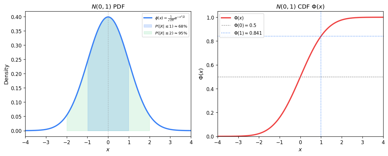
The Gaussian (Normal) distribution \(X \sim N(\mu, \sigma^2)\) has PDF \(p(x) = \frac{1}{\sqrt{2\pi\sigma^2}}\exp\!\left(-\frac{(x-\mu)^2}{2\sigma^2}\right)\). The standard normal \(N(0,1)\) has CDF \(\Phi(u) = \int_{-\infty}^u \frac{1}{\sqrt{2\pi}}e^{-x^2/2}\,dx\) and the complementary function \(Q(u) = 1 - \Phi(u)\). The verification that the Gaussian PDF integrates to one uses the polar-coordinate trick: defining \(I = \int_{-\infty}^\infty e^{-u^2/2}\,du\), squaring to get \(I^2 = \int\!\!\int e^{-(u^2+v^2)/2}\,du\,dv = 2\pi\), so \(I = \sqrt{2\pi}\).

The Cauchy distribution has PDF \(p(x) = \frac{1}{\pi(1+x^2)}\). It is a notable example where the mean does not exist, since the integral \(\int_{-\infty}^\infty |x|/(1+x^2)\,dx\) diverges.

Conditional Probability

This is the rescaled probability restricted to the event \(F\). Conditional probability is itself a probability measure on \((\Omega, \mathcal{F})\) conditioned on \(F\).

---

Conditional Expectation and Bayes’ Law

Bayes’ Theorem and Total Probability

Bayes’ theorem is the engine of Bayesian inference: given prior probabilities \(P(B_i)\) and likelihood \(P(A|B_i)\), the posterior \(P(B_i|A)\) is updated evidence about the state \(B_i\).

Conditional Expectation

For continuous random variables \(X\) and \(Y\) with joint density \(p_{XY}\), the conditional density of \(X\) given \(Y = y\) is \(p_{X|Y}(x|y) = p_{XY}(x,y)/p_Y(y)\), and the conditional expectation is \(E[X|Y=y] = \int x\, p_{X|Y}(x|y)\,dx\).

The abstract definition via \(\sigma\)-algebras is more general and foundational. Given a sub-\(\sigma\)-algebra \(\mathcal{G} \subseteq \mathcal{F}\), the conditional expectation \(E[X|\mathcal{G}]\) is the unique \(\mathcal{G}\)-measurable random variable satisfying the partial averaging property: for every \(G \in \mathcal{G}\),

\[ \int_G E[X|\mathcal{G}]\,dP = \int_G X\,dP. \]

Properties of conditional expectation:

1. Linearity: \(E[aX + bY|\mathcal{G}] = aE[X|\mathcal{G}] + bE[Y|\mathcal{G}]\).
2. Tower property (iterated conditioning): If \(\mathcal{H} \subseteq \mathcal{G}\), then \(E[E[X|\mathcal{G}]|\mathcal{H}] = E[X|\mathcal{H}]\). In particular, \(E[E[X|Y]] = E[X]\).
3. Taking out what is known: If \(Z\) is \(\mathcal{G}\)-measurable, then \(E[ZX|\mathcal{G}] = Z\,E[X|\mathcal{G}]\).
4. Independence: If \(X\) is independent of \(\mathcal{G}\), then \(E[X|\mathcal{G}] = E[X]\).
5. Jensen’s inequality: For convex \(\varphi\), \(\varphi(E[X|\mathcal{G}]) \le E[\varphi(X)|\mathcal{G}]\).

The best approximation property of conditional expectation states that among all \(\mathcal{G}\)-measurable functions \(g\), the function \(E[X|\mathcal{G}]\) minimizes \(E[(X - g)^2]\).

This is the MMSE interpretation: \(E[X|Y]\) is the best predictor of \(X\) given observation \(Y\).

Memoryless Property of the Exponential Distribution

Proof: For \(X \sim \text{Exp}(\lambda)\), \(P(X > x) = e^{-\lambda x}\), so

\[ P(X > s+t|X>s) = \frac{P(X>s+t)}{P(X>s)} = \frac{e^{-\lambda(s+t)}}{e^{-\lambda s}} = e^{-\lambda t} = P(X>t). \]

---

Borel–Cantelli, Convergence Theorems, and Transformations

The Borel–Cantelli Lemmas

The event \(\{A_n \text{ i.o.}\} = \limsup_n A_n = \bigcap_{n=1}^\infty \bigcup_{k=n}^\infty A_k\) reads “infinitely many of the \(A_n\) occur.”

Proof of I: For any \(m\), \(P(A_n \text{ i.o.}) \le P\!\left(\bigcup_{k=m}^\infty A_k\right) \le \sum_{k=m}^\infty P(A_k) \to 0\) as \(m \to \infty\), since the tail of a convergent series vanishes.

Fundamental Convergence Theorems

These three theorems govern when the limit and integral (or expectation) can be interchanged, and are foundational to stochastic analysis.

Transformations of Random Variables

Given a differentiable bijection \(y = g(x)\) with inverse \(x = g^{-1}(y)\), the density of \(Y = g(X)\) is

\[ p_Y(y) = p_X(g^{-1}(y))\left|\frac{d g^{-1}}{dy}\right|. \]

For a multivariate transformation \(\mathbf{Y} = g(\mathbf{X})\) in \(\mathbb{R}^n\), the Jacobian determinant replaces the scalar derivative. The Rayleigh distribution example: if \(X,Y\) are i.i.d. \(N(0,\sigma^2)\), then \(R = \sqrt{X^2+Y^2}\) has the Rayleigh density \(p_R(r) = (r/\sigma^2)e^{-r^2/(2\sigma^2)}\) for \(r \ge 0\).

---

Four Modes of Convergence

Given a sequence of random variables \(X_1, X_2, \ldots\) and a target \(X\), four modes of convergence are defined and studied.

Relationships among modes: (a.s.) \(\Rightarrow\) (p.) \(\Rightarrow\) (d.); (m.s.) \(\Rightarrow\) (p.) \(\Rightarrow\) (d.). Neither (a.s.) nor (m.s.) implies the other in general.

The implication (m.s.) \(\Rightarrow\) (p.) follows from Markov’s inequality: for any \(\varepsilon > 0\),

\[ P(|X_n - X| > \varepsilon) \le \frac{E[(X_n-X)^2]}{\varepsilon^2} \to 0. \]

Chebyshev’s inequality is a special case: \(P(|X - \mu| \ge k\sigma) \le 1/k^2\).

Central Limit Theorem

Heuristic via characteristic functions. Let \(S_n = (X_1+\cdots+X_n - n\mu)/(\sigma\sqrt{n})\). The characteristic function of \(X_i - \mu\) is \(\phi(t) = 1 - \sigma^2 t^2/2 + O(t^3)\). By independence, the characteristic function of \(S_n\) is \(\phi(t/(\sigma\sqrt{n}))^n = (1 - t^2/(2n) + O(n^{-3/2}))^n \to e^{-t^2/2}\), which is the characteristic function of \(N(0,1)\).

---

Lectures 9–11: Minimum Mean-Square Error Estimation

The Geometry of \(L^2\)

The space \(L^2(\Omega,\mathcal{F},P)\) consists of all square-integrable random variables with inner product \((U,V) = E[UV]\) and norm \(\|U\|^2 = E[U^2]\). This is a Hilbert space — complete and having an orthogonality structure that makes projection well-defined.

The projection satisfies: (i) linearity \(\Pi_V(aX+bY) = a\Pi_V X + b\Pi_V Y\); (ii) if \(V_1 \subseteq V_2\) then \(\Pi_{V_1}\Pi_{V_2} = \Pi_{V_1}\); (iii) if \(V_1 \perp V_2\) then \(\Pi_{V_1 \oplus V_2} = \Pi_{V_1} + \Pi_{V_2}\).

Linear MMSE Estimator

Given observations \(Y_1, \ldots, Y_n\), the linear MMSE estimator of \(X\) is the best linear combination \(\hat{X} = \sum_{i=1}^n \alpha_i Y_i\). By the orthogonality principle, the optimal coefficients satisfy \(E[(X - \hat{X})Y_i] = 0\) for all \(i\), yielding the normal equations.

For a single observation \(Y\): \(\hat{X} = E[X] + \text{Cov}(X,Y)\text{Var}(Y)^{-1}(Y - E[Y])\) with estimation error \(\text{Var}(X) - \text{Cov}(X,Y)^2/\text{Var}(Y)\).

Gram–Schmidt and Innovations

The sequence \(\tilde{Y}_k\) consists of the innovations — the new information brought by each observation beyond what was already predictable from prior ones. Since orthogonal variables have a trivial joint projection (sum of individual projections), working with the innovations simplifies the MMSE formula to

\[ \hat{E}[X|Y_1,\ldots,Y_n] = E[X] + \sum_{k=1}^n \frac{\text{Cov}(X,\tilde{Y}_k)}{\text{Var}(\tilde{Y}_k)}\tilde{Y}_k. \]

Vector MMSE and Schur Complements

For random vectors \(X \in \mathbb{R}^n\) and \(Y \in \mathbb{R}^m\), the vector MMSE estimator is

\[ \hat{X} = E[X] + R_{XY}R_Y^{-1}(Y - E[Y]), \]

where \(R_{XY} = \text{Cov}(X,Y)\) and \(R_Y = \text{Cov}(Y,Y)\). The estimation error covariance is

\[ P = R_X - R_{XY}R_Y^{-1}R_{YX}. \]

The derivation uses block Gaussian elimination. Write the joint covariance matrix as a block matrix

\[ \begin{pmatrix} R_X & R_{XY} \\ R_{YX} & R_Y \end{pmatrix}. \]

The Schur complement of the \(R_Y\) block is \(\Delta_A = R_X - R_{XY}R_Y^{-1}R_{YX}\), which equals the minimum achievable error covariance. The block factorization

\[ \begin{pmatrix} I & 0 \\ -R_{YX}R_X^{-1} & I \end{pmatrix}\begin{pmatrix} R_X & R_{XY} \\ R_{YX} & R_Y \end{pmatrix}\begin{pmatrix} I & -R_X^{-1}R_{XY} \\ 0 & I \end{pmatrix} = \begin{pmatrix} R_X & 0 \\ 0 & \Delta_D \end{pmatrix} \]

leads directly to the optimal gain matrix via completing the square in the mean-square error.

Recursive MMSE Estimation

Instead of inverting the full covariance matrix of all past observations when a new observation arrives, one can update the estimate recursively using the innovations. This is the key idea behind the Kalman filter.

Suppose we have the estimate \(\hat{X}_{k-1}\) based on \(Y_1, \ldots, Y_{k-1}\). When the new observation \(Y_k\) arrives, the innovation is

\[ \tilde{Y}_k = Y_k - \hat{E}[Y_k | Y_1, \ldots, Y_{k-1}]. \]

The update takes the form

\[ \hat{X}_k = \hat{X}_{k-1} + B_k \tilde{Y}_k,\quad B_k = \frac{(X, \tilde{Y}_k)_{L^2}}{(\tilde{Y}_k, \tilde{Y}_k)_{L^2}}. \]

For the scalar example with \(X\) unknown constant observed with additive noise \(Y_k = X + V_k\) where \(V_k\) are i.i.d. with variance \(a^2\), the recursive scalar update is:

\[ \hat{X}_k = \hat{X}_{k-1} + \frac{P_{k-1}}{P_{k-1}+a^2}(Y_k - \hat{X}_{k-1}),\quad P_k = \frac{a^2 P_{k-1}}{a^2 + P_{k-1}}. \]

The error variance \(P_k\) decreases monotonically to zero as more observations are accumulated, reflecting the fact that more data about a constant signal eventually pins it down completely.

---

Random Processes — Definitions and Basics

Random Processes

A random process can be viewed in three equivalent ways: (i) as a function of two variables \(X(t,\omega)\); (ii) for each fixed \(\omega\), as a deterministic function \(t \mapsto X(t,\omega)\) called a sample path or realization; (iii) for each fixed \(t\), as a random variable \(\omega \mapsto X(t,\omega)\).

The mean function is \(\mu_X(t) = E[X_t]\). The autocorrelation function is \(R_X(t,s) = E[X_t X_s]\). The autocovariance is \(C_X(t,s) = E[(X_t - \mu_X(t))(X_s - \mu_X(s))] = R_X(t,s) - \mu_X(t)\mu_X(s)\). The finite-dimensional distributions are the joint distributions of \((X_{t_1}, \ldots, X_{t_k})\) for all finite subsets of index times.

A Gaussian process is one where every finite collection \((X_{t_1}, \ldots, X_{t_k})\) is jointly Gaussian. Such a process is entirely specified by its mean function and autocovariance function.

Simple Random Walk and Gambler’s Ruin

The simple random walk is defined by \(S_0 = 0\) and \(S_n = S_{n-1} + \xi_n\) where \(\xi_1, \xi_2, \ldots\) are i.i.d. with \(P(\xi_i = +1) = p\) and \(P(\xi_i = -1) = q = 1-p\).

The Gambler’s ruin problem asks: starting with \(k\) dollars, playing against a casino with total wealth \(N\), what is the probability \(\varphi(k)\) of reaching \(N\) before 0? The first-step analysis gives the recurrence \(\varphi(k) = p\varphi(k+1) + q\varphi(k-1)\) with boundary conditions \(\varphi(0) = 0\), \(\varphi(N) = 1\). The solution for \(p \ne q\) is \(\varphi(k) = (1-(q/p)^k)/(1-(q/p)^N)\); for the fair game \(p = q = 1/2\) it simplifies to \(\varphi(k) = k/N\).

---

Martingales in Discrete Time

Definition and Examples

If the equality is replaced by \(\ge\), the process is a submartingale; if by \(\le\), a supermartingale.

Example 1 (Random walk). For the simple symmetric random walk with \(p = q = 1/2\), \(S_n\) is a martingale. So is \(S_n^2 - n\sigma^2\), the quadratic martingale, since \(E[S_{n+1}^2 - (n+1)\sigma^2|\mathcal{F}_n] = S_n^2 + \sigma^2 - (n+1)\sigma^2 = S_n^2 - n\sigma^2\).

Example 2 (Multiplicative martingale). For i.i.d. positive variables \(\xi_k\) with \(E[\xi_k] = 1\), the product \(M_n = \prod_{k=1}^n \xi_k\) is a martingale. This arises in financial modeling: if \(\xi_k\) is the daily return ratio of an asset, then under the risk-neutral measure \(E[\xi_k] = 1\) and the discounted price process is a martingale.

Maximal Inequalities

Proof of Doob’s inequality. Define the stopping time \(\tau = \min\{k \le n : S_k \ge \lambda\}\) (with \(\tau = \infty\) if no such \(k\) exists). On the event \(A = \{\max_{k\le n} S_k \ge \lambda\}\), we have \(\tau \le n\) and by the submartingale property \(\lambda P(A) \le E[S_n \mathbf{1}_A] \le E[S_n]\).

Stopping Times and Optional Stopping

The optional stopping theorem is used to solve the Gambler’s ruin: applying it to the martingale \(S_n\) at the absorption time gives \(E[S_\tau] = E[S_0] = k\). Since \(S_\tau\) equals \(N\) with probability \(\varphi(k)\) and \(0\) otherwise, we get \(N\varphi(k) + 0\cdot(1-\varphi(k)) = k\), confirming \(\varphi(k) = k/N\) in the fair case.

---

Markov and Wiener Processes

Markov Processes

The future is conditionally independent of the past given the present. The transition density \(p(t,x,s,y)\) gives the density of \(X_t = y\) given \(X_s = x\). The Chapman–Kolmogorov equation expresses the consistency of transition densities over multiple time intervals:

\[ p(t,x,u,z) = \int p(t,x,s,y)\,p(s,y,u,z)\,dy,\quad s \in (t,u). \]

A diffusion process is a Markov process characterized by its drift \(b(\xi, t) = \lim_{\Delta t\to 0} E[X_{t+\Delta t} - X_t | X_t = \xi]/\Delta t\) and diffusion coefficient \(a(\xi,t) = \lim_{\Delta t\to 0} E[(X_{t+\Delta t}-X_t)^2|X_t=\xi]/\Delta t\). The Brownian motion is the fundamental diffusion, with \(b \equiv 0\) and \(a \equiv \sigma^2\).

Wiener Process (Brownian Motion)

Additional properties established in the lectures include: (6) positive definiteness of the correlation function (follows from the variance formula); (7) the Markov property — proved by showing the future increments are independent of \(\sigma\{W_s : s \le t\}\), using the Gaussian structure and independence of increments; (8) the martingale property — \(E[W_t | \mathcal{F}_s] = W_s\) for \(s \le t\), following from independent increments; (9) almost sure continuity of paths; (10) nowhere differentiability and unbounded variation — the quadratic variation \(\sum_k (W_{t_{k+1}} - W_{t_k})^2 \to t\) in probability, establishing that Brownian paths are too irregular for ordinary Riemann–Stieltjes integration.

White noise is defined formally as the derivative \(\xi(t) = \dot{W}(t)\). While not a function in the classical sense, it arises as the limit of \(\xi_\delta(t) = (W_{t+\delta} - W_t)/\delta\). The spectral density of \(\xi_\delta\) converges to a constant (flat spectrum) as \(\delta \to 0\), justifying the name “white” noise. The stochastic integral \(\int_0^t h(t-s)\,dW(s)\) — the formal integral against Brownian motion — is the Itô integral, developed rigorously in AMATH 777.

---

Lectures 15–17: Markov Chains

Finite Discrete-Time Markov Chains

The transition matrix \(P = (p_{ij})\) is stochastic: \(p_{ij} \ge 0\) for all \(i,j\) and \(\sum_j p_{ij} = 1\) for all \(i\). The initial distribution \(\pi_0\) is a row vector with \(\pi_0(i) = P(X_0 = i)\).

The Markov theorem states that the finite-dimensional distributions of the chain are completely determined by \(\pi_0\) and \(P\):

\[ P(X_0=i_0, X_1=i_1, \ldots, X_n=i_n) = \pi_0(i_0)\,p_{i_0 i_1}\,p_{i_1 i_2}\cdots p_{i_{n-1}i_n}. \]

Chapman–Kolmogorov and n-Step Transitions

The \(n\)-step transition probabilities are \(p^{(n)}_{ij} = P(X_{n}=j|X_0=i)\), and the matrix of these probabilities is \(P^n\) (the \(n\)-th matrix power). The Chapman–Kolmogorov equation states:

\[ P^{(n+m)} = P^{(n)}\cdot P^{(m)},\quad \text{i.e.,}\quad p^{(n+m)}_{ij} = \sum_k p^{(n)}_{ik}\, p^{(m)}_{kj}. \]

The distribution at time \(n\) is \(\pi_n = \pi_0 P^n\).

Two-State Chain: Explicit Solution

Consider a two-state chain with states \(\{0,1\}\) and transition matrix \(P = \begin{pmatrix}1-\alpha & \alpha \\ \beta & 1-\beta\end{pmatrix}\). The eigenvalues are 1 and \(1-\alpha-\beta\). Diagonalizing yields the explicit formula:

\[ P(X_n = 0) = \frac{\beta}{\alpha+\beta} + \left(1-\alpha-\beta\right)^n\!\left(\pi_0(0) - \frac{\beta}{\alpha+\beta}\right). \]

As \(n \to \infty\), provided \(|1-\alpha-\beta| < 1\), the chain converges to the stationary distribution \(\pi = (\beta/(\alpha+\beta),\, \alpha/(\alpha+\beta))\).

Stationary Distributions and Classification

For a finite-state chain, a stationary distribution always exists (by Perron–Frobenius theory: the matrix \(P\) has eigenvalue 1 with a non-negative left eigenvector).

State classification. State \(j\) is accessible from \(i\) (written \(i \to j\) if \(p^{(n)}_{ij} > 0\) for some \(n \ge 0\). States \(i\) and \(j\) communicate (\(i \leftrightarrow j\) if \(i \to j\) and \(j \to i\). Communication is an equivalence relation, partitioning the state space into communicating classes.

A communicating class \(C\) is closed if \(p_{ij} = 0\) whenever \(i \in C\) and \(j \notin C\) — once the chain enters \(C\), it never leaves. A single-state closed class is an absorbing state. A chain is irreducible if it has exactly one communicating class.

A state \(i\) is recurrent if the chain returns to \(i\) with probability 1, and transient otherwise. For a finite irreducible chain, all states are recurrent. Among recurrent states, \(i\) is positive recurrent if the expected return time \(E[\tau_i | X_0 = i]\) is finite, and null recurrent if it is infinite. For finite chains, all recurrent states are positive recurrent.

Hitting Times and Strong Markov Property

The hitting time to set \(A\) is \(\tau^A = \min\{n \ge 0 : X_n \in A\}\). The hitting probability from state \(i\) is \(h^A_i = P(\tau^A < \infty | X_0 = i)\). These satisfy the linear system: \(h^A_i = 1\) for \(i \in A\), and \(h^A_i = \sum_j p_{ij} h^A_j\) for \(i \notin A\) (with the minimal non-negative solution).

The Strong Markov Property states that at any stopping time \(\tau\), the process “starts fresh” from state \(X_\tau\), independent of the past.

Time Reversibility

A chain with stationary distribution \(\pi\) is time reversible if the detailed balance equations hold:

\[ \pi_i p_{ij} = \pi_j p_{ji}\quad \text{for all } i,j. \]

The time-reversed chain has transition probabilities \(q_{ij} = \pi_j p_{ji}/\pi_i\). If the chain is reversible, \(q_{ij} = p_{ij}\) — the chain looks the same in both directions of time.

---

Introduction to Random Oscillations

Damped Harmonic Oscillator with Random Forcing

The equation of motion for a randomly forced mechanical oscillator is

\[ \ddot{X} + 2\beta\omega\dot{X} + \omega^2 X = f(t),\quad X(t_0)=x_0,\quad \dot{X}(t_0)=v_0, \]

where \(f(t)\) is a stationary Gaussian forcing process with mean \(\mu_f\) and covariance \(C_{ff}(t-s)\), and \(\beta < 1\) (underdamped). The parameters are: \(\beta = b/(2m\omega)\) (damping ratio) and \(\omega^2 = k/m\) (natural frequency).

By variation of parameters, the general solution is

\[ X(t) = g(t-t_0)x_0 + h(t-t_0)v_0 + \int_{t_0}^t h(t-\tau)f(\tau)\,d\tau, \]

where the homogeneous response functions are

\[ g(t) = e^{-\beta\omega t}\!\left(\cos\omega_d t + \frac{\beta\omega}{\omega_d}\sin\omega_d t\right),\quad h(t) = \frac{e^{-\beta\omega t}}{\omega_d}\sin\omega_d t, \]

with \(\omega_d = \omega\sqrt{1-\beta^2}\) the damped natural frequency.

Since the system is linear, the response \(X(t)\) is Gaussian when the forcing and initial conditions are Gaussian. The mean response is

\[ \mu_X(t) = g(t-t_0)E[x_0] + h(t-t_0)E[v_0] + \frac{\mu_f}{\omega^2}(1-g(t-t_0)). \]

For white noise forcing \(C_{ff}(\tau) = 2\pi\Phi_0\delta(\tau)\) and zero mean, the covariance simplifies. In the stationary regime (taking \(t_0 \to -\infty\), the autocovariance of the response is

\[ C_{XX}(\tau) = \frac{\pi\Phi_0}{2\omega^3\beta}\,e^{-\beta\omega|\tau|}\!\left(\cos\omega_d|\tau| + \frac{\beta\omega}{\omega_d}\sin\omega_d|\tau|\right), \]

and the stationary variance is \(C_{XX}(0) = \pi\Phi_0/(2\omega^3\beta)\). This shows that lighter damping (\(\beta \to 0\) leads to larger variance in the response, as the random energy accumulates without sufficient dissipation.

---

Discrete-Time Dynamical Systems and the Filtering Problem

State-Space Formulation

The filtering problem is set up in state-space form. The unknown signal \(X_k \in \mathbb{R}^n\) evolves according to the state equation

\[ X_{k+1} = A_k X_k + W_k, \]

and is observed through the observation equation

\[ Y_k = H_k X_k + V_k. \]

Here \(W_k\) is process noise with \(E[W_k] = 0\), \(\text{Cov}(W_k) = Q_k\), and \(V_k\) is measurement noise with \(E[V_k] = 0\), \(\text{Cov}(V_k) = R_k\). The initial state has \(E[X_0] = \bar{X}_0\) and \(\text{Cov}(X_0) = P_0\). All noise sources and the initial condition are pairwise uncorrelated.

Taking expectations of the state equation yields the mean propagation

\[ \bar{X}_{k+1} = A_k\bar{X}_k. \]

For the covariance, using the uncorrelatedness of \(X_k\) and \(W_k\):

\[ P_{k+1} = A_k P_k A_k^T + Q_k\quad\text{(Lyapunov Difference Equation).} \]

Similarly, \(\bar{Y}_k = H_k\bar{X}_k\) and \(E[(Y_k - \bar{Y}_k)(Y_k-\bar{Y}_k)^T] = H_k P_k H_k^T + R_k\).

In the Gaussian case with \(W_k \sim N(0,Q_k)\) and \(V_k \sim N(0,R_k)\), the state distribution remains Gaussian for all time: \(X_k \sim N(\bar{X}_k, P_k)\).

---

Lectures 20–21: Discrete Kalman Filter — Derivation

The Two-Step Structure

The Kalman filter operates in two alternating steps at each time \(k\):

1. Information update (measurement update): Given the prior \(\hat{X}_{k|k-1}\) (estimate of \(X_k\) based on observations up to \(k-1\) and the new observation \(Y_k\), compute the posterior \(\hat{X}_{k|k}\).

2. Time update (prediction step): Propagate \(\hat{X}_{k|k}\) forward through the dynamics to obtain the prior \(\hat{X}_{k+1|k}\).

Innovations and Information Update

The key insight is to decompose the information in \(Y_k\) into what is already predictable from \(Y_0, \ldots, Y_{k-1}\) and the genuinely new information. The innovation is

\[ \tilde{Y}_k = Y_k - \hat{E}[Y_k | Y_0,\ldots,Y_{k-1}] = Y_k - H_k\hat{X}_{k|k-1}. \]

Using the state equation \(\tilde{Y}_k = H_k \tilde{X}_{k|k-1} + V_k\) where \(\tilde{X}_{k|k-1} = X_k - \hat{X}_{k|k-1}\) is the prior error.

Applying the orthogonality principle from Chapter 3 to update \(\hat{X}_{k|k}\) using the innovation:

\[ \hat{X}_{k|k} = \hat{X}_{k|k-1} + \Sigma_{k|k-1} H_k^T M_k^{-1} \tilde{Y}_k, \]

where \(M_k = H_k\Sigma_{k|k-1}H_k^T + R_k = \text{Cov}(\tilde{Y}_k)\) is the innovation covariance and \(\Sigma_{k|k-1} = \text{Cov}(X_k - \hat{X}_{k|k-1})\) is the prior error covariance.

The posterior error covariance after the information update is

\[ \Sigma_{k|k} = \Sigma_{k|k-1} - \Sigma_{k|k-1}H_k^T M_k^{-1}H_k\Sigma_{k|k-1}^T. \]

An equivalent form using the matrix inversion lemma is \(\Sigma_{k|k}^{-1} = \Sigma_{k|k-1}^{-1} + H_k^T R_k^{-1} H_k\).

Time Update

After the information update, the time update propagates both the posterior estimate and error covariance through the dynamics. Since \(W_k\) is uncorrelated with all observations \(Y_0, \ldots, Y_k\),

\[ \hat{X}_{k+1|k} = A_k \hat{X}_{k|k},\quad \Sigma_{k+1|k} = A_k \Sigma_{k|k} A_k^T + Q_k. \]

The Kalman Filter Equations (Combined)

Combining the two steps, defining the Kalman gain matrix

\[ K_k = A_k \Sigma_{k|k-1} H_k^T \left(H_k\Sigma_{k|k-1}H_k^T + R_k\right)^{-1}, \]

the full recursion for the prior estimate and prior error covariance is:

\[ \hat{X}_{k+1|k} = A_k\hat{X}_{k|k-1} + K_k\left(Y_k - H_k\hat{X}_{k|k-1}\right), \]\[ \Sigma_{k+1|k} = A_k\Sigma_{k|k-1} A_k^T - A_k\Sigma_{k|k-1}H_k^T\left(H_k\Sigma_{k|k-1}H_k^T+R_k\right)^{-1}H_k\Sigma_{k|k-1}A_k^T + Q_k, \]

initialized with \(\hat{X}_{0|-1} = \bar{X}_0\) and \(\Sigma_{0|-1} = P_0\).

The structure of the Kalman filter update \(\hat{X}_{k+1|k} = A_k\hat{X}_{k|k-1} + K_k\tilde{Y}_k\) is a linear dynamical system driven by the innovation sequence. The Kalman gain weights the innovation by the prior uncertainty relative to the observation noise.

---

Lectures 22–23: Kalman Filter — Bayesian Perspective

Filtering as Bayesian Inference

From the probabilistic viewpoint, filtering is about tracking the conditional distribution of the state given all past observations. Define the posterior distribution at time \(k\) as \(\pi_k^u \sim (X_k | Y_0^k)\) and the prior distribution as \(\pi_k^p \sim (X_k | Y_0^{k-1})\).

The two steps of the filter correspond to:

Propagation step: \(\pi_{k-1}^u \to \pi_k^p\) via the Markov transition kernel.

Update step (Bayes’ formula): \(\pi_k^u(dx_k) \propto l(x_k|y_k)\,\pi_k^p(dx_k)\), where \(l(x_k|y_k)\) is the likelihood of the observation.

Gaussian Case: Exact Bayes Update

For the linear-Gaussian model, if the prior at time \(k\) is Gaussian \(\pi_k^p \sim N(X_k^p, P_k^p)\), then after the Bayes update with observation \(Y_k\), the posterior is also Gaussian \(\pi_k^u \sim N(X_k^u, P_k^u)\) with:

\[ X_k^u = X_k^p + P_k^u H_k^T R_k^{-1}(Y_k - H_k X_k^p), \]\[ (P_k^u)^{-1} = (P_k^p)^{-1} + H_k^T R_k^{-1} H_k. \]

The explicit density computation — completing the square in the product of prior and likelihood Gaussians — shows that the posterior is itself Gaussian, confirming that the Gaussian family is closed under Bayesian updating for linear-Gaussian models.

This theorem justifies the Kalman filter as the globally optimal (not just optimal among linear) estimator when all noise is Gaussian. The proof uses the fact that for jointly Gaussian \(X\) and \(Y\), the MMSE error \(\varepsilon = X - \hat{E}[X|Y]\) is independent of \(Y\) (since it is Gaussian and uncorrelated with \(Y\), hence the conditional distribution of \(X\) given \(Y = y\) is \(N(\hat{E}[X|Y=y], \text{Cov}(\varepsilon))\), and so \(E[X|Y=y] = \hat{E}[X|Y=y]\).

Continuous-Time Kalman–Bucy Filter

Passing to the continuous-time limit as the time step \(\Delta t \to 0\) in the scalar model, one obtains the Kalman–Bucy filter. For the model

\[ dX(t) = aX(t)\,dt + b\,dW(t),\quad dY(t) = hX(t)\,dt + g\,dV(t), \]

the filter equations for the conditional mean \(m(t) = E[X(t)|Y_s,\,s \le t]\) and conditional variance \(\gamma(t)\) are:

\[ dm(t) = am(t)\,dt + \frac{h\gamma(t)}{g^2}\left(dY(t) - hm(t)\,dt\right), \]\[ \dot{\gamma}(t) = 2a\gamma(t) + b^2 - \frac{h^2\gamma^2(t)}{g^2}. \]

The second equation is a Riccati equation for the error variance. In the vector case, for the model \(dX = AX\,dt + B\,dW\), \(dY = HX\,dt + G\,dV\), the Kalman–Bucy filter is:

\[ d\pi_t = A\pi_t\,dt + \Sigma_t H^*(GG^*)^{-1}(dY_t - H\pi_t\,dt), \]\[ \dot{\Sigma}_t = A\Sigma_t + \Sigma_t A^* + BB^* - \Sigma_t H^*(GG^*)^{-1}H\Sigma_t, \]

where \(\Sigma_t = E[(X_t - \pi_t)(X_t-\pi_t)^*]\) is the error covariance. The quantity \(d\nu_t = dY_t - H\pi_t\,dt\) is the innovation process in continuous time.

---

Review and Synthesis

MMSE vs. Conditional Expectation

The course distinguishes two estimators whose relationship is a recurring theme. The MMSE linear estimator \(\hat{E}[X|Y]\) is the best estimator restricted to linear functions of \(Y\) and is determined entirely by first and second moments. The conditional mean \(E[X|Y]\) is the best unconstrained estimator (possibly nonlinear).

In general, \(E[(X-E[X|Y])^2] \le E[(X-\hat{E}[X|Y])^2] \le \text{Var}(X)\), with the left inequality being the improvement from using the conditional mean over the linear estimator. When \(X\) and \(Y\) are jointly Gaussian, the two coincide — a fact fundamental to the Kalman filter’s optimality.

Key Examination Topics

The following topics form the core of the course:

Probability and conditional expectations: jointly normal random variables, independence, properties of conditional expectation, Bayes’ theorem.

Stochastic processes: Brownian motion, its properties (Gaussian, zero mean, covariance \(\min(t,s)\), independent increments, Markov, martingale, continuous paths), martingales in discrete time.

Linear stochastic systems: propagation of mean and covariance; Lyapunov equation; first-order ODE review.

Markov chains: communicating classes; invariant distributions; recurrence and transience; long-run behavior.

Estimation: orthogonality principle; conditional expectation as projection; time update and information update steps; discrete-time Kalman filter.

---

ODE Supplement: First-Order Ordinary Differential Equations

Linear First-Order ODEs

The general first-order linear ODE in standard form is

\[ \frac{dy}{dx} + P(x)y = Q(x). \]

Solution by integrating factor. The integrating factor is \(\mu(x) = e^{\int P(x)\,dx}\). Multiplying through converts the left side to an exact differential:

\[ \frac{d}{dx}[\mu(x)y(x)] = \mu(x)Q(x). \]

Integrating and solving for \(y\):

\[ y(x) = e^{-\int P(x)\,dx}\left(c + \int Q(x)\,e^{\int P(x)\,dx}\,dx\right). \]

Solution by variation of parameters. The homogeneous solution is \(y_h = c\varphi(x)\) where \(\varphi(x) = e^{-\int P(x)\,dx}\). The particular solution is sought in the form \(y_p = v(x)\varphi(x)\), leading to \(v'(x) = Q(x)/\varphi(x)\), which recovers the same formula.

Bernoulli Equations

The Bernoulli equation \(\frac{dy}{dx} + P(x)y = Q(x)y^\alpha\) for \(\alpha \ne 0,1\) is nonlinear but reducible to linear form via the substitution \(v = y^{1-\alpha}\):

\[ \frac{dv}{dx} + (1-\alpha)P(x)v = (1-\alpha)Q(x). \]

Riccati Equations

The Riccati equation \(\frac{dy}{dx} = P(x) + Q(x)y + R(x)y^2\) is not generally solvable in closed form. However, if a particular solution \(y_1(x)\) is known, the substitution \(y = y_1 + v\) reduces the equation to a Bernoulli equation for \(v\):

\[ \frac{dv}{dx} - [Q(x) + 2R(x)y_1(x)]v = R(x)v^2. \]

This Bernoulli equation with \(\alpha = 2\) is then solved via \(w = v^{-1}\), yielding a linear ODE for \(w\).

The Riccati structure appears throughout the course: the discrete-time Kalman filter’s error covariance satisfies a matrix Riccati recursion, and the continuous-time error covariance satisfies the matrix Riccati ODE \(\dot{\Sigma} = A\Sigma + \Sigma A^* + BB^* - \Sigma H^*(GG^*)^{-1}H\Sigma\).

---

Tutorial Supplement

Tutorial 2: Linear Scaling and Gaussian Distribution

The linear scaling rule for PDFs states: if \(Y = aX + b\) with \(a > 0\), then \(p_Y(y) = \frac{1}{a}p_X\!\left(\frac{y-b}{a}\right)\). This follows from differentiating the CDF \(F_Y(y) = F_X((y-b)/a)\).

The standard normal integral \(\int_{-\infty}^\infty e^{-x^2/2}\,dx = \sqrt{2\pi}\) is computed via the polar-coordinate trick. For \(X \sim N(\mu,\sigma^2)\), standardization gives \(Y = (X-\mu)/\sigma \sim N(0,1)\), allowing all normal probabilities to be computed from the standard tables.

Tutorial 3: Conditional Expectation

The law of iterated expectations \(E[X] = E[E[X|Y]]\) is fundamental. For discrete \(Y\), it reads \(E[X] = \sum_y E[X|Y=y]P(Y=y)\). The proof follows by expanding the right-hand side and rearranging the double sum. For jointly continuous \((X,Y)\), conditional expectations are computed from the conditional density \(f_{X|Y}(x|y) = f_{XY}(x,y)/f_Y(y)\).

Tutorial 4: MCT and Transformations

A key example illustrating the necessity of the monotonicity assumption in the MCT: the sequence \(f_n = n\mathbf{1}_{(0,1/n]}\) satisfies \(\int f_n = 1\) for all \(n\) but \(f_n \to 0\) pointwise, so \(\lim \int f_n \ne \int \lim f_n\). The sequence is not monotone decreasing, illustrating that MCT requires non-negative monotone sequences.

For the transformation \(Y_1 = 2X_1\), \(Y_2 = X_2 - X_1\) applied to exponential \((X_1, X_2)\), computing the Jacobian (determinant 1/2) and applying the change-of-variables formula yields \(g(y_1, y_2) = e^{-y_1}e^{-y_2}\), proving independence.

Tutorial 5: MMSE Properties

The MMSE estimator is unbiased: \(E[\hat{X}_M] = E[E[X|Y]] = E[X]\) by the tower property. The error is orthogonal to any function of \(Y\): \(E[\tilde{X}\cdot g(Y)] = 0\) for all \(g\). Variance decomposition: \(\text{Var}(X) = \text{Var}(\hat{X}_M) + \text{Var}(\tilde{X})\), since \(\text{Cov}(\tilde{X},\hat{X}_M) = 0\).

Example: \(X \sim N(0,1)\), \(Y = X + W\) with \(W \sim N(0,1)\) independent. Since \(\text{Cov}(X,Y) = 1\) and \(\text{Var}(Y) = 2\), the MMSE estimator is \(\hat{X}_M = Y/2\) with MSE 1/2.

Tutorial 6: Brownian Motion Properties

The covariance function \(\text{Cov}(W_s, W_t) = \min(s,t)\) follows from the independent increments property and the fact that \(W_s = W_s - W_0\) and \(W_t - W_s\) are independent for \(s \le t\).

For the geometric Brownian motion \(X(t) = e^{W(t)}\): using the MGF of the normal, \(E[X(t)] = e^{t/2}\), \(\text{Var}(X(t)) = e^{2t} - e^t\), and for \(s \le t\), \(\text{Cov}(X(s),X(t)) = e^{(3s+t)/2} - e^{(s+t)/2}\).

Tutorial 7: Markov Chain State Distributions

The state distribution at time \(n\) is \(\pi(n) = \pi(0)P^n\). For the two-state example with transition matrix \(P = \begin{pmatrix}1/2&1/2\\1/3&2/3\end{pmatrix}\) and \(\pi(0) = [1,0]\), the probability of being in state 1 at time 3 is computed as the (0,1) entry of \(\pi(0)P^3\), yielding \(43/72\).

Tutorial 8: Kalman Filter Examples

Example 1 (i.i.d. observations of a constant): \(X_k = X_{k-1}\), \(Y_k = X_k + V_k\) with \(V_k \sim N(0,\sigma^2)\). The posterior variance satisfies \(\Sigma_{k|k} = \Sigma_{k-1|k-1}\sigma^2/(\Sigma_{k-1|k-1}+\sigma^2)\), which decreases monotonically. Equivalently, \(\sigma^2/\Sigma_{k|k} = 1 + \sigma^2/\Sigma_{k-1|k-1}\), showing \(\Sigma_{k|k} \to 0\) as \(k \to \infty\).

Example 2 (AR(1) signal): \(X_n = aX_{n-1} + W_n\), \(Y_n = X_n + V_n\). The posterior is \(N(m_n, s_n^2)\) with

\[ m_n = \frac{\tau^2 a m_{n-1} + (a^2 s_{n-1}^2 + \sigma^2)Y_n}{\tau^2 + a^2 s_{n-1}^2 + \sigma^2},\quad s_n^2 = \frac{\tau^2(a^2 s_{n-1}^2 + \sigma^2)}{\tau^2 + a^2 s_{n-1}^2 + \sigma^2}. \]

Simulation with \(a = 0.98\) and unit noise variances shows the filter track closely following the true signal, with the error variance quickly reaching steady state.

---

Expanded Treatment: Probability Theory

Measure Theory Foundations

The development of probability theory on a firm mathematical foundation requires understanding why the measure-theoretic approach is necessary. The naive approach of assigning probabilities to all subsets of a sample space fails for uncountable spaces: the Vitali theorem shows that no translation-invariant measure can be defined on all subsets of \([0,1]\) satisfying countable additivity. The Borel \(\sigma\)-algebra sidesteps this by restricting to the “measurable” subsets.

Generating a \(\sigma\)-algebra. Given a collection of sets \(\mathcal{C}\), the \(\sigma\)-algebra generated by \(\mathcal{C}\), written \(\sigma(\mathcal{C})\), is the smallest \(\sigma\)-algebra containing \(\mathcal{C}\). It exists because the intersection of any collection of \(\sigma\)-algebras is again a \(\sigma\)-algebra. The Borel \(\sigma\)-algebra on \(\mathbb{R}\) is \(\mathcal{B}(\mathbb{R}) = \sigma\{\text{open intervals}\}\).

It is an important fact that \(\mathcal{B}(\mathbb{R})\) can also be generated by any of the following: all open sets; all closed sets; all intervals \((-\infty, x]\) for \(x \in \mathbb{R}\); or all intervals \([a,b)\). This multiplicity of generators is important for characterizing random variables: the condition \(\{X \le x\} \in \mathcal{F}\) for all \(x\) is equivalent to \(X\) being measurable.

Probability measure construction. For a probability model to be self-consistent, we need to know that a probability measure can be built from a specification of finite-dimensional distributions. The Carathéodory extension theorem guarantees that a countably additive set function defined on an algebra extends uniquely to the generated \(\sigma\)-algebra. For stochastic processes, Kolmogorov’s extension theorem provides the corresponding result: a consistent family of finite-dimensional distributions (satisfying symmetry and compatibility conditions) defines a unique measure on the product space.

The Inclusion-Exclusion Principle

For three events \(A, B, C\), the inclusion-exclusion principle generalizes to

\[ P(A \cup B \cup C) = P(A) + P(B) + P(C) - P(A \cap B) - P(A \cap C) - P(B \cap C) + P(A \cap B \cap C). \]

For \(n\) events it reads \(P\!\left(\bigcup_{i=1}^n A_i\right) = \sum_k (-1)^{k+1}\sum_{|S|=k} P\!\left(\bigcap_{i \in S} A_i\right)\). A useful consequence is the union bound (Boole’s inequality): \(P(\bigcup_i A_i) \le \sum_i P(A_i)\).

Detailed Study of the Borel–Cantelli Lemmas

The first Borel–Cantelli lemma, \(\sum_n P(A_n) < \infty \Rightarrow P(\limsup_n A_n) = 0\), is used throughout the course in convergence proofs. The second Borel–Cantelli lemma, \(\sum_n P(A_n) = \infty\) and \(A_n\) independent \(\Rightarrow P(\limsup_n A_n) = 1\), establishes the converse under independence. Note the independence requirement: the lemma fails without it (consider \(A_n = A\) for a single event with \(P(A) = 1/2\); then \(\sum P(A_n) = \infty\) but \(P(A_n \text{ i.o.}) = 1/2 < 1\).

Proof of Borel–Cantelli II. It suffices to show \(P\!\left(\bigcap_{n=1}^\infty \bigcup_{k=n}^\infty A_k\right) = 1\), or equivalently \(P\!\left(\bigcup_{n=1}^\infty \bigcap_{k=n}^\infty A_k^c\right) = 0\). For any fixed \(n\), by independence:

\[ P\!\left(\bigcap_{k=n}^{n+m} A_k^c\right) = \prod_{k=n}^{n+m}(1 - P(A_k)) \le \prod_{k=n}^{n+m} e^{-P(A_k)} = \exp\!\left(-\sum_{k=n}^{n+m}P(A_k)\right) \to 0 \]

as \(m \to \infty\) since \(\sum_k P(A_k) = \infty\). Taking \(m \to \infty\) and applying continuity from above gives \(P(\bigcap_{k=n}^\infty A_k^c) = 0\) for every \(n\), hence the event \(\bigcup_n \bigcap_{k \ge n} A_k^c\) has probability zero.

Random Variables: Deeper Properties

Independence of random variables. Random variables \(X_1, \ldots, X_n\) are independent if the events \(\{X_1 \in B_1\}, \ldots, \{X_n \in B_n\}\) are independent for all Borel sets \(B_i\). Equivalently, the joint CDF factors: \(F_{X_1,\ldots,X_n}(x_1,\ldots,x_n) = \prod_i F_{X_i}(x_i)\). For jointly continuous random variables, independence is equivalent to the joint density factoring as \(p_{X_1,\ldots,X_n}(x_1,\ldots,x_n) = \prod_i p_{X_i}(x_i)\).

Functions of random variables. The distribution function method and the transformation method provide systematic ways to find the distribution of \(Y = g(X)\). For example, if \(X \sim \text{Exp}(\lambda)\) and \(Y = X^2\), then \(P(Y \le y) = P(X \le \sqrt{y}) = 1 - e^{-\lambda\sqrt{y}}\) for \(y \ge 0\), so \(p_Y(y) = \frac{\lambda}{2\sqrt{y}}e^{-\lambda\sqrt{y}}\).

Moment Generating Functions and Cumulants

The moment generating function (MGF) of \(X\) is \(M_X(t) = E[e^{tX}]\). When it exists in a neighborhood of zero, all moments are finite and \(E[X^n] = M_X^{(n)}(0)\). The MGF uniquely determines the distribution (when it exists).

For the normal distribution \(X \sim N(\mu, \sigma^2)\):

\[ M_X(t) = \exp\!\left(\mu t + \frac{\sigma^2 t^2}{2}\right). \]

For the Poisson distribution with rate \(\lambda\): \(M_X(t) = \exp(\lambda(e^t - 1))\).

The cumulant generating function is \(K_X(t) = \log M_X(t)\). The first few cumulants are:

\[ \kappa_1 = K_X'(0) = E[X] = \mu,\quad \kappa_2 = K_X''(0) = \text{Var}(X) = \sigma^2, \]\[ \kappa_3 = K_X'''(0) = E[(X-\mu)^3]\quad\text{(skewness numerator)},\quad \kappa_4 = K_X^{(4)}(0) = \mu_4 - 3\sigma^4\quad\text{(excess kurtosis numerator)}. \]

For the normal distribution, all cumulants of order \(\ge 3\) vanish: \(\kappa_n = 0\) for \(n \ge 3\). This makes the normal distribution uniquely simple from the cumulant perspective and explains why the CLT converges to it.

The moment-cumulant relation expresses moments in terms of cumulants: \(\mu_n' = \sum_{\pi \in \Pi_n} \prod_{B \in \pi} \kappa_{|B|}\), summing over all set partitions of \(\{1,\ldots,n\}\). For example, \(E[X^4] = \kappa_4 + 4\kappa_3\kappa_1 + 3\kappa_2^2 + 6\kappa_2\kappa_1^2 + \kappa_1^4\).

The Exponential Distribution in Detail

The exponential distribution \(\text{Exp}(\lambda)\) is the continuous analogue of the geometric distribution. Its CDF is \(F(x) = 1 - e^{-\lambda x}\) for \(x \ge 0\). The key properties:

• Mean: \(E[X] = 1/\lambda\), computed as \(\int_0^\infty x\lambda e^{-\lambda x}\,dx = 1/\lambda\) by integration by parts.
• Variance: \(\text{Var}(X) = 1/\lambda^2\).
• MGF: \(M_X(t) = \lambda/(\lambda - t)\) for \(t < \lambda\).
• The memoryless property: already proved in Lecture 6; it is the defining characteristic of the exponential among continuous distributions.

The Poisson process and exponential distribution are intimately connected: if events arrive as a Poisson process with rate \(\lambda\), the inter-arrival times are i.i.d. \(\text{Exp}(\lambda)\).

Conditional Expectation: Complete Development

The abstract definition of conditional expectation is motivated by seeking a random variable \(Z = E[X|\mathcal{G}]\) that encodes the best prediction of \(X\) given the information in \(\mathcal{G}\). By the Radon–Nikodym theorem, this exists and is unique: for any \(X \in L^1(\Omega,\mathcal{F},P)\) and sub-\(\sigma\)-algebra \(\mathcal{G}\), there exists a unique (a.s.) \(\mathcal{G}\)-measurable \(Z\) with \(E[Z] = E[X]\) and \(\int_G Z\,dP = \int_G X\,dP\) for all \(G \in \mathcal{G}\).

A detailed verification of the tower property: suppose \(\mathcal{H} \subseteq \mathcal{G}\). We must show \(E[E[X|\mathcal{G}]|\mathcal{H}] = E[X|\mathcal{H}]\), i.e., for every \(H \in \mathcal{H}\),

\[ \int_H E[E[X|\mathcal{G}]|\mathcal{H}]\,dP = \int_H X\,dP. \]

But since \(H \in \mathcal{H} \subseteq \mathcal{G}\), the partial averaging property of the outer conditional expectation gives

\[ \int_H E[E[X|\mathcal{G}]|\mathcal{H}]\,dP = \int_H E[X|\mathcal{G}]\,dP = \int_H X\,dP, \]

where the last equality uses the partial averaging property of \(E[X|\mathcal{G}]\) with \(H \in \mathcal{G}\). Since the characterization holds for all \(H \in \mathcal{H}\), the tower property is established.

The property “taking out what is known”: if \(Z\) is \(\mathcal{G}\)-measurable and bounded, then \(E[ZX|\mathcal{G}] = Z E[X|\mathcal{G}]\). Proof: for any \(G \in \mathcal{G}\),

\[ \int_G Z E[X|\mathcal{G}]\,dP = \int_G ZX\,dP \]

holds by the integral version of the result for indicator functions, extended to general bounded \(Z\) by linearity and monotone convergence.

---

Expanded Treatment: Random Processes

Stationary Processes and Spectral Theory

A random process \(\{X_t\}\) is strictly stationary if its finite-dimensional distributions are invariant under time shifts. It is wide-sense stationary (WSS) or weakly stationary if \(\mu_X(t) = \mu\) (constant) and \(R_X(t,s) = R_X(t-s)\) (depends only on the lag). WSS processes have a rich spectral theory.

The power spectral density (PSD) of a WSS process is the Fourier transform of the autocorrelation:

\[ S_X(\omega) = \int_{-\infty}^\infty R_X(\tau) e^{-i2\pi\omega\tau}\,d\tau. \]

The PSD is real, non-negative, and even. The Wiener–Khinchin theorem states that for a WSS process, \(S_X(\omega)\) is the PSD in the sense that \(\text{Var}(X_t) = R_X(0) = \int_{-\infty}^\infty S_X(\omega)\,d\omega\).

White noise has a flat PSD: \(S_\xi(\omega) \equiv 1\) (or a constant). This is the origin of the term “white” — analogous to white light containing all frequencies equally. The autocovariance of white noise is \(C_\xi(\tau) = \delta(\tau)\). The response of a linear system with transfer function \(H(\omega)\) to white noise has PSD \(S_Y(\omega) = |H(\omega)|^2 S_\xi(\omega) = |H(\omega)|^2\).

For the damped oscillator driven by white noise, the transfer function is

\[ H(\omega) = \frac{1}{\omega_0^2 - \omega^2 + 2i\beta\omega_0\omega}, \]

and the PSD of the response is \(S_X(\omega) = |H(\omega)|^2\), peaked near \(\omega \approx \omega_d\) — the resonance frequency.

Independent Increment Processes

A process \(\{X_t\}\) has independent increments if for all \(t_0 < t_1 < \cdots < t_n\), the increments \(X_{t_1}-X_{t_0}, X_{t_2}-X_{t_1}, \ldots, X_{t_n}-X_{t_{n-1}}\) are independent. This is a special case of the Markov property: knowing the increment structure means past increments carry no additional information about future ones beyond what is encoded in the current position.

The Brownian motion is the most important example. Its increments are not only independent but also stationary (the distribution of \(W_{t+s} - W_t\) depends only on \(s\). Gaussian independent increments with continuous paths and \(\text{Var}(W_t) = \sigma^2 t\) characterize Brownian motion uniquely.

---

Expanded Treatment: Martingales

Filtrations and Natural Filtrations

A filtration \((\mathcal{F}_n)_{n \ge 0}\) is an increasing sequence of \(\sigma\)-algebras: \(\mathcal{F}_0 \subseteq \mathcal{F}_1 \subseteq \cdots \subseteq \mathcal{F}\). The filtration models the accumulation of information over time. The natural filtration of a process \(\{X_n\}\) is \(\mathcal{F}_n^X = \sigma(X_0, X_1, \ldots, X_n)\), the smallest \(\sigma\)-algebra with respect to which \(X_0, \ldots, X_n\) are all measurable.

A process \((X_n)\) is adapted to the filtration \((\mathcal{F}_n)\) if \(X_n\) is \(\mathcal{F}_n\)-measurable for each \(n\) — meaning \(X_n\)’s value is “known” at time \(n\). A martingale is an adapted integrable process with constant conditional means.

Martingale Examples in Detail

Doob’s martingale. For any integrable \(X\) and filtration \((\mathcal{F}_n)\), the sequence \(M_n = E[X|\mathcal{F}_n]\) is a martingale (with respect to \(\mathcal{F}_n\). This follows immediately from the tower property: \(E[M_{n+1}|\mathcal{F}_n] = E[E[X|\mathcal{F}_{n+1}]|\mathcal{F}_n] = E[X|\mathcal{F}_n] = M_n\). The Kalman filter estimate \(\hat{X}_{k|k} = E[X_k|Y_0^k]\) is a Doob martingale.

Likelihood ratio martingale. Let \(P\) and \(Q\) be two probability measures on \((\Omega,\mathcal{F})\), with \(Q \ll P\) (Q absolutely continuous with respect to P). The Radon–Nikodym derivative \(L_n = dQ/dP |_{\mathcal{F}_n}\) forms a martingale under \(P\). This is the likelihood ratio process appearing in hypothesis testing and change-point detection.

Wald’s identity. For a random walk \(S_n = \sum_{k=1}^n X_k\) with i.i.d. \(X_k\) having mean \(\mu\), the process \(S_n - n\mu\) is a martingale. Applying optional stopping: \(E[S_\tau] = \mu E[\tau]\) under suitable integrability.

The Betting Strategy and Wealth Processes

The martingale betting strategy provides an intuitive way to construct martingales. Suppose a gambler bets \(H_n\) units at time \(n\) on a fair game. The total wealth at time \(N\) is \(S_N = S_0 + \sum_{n=1}^N H_n(X_n - X_{n-1})\). If \(H_n\) is predictable (i.e., \(\mathcal{F}_{n-1}\)-measurable), then the “stochastic integral” \((H \cdot X)_N = \sum_{n=1}^N H_n \Delta X_n\) is a martingale when \(X\) is a martingale. This is the discrete stochastic integral — no betting strategy on a fair game can produce a positive expected profit.

Doob’s Maximal Inequality: Full Proof

Let \((S_n, \mathcal{F}_n)\) be a nonnegative submartingale. Define \(S_n^* = \max_{k \le n} S_k\). We prove \(\lambda P(S_n^* \ge \lambda) \le E[S_n]\).

Let \(A = \{S_n^* \ge \lambda\}\) and \(\tau = \min\{k \le n: S_k \ge \lambda\}\), with \(\tau = n+1\) on \(A^c\). Define \(A_k = \{\tau = k\} \in \mathcal{F}_k\) for \(k \le n\). On \(A_k\), \(S_k \ge \lambda\). Since \(A = \bigcup_{k=1}^n A_k\) (disjoint union) and \((S_n)\) is a submartingale:

\[ \lambda P(A) = \lambda \sum_{k=1}^n P(A_k) \le \sum_{k=1}^n E[S_k \mathbf{1}_{A_k}] \le \sum_{k=1}^n E[S_n \mathbf{1}_{A_k}] = E[S_n \mathbf{1}_A] \le E[S_n]. \]

The second inequality uses the submartingale property: \(E[S_k \mathbf{1}_{A_k}] \le E[E[S_n|\mathcal{F}_k]\mathbf{1}_{A_k}] = E[S_n \mathbf{1}_{A_k}]\).

Optional Stopping: Conditions and Proof

The optional stopping theorem (OST) states \(E[S_\tau] = E[S_0]\) for a martingale \((S_n)\) and stopping time \(\tau\), provided appropriate integrability. A sufficient set of conditions is: (i) \(P(\tau < \infty) = 1\); (ii) \(E[\tau] < \infty\); (iii) \(|S_{n+1} - S_n| \le C\) a.s. for some constant \(C\).

Proof. The stopped process \(S_{n \wedge \tau}\) is a martingale (since \(\tau\) is a stopping time). Thus \(E[S_{n \wedge \tau}] = E[S_0]\) for all \(n\). We need to show \(S_{n \wedge \tau} \to S_\tau\) with dominated convergence. The bound: \(|S_{n \wedge \tau} - S_0| \le C \cdot (n \wedge \tau) \le C\tau\), and \(E[C\tau] = CE[\tau] < \infty\). So by DCT, \(E[S_{n\wedge\tau}] \to E[S_\tau]\), giving \(E[S_\tau] = E[S_0]\).

---

Expanded Treatment: Markov Chains

Ehrenfest Chain

The Ehrenfest model of heat exchange has \(N\) balls distributed between two urns. At each step, one ball is chosen uniformly at random and moved to the other urn. The state is \(X_n \in \{0, 1, \ldots, N\}\) (number of balls in urn 1). The transition probabilities are:

\[ p_{k,k+1} = \frac{N-k}{N},\quad p_{k,k-1} = \frac{k}{N},\quad p_{k,j} = 0\text{ otherwise.} \]

This chain is irreducible, aperiodic, and has a unique stationary distribution: the Binomial\((N, 1/2)\) distribution. The chain models the equalization of temperature: starting from all balls in one urn (maximum order), the system evolves toward the most probable state with \(N/2\) balls in each urn.

Three-State Chain Diagonalization

For a three-state Markov chain with transition matrix \(P\), the \(n\)-step transition probabilities can be found by diagonalization. Writing \(P = U\Lambda U^{-1}\) where \(\Lambda = \text{diag}(\lambda_1, \lambda_2, \lambda_3)\) are the eigenvalues, we have \(P^n = U\Lambda^n U^{-1)\). The eigenvalues of a stochastic matrix always include \(\lambda_1 = 1\), and by the Perron–Frobenius theorem, all other eigenvalues satisfy \(|\lambda_i| \le 1\). As \(n \to \infty\), only the eigenvalue 1 survives, and \(P^n \to \mathbf{1}\pi\) where \(\pi\) is the stationary distribution.

Proof of the Hitting Probability Characterization

Proof. For \(i \in A\), the chain starts in \(A\) so \(\tau^A = 0\) almost surely. For \(i \notin A\), condition on the first step:

\[ h_i^A = P(\tau^A < \infty | X_0 = i) = \sum_j P(X_1 = j | X_0 = i) P(\tau^A < \infty | X_1 = j) = \sum_j p_{ij} h_j^A, \]

where we used the Markov property: given \(X_1 = j\), the chain starts fresh from \(j\), so \(P(\tau^A < \infty | X_1 = j) = h_j^A\).

The minimality is important: the system of linear equations may have multiple solutions (for example, if A is transient from some states), and \(\mathbf{h}^A\) is the smallest.

Recurrence and Transience: Complete Theory

A state \(i\) is recurrent if and only if \(\sum_{n=0}^\infty p^{(n)}_{ii} = \infty\). This is equivalent to: the chain, started at \(i\), returns to \(i\) infinitely often with probability 1.

A state is transient if and only if \(\sum_{n=0}^\infty p^{(n)}_{ii} < \infty\). In this case, the chain returns to \(i\) only finitely many times.

For a simple random walk on \(\mathbb{Z}\) with \(p = q = 1/2\), state 0 is recurrent in 1D and 2D, but transient in 3D and higher. This is Pólya’s recurrence theorem. The key computation uses Stirling’s approximation: \(p^{(2n)}_{00} = \binom{2n}{n}/4^n \sim 1/\sqrt{\pi n}\) in 1D, and \(\sum_n p^{(2n)}_{00} = \infty\).

Positive recurrence means the expected return time is finite: \(m_i = E_i[\tau_i^+] < \infty\). For a finite irreducible chain, all states are positive recurrent and \(\pi_i = 1/m_i\) — the stationary probability of being in state \(i\) equals the reciprocal of the mean return time.

The random walk on the integers \(\{0, 1, \ldots, N\}\) with reflecting boundaries at 0 and \(N\) (i.e., \(p_{00} = q\), \(p_{NN} = p\) gives an irreducible finite chain that is positive recurrent. The stationary distribution can be found by solving \(\pi P = \pi\).

Detailed Balance and Reversibility in Practice

The detailed balance equations \(\pi_i p_{ij} = \pi_j p_{ji}\) have a beautiful physical interpretation: in equilibrium, the average number of transitions per unit time from \(i\) to \(j\) equals the average number from \(j\) to \(i\). This is the discrete-time analogue of microscopic reversibility in thermodynamics.

Metropolis–Hastings algorithm. Given a target distribution \(\pi\) on a large state space, one designs a Markov chain with stationary distribution \(\pi\) by accepting proposed moves with probability \(\min(1, \pi_j q_{ji}/(\pi_i q_{ij}))\), where \(q_{ij}\) is a proposal probability. The resulting chain satisfies detailed balance and thus has \(\pi\) as its stationary distribution. This is the foundation of Markov Chain Monte Carlo (MCMC) methods.

---

Expanded Treatment: MMSE Estimation

Hilbert Space Theory and Projections

The space \(L^2(\Omega,\mathcal{F},P)\) is a complete inner product space (Hilbert space) with inner product \(\langle X, Y\rangle = E[XY]\). The norm is \(\|X\| = \sqrt{E[X^2]}\). Completeness means every Cauchy sequence (in mean square) converges to an element of \(L^2\).

The projection theorem in Hilbert spaces states: for any closed subspace \(V\) and any \(X \in L^2\), there exists a unique \(\hat{X} \in V\) minimizing \(\|X - Z\|\) over \(Z \in V\), and \(\hat{X}\) is characterized by \(X - \hat{X} \perp V\). This is the orthogonality principle.

Three canonical projections appear in this course:

1. Projection onto constants: The best estimate of \(X\) using only a constant is \(\hat{X} = E[X]\). Orthogonality: \(E[X - E[X]] = 0\).

2. Linear MMSE: The best linear estimate \(\hat{X} = b + \sum_i \alpha_i Y_i\) is the projection of \(X\) onto the closed linear span of \(\{1, Y_1, \ldots, Y_n\}\).

3. Conditional expectation: The best (possibly nonlinear) estimate \(E[X|Y]\) is the projection onto the sub-\(\sigma\)-algebra generated by \(Y\) — a much larger subspace.

The MSE hierarchy is: \(E[(X - E[X|Y])^2] \le E[(X - \hat{E}[X|Y])^2] \le E[(X - E[X])^2]\), with each inequality strict in general.

Gram–Schmidt in Detail

The Gram–Schmidt process orthogonalizes a sequence of observations \(Y_1, Y_2, \ldots\) (centered) as follows:

\[ \tilde{Y}_1 = Y_1 - E[Y_1], \]\[ \tilde{Y}_k = Y_k - E[Y_k] - \sum_{j=1}^{k-1} \frac{\text{Cov}(Y_k, \tilde{Y}_j)}{\text{Var}(\tilde{Y}_j)}\tilde{Y}_j\quad\text{for }k \ge 2. \]

The resulting \(\tilde{Y}_j\) are uncorrelated (in the sense \(E[\tilde{Y}_i \tilde{Y}_j] = 0\) for \(i \ne j\) and span the same linear space as the original \(Y_j\)’s. The joint projection decomposes as:

\[ \hat{E}[X|Y_1,\ldots,Y_n] = E[X] + \sum_{k=1}^n \frac{\text{Cov}(X,\tilde{Y}_k)}{\text{Var}(\tilde{Y}_k)}\tilde{Y}_k. \]

The recursion for Gram–Schmidt corresponds exactly to the innovations process in filtering: each \(\tilde{Y}_k\) is the “new information” in \(Y_k\) beyond what was already captured in \(Y_1,\ldots,Y_{k-1}\).

Block Matrix Inversion and Schur Complements

The Schur complement formula provides a powerful tool for inverting block matrices. If

\[ M = \begin{pmatrix}A & B \\ C & D\end{pmatrix} \]

with \(D\) invertible, then \(M\) is invertible if and only if the Schur complement \(\Delta_A = A - BD^{-1}C\) is invertible, and

\[ M^{-1} = \begin{pmatrix}\Delta_A^{-1} & -\Delta_A^{-1}BD^{-1} \\ -D^{-1}C\Delta_A^{-1} & D^{-1} + D^{-1}C\Delta_A^{-1}BD^{-1}\end{pmatrix}. \]

The matrix inversion lemma (Woodbury identity) is a consequence:

\[ (A + BCD)^{-1} = A^{-1} - A^{-1}B(C^{-1} + DA^{-1}B)^{-1}DA^{-1}. \]

In the Kalman filter context, the two equivalent forms of the posterior error covariance

\[ \Sigma_{k|k} = \Sigma_{k|k-1} - \Sigma_{k|k-1}H_k^T M_k^{-1}H_k\Sigma_{k|k-1}\quad\text{and}\quad \Sigma_{k|k}^{-1} = \Sigma_{k|k-1}^{-1} + H_k^T R_k^{-1}H_k \]

are related by exactly this matrix inversion lemma. The first form is numerically stable when \(R_k\) is much larger than \(\Sigma_{k|k-1}\) (high noise); the second form (information filter form) is stable when \(\Sigma_{k|k-1}\) is large (high prior uncertainty).

---

Expanded Treatment: The Kalman Filter

Innovations Sequence Properties

The innovations \(\tilde{Y}_k = Y_k - H_k\hat{X}_{k|k-1}\) form a white noise sequence: they are uncorrelated across time steps.

Proof: For \(k > j\), \(E[\tilde{Y}_k \tilde{Y}_j^T] = 0\). This follows because \(\tilde{Y}_j\) is in the linear span of \(Y_0,\ldots,Y_j\), hence in the information available at time \(j\). The innovation \(\tilde{Y}_k = H_k\tilde{X}_{k|k-1} + V_k\) has the component \(\tilde{X}_{k|k-1} = X_k - \hat{X}_{k|k-1}\) which is orthogonal to all past observations by the projection property. Since \(V_k\) is also uncorrelated with past observations, \(E[\tilde{Y}_k \tilde{Y}_j^T] = 0\) for \(k > j\).

The covariance of the innovation is \(M_k = E[\tilde{Y}_k\tilde{Y}_k^T] = H_k\Sigma_{k|k-1}H_k^T + R_k\). The term \(H_k\Sigma_{k|k-1}H_k^T\) captures the uncertainty in predicting \(Y_k\) due to uncertainty in the state, while \(R_k\) is the measurement noise.

Kalman Filter as Sequential Orthogonal Projection

The Kalman filter can be understood as performing Gram–Schmidt orthogonalization of the observation sequence in real time. At each step, the prior estimate \(\hat{X}_{k|k-1}\) is the projection of \(X_k\) onto the linear span of \(\{1,Y_0,\ldots,Y_{k-1}\}\). The innovation \(\tilde{Y}_k\) is the component of \(Y_k\) orthogonal to this span. The posterior \(\hat{X}_{k|k}\) adds to the prior the component of \(X_k\) that can be predicted from \(\tilde{Y}_k\):

\[ \hat{X}_{k|k} = \hat{X}_{k|k-1} + \frac{\text{Cov}(X_k,\tilde{Y}_k)}{\text{Cov}(\tilde{Y}_k)}\tilde{Y}_k = \hat{X}_{k|k-1} + \Sigma_{k|k-1}H_k^T M_k^{-1}\tilde{Y}_k. \]

The Kalman gain \(G_k = \Sigma_{k|k-1}H_k^T M_k^{-1}\) (as used in the information update) measures how much the estimate should be adjusted per unit of innovation. When prior uncertainty is large (\(\Sigma_{k|k-1}\) large), the gain is large — we trust the observations more. When measurement noise is large (\(R_k\) large, hence \(M_k\) large), the gain is small — we trust the model prediction more.

Steady-State Kalman Filter

For a time-invariant system (constant \(A, H, Q, R\), the error covariance sequence \(\Sigma_{k|k-1}\) converges to a steady-state value \(\bar{\Sigma}\) satisfying the discrete algebraic Riccati equation (DARE):

\[ \bar{\Sigma} = A\bar{\Sigma}A^T - A\bar{\Sigma}H^T(H\bar{\Sigma}H^T + R)^{-1}H\bar{\Sigma}A^T + Q. \]

The steady-state Kalman gain is \(\bar{K} = A\bar{\Sigma}H^T(H\bar{\Sigma}H^T+R)^{-1}\), and the filter becomes a time-invariant linear system:

\[ \hat{X}_{k+1|k} = A\hat{X}_{k|k-1} + \bar{K}(Y_k - H\hat{X}_{k|k-1}). \]

The stability of this steady-state filter (i.e., the convergence of estimation errors) is related to the stability of the matrix \(A - \bar{K}H\). Under standard observability and controllability conditions, the steady-state Kalman filter is stable.

Scalar Kalman Filter: Complete Example

Consider the tracking problem: \(X_{k+1} = X_k + W_k\) (random walk), \(Y_k = X_k + V_k\), with \(Q = \sigma_w^2\), \(R = \sigma_v^2\), and initial variance \(\Sigma_{0|-1} = P_0\). The Kalman gain at step \(k\), using \(A = H = 1\), is:

\[ K_k = \frac{\Sigma_{k|k-1}}{\Sigma_{k|k-1} + \sigma_v^2}, \]

the posterior error variance is:

\[ \Sigma_{k|k} = \frac{\sigma_v^2\Sigma_{k|k-1}}{\Sigma_{k|k-1}+\sigma_v^2} = (1-K_k)\Sigma_{k|k-1}, \]

and the next prior error variance is:

\[ \Sigma_{k+1|k} = \Sigma_{k|k} + \sigma_w^2 = \frac{\sigma_v^2\Sigma_{k|k-1}}{\Sigma_{k|k-1}+\sigma_v^2} + \sigma_w^2. \]

The steady-state prior variance satisfies \(\bar{\Sigma} = \frac{\sigma_v^2\bar{\Sigma}}{\bar{\Sigma}+\sigma_v^2} + \sigma_w^2\), a quadratic equation with positive solution

\[ \bar{\Sigma} = \frac{\sigma_w^2 + \sqrt{\sigma_w^4 + 4\sigma_w^2\sigma_v^2}}{2}. \]

The estimate update is:

\[ \hat{X}_{k+1|k} = \hat{X}_{k|k-1} + K_k(Y_k - \hat{X}_{k|k-1}). \]

When \(\sigma_w^2 = 0\) (no process noise), \(\bar{\Sigma} = 0\): the random walk has no diffusion, so eventually we know the state exactly. When \(\sigma_v^2 \to \infty\) (very noisy measurements), \(K_k \to 0\): we discard observations and predict by momentum alone.

---

Expanded Treatment: Random Oscillations and Linear Systems

Response of Linear Systems to Gaussian Input

The fundamental theorem for linear systems driven by Gaussian processes is: if the input is Gaussian, the output is Gaussian. This follows from the fact that any linear transformation of a Gaussian random variable (or vector, or process) produces a Gaussian result. For the oscillator

\[ X(t) = g(t-t_0)x_0 + h(t-t_0)v_0 + \int_{t_0}^t h(t-\tau)f(\tau)\,d\tau, \]

the output \(X(t)\) is a linear functional of the Gaussian input \(f\) and the Gaussian initial conditions \(x_0, v_0\). Therefore \(X(t)\) is Gaussian for each \(t\), and the joint distribution of \((X(t_1), \ldots, X(t_n))\) is multivariate Gaussian.

Mean and covariance of the response. The mean \(\mu_X(t)\) satisfies a deterministic version of the equation with \(f\) replaced by \(\mu_f\). The covariance \(C_{XX}(t,s)\) is determined by:

\[ C_{XX}(t,s) = g(t-t_0)g(s-t_0)\text{Var}(x_0) + h(t-t_0)h(s-t_0)\text{Var}(v_0) \]

[

• \int!!\int h(t-\tau)h(s-\sigma)C_{ff}(\tau,\sigma),d\tau,d\sigma, ] assuming initial conditions and forcing are uncorrelated.

Stationarity of the response. As the initial time \(t_0 \to -\infty\), the transient terms involving \(g\) and \(h\) multiplied by initial conditions decay exponentially (since \(\beta > 0\), and the response converges to a WSS process. The stationary autocovariance

\[ C_{XX}(\tau) = 2\pi\Phi_0\int_0^\infty h(u)h(u+|\tau|)\,du \]

for white noise input, evaluated via the residue theorem, gives the explicit formula stated earlier.

Connection to Spectral Analysis

For a WSS process observed in steady state, the PSD of the response is \(S_X(\omega) = |H(\omega)|^2 S_f(\omega)\). For white noise \(S_f(\omega) = 2\pi\Phi_0\) (constant), the PSD of the response is

\[ S_X(\omega) = \frac{2\pi\Phi_0}{(\omega_0^2 - \omega^2)^2 + 4\beta^2\omega_0^2\omega^2}. \]

The variance is the integral of the PSD:

\[ \text{Var}(X) = \int_{-\infty}^\infty S_X(\omega)\,d\omega = \frac{\pi\Phi_0}{2\omega_0^3\beta}, \]

confirming the earlier calculation. The peak of the PSD occurs near the resonance \(\omega = \omega_d = \omega_0\sqrt{1-\beta^2}\), becoming sharper as \(\beta \to 0\).

---

Expanded Treatment: Filtering Theory

The General Nonlinear Filter

For general (nonlinear, non-Gaussian) systems, the optimal filter is the conditional distribution \(\pi_t(dx) = P(X_t \in dx | Y_s, 0 \le s \le t)\). The exact evolution of \(\pi_t\) is given by the Kushner–Stratonovich equation (continuous time) or the Bayes recursion (discrete time). These are infinite-dimensional equations — they evolve probability densities rather than finite-dimensional sufficient statistics.

The Kalman filter’s remarkable property is that for linear-Gaussian models, the conditional distribution \(\pi_t\) remains Gaussian for all time, with mean and covariance satisfying the finite-dimensional Kalman filter equations. The Gaussian family is the only “finite-dimensional sufficient statistic” for this class of models.

The Innovations Process in Continuous Time

For the continuous-time model \(dX = AX\,dt + B\,dW\), \(dY = HX\,dt + G\,dV\), the innovations process is defined as:

\[ d\nu_t = dY_t - H\pi_t\,dt, \]

where \(\pi_t = E[X_t|Y_s, s \le t]\) is the filter estimate. The Kalman–Bucy theorem states that \(\nu_t\) is a Brownian motion with the same covariance as \(GG^*\) — it is the “new information” arriving per unit time that cannot be predicted from the past observations. The Kalman–Bucy filter can be written as:

\[ d\pi_t = A\pi_t\,dt + \Sigma_t H^*(GG^*)^{-1}d\nu_t, \]

a stochastic ODE driven by the innovations. The error covariance satisfies the deterministic Riccati equation; this is the deep fact making linear filtering tractable.

Discrete-to-Continuous Passage

The derivation of the Kalman–Bucy filter from its discrete counterpart provides important insight. Discretizing \(dX = aX\,dt + b\,dW\) with time step \(\Delta t\):

\[ X_{n+1} = (1+a\Delta t)X_n + b\sqrt{\Delta t}W_{n+1},\quad Y_{n+1} = hX_n\Delta t + g\sqrt{\Delta t}V_{n+1}. \]

Applying the discrete Kalman filter and taking \(\Delta t \to 0\):

\[ \frac{m_{n+1}-m_n}{\Delta t} \to \dot{m},\quad \frac{\gamma_{n+1}-\gamma_n}{\Delta t} \to \dot{\gamma}, \]

the recursions become ODEs. The Kalman gain \(K_k = (1+a\Delta t)\gamma_n h\Delta t/(g^2\Delta t + h^2\gamma_n(\Delta t)^2)\) scales as \(h\gamma/g^2\) as \(\Delta t \to 0\), giving the continuous-time gain \(h\gamma/g^2\) in the innovation term \(d\nu = dY - hm\,dt\). The Riccati equation for \(\gamma\) follows similarly.

---

Appendix: Key Formulas and Summary Tables

Distributions Summary

Distribution	PMF / PDF	Mean	Variance	MGF
Bernoulli\((p)\)	\(p^k(1-p)^{1-k}\)	\(p\)	\(p(1-p)\)	\(1-p+pe^t\)
Binomial\((n,p)\)	\(\binom{n}{k}p^k(1-p)^{n-k}\)	\(np\)	\(np(1-p)\)	\((1-p+pe^t)^n\)
Geometric\((p)\)	\((1-p)^{k-1}p\)	\(1/p\)	\((1-p)/p^2\)	\(pe^t/(1-(1-p)e^t)\)
Poisson\((\lambda)\)	\(e^{-\lambda}\lambda^k/k!\)	\(\lambda\)	\(\lambda\)	\(e^{\lambda(e^t-1)}\)
Exponential\((\lambda)\)	\(\lambda e^{-\lambda x}\)	\(1/\lambda\)	\(1/\lambda^2\)	\(\lambda/(\lambda-t)\)
Gaussian\((\mu,\sigma^2)\)	\(\frac{1}{\sqrt{2\pi\sigma^2}}e^{-(x-\mu)^2/(2\sigma^2)}\)	\(\mu\)	\(\sigma^2\)	\(e^{\mu t + \sigma^2 t^2/2}\)

Convergence Relations

\[ \text{a.s. convergence} \Rightarrow \text{convergence in probability} \Rightarrow \text{convergence in distribution} \]\[ \text{m.s. convergence} \Rightarrow \text{convergence in probability} \Rightarrow \text{convergence in distribution} \]

No other implications hold in general, but: (i) if \(X_n \xrightarrow{p} X\), there exists a subsequence converging a.s.; (ii) if \(X_n \xrightarrow{d} c\) (constant), then \(X_n \xrightarrow{p} c\).

Kalman Filter Summary

State model: \(X_{k+1} = A_k X_k + W_k\), \(E[W_k]=0\), \(\text{Cov}(W_k)=Q_k\).

Observation model: \(Y_k = H_k X_k + V_k\), \(E[V_k]=0\), \(\text{Cov}(V_k)=R_k\).

Information update:

\[ \hat{X}_{k|k} = \hat{X}_{k|k-1} + \Sigma_{k|k-1}H_k^T(H_k\Sigma_{k|k-1}H_k^T+R_k)^{-1}(Y_k - H_k\hat{X}_{k|k-1}), \]\[ \Sigma_{k|k} = \Sigma_{k|k-1} - \Sigma_{k|k-1}H_k^T(H_k\Sigma_{k|k-1}H_k^T+R_k)^{-1}H_k\Sigma_{k|k-1}. \]

Time update:

\[ \hat{X}_{k+1|k} = A_k\hat{X}_{k|k},\quad \Sigma_{k+1|k} = A_k\Sigma_{k|k}A_k^T + Q_k. \]

Kalman gain (combined):

\[ K_k = A_k\Sigma_{k|k-1}H_k^T(H_k\Sigma_{k|k-1}H_k^T+R_k)^{-1}. \]

Combined recursion for prior:

\[ \hat{X}_{k+1|k} = A_k\hat{X}_{k|k-1} + K_k(Y_k - H_k\hat{X}_{k|k-1}). \]

Wiener Process Properties Summary

A standard Wiener process \(W_t\) satisfies: (1) \(W_0=0\) a.s.; (2) \(W_t \sim N(0,t)\); (3) \(\text{Cov}(W_s,W_t) = \min(s,t)\); (4) independent increments; (5) Gaussian process; (6) Markov property; (7) martingale; (8) continuous but nowhere differentiable paths; (9) quadratic variation \([W]_t = t\).

---

Lecture 25–26: ODE Methods — Supplement for Stochastic Calculus

The study of stochastic differential equations requires a solid foundation in ordinary differential equations (ODEs), particularly first-order linear equations and certain nonlinear equations that arise naturally in filtering and control theory. This supplement develops these tools systematically, drawing on the methods taught in the final lecture block of the course.

Standard Form and Integrating Factors

A first-order linear ODE for an unknown function \(y(x)\) is any equation that can be written in the standard form

\[ \frac{dy}{dx} + P(x)\,y = Q(x), \]

where \(P\) and \(Q\) are given functions of the independent variable \(x\). The classical method of integrating factors, due to Euler, reduces this equation to exact form by multiplying through by a carefully chosen function \(\mu(x)\). The result of the multiplication is

\[ \mu(x)\frac{dy}{dx} + \mu(x)P(x)\,y = \mu(x)Q(x). \]

The key insight is to require that the left-hand side be an exact derivative of the product \(\mu(x)y(x)\). Expanding by the product rule,

\[ \frac{d}{dx}[\mu(x)y(x)] = \mu(x)\frac{dy}{dx} + y(x)\frac{d\mu}{dx}. \]

Comparing with the multiplied equation, exactness requires \(\mu(x)P(x) = \mu'(x)\), which is the separable ODE

\[ \frac{1}{\mu}\frac{d\mu}{dx} = P(x)\quad\Rightarrow\quad \mu(x) = e^{\int P(x)\,dx}. \]

Any choice of constant of integration (equivalently, any nonzero constant multiple of \(\mu\) works; convention takes the constant to be one. With this integrating factor, the equation becomes

\[ \frac{d}{dx}[\mu(x)y(x)] = \mu(x)Q(x), \]

which integrates directly to

\[ \mu(x)y(x) = \int \mu(x)Q(x)\,dx + C, \]

and thus

\[ y(x) = e^{-\int P(x)\,dx}\!\left(C + \int Q(x)e^{\int P(x)\,dx}\,dx\right). \]

This formula solves every first-order linear ODE to within quadrature — the only remaining task is evaluating the integral, which may or may not admit a closed form.

The connection to stochastic systems is immediate: the Lyapunov equation for the error covariance of the Kalman filter, and the matrix Riccati equation governing the continuous-time filter, are both differential equations of this general structure in a matrix-valued setting.

Variation of Parameters for First-Order Equations

The method of variation of parameters provides an alternative derivation of the same solution formula and is the direct ancestor of the stochastic variation-of-parameters used in random oscillation analysis. The starting point is the associated homogeneous equation

\[ y' + P(x)y = 0, \]

which factors as a separable equation with solution

\[ y_h(x) = Ce^{-\int P(x)\,dx} =: C\varphi(x). \]

Here \(\varphi(x) = e^{-\int P(x)\,dx}\) is the fundamental solution of the homogeneous equation. For the non-homogeneous equation, one seeks a particular solution of the form \(\varphi_p(x) = v(x)\varphi(x)\), where the “constant” \(C\) has been allowed to vary, hence the name. Substituting into the non-homogeneous equation,

\[ v'(x)\varphi(x) + v(x)\varphi'(x) + P(x)v(x)\varphi(x) = Q(x). \]

Because \(\varphi\) satisfies the homogeneous equation, \(\varphi'(x) + P(x)\varphi(x) = 0\), so the middle two terms combine to zero and one is left with

\[ v'(x)\varphi(x) = Q(x)\quad\Rightarrow\quad v(x) = \int \varphi^{-1}(x)Q(x)\,dx + C. \]

The general solution \(y = v(x)\varphi(x)\) then recovers the integrating factor formula exactly. In the stochastic setting, one applies an analogous idea: the response of a linear dynamical system to random forcing is expressed as a convolution integral (variation of parameters), and the statistics of the response (mean, covariance) are then computed from the statistics of the forcing.

Bernoulli Equations

A Bernoulli equation is a nonlinear first-order ODE of the form

\[ \frac{dy}{dx} + P(x)y = Q(x)y^\alpha,\quad \alpha\in\mathbb{R}, \]

named after Jacob Bernoulli who studied the case \(\alpha = 2\) in 1695. For \(\alpha = 0\) or \(\alpha = 1\) the equation is linear and the preceding methods apply directly. For other values of \(\alpha\), the nonlinearity is removed by a change of variable. Observing that \(y = 0\) is a trivial solution (for \(\alpha \neq 0\), the non-trivial solutions satisfy dividing by \(y^\alpha\):

\[ y^{-\alpha}\frac{dy}{dx} + P(x)y^{1-\alpha} = Q(x). \]

Setting \(v = y^{1-\alpha}\), the chain rule gives \(\frac{dv}{dx} = (1-\alpha)y^{-\alpha}\frac{dy}{dx}\), so the equation transforms to

\[ \frac{dv}{dx} + (1-\alpha)P(x)\,v = (1-\alpha)Q(x), \]

which is a linear first-order ODE for \(v\) and is solved by integrating factors.

Example. Consider \(\frac{dy}{dx} - 5y = -\frac{5}{2}xy^3\), a Bernoulli equation with \(\alpha = 3\). Setting \(v = y^{-2}\) yields \(\frac{dv}{dx} + 10v = 5x\). The integrating factor is \(\mu = e^{10x}\), and the solution is

\[ v(x) = \frac{x}{2} - \frac{1}{20} + Ce^{-10x}, \]

so \(y(x) = \left(\frac{x}{2} - \frac{1}{20} + Ce^{-10x}\right)^{-1/2}\). Note that the solution \(y = 0\) is lost in the division step.

The Bernoulli equation appears in filtering theory when the error covariance of a scalar system evolves according to a Riccati equation: after a suitable substitution, the scalar Riccati equation for \(\gamma\) becomes Bernoulli with \(\alpha = 2\), which in turn reduces to a linear equation for \(\gamma^{-1}\).

Riccati Equations

The Riccati equation is the nonlinear first-order ODE

\[ \frac{dy}{dx} = P(x) + Q(x)y + R(x)y^2, \]

where the right-hand side is quadratic in \(y\). The constant term \(P(x)\) makes this a non-homogeneous equation, so \(y = 0\) is generally not a solution. In general, Riccati equations cannot be solved in closed form without additional information. However, if one particular solution \(y_1(x)\) is known, the general solution can be found by the substitution \(y = y_1 + v\), which transforms the Riccati equation into a Bernoulli equation for \(v\). Indeed, since \(y_1' = P + Qy_1 + Ry_1^2\), the equation for \(v = y - y_1\) is

\[ v' = Q(x)v + R(x)v^2 + 2R(x)y_1(x)v = [Q(x) + 2R(x)y_1(x)]v + R(x)v^2, \]

which is Bernoulli with \(\alpha = 2\). Setting \(w = v^{-1}\) gives the linear equation \(w' - [Q(x) + 2R(x)y_1(x)]w = -R(x)\).

Example. Consider \(\frac{dy}{dx} = 2 - 2xy + y^2\). One can verify that \(y_1(x) = 2x\) is a particular solution: \(2 = 2 - (2x)^2 + (2x)^2 = 2\). Setting \(y = 2x + v\) gives \(v' - 2xv = v^2\), a Bernoulli equation. With \(w = v^{-1}\), this becomes \(w' + 2xw = -1\), which is linear with integrating factor \(e^{x^2}\). Hence

\[ e^{x^2}w = -\int e^{x^2}\,dx + C =: -\varphi(x) + C, \]

where \(\varphi(x) = \int_0^x e^{t^2}\,dt\) is related to the error function. Reverting through \(v = w^{-1}\) and \(y = 2x + v\) gives the general solution

\[ y(x) = 2x + \frac{e^{x^2}}{C - \varphi(x)}. \]

The Riccati equation is central to filtering and control. The scalar continuous-time Riccati equation

\[ \dot{\gamma} = 2a\gamma + b^2 - \frac{h^2}{g^2}\gamma^2 \]

describes the evolution of the estimation error variance in the Kalman-Bucy filter for the one-dimensional system. Here \(a\) is the drift coefficient, \(b^2\) is the state noise intensity, \(h\) is the observation coefficient, and \(g^2\) is the observation noise intensity. At steady state \(\dot{\gamma} = 0\), the positive root of this quadratic gives the asymptotic error variance \(\gamma^* = \frac{g^2}{h^2}\left(a + \sqrt{a^2 + b^2h^2/g^2}\right)\).

---

Tutorial Solutions and Problem-Solving Strategies

Tutorial 2: Transformations of Random Variables

One of the most fundamental operations in probability is computing the distribution of \(Y = g(X)\) when the distribution of \(X\) is known. For a monotone differentiable function \(g\), the PDF of \(Y\) is

\[ f_Y(y) = f_X(g^{-1}(y))\left|\frac{d}{dy}g^{-1}(y)\right|, \]

which is the Jacobian formula. The absolute value accounts for monotone decreasing transformations.

Linear scaling. If \(Y = aX + b\) with \(a \neq 0\), then \(x = (y-b)/a\) and \(|dx/dy| = 1/|a|\), giving

\[ f_Y(y) = \frac{1}{|a|}f_X\!\left(\frac{y-b}{a}\right). \]

Applying this to \(X \sim N(\mu, \sigma^2)\) with \(Y = (X-\mu)/\sigma\) yields \(f_Y(y) = \frac{1}{\sqrt{2\pi}}e^{-y^2/2}\), confirming that standardization produces a standard normal. More generally, any affine function of a Gaussian is Gaussian: \(aX + b \sim N(a\mu + b, a^2\sigma^2)\).

Non-monotone transformations. When \(g\) is not monotone, one must sum contributions from all preimages:

\[ f_Y(y) = \sum_{x:\, g(x)=y} \frac{f_X(x)}{|g'(x)|}. \]

For example, if \(X \sim N(0,1)\) and \(Y = X^2\), both \(x = \pm\sqrt{y}\) contribute, giving

\[ f_Y(y) = \frac{1}{\sqrt{2\pi y}}e^{-y/2},\quad y > 0, \]

which is the chi-squared distribution with one degree of freedom, also written \(\chi^2_1\).

Tutorial 3: Conditional Expectation — Law of Iterated Expectations

The law of iterated expectations (also called the tower property) states that for random variables \(X\), \(Y\) on the same probability space,

\[ E[X] = E[E[X \mid Y]], \]

where the outer expectation on the right is with respect to \(Y\). This result follows directly from the definition of conditional expectation by integration:

\[ E[E[X|Y]] = \int_{\mathcal{Y}} E[X|Y=y]\,f_Y(y)\,dy = \int_{\mathcal{Y}}\!\int_{\mathcal{X}} x\,f_{X|Y}(x|y)\,dx\,f_Y(y)\,dy \]\[ = \int_{\mathcal{X}}\int_{\mathcal{Y}} x\,f_{X,Y}(x,y)\,dy\,dx = \int_{\mathcal{X}} x\,f_X(x)\,dx = E[X]. \]

The interchange of integration order is justified by Fubini’s theorem whenever \(E[|X|] < \infty\).

More generally, for any sub-\(\sigma\)-algebra \(\mathcal{G} \subseteq \mathcal{H} \subseteq \mathcal{F}\), the tower property reads

\[ E[E[X|\mathcal{H}]|\mathcal{G}] = E[X|\mathcal{G}]. \]

Conditioning on a coarser \(\sigma\)-algebra (less information) dominates: knowing less about \(Y\) washes out the finer conditioning.

The law of total variance is the variance analogue:

\[ \operatorname{Var}(X) = E[\operatorname{Var}(X|Y)] + \operatorname{Var}(E[X|Y]). \]

The first term, \(E[\operatorname{Var}(X|Y)]\), is the expected within-group variance (residual uncertainty after observing \(Y\). The second term, \(\operatorname{Var}(E[X|Y])\), is the between-group variance (the variance of the conditional mean). This decomposition underlies the MMSE variance identity \(\operatorname{Var}(X) = \operatorname{Var}(\hat{X}) + \operatorname{Var}(\tilde{X})\) discussed in the MMSE section.

Tutorial 5: MMSE Estimation — Orthogonality and Error Analysis

Suppose one observes \(Y = X + W\) where \(X \sim N(0,1)\) and \(W \sim N(0,\sigma_W^2)\) are independent, and wants to estimate \(X\) from \(Y\). The MMSE estimator is \(E[X|Y]\). By the Gaussian joint distribution, this conditional expectation is linear:

\[ \hat{X} = E[X|Y] = \frac{\operatorname{Cov}(X,Y)}{\operatorname{Var}(Y)}Y = \frac{1}{1+\sigma_W^2}Y. \]

The signal-to-noise ratio \(\sigma_X^2/\sigma_W^2 = 1/\sigma_W^2\) determines how much the estimator trusts the observation: when \(\sigma_W^2 \to 0\) (very clean observations), \(\hat{X} \to Y\); when \(\sigma_W^2 \to \infty\) (very noisy observations), \(\hat{X} \to 0 = E[X]\).

The orthogonality principle states that the estimation error \(\tilde{X} = X - \hat{X}\) is uncorrelated with any function of the observation:

\[ E[\tilde{X}\,h(Y)] = 0 \quad\text{for all measurable } h. \]

In particular, \(E[\tilde{X} \cdot Y] = 0\), which one verifies: \(E[(X - \hat{X})Y] = E[XY] - E[\hat{X}Y]\). Since \(\hat{X} = \alpha Y\) with \(\alpha = 1/(1+\sigma_W^2)\), this becomes \(E[XY] - \alpha E[Y^2] = 1 - \alpha(1+\sigma_W^2) = 0\). The MMSE is

\[ \text{MMSE} = E[\tilde{X}^2] = \operatorname{Var}(X|Y) = \frac{\sigma_W^2}{1+\sigma_W^2}, \]

which is also equal to \(\sigma_X^2 - \sigma_{\hat{X}}^2 = 1 - \frac{1}{(1+\sigma_W^2)}\), confirming the variance decomposition identity.

Tutorial 6: Standard Brownian Motion — Covariance Calculation

The covariance calculation \(\operatorname{Cov}(W_s, W_t) = \min(s,t)\) is a fundamental result that follows directly from the independent increment property. For \(s \leq t\):

\[ E[W_sW_t] = E[W_s(W_s + (W_t - W_s))] = E[W_s^2] + E[W_s(W_t - W_s)]. \]

The second term vanishes because \(W_s\) is \(\mathcal{F}_s\)-measurable and \(W_t - W_s\) is independent of \(\mathcal{F}_s\) (independent increments), with \(E[W_t - W_s] = 0\). Therefore \(E[W_sW_t] = E[W_s^2] = s\), and since \(E[W_s] = E[W_t] = 0\), we have \(\operatorname{Cov}(W_s,W_t) = s = \min(s,t)\) for \(s \leq t\).

Geometric Brownian motion \(S_t = S_0 e^{(\mu - \sigma^2/2)t + \sigma W_t}\) models stock prices and is the foundation of the Black-Scholes theory. While \(W_t\) is Gaussian, \(S_t\) is log-normally distributed: \(\log(S_t/S_0) \sim N((\mu - \sigma^2/2)t, \sigma^2 t)\). The parameter \(\mu\) is the drift rate and \(\sigma\) is the volatility. The shift \(-\sigma^2/2\) in the exponent is the Itô correction that ensures \(E[S_t] = S_0 e^{\mu t}\); without this correction, the process would not be a martingale when \(\mu = 0\).

Tutorial 7: Markov Chain Computations

For a two-state Markov chain with states \(\{1, 2\}\) and transition matrix

\[ P = \begin{pmatrix} 1-p & p \\ q & 1-q \end{pmatrix}, \]

the \(n\)-step transition probabilities can be computed by diagonalizing \(P\). The eigenvalues of \(P\) are \(\lambda_1 = 1\) and \(\lambda_2 = 1 - p - q\). Provided \(p + q \neq 0\), the matrix power is

\[ P^n = \frac{1}{p+q}\begin{pmatrix} q & p \\ q & p \end{pmatrix} + \frac{(1-p-q)^n}{p+q}\begin{pmatrix} p & -p \\ -q & q \end{pmatrix}. \]

As \(n \to \infty\), since \(|1-p-q| < 1\) when \(0 < p,q < 1\), the second term vanishes and every row of \(P^n\) converges to the stationary distribution \(\pi = (q/(p+q),\; p/(p+q))\). This confirms that the chain is ergodic and that the initial condition is forgotten.

The stationary distribution can also be found by solving \(\pi P = \pi\) subject to \(\pi_1 + \pi_2 = 1\):

\[ \pi_1(1-p) + \pi_2 q = \pi_1\quad\Rightarrow\quad \pi_1 p = \pi_2 q, \]

giving \(\pi_1/\pi_2 = q/p\) and therefore \(\pi_1 = q/(p+q)\), \(\pi_2 = p/(p+q)\).

Tutorial 8: Kalman Filter — AR(1) Signal Example

Consider an AR(1) signal process \(X_{k+1} = aX_k + W_k\) with \(|a| < 1\), \(W_k \sim N(0, Q)\) i.i.d., observed as \(Y_k = X_k + V_k\) with \(V_k \sim N(0, R)\) i.i.d. and independent of \(W_k\). This is the canonical example for the scalar Kalman filter.

The stationary variance of \(X_k\) satisfies \(\sigma_X^2 = a^2\sigma_X^2 + Q\), giving \(\sigma_X^2 = Q/(1-a^2)\). The steady-state prior error variance \(\gamma_\infty\) satisfies the DARE

\[ \gamma_\infty = a^2\left(\gamma_\infty - \frac{\gamma_\infty^2}{\gamma_\infty + R}\right) + Q = a^2\frac{R\gamma_\infty}{\gamma_\infty + R} + Q. \]

Rearranging, \(\gamma_\infty(\gamma_\infty + R)(1 - a^2) = Q(\gamma_\infty + R) + (a^2 - 1)R\gamma_\infty\)… after algebra the positive root is

\[ \gamma_\infty = \frac{(R(1-a^2)+Q) + \sqrt{(R(1-a^2)+Q)^2 + 4a^2QR}}{2a^2} \cdot \frac{a^2}{1} \]

or more cleanly for the scalar case, by treating the DARE directly as a quadratic. The steady-state Kalman gain is \(K_\infty = a\gamma_\infty/(\gamma_\infty + R)\).

When the signal variance is large relative to noise (\(\sigma_X^2 \gg R\), the filter trusts the observations strongly: \(K_\infty \approx a\). When observations are very noisy (\(R \gg \sigma_X^2\), the filter weights the prior prediction more heavily: \(K_\infty \approx aQ/R \approx 0\).

---

Stochastic Processes: Additional Topics

Power Spectral Density and Wiener–Khinchin Theorem

For a wide-sense stationary process \(X(t)\) with autocorrelation function \(R_{XX}(\tau) = E[X(t+\tau)X(t)]\), the power spectral density (PSD) is defined as the Fourier transform

\[ S_{XX}(\omega) = \int_{-\infty}^{\infty} R_{XX}(\tau)\,e^{-i\omega\tau}\,d\tau, \]

provided the integral converges. The Wiener–Khinchin theorem guarantees that \(S_{XX}(\omega) \geq 0\) for all \(\omega\) and that \(R_{XX}(\tau)\) is recovered by the inverse transform:

\[ R_{XX}(\tau) = \frac{1}{2\pi}\int_{-\infty}^{\infty} S_{XX}(\omega)\,e^{i\omega\tau}\,d\omega. \]

Setting \(\tau = 0\) gives the total power: \(E[X(t)^2] = R_{XX}(0) = \frac{1}{2\pi}\int_{-\infty}^{\infty} S_{XX}(\omega)\,d\omega\), showing that the PSD describes the distribution of power across frequencies.

White noise. Ideal white noise has the flat spectrum \(S_{\xi\xi}(\omega) = \Phi_0\) (constant for all \(\omega\), corresponding to the autocorrelation \(R_{\xi\xi}(\tau) = \Phi_0\delta(\tau)\). Physical white noise approximates this spectrum over a finite bandwidth. The formal derivative \(\xi(t) = \dot{W}_t\) of Brownian motion has this flat spectrum, which is why it is called white noise — by analogy with white light containing all frequencies equally.

Rational spectra and linear filtering. If white noise \(\xi(t)\) is passed through a linear time-invariant filter with transfer function \(H(i\omega)\), the output PSD is

\[ S_{YY}(\omega) = |H(i\omega)|^2 S_{\xi\xi}(\omega) = \Phi_0|H(i\omega)|^2. \]

For the damped oscillator system \(\ddot{X} + 2\beta\omega_0\dot{X} + \omega_0^2 X = \xi(t)\), the transfer function is

\[ H(i\omega) = \frac{1}{\omega_0^2 - \omega^2 + 2i\beta\omega_0\omega}, \]

and the PSD of the response is

\[ S_{XX}(\omega) = \frac{\Phi_0}{(\omega_0^2-\omega^2)^2 + 4\beta^2\omega_0^2\omega^2}. \]

Integrating this over all frequencies and using the residue theorem yields the total mean square response, which agrees with the stationary variance \(\pi\Phi_0/(2\omega_0^3\beta)\) derived by directly solving the Lyapunov equation.

Ergodicity and Time Averages

A stationary process is ergodic (in the mean) if time averages converge to ensemble averages:

\[ \bar{X}_T := \frac{1}{T}\int_0^T X(t)\,dt \xrightarrow{m.s.} E[X(t)] \quad\text{as } T \to \infty. \]

A sufficient condition is that \(R_{XX}(\tau) \to 0\) as \(|\tau| \to \infty\) (the correlations decay). Ergodicity is crucial for applications: it justifies estimating statistical properties from a single long realization of the process.

For Gaussian processes with rational PSD (such as the output of a linear system driven by white noise), ergodicity holds under mild conditions. In particular, all the processes arising in the Kalman filter context — Gaussian with rational spectra — are ergodic, meaning the stationary distribution can be approached through simulation of a single trajectory.

The Chapman-Kolmogorov Equation in Detail

The Chapman-Kolmogorov (CK) equation is the fundamental consistency condition for Markov processes. For a time-homogeneous Markov chain with \(n\)-step transition matrix \(P^{(n)}\), the CK equation reads

\[ P^{(m+n)} = P^{(m)}P^{(n)}, \]

which expresses the semigroup property: to go from state \(i\) to state \(j\) in \(m+n\) steps, one passes through some intermediate state \(k\) after \(m\) steps. For continuous-state Markov processes with transition density \(p(t,x;s,y) = P(X_s \in dy \mid X_t = x)/dy\) (for \(s > t\), the CK equation is the integral identity

\[ p(t,x;u,z) = \int p(t,x;s,y)\,p(s,y;u,z)\,dy,\quad t < s < u. \]

The differential form of the CK equation (as \(u - s \to 0\) yields the Fokker-Planck equation (also called the Kolmogorov forward equation), which governs the evolution of the transition density:

\[ \frac{\partial p}{\partial u} = -\frac{\partial}{\partial z}[a(z)p] + \frac{1}{2}\frac{\partial^2}{\partial z^2}[b^2(z)p], \]

where \(a(z)\) is the drift coefficient and \(b^2(z)\) is the diffusion coefficient of the SDE \(dX_t = a(X_t)\,dt + b(X_t)\,dW_t\). The Fokker-Planck equation is the stochastic analog of the Liouville equation in classical mechanics and shows why the study of stochastic processes requires the same ODE techniques (integrating factors, etc.) developed in the supplement.

Poisson Process as a Counting Process

The Poisson process provides a clean example of how counting and waiting-time processes interact. Let \(N(t)\) denote the number of arrivals in \([0,t]\). The process has independent and stationary increments: \(N(t)-N(s) \sim \mathrm{Poisson}(\lambda(t-s))\) for \(s < t\), independent of \(\mathcal{F}_s\). The connection to exponential distribution is: if interarrival times \(\{T_k\}_{k\geq 1}\) are i.i.d. \(\mathrm{Exp}(\lambda)\), then the counting process is Poisson. The martingale \(M_t = N(t) - \lambda t\) (the compensated Poisson process) plays the same role for jump processes that Brownian motion plays for diffusions — it is the canonical example of a martingale with jumps.

The Poisson process is both a Markov chain (in continuous time, with states \(\mathbb{Z}_{\geq 0}\) and a martingale (after centering). This dual character explains its appearance in advanced filtering theory: the nonlinear filtering of a Poisson-observed signal leads to different equations than the Gaussian-noise Kalman filter, involving intensity estimation and Doléans-Dade exponentials.

Gaussian Processes — Characterization and Examples

A Gaussian process \(\{X(t)\}_{t \in T}\) is completely characterized by its mean function \(m(t) = E[X(t)]\) and covariance kernel \(K(s,t) = \operatorname{Cov}(X(s),X(t))\), because all finite-dimensional distributions are jointly Gaussian. Any symmetric positive-semidefinite kernel \(K\) defines a valid Gaussian process.

Ornstein-Uhlenbeck process. The OU process satisfies the SDE \(dX_t = -\alpha X_t\,dt + \sigma\,dW_t\) with solution

\[ X_t = X_0 e^{-\alpha t} + \sigma\int_0^t e^{-\alpha(t-s)}\,dW_s. \]

Starting from \(X_0 \sim N(0, \sigma^2/(2\alpha))\) (the stationary distribution), the process is stationary with covariance \(K(s,t) = \frac{\sigma^2}{2\alpha}e^{-\alpha|t-s|}\). The OU process is the unique stationary Gaussian Markov process (in continuous time), serving as the continuous-time limit of the AR(1) model.

The OU process models mean-reverting dynamics in many applications: interest rates (Vasicek model), velocity in physical Brownian motion (Langevin equation), and the state noise in the Kalman filter when the signal is stationary. The exponential covariance kernel corresponds to the rational PSD

\[ S_{XX}(\omega) = \frac{\sigma^2}{\alpha^2 + \omega^2}, \]

a Lorentzian spectrum with half-width \(\alpha\) — the process has characteristic correlation time \(1/\alpha\), and observations separated by much more than \(1/\alpha\) are essentially uncorrelated.

---

Connections and Unifying Themes

From Discrete to Continuous: The Unifying Thread

The course is structured around a deliberate progression from discrete to continuous, and from deterministic to stochastic. The simple random walk — where a particle steps right or left with equal probability — is the discrete prototype for Brownian motion. As the step size and time step shrink simultaneously (Donsker’s invariance principle), the random walk converges in distribution to a Wiener process. Every property of the random walk has a continuous-time analog: the gambler’s ruin probability corresponds to harmonic functions and the maximum principle for elliptic PDEs; the reflection principle for simple random walk becomes the reflection principle for Brownian motion; the ballot problem becomes the distribution of the Brownian maximum.

Similarly, the discrete Kalman filter is the prototype for the Kalman-Bucy filter. The two-step structure (information update, then time update) maps precisely onto the two terms in the continuous-time filter: the measurement term \(K(t)\,d\nu_t\) (continuous information update) and the drift term \(A\hat{X}\,dt\) (continuous time update). The discrete Riccati recursion \(\Sigma_{k+1|k} = A\Sigma_{k|k}A^T + Q - \ldots\) becomes the matrix Riccati ODE \(\dot{\Sigma} = A\Sigma + \Sigma A^T + Q - \Sigma H^T R^{-1} H \Sigma\).

The Role of the Hilbert Space

The identification of \(L^2(\Omega,\mathcal{F},P)\) as a Hilbert space is not a formality — it is the key structural insight that makes MMSE estimation equivalent to orthogonal projection. The MMSE estimator \(\hat{X} = E[X|\mathcal{G}]\) is literally the closest point in the closed subspace \(L^2(\Omega,\mathcal{G},P) \subseteq L^2(\Omega,\mathcal{F},P)\) to the target \(X\). The Pythagorean theorem for Hilbert spaces gives \(\|X\|^2 = \|\hat{X}\|^2 + \|\tilde{X}\|^2\), which is exactly the variance decomposition \(E[X^2] = E[\hat{X}^2] + E[\tilde{X}^2]\). The Gram-Schmidt process for constructing orthonormal bases is precisely the innovation process construction: each new observation \(Y_k\) is “orthogonalized” against all previous observations to extract its new information content \(\nu_k = Y_k - H_k\hat{X}_{k|k-1}\).

This geometric language illuminates why the Kalman filter is optimal not just among linear filters but among all estimators when the noise is Gaussian. In the Gaussian case, the conditional distribution \(P(X|\mathcal{Y}_k)\) is itself Gaussian, and the conditional mean (the MMSE estimator) is a linear function of the observations. The Kalman filter computes this linear function recursively without ever constructing the full conditional distribution, making it computationally tractable even for high-dimensional state spaces.

Martingales as the Language of Fair Games

The martingale concept provides a unifying language for many phenomena in the course. Brownian motion is a martingale; \(W_t^2 - t\) is a martingale (this encodes the quadratic variation); \(e^{\theta W_t - \theta^2 t/2}\) is a martingale for every \(\theta\) (this is the exponential martingale, fundamental to the Cameron-Martin-Girsanov change of measure). The innovations process \(\nu_k = Y_k - H_k\hat{X}_{k|k-1}\) is a martingale difference sequence (each term has conditional mean zero given past observations). The compensated Poisson process \(N_t - \lambda t\) is a martingale.

Optional stopping provides a powerful tool: if a martingale is stopped at a bounded stopping time, the stopped process is still a martingale, so the expected value at stopping equals the initial value. This gives exact formulas for hitting probabilities and expected hitting times for random walks and Brownian motion — results that would be very difficult to obtain without the martingale framework.

Measure Theory: Why It Matters Practically

The abstract measure-theoretic framework, while requiring additional mathematical machinery, resolves several paradoxes and enables precise statements. Conditioning on an event of probability zero — such as conditioning Brownian motion on \(W_1 = 0\) to get the Brownian bridge — requires the Radon-Nikodym theorem and disintegration of measures; naive conditional probability \(P(A|B) = P(A\cap B)/P(B)\) breaks down when \(P(B) = 0\). The abstract conditional expectation \(E[X|\mathcal{G}]\) handles this case. The Vitali set shows that not every subset of \(\mathbb{R}\) can be assigned a length consistently, motivating the restriction to Borel (or Lebesgue) measurable sets. The Dominated Convergence Theorem justifies interchanging limits and integrals, which is used repeatedly — for instance, to differentiate the characteristic function under the integral sign to extract moments.

In the filtering context, measure theory provides the rigorous basis for the innovations representation: the filtration \(\{\mathcal{Y}_k\}\) generated by the observations is a sub-\(\sigma\)-algebra of the full probability space, and the Kalman filter computes projections onto \(L^2(\mathcal{Y}_k)\) recursively. Without the measure-theoretic framework, one could not state precisely what “using all information up to time \(k\)” means, nor verify that the innovations are genuinely new information uncorrelated with the past.