AMATH 391: From Fourier to Wavelets

Chapter 1: Introduction — Signals and Mathematical Analysis

The central problem motivating this course is the representation, approximation, and processing of signals. A signal is any function of one or more variables that carries information — a sound recording parameterized by time, a digital photograph parameterized by two spatial coordinates, or a seismic measurement varying over both space and time. The mathematical challenge is to find efficient representations of such functions: descriptions that are compact, that make structure explicit, and that support operations like compression, denoising, and reconstruction.

The classical answer, developed by Fourier in the early nineteenth century, is to decompose signals into sums of sinusoidal oscillations at different frequencies. This idea turns out to be far more powerful than its origins suggest. The Fourier series, the Discrete Fourier Transform, and the Continuous Fourier Transform are all facets of a single underlying theory, one that connects ideas from linear algebra, real analysis, and functional analysis in a remarkably clean way.

Yet the Fourier approach has limitations. A pure Fourier decomposition describes the global frequency content of a signal but loses all information about where in time particular frequencies occur. A musical note struck briefly at a particular moment contributes to every Fourier coefficient, spread across the entire frequency axis. For signals whose character changes over time — speech, music, seismic events — one needs representations that are simultaneously local in time and local in frequency. This desire leads, through the Gabor or Short-Time Fourier Transform, ultimately to the wavelet transform, which provides a mathematically rigorous multi-scale analysis capable of capturing both low-frequency trends and high-frequency details at appropriate spatial or temporal resolutions.

To treat these ideas with the precision they deserve, the course begins with the abstract mathematical framework. The notions of metric spaces, normed linear spaces, and Hilbert spaces provide the language needed to speak carefully about distance, convergence, orthogonality, and best approximation. These are not mere formalities: the correct statement of even the basic Fourier convergence theorem requires understanding what kind of convergence one means, and the construction of wavelets from first principles depends on the full machinery of Hilbert space geometry.

---

Chapter 2: Metric Spaces

2.1 The Concept of Distance

A metric space is a pair \((X, d)\) consisting of a set \(X\) and a function \(d: X \times X \to \mathbb{R}\) — the metric or distance function — satisfying the following four axioms for all \(x, y, z \in X\):

1. \(d(x,y) \geq 0\) (non-negativity),
2. \(d(x,y) = 0\) if and only if \(x = y\) (identity of indiscernibles),
3. \(d(x,y) = d(y,x)\) (symmetry),
4. \(d(x,z) \leq d(x,y) + d(y,z)\) (triangle inequality).

These axioms abstract the essential features of ordinary Euclidean distance while leaving room for a much wider variety of spaces. The real line \(\mathbb{R}\) with \(d(x,y) = |x-y|\), and \(\mathbb{R}^n\) with the Euclidean distance, are the most familiar examples. But the metric space framework accommodates function spaces, sequence spaces, and many other structures equally naturally.

2.2 Examples of Metric Spaces

Euclidean spaces. The space \(\mathbb{R}^n\) with distance \(d(\mathbf{x}, \mathbf{y}) = \|\mathbf{x} - \mathbf{y}\|_2 = \left(\sum_{i=1}^n (x_i - y_i)^2\right)^{1/2}\) is the prototype. The triangle inequality in this setting is the classical Cauchy-Schwarz inequality applied to vectors.

\[ d_\infty(f, g) = \sup_{x \in [a,b]} |f(x) - g(x)|. \]

This metric measures how far apart two functions are at their worst-case point. The induced notion of convergence is uniform convergence.

\[ d_p(f,g) = \left(\int_a^b |f(x) - g(x)|^p \, dx\right)^{1/p} \]

on suitable spaces of integrable functions. The case \(p=2\) is particularly important and corresponds to the energy of the difference signal.

\[ d_p(\mathbf{a}, \mathbf{b}) = \left(\sum_{k=1}^\infty |a_k - b_k|^p\right)^{1/p}. \]

The space \(\ell^2\) of square-summable sequences is the infinite-dimensional analogue of Euclidean space.

2.3 Convergence and Completeness

A sequence \(\{x_n\}\) in a metric space \((X,d)\) converges to a limit \(x \in X\) if for every \(\varepsilon > 0\) there exists \(N\) such that \(d(x_n, x) < \varepsilon\) for all \(n > N\). The limit, if it exists, is unique.

A sequence \(\{x_n\}\) is a Cauchy sequence if, for every \(\varepsilon > 0\), there exists \(N\) such that \(d(x_m, x_n) < \varepsilon\) for all \(m, n > N\). Every convergent sequence is Cauchy, but the converse is not generally true.

A metric space is complete if every Cauchy sequence converges to a point within the space. Completeness is the fundamental completeness property ensuring that “there are no holes.” The real line \(\mathbb{R}\) is complete; the rational numbers \(\mathbb{Q}\) are not (a Cauchy sequence of rationals can converge to an irrational). The space \(C[a,b]\) with the supremum metric is complete. The same space with an \(L^p\) metric for \(p < \infty\) is not complete — a Cauchy sequence of continuous functions can converge in the \(L^p\) sense to a discontinuous function.

This motivates the construction of the Lebesgue \(L^p\) spaces, which extend the domain beyond continuous functions by working with equivalence classes of measurable functions that agree almost everywhere. The resulting spaces are complete.

2.4 Open and Closed Sets; Compactness

A subset \(U \subseteq X\) is open if for every \(x \in U\) there exists \(r > 0\) such that the open ball \(B(x,r) = \{y \in X : d(x,y) < r\}\) is contained in \(U\). A set is closed if its complement is open, equivalently if it contains all its limit points.

A set \(K \subseteq X\) is compact if every sequence in \(K\) has a subsequence converging to a point in \(K\) (sequential compactness). In finite-dimensional Euclidean spaces, the Heine-Borel theorem states that compact sets are precisely the closed and bounded sets. This equivalence fails in infinite-dimensional spaces, a fact with significant consequences for function approximation theory.

---

Chapter 3: Normed Spaces

3.1 Norms and Normed Linear Spaces

A normed linear space is a vector space \(V\) (over \(\mathbb{R}\) or \(\mathbb{C}\)) equipped with a norm \(\|\cdot\|: V \to [0, \infty)\) satisfying:

1. \(\|v\| \geq 0\), with \(\|v\| = 0\) if and only if \(v = 0\),
2. \(\|\alpha v\| = |\alpha| \, \|v\|\) for all scalars \(\alpha\),
3. \(\|u + v\| \leq \|u\| + \|v\|\) (triangle inequality).

Every norm induces a metric via \(d(u,v) = \|u - v\|\), so every normed space is a metric space. The additional linear structure makes normed spaces far richer: one can speak of linear combinations, subspaces, bases, and linear maps in a coherent framework.

3.2 The \(p\)-Norms

\[ \|\mathbf{x}\|_p = \left(\sum_{i=1}^n |x_i|^p\right)^{1/p}. \]

The limiting case \(p \to \infty\) gives the supremum norm \(\|\mathbf{x}\|_\infty = \max_i |x_i|\). The triangle inequality for \(p\)-norms with \(p \geq 1\) is known as Minkowski’s inequality.

\[ \|f\|_p = \left(\int_a^b |f(x)|^p \, dx\right)^{1/p}, \]

and for sequences the \(\ell^p\) norm is \(\|\mathbf{a}\|_{\ell^p} = \left(\sum_{k} |a_k|^p\right)^{1/p}\).

Different \(p\)-norms on \(\mathbb{R}^n\) are all equivalent in the sense that any two norms \(\|\cdot\|_p\) and \(\|\cdot\|_q\) satisfy inequalities \(c_1 \|x\|_p \leq \|x\|_q \leq c_2 \|x\|_p\) for positive constants \(c_1, c_2\). This implies they generate the same topology — the same open sets and the same convergent sequences. In infinite-dimensional spaces, norms need not be equivalent, and the choice of norm has genuine mathematical consequences.

3.3 Banach Spaces

A normed linear space that is complete with respect to its induced metric is called a Banach space. The spaces \(L^p[a,b]\) for \(1 \leq p \leq \infty\) are all Banach spaces. The space \(C[a,b]\) with the supremum norm is a Banach space. The space \(C[a,b]\) with an \(L^p\) norm for \(p < \infty\) is only a normed space, not a Banach space.

Completeness is essential for the validity of most analytic arguments: it ensures that infinite series in the space converge to elements of the space, and that linear operators defined by limiting processes are well-behaved.

3.4 Linear Functionals and the Dual Space

A linear functional on a normed space \(V\) is a linear map \(f: V \to \mathbb{R}\) (or \(\mathbb{C}\)). A linear functional is bounded (equivalently, continuous) if there exists \(M \geq 0\) such that \(|f(v)| \leq M \|v\|\) for all \(v \in V\). The set of all bounded linear functionals on \(V\) forms the dual space \(V^*\), which is itself a Banach space under the operator norm.

---

Chapter 4: Inner Product Spaces and Hilbert Spaces

4.1 Inner Products

An inner product on a vector space \(V\) over \(\mathbb{C}\) is a function \(\langle \cdot, \cdot \rangle: V \times V \to \mathbb{C}\) satisfying, for all \(u, v, w \in V\) and \(\alpha \in \mathbb{C}\):

1. \(\langle u, v \rangle = \overline{\langle v, u \rangle}\) (conjugate symmetry),
2. \(\langle \alpha u + w, v \rangle = \alpha \langle u, v \rangle + \langle w, v \rangle\) (linearity in first argument),
3. \(\langle v, v \rangle \geq 0\), with equality iff \(v = 0\).

\[ |\langle u, v \rangle| \leq \|u\| \, \|v\|, \]

with equality if and only if \(u\) and \(v\) are linearly dependent.

\[ \langle f, g \rangle = \int_a^b f(x) \overline{g(x)} \, dx. \]

For sequences in \(\ell^2\), the inner product is \(\langle \mathbf{a}, \mathbf{b} \rangle = \sum_k a_k \overline{b_k}\).

4.2 Orthogonality and Orthonormal Sets

Two vectors \(u\) and \(v\) are orthogonal, written \(u \perp v\), if \(\langle u, v \rangle = 0\). A set of vectors \(\{e_k\}\) is orthonormal if \(\langle e_j, e_k \rangle = \delta_{jk}\) (the Kronecker delta), that is, each vector has unit norm and distinct vectors are orthogonal.

\[ \tilde{e}_k = v_k - \sum_{j=1}^{k-1} \langle v_k, e_j \rangle e_j, \qquad e_k = \frac{\tilde{e}_k}{\|\tilde{e}_k\|}. \]

Each new vector is obtained by subtracting its projections onto all previously constructed orthonormal vectors, then normalizing.

4.3 Hilbert Spaces

A Hilbert space is an inner product space that is complete with respect to the norm induced by its inner product — equivalently, it is a Banach space whose norm arises from an inner product. The spaces \(L^2[a,b]\) and \(\ell^2\) are the fundamental examples.

The geometry of Hilbert spaces is remarkably close to that of finite-dimensional Euclidean spaces, despite being infinite-dimensional. In particular, Hilbert spaces admit orthonormal bases — countable families of orthonormal vectors whose finite linear combinations are dense in the space.

The projection theorem is the mathematical foundation of best approximation: given a closed subspace (e.g., the span of finitely many basis functions), the closest element in that subspace is precisely its orthogonal projection.

4.4 Orthonormal Bases and Parseval’s Identity

\[ f = \sum_{k=1}^\infty \langle f, e_k \rangle e_k, \]

where the series converges in the norm of \(H\). The coefficients \(\hat{f}_k = \langle f, e_k \rangle\) are the generalized Fourier coefficients of \(f\) with respect to the basis \(\{e_k\}\).

The completeness of an orthonormal system is equivalent to each of the following:

• Parseval’s identity: \(\displaystyle\|f\|^2 = \sum_{k=1}^\infty |\langle f, e_k \rangle|^2\) for all \(f \in H\).
• No nonzero orthogonal complement: the only element of \(H\) orthogonal to every \(e_k\) is the zero vector.

Parseval’s identity is a generalization of the Pythagorean theorem to infinite dimensions: the total energy (squared norm) of a signal equals the sum of energies in each orthonormal component.

---

Chapter 5: Fourier Series

5.1 The Trigonometric System

\[ e_k(x) = \frac{1}{\sqrt{2\pi}} e^{ikx}, \quad k \in \mathbb{Z}. \]

One verifies that \(\langle e_j, e_k \rangle = \frac{1}{2\pi} \int_{-\pi}^{\pi} e^{i(j-k)x} dx = \delta_{jk}\), so this is indeed an orthonormal set. The remarkable fact — the content of the completeness theorem — is that these functions form a basis for all of \(L^2[-\pi, \pi]\).

\[ f(x) \sim \sum_{k=-\infty}^{\infty} c_k e^{ikx}, \quad c_k = \frac{1}{2\pi} \int_{-\pi}^{\pi} f(x) e^{-ikx} dx. \]\[ f(x) \sim \frac{a_0}{2} + \sum_{k=1}^{\infty} \left(a_k \cos(kx) + b_k \sin(kx)\right), \]

where \(a_k = \frac{1}{\pi}\int_{-\pi}^{\pi} f(x)\cos(kx) \, dx\) and \(b_k = \frac{1}{\pi}\int_{-\pi}^{\pi} f(x)\sin(kx) \, dx\).

5.2 Convergence of Fourier Series

The convergence properties of Fourier series are subtle and depend both on the type of convergence considered and on the smoothness of \(f\).

\[ \left\|f - \sum_{|k| \leq N} c_k e^{ikx}\right\|_{L^2} \to 0 \quad \text{as } N \to \infty. \]

This is a direct consequence of Parseval’s identity and the best approximation property of orthogonal projections.

\[ \frac{a_0}{2} + \sum_{k=1}^{\infty}(a_k \cos kx + b_k \sin kx) = \frac{f(x^+) + f(x^-)}{2}, \]

where \(f(x^\pm)\) denote the one-sided limits. At a continuity point, this gives \(f(x)\); at a jump discontinuity, the series converges to the average of the left and right limits.

Uniform convergence. If \(f\) is periodic and continuously differentiable (i.e., \(f \in C^1\) on \([-\pi,\pi]\) with \(f(-\pi) = f(\pi)\)), then the Fourier series converges absolutely and uniformly to \(f\).

5.3 The Rate of Decay of Fourier Coefficients

The smoothness of a function is directly encoded in the decay rate of its Fourier coefficients. Integration by parts shows that if \(f\) is \(p\) times continuously differentiable, then \(|c_k| = O(|k|^{-p})\) as \(|k| \to \infty\). Specifically:

• If \(f\) is piecewise continuous but has jump discontinuities, then \(|c_k| = O(1/|k|)\).
• If \(f \in C^1\) (continuous with a piecewise-continuous derivative), then \(|c_k| = O(1/k^2)\).
• If \(f \in C^p\) with \(f, f', \ldots, f^{(p-1)}\) all continuous and \(f^{(p)}\) piecewise continuous, then \(|c_k| = O(1/k^{p+1})\).
• If \(f\) is infinitely differentiable, Fourier coefficients decay faster than any power of \(1/|k|\).

This connection between smoothness and frequency-domain decay is fundamental. Functions with sharp edges or discontinuities require many high-frequency terms for accurate representation, while smooth functions can be well-approximated by truncating the series at moderate frequencies.

5.4 The Gibbs Phenomenon

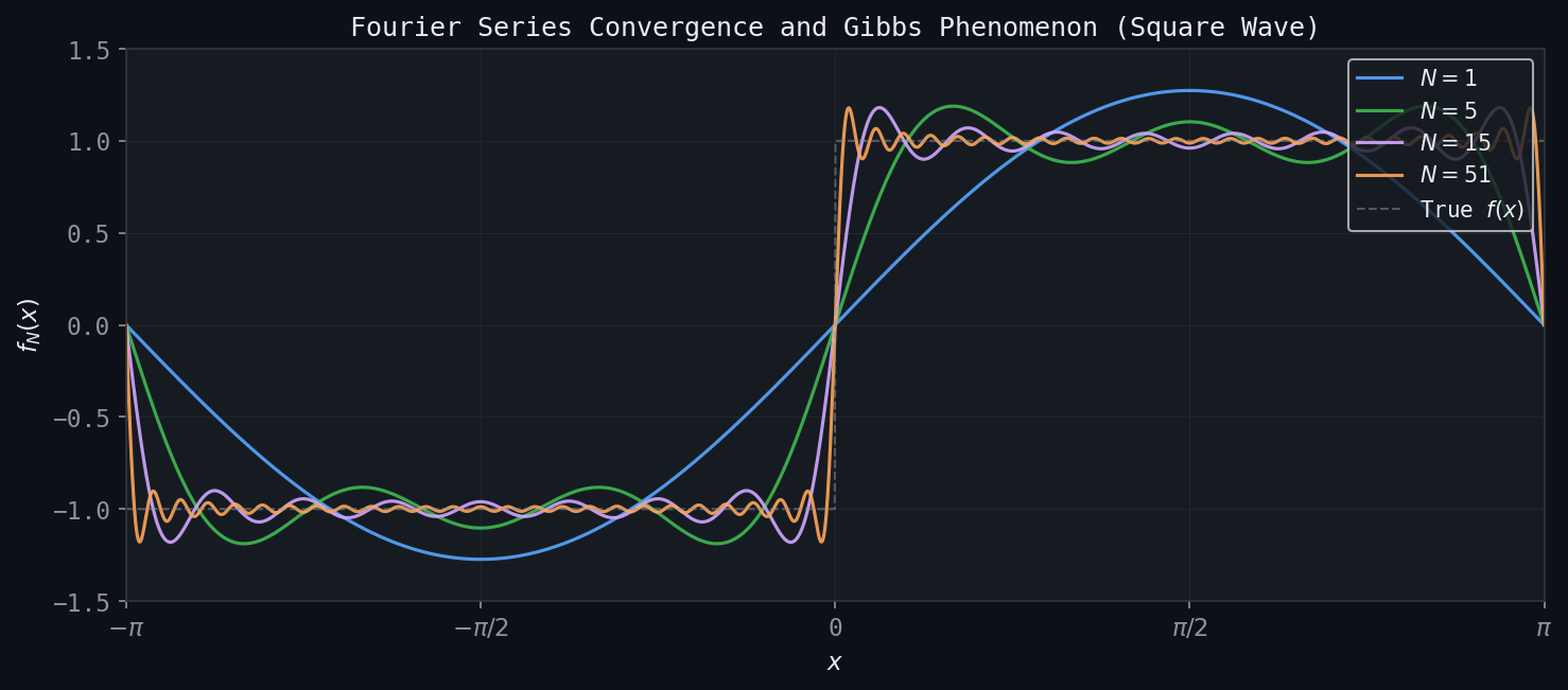Figure: Partial Fourier sums for the square wave at N=1, 5, 15, 51. Near the jump discontinuity, the ~9% Gibbs overshoot persists regardless of N.

When the Fourier series partial sum is used to approximate a function with a jump discontinuity, a characteristic overshoot appears near the discontinuity that does not diminish as the number of terms increases — it merely becomes more localized. This is the Gibbs phenomenon: the partial sum overshoots the true function value by approximately \(9\%\) of the jump height on each side of the discontinuity, regardless of how many terms are included.

\[ S_N(x) = \frac{4}{\pi}\sum_{k=0}^{N-1} \frac{\sin((2k+1)x)}{2k+1}. \]

Near \(x = 0\), the maximum overshoot approaches \(\frac{1}{\pi}\int_0^\pi \frac{\sin t}{t} dt - \frac{1}{2} \approx 0.0895\), which is roughly \(9\%\) of the total jump of 2.

The Gibbs phenomenon is not a failure of the Fourier series per se — the series does converge in \(L^2\) and even pointwise — but rather a consequence of the global nature of the trigonometric basis functions. This motivates the development of representations that are better adapted to local behavior, which is ultimately what wavelets provide.

5.5 Parseval’s Theorem for Fourier Series

\[ \frac{1}{2\pi}\int_{-\pi}^{\pi} |f(x)|^2 \, dx = \sum_{k=-\infty}^{\infty} |c_k|^2. \]

In signal processing language, this says that the total power of the signal equals the sum of powers at each frequency. It establishes an isometric isomorphism between \(L^2[-\pi,\pi]\) and the sequence space \(\ell^2(\mathbb{Z})\).

---

Chapter 6: The Discrete Fourier Transform

6.1 From Fourier Series to the DFT

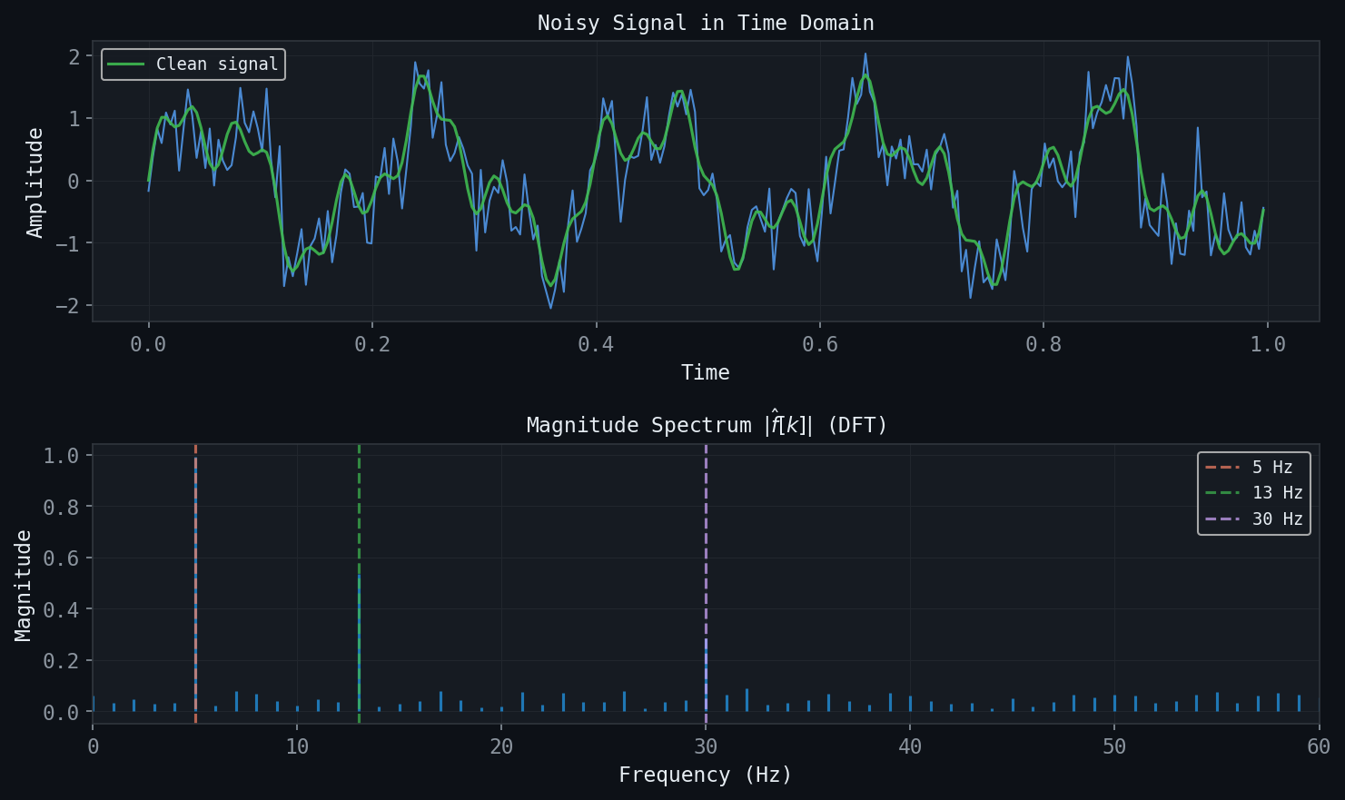Figure: A noisy signal (top) and its DFT magnitude spectrum (bottom). The three component frequencies at 5, 13, and 30 Hz are clearly identified despite noise.

In practice, signals are sampled at finitely many points, and one works with vectors in \(\mathbb{C}^N\) rather than functions in \(L^2\). The Discrete Fourier Transform (DFT) is the analogue of the Fourier series for such finite discrete signals.

\[ \hat{x}_k = \sum_{n=0}^{N-1} x_n \, \omega^{-kn}, \quad k = 0, 1, \ldots, N-1, \]

where \(\omega = e^{2\pi i/N}\) is the primitive \(N\)-th root of unity.

The key insight is that the vectors \(\mathbf{v}_k = \frac{1}{\sqrt{N}}(1, \omega^k, \omega^{2k}, \ldots, \omega^{(N-1)k})\) for \(k = 0, 1, \ldots, N-1\) form an orthonormal basis for \(\mathbb{C}^N\). In \(\mathbb{C}^N\) the inner product is \(\langle \mathbf{u}, \mathbf{v} \rangle = \sum_n u_n \overline{v_n}\), and one can verify \(\langle \mathbf{v}_j, \mathbf{v}_k \rangle = \delta_{jk}\).

6.2 Conventions and Versions

The DFT has several equivalent formulations that differ in sign conventions and normalization. This course uses three main versions:

Version 1 (analysis): \(\hat{x}_k = \sum_{n=0}^{N-1} x_n \, \omega^{-kn}\).

Version 2 (inverse): \(x_n = \frac{1}{N} \sum_{k=0}^{N-1} \hat{x}_k \, \omega^{kn}\).

Version 3 (symmetric/unitary): Both analysis and synthesis include a factor of \(1/\sqrt{N}\).

\[ \mathbf{F}_N = \frac{1}{\sqrt{N}} \left[\omega^{-jk}\right]_{j,k=0}^{N-1} \]

is a unitary matrix: \(\mathbf{F}_N^\dagger \mathbf{F}_N = \mathbf{I}\). This is the matrix expression of the orthonormality of the Fourier basis vectors.

6.3 Properties of the DFT

The DFT possesses a rich set of algebraic properties that make it useful for computation and analysis.

Linearity. The DFT is a linear map: \(\widehat{\alpha \mathbf{x} + \beta \mathbf{y}} = \alpha \hat{\mathbf{x}} + \beta \hat{\mathbf{y}}\).

Conjugate symmetry. If \(\mathbf{x}\) is real-valued, then \(\hat{x}_{N-k} = \overline{\hat{x}_k}\). This means the spectrum is symmetric: the information in the upper half of the frequency range is redundant.

Circular shift. If \(\mathbf{y}\) is obtained from \(\mathbf{x}\) by a circular shift of \(m\) positions — \(y_n = x_{n-m \mod N}\) — then \(\hat{y}_k = \omega^{-km} \hat{x}_k\). A time shift corresponds to multiplication by a phase factor in the frequency domain.

\[ (\mathbf{x} * \mathbf{y})_n = \sum_{m=0}^{N-1} x_m y_{n-m \mod N}. \]

Then \(\widehat{\mathbf{x} * \mathbf{y}} = \hat{\mathbf{x}} \cdot \hat{\mathbf{y}}\) (pointwise multiplication). This convolution theorem is the key to efficient filtering in the frequency domain.

Parseval’s identity for DFT. \(\sum_{n=0}^{N-1} |x_n|^2 = \frac{1}{N} \sum_{k=0}^{N-1} |\hat{x}_k|^2\) (Version 1 convention), or simply \(\|\mathbf{x}\|^2 = \|\hat{\mathbf{x}}\|^2\) in the unitary convention.

6.4 The Fast Fourier Transform

Direct computation of the DFT requires \(O(N^2)\) operations (multiplications and additions). The Fast Fourier Transform (FFT) is an algorithm that exploits the recursive structure of the DFT matrix when \(N\) is a power of 2, reducing the complexity to \(O(N \log N)\).

\[ \hat{x}_k = \hat{x}_k^{\text{even}} + \omega^{-k} \hat{x}_k^{\text{odd}}, \quad k = 0, 1, \ldots, \frac{N}{2}-1. \]

Applying this decomposition recursively yields \(O(N\log_2 N)\) operations. For \(N = 2^{20} \approx 10^6\), this represents a speedup by a factor of roughly \(N/\log_2 N \approx 50{,}000\) over the naive approach — a difference that makes real-time signal processing possible in practice.

---

Chapter 7: DFT Applications — Signal and Image Processing

7.1 Signal Compression and Thresholding

A powerful application of the DFT is signal compression via frequency-domain thresholding. Given a signal \(\mathbf{x} \in \mathbb{R}^N\), one computes its DFT coefficients \(\hat{\mathbf{x}}\), retains only those coefficients with largest magnitude (setting the rest to zero), and reconstructs with the inverse DFT. If the signal has a smooth or periodic structure, most of its energy will concentrate in a small number of frequency components, and the reconstruction from a small fraction of coefficients will be visually or acoustically indistinguishable from the original.

If one retains the \(M\) largest DFT coefficients (out of \(N\)), the compression ratio is \(N/M\). The reconstruction error depends on the decay rate of the coefficients: for a smooth signal whose coefficients decay rapidly, aggressive compression incurs little distortion.

Hard thresholding sets all coefficients below a threshold \(\tau\) to zero, producing a sparse representation. Soft thresholding additionally reduces the magnitude of large coefficients, trading some fidelity for improved noise robustness.

7.2 Signal Denoising

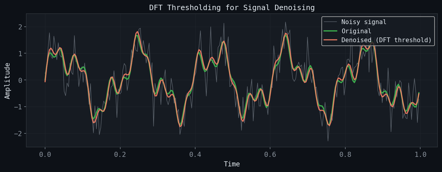Figure: DFT thresholding denoising. Setting Fourier coefficients below a threshold to zero recovers the clean signal.

In the denoising problem, one observes a signal \(\mathbf{y} = \mathbf{x} + \boldsymbol{\eta}\), where \(\mathbf{x}\) is the clean signal and \(\boldsymbol{\eta}\) represents additive noise. If the clean signal has energy concentrated at low frequencies and the noise is spread across all frequencies, then frequency-domain thresholding effectively separates signal from noise.

The procedure is: compute the DFT, zero out or attenuate the high-frequency components that correspond to noise, then reconstruct. The threshold \(\tau\) controls the trade-off between noise reduction and signal distortion.

7.3 The 2D DFT and Image Processing

\[ \hat{X}_{jk} = \sum_{m=0}^{M-1}\sum_{n=0}^{N-1} X_{mn} \, e^{-2\pi i(jm/M + kn/N)}. \]

This is computed efficiently as a sequence of 1D FFTs applied first to rows and then to columns.

Low-frequency components (near the center of the 2D spectrum in the shifted convention) correspond to slowly varying background intensities; high-frequency components carry edge and texture information. Image sharpening (high-frequency boosting) and blurring (low-frequency filtering) are straightforward in the Fourier domain.

7.4 The Discrete Cosine Transform and JPEG Compression

\[ \hat{x}_k = \sqrt{\frac{2}{N}} c_k \sum_{n=0}^{N-1} x_n \cos\!\left(\frac{\pi k (2n+1)}{2N}\right), \]

where \(c_0 = 1/\sqrt{2}\) and \(c_k = 1\) for \(k \geq 1\).

The JPEG compression standard exploits the DCT in a blockwise fashion. The image is divided into non-overlapping \(8 \times 8\) pixel blocks. Each block is transformed with the 2D DCT. The resulting 64 DCT coefficients per block are quantized (rounded to coarser values), and the quantized coefficients are encoded using Huffman coding. The human visual system is less sensitive to high-frequency coefficients than to low-frequency ones, so aggressive quantization of the high-frequency entries produces visually acceptable images with high compression ratios.

---

Chapter 8: The Continuous Fourier Transform

8.1 Definition and Basic Properties

\[ \hat{f}(\xi) = \int_{-\infty}^{\infty} f(x) e^{-2\pi i \xi x} \, dx, \]\[ f(x) = \int_{-\infty}^{\infty} \hat{f}(\xi) e^{2\pi i \xi x} \, d\xi. \]

The CFT shares many properties with the DFT:

• Linearity: \(\widehat{\alpha f + \beta g} = \alpha \hat{f} + \beta \hat{g}\).
• Shift: If \(g(x) = f(x - x_0)\), then \(\hat{g}(\xi) = e^{-2\pi i \xi x_0} \hat{f}(\xi)\).
• Modulation: If \(g(x) = e^{2\pi i \xi_0 x} f(x)\), then \(\hat{g}(\xi) = \hat{f}(\xi - \xi_0)\).
• Convolution theorem: \(\widehat{f * g}(\xi) = \hat{f}(\xi) \hat{g}(\xi)\), where \((f * g)(x) = \int f(y)g(x-y) \, dy\).
• Differentiation: \(\widehat{f'}(\xi) = 2\pi i \xi \hat{f}(\xi)\); the Fourier transform converts differentiation to multiplication.

8.2 The Gaussian and Its Transform

\[ g_\sigma(x) = e^{-\pi x^2/\sigma^2} \implies \hat{g}_\sigma(\xi) = \sigma \, e^{-\pi \sigma^2 \xi^2}. \]

A narrow Gaussian in time has a wide Fourier transform, and vice versa. This reciprocal relationship is a concrete manifestation of the uncertainty principle, treated in detail in Chapter 9.

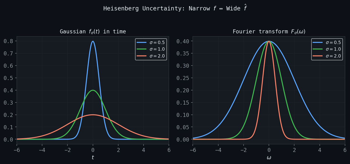Figure: The time-frequency trade-off for Gaussians. A narrow time-domain Gaussian (small \(\sigma\)) has a wide Fourier transform, and vice versa.

8.3 The Plancherel and Parseval Theorems

\[ \int_{-\infty}^{\infty} |f(x)|^2 \, dx = \int_{-\infty}^{\infty} |\hat{f}(\xi)|^2 \, d\xi, \]\[ \int_{-\infty}^{\infty} f(x)\overline{g(x)} \, dx = \int_{-\infty}^{\infty} \hat{f}(\xi)\overline{\hat{g}(\xi)} \, d\xi. \]

8.4 The Dirac Delta and Generalized Functions

The Dirac delta \(\delta(x)\) is not a function in the classical sense but rather a generalized function (distribution), defined by its action on test functions: \(\int \delta(x) \phi(x) dx = \phi(0)\). Its Fourier transform is the constant function: \(\hat{\delta}(\xi) = 1\). Conversely, the Fourier transform of the constant function \(f(x) = 1\) is \(\hat{f}(\xi) = \delta(\xi)\).

These relations are essential for understanding the Fourier transform of periodic functions (which are not in \(L^1\) or \(L^2\)) and for deriving the Sampling Theorem in Chapter 9.

8.5 The Heat Equation and Diffusion

\[ \frac{\partial u}{\partial t} = \frac{\partial^2 u}{\partial x^2}, \quad u(x, 0) = f(x). \]\[ u(x, t) = f * G_t(x), \quad G_t(x) = \frac{1}{\sqrt{4\pi t}} e^{-x^2/(4t)}, \]

where \(G_t\) is the Gaussian heat kernel. At small \(t\), \(G_t\) is narrowly concentrated and the solution is close to the initial data; as \(t\) increases, the Gaussian broadens, smoothing the solution.

High-frequency components are damped by the factor \(e^{-(2\pi\xi)^2 t}\), which decreases rapidly with frequency for any \(t > 0\). The heat equation is therefore a low-pass filter: it smooths the initial data by attenuating high frequencies.

Anisotropic diffusion, motivated by image processing, replaces the uniform diffusion coefficient with a spatially varying one that is small near edges (to preserve them) and large in smooth regions (to aggressively smooth noise). This nonlinear PDE-based approach preserves structural features while removing texture noise.

---

Chapter 9: Time-Frequency Analysis and the Uncertainty Principle

9.1 The Sampling Theorem

A central question in signal processing is: given a continuous bandlimited signal, how densely must it be sampled to permit perfect reconstruction?

A function \(f \in L^2(\mathbb{R})\) is bandlimited with bandwidth \(\Omega\) (in Hz) if its Fourier transform satisfies \(\hat{f}(\xi) = 0\) for \(|\xi| > \Omega\). The Whittaker-Shannon sampling theorem answers the reconstruction question precisely:

The derivation proceeds by noting that since \(\hat{f}\) has support in \([-\Omega, \Omega]\), one can expand \(\hat{f}\) as a Fourier series on this interval, and the Fourier coefficients of this series are exactly the sampled values \(f(n/(2\Omega))\). The reconstruction formula then follows from the inverse Fourier transform.

Sampling below the Nyquist rate causes aliasing: high-frequency components appear as spurious low-frequency artifacts in the reconstructed signal. In audio processing, aliasing sounds like ringing or distortion; in image processing, it manifests as Moiré patterns or “jaggies” on diagonal lines.

9.2 Interpolation

Before digital-to-analog conversion, discrete sample values must be interpolated. Three common schemes arise naturally:

Piecewise-constant (zero-order hold): \(f(t) \approx f(n\Delta t)\) for \(t \in [n\Delta t, (n+1)\Delta t)\). This is computationally simple but introduces a staircase artifact and a sinc-shaped frequency response that attenuates high frequencies.

Piecewise-linear (first-order hold): Linear interpolation between adjacent samples. Smoother than piecewise-constant, with frequency response proportional to \(\operatorname{sinc}^2\), which decays faster and introduces less distortion.

Sinc interpolation (ideal): Using the cardinal series with sinc basis functions. This is the theoretically exact reconstruction for bandlimited signals, but the sinc function has infinite support, making it impractical for real-time applications. Windowed sinc functions (multiplied by a smooth taper) provide a practical approximation.

9.3 The Uncertainty Principle

\[ \Delta_t^2 = \frac{\int t^2 |f(t)|^2 \, dt}{\int |f(t)|^2 \, dt}, \qquad \Delta_\xi^2 = \frac{\int \xi^2 |\hat{f}(\xi)|^2 \, d\xi}{\int |\hat{f}(\xi)|^2 \, d\xi}, \]

measuring the second moment of the energy distribution in time and frequency, respectively.

The proof uses integration by parts and the Cauchy-Schwarz inequality. The result says that any attempt to localize a signal in time (small \(\Delta_t\)) must spread its frequency content (large \(\Delta_\xi\)), and vice versa. The Gaussian achieves the optimal trade-off.

The finite support theorem is a complementary result: a nonzero function \(f\) and its Fourier transform \(\hat{f}\) cannot both have finite support. If \(f\) is compactly supported, then \(\hat{f}\) must extend to all of \(\mathbb{R}\), and vice versa.

9.4 The Short-Time Fourier Transform

The global nature of the Fourier transform — each coefficient \(\hat{f}(\xi)\) depends on the entire signal \(f(t)\) — makes it ill-suited to signals whose frequency content changes over time. The Short-Time Fourier Transform (STFT) or Gabor transform addresses this by first multiplying \(f\) by a localized window function before Fourier transforming.

\[ (\mathcal{G}f)(b, \xi) = \int_{-\infty}^{\infty} f(t) \, g(t - b) \, e^{-2\pi i \xi t} \, dt, \]

where \(b\) is the time localization parameter and \(\xi\) is frequency. For each fixed \(b\), one is computing the ordinary Fourier transform of \(f\) restricted to a neighborhood of time \(b\). The result is a two-dimensional representation on the time-frequency plane.

The uncertainty principle limits the resolution of the STFT: the window \(g\) determines fixed time and frequency resolutions, \(\Delta_t(g)\) and \(\Delta_\xi(g)\), that cannot simultaneously be made arbitrarily small. A narrow window \(g\) gives good time resolution but poor frequency resolution; a wide window gives good frequency resolution but poor time resolution. The STFT is therefore limited to a fixed rectangular “tile” in the time-frequency plane for all frequencies.

A chirped signal \(f(t) = e^{i\phi(t)}\) has instantaneous frequency \(\phi'(t)/(2\pi)\) that varies over time. The STFT reveals the time-varying frequency content as a ridge in the time-frequency plane, tracing the chirp trajectory. However, the fixed window size of the STFT is suboptimal for signals with very different rates of variation at different scales — motivating the wavelet transform.

---

Chapter 10: Wavelets and the Haar System

10.1 Motivation: Multi-Scale Analysis

The limitation of the STFT — fixed resolution in the time-frequency plane — motivates a transform that automatically adapts its resolution to the scale of the features being analyzed. The wavelet transform uses dilated and translated versions of a single “mother wavelet” function, achieving fine time resolution at high frequencies and fine frequency resolution at low frequencies.

Intuitively, high-frequency features (sharp edges, transient events) are brief and require fine time sampling; they are also well-isolated in time so one does not need fine frequency resolution there. Low-frequency features (trends, slowly varying structure) are spread over long times and require fine frequency resolution; precise time localization is less critical. The wavelet transform respects this natural trade-off.

10.2 Piecewise-Constant Approximations and the Haar System

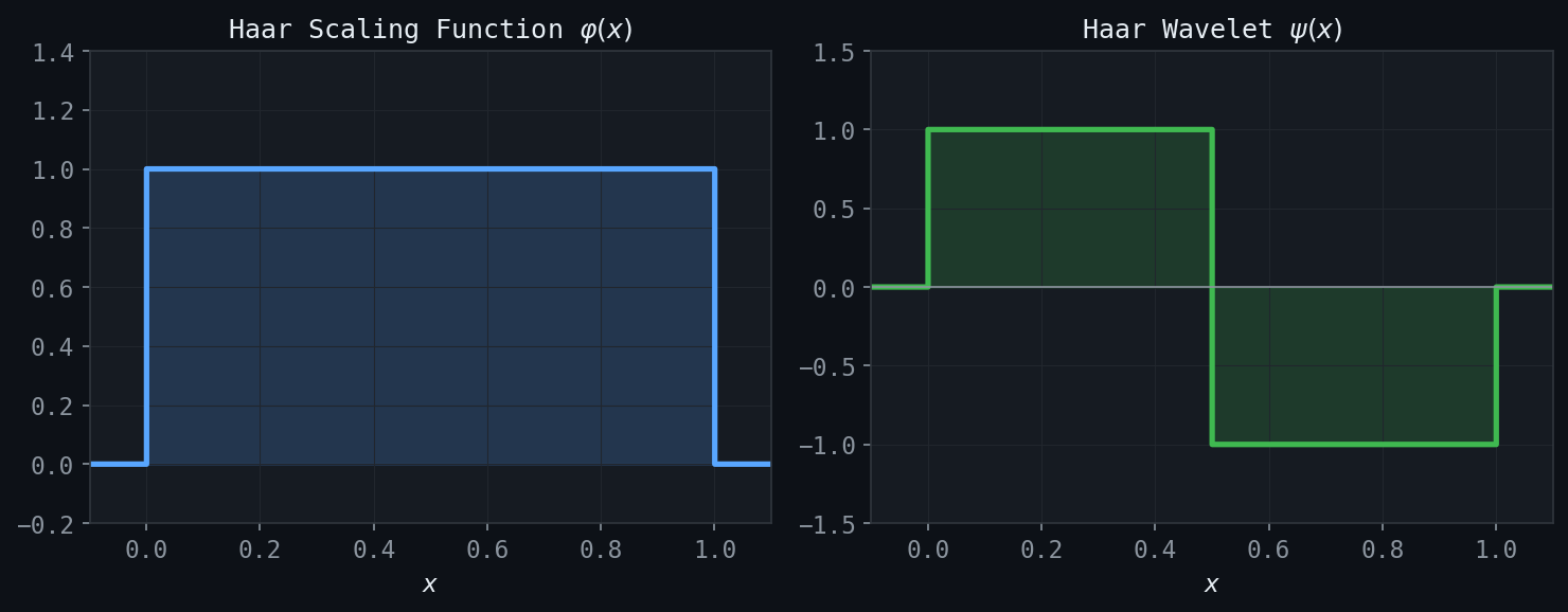Figure: The Haar scaling function \(\varphi(x) = \mathbf{1}_{[0,1)}(x)\) (left) and the Haar wavelet \(\psi(x)\) (right).

The simplest wavelet system, and the key pedagogical example, is the Haar system, which arises naturally from piecewise-constant approximations to signals.

Consider approximating a function \(f \in L^2[0,1]\) by piecewise-constant functions at various resolutions. At resolution \(j\), one divides \([0,1]\) into \(2^j\) equal subintervals of width \(2^{-j}\), and approximates \(f\) by its average value on each subinterval.

\[ \varphi(t) = \chi_{[0,1)}(t) = \begin{cases} 1 & 0 \leq t < 1 \\ 0 & \text{otherwise.}\end{cases} \]

Its translates and dilates \(\varphi_{jk}(t) = 2^{j/2} \varphi(2^j t - k)\) for \(k = 0, 1, \ldots, 2^j - 1\) form an orthonormal basis for the space \(V_j\) of piecewise-constant functions at resolution \(j\).

\[ f_j(t) = \sum_k a_{jk} \varphi_{jk}(t), \quad a_{jk} = \langle f, \varphi_{jk} \rangle = 2^{j/2} \int_{k \cdot 2^{-j}}^{(k+1) \cdot 2^{-j}} f(t) \, dt. \]

As \(j \to \infty\), \(f_j \to f\) in \(L^2\). As \(j \to -\infty\), \(f_j \to 0\) in \(L^2\).

10.3 The Haar Wavelet

The spaces \(V_j\) are nested: \(V_0 \subset V_1 \subset V_2 \subset \cdots\), because any piecewise-constant function at resolution \(j\) is also piecewise-constant at the finer resolution \(j+1\). The detail added when going from resolution \(j\) to resolution \(j+1\) lives in the orthogonal complement \(W_j = V_{j+1} \ominus V_j\), defined by the condition \(V_{j+1} = V_j \oplus W_j\) (orthogonal direct sum).

\[ \psi(t) = \begin{cases} +1 & 0 \leq t < 1/2 \\ -1 & 1/2 \leq t < 1 \\ 0 & \text{otherwise.}\end{cases} \]

The family \(\psi_{jk}(t) = 2^{j/2}\psi(2^j t - k)\) is an orthonormal basis for \(W_j\). One can verify directly: \(\langle \psi_{j k}, \psi_{j' k'} \rangle = \delta_{jj'}\delta_{kk'}\) for all \(j, j', k, k'\).

\[ L^2(\mathbb{R}) = \bigoplus_{j=-\infty}^{\infty} W_j = \cdots \oplus W_{-1} \oplus W_0 \oplus W_1 \oplus \cdots \]

Equivalently, \(V_j = V_0 \oplus W_0 \oplus W_1 \oplus \cdots \oplus W_{j-1}\) for any \(j \geq 1\). The entire space \(L^2(\mathbb{R})\) is decomposed into mutually orthogonal detail spaces, each carrying information at a distinct scale.

10.4 Haar Wavelets on a Finite Interval

For practical computation on signals of length \(N = 2^J\) (indexed \(0, 1, \ldots, N-1\)), one works with the finite discrete Haar system. Given a signal vector \(\mathbf{a}_J = (a_{J,0}, a_{J,1}, \ldots, a_{J,N-1})\), the Haar wavelet analysis (decomposition) algorithm computes detail coefficients at each level:

\[ a_{j-1,k} = \frac{1}{\sqrt{2}}\left(a_{j,2k} + a_{j,2k+1}\right), \quad b_{j-1,k} = \frac{1}{\sqrt{2}}\left(a_{j,2k} - a_{j,2k+1}\right). \]

Here \(a_{j-1,k}\) is the average (approximation) coefficient and \(b_{j-1,k}\) is the difference (detail or wavelet) coefficient. At each step, the number of coefficients halves; after \(J\) steps, one has a single coarsest average coefficient \(a_{0,0}\) plus detail coefficients \(\{b_{j,k}\}\) at all scales \(j = 0, 1, \ldots, J-1\).

These detail and approximation coefficients organize naturally into a wavelet coefficient tree, with the coarsest approximation at the root and finer detail coefficients at each successive level. This hierarchical structure is the hallmark of multi-scale analysis.

10.5 The Haar Synthesis (Reconstruction) Algorithm

The inverse transform reconstructs the original signal from the wavelet coefficients:

\[ a_{j,2k} = \frac{1}{\sqrt{2}}\left(a_{j-1,k} + b_{j-1,k}\right), \quad a_{j,2k+1} = \frac{1}{\sqrt{2}}\left(a_{j-1,k} - b_{j-1,k}\right). \]

Reconstruction is exact: the original signal is recovered without error, since the Haar transform is orthonormal.

For compression, one applies the analysis transform, zeroes out small detail coefficients (those below a threshold), and reconstructs. Because signals often have most of their energy in coarse-scale approximation coefficients, the Haar transform achieves good compression ratios for piecewise-constant or piecewise-smooth signals.

---

Chapter 11: Multiresolution Analysis

11.1 The General MRA Framework

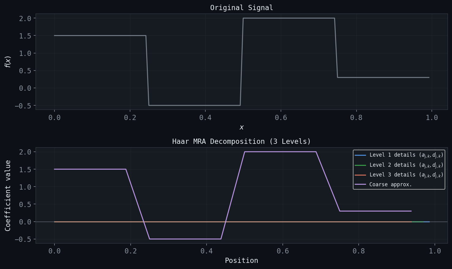Figure: Three-level Haar MRA decomposition. The original signal (top) is progressively separated into coarse approximations and detail coefficients at each scale.

The Haar system is a special case of a broad mathematical structure called Multiresolution Analysis (MRA), introduced by Mallat and Meyer in the 1980s. An MRA provides the systematic framework for constructing general wavelet families with prescribed properties.

The Haar system satisfies all five axioms with \(\varphi = \chi_{[0,1)}\).

11.2 The Scaling Equation (Two-Scale Relation)

\[ \varphi(t) = \sqrt{2} \sum_{k} h_k \, \varphi(2t - k). \]

The real numbers \(\{h_k\}\) are the scaling coefficients. For the Haar scaling function, \(h_0 = h_1 = 1/\sqrt{2}\) and \(h_k = 0\) for \(k \notin \{0,1\}\).

\[ \hat{\varphi}(\xi) = H(\xi/2) \hat{\varphi}(\xi/2), \quad H(\xi) = \frac{1}{\sqrt{2}} \sum_k h_k e^{-2\pi i k \xi}, \]

where \(H(\xi)\) is the (normalized) discrete Fourier transform of the filter \(\{h_k\}\). Iterating: \(\hat{\varphi}(\xi) = \prod_{j=1}^{\infty} H(\xi/2^j)\).

11.3 The Wavelet Function and the QMF Conditions

\[ \psi(t) = \sqrt{2} \sum_k g_k \, \varphi(2t - k), \quad g_k = (-1)^k h_{1-k}. \]

The sign-alternating, time-reversed relationship \(g_k = (-1)^k h_{1-k}\) is the wavelet analogue of the quadrature mirror filter relationship in signal processing.

For the family \(\{\psi_{jk}\} = \{2^{j/2}\psi(2^j t - k)\}\) to be an orthonormal basis for the detail spaces, the filter \(\{h_k\}\) must satisfy the Quadrature Mirror Filter (QMF) conditions:

1. \(\displaystyle\sum_k h_k^2 = 1\) (normalization),
2. \(\displaystyle\sum_k h_k h_{k-2p} = \delta_{p,0}\) for all \(p \in \mathbb{Z}\) (orthogonality of even translates),
3. \(\displaystyle\sum_k h_k = \sqrt{2}\) (ensures \(\int \varphi(t) \, dt = 1\)).

Equivalently, conditions 1 and 2 state that \(|H(\xi)|^2 + |H(\xi + 1/2)|^2 = 1\), i.e., the filter \(H\) and its half-shift together constitute a perfect reconstruction filter bank.

11.4 The General Analysis and Synthesis Algorithms

For a general MRA, the analysis and synthesis algorithms are identical in structure to the Haar case, but use the general filter coefficients \(\{h_k\}\) and \(\{g_k\}\) instead of the simple averages and differences.

\[ a_{j-1,m} = \sum_k h_{k-2m} \, a_{j,k}, \quad b_{j-1,m} = \sum_k g_{k-2m} \, a_{j,k}. \]

In signal processing terms, this is filtering \(\{a_{j,k}\}\) with the low-pass filter \(\{h_k\}\) and high-pass filter \(\{g_k\}\), followed by downsampling (keeping every other sample).

\[ a_{j,k} = \sum_m h_{k-2m} \, a_{j-1,m} + \sum_m g_{k-2m} \, b_{j-1,m}. \]

This is upsampling each set of coefficients (inserting zeros between samples), then filtering and summing.

The filter bank interpretation makes the connection to digital signal processing explicit: the analysis step is a two-channel filter bank with low-pass and high-pass branches, each followed by decimation; the synthesis step is the dual expansion and combination step.

11.5 The Shannon MRA

\[ \varphi(t) = \operatorname{sinc}(t) = \frac{\sin(\pi t)}{\pi t}. \]

The corresponding space \(V_0\) consists of all bandlimited functions with bandwidth at most \(1/2\): functions whose Fourier transforms are supported in \([-1/2, 1/2]\). More generally, \(V_j\) consists of functions bandlimited to \([-2^j/2, 2^j/2]\).

The Shannon MRA satisfies all five MRA axioms. However, the sinc scaling function has infinite support in time — it is not localized and its integer translates decay only algebraically. The corresponding wavelet is also non-compactly supported. The Shannon MRA is therefore of theoretical interest (it connects MRA theory directly to the sampling theorem) but is impractical for computation.

---

Chapter 12: Wavelet Families and Daubechies Wavelets

12.1 The Wavelet Function and Its Zero-Mean Property

\[ \int_{-\infty}^{\infty} \psi(t) \, dt = 0. \]

This follows from the QMF conditions: \(\sum_k g_k = \sum_k (-1)^k h_{1-k} = 0\) because the sum of \(h_k\) with alternating signs vanishes (it equals \(H(1/2)\), and the QMF condition requires \(|H(1/2)| = 0\)). In the Fourier domain, this reads \(\hat{\psi}(0) = 0\): the wavelet has no DC component. Wavelets are inherently oscillatory — the word “wavelet” (French: \textit{ondelette}) means “little wave.”

12.2 Vanishing Moments

\[ \int_{-\infty}^{\infty} t^k \psi(t) \, dt = 0, \quad k = 0, 1, 2, \ldots, M-1. \]

In other words, \(\psi\) is orthogonal to all polynomials of degree less than \(M\).

The zero-mean condition is the \(k=0\) case. The number of vanishing moments measures how “smooth” the wavelet’s interaction with the signal is: if a signal is locally well-approximated by a polynomial of degree less than \(M\), its wavelet coefficients at fine scales will be small.

\[ |b_{j,k}| \leq C \cdot 2^{-j(M + 1/2)} \|f^{(M)}\|_{L^2}, \]

for any function \(f\) whose \(M\)-th derivative is in \(L^2\). Wavelet coefficients decay at rate \(2^{-jM}\) in scale — faster when the wavelet has more vanishing moments and when the signal is smoother.

12.3 The Daubechies Wavelets

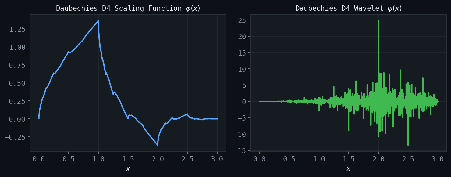Figure: Daubechies D4 scaling function (left) and wavelet (right), computed via the cascade algorithm. D4 has two vanishing moments and compact support on \([0,3]\).

Ingrid Daubechies constructed families of wavelets that achieve maximum vanishing moments for a given filter length, while maintaining the MRA structure, real coefficients, and orthonormality. The Daubechies-\(N\) wavelet (with \(N\) even) uses \(N\) nonzero scaling coefficients \(h_0, h_1, \ldots, h_{N-1}\) and has \(N/2\) vanishing moments.

Daubechies-2 (D2) = Haar. The simplest case uses \(h_0 = h_1 = 1/\sqrt{2}\), giving \(M=1\) vanishing moment. The scaling function is the unit step and the wavelet is the Haar function.

\[ h_0 = \frac{1+\sqrt{3}}{4\sqrt{2}}, \quad h_1 = \frac{3+\sqrt{3}}{4\sqrt{2}}, \quad h_2 = \frac{3-\sqrt{3}}{4\sqrt{2}}, \quad h_3 = \frac{1-\sqrt{3}}{4\sqrt{2}}. \]

The D4 wavelet has \(M=2\) vanishing moments and compact support \([0,3]\). It provides significantly better approximation than the Haar wavelet for smooth signals.

Daubechies-6 (D6), D8, D10, \ldots Increasing \(N\) gives more vanishing moments and smoother scaling functions and wavelets, at the cost of longer support \([0, N-1]\) and more expensive computation. The Daubechies-\(N\) wavelet has support \([0, N-1]\) and \(N/2\) vanishing moments.

The Daubechies coefficients are determined by the QMF conditions together with a maximum flatness condition: the filter \(H(\xi)\) should have as many zeros as possible at \(\xi = 1/2\) (the highest frequency). Specifically, \(H(\xi) = \left(\frac{1+e^{-2\pi i\xi}}{2}\right)^{N/2} L(\xi)\) where \(L\) is chosen to satisfy the remaining QMF conditions and to have real, minimum-phase coefficients.

12.4 Compact Support and Its Consequences

For any MRA scaling function, the number of nonzero scaling coefficients is finite if and only if \(\varphi\) has compact support. The Daubechies construction produces compactly supported wavelets: the scaling function \(\varphi\) and mother wavelet \(\psi\) both have support of length \(N-1\).

Compact support has major practical consequences:

• The analysis and synthesis algorithms require only finitely many operations per coefficient, making them efficient.
• Boundary effects are limited to a region of size proportional to the support length.
• Storage of wavelet coefficients is efficient.

In contrast, the Shannon wavelet (based on the sinc function) has infinite support, making it impractical despite its theoretical elegance.

12.5 Hölder Regularity

The Daubechies scaling functions and wavelets are continuous for \(N \geq 4\), but they are generally not differentiable. Their Hölder regularity (the exponent \(\alpha\) such that \(|\varphi(t) - \varphi(s)| \leq C|t-s|^\alpha\)) increases with \(N\). The Haar scaling function is discontinuous (Hölder exponent 0); D4 has positive Hölder exponent roughly \(0.55\); D10 has Hölder exponent approximately \(1.08\) and is thus continuously differentiable.

For signal processing, the smoothness of the wavelet affects the perceptual quality of compressed or denoised signals: smooth wavelets produce cleaner reconstructions, while the Haar wavelet’s discontinuities can introduce blocking artifacts.

\[ \|f - P_{V_j} f\|_{L^2} \leq C \cdot 2^{-jM} \|f^{(M)}\|_{L^2} \]

for any \(f \in H^M(\mathbb{R})\) (the Sobolev space of \(M\)-times weakly differentiable functions in \(L^2\)). This theorem quantifies how rapidly the approximation error decreases as the resolution level \(j\) is refined: more vanishing moments produce faster convergence for smooth functions.

12.6 Fourier Analysis of MRA

\[ \sum_{k \in \mathbb{Z}} |\hat{\varphi}(\xi + k)|^2 = 1 \quad \text{for a.e. } \xi. \]\[ \sum_k |\hat{\varphi}(\xi + k)|^2 = |H(\xi/2)|^2 \sum_k |\hat{\varphi}(\xi/2 + k)|^2 + |H(\xi/2 + 1/2)|^2 \sum_k |\hat{\varphi}(\xi/2 + 1/2 + k)|^2 = 1, \]

which leads to the QMF condition \(|H(\xi)|^2 + |H(\xi + 1/2)|^2 = 1\).

The wavelet satisfies \(\hat{\psi}(\xi) = G(\xi/2)\hat{\varphi}(\xi/2)\) with \(G(\xi) = e^{-2\pi i\xi} \overline{H(\xi + 1/2)}\), ensuring that \(\psi\) has zero mean (\(\hat{\psi}(0) = 0\)) and that the family \(\{\psi_{jk}\}\) is an orthonormal basis for \(L^2(\mathbb{R})\).

12.7 Wavelet-Based Denoising and Compression

The superior performance of Daubechies wavelets over Haar in practical applications arises from the combination of compact support (computational efficiency), vanishing moments (sparse representation of smooth signals), and regularity (perceptual quality). A comparison of Haar and D4 applied to a smooth signal illustrates:

• Haar: many nonzero detail coefficients even in smooth regions, because the Haar wavelet (with only 1 vanishing moment) responds to any linear variation within its support.
• D4: few nonzero detail coefficients in smooth regions, because the D4 wavelet (with 2 vanishing moments) is orthogonal to both constants and linear functions; only near discontinuities or sharp features does it produce large coefficients.

For wavelet denoising, one applies the following procedure: (1) compute the multi-level wavelet transform; (2) threshold the detail coefficients (hard or soft thresholding); (3) reconstruct. The Donoho-Johnstone theory shows that, for the right threshold and wavelet choice, this procedure achieves the optimal minimax rate of denoising for functions in broad regularity classes.

For image compression (the wavelet-based JPEG 2000 standard uses Daubechies-9/7 biorthogonal wavelets), the same principle applies: natural images have sparse representations in the wavelet domain because they are piecewise smooth. Large coefficients occur only near edges; the smooth regions contribute few large wavelet coefficients. Aggressive thresholding of small coefficients, followed by quantization and lossless coding, achieves high compression ratios with perceptually high quality.

---

Summary

This course has traced a path from the abstract foundations of functional analysis to the most modern tools of applied harmonic analysis. The key conceptual thread is best approximation in Hilbert spaces: the Fourier series, the DFT, the wavelet expansion, and the MRA framework are all instantiations of the projection theorem — the best approximation of \(f\) in a subspace is its orthogonal projection, and all the coefficients are inner products.

The progression from Fourier series to wavelets is driven by the need for increasingly adaptive representations:

1. Fourier series and DFT: optimal for periodic, globally regular signals; global in space.
2. STFT/Gabor transform: local in time but with fixed resolution; good for stationary or nearly-stationary signals.
3. Wavelet transform (Haar and MRA): multi-scale, automatically adaptive; efficient for piecewise-smooth signals.
4. Daubechies wavelets: compact support + vanishing moments + regularity = optimal for practical compression and denoising.

The mathematical framework — metric completeness, Hilbert space geometry, the projection theorem, Parseval’s identity, and the QMF conditions — underlies all of these representations and unifies what might otherwise appear as a collection of ad hoc algorithms.