Chapter 1: Introduction to Discrete Models

What Are Discrete Models?

Mathematics offers two broad languages for describing how quantities change over time: the continuous and the discrete. In the continuous setting, governed by differential equations, time flows without interruption, and the instantaneous rate of change of a quantity is related to its current value. In the discrete setting, quantities are measured or updated only at separated instants — at each tick of a clock, each generation of a population, each day of an investment period. The equations that describe this kind of evolution are called difference equations, and they form the central object of study in this course.

A difference equation expresses the value of a quantity at one moment in terms of its value (or values) at previous moments. If we label the sequence of values as \( x_0, x_1, x_2, \ldots \), a typical first-order rule might say that \( x_{n+1} \) is determined entirely by \( x_n \). Such a rule, together with a starting value \( x_0 \), completely determines the entire future evolution of the sequence. This makes discrete models conceptually clean and computationally transparent: to simulate the system, one simply applies the rule repeatedly.

Why Study Discrete Models?

Discrete models arise naturally whenever the underlying phenomenon is itself discrete. Populations that reproduce in seasonal bursts — annual plants, insects with fixed breeding seasons, fish stocks measured at yearly intervals — evolve in discrete time. Financial instruments such as loans, mortgages, and compound-interest accounts accrue in discrete steps. Digital signal processing, numerical algorithms, and computer simulations all operate in discrete time by necessity.

Beyond these practical motivations, discrete dynamical systems exhibit a remarkable richness of behaviour. Even the simplest nonlinear difference equations can produce trajectories that oscillate, cycle, or wander in a manner so complex as to appear random. This phenomenon — chaos — was one of the great discoveries of twentieth-century mathematics, and it first appeared clearly in discrete systems. The logistic map, a one-parameter family of quadratic functions of an interval to itself, serves as the canonical example and will occupy much of the latter half of this course.

From Differential Equations to Difference Equations: The Euler Method

One important source of difference equations is numerical analysis. When a differential equation cannot be solved in closed form, one common approach is Euler’s method: divide time into small steps of size \( h \), and approximate the derivative \( \dot{x} = f(x, t) \) by a forward difference \( (x_{n+1} - x_n)/h \). Rearranging,

\[ x_{n+1} = x_n + h \, f(x_n, t_n). \]

This is a first-order difference equation in \( x_n \). Euler’s method is the simplest numerical integrator; more accurate methods (Runge-Kutta, Adams-Bashforth) produce more involved difference equations, but all share the same discrete-time structure. The analysis of these methods — their stability, accuracy, and long-time behaviour — is itself a branch of discrete dynamical systems theory.

Basic Terminology

A difference equation of order \( k \) is a relation of the form

\[ F(n, x_n, x_{n+1}, \ldots, x_{n+k}) = 0, \]

where \( F \) is some specified function and \( k \geq 1 \). The equation is linear if \( F \) is linear in all the \( x \) variables, and nonlinear otherwise. It has constant coefficients if the coefficients multiplying the \( x \) terms do not depend on \( n \). A difference equation is autonomous if \( n \) does not appear explicitly, so the rule governing evolution is the same at every time step. The order of a difference equation is analogous to the order of a differential equation: a first-order equation involves only two consecutive values \( x_n \) and \( x_{n+1} \), while a second-order equation involves three consecutive values \( x_{n-1}, x_n, x_{n+1} \).

To solve a difference equation of order \( k \), one must specify \( k \) initial conditions — typically \( x_0, x_1, \ldots, x_{k-1} \) — after which the equation determines all subsequent values uniquely. A solution is a sequence \( \{x_n\}_{n=0}^\infty \) satisfying the equation for all \( n \geq 0 \).

Financial Mathematics as a Motivating Application

Perhaps the most familiar context for difference equations is compound interest. Suppose an account earns interest at a rate \( r \) per period (say, per year). If \( x_n \) denotes the balance after \( n \) periods, then

\[ x_{n+1} = (1 + r) x_n. \]

This is a first-order linear difference equation with constant coefficients. Starting from an initial deposit \( x_0 = P \), the solution is immediately seen to be

\[ x_n = P (1 + r)^n, \]

the familiar compound-interest formula. If, in addition, a fixed payment \( b \) is deposited (or withdrawn) at each period, the equation becomes

\[ x_{n+1} = (1 + r) x_n + b, \]

which is a nonhomogeneous first-order linear equation. These simple models already capture the essential features of mortgages, annuities, and savings plans, and they motivate the general theory of first-order linear difference equations developed in the next chapter.

---

Chapter 2: First-Order Linear Difference Equations

The General First-Order Linear Equation

A first-order linear difference equation with constant coefficients takes the form

\[ x_{n+1} = a x_n + b, \]

where \( a \) and \( b \) are given constants. When \( b = 0 \), the equation is called homogeneous; when \( b \neq 0 \), it is nonhomogeneous. This single equation, seemingly modest, encapsulates an enormous range of applications: compound interest, population growth with immigration, drug dosage models, and radioactive decay with a constant source, to name a few.

Solving by Iteration

The most direct approach to solving \( x_{n+1} = a x_n + b \) is simply to apply the equation repeatedly. Starting from \( x_0 \),

\[ x_1 = a x_0 + b, \quad x_2 = a x_1 + b = a^2 x_0 + ab + b, \quad x_3 = a^3 x_0 + a^2 b + ab + b, \]

and in general

\[ x_n = a^n x_0 + b(a^{n-1} + a^{n-2} + \cdots + 1). \]

When \( a \neq 1 \), the geometric sum evaluates to \( (a^n - 1)/(a - 1) \), giving

\[ x_n = a^n x_0 + b \cdot \frac{a^n - 1}{a - 1}. \]

When \( a = 1 \), the equation reduces to \( x_{n+1} = x_n + b \), and the solution is simply \( x_n = x_0 + nb \), an arithmetic progression.

Fixed Points and Stability

A fixed point (or equilibrium) of the difference equation is a constant solution \( x_n = \bar{x} \) for all \( n \). Substituting into \( x_{n+1} = a x_n + b \), we require \( \bar{x} = a \bar{x} + b \), which gives

\[ \bar{x} = \frac{b}{1 - a}, \quad \text{provided } a \neq 1. \]

The long-term behaviour of solutions depends critically on the parameter \( a \). Writing \( y_n = x_n - \bar{x} \) for the deviation from equilibrium, the equation for \( y_n \) is

\[ y_{n+1} = a y_n, \]

whose solution is \( y_n = a^n y_0 \). Thus \( x_n \to \bar{x} \) as \( n \to \infty \) if and only if \( |a| < 1 \). In this case the fixed point is called stable (or attracting). If \( |a| > 1 \), deviations grow without bound and the fixed point is unstable (or repelling). The boundary case \( |a| = 1 \) requires separate analysis.

A Biological Application: Drug Dosage

Consider a patient who takes a drug dose of \( D \) units at regular intervals of time \( T \). Between doses, the body eliminates a fraction \( (1 - a) \) of the drug present, where \( 0 < a < 1 \) is the retention factor. If \( x_n \) denotes the drug level just after the \( n \)-th dose, then

\[ x_{n+1} = a x_n + D. \]

Here \( a \) and \( D \) play the roles of the parameters in the general first-order equation. The fixed point is \( \bar{x} = D/(1-a) \), which represents the steady-state drug level. Since \( |a| < 1 \), the fixed point is stable, and the drug level converges to \( \bar{x} \) regardless of the initial dose. The physician must choose \( D \) and the dosing interval (which affects \( a \)) so that the steady-state level lies within the therapeutic window — high enough to be effective but low enough to avoid toxicity.

A Financial Application: Mortgages

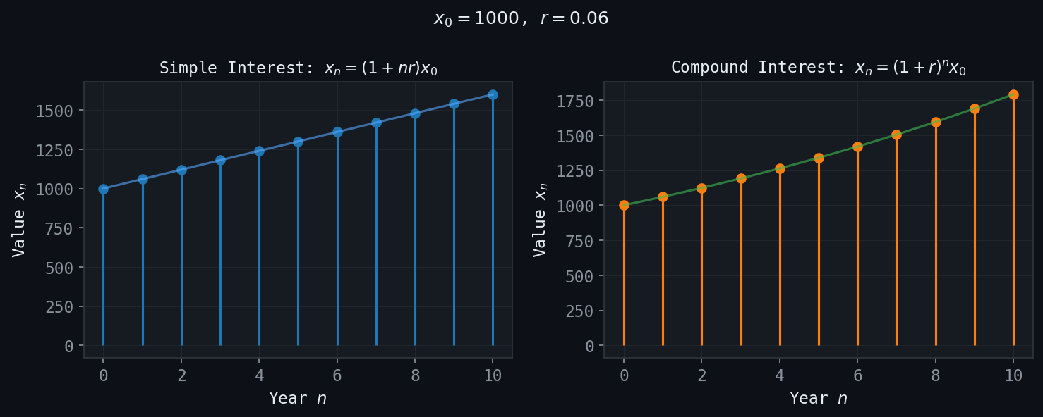Figure: Linear (simple) vs. exponential (compound) growth of an investment over 10 years.

A mortgage is a loan of amount \( P \) to be repaid in equal monthly payments of \( m \) dollars. If the monthly interest rate is \( r \) (annual rate divided by 12), and \( x_n \) denotes the outstanding balance after \( n \) months, then

\[ x_{n+1} = (1 + r) x_n - m. \]

This is a first-order linear equation with \( a = 1 + r > 1 \) and \( b = -m \). The fixed point is \( \bar{x} = m/r \). Since \( a > 1 \), the fixed point is unstable: if the balance starts below \( m/r \) (because payments are large enough), the balance decreases toward zero and the loan is repaid; if it starts above \( m/r \) (payments too small), the balance grows without bound. The standard calculation for the monthly payment that retires the loan in exactly \( N \) months sets \( x_N = 0 \) and solves for \( m \).

---

Chapter 3: Second-Order Linear Difference Equations

The General Second-Order Equation

A second-order linear difference equation with constant coefficients has the form

\[ x_{n+1} + p x_n + q x_{n-1} = 0 \]

for the homogeneous case, or

\[ x_{n+1} + p x_n + q x_{n-1} = f(n) \]

for the nonhomogeneous case, where \( p \), \( q \), and the forcing function \( f(n) \) are given. Two initial conditions \( x_0 \) and \( x_1 \) uniquely determine the entire solution sequence.

The Characteristic Equation

The key to solving second-order linear equations is the observation that solutions of exponential form \( x_n = m^n \) may exist. Substituting into the homogeneous equation:

\[ m^{n+1} + p m^n + q m^{n-1} = 0. \]

Dividing by \( m^{n-1} \) (for \( m \neq 0 \)) yields the characteristic equation

\[ m^2 + pm + q = 0. \]

The nature of the roots of this quadratic determines the form of the general solution.

Case 1: Two Distinct Real Roots

If the discriminant \( p^2 - 4q > 0 \), the characteristic equation has two distinct real roots \( m_1 \) and \( m_2 \). The general solution is

\[ x_n = c_1 m_1^n + c_2 m_2^n, \]

where \( c_1 \) and \( c_2 \) are arbitrary constants determined by the initial conditions.

Case 2: Repeated Real Root

If \( p^2 - 4q = 0 \), there is a single real root \( m = -p/2 \) of multiplicity two. In this case the two independent solutions are \( m^n \) and \( n m^n \), giving the general solution

\[ x_n = (c_1 + c_2 n) m^n. \]

The appearance of the factor \( n \) is analogous to the repeated-root case in ordinary differential equations, where the second independent solution acquires a factor of \( t \).

Case 3: Complex Conjugate Roots

If \( p^2 - 4q < 0 \), the roots are complex conjugates \( m_{1,2} = \alpha \pm \beta i \). It is most convenient to write them in polar form: \( m_{1,2} = r e^{\pm i\theta} \), where the modulus is \( r = \sqrt{\alpha^2 + \beta^2} = \sqrt{q} \) and the argument is \( \theta = \arctan(\beta/\alpha) \). The general real-valued solution is

\[ x_n = r^n (c_1 \cos(n\theta) + c_2 \sin(n\theta)). \]

This solution exhibits oscillatory behaviour with amplitude growing as \( r^n \) (if \( r > 1 \)), decaying (if \( r < 1 \)), or constant (if \( r = 1 \)). The frequency of oscillation is determined by \( \theta \).

The Fibonacci Sequence

The Fibonacci sequence is defined by the recurrence

\[ F_{n+1} = F_n + F_{n-1}, \quad F_0 = 0, \quad F_1 = 1. \]

This is a homogeneous second-order linear equation with \( p = -1 \) and \( q = -1 \). The characteristic equation is \( m^2 - m - 1 = 0 \), with roots

\[ m_{1,2} = \frac{1 \pm \sqrt{5}}{2}. \]

The larger root \( \phi = (1 + \sqrt{5})/2 \approx 1.618 \) is the celebrated golden ratio. The general solution is

\[ F_n = c_1 \phi^n + c_2 \psi^n, \quad \text{where } \psi = \frac{1 - \sqrt{5}}{2} \approx -0.618. \]

Applying the initial conditions \( F_0 = 0 \) and \( F_1 = 1 \) gives \( c_1 = 1/\sqrt{5} \) and \( c_2 = -1/\sqrt{5} \), yielding Binet’s formula:

\[ F_n = \frac{1}{\sqrt{5}} \left[ \left(\frac{1 + \sqrt{5}}{2}\right)^n - \left(\frac{1 - \sqrt{5}}{2}\right)^n \right]. \]

Remarkably, this formula involving irrational numbers always produces an integer. Since \( |\psi| < 1 \), the term \( \psi^n / \sqrt{5} \) tends to zero, so \( F_n \) is the nearest integer to \( \phi^n / \sqrt{5} \). The ratio of successive Fibonacci numbers \( F_{n+1}/F_n \to \phi \) as \( n \to \infty \).

An Annual Plant Propagation Model

Consider an annual plant species in which each individual lives for one year, produces seeds, and then dies. Let \( x_n \) denote the population size in year \( n \). Seeds germinate in the following year, and some fraction also lie dormant for an additional year. If a fraction \( a \) of seeds germinate immediately and a fraction \( b \) of this year’s seeds lie dormant and germinate next year, the population satisfies

\[ x_{n+1} = a x_n + b x_{n-1}. \]

This is precisely a second-order linear equation. The characteristic roots determine whether the population grows, decays, or oscillates. Such models are foundational in theoretical ecology.

---

Chapter 4: Nonhomogeneous Difference Equations

Structure of the General Solution

The general solution of a nonhomogeneous linear difference equation

\[ x_{n+1} + p x_n + q x_{n-1} = f(n) \]

has the form

\[ x_n = x_n^{(h)} + x_n^{(p)}, \]

where \( x_n^{(h)} \) is the general solution of the corresponding homogeneous equation (with \( f = 0 \)), and \( x_n^{(p)} \) is any particular solution of the nonhomogeneous equation. This principle of superposition holds because the equation is linear.

Method of Undetermined Coefficients

The method of undetermined coefficients provides particular solutions when the forcing function \( f(n) \) belongs to a class of functions that is “closed” under the operations of the difference operator. The method proceeds by guessing the form of the particular solution based on the form of \( f(n) \), and then determining the unknown coefficients by substitution.

The standard cases are organised as follows.

Resonance

The crucial subtlety arises when the natural frequency of the forcing function coincides with a characteristic root of the homogeneous equation. In this situation — called resonance — the standard guess for the particular solution is itself a solution of the homogeneous equation and therefore gives \( 0 = 0 \) upon substitution. The fix is to multiply the trial solution by \( n \) (or \( n^k \) if the root has multiplicity \( k \)). This is entirely analogous to the resonance phenomenon in second-order linear ODEs.

---

Chapter 5: Linear Systems of Difference Equations

Vector Formulation

Many models involve several interacting quantities that all evolve simultaneously in discrete time. A linear system of difference equations takes the form

\[ \mathbf{x}_{n+1} = A \mathbf{x}_n, \]

where \( \mathbf{x}_n \in \mathbb{R}^k \) is a vector of state variables and \( A \) is a \( k \times k \) matrix of constant coefficients. This formulation also subsumes higher-order scalar equations: a \( k \)-th order scalar equation can always be converted to a first-order system in \( k \) dimensions by introducing the state vector \( \mathbf{x}_n = (x_n, x_{n-1}, \ldots, x_{n-k+1})^T \).

Solution via Eigenvalues and Eigenvectors

The solution of \( \mathbf{x}_{n+1} = A\mathbf{x}_n \) is, formally, \( \mathbf{x}_n = A^n \mathbf{x}_0 \). To compute \( A^n \) efficiently, one diagonalizes \( A \). Suppose \( A \) has \( k \) linearly independent eigenvectors \( \mathbf{v}_1, \ldots, \mathbf{v}_k \) with corresponding eigenvalues \( \lambda_1, \ldots, \lambda_k \). Then any initial condition can be written as

\[ \mathbf{x}_0 = c_1 \mathbf{v}_1 + c_2 \mathbf{v}_2 + \cdots + c_k \mathbf{v}_k, \]

and the solution is

\[ \mathbf{x}_n = c_1 \lambda_1^n \mathbf{v}_1 + c_2 \lambda_2^n \mathbf{v}_2 + \cdots + c_k \lambda_k^n \mathbf{v}_k. \]

Each eigenvector defines an invariant line through the origin: if the initial condition lies exactly along \( \mathbf{v}_i \), the trajectory stays on that line and is simply scaled by \( \lambda_i \) at each step.

Stable and Unstable Eigenspaces

The long-term behaviour of the system is dominated by the eigenvalue of largest modulus. If \( |\lambda_1| > |\lambda_j| \) for all \( j \neq 1 \), then for a generic initial condition the solution grows like \( |\lambda_1|^n \mathbf{v}_1 \) as \( n \to \infty \).

One can partition the state space into:

• The stable eigenspace \( E^s \): the span of eigenvectors corresponding to eigenvalues with \( |\lambda| < 1 \). Trajectories starting in \( E^s \) converge to the origin.
• The unstable eigenspace \( E^u \): the span of eigenvectors corresponding to eigenvalues with \( |\lambda| > 1 \). Trajectories starting in \( E^u \) diverge from the origin.

The origin \( \mathbf{x} = \mathbf{0} \) is a stable fixed point if all eigenvalues satisfy \( |\lambda_i| < 1 \), and unstable if any eigenvalue satisfies \( |\lambda_i| > 1 \).

A Red Blood Cell Production Model

A classical application is the model of red blood cell production. Let \( R_n \) denote the number of red blood cells in circulation at time step \( n \), and let \( M_n \) denote the concentration of a control hormone (such as erythropoietin) that stimulates production. A simplified model assumes:

\[ R_{n+1} = (1 - \gamma) R_n + \beta M_n, \]\[ M_{n+1} = \alpha R_n - \delta M_n, \]

where \( \gamma \) is the daily destruction rate of red blood cells, \( \beta \) is the sensitivity of cell production to the hormone, \( \alpha \) is the feedback gain from cell count to hormone production, and \( \delta \) is the hormone decay rate. Written in matrix form, \( \mathbf{x}_{n+1} = A \mathbf{x}_n \) with

\[ A = \begin{pmatrix} 1 - \gamma & \beta \\ \alpha & -\delta \end{pmatrix}. \]

The stability of this system (whether red blood cell counts converge to a normal level, oscillate, or diverge) is determined by the eigenvalues of \( A \). Oscillating solutions correspond to complex eigenvalues with \( |\lambda| \approx 1 \) and can model pathological conditions such as periodic anemia.

---

Chapter 6: Nonlinear Dynamics and Fixed Points

Beyond Linearity

Linear difference equations are tractable because the superposition principle holds: sums of solutions are again solutions, and the geometry of the solution space is simple. Real-world systems, however, are rarely linear. Population growth is constrained by resources, chemical reactions saturate, and competition between species produces genuinely nonlinear dynamics. The study of nonlinear difference equations requires new tools: cobweb diagrams, Lyapunov functions, and the local linearization technique.

Cobweb Diagrams

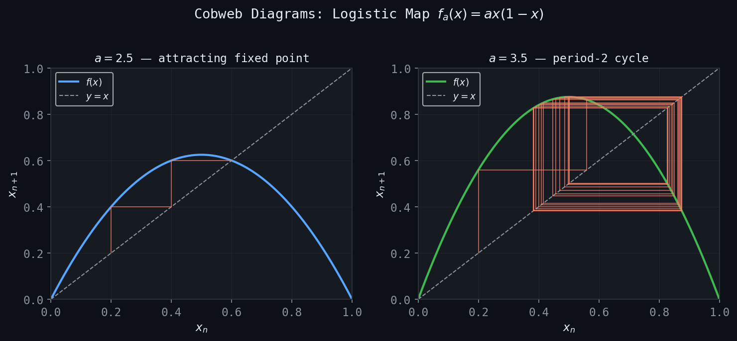Figure: Cobweb diagrams for \(f_a(x) = ax(1-x)\). Left: attracting fixed point at \(a=2.5\). Right: period-2 orbit at \(a=3.5\).

For a first-order autonomous equation \( x_{n+1} = f(x_n) \), one of the most powerful visualization tools is the cobweb diagram (also called a Lamerey diagram). One plots the curve \( y = f(x) \) and the diagonal \( y = x \) in the same plane. Starting from \( x_0 \), one draws a vertical line to the curve — reaching \( (x_0, f(x_0)) = (x_0, x_1) \) — then a horizontal line to the diagonal — reaching \( (x_1, x_1) \) — then again a vertical line to the curve, and so on. The resulting “cobweb” pattern visually traces the entire orbit of \( x_0 \).

Fixed points appear as intersections of \( y = f(x) \) with the diagonal \( y = x \). Near a stable fixed point, cobweb trajectories spiral inward (for complex-like dynamics) or converge monotonically (when \( f'(\bar{x}) > 0 \)). Near an unstable fixed point, they diverge.

Fixed Points and Local Stability

A fixed point of the map \( f : \mathbb{R} \to \mathbb{R} \) is a value \( \bar{x} \) satisfying \( f(\bar{x}) = \bar{x} \). The local stability of \( \bar{x} \) is determined by the derivative of \( f \) at that point. Linearizing the equation near \( \bar{x} \) by setting \( x_n = \bar{x} + \epsilon_n \) for small \( \epsilon_n \):

\[ \bar{x} + \epsilon_{n+1} = f(\bar{x} + \epsilon_n) \approx f(\bar{x}) + f'(\bar{x}) \epsilon_n = \bar{x} + f'(\bar{x}) \epsilon_n, \]

so \( \epsilon_{n+1} \approx f'(\bar{x}) \epsilon_n \). This is a linear first-order equation with multiplier \( a = f'(\bar{x}) \).

Periodic Points

A point \( x_0 \) is a periodic point of period \( p \) if \( f^p(x_0) = x_0 \) but \( f^k(x_0) \neq x_0 \) for \( 0 < k < p \), where \( f^p \) denotes the \( p \)-fold composition of \( f \) with itself. Period-2 points are fixed points of \( f^2 \) that are not fixed points of \( f \); they satisfy \( f(f(x)) = x \) but \( f(x) \neq x \).

The stability of a period-\( p \) orbit is determined by the chain rule for the derivative of the composed map: if \( \{x_0, x_1, \ldots, x_{p-1}\} \) is a period-\( p \) orbit, then

\[ (f^p)'(x_0) = f'(x_0) f'(x_1) \cdots f'(x_{p-1}). \]

The orbit is stable if \( |(f^p)'(x_0)| < 1 \) and unstable if \( |(f^p)'(x_0)| > 1 \).

---

Chapter 7: The Logistic Map and Period Doubling

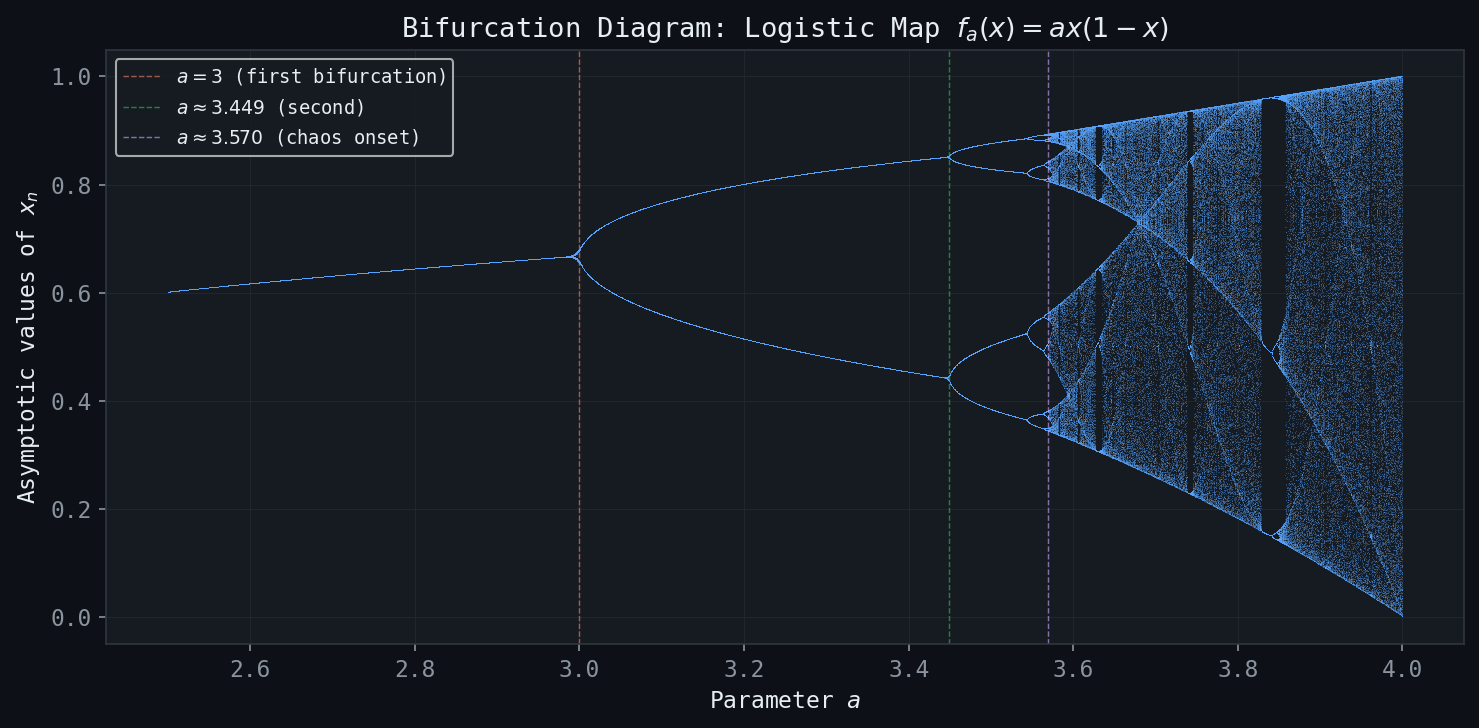Figure: The bifurcation diagram of \(f_a(x) = ax(1-x)\), showing period-doubling cascades leading to chaos.

The Logistic Map

The logistic map is the function

\[ f_a(x) = ax(1 - x), \quad x \in [0, 1], \]

parameterized by \( a \in (0, 4] \). When \( a \leq 4 \), the map sends \( [0,1] \) into itself. The logistic map is the canonical model of population growth with a carrying capacity: the factor \( x \) represents the current population (normalized to the interval \( [0,1] \)), and the factor \( (1-x) \) represents the restraining effect of limited resources. The parameter \( a \) is the intrinsic growth rate.

Fixed Points

The fixed points of \( f_a \) satisfy \( f_a(x) = x \), i.e., \( ax(1-x) = x \). This gives \( x(a(1-x) - 1) = 0 \), so the fixed points are

\[ \bar{x}_1 = 0, \qquad \bar{x}_2 = \frac{a-1}{a}. \]

Note that \( \bar{x}_2 \in (0,1) \) only when \( a > 1 \).

The derivatives are \( f_a'(x) = a(1 - 2x) \), giving

\[ f_a'(\bar{x}_1) = a, \qquad f_a'(\bar{x}_2) = 2 - a. \]

Thus:

• \( \bar{x}_1 = 0 \) is stable when \( |a| < 1 \), i.e., \( 0 < a < 1 \).
• \( \bar{x}_2 = (a-1)/a \) is stable when \( |2 - a| < 1 \), i.e., \( 1 < a < 3 \).
• At \( a = 3 \), the derivative at \( \bar{x}_2 \) equals \( -1 \), and a bifurcation occurs.

Period-Doubling Bifurcations

At \( a = 3 \), the fixed point \( \bar{x}_2 \) loses stability. Just past this value, a period-2 orbit is born: two points \( x^*, x^{**} \) with \( f_a(x^*) = x^{**} \) and \( f_a(x^{**}) = x^* \). This is the first in an infinite cascade of period-doubling bifurcations.

As \( a \) increases through a sequence of critical values \( a_1 < a_2 < a_3 < \cdots \), each stable period-\( 2^k \) orbit loses stability and gives birth to a stable period-\( 2^{k+1} \) orbit:

• For \( 1 < a < 3 \): stable fixed point.
• For \( 3 < a < 1 + \sqrt{6} \approx 3.449 \): stable period-2 orbit.
• For \( 1 + \sqrt{6} < a < a_3 \approx 3.544 \): stable period-4 orbit.
• Continuing, the critical values \( a_k \) accumulate to \( a_\infty \approx 3.5699 \).

The Feigenbaum Constant

The critical values \( a_k \) at which period-doublings occur converge to \( a_\infty \) with a geometric rate. The ratio of successive gaps converges to the Feigenbaum constant:

\[ \delta = \lim_{k \to \infty} \frac{a_k - a_{k-1}}{a_{k+1} - a_k} \approx 4.6692. \]

This constant is universal: the same value \( \delta \approx 4.6692 \) appears in the period-doubling cascade of any smooth unimodal map with a quadratic maximum. Feigenbaum’s discovery in the late 1970s was one of the first rigorous results on universality in the transition to chaos.

The Bifurcation Diagram

A bifurcation diagram provides a comprehensive summary of the dynamics. For each value of the parameter \( a \), one iterates the map \( f_a \) many times from a generic starting point (discarding the transient), then plots the remaining iterates as a function of \( a \). The result is a tree-like structure: a single branch for \( 1 < a < 3 \) (the stable fixed point), which splits into two branches at \( a = 3 \), splits again at \( a \approx 3.449 \), and so on. Beyond \( a_\infty \), the diagram shows a dense, apparently random scatter — the chaotic regime — interrupted by windows of periodic behaviour (most prominently a period-3 window near \( a \approx 3.83 \)).

The period-3 window is notable because, by Sharkovskii’s theorem, the existence of a period-3 orbit implies the existence of orbits of every period. The slogan “period three implies chaos” (Li and Yorke, 1975) was one of the first precise mathematical statements connecting periodic orbits to complex dynamics.

---

Chapter 8: Chaos and the Logistic Map

The Map \( f_4 \) and Its Iterates

At \( a = 4 \), the logistic map \( f_4(x) = 4x(1-x) \) is said to be chaotic in a precise mathematical sense. Understanding this requires first examining the graphs of iterated maps \( f_4^n(x) = f_4 \circ f_4 \circ \cdots \circ f_4 \) (\( n \) times).

The graph of \( f_4(x) \) is a single arch that rises from 0 to 1 and back to 0 on the unit interval. The graph of \( f_4^2(x) \) has two arches, that of \( f_4^3(x) \) has four, and in general \( f_4^n(x) \) has \( 2^{n-1} \) complete arches. This doubling property has a remarkable consequence: \( f_4^n \) intersects the diagonal \( y = x \) at exactly \( 2^n \) points, meaning \( f_4^n \) has exactly \( 2^n \) fixed points. These \( 2^n \) fixed points are precisely the periodic points of \( f_4 \) of period dividing \( n \).

Three Ingredients for Chaos

Modern mathematical analysis identifies three key properties that together constitute chaos in the sense of Devaney.

Dense Periodic Points

A subset \( S \) of a metric space \( X \) is dense in \( X \) if every open ball in \( X \) contains at least one point of \( S \). Equivalently, every point in \( X \) can be approximated to arbitrary precision by points in \( S \). The rationals are dense in the reals; the irrationals are also dense in the reals.

For \( f_4 \), the periodic points are dense in \( [0,1] \): near any point \( x \in [0,1] \), however close one looks, there is a periodic point of some period. This is a consequence of the doubling property: the \( 2^n \) fixed points of \( f_4^n \) are spread across the \( 2^{n-1} \) arches, and as \( n \to \infty \), they become arbitrarily dense.

Sensitive Dependence on Initial Conditions

Sensitive dependence on initial conditions (SDIC), also known as the butterfly effect, means that arbitrarily close initial conditions can lead to trajectories that diverge dramatically. Formally:

A sufficient condition for SDIC follows from the mean value theorem: if \( |f'(x)| \geq K > 1 \) for all \( x \) in an interval, then

\[ |f^n(x) - f^n(y)| \geq K^n |x - y|, \]

so nearby points separate exponentially fast. While \( f_4 \) is not uniformly expanding (its derivative vanishes at \( x = 1/2 \)), the geometry of its iterates still produces sensitive dependence over any neighbourhood.

Topological Transitivity

A map is topologically transitive if for any two non-empty open sets \( U \) and \( V \), there exists \( n > 0 \) such that \( f^n(U) \cap V \neq \emptyset \). Intuitively, this means the map “mixes” the space: orbits starting in any region will eventually visit any other region. Transitivity rules out the possibility that the dynamics splits into two or more independent subsystems.

The Tent Map and Baker Map

Two other maps are important for building intuition about chaos.

The tent map is defined by

\[ T(x) = \begin{cases} 2x, & 0 \leq x \leq 1/2 \\ 2(1-x), & 1/2 < x \leq 1. \end{cases} \]

It maps \( [0,1] \) into itself, has slope \( \pm 2 \) everywhere (away from \( x = 1/2 \)), and is conjugate to \( f_4 \) via the homeomorphism \( h(x) = \sin^2(\pi x/2) \). Because the tent map is piecewise linear with constant slope modulus 2, it is easier to analyze directly.

The Baker map (or doubling map) is

\[ B(x) = 2x \pmod{1}, \quad x \in [0,1). \]

This map is essentially multiplication by 2 modulo 1: it takes the binary expansion \( x = 0.b_1 b_2 b_3 \cdots \) (base 2) and shifts it left, producing \( B(x) = 0.b_2 b_3 b_4 \cdots \). The Baker map is chaotic, and it provides the cleanest entry point into symbolic dynamics.

---

Chapter 9: Symbolic Dynamics

The Space of Binary Sequences

Symbolic dynamics is a powerful technique that encodes the complex dynamics of a map by translating the trajectory of each initial condition into a sequence of symbols. The central object is the space of binary sequences

\[ \Sigma_2 = \{ (b_0, b_1, b_2, \ldots) : b_i \in \{0, 1\} \text{ for all } i \geq 0 \}. \]

This is an uncountable set; it can be put in bijection with \( [0,1] \) via binary expansions, though this correspondence has subtleties at dyadic rationals.

A natural metric on \( \Sigma_2 \) is

\[ d(\mathbf{b}, \mathbf{c}) = \sum_{i=0}^\infty \frac{|b_i - c_i|}{2^{i+1}}, \]

which makes \( \Sigma_2 \) a compact metric space. Two sequences are close in this metric if and only if they agree on a long initial block.

The Bernoulli Left-Shift

The Bernoulli left-shift \( S : \Sigma_2 \to \Sigma_2 \) is defined by

\[ S(b_0, b_1, b_2, \ldots) = (b_1, b_2, b_3, \ldots). \]

The shift simply discards the first symbol and advances all remaining symbols by one position. The shift map is continuous with respect to the metric on \( \Sigma_2 \) and is the archetypal model for symbolic dynamics.

Constructing a Dense Orbit

The existence of a dense orbit under \( S \) is constructive. One writes down the sequence that concatenates all finite binary strings in some order — for instance, listing them in order of increasing length: 0, 1, 00, 01, 10, 11, 000, 001, 010, \ldots — and concatenates them into one infinite sequence

\[ \mathbf{b}^* = (0 \mid 1 \mid 00 \mid 01 \mid 10 \mid 11 \mid 000 \mid 001 \mid \cdots). \]

For any open ball \( B_\varepsilon(\mathbf{c}) \) in \( \Sigma_2 \), there exists a finite initial segment that determines membership in the ball. Since every finite binary string appears somewhere in \( \mathbf{b}^* \), a shift of \( \mathbf{b}^* \) will eventually agree with \( \mathbf{c} \) on any finite number of initial symbols, placing it inside \( B_\varepsilon(\mathbf{c}) \).

The Baker Map and Symbolic Dynamics

The Baker map \( B(x) = 2x \pmod 1 \) is conjugate to the shift map \( S \) on \( \Sigma_2 \) via the encoding: each \( x \in [0,1) \) is identified with its binary expansion \( x = 0.b_0 b_1 b_2 \cdots \), and then

\[ B(x) = 0.b_1 b_2 b_3 \cdots \]

corresponds precisely to \( S(b_0, b_1, b_2, \ldots) = (b_1, b_2, b_3, \ldots) \). This identification shows that the dynamics of \( B \) is topologically conjugate to the dynamics of \( S \): the maps are the “same” in a dynamical sense, merely described in different coordinates. Since \( S \) is chaotic, so is \( B \).

Itinerary Sequences for the Tent Map and Logistic Map

The same symbolic coding works for the tent map \( T \) and the logistic map \( f_4 \). For the tent map, partition \( [0,1] \) into \( I_0 = [0, 1/2) \) and \( I_1 = [1/2, 1] \). The itinerary of \( x \) under \( T \) is the sequence \( \mathbf{b}(x) = (b_0, b_1, b_2, \ldots) \) where

\[ b_n = \begin{cases} 0 & \text{if } T^n(x) \in I_0, \\ 1 & \text{if } T^n(x) \in I_1. \end{cases} \]

One can show that the itinerary map \( x \mapsto \mathbf{b}(x) \) is a semiconjugacy between \( T \) and \( S \): \( \mathbf{b}(T(x)) = S(\mathbf{b}(x)) \). The same construction applies to \( f_4 \), confirming that all three maps — Baker, Tent, and Logistic at \( a = 4 \) — have isomorphic symbolic dynamics and are therefore all chaotic by the same argument.

Invariant Measures

A brief, non-examinable note on the statistical behavior of chaotic trajectories: even though individual trajectories are sensitive to initial conditions and difficult to predict, the long-run frequency with which a typical orbit visits different regions of the interval is well-defined and described by an invariant measure \( \mu \). For the tent map, the invariant measure is uniform (Lebesgue measure): almost every orbit spends equal time in equal-length subintervals. For \( f_4 \), the invariant measure has density

\[ \rho(x) = \frac{1}{\pi \sqrt{x(1-x)}}, \quad x \in (0,1), \]

the arcsine distribution. This density is large near \( x = 0 \) and \( x = 1 \) and small near \( x = 1/2 \), reflecting the fact that orbits of \( f_4 \) spend more time near the endpoints. These measures are connected to the ergodic theory of chaotic systems and provide a bridge between the deterministic chaos of individual trajectories and the probabilistic language of statistics.

---

Chapter 10: The Logistic Map for \( a > 4 \) and Cantor Sets

What Happens When \( a > 4 \)?

When \( a > 4 \), the logistic map \( f_a(x) = ax(1-x) \) no longer maps \( [0,1] \) into itself. Points near the centre of the interval are mapped outside \( [0,1] \), and once outside, the iterates diverge to \( -\infty \). The dynamics thus splits: some initial conditions escape to infinity, while others remain bounded forever. The set of bounded orbits forms a fractal invariant set.

More precisely, there exists an open interval \( J_1 \subset (0,1) \) that is mapped above 1 by \( f_a \). Define

\[ J_1 = \{ x \in [0,1] : f_a(x) > 1 \}. \]

Points in \( J_1 \) escape to \( -\infty \) in the next step. The preimage of \( J_1 \) consists of two intervals \( J_2 = J_{21} \cup J_{22} \), whose points map into \( J_1 \) in one step and then escape. Continuing, define \( J_{n+1} \) as the preimage of \( J_n \) under \( f_a \). The complement of all these escaping sets defines the invariant Cantor-like set

\[ C = [0,1] \setminus \bigcup_{n=0}^\infty J_n = \bigcap_{n=0}^\infty C_n, \]

where \( C_n = [0,1] \setminus (J_1 \cup J_2 \cup \cdots \cup J_n) \). The sets \( C_n \) are nested closed sets, and their intersection is the Cantor-like attractor for the restricted dynamics.

The Modified Tent Map and the Ternary Cantor Set

A cleaner construction arises from the modified tent map \( T_3 \), which stretches the middle third of \( [0,1] \) above 1:

\[ T_3(x) = \begin{cases} 3x, & 0 \leq x \leq 1/3 \\ 3(1-x)/2 + 1, & 1/3 < x < 2/3 \\ 3(1-x), & 2/3 \leq x \leq 1. \end{cases} \]

The interval \( J_1 = (1/3, 2/3) \) maps above 1. Its preimage \( J_2 \) consists of two intervals, each of length \( 1/9 \), located at the middle thirds of \( [0,1/3] \) and \( [2/3,1] \). Continuing, one removes middle thirds at every stage, generating the classical ternary Cantor set.

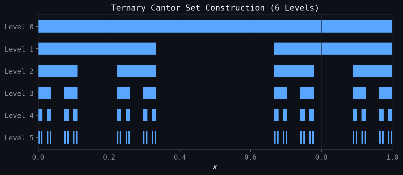Figure: Six levels of the ternary Cantor set construction. Each stage removes the open middle third of each remaining interval.

Properties of the Cantor Set

The Cantor set has several remarkable and at first counterintuitive properties.

Bounded and closed. Since each \( C_n \) is a closed bounded subset of \( \mathbb{R} \), and \( C \) is an intersection of closed sets, \( C \) itself is closed and bounded.

Zero total length. The total length removed in constructing \( C \) is

\[ \frac{1}{3} + \frac{2}{9} + \frac{4}{27} + \cdots = \frac{1/3}{1 - 2/3} = 1. \]

Every bit of length is removed, yet \( C \) is nonempty (it contains the endpoints of all removed intervals, among others).

Totally disconnected. Between any two points of \( C \), there is a removed interval. Formally, \( C \) contains no interval of positive length; every connected component of \( C \) is a single point.

Perfect. Every point of \( C \) is a limit point of \( C \): the set has no isolated points. Combined with total disconnectedness, this is a hallmark of fractal structure.

Uncountable. Despite having zero length, \( C \) is uncountable. One way to see this: each point \( x \in C \) has a ternary (base-3) expansion using only the digits 0 and 2 (no 1’s). The set of all such expansions bijects with the set of all binary sequences (replace 2 by 1), which is uncountable.

Newton-Raphson Method as a Dynamical System

The Newton-Raphson method for finding roots of a function \( f(x) \) generates the sequence

\[ x_{n+1} = N(x_n) = x_n - \frac{f(x_n)}{f'(x_n)}. \]

This defines a discrete dynamical system with the iteration function \( N(x) \). The zeros \( x^* \) of \( f \) are precisely the fixed points of \( N \): \( N(x^*) = x^* - 0 = x^* \). The derivative of \( N \) at a simple zero is

\[ N'(x^*) = 1 - \frac{(f'(x^*))^2 - f(x^*) f''(x^*)}{(f'(x^*))^2} = 0, \]

showing that every simple zero of \( f \) is a super-attracting fixed point of \( N \) (derivative exactly zero). This is why Newton’s method converges quadratically: the error at each step satisfies \( |x_{n+1} - x^*| \approx C |x_n - x^*|^2 \).

Newton’s Method in the Complex Plane and Julia Sets

When \( f \) is a polynomial with complex roots, Newton’s method becomes a map of the complex plane to itself. For \( f(z) = z^2 - 1 \), there are two roots \( z = \pm 1 \), and the plane divides into two basins of attraction — the set of initial conditions that converge to \( +1 \) and the set that converge to \( -1 \). The boundary between these basins (the Julia set of Newton’s method for this \( f \)) is a fractal curve.

For \( f(z) = z^3 - 1 \) with three cube roots of unity, the basins of attraction form an intricate fractal pattern. No matter how close one looks at the boundary between two basins, one always finds a trichromatic boundary: the three colors meet at every boundary point. This is a consequence of the Julia-Fatou theory, which provides the mathematical framework for classifying the dynamics of rational maps on the Riemann sphere. The fractal self-similar structure of Julia sets provided early visual evidence of the rich complexity possible in simple nonlinear iterations.

---

Chapter 11: Fractal Dimension

Measuring Irregular Sets

Classical geometry assigns integer dimensions: a point has dimension 0, a curve has dimension 1, a surface has dimension 2, and a solid has dimension 3. But many naturally occurring sets — coastlines, river networks, lung branching patterns, the Cantor set — are far too irregular to be adequately described by integer-dimensional geometry. The concept of fractal dimension provides a measure of how completely an irregular set fills the space it occupies, and it need not be an integer.

The motivating question is: how long is the coastline of Britain? The answer depends on the resolution of measurement. If one uses measuring rods of length \( \varepsilon \), and \( N(\varepsilon) \) is the number of rods required to trace the coastline, then for a smooth curve \( N(\varepsilon) \sim 1/\varepsilon \). But for a fractal coastline, the empirical finding (Richardson’s measurements, 1961) is that

\[ N(\varepsilon) \sim \varepsilon^{-D} \]

for some \( D > 1 \). The exponent \( D \) is the fractal dimension of the coastline.

Self-Similar Fractals: The von Koch Curve

The von Koch curve is constructed iteratively. Start with a line segment of length 1. Remove its middle third and replace it with two sides of an equilateral triangle, producing four segments each of length \( 1/3 \). Repeat this process on every segment at each stage. The von Koch curve is the limit of this process.

At stage \( n \), there are \( 4^n \) segments each of length \( (1/3)^n \), so the total length is \( (4/3)^n \to \infty \). The curve has infinite length despite fitting inside a bounded region. Now, to cover the curve with \( \varepsilon \)-balls, if \( \varepsilon = (1/3)^n \) then \( N(\varepsilon) = 4^n \). Taking logarithms:

\[ D = \lim_{\varepsilon \to 0} \frac{\log N(\varepsilon)}{\log(1/\varepsilon)} = \frac{\log 4^n}{\log 3^n} = \frac{\log 4}{\log 3} \approx 1.2619. \]

The von Koch curve has a non-integer fractal dimension between 1 and 2, confirming it is “more than a curve but less than a surface.”

Self-Similar Dimension Formula

For a self-similar set generated by \( n \) copies of itself, each scaled by a factor \( r \), the self-similarity equation reads

\[ n \cdot r^D = 1, \]

giving the self-similar dimension

\[ D = \frac{\log n}{\log(1/r)}. \]

Applying this formula:

• Ternary Cantor set: 2 copies, scale \( r = 1/3 \), so \( D = \log 2 / \log 3 \approx 0.6309 \).
• von Koch curve: 4 copies, scale \( r = 1/3 \), so \( D = \log 4 / \log 3 \approx 1.2619 \).
• Sierpinski triangle (gasket): 3 copies, scale \( r = 1/2 \), so \( D = \log 3 / \log 2 \approx 1.5850 \).
• Sierpinski carpet: 8 copies, scale \( r = 1/3 \), so \( D = \log 8 / \log 3 \approx 1.8928 \).
• Menger sponge: 20 copies, scale \( r = 1/3 \), so \( D = \log 20 / \log 3 \approx 2.727 \).

General Scaling with Unequal Contractions

When a self-similar set is generated by \( n \) pieces with different scaling ratios \( r_1, r_2, \ldots, r_n \), the self-similar dimension \( D \) satisfies the Moran equation:

\[ r_1^D + r_2^D + \cdots + r_n^D = 1. \]

This implicit equation for \( D \) has a unique solution in \( (0, \infty) \) provided the \( r_i \) satisfy the appropriate open set condition. For equal scalings \( r_i = r \), it reduces to \( nr^D = 1 \), recovering the formula above.

Box-Counting Dimension

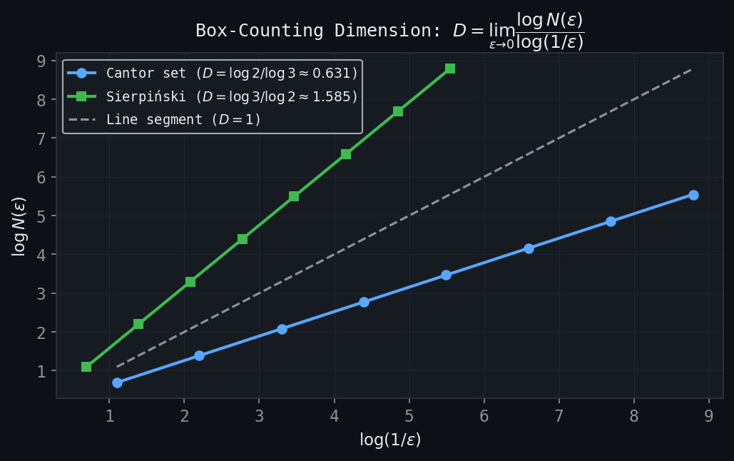Figure: Log-log plots of \(N(\varepsilon)\) vs \(1/\varepsilon\). The slope equals the fractal dimension: \(\ln 2/\ln 3 \approx 0.631\) for the Cantor set and \(\ln 3/\ln 2 \approx 1.585\) for the Sierpinski triangle.

For practical measurement of fractal dimension, one uses the box-counting dimension (also called the Minkowski-Bouligand dimension). Cover the set \( A \) with a grid of \( \varepsilon \)-boxes (squares in \( \mathbb{R}^2 \), cubes in \( \mathbb{R}^3 \)), and let \( N(\varepsilon) \) be the number of boxes that intersect \( A \). The box-counting dimension is

\[ D = \lim_{\varepsilon \to 0} \frac{\log N(\varepsilon)}{\log(1/\varepsilon)}, \]

provided the limit exists. In practice, one plots \( \log N(\varepsilon) \) versus \( \log(1/\varepsilon) \) for several values of \( \varepsilon \) and estimates \( D \) from the slope of the best-fit line.

Experimental measurements using box-counting yield:

• Sierpinski gasket (physical construction): \( D \approx 1.586 \).
• Mouse ear vasculature (branching blood vessels): \( D \approx 1.16 \) to \( 1.64 \), depending on the region.

These measurements demonstrate that natural biological structures can have non-integer dimensions, reflecting the self-similar branching patterns found in biological systems shaped by optimization and growth processes.

Fractals in Nature

The presence of fractal geometry in nature is not coincidental. Fractal branching patterns optimize the surface area available for exchange (lungs, villi), the reach of distribution networks (vasculature, river systems), and the efficiency of space-filling. A fractal tree, for example, maximizes the total leaf area within a finite volume. The fractal dimension of these structures quantifies how efficiently they fill space: a lung with branching dimension close to 3 is a more complete space-filler than one with dimension close to 2. The study of fractal geometry in nature connects the abstract mathematics of self-similarity to fundamental questions in physiology, ecology, and geomorphology.

---

Chapter 12: Iterated Function Systems

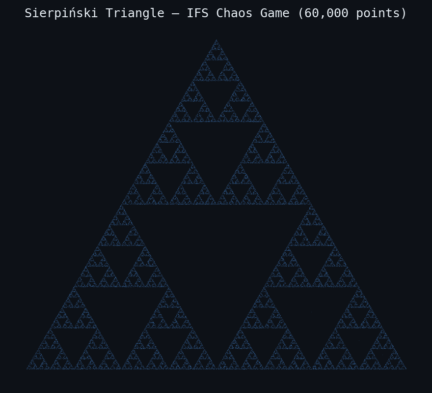Figure: The Sierpinski triangle rendered via 60,000 random IFS iterations (chaos game).

Attractors from Contractions

The preceding chapters have shown that fractals like the Cantor set and the von Koch curve can be constructed by repeated geometric operations — removing intervals, replacing segments with bent curves, and so on. Iterated Function Systems (IFS) provide a unified algebraic framework for this construction and for a much wider class of fractals, including Barnsley’s famous fern.

Figure: The Barnsley fern — attractor of a 4-map affine IFS, computed via 100,000 random iterations.

Contraction Mappings

The theoretical foundation rests on the concept of a contraction mapping.

Definition of an IFS

The Hausdorff metric \( h(A, B) \) measures the distance between two compact sets: it is the smallest \( \varepsilon \) such that \( A \subseteq B_\varepsilon(B) \) and \( B \subseteq B_\varepsilon(A) \).

The Cantor Set as an IFS Attractor

The ternary Cantor set \( C \) is the attractor of the two-map IFS:

\[ f_1(x) = \frac{x}{3}, \qquad f_2(x) = \frac{x}{3} + \frac{2}{3}. \]

One verifies that \( C = f_1(C) \cup f_2(C) \): the map \( f_1 \) maps \( C \) onto the left third of \( C \), and \( f_2 \) maps it onto the right third. Starting from \( S_0 = [0,1] \), after one application: \( S_1 = [0, 1/3] \cup [2/3, 1] \), which is exactly \( C_1 \) in the classical construction. Subsequent applications remove middle thirds iteratively, recovering the standard Cantor set construction. The dimension of this IFS attractor satisfies the Moran equation \( (1/3)^D + (1/3)^D = 1 \), giving \( D = \log 2 / \log 3 \) as expected.

Examples of IFS Attractors

The real power of IFS becomes apparent through a variety of examples.

The von Koch Curve is the attractor of a 4-map IFS on \( \mathbb{R}^2 \), where each map is a similarity that contracts by factor \( 1/3 \) and includes appropriate rotations to arrange the four pieces in the characteristic von Koch pattern.

Sierpinski Triangle (Gasket). Three maps on \( \mathbb{R}^2 \), each contracting by factor \( 1/2 \) toward one vertex of an equilateral triangle:

\[ f_i(\mathbf{x}) = \frac{1}{2}(\mathbf{x} - \mathbf{v}_i) + \mathbf{v}_i = \frac{1}{2}\mathbf{x} + \frac{1}{2}\mathbf{v}_i, \quad i = 1, 2, 3. \]

The attractor is the Sierpinski triangle with dimension \( D = \log 3 / \log 2 \approx 1.585 \).

Modified Sierpinski Gaskets. By introducing rotations and reflections into the component maps, one can create variations: the Cantor tree (maps along a line with rotations), Cantor dust (two non-collinear maps in the plane), and other variants. These demonstrate that the IFS framework is remarkably flexible: small changes in the contraction maps produce qualitatively different attractors.

The Twin Dragon. A two-map IFS in the complex plane using specific rotational contractions generates the twin dragon curve, a fractal with a characteristic winged shape that tiles the plane.

Tree-like IFS. An IFS with two maps — one map pointing “up” at a slight lean, the other pointing “up” at the opposite lean — produces a fractal tree-like structure. More elaborate trees arise by using several branches with different angles and contraction ratios.

Barnsley’s Fern. Perhaps the most famous IFS is Barnsley’s spleenwort fern, defined by four affine maps on \( \mathbb{R}^2 \):

\[ f_1(\mathbf{x}) = \begin{pmatrix} 0 \\ 0.16 y \end{pmatrix}, \quad f_2(\mathbf{x}) = \begin{pmatrix} 0.85x + 0.04y \\ -0.04x + 0.85y + 1.6 \end{pmatrix}, \]\[ f_3(\mathbf{x}) = \begin{pmatrix} 0.2x - 0.26y \\ 0.23x + 0.22y + 1.6 \end{pmatrix}, \quad f_4(\mathbf{x}) = \begin{pmatrix} -0.15x + 0.28y \\ 0.26x + 0.24y + 0.44 \end{pmatrix}. \]

The attractor of this four-map IFS is a faithful model of a Nephrolepis exaltata fern frond. Map \( f_1 \) maps the entire fern to a short stalk; map \( f_2 \) produces the large central frond; maps \( f_3 \) and \( f_4 \) produce the lowest two leaflets. The result is visually indistinguishable from a real fern, demonstrating that biological shapes can arise from iterative self-similar processes.

Computing IFS Attractors: The Random Iteration Algorithm

There are two practical algorithms for visualizing IFS attractors.

The Deterministic Algorithm

Start with any compact set \( S_0 \) (a single point suffices) and compute \( S_{n+1} = \hat{f}(S_n) \) iteratively. After \( n \) steps, \( S_n \) contains (in principle) \( N^n \) points. In practice, computing and storing \( N^n \) points becomes infeasible for large \( n \), so this method is most useful for small systems or analytical studies.

The Random Iteration Algorithm (Chaos Game)

The random iteration algorithm, also called the chaos game, is far more efficient. Choose an initial point \( x_0 \in X \). At each step, select one of the \( N \) maps \( f_i \) randomly with probability \( p_i \) (where \( \sum p_i = 1 \)) and apply it: \( x_{n+1} = f_{\sigma_n}(x_n) \). The orbit \( \{x_n\}_{n \geq 0} \) is a random sequence that, with probability 1, becomes dense in the attractor \( A \). Plotting the orbit after a short transient reveals the shape of \( A \).

The probabilities \( p_i \) can be chosen proportional to the area scaling of each map (\( p_i \propto |\det J_{f_i}| \)), which gives a visually uniform density. For Barnsley’s fern, the probabilities are \( p_1 = 0.01 \), \( p_2 = 0.85 \), \( p_3 = 0.07 \), \( p_4 = 0.07 \), corresponding to the relative sizes of the parts of the fern. The random iteration algorithm converges rapidly: just a few thousand iterates suffice to give a convincing picture.

The Inverse Problem: Collage Theorem

Given an attractor and wishing to find the IFS that generates it, one uses the following heuristic.

The Collage Theorem says: to find an IFS whose attractor approximates \( S \), find maps \( f_i \) such that the collage \( \hat{f}(S) = f_1(S) \cup \cdots \cup f_N(S) \) closely covers \( S \). In practice, one overlays copies of \( S \) onto \( S \) itself, using scaled, rotated, and translated versions, until the copies tile \( S \) with small residual. The contraction maps corresponding to these overlays define the approximating IFS.

IFS with Grey-Level Maps (IFSM)

The IFS framework extends from attractors (sets) to functions via IFS with grey-level maps (IFSM). Here one specifies:

• A set of contraction maps \( f_1, \ldots, f_N \) on the base space.
• A corresponding set of grey-level maps (or shading functions) \( \phi_i : \mathbb{R} \to \mathbb{R} \), often of the form \( \phi_i(y) = \alpha_i y + \beta_i \).

The IFSM defines an operator \( T \) acting on bounded functions \( u : X \to \mathbb{R} \) by

\[ (Tu)(x) = \sum_{i : x \in f_i(X)} \phi_i(u(f_i^{-1}(x))). \]

Under appropriate contractivity conditions on the \( \phi_i \) (specifically, \( \sum |\alpha_i| < 1 \)), the operator \( T \) is a contraction on the space of bounded functions, and its unique fixed point \( \bar{u} = T\bar{u} \) is the attractor function of the IFSM.

The Devil’s Staircase

A canonical example of an IFSM attractor is the Devil’s Staircase (Cantor function). Consider a three-map IFSM on \( [0,1] \):

\[ f_1(x) = \frac{x}{3}, \quad f_2(x) = \frac{x}{3} + \frac{1}{3}, \quad f_3(x) = \frac{x}{3} + \frac{2}{3}, \]

with grey-level maps \( \phi_1(y) = y/2 \), \( \phi_2(y) = 1/2 \) (constant), \( \phi_3(y) = y/2 + 1/2 \). The attractor function \( \bar{u} \) is the Devil’s Staircase: a continuous, non-decreasing function on \( [0,1] \) that is constant on the removed intervals of the Cantor set and increases only on the Cantor set itself, which has measure zero. Its derivative is zero almost everywhere, yet it rises from 0 to 1. The Devil’s Staircase is a striking example of a function that is continuous but not absolutely continuous.

Fractal Image Coding

The IFSM framework provides the theoretical basis for fractal image compression (Barnsley and Hurd, 1992; Jacquin, 1992). A grey-scale image is represented as a function \( u : [0,1]^2 \to [0,1] \), where \( u(x,y) \) gives the brightness at pixel \( (x,y) \). The image is encoded by finding an IFSM operator \( T \) such that \( Tu \approx u \), i.e., the image is (approximately) a fixed point of \( T \).

In practice, the domain of the image is partitioned into range blocks \( R_i \) (small, non-overlapping tiles) and domain blocks \( D_j \) (larger tiles, possibly overlapping, from the same image). For each range block \( R_i \), one finds the domain block \( D_j \) that, after decimation (shrinking to the size of \( R_i \)) and a grey-level affine map \( \phi(y) = \alpha y + \beta \), best approximates \( R_i \) in least-squares sense. The optimal \( \alpha \) and \( \beta \) for each pair \( (R_i, D_j) \) are found by minimizing

\[ \| \phi(\text{decimated } D_j) - R_i \|^2. \]

The encoded image is then just the list of triplets \( (i, j, \alpha_i, \beta_i) \) — a compact representation from which the original image can be reconstructed (approximately) by iterating \( T \) from any starting function. Fractal image coding can achieve high compression ratios with good visual quality, particularly for images with self-similar structure at different scales (natural scenes, textures). The decoding is computationally fast (just iterate \( T \)); the encoding (searching for matching domain blocks) can be slow but needs to be done only once.

---

These notes are based on the AMATH 343 lectures by Professor E.R. Vrscay, University of Waterloo, Fall 2021. All mathematical content is drawn from the course materials; any errors in transcription or synthesis are the responsibility of the note-taker.