PMATH 464: Introduction to Algebraic Geometry

David McKinnon

Estimated study time: 1 hr 41 min

Table of contents

L’algèbre n’est qu’une géométrie écrite, la géométrie n’est qu’une algèbre figurée. — Sophie Germain

These notes are based on Prof. David McKinnon’s lectures, enriched with material from Prof. S. New’s PMATH 464/764 lecture notes.

Algebraic Sets

1. What is Algebraic Geometry?

Sophie Germain had it right: algebra is written geometry, and geometry is algebra in pictures. The great thing about geometry is that it is full of pictures — there is a physicality to it that makes it easier to guess what is going on, to guide one’s intuition. Trouble is, it is often fiendishly difficult to actually prove that intuition. The pictures that so eloquently inspire you to understand the truth also conspire to conceal nuances and special cases.

Algebra, unlike geometry, is quite amenable to computation — that is kind of the whole point of it. But algebra and intuition are not good friends. Look at an algebraic statement, and it is often hard to understand what it is all about.

Enter the genius of Germain. If you can somehow marry the two subjects of algebra and geometry, then you can get the best of both worlds: the intuition of geometry, and the calculational power of algebra. The key is functions. If you have a Geometry Thing, then the corresponding Algebra Thing is the set of functions from the Geometry Thing to some nice algebra place, like the complex numbers.

In this course, we will be working over the complex numbers, and all the algebra we do will be with polynomials (and closely related beasts). The Geometry Things we talk about are also defined by polynomials.

2. Algebraic Sets

Affine variety V(y − x²): parabola in affine plane A²

Definition 2.1. Let \(n\) be a positive integer. Affine space \(\mathbb{A}^n\) is the set \(\mathbb{C}^n\).

Definition 2.2. Let \(S\) be a subset of the polynomial ring \(\mathbb{C}[x_1, \ldots, x_n]\). The algebraic set corresponding to \(S\) is: \[ V(S) = \{ x \in \mathbb{A}^n \mid f(x) = 0 \text{ for all } f \in S \} \] In other words, \(V(S)\) is the set of points where all functions in \(S\) vanish.

There are lots of algebraic sets. The \(xy\)-plane is the algebraic subset of \(\mathbb{A}^2\) corresponding to the empty set \(S\). The \(x\)-axis is \(V(\{y\})\). The unit “sphere” in \(\mathbb{C}^3\) is \(V(x^2 + y^2 + z^2 - 1)\). The twisted cubic is the algebraic subset of \(\mathbb{A}^3\) defined by \(\{y - x^2, z - x^3\}\). The origin in \(\mathbb{A}^2\) is defined by \(\{x, y\}\).

Although we work over \(\mathbb{C}\) in this course, the definition makes sense over any field \(F\). Working over different fields produces strikingly different geometry from the same equations. Over \(\mathbb{R}\), the circle \(V(x^2 + y^2 - 1)\) is the familiar unit circle, while \(V(x^2 + y^2 + 1) = \varnothing\) — there are no real solutions. Over \(\mathbb{C}\), neither equation produces an empty variety (a consequence of the Nullstellensatz). Over finite fields, every variety is a finite set of points: in \(\mathbb{Z}_3^2\), the “circle” \(V(x^2 + y^2 - 1)\) consists of just four points \(\{(0,1), (0,2), (1,0), (2,0)\}\).

The classification of varieties in one variable is simple but instructive: in \(F^1\), every variety is either \(F\) itself (when \(S = \varnothing\)), the empty set (when \(S\) contains a nonzero constant), or a finite set of points (since a nonzero polynomial has finitely many roots). In higher dimensions, the picture becomes richer. In \(F^2\), we can form unions: for instance, \(V\bigl((x-a)(x-c), (x-a)(y-d), (x-c)(y-b), (y-b)(y-d)\bigr)\) gives the two-point set \(\{(a,b), (c,d)\}\). And in \(F^{n^2}\), the set \(\operatorname{GL}(n,F)\) of invertible matrices is open in the Zariski topology — it is the complement of \(V(\det)\), the vanishing locus of the determinant polynomial.

This lets us make a Geometric Thing out of an Algebra Thing. Next step: go the other way.

Definition 2.3. Let \(X \subset \mathbb{A}^n\) be a subset of affine space. The ideal of \(X\) is: \[ I(X) = \{ f \in \mathbb{C}[x_1, \ldots, x_n] \mid f(P) = 0 \text{ for all } P \in X \} \]

The ideal of the \(x\)-axis is \((y)\), since the vanishing polynomials are exactly those you can factor a \(y\) out of. The ideal of the origin is \((x, y)\).

Theorem 2.4. Let \(X\) be a subset of \(\mathbb{A}^n\), and \(I(X)\) its ideal. Then \(I(X)\) is a radical ideal of \(\mathbb{C}[x_1, \ldots, x_n]\): if \(f^n \in I(X)\) for some positive integer \(n\), then \(f \in I(X)\).

Proof. For additivity: if \(f, g \in I(X)\) then \(f(x) = g(x) = 0\) for all \(x \in X\), so \((f \pm g)(x) = 0\) too. For multiplication: if \(h \in \mathbb{C}[x_1,\ldots,x_n]\) and \(f \in I(X)\), then \((hf)(x) = h(x) \cdot 0 = 0\). For radical: if \(f^n \in I(X)\), then \((f(x))^n = 0\) for all \(x \in X\), so \(f(x) = 0\), so \(f \in I(X)\). ∎

This means not every ideal is the ideal of an algebraic set — only radical ideals are. The finiteness of the algebraic world rests on a foundational result.

Definition 2.4a. A ring \(R\) is Noetherian if every ascending chain of ideals \(A_1 \subseteq A_2 \subseteq A_3 \subseteq \cdots\) eventually stabilizes: there exists an index \(\ell\) such that \(A_k = A_\ell\) for all \(k \geq \ell\). Equivalently, \(R\) is Noetherian if and only if every ideal of \(R\) is finitely generated.

The equivalence is easy to see: if every ideal is finitely generated, take \(A = \bigcup A_i\); its generators all lie in some \(A_\ell\), forcing the chain to stabilize. Conversely, if some ideal \(A\) were not finitely generated, we could build a strictly ascending chain by adding one generator at a time.

Theorem 2.4b (Hilbert's Basis Theorem). If \(R\) is Noetherian, then so is \(R[x]\). In particular, \(\mathbb{C}[x_1, \ldots, x_n]\) is Noetherian.

Proof. Let \(A\) be an ideal in \(R[x]\). For each \(k \geq 0\), let \(A_k\) be the set of leading coefficients of polynomials in \(A\) of degree \(k\), together with \(0\). Each \(A_k\) is an ideal in \(R\), and \(A_0 \subseteq A_1 \subseteq A_2 \subseteq \cdots\). Since \(R\) is Noetherian, this chain stabilizes at some index \(m\), meaning \(A_k = A_m\) for all \(k \geq m\). Each \(A_k\) is finitely generated: say \(A_k = (a_{k,1}, \ldots, a_{k,\ell_k})\). For each generator \(a_{k,i}\), choose a polynomial \(f_{k,i} \in A\) of degree \(k\) with leading coefficient \(a_{k,i}\).

Let \(B = (f_{k,i} \mid k \leq m,\, i \leq \ell_k)\). We claim \(A = B\). If \(f \in A\) has degree \(k \leq m\), its leading coefficient lies in \(A_k\), so we can subtract a suitable linear combination of the \(f_{k,i}\) to reduce the degree. If \(\deg f = k > m\), the leading coefficient lies in \(A_k = A_m\), so we multiply the \(f_{m,i}\) by \(x^{k-m}\) and subtract to reduce the degree. By induction on degree, every \(f \in A\) lies in \(B\). ∎

Since \(\mathbb{C}\) is a field (hence Noetherian), repeated application gives that \(\mathbb{C}[x_1, \ldots, x_n]\) is Noetherian. Thus every algebraic set is defined by finitely many polynomials.

Definition 2.5. An ideal \(I\) of a ring \(R\) is called radical if every \(r \in R\) with \(r^n \in I\) for some positive integer \(n\) satisfies \(r \in I\). For an arbitrary ideal \(I\), define the radical of \(I\) to be: \[ \text{rad}(I) = \{ r \in R \mid r^n \in I \text{ for some integer } n > 0 \} \]

Theorem 2.6. Let \(I\) be an ideal of a ring \(R\). Then \(\text{rad}(I)\) is a radical ideal of \(R\) containing \(I\).

Proof sketch. Clearly \(I \subseteq \text{rad}(I)\) (take \(n = 1\). For closure under multiplication: if \(j \in \text{rad}(I)\) with \(j^n \in I\), then \((rj)^n = r^n j^n \in I\). For radical: if \(j^n \in \text{rad}(I)\), then \((j^n)^m \in I\), so \(j^{nm} \in I\). For closure under addition: if \(j_1^{n_1} \in I\) and \(j_2^{n_2} \in I\), then every term of \((j_1 \pm j_2)^{n_1 + n_2}\) contains either a factor of \(j_1^{n_1}\) or \(j_2^{n_2}\), so \((j_1 \pm j_2)^{n_1+n_2} \in I\). ∎

We are now ready for the big correspondence — the theorem that makes the entire subject work. Its proof requires the machinery of Noether normalization (developed later in these notes), but we state it here because it governs every construction that follows.

Theorem 2.7 (Hilbert's Weak Nullstellensatz). Let \(A \subsetneq \mathbb{C}[x_1, \ldots, x_n]\) be a proper ideal. Then \(V(A) \neq \varnothing\).

Proof. Choose a maximal ideal \(M\) containing \(A\) (by Zorn's lemma). Then \(L = \mathbb{C}[x_1, \ldots, x_n]/M\) is a field containing \(\mathbb{C}\). Writing \(u_i = x_i + M\), we have \(L = \mathbb{C}[u_1, \ldots, u_n]\). If some \(u_i\) were transcendental over \(\mathbb{C}\), then by Noether normalization, \(L\) would contain a polynomial subring over which it is integral, and the Lying Over Theorem would force a nontrivial maximal ideal in \(L\) — impossible since \(L\) is a field and \(\{0\}\) is its only maximal ideal. So every \(u_i\) is algebraic over \(\mathbb{C}\), hence \(u_i \in \mathbb{C}\) (since \(\mathbb{C}\) is algebraically closed). Choosing \(a_i \in \mathbb{C}\) with \(u_i = a_i + M\), the point \(a = (a_1, \ldots, a_n)\) lies in \(V(M) \subseteq V(A)\). ∎

Theorem 2.7a (Hilbert's Strong Nullstellensatz). Let \(A\) be an ideal in \(\mathbb{C}[x_1, \ldots, x_n]\). Then \(I(V(A)) = \sqrt{A}\). In particular, there is a bijection: \[ \{\text{algebraic subsets of } \mathbb{A}^n\} \longleftrightarrow \{\text{radical ideals of } \mathbb{C}[x_1, \ldots, x_n]\} \] given by \(X \mapsto I(X)\) and \(I \mapsto V(I)\).

Proof (Rabinowitsch trick). We always have \(\sqrt{A} \subseteq I(V(A))\), so take \(f \in I(V(A))\). Introduce a new variable \(y\) and let \(B = (A, yf - 1) \subseteq \mathbb{C}[x_1, \ldots, x_n, y]\). If \((a, b) \in V(B)\), then \(a \in V(A)\), so \(f(a) = 0\), but also \(bf(a) = 1\) — a contradiction. So \(V(B) = \varnothing\), and by the Weak Nullstellensatz, \(B = \mathbb{C}[x_1, \ldots, x_n, y]\). In particular, \(1 \in B\): \[ 1 = \sum_{i=1}^{k} f_i(x,y) g_i(x,y) + (yf(x) - 1) g_{k+1}(x,y) \] with \(f_i \in A\). Setting \(y = 1/f(x)\) in the fraction field \(\mathbb{C}(x_1, \ldots, x_n)\) and clearing denominators by multiplying by \(f^N\) (where \(N\) is the highest power of \(y\) appearing), we obtain \(f^N \in A\). Hence \(f \in \sqrt{A}\). ∎

This correspondence is more awesome than it appears. Under it:

Bigger ideals correspond to smaller algebraic sets: \(X \subset Y\) if and only if \(I(Y) \subset I(X)\).
Unions of algebraic sets correspond to intersections of ideals: \(I(X \cup Y) = I(X) \cap I(Y)\).
Maximal ideals correspond to single points: \(I(X)\) is maximal if and only if \(X\) is a single point. (The key insight is the evaluation homomorphism \(\phi: \mathbb{C}[x_1,\ldots,x_n] \to \mathbb{C}\) defined by \(\phi(f) = f(P)\), which is surjective with kernel \(I(P)\).)
Prime ideals correspond to irreducible algebraic sets.

Definition 2.8. Let \(X\) be a nonempty algebraic set. We say that \(X\) is reducible if and only if it is the union \(X = Y_1 \cup Y_2\) of two proper algebraic subsets. We say that \(X\) is irreducible if and only if it is not reducible. (The empty set is neither irreducible nor reducible.)

The proof of the correspondence between prime ideals and irreducible sets is elegant: if \(I(X)\) is not prime, there exist polynomials \(f_1, f_2 \notin I(X)\) with \(f_1 f_2 \in I(X)\). Then \(X = (X \cap V(f_1)) \cup (X \cap V(f_2))\) is a decomposition into proper algebraic subsets. Conversely, if \(X = Y \cup Z\) with \(Y, Z \subsetneq X\), choose \(f \in I(Y) \setminus I(X)\) and \(g \in I(Z) \setminus I(X)\). Then \(fg\) vanishes on \(Y \cup Z = X\), so \(fg \in I(X)\) with neither factor in \(I(X)\) — the ideal is not prime.

Every algebraic set breaks into irreducible pieces, and this decomposition is essentially unique.

Theorem 2.9 (Irreducible Decomposition). Every nonempty algebraic set \(X\) can be written as a finite union \(X = X_1 \cup \cdots \cup X_r\) of irreducible algebraic sets, with no \(X_i\) contained in any \(X_j\) for \(i \neq j\). This decomposition is unique up to reordering.

Proof. Existence: If \(X\) is irreducible, we are done. Otherwise \(X = Y_1 \cup Z_1\) with \(Y_1, Z_1 \subsetneq X\). If \(Z_1\) is irreducible, stop; otherwise decompose \(Z_1 = Y_2 \cup Z_2\), giving \(X = Y_1 \cup Y_2 \cup Z_2\). This process must terminate: an infinite chain \(Z_1 \supsetneq Z_2 \supsetneq \cdots\) would produce an infinite ascending chain \(I(Z_1) \subsetneq I(Z_2) \subsetneq \cdots\) of ideals, contradicting the Noetherian property. Discard any \(X_i\) contained in another \(X_j\) to obtain the minimal decomposition.

Uniqueness: Suppose \(X = X_1 \cup \cdots \cup X_r = Y_1 \cup \cdots \cup Y_s\). Fix \(i\). Then \(X_i = (Y_1 \cap X_i) \cup \cdots \cup (Y_s \cap X_i)\). Since \(X_i\) is irreducible, \(X_i = Y_j \cap X_i\) for some \(j\), giving \(X_i \subseteq Y_j\). By symmetry, \(Y_j \subseteq X_k\) for some \(k\), so \(X_i \subseteq X_k\), forcing \(i = k\) and hence \(X_i = Y_j\). ∎

For varieties in the affine plane, the story has a particularly clean ending.

Theorem 2.10 (Classification in \(\mathbb{A}^2\)). Let \(F\) be an infinite field. Then:

If \(f, g \in F[x,y]\) share no common factor, then \(V(f) \cap V(g)\) is finite.
If \(f\) is irreducible and \(V(f)\) is infinite, then \(V(f)\) is irreducible with \(I(V(f)) = (f)\).
The irreducible varieties in \(F^2\) are: single points, infinite sets \(V(f)\) for irreducible \(f\), and \(F^2\) itself.

The key to part (1) is the Euclidean algorithm: since \(f\) and \(g\) have no common factor in \(F[x][y]\), we can find \(s, t \in F(x)[y]\) with \(fs + gt = 1\), and clearing denominators yields \(fp + gq = r(x)\) for some nonzero \(r \in F[x]\). Any common zero of \(f\) and \(g\) must be a root of \(r(x)\), of which there are finitely many. Part (2) follows: if \(g \in I(V(f))\), then \(V(f) \cap V(g) = V(f)\) is infinite, so \(f\) and \(g\) share a factor — which must be \(f\) itself, giving \(g \in (f)\).

Affine Maps and Equivalence

Before we develop the full theory of polynomial maps, it is worth pausing to consider the simplest kind of map between varieties: affine maps, which combine a linear transformation with a translation.

Definition 3.1. An affine map from \(\mathbb{A}^n\) to \(\mathbb{A}^m\) is a function \(f(x) = Ax + b\) for some \(m \times n\) matrix \(A\) and vector \(b \in \mathbb{A}^m\). An affine equivalence (or affine change of coordinates) is a bijective affine map \(f : \mathbb{A}^n \to \mathbb{A}^n\), which requires \(n = m\) and \(A\) invertible.

Two algebraic sets \(X \subseteq \mathbb{A}^n\) and \(Y \subseteq \mathbb{A}^m\) are affinely equivalent if there is an affine map \(f : \mathbb{A}^n \to \mathbb{A}^m\) restricting to a bijection \(f : X \to Y\) whose inverse is also affine. Affine equivalence is a coarse but useful notion: it tells us when two varieties are “the same” up to a change of coordinates. For affine subspaces, the classification is immediate — two affine subspaces are equivalent if and only if they have the same dimension.

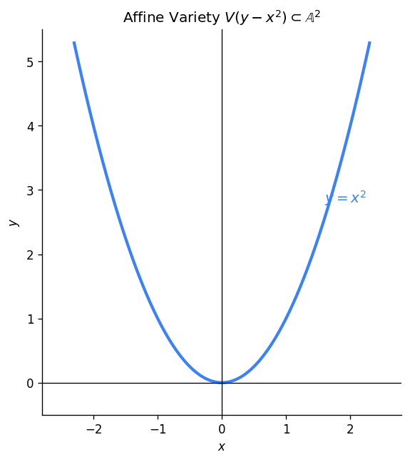
The classification of plane conics illustrates the power of affine equivalence. By diagonalizing the associated symmetric bilinear form (and applying Sylvester’s Law of Inertia over \(\mathbb{R}\)), one shows that every degree-2 variety \(V(f) \subseteq \mathbb{R}^2\) is affinely equivalent to one of: the circle \(V(x^2 + y^2 - 1)\), the hyperbola \(V(x^2 - y^2 - 1)\), the parabola \(V(y - x^2)\), a pair of intersecting lines \(V(x^2 - y^2)\), parallel lines \(V(y^2 - 1)\), a single line \(V(y^2)\), a point \(V(x^2 + y^2)\), or the empty set \(V(x^2 + y^2 + 1)\).

Over \(\mathbb{C}\), the classification collapses: the circle and hyperbola become equivalent (via \((x,y) \mapsto (ix, y)\)), leaving only the circle \(V(x^2 + y^2 - 1)\), the parabola \(V(y - x^2)\), intersecting lines \(V(x^2 - y^2)\), and a single line \(V(y^2)\). The “missing” cases — the point, the empty set, parallel lines — all merge into existing classes because \(\mathbb{C}\) has enough square roots and algebraic solutions.

Polynomial Maps and Coordinate Rings

1. Morphisms

These days, every time mathematicians start a new subject, they define the objects they are interested in, and then immediately define the relationships between them. For algebraic sets, those relationships are functions that preserve their algebraic structure.

Definition 1.1. Let \(X \subset \mathbb{A}^n\) and \(Y \subset \mathbb{A}^m\) be algebraic sets. A polynomial map from \(X\) to \(Y\) is a function \(\phi : X \to Y\) such that the coordinates of \(\phi = (\phi_1, \ldots, \phi_m)\) are all polynomials in the coordinates of \(\mathbb{A}^n\).

For example, \(\phi : \mathbb{A}^1 \to \mathbb{A}^3\) given by \(\phi(t) = (t, t^2, t^3)\) is a polynomial map (parametrizing the twisted cubic). The map \(\phi : H \to C\) given by \(\phi(x,y) = (x, iy)\) from the hyperbola \(H: x^2 - y^2 = 1\) to the circle \(C: x^2 + y^2 = 1\) is a polynomial map — with polynomial inverse \(\psi(x,y) = (x, -iy)\) — and so it is an isomorphism.

Definition 1.2. A polynomial map \(f : X \to Y\) is an isomorphism if there is a polynomial map \(g : Y \to X\) such that \(f \circ g = \text{id}\) and \(g \circ f = \text{id}\).

Warning: a polynomial map that is one-to-one and onto is not necessarily an isomorphism — you also need the inverse to be a polynomial map.

2. Coordinate Rings

The ideal of an algebraic set is not invariant under isomorphism. For example, the \(x\)-axis in \(\mathbb{A}^2\) has ideal \((y)\), while the \(x\)-axis in \(\mathbb{A}^3\) has ideal \((y, z)\) — but these are clearly isomorphic algebraic sets. We need something better.

Definition 1.3. Let \(X \subset \mathbb{A}^n\) be an algebraic set with ideal \(I(X)\). The coordinate ring of \(X\) is the ring: \[ \Gamma(X) = \mathbb{C}[x_1, \ldots, x_n] / I(X) \] which is the ring of polynomial maps from \(X\) to \(\mathbb{A}^1\).

Why is \(\Gamma(X)\) the ring of polynomial maps from \(X\) to \(\mathbb{A}^1\)? Because \(f\) and \(g\) agree on \(X\) if and only if \(f - g\) vanishes on \(X\), i.e., \(f \equiv g \pmod{I(X)}\).

The Nullstellensatz correspondence still works for coordinate rings:

Theorem 1.4. There is a bijection between algebraic subsets of \(X\) and radical ideals of \(\Gamma(X)\). Under this correspondence, points correspond to maximal ideals, and irreducible subsets correspond to prime ideals.

3. Pullbacks

Given a polynomial map \(\phi : X \to Y\), we can turn it into a homomorphism going backwards. If someone hands us a polynomial map \(f : Y \to \mathbb{A}^1\), we can compose to get \(f \circ \phi : X \to \mathbb{A}^1\).

Definition 1.5. Let \(X\) and \(Y\) be rings containing \(\mathbb{C}\) (called \(\mathbb{C}\)-algebras). A \(\mathbb{C}\)-algebra homomorphism is a ring homomorphism \(\phi : X \to Y\) satisfying \(\phi(z) = z\) for all \(z \in \mathbb{C}\).

Definition 1.6. Let \(\phi : X \to Y\) be a polynomial map of algebraic sets. The pullback of \(\phi\) is the \(\mathbb{C}\)-algebra homomorphism: \[ \phi^* : \Gamma(Y) \to \Gamma(X) \quad \text{given by} \quad \phi^*(f) = f \circ \phi \]

Theorem 1.7. For any \(\mathbb{C}\)-algebra homomorphism \(\psi : \Gamma(Y) \to \Gamma(X)\), there is a polynomial map \(\phi : X \to Y\) such that \(\psi = \phi^*\).

Proof sketch. Say \(X \subset \mathbb{A}^n\) and \(Y \subset \mathbb{A}^m\). To build \(\phi\), we need \(m\) polynomials. The \(i\)th coordinate function on \(Y\) is just \(x_i\), so set \(\phi_i\) to be any polynomial representative of \(\psi(x_i) \in \Gamma(X)\). Define \(\phi(P) = (\phi_1(P), \ldots, \phi_m(P))\). One then verifies that \(\phi^*(I(Y)) \subset I(X)\), so \(\phi\) maps \(X\) to \(Y\), and that \(\phi^* = \psi\). ∎

Theorem 1.8. Let \(X\) and \(Y\) be algebraic sets. Then \(X \cong Y\) if and only if \(\Gamma(X) \cong \Gamma(Y)\) as \(\mathbb{C}\)-algebras. Moreover, if \(\phi : X \to Y\) is an isomorphism and \(V \subset Y\) is any algebraic subset, then \(I(\phi^{-1}(V)) = \phi^* I(V)\).

This is the coup de grâce: two algebraic sets are isomorphic if and only if their coordinate rings are isomorphic as \(\mathbb{C}\)-algebras.

4. Dominance and the Image of a Polynomial Map

A polynomial map need not be surjective, and its image need not even be an algebraic set. The map \(f : V(xy - 1) \to \mathbb{A}^1\) given by \(f(x,y) = x\) has image \(\mathbb{A}^1 \setminus \{0\}\), which is not a variety. The right notion is dominance: \(f\) is dense enough.

Definition 1.9. A polynomial map \(f : X \to Y\) is dominant if \(\overline{f(X)} = Y\) (the image is dense in the Zariski topology). It has a left polynomial inverse if there exists \(g : Y \to X\) with \(g \circ f = \operatorname{id}_X\).

Theorem 1.10. Let \(f : X \to Y\) be a polynomial map. Then:

\(f^*\) is injective if and only if \(f\) is dominant.
\(f^*\) is surjective if and only if \(f\) has a left polynomial inverse.

The first part captures a recurring theme: injectivity on the algebra side corresponds to surjectivity (or at least density) on the geometric side. The proof of (1) is direct: \(f^*\) injective means \(g \circ f = 0 \Rightarrow g = 0\) in \(\Gamma(Y)\), which says precisely that the only polynomial vanishing on \(f(X)\) is the zero class — i.e., \(I(f(X)) = I(Y)\), so \(\overline{f(X)} = Y\).

5. Non-Isomorphism via Coordinate Rings

The coordinate ring is a powerful invariant. It can prove that two varieties that look alike are genuinely different.

Example: The cuspidal cubic \(X = V(y^2 - x^3) \subseteq \mathbb{A}^2\) is not isomorphic to \(\mathbb{A}^1\). The map \(f : \mathbb{A}^1 \to X\) given by \(f(t) = (t^2, t^3)\) is surjective but not an isomorphism. To see why, note that \(f^* : \Gamma(X) \to \mathbb{C}[t]\) sends \(x \mapsto t^2\) and \(y \mapsto t^3\). The image \(f^*(\Gamma(X))\) is the subring of \(\mathbb{C}[t]\) generated by \(t^2\) and \(t^3\) — this contains \(t^4 = (t^2)^2, t^5 = t^2 \cdot t^3, t^6 = (t^3)^2\), and so on, but not \(t\) itself. In \(\Gamma(X)\), the elements \(x\) and \(y\) are both irreducible, yet \(x^3 = y^2\), so \(\Gamma(X)\) is not a UFD. Since \(\mathbb{C}[t]\) is a UFD, we have \(\Gamma(X) \not\cong \mathbb{C}[t]\), hence \(X \not\cong \mathbb{A}^1\).

Rational Functions and Local Rings

1. Varieties and Function Fields

So far, our algebra has been limited to addition, subtraction, and multiplication. Time to add division. Division works better in rings without zero divisors — and recall from last week that \(\Gamma(X)\) is a domain if and only if \(X\) is irreducible.

Moreover, every algebraic set is a finite union of irreducible algebraic sets (by the Noetherian property of \(\mathbb{C}[x_1, \ldots, x_n]\), and this decomposition is unique. This motivates a special name.

Definition 1.1. Let \(X = X_1 \cup \cdots \cup X_r\) be an expression of \(X\) as the union of finitely many irreducible algebraic subsets. The sets \(X_i\) are called the irreducible components of \(X\).

Definition 1.2. A variety is an irreducible algebraic set.

Definition 1.3. Let \(X\) be a variety. The function field \(K(X)\) of \(X\) is the fraction field of the coordinate ring \(\Gamma(X)\). An element of \(K(X)\) is called a rational function.

The function field of \(\mathbb{A}^n\) is \(\mathbb{C}(x_1, \ldots, x_n)\), the field of rational functions of \(n\) variables. In general, elements of \(K(X)\) are fractions of elements of \(\Gamma(X)\). These fractions are almost functions: they may fail to be defined at points where the denominator vanishes.

Definition 1.4. Let \(f\) be a rational function on a variety \(X\), and let \(P \in X\) be a point. Then \(f\) is defined at \(P\) if there is some expression \(f = p/q\) for \(p, q \in \Gamma(X)\) with \(q(P) \neq 0\). If \(f\) is not defined at \(P\), we say that \(P\) is a pole of \(f\).

A subtlety: even if one representation has a zero denominator, another might not. For example, on \(V(y^2 - x^3 + x)\), the function \(x/y\) appears to have a pole at \((0,0)\), but \(x/y = y/(x^2 - 1)\), which has a nonzero denominator at the origin.

Theorem 1.5. If \(f = p/q\) with \(q(P) = 0\) and \(p(P) \neq 0\), then \(P\) is a pole of \(f\).

Proof. For any representation \(f = a/b\), we have \(aq = bp\). Since \(q(P) = 0\), we get \((bp)(P) = 0\), and since \(p(P) \neq 0\), this forces \(b(P) = 0\). So every representation of \(f\) has a vanishing denominator at \(P\). ∎

2. Local Rings

Definition 1.6. Let \(X\) be a variety, \(P \in X\). The local ring at \(P\) is: \[ \mathcal{O}_P(X) = \{ f \in K(X) \mid f \text{ is defined at } P \} \] Its maximal ideal is \(\mathfrak{m}_P(X) = \{ f \in \mathcal{O}_P(X) \mid f(P) = 0 \}\), and we have \(\mathfrak{m}_P(X) = I(P) \cdot \mathcal{O}_P(X)\).

The local ring captures all the information about a variety near a particular point, filtering out global concerns.

Rational Maps and the Zariski Topology

1. The Zariski Topology

Definition 0.1. Let \(V\) be an algebraic variety. A Zariski closed subset of \(V\) is an algebraic subset of \(V\). A subset \(U \subset V\) is Zariski open if \(V - U\) is Zariski closed.

The Zariski topology is named after Oscar Zariski, the great Russian-American mathematician who helped found algebraic geometry as a rigorous subject. Beware: it is a truly terrible topology, very far from Hausdorff. If two Zariski open sets are disjoint, then at least one of them is empty!

2. Rational Maps

Definition 0.2. Let \(V\) and \(W\) be varieties. A rational map from \(V\) to \(W\) is a function \(f : U \to W\) for some nonempty Zariski open subset \(U \subset V\), such that for every point \(P \in U\), there are rational functions \(f_1, \ldots, f_r\) on \(V\), all defined at \(P\), with \(f(Q) = (f_1(Q), \ldots, f_r(Q))\) for all \(Q\) where these are defined. We write \(f : V \dashrightarrow W\) for rational maps.

A rational map is a morphism on \(V' \subset V\) if it is defined at every point of \(V'\). Every polynomial map is a morphism. We will henceforth use “morphism” in place of “polynomial map”.

Definition 0.3. Let \(U \subset V\) be a Zariski open subset. The ring of functions on \(U\) is: \[ \Gamma(U) = \{ f \in K(V) \mid f \text{ has no poles in } U \} \]

Theorem 0.5. Let \(V\) be an affine variety, \(U \subset V\) a nonempty Zariski open subset. If \(U = V - V(f)\) for some \(f \in \Gamma(V)\), then: \[ \Gamma(U) = \Gamma(V)[1/f] = \{ p/f^r \mid r \in \mathbb{Z},\, p \in \Gamma(V) \} \]

An interesting consequence: for \(U = \mathbb{A}^2 - \{(0,0)\}\), we have \(\Gamma(U) = \mathbb{C}[x,y]\)! This is because any function with a pole only at the origin would need a pole set of dimension 1 (a curve), by Krull’s theorem, but there’s no such curve vanishing only at \((0,0)\).

Theorem 0.6 (Krull's Hauptidealsatz). Let \(X\) be a variety of dimension \(n\), and \(f \in \Gamma(X)\) a non-constant function. Then every irreducible component of the algebraic set \(V(f) \subset X\) has dimension \(n-1\).

Theorem 0.7. Let \(\phi : V \dashrightarrow W\) be a rational map defined at \(P \in V\). Then \(\phi^*\) induces a ring homomorphism \(\mathcal{O}_{\phi(P)}(W) \to \mathcal{O}_P(V)\). Moreover, if \(\phi\) is birational with \(\phi^{-1}\) defined at \(\phi(P)\), then \(\phi^*\) induces an isomorphism of local rings.

3. Blow-Ups and Desingularization

One of the most beautiful constructions in algebraic geometry is the blow-up, which replaces a point by all the directions through it, effectively “untangling” curves that cross at a singularity.

Definition 0.8. Let \(a \in \mathbb{A}^n\). The blow-up of \(\mathbb{A}^n\) at \(a\) is the graph of the projection from \(a\) to a hyperplane. Concretely, for \(a = (0,0)\) in \(\mathbb{A}^2\), the projection to the line \(x = 1\) is \(g(x,y) = y/x\), and the blow-up is the closure of its graph: \[ \widetilde{\mathbb{A}^2} = V(y - xz) \subseteq \mathbb{A}^3 \] The natural projection \(p : \widetilde{\mathbb{A}^2} \to \mathbb{A}^2\) given by \(p(x,y,z) = (x,y)\) and the lift \(\ell(x,y) = (x, y, y/x)\) are rational inverses.

If \(X \subseteq \mathbb{A}^n\) is an irreducible variety passing through \(a\), the blow-up of \(X\) at \(a\), denoted \(\widetilde{X}\), is the closure of \(\ell(X \setminus \{a\})\). The blow-up is birational to \(X\) but may have better singularity behavior.

Example (cuspidal cubic): Let \(X = V(y^2 - x^3)\). Points on \(X\) have the form \((t^2, t^3)\), so \(\ell(X \setminus \{0\}) = \{(t^2, t^3, t) \mid t \neq 0\}\). The closure is \(\widetilde{X} = V(x - z^2, y - z^3)\) — the twisted cubic, which is perfectly smooth! The cusp has been resolved.

Example (nodal cubic): Let \(X = V(y^2 - x^3 - x^2)\). Points on \(X\) have the form \((t^2 - 1, t(t^2 - 1))\), so the blow-up is \(\widetilde{X} = V(x - z^2 + 1, y - z^3 + z)\), which is again smooth. The two branches that crossed at the node have been separated.

Remark. It is a fundamental theorem that by performing repeated blow-ups at singular points, one can always obtain a smooth curve birational to the original — the desingularization (or resolution of singularities) of the curve. Over \(\mathbb{C}\), this was proven for curves by classical methods, for surfaces by Zariski, and in all dimensions by Hironaka (1964), earning him the Fields Medal.

Another important application of projection is stereographic projection. The projection from the north pole \((0,0,1)\) of the unit sphere \(S^2 = V(x^2 + y^2 + z^2 - 1)\) to the plane \(z = 0\) gives a birational equivalence \(g : S^2 \dashrightarrow \mathbb{A}^2\) via \(g(x,y,z) = \left(\frac{x}{1-z}, \frac{y}{1-z}\right)\), with rational inverse \(f(u,v) = \left(\frac{2u}{u^2+v^2+1}, \frac{2v}{u^2+v^2+1}, \frac{u^2+v^2-1}{u^2+v^2+1}\right)\). Since \(\mathbb{A}^2\) is irreducible and \(f(\mathbb{A}^2)\) is dense in \(S^2\), we conclude that the sphere is irreducible and \(S^2 \sim \mathbb{A}^2\) (birationally equivalent). Over \(\mathbb{Q}\), this parametrization recovers all rational points on the sphere — and restricting to the circle gives the classical parametrization of Pythagorean triples.

Ring Extensions and Noether Normalization

The deepest results in algebraic geometry — the Nullstellensatz, the theory of dimension, the finiteness of morphisms — all rest on a common algebraic foundation: the interplay between integral extensions and transcendence degree. This chapter develops the machinery that powers everything to come.

1. Integral Extensions

Definition 5.1. Let \(R \subseteq S\) be commutative rings. An element \(u \in S\) is integral over \(R\) if \(u\) is a root of some monic polynomial \(f \in R[x]\). We say \(S\) is integral over \(R\) if every element of \(S\) is integral over \(R\).

For example, \(\sqrt{2}\) is integral over \(\mathbb{Z}\) (it satisfies \(x^2 - 2 = 0\)), but \(1/2\) is not. The element \(x \in F[x]\) is integral over \(F[x^2]\) (satisfying \(t^2 - x^2 = 0\)), but \(1/x \in F(x)\) is not integral over \(F[x]\).

Theorem 5.2. Let \(R \subseteq S\) be domains, \(u \in S\). The following are equivalent:

\(u\) is integral over \(R\).
\(R[u]\) is finitely generated as an \(R\)-module.
\(R[u]\) is contained in some subring \(T \subseteq S\) that is finitely generated as an \(R\)-module.
Every element of \(R[u]\) is integral over \(R\).

The implication \((1) \Rightarrow (2)\) is the key: if \(f(u) = 0\) with \(f\) monic of degree \(n\), the division algorithm lets us reduce any power \(u^k\) modulo \(f\), so \(R[u] = R \cdot 1 + R \cdot u + \cdots + R \cdot u^{n-1}\). The implication \((3) \Rightarrow (4)\) uses a determinant trick: if \(w \in R[u] \subseteq T = R v_1 + \cdots + R v_n\), then \(w v_i = \sum a_{ij} v_j\) for some \(a_{ij} \in R\), giving \(\det(wI - A) = 0\), which is a monic polynomial in \(w\) over \(R\).

Corollary 5.3. If \(R \subseteq S \subseteq T\) are domains with \(T\) integral over \(S\) and \(S\) integral over \(R\), then \(T\) is integral over \(R\) (integrality is transitive).

2. The Lying Over Theorem

Theorem 5.4 (Lying Over). Let \(R \subseteq S\) be domains with \(S\) integral over \(R\). If \(M \subseteq R\) is a maximal ideal, then there exists a maximal ideal \(N \subseteq S\) with \(N \cap R = M\).

The proof uses Zorn’s lemma to find a maximal element \(N\) among ideals of \(S\) whose contraction to \(R\) is contained in \(M\), and then a careful argument involving integrality to show that \(N \cap R\) is exactly \(M\) (not a smaller ideal). The geometric significance is immediate: if \(f : X \to Y\) is a morphism with \(\Gamma(X)\) integral over \(f^*\Gamma(Y)\), then every point of \(Y\) has a preimage in \(X\) — the map is surjective.

3. Transcendence Degree

Definition 5.5. Let \(F \subseteq K\) be fields. A subset \(U \subseteq K\) is algebraically independent over \(F\) if for every \(n \in \mathbb{Z}^+\), every nonzero polynomial \(f \in F[x_1, \ldots, x_n]\), and all distinct \(u_1, \ldots, u_n \in U\), we have \(f(u_1, \ldots, u_n) \neq 0\). A transcendence basis for \(K\) over \(F\) is a maximal algebraically independent set.

Theorem 5.6. Let \(F \subseteq K\) be fields.

If \(U\) is algebraically independent over \(F\), then \(u \in K\) is transcendental over \(F(U)\) if and only if \(U \cup \{u\}\) is algebraically independent.
\(U\) is a transcendence basis if and only if \(U\) is algebraically independent and \(K\) is algebraic over \(F(U)\).
Any two transcendence bases have the same cardinality.

The cardinality of any transcendence basis is the transcendence degree \(\operatorname{trans}_F K\). For example, \(\{x_1, \ldots, x_n\}\) is a transcendence basis for \(F(x_1, \ldots, x_n)\) over \(F\), so \(\operatorname{trans}_F F(x_1, \ldots, x_n) = n\). The proof that all transcendence bases have the same size mirrors the Steinitz exchange lemma from linear algebra: replace one element of a basis at a time.

4. Noether’s Normalization Lemma

This is perhaps the most important theorem in commutative algebra. It says that every finitely generated algebra over a field, no matter how complicated, is built by a finite integral extension on top of a polynomial ring.

Theorem 5.7 (Noether's Normalization Lemma). Let \(F\) be a field and let \(R = F[u_1, \ldots, u_n]\) be a domain. Let \(r = \operatorname{trans}_F \operatorname{Frac}(R)\). Then there exist elements \(v_1, \ldots, v_r \in R\), algebraically independent over \(F\), such that \(R\) is integral over \(F[v_1, \ldots, v_r]\).

Proof sketch. If \(\{u_1, \ldots, u_n\}\) is algebraically independent, take \(v_i = u_i\). Otherwise, choose a nonzero relation \(f(u_1, \ldots, u_n) = 0\). The trick is to make a "generic" change of variables: for a large integer \(b\), set \(v_j = u_j - u_n^{b^j}\) for \(j = 1, \ldots, n-1\). Substituting \(u_j = v_j + u_n^{b^j}\) into \(f\) and choosing \(b\) large enough that the base-\(b\) representations of exponent tuples are distinct, the resulting polynomial has a unique term of highest degree in \(u_n\). Dividing by its coefficient, \(u_n\) satisfies a monic polynomial over \(F[v_1, \ldots, v_{n-1}]\), making it integral. Repeat until the remaining generators are algebraically independent. ∎

Geometrically, Noether normalization says that every irreducible variety of dimension \(d\) admits a surjective, finite-to-one map to \(\mathbb{A}^d\). The variety is a “finite branched cover” of affine space.

Example: For \(R = F[x, 1/x]\), the generators \(\{x, 1/x\}\) satisfy \(st - 1 = 0\). Setting \(v = x - (1/x)^2\), we find that \(1/x\) is a root of the monic polynomial \(t^3 + vt - 1 \in F[v][t]\). So \(R\) is integral over \(F[v]\), as the lemma promises.

Dimension and Smoothness

1. Dimension

Defining the dimension of an algebraic set is a giant pain in the neck — so of course we do it.

Definition 1.1. Let \(V\) be a variety. Let \(V_0 \subsetneq V_1 \subsetneq \cdots \subsetneq V_n = V\) be a chain of maximal length with each \(V_i\) a variety. The dimension of \(V\) is \(n\).

Definition 1.2. Let \(D\) be a domain. Let \(P_0 \supsetneq P_1 \supsetneq \cdots \supsetneq P_n = (0)\) be a chain of maximal length with each \(P_i\) a prime ideal of \(D\). The Krull dimension of \(D\) is \(n\).

By the Nullstellensatz, the dimension of \(V\) equals the Krull dimension of \(\Gamma(V)\).

Theorem 1.3. The dimension of \(\mathbb{A}^n\) is \(n\).

Example: The twisted cubic \(C = V(y - x^2, z - x^3) \subset \mathbb{A}^3\) has dimension 1. We can demonstrate this by the chain \((1,1,1) \subsetneq C \subsetneq V(y-x^2) \subsetneq \mathbb{A}^3\), which must be maximal since \(\mathbb{A}^3\) has dimension 3.

The transcendence degree definition of dimension is equivalent to the chain definition, but the proof requires the full force of Noether normalization.

Theorem 1.3a. Over an algebraically closed field, \(\dim(X)\) equals the length of the longest chain of irreducible subvarieties \(X_0 \subsetneq X_1 \subsetneq \cdots \subsetneq X_\ell = X\).

The key ingredient is that between any proper subvariety and the ambient variety, we can always insert a hypersurface.

Theorem 1.4 (Hypersurface Characterization). An irreducible variety \(X \subseteq \mathbb{A}^n\) has dimension \(n-1\) if and only if \(X = V(f)\) for some irreducible polynomial \(f\).

Proof sketch. If \(X = V(f)\) with \(f\) irreducible, then some variable \(x_n\) appears in \(f\), making \(x_n\) algebraic over \(\mathbb{C}(x_1, \ldots, x_{n-1})\) in \(K(X)\). If \(\{x_1, \ldots, x_{n-1}\}\) were algebraically dependent, some \(g(x_1, \ldots, x_{n-1}) \in I(X) = (f)\), forcing \(f \mid g\) — impossible since \(x_n\) appears in \(f\) but not in \(g\). So \(\dim(X) = n-1\). Conversely, if \(\dim(X) = n-1\), choose any \(g \in I(X)\); some irreducible factor \(f\) lies in the prime ideal \(I(X)\), and a dimension argument forces \(X = V(f)\). ∎

1a. Resultants and Generically Finite Maps

The theory of dimension is intimately connected to the question: how many preimages does a map typically have? The answer involves resultants, a classical tool from elimination theory.

Definition 1.5. Let \(f(x) = \sum a_k x^k\) and \(g(x) = \sum b_k x^k\) be polynomials over a ring \(R\) of degrees \(n\) and \(m\). The resultant \(\operatorname{res}_{n,m}(f,g)\) is the determinant of the Sylvester matrix, the \((n+m) \times (n+m)\) matrix with \(m\) columns of coefficients of \(f\) and \(n\) columns of coefficients of \(g\). The polynomials \(f\) and \(g\) have a common root (in the algebraic closure) if and only if \(\operatorname{res}_{n,m}(f,g) = 0\).

The discriminant \(\operatorname{disc}_\ell(f) = \operatorname{res}_{\ell, \ell-1}(f, f')\) detects repeated roots: \(f\) has a repeated root if and only if \(\operatorname{disc}(f) = 0\).

Theorem 1.6 (Generically \(d\):1 Maps). Let \(f : Y \to X\) be a dominant polynomial map of irreducible varieties over \(\mathbb{C}\). If \(K(Y)\) is algebraic over \(f^* K(X)\), then \(f\) is generically \(d\):1, where \(d = [K(Y) : f^* K(X)]\). If \(K(Y)\) is transcendental over \(f^* K(X)\), then \(f\) is generically \(\infty\):1.

“Generically \(d\):1” means that there is a dense open subset \(U \subseteq X\) such that \(|f^{-1}(a)| = d\) for every \(a \in U\). The proof reduces to the case \(Y \subseteq \mathbb{A}^{n+1}\), \(X \subseteq \mathbb{A}^n\) with \(f\) the projection: the fiber over a generic point \(a \in X\) consists of the roots of a minimal polynomial \(p(a, t)\), and the discriminant condition ensures exactly \(d\) distinct roots on a dense open set.

As a corollary, Noether normalization yields: every irreducible variety of dimension \(d\) admits a surjective, finite-to-one polynomial map to \(\mathbb{A}^d\).

2. Smoothness

For a variety to admit local coordinates near a point \(P\), we need the tangent vectors to span a \(d\)-dimensional space (where \(d = \dim V\), with the gradients \(\nabla f_i(P)\) spanning an \((n-d)\)-dimensional perpendicular space.

Definition 2.1. Let \(P\) be a point on an algebraic set \(V \subset \mathbb{A}^n\) with \(I(V) = (f_1, \ldots, f_m)\). The Jacobian matrix of \(V\) at \(P\) is the \(m \times n\) matrix \(J_V(P)\) whose \((i,j)\) entry is \(\frac{\partial f_i}{\partial x_j}(P)\).

Definition 2.2. A point \(P\) on a variety \(V \subset \mathbb{A}^n\) is a smooth point if and only if \(\text{rank}(J_V(P)) = n - \dim V\). Otherwise \(P\) is a singular point.

Theorem 2.3. Let \(V = V(f) \subset \mathbb{A}^n\) for a nonzero polynomial \(f\). Then \(\dim V = n-1\) and \(V\) is smooth at \(P\) if and only if \(\nabla f(P) \neq 0\).

For example, the node \(P = (0,0)\) on \(V(y^2 - x^3 - x^2)\) is singular because \(\nabla(y^2 - x^3 - x^2)\big|_{(0,0)} = (-3x^2 - 2x, 2y)\big|_{(0,0)} = (0,0)\). Geometrically, the origin has two competing tangent lines.

Theorem 2.4. Let \(P\) be a point on \(V \subset \mathbb{A}^n\), and \(\mathfrak{m} = \mathfrak{m}(P) \subset \Gamma(V)\) the maximal ideal at \(P\). Then: \[ \dim_{\mathbb{C}} \mathfrak{m}/\mathfrak{m}^2 + \text{rank}(J_V(P)) = n \] In particular, the rank of the Jacobian matrix is independent of the choice of generators for \(I(V)\).

The Zariski Tangent Space

The row space of the Jacobian matrix is the span of the gradient vectors \(\nabla f_i(P)\), which is perpendicular to the null space of the Jacobian. This null space is isomorphic to \(\mathfrak{m}/\mathfrak{m}^2\).

Definition 1.1. Let \(V \subset \mathbb{A}^n\) be a variety, \(P \in V\). Let \(\mathcal{O}_P(V)\) be the local ring at \(P\) with maximal ideal \(\mathfrak{m} = \mathfrak{m}_P(V)\). The Zariski tangent space to \(V\) at \(P\) is: \[ T_P(V) = (\mathfrak{m}/\mathfrak{m}^2)^* \] (the dual \(\mathbb{C}\)-vector space to \(\mathfrak{m}_P(V)/\mathfrak{m}_P(V)^2\). The tangent space to \(V\) at \(P\) is: \[ T_P(V) = P + \ker J_P(V) \subset \mathbb{A}^n \]

The reason we use the local ring \(\mathcal{O}_P(V)\) rather than \(\Gamma(V)\) is justified by the following theorem, which shows that the two definitions of \(\mathfrak{m}/\mathfrak{m}^2\) agree:

Theorem 1.2. Let \(D\) be a domain, \(D_{\mathfrak{m}}\) the localization at a maximal ideal \(\mathfrak{m}\). For any positive integer \(n\), there is a natural isomorphism: \[ \mathfrak{m}^{n-1}/\mathfrak{m}^n \cong \mathfrak{M}^{n-1}/\mathfrak{M}^n \] where \(\mathfrak{M}\) denotes the ideal of \(D_{\mathfrak{m}}\) generated by \(\mathfrak{m}\). In particular, \(\mathfrak{m}/\mathfrak{m}^2 \cong \mathfrak{M}/\mathfrak{M}^2\).

2. The Push-Forward

A morphism (or rational map regular at a point) carries tangent vectors forward.

Definition 1.3. Let \(f : X \to Y\) be a polynomial map (or a rational map regular at \(P\)). The push-forward of \(f\) at \(P\) is the linear map \(f_* : T_P(X) \to T_{f(P)}(Y)\) given by \(f_*(u) = Df(P) \cdot u\), where \(Df(P)\) is the Jacobian matrix of \(f\) at \(P\).

Theorem 1.4. If \(f : X \to Y\) is an isomorphism (or a birational equivalence regular at \(P\) with inverse regular at \(f(P)\)), then \(f_* : T_P(X) \to T_{f(P)}(Y)\) is a linear isomorphism. In particular, \(\dim_P X = \dim_{f(P)} Y\).

This is the formal statement that smoothness and the tangent space dimension are invariants of isomorphism — they detect intrinsic geometry, not extrinsic embedding.

3. Every Variety is Birational to a Hypersurface

Two deep results from field theory — the Separating Transcendence Basis Theorem and the Primitive Element Theorem — combine to yield a remarkable structural result.

Theorem 1.5 (Separating Transcendence Basis). Let \(K\) be finitely generated over an algebraically closed field \(F\), with \(\operatorname{trans}_F K = r\). Then some subset of the generators forms a transcendence basis \(\{u_1, \ldots, u_r\}\) such that \(K\) is separable over \(F(u_1, \ldots, u_r)\).

Theorem 1.6 (Primitive Element). If \(K\) is a finite separable extension of \(F\), then \(K = F[u]\) for some \(u \in K\).

Theorem 1.7. Every irreducible variety of dimension \(d\) is birationally equivalent to a hypersurface in \(\mathbb{A}^{d+1}\).

Proof sketch. Let \(X \subseteq \mathbb{A}^n\) have dimension \(d\). Choose a separating transcendence basis \(\{x_1, \ldots, x_d\}\) for \(K(X)\) over \(\mathbb{C}\), and apply the Primitive Element Theorem to get \(K(X) = \mathbb{C}(x_1, \ldots, x_d)[u]\). The minimal polynomial \(p\) of \(u\) over \(\mathbb{C}(x_1, \ldots, x_d)\) is irreducible, and \(Y = V(p) \subseteq \mathbb{A}^{d+1}\) satisfies \(K(Y) \cong K(X)\), giving \(X \sim Y\). ∎

This is a powerful simplification: no matter how many equations define a variety, up to birational equivalence, it is always the zero set of a single polynomial in one extra dimension.

Projective Space

1. Motivation

Consider the hyperbola \(V: xy = 1\) and the \(x\)-axis \(W\). The map \(f(x,y) = x\) is almost an isomorphism, but the inverse \(g(x,0) = (x, 1/x)\) is undefined at \(x = 0\). As \(x \to 0\), the curve \(V\) goes off to infinity. The missing point is infinity itself.

Writing \(x = X/Z\) and \(y = Y/Z\), the equation becomes \(XY = Z^2\), and \(x = 0\) becomes \(X = 0, Z = 0\). The key is that we care about ratios, not individual values.

Definition 1.1. Let \(n\) be a positive integer. Complex projective space \(\mathbb{P}^n\) is the set of nonzero \((n+1)\)-tuples of complex numbers, modulo the equivalence \(v \sim w\) if and only if \(v = \lambda w\) for some \(\lambda \in \mathbb{C}\). We write points as \([x_0 : x_1 : \cdots : x_n]\).

For \(\mathbb{P}^1\) (the projective line): the point \([x:y]\) represents the fraction \(x/y\), and the single point with \(y = 0\) represents \(\infty\). So \(\mathbb{P}^1 = \mathbb{C} \cup \{\infty\}\). More precisely, \(\mathbb{P}^1\) is two copies of \(\mathbb{C}\) glued together, where a nonzero complex number \(z\) is glued to \(1/z\).

For \(\mathbb{P}^2\): the new points with \(z = 0\) form a copy of \(\mathbb{P}^1\), called the line at infinity. So morally, \(\mathbb{P}^2 = \mathbb{A}^2 \cup \mathbb{P}^1\). In general, \(\mathbb{P}^n\) is \(n+1\) copies of \(\mathbb{A}^n\) glued together, with \(\mathbb{P}^n - \mathbb{A}^n\) being a copy of \(\mathbb{P}^{n-1}\).

The standard open affine subsets are \(U_i = \{[x_0 : \cdots : x_n] \mid x_i \neq 0\} \cong \mathbb{A}^n\), embedded by \((x_0, \ldots, \hat{x}_i, \ldots, x_n) \mapsto [x_0 : \cdots : x_{i-1} : 1 : x_{i+1} : \cdots : x_n]\).

2. Projective Algebraic Sets

Definition 1.2. An algebraic subset of \(\mathbb{P}^n\) is a subset \(X \subset \mathbb{P}^n\) such that for all \(i\), \(X \cap U_i\) is an algebraic subset of \(U_i \cong \mathbb{A}^n\).

Definition 1.3. A polynomial \(f(X_0, \ldots, X_n)\) is homogeneous if every term of \(f\) has the same degree.

Note that homogeneous polynomials are not functions on projective space (rescaling changes the value), but whether they are zero or not is well-defined: if \(F\) is homogeneous of degree \(d\), then \(F(\lambda X_0, \ldots, \lambda X_n) = \lambda^d F(X_0, \ldots, X_n)\).

Theorem 1.4. A subset \(V \subset \mathbb{P}^n\) is algebraic if and only if it is the zero set \(V(F_1, \ldots, F_r)\) of a finite set of homogeneous polynomials \(F_i\).

Examples: The projective curve \(V(XY - Z^2) \subset \mathbb{P}^2\) is a hyperbola when viewed on \(Z \neq 0\), but a parabola when viewed on \(X \neq 0\)! The difference between a hyperbola and a parabola is just how many points at infinity they have: the hyperbola meets \(Z = 0\) in two points \([1:0:0]\) and \([0:1:0]\), while the parabola has only one such point.

Definition 1.5. The irrelevant ideal of \(\mathbb{C}[X_0, \ldots, X_n]\) is the ideal \((X_0, \ldots, X_n)\).

Theorem 1.6 (Projective Nullstellensatz). There is a bijection: \[ \{\text{algebraic subsets of } \mathbb{P}^n\} \longleftrightarrow \{\text{RRH ideals of } \mathbb{C}[x_0,\ldots,x_n]\} \] where "RRH" stands for "relevant radical homogeneous". (The irrelevant ideal is excluded because its zero set is empty despite not being the unit ideal.)

Definition 1.7. A nonempty projective algebraic set is reducible if and only if it is the union of two proper projective algebraic subsets. It is irreducible if not.

Theorem 1.8. A projective algebraic set \(V\) is irreducible if and only if \(I(V)\) is prime.

3. Projective Closure

Definition 1.9. Let \(V \subset \mathbb{A}^n\) be an affine algebraic set, viewed inside \(\mathbb{P}^n\). The projective closure of \(V\) is the intersection of all projective algebraic sets containing \(V\).

Theorem 1.10. If \(V = V(F)\) for a polynomial \(F\) of degree \(d\), then the projective closure of \(V\) is \(V(f)\), where \(f = x_0^d F(x_1/x_0, \ldots, x_n/x_0)\) is the homogenization of \(F\).

The operations of homogenization and dehomogenization formalize the passage between affine and projective worlds.

Definition 1.11. Given a polynomial \(g \in \mathbb{C}[x_1, \ldots, x_n]\) of degree \(d\), the homogenization of \(g\) with respect to the variable \(x_0\) is: \[ g^h(x_0, x_1, \ldots, x_n) = x_0^d \cdot g\!\left(\frac{x_1}{x_0}, \ldots, \frac{x_n}{x_0}\right) \] Conversely, given a homogeneous polynomial \(f \in \mathbb{C}[x_0, x_1, \ldots, x_n]\), its dehomogenization with respect to \(x_0\) is \(f^a(x_1, \ldots, x_n) = f(1, x_1, \ldots, x_n)\).

These are nearly inverse operations: \((g^h)^a = g\) always, while \((f^a)^h\) equals \(f\) up to a power of \(x_0\). The projective variety \(V(f) \cap U_0\) (where \(U_0 = \{x_0 \neq 0\}\)) is isomorphic to the affine variety \(V(f^a)\), and the projective closure of \(V(g)\) is \(V(g^h)\) (when \(g\) is irreducible).

Example: The homogeneous polynomial \(f(x,y,z) = x^3 + 2x^2y - xyz\) dehomogenizes to \(f(1,y,z) = 1 + 2y - yz\) (setting \(x = 1\)), to \(f(x,1,z) = x^3 + 2x^2 - xz\) (setting \(y = 1\)), or to \(f(x,y,1) = x^3 + 2x^2y - xy\) (setting \(z = 1\)). The choice of chart determines which “slice” of the projective variety one sees as an affine variety.

Projective Morphisms and Curves

1. Projective Morphisms

Defining projective morphisms requires care. An \((m+1)\)-tuple of homogeneous polynomials \([f_0 : \cdots : f_m]\) works if the polynomials all have the same degree and never simultaneously vanish on our variety. But different tuples might represent the same map.

Definition 1.1. Let \(V \subset \mathbb{P}^n\) and \(W \subset \mathbb{P}^m\) be projective algebraic sets. A morphism from \(V\) to \(W\) is a function \(f : V \to W\) such that for every point \(P \in V\), there is an \((m+1)\)-tuple \([f_0 : \cdots : f_m]\) of homogeneous polynomials of the same degree with \(f_i(P) \neq 0\) for some \(i\), such that \(f(Q) = [f_0(Q) : \cdots : f_m(Q)]\) for all nearby \(Q\).

Definition 1.2. A rational map from \(V\) to \(W\) is a morphism that need not be defined everywhere.

The projective function field and local rings are defined by passing to affine pieces:

Definition 1.3. The function field \(K(V)\) of a projective variety \(V\) is the field \(K(U)\), where \(U\) is any affine piece of \(V\). The local ring \(\mathcal{O}_P(V)\) is the local ring \(\mathcal{O}_P(U)\) for any affine piece containing \(P\).

The homogeneous coordinate ring \(\mathbb{C}[X_0, \ldots, X_n]/I(V)\) is not an invariant of isomorphism for projective varieties. For example, the line \(S = 0\) in \(\mathbb{P}^2\) and the conic \(V(XY - Z^2) \subset \mathbb{P}^2\) are isomorphic projective varieties, but their homogeneous coordinate rings are \(\mathbb{C}[T,U]\) (a UFD) and \(\mathbb{C}[X,Y,Z]/(XY-Z^2)\) (not a UFD). So we abandon homogeneous coordinate rings and specialize.

2. Curves

For the remainder of the course, we specialize to curves.

Definition 2.1. A curve is an algebraic variety of dimension one. A projective curve is a projective algebraic variety of dimension one.

Definition 2.2. A discrete valuation ring (DVR) is a Noetherian local domain whose maximal ideal is principal and nonzero. A generator for the maximal ideal is called a uniformizing parameter (or uniformizer).

The prime geometric example is \(\mathbb{C}[t]_{(t)} = \{f(t)/g(t) \mid g(0) \neq 0\}\), the local ring of \(\mathbb{A}^1\) at the origin. The maximal ideal is \((t)\), and every rational function can be written as \(t^a \cdot u\) where \(u\) is a unit and \(a\) is an integer.

Theorem 2.3. Let \(C \subset \mathbb{A}^n\) be a curve, and \(P \in C\) a smooth point. Then the local ring \(\mathcal{O}_P(C)\) is a DVR, and any linear function whose zero set is not tangent to \(C\) at \(P\) is a uniformizer.

Proof sketch for plane curves. After coordinate change, take \(P = (0,0)\) and write \(f(x,y) = y + r(x,y)\) where \(r\) has only degree \(\geq 2\) terms (using smoothness). The maximal ideal is generated by \(x\) and \(y\). From the equation \(f = yg(x,y) + xp(x) = 0\) in \(\mathcal{O}_P(C)\), we get \(y = -x \cdot p(x)/g(x,y) \in (x)\), so the maximal ideal \((x,y) = (x)\) is principal. ∎

DVRs and Maps of Curves

1. Structure of DVRs

Theorem 1.1. Let \(D\) be a DVR with maximal ideal \(\mathfrak{m} = (t)\) and fraction field \(K\). Every ideal of \(D\) is of the form \((t^n)\) for some \(n \geq 0\). Every nonzero element \(x \in K\) can be written as \(x = u t^n\) for some unit \(u \in D^*\) and integer \(n \in \mathbb{Z}\). The integer \(n\) is called the order of vanishing of \(x\), written \(\text{ord}(x)\).

Proof. For any nonzero \(y \in D\), write \(y = y_1 t\) if \(y\) is not a unit, then \(y_1 = y_2 t\) if \(y_1\) is not a unit, and so on. The chain \((y_1) \subset (y_2) \subset \cdots\) stabilizes (Noetherian), and stabilizing would require \(t\) to be a unit (contradiction), so some \(y_i\) must be a unit. Every ideal is then principal, generated by the element of smallest \(t\)-power. ∎

2. Rational Maps of Smooth Curves Extend

Theorem 1.2. Let \(C \subset \mathbb{P}^m\) be a smooth curve, and \(\phi : C \dashrightarrow \mathbb{P}^n\) a rational map. Then \(\phi\) is a morphism (i.e., defined at every point of \(C\).

Proof. At any point \(P\), write \(\phi = [1 : u_1 t^{m_1} : \cdots : u_n t^{m_n}]\) using the DVR structure of \(\mathcal{O}_P(C)\). If any \(m_i < 0\), multiply all coordinates by \(t^{-\min_i m_i}\). The resulting tuple has no negative powers of \(t\), and the coordinate corresponding to the minimum is a unit (hence nonzero at \(P\). So \(\phi\) is defined at \(P\). This is, in the professor's words, "unbefrickinlievably awesome." ∎

3. Degree of a Map

Definition 1.4. Let \(f : V \dashrightarrow W\) be a dominant rational map of algebraic varieties. The degree of \(f\) is the degree of the field extension \([K(V) : f^* K(W)]\).

Theorem 1.5. The degree of a dominant rational map of curves is finite.

Definition 1.6. Let \(f : C_1 \to C_2\) be a dominant morphism of curves, \(P \in C_1\), \(Q = f(P) \in C_2\). Let \(t_Q\) be a uniformizer at \(Q\). Write \(f^* t_Q = u \cdot t_P^e\) for a unit \(u \in \mathcal{O}_P(C_1)\). The integer \(e\) is the ramification degree of \(f\) at \(P\).

Theorem 1.7 (Degree Formula). Let \(f : C_1 \to C_2\) be a non-constant morphism of smooth projective curves. For every point \(Q \in C_2\): \[ \sum_{P \in f^{-1}(Q)} e_P = \deg f \] where \(e_P\) denotes the ramification degree at \(P\).

Example: For \(f : \mathbb{P}^1 \to \mathbb{P}^1\) given by \(f([x:y]) = [x^2:y^2]\), the degree is \([C(x) : C(x^2)] = 2\). The preimage of a generic point has two elements (ramification degree 1 each), but the preimage of \([0:1]\) has one element with ramification degree 2. The weighted count is always 2.

Divisors and Bézout’s Theorem

1. Divisors

Let \(C\) be a smooth projective curve.

Definition 1.1. A divisor on \(C\) is a formal sum \(D = n_1 P_1 + n_2 P_2 + \cdots + n_k P_k\), where \(n_i \in \mathbb{Z}\) and \(P_i\) are points on \(C\). The degree of a divisor is \(\deg D = \sum n_i\). A divisor is effective if all \(n_i \geq 0\).

Definition 1.2. Let \(C \subset \mathbb{P}^n\) be a smooth curve, \(H \subset \mathbb{P}^n\) a hypersurface not containing \(C\). Define the divisor of \(H\): \[ \text{div}(H) = \sum_{P \in C} \text{ord}_P(H) \cdot P \] (a finite sum). For a rational function \(\zeta \in K(C)\), define \(\text{div}(\zeta) = \sum_{P \in C} \text{ord}_P(\zeta) \cdot P\).

Theorem 1.3. For any rational function \(\zeta \in K(C)\), \(\deg \text{div}(\zeta) = 0\). That is, a rational function has the same number of zeros as poles (counted correctly).

Proof sketch. A non-constant \(\zeta\) corresponds to a morphism \(\psi : C \to \mathbb{P}^1\) by \(\psi(P) = [f(P):g(P)]\) (homogenizing to match degrees). The divisors of zeros and poles are the preimages of \([1:0]\) and \([0:1]\) weighted by ramification degree — both equal \(\deg \psi\) by the Degree Formula. ∎

2. Bézout’s Theorem

Definition 1.4. Let \(f\) and \(g\) be two polynomials in \(\mathbb{C}[x,y]\) with no common irreducible component. The intersection multiplicity of \(f\) and \(g\) at a point \(P \in \mathbb{A}^2\) is: \[ I_P(f,g) = \dim_{\mathbb{C}} \mathcal{O}_P(\mathbb{A}^2)/(f,g) \]

Theorem 1.5 (Bézout's Theorem). Let \(F\) and \(G\) be two homogeneous polynomials in \(\mathbb{C}[x,y,z]\) with no common factor, of degrees \(d\) and \(e\) respectively. Then: \[ \sum_{P \in V(F,G)} I_P(F,G) = de \]

Proof for \(V(F)\) smooth. One shows \(I_P(F,G) = \text{ord}_P^F(G)\) (the order of vanishing of \(G\) on \(V(F)\) at \(P\), using the fact that \(\mathcal{O}_P(\mathbb{A}^2)/(f) \cong \mathcal{O}_P(V(f))\). Then: \[ \sum_P I_P(F,G) = \sum_P \text{ord}_P^F(G) = \deg \text{div}^F(G) \] and since \(\deg \text{div}^F(G)\) only depends on the degree of \(G\), we may take \(G = L^e\) for a generic line \(L\), giving \(e \cdot \sum_P \text{ord}_P^F(L) = e \cdot d\) (since two distinct lines in \(\mathbb{P}^2\) always meet in exactly one point). ∎

Linear Equivalence and the Picard Group

1. Linear Equivalence

If \(H\) and \(H'\) are hyperplanes in \(\mathbb{P}^n\), then \(\text{div}(H) - \text{div}(H') = \text{div}(H/H')\) is the divisor of a rational function. This motivates:

Definition 1.2. Divisors \(D\) and \(D'\) on \(C\) are linearly equivalent (written \(D \equiv D'\) if there is some rational function \(\zeta \in K(C)\) such that \(D - D' = \text{div}(\zeta)\).

Definition 1.3. A divisor \(D\) on a smooth curve \(C\) is very ample if there is some embedding \(\phi : C \hookrightarrow \mathbb{P}^n\) such that \(D = \text{div}(H)\) on \(\phi(C)\) for some hyperplane \(H \subset \mathbb{P}^n\).

Theorem 1.4. For a rational function \(\zeta \in K\), \(\text{div}(\zeta)\) is effective if and only if \(\zeta \in \mathbb{C}\) is constant.

Theorems 1.5–1.7. Linear equivalence is an equivalence relation on divisors. It preserves degree: if \(D_1 \equiv D_2\) then \(\deg D_1 = \deg D_2\). The sum of linearly equivalent divisors is linearly equivalent to the sum of their equivalents.

2. The Picard Group

Definition 1.8. Let \(C \subset \mathbb{P}^n\) be a smooth curve. The degree of \(C\) is \(\deg \text{div}(H)\), where \(H\) is any hyperplane in \(\mathbb{P}^n\).

Definition 1.9. The Picard group \(\text{Pic}(C)\) of a smooth curve \(C\) is the group of linear equivalence classes of divisors under addition: \(\text{Pic}(C) = \{\text{divisors on } C\} / \{\text{divisors of rational functions}\}\). The subgroup of degree-zero classes is \(\text{Pic}^0(C)\).

3. The Linear Series \(L(D)\)

Definition 1.10. For a divisor \(D\) on a smooth curve \(C\), define: \[ L(D) = \{ f \in K(C) \mid D + \text{div}(f) \text{ is effective} \} \cup \{0\} \] This is a complex vector space (since \(\text{ord}_P(f+g) \geq \min\{\text{ord}_P f, \text{ord}_P g\}\).

Theorem 1.11. For an effective divisor \(D\), \(\dim L(D) \leq \deg(D) + 1\).

The key result about projective embeddings is that any embedding of \(C\) in projective space can be constructed from \(L(D)\) for the corresponding hyperplane section divisor \(D\):

Theorem 1.13. Any embedding of \(C\) into projective space with \(\text{div}(x_0) = D\) can be obtained by finding the embedding associated to some basis of \(L(D)\), then composing with a projective change of coordinates and a sequence of linear projections.

\[ [x:y] \mapsto [x^d : x^{d-1}y : \cdots : y^d] \in \mathbb{P}^d \]

whose image is the rational normal curve of degree \(d\).

Elliptic Curves and the Group Law

1. Playing with Pic⁰(C)

\[ \phi_C : C \to \text{Pic}^0(C), \quad P \mapsto |P - O| \]

We would like to define addition on \(C\) by \(P + Q = R\) where \(\phi_C(R) = \phi_C(P) + \phi_C(Q)\).

For this to work, \(\phi_C\) must be bijective.

Lines in the plane (degree 1): \(\text{Pic}^0(C)\) is trivial — every two points are linearly equivalent (use the ratio of two lines through the respective points). Same for smooth conics (degree 2). In both cases, \(C \cong \mathbb{P}^1\). Indeed:

Theorem 1.3. Let \(C\) be a smooth curve with two points \(P \equiv Q\) on it. Then \(C \cong \mathbb{P}^1\).

2. Smooth Plane Cubics

\[ y^2 z + a_1 xyz + a_3 yz^2 = x^3 + a_2 x^2 z + a_4 xz^2 + a_6 z^3 \]

or in the affine chart \(z = 1\): \(y^2 + a_1 xy + a_3 y = x^3 + a_2 x^2 + a_4 x + a_6\). By further completing the square and cube (over \(\mathbb{C}\), this simplifies to the reduced Weierstrass form: \(y^2 z = x^3 + axz^2 + bz^3\).

In this form, the point \(O = [0:1:0]\) is on \(C\), with tangent line \(z = 0\), and \(\text{div}(z) = 3O\) (so \(O\) is a flex).

Surjectivity of \(\phi_C\): For any two points \(P, Q\) on \(C\), let \(L\) be the line joining them (tangent line if \(P = Q\). By Bézout’s theorem, \(\text{div}(L) = P + Q + R\) for a third point \(R\).

Lemma 2.1. If \(\text{div}(L) = P + Q + R\), then \(|P - O| + |Q - O| + |R - O| = |0|\) in \(\text{Pic}^0(C)\).

Proof. Let \(T\) be the line \(z = 0\), so \(\text{div}(T) = 3O\). Set \(\alpha = L/T\). Then \(\text{div}(\alpha) = P + Q + R - 3O\). ∎

Using this lemma, we can show that any element of \(\text{Pic}^0(C)\) is equivalent to \(|P - O|\) for some point \(P \in C\).

Theorem 2.2. The map \(\phi_C\) is injective: if \(|P - O| = |Q - O|\), then \(P = Q\).

Thus \(\phi_C : C \xrightarrow{\sim} \text{Pic}^0(C)\) is a bijection, and we can transport the group structure of \(\text{Pic}^0(C)\) to \(C\) itself.

3. The Group Law on an Elliptic Curve

A smooth plane cubic equipped with a basepoint \(O\) is called an elliptic curve. The group law is geometric:

To compute \(P + Q\): draw the line \(L\) through \(P\) and \(Q\) (tangent line if \(P = Q\). By Bézout, \(L\) meets \(C\) in a third point \(R\).
Draw the line \(L'\) through \(R\) and \(O\). It meets \(C\) in a third point \(R'\).
Then \(P + Q = R'\).

Example: On \(C: y^2 z = x^3 + 3xz^2\), with \(P = [0:0:1]\) and \(Q = [1:2:1]\):

The line through \(P\) and \(Q\) is \(2x - y = 0\). Substituting gives \(x^3 - 4x^2 + 3x = 0\). The third root is \(\alpha = 3\) (using Vieta’s: \(0 + 1 + \alpha = 4\), giving \(R = [3:6:1]\).
The line through \(R\) and \(O = [0:1:0]\) is \(x - 3z = 0\). The third intersection is \([3:-6:1]\).
So \(P + Q = [3:-6:1]\).

Example (doubling): To compute \(2Q\) where \(Q = [1:2:1]\): the tangent line at \(Q\) is \(3x - 2y + z = 0\). After computation, \(-2Q = [2:7:8]\), and then \(2Q = [2:-7:8]\).

Note: It is possible to get \(nP = O\). The point \(P = [0:0:1]\) on this curve satisfies \(2P = O\) (it is a 2-torsion point). There are exactly \(n^2\) \(n\)-torsion points on any elliptic curve over \(\mathbb{C}\), because topologically an elliptic curve is a torus \(\mathbb{C}/(\mathbb{Z} \oplus \mathbb{Z}\tau)\), and there are \(n\) roots of unity in each factor.

Definition 2.3. Let \(C\) be an elliptic curve and \(n\) an integer. A point \(P \in C\) is an \(n\)-torsion point of \(C\) if \(nP = O\). There are exactly \(n^2\) \(n\)-torsion points on any elliptic curve.

Summary: The Main Correspondences

The thread running through this course is a sequence of dualities between algebra and geometry:

Geometry	Algebra
Algebraic set \(X \subset \mathbb{A}^n\)	Radical ideal \(I(X) \subset \mathbb{C}[x_1,\ldots,x_n]\)
Irreducible algebraic set (variety)	Prime ideal
Point	Maximal ideal
Polynomial map \(\phi : X \to Y\)	\(\mathbb{C}\)-algebra homomorphism \(\phi^* : \Gamma(Y) \to \Gamma(X)\)
Isomorphism of varieties	Isomorphism of coordinate rings
Function field \(K(X)\)	Fraction field of \(\Gamma(X)\)
Smooth point	DVR local ring
Projective variety	RRH ideal
Linear equivalence class	Element of Pic(\(C\)
Elliptic curve with basepoint	Abelian group