Introduction to AI and CS 486/686

Applications of Artificial Intelligence

What is artificial intelligence? Artificial Intelligence is a hard term to define, but before we formally define it, it is best to look at some applications of AI to get a feeling of what it is. Due to the limited time of this course, we cannot touch upon every possible application of AI — there are too many applications everywhere in our daily lives. This introduction will focus mostly on games.

What is the state of the art of AI? The grand goal of AI is to build a general intelligence agent. Unfortunately, there has not been much success towards this goal, but there has been a lot of progress made in restricted domains. We will go through a few examples to show the kind of progress that has been made.

Checkers

Checkers can be thought of as a simplified version of chess. The goal of the game is to capture or block all of your opponent’s pieces. On a checkerboard, there are around 10²⁰ possible positions if we are able to put the pieces in all possible positions.

Marion Tinsley was the world champion of checkers from 1950 to 1990. During his entire 40 year span, he only lost a total of 5 games. It was said that Tinsley was “to checkers what Leonardo da Vinci was to science, what Michelangelo was to art and what Beethoven was to music.”

Jonathan Schaeffer, a professor at the University of Alberta, worked on checkers from 1988 to 2007. He developed a program called Chinook to play checkers, which uses search and reinforcement learning.

Chinook and Marion Tinsley played two matches in total. The first one was in 1992. Chinook defeated Tinsley in two games, but had to resign due to an error. In 1994, Schaeffer invited Tinsley to play another match against Chinook. They played six games in total, and all of them were draws. Tinsley had a stomach ache, and eventually had to go to the hospital. He withdrew from the match, and Chinook officially became the first computer program in history to win a human world championship. However, Schaeffer was disappointed since Tinsley never really lost a match to Chinook, and soon after, Tinsley died from pancreatic cancer.

Schaeffer decided that if he was not going to be able to beat the world champion, he was going to beat the game. He spent the next few years working on Chinook, and in 2007, he published an article in Science titled “Checkers is solved.”

“From the end of the Tinsley saga in ‘94–‘95 until 2007, I worked obsessively on building a perfect checkers program. The reason was simple: I wanted to get rid of the ghost of Marion Tinsley. People said to me, ‘You could never have beaten Tinsley because he was perfect.’ Well, yes, we would have beaten Tinsley because he was only almost perfect. But my computer program is perfect.”

— Jonathan Schaeffer

Assuming that both players play checkers perfectly, the player who goes first has a strategy to guarantee a draw. This tells us that the game of checkers is quite difficult — there is no strategy to guarantee a win if both players can play perfectly.

Chess

Compared to checkers, chess is a much more complex game. Where checkers has 10²⁰ possible positions, chess has 10¹⁰⁰.

In 1980, a Carnegie Mellon University professor, Edward Fredkin, created a prize of $100,000 for any computer scientist who could create a computer that could beat the best human chess player in the world. This prize was claimed 17 years later by IBM researchers in 1997. IBM claimed this prize by developing a program called Deep Blue. Deep Blue uses heuristic search to play the game of chess, and it could look 7 or 8 moves ahead in a game.

In 1996, Deep Blue played Gary Kasparov who was the world champion. Unfortunately for IBM, Deep Blue lost this match, but in 1997, after Deep Blue was heavily upgraded, it beat Kasparov in a six-game match.

Go

Go is a game that originated from China. It has very simple rules — you play by putting black and white stones on the board — but it is a very difficult game to master. Where checkers has 10²⁰ possible positions and chess has 10¹⁰⁰ possible positions, Go has 10³⁶⁰ possible positions.

AlphaGo was developed by Google DeepMind, and it uses search and deep neural networks to try to solve the game of Go. In March 2016, AlphaGo beat Lee Sedol, a world-renowned Go player, in a match with five games. Lee Sedol was able to win only one of the five games. In March 2017, AlphaGo also beat another player named Ke Jie who at the time was the current world number one ranking player.

Poker

Checkers, chess, and Go are all games of complete information. For games of complete information, all the information about the game is in front of the players. The only thing that is needed to win is to look ahead more moves than the opponent. With poker, the players cannot see the cards of the opponents. This is a game of imperfect information, so this uncertainty has to be modelled in some way.

There are two main difficulties in poker compared to checkers, chess, and Go. The first is uncertainty — we must model the opponents and try to guess what their cards are. The second difficulty is that poker is not a one-shot game. When a player is playing one hand versus another hand, the decisions are not independent. In contrast, in Go, playing one game after another, the two games are completely independent. For poker, the end goal is to maximize the stack of chips over multiple games, requiring considerations for long-term payoff.

Two research teams are closely involved in developing programs to play poker. Michael Bowling leads the team from the University of Alberta, and Tuomas Sandholm leads the team from Carnegie Mellon University.

The University of Alberta team recently tackled both limit and no-limit poker. With limit poker, every time a player makes a bet, there is an upper limit on how much the player can bet. Limit poker is a much easier problem to solve than no-limit poker. Michael Bowling’s team was able to develop a program called Cepheus which plays essentially perfect games of heads-up limit hold-em poker. The team also tackled heads-up no-limit poker and developed a program called DeepStack which defeated professional poker players at heads-up no-limit Texas hold’em.

The Carnegie Mellon University team developed a program called Libratus which defeats professionals in no-limit poker. In 2017, from Jan 11–31, Libratus spent 20 days playing against four top human poker players. They played a total of 120,000 hands, and Libratus was able to defeat all four human players.

Jeopardy!

Jeopardy! is a popular TV game show, where Alex Trebek is the host and the players answer questions by category. Watson, developed by IBM, is a program named after its founder, Thomas Watson. Watson played a match with Ken Jennings (who had the longest unbeaten run on Jeopardy: 74 winning appearances) and Brad Rutter (who won the biggest prize ever on the show: $3.25 million) in 2011. Watson won a total of $77k, leaving Rutter with $21k and Jennings with $24k.

How did Watson become so good at playing this game? The game show is happening in real time, so Watson needed very advanced capabilities in natural language processing and machine learning. Watson cannot just go on the internet and search for the answers — that would be considered cheating. Instead, Watson needed to understand natural language, respond very quickly, and go through its own knowledge base to find the answer and express it in natural language. After Watson proved that it could beat the top human players, the program was repurposed for healthcare.

Other Applications

There are many other applications of AI, like autonomous cars, FCC spectrum auctions, vacuum robots, spam filtering, automated planning and scheduling for transportation during the Persian Gulf Crisis of 1991, and automated phone systems.

Topics in CS 486/686

This course is a broad and shallow course, introducing a large number of topics in AI with limited time to talk about each one. However, after taking this course, you should have a broad understanding of AI. This course prepares you to explore some topics in more depth by taking other courses or by learning more on your own.

The topics covered in the 24 lectures of this course are organized into five main units:

Intro to AI and the Course — Lectures 1 and 2 describe some applications of AI, introduce the components of this course, and discuss several definitions of AI.

Search — Lectures 2 through 5 cover uninformed search, heuristic search, constraint satisfaction problems (CSP), and local search algorithms.

Supervised Learning — Lectures 6 through 9 cover an introduction to machine learning and decision trees, followed by two lectures on neural networks. Decision trees are simple and intuitive, whereas neural networks are complex and like black boxes.

Reasoning Under Uncertainty — Lectures 10 through 15 cover probabilities, independence and Bayesian networks, the variable elimination algorithm, and two lectures on hidden Markov models.

Decision Making Under Uncertainty — Lectures 16 through 21 cover decision theory and decision networks, Markov decision processes (solved using value iteration and policy iteration), and passive and active reinforcement learning algorithms.

Multi-agent Systems — Lectures 22 and 23 cover game theory concepts we can use to determine our best actions in a multi-agent setting.

Definitions of AI and Uninformed Search

Definitions of Artificial Intelligence

There are many ways of defining artificial intelligence. We will follow the four definitions given in the book Artificial Intelligence: A Modern Approach by Peter Norvig and Stuart J. Russell. The four definitions are arranged in a table:

	Human-based	Rationality-based
Thinking	Cognitive Modeling: Systems that think like humans	Laws of Thought: Systems that think rationally
Acting	Turing Test: Systems that act like humans	Rational Agent: Systems that act rationally

The definitions on the left and the definitions on the right differ by how to measure the performance of the system being developed. Should performance be measured against humans? Or should performance be measured against rationality, which is an ideal concept of intelligence that can be developed mathematically?

The definitions on the top and bottom differ by what kinds of things to care about. Should we care about how the systems think and how they reason? Or should we care about how the systems act and behave? The difference is that thinking and reasoning is something that goes on internally in a system, whereas behaviours and actions are things that can be observed.

Cognitive Modeling

The first definition is called the cognitive modelling approach. For this definition, we want to develop a system that thinks like a human. We might use humans as a benchmark because in the real world, there are not many examples of intelligence, and humans are one of the few we do have.

How do we figure out how humans think? We could try to examine our own thoughts through introspection. We could also conduct psychological experiments: bring people into a lab and observe what they do, and try to infer what kind of thinking and reasoning process led to their behaviour. We also now have technology like MRI which can be used to observe the brain in action.

This idea led to the development of a big area of study called cognitive science. The main purpose of this area is to develop a theory of the mind using AI modelling and by conducting psychological experiments.

Turing Test

The second definition is called the Turing test approach. For this definition, we want to develop a system that acts like humans.

The Turing test was an idea proposed by Alan Turing, the father of computer science, around the 1950s. The idea is as follows: we have an interrogator that is communicating with an entity that could be a human or a computer program. They communicate via a text interface, and the interrogator does not know who they are talking to. The purpose of the entity is to prove that it is intelligent. If the entity is able to behave in such a way that the interrogator cannot distinguish the entity from the human, then the entity passes the Turing test and is considered intelligent.

Some argue that the Turing test is not useful since it gives us a way to recognize if something is intelligent, but does not give us a way to realize intelligence — it does not tell us how to build a system that can pass the test. On the other hand, the idea of the Turing test gave rise to a lot of important areas of AI. To pass a Turing test, an entity needs to: understand natural language (NLP), represent and store knowledge (knowledge representation), reason and perform inference, learn (machine learning), perceive objects (computer vision), and move and manipulate objects (robotics).

Laws of Thought

The third definition is called the law of thought approach. For this definition, we want to build a system that thinks rationally.

Greek philosopher Aristotle first tried to formally define what it means for something to think correctly. Aristotle defined syllogisms, which are patterns of argument structures where if given the correct premises, it is possible to draw the correct conclusions. A famous example is “All people are mortal; Socrates is a person; therefore, Socrates is mortal.”

This led to the development of the field of logic. The logicist tradition tells us to use logic to express our knowledge: encode all the objects we have in the world, and then encode their relationships as well. However, there are problems with this approach. It is often difficult to express things in logic, and even if we could encode all knowledge in logic, searching through all of these statements would be incredibly slow and impractical.

Rational Agent

The fourth definition is called the rational agent approach. For this definition, we want to build a system that acts rationally. The word “agent” comes from a Latin word that means “to do” — an agent is something that acts.

A rational agent acts to achieve the best outcome in a world without uncertainty. In a world with uncertainty, a rational agent acts to achieve the best expected outcome, where the expectation is taken over our uncertainty. A rational behaviour is the creation and pursuit of goals. The agent should operate autonomously, be able to perceive the environment, and be able to learn and adapt to changes.

Which Definition Should We Choose?

In this course, we focus on the rational agent definition — we want to develop systems that act rationally. There are a few reasons for this choice:

Why care about behaviour over thoughts? Acting rationally is a more general idea than thinking rationally. Thinking correctly and performing inference is only one way to achieve rational behaviour. In some scenarios there is simply no correct answer or no correct way to think, yet we still have to act. As humans, we often rely on reflexes to avoid dangers — we have to act quickly in order to survive.

Why measure performance against rationality rather than humans? First, humans often act in ways that we do not consider intelligent. A book called Predictably Irrational by Dan Ariely explores how humans behave irrationally in predictable ways. Second, rationality is a well-defined concept mathematically — we can develop theoretical models, analyze them, and perform experiments. The analogy is similar to how modern aircraft was developed: rather than mimicking birds, we studied the underlying principles of aerodynamics.

Applications of Search

Before exploring the topic of search, let us look at some applications of search algorithms.

Propositional Satisfiability

Given a propositional formula, such as \( (((a \land b) \lor c) \land d) \lor (\neg e)) \), the problem of propositional satisfiability asks whether there is a way to assign truth values to the variables to make the formula true.

Interestingly, such a simple problem actually has applications in the real world. One of these applications is the FCC spectrum auction. The FCC wanted to buy back radio spectrums from TV broadcasters and sell them to telecom companies — a resource reallocation problem that ends up being in the form of a propositional satisfiability problem involving tens of thousands of variables.

Sliding Puzzles

The eight puzzle involves tiles numbered 1 to 8 arranged in a 3×3 grid. The rule is that we can slide the tiles either horizontally or vertically. The goal is to move the tiles from the initial configuration to the final configuration where the tiles are arranged from 1 to 8 in order.

Another classic sliding puzzle is called Huarong Dao, a Chinese sliding puzzle based on the Battle of the Red Cliffs between the Wei kingdom and the Shu kingdom. The story involves Cao Cao’s escape through the narrow Huarong Dao, guarded by commanders Zhang Fei, Ma Chao, Zhao Yun, Huang Zhong, and Guan Yu. The puzzle represents this battlefield, and the goal is to slide pieces horizontally and vertically until Cao Cao escapes from the bottom opening.

Missionaries and Cannibals

Three missionaries and three cannibals need to cross a river. They start on the left side, and there is one boat that can carry at most two people at a time. At any point, if there are more cannibals than missionaries on either side of the river, the cannibals will eat the missionaries. The goal is to transport all six people from the left side to the right side without letting any missionaries be eaten.

N-Queens Problem

The goal of the N-Queens problem is to place \(n\) queens on an \(n \times n\) board so that no pair of queens can attack each other. A queen attacks anything in the same row, in the same column, and in the same diagonal. This is a classic constraint satisfaction problem.

Formulating a Search Problem

Why would we want to use a search algorithm in the first place? If we are facing a difficult problem, we would want an algorithm to solve it. It is often easy to recognize a solution to these problems, but it is hard to know how to get to a solution. This is where we would want to use search. The description of a search problem may remind you of NP-hard problems — problems that are very easy to verify a solution for, but have no efficient algorithm to solve.

Components of a Search Problem

A search problem is defined by:

• A set of states
• A start state (S)
• Goal states or a goal test (G) — a Boolean function which tells us whether a given state is a goal state
• A successor (neighbour) function — an action which takes us from one state to other states
• (Optionally) a cost associated with each action

A solution to this problem is a path from the start state to a goal state, optionally with the smallest total cost. If we have costs associated with the directed arcs, our goal will be to find the path with the least total cost — in other words, the shortest path.

For a real-world problem, there are often multiple ways of formulating the problem into a search problem. The formulation you choose is going to affect how efficiently you can find a solution. First, the state definition can affect how difficult it is to implement the successor function. Second, the successor function can affect the size and structure of the search graph.

Solving a Search Problem

When solving a search problem, we often do not directly work with the search graph. Rather, we generate a search tree, which is the process by which we explore the search graph.

We start with the initial node, and at any point in time, we maintain something called a frontier. The frontier consists of a set of paths. It contains all the leaf nodes that are available for expansion. To expand a particular node, we first choose the path from the frontier which ends with the node, remove it from the frontier, then generate all the neighbours of that particular node and add them to the frontier.

This leads to the generic search algorithm:

procedure SEARCH(Graph, Start node s, Goal test goal(n))
  frontier := {⟨s⟩}
  while frontier is not empty do
    select and remove path ⟨n₀, ..., nₖ⟩ from frontier
    if goal(nₖ) then
      return ⟨n₀, ..., nₖ⟩
    for every neighbour n of nₖ do
      add ⟨n₀, ..., nₖ, n⟩ to frontier
  return no solution

There are different search strategies that produce a number of uninformed search algorithms: depth-first search, breadth-first search, iterative deepening search, and lowest-cost-first search.

Two important points about this algorithm: First, how we select a path from the frontier determines our search strategy. If we select the newest path added to the frontier, we get depth-first search. If we select the oldest path, we get breadth-first search. Second, we perform the goal test when the path is removed from the frontier, not when it is added — this is because the goal test could be costly to perform, and because there could be multiple solutions and we might want to find the path with the lowest cost.

Depth-First Search

Depth-first search (DFS) treats the frontier as a stack. A stack follows the last in, first out (LIFO) principle. DFS goes down one path until completion, and if it does not find the goal, it backtracks and goes down the next path.

Properties of Depth-First Search

We use the following quantities:

• \(b\): branching factor — the maximum number of successors that any node has
• \(m\): maximum depth of the search tree
• \(d\): depth of the shallowest goal node

Space complexity: DFS only needs to store the frontier. It needs to remember the current path it is exploring (at most length \(m\) and the alternative nodes at every level (at most \(b\) siblings per level). Therefore, the space complexity is \(O(bm)\) — linear in the maximum depth of the tree.

Time complexity: In the worst case, DFS may have to explore the entire search tree. The number of nodes grows exponentially with depth: 1 node at the top level, at most \(b\) at the next, \(b^2\) at the next, and so on up to \(b^m\) at the bottom. The time complexity is \(O(b^m)\) — exponential in the maximum depth.

Completeness: DFS is not guaranteed to find a solution if one exists, since there may be infinite paths in the search tree (for example, cycles). If the algorithm goes down a cycle, it is essentially going down an infinite path and will not terminate.

Breadth-First Search

Breadth-first search (BFS) treats the frontier as a queue. A queue follows the first in, first out (FIFO) principle. This means that removing an item from the frontier using BFS means removing the oldest node that was added to the frontier. BFS explores the search tree level by level, expanding nodes from left to right on every level.

Properties of Breadth-First Search

Space complexity: The frontier grows to the size of the level containing the shallowest goal node. At depth \(d\), there are \(b^d\) nodes. Therefore, the space complexity is \(O(b^d)\) — exponential in the depth of the shallowest goal node.

Time complexity: In the worst case, BFS will visit all the nodes up to and including depth \(d\). The time complexity is dominated by the size of level \(d\), which is \(O(b^d)\).

Completeness: Yes — since BFS explores nodes level-by-level, it will not encounter the problem of going down an infinite path forever. If a goal node exists at a finite depth, BFS is guaranteed to find it.

Optimality: BFS is guaranteed to find the shallowest goal node, again because it explores the tree level by level.

Iterative Deepening Search

The motivation for iterative deepening search (IDS) comes from the trade-off between BFS and DFS:

	BFS	DFS
Space	\(O(b^d)\) exponential	\(O(bm)\) linear
Completeness	Guaranteed to find a solution if one exists	May get stuck on infinite paths

IDS combines the best of both: it searches iteratively for every depth limit. Up to a particular depth, IDS does depth-first search until it reaches the depth limit. If no goal is found, the depth limit is increased and the search continues. Every time the depth limit is changed, the frontier is completely reset.

Properties of Iterative Deepening Search

Space complexity: IDS performs depth-first search for every depth limit. It will stop at depth \(d\) (the depth of the shallowest goal node). So the space complexity is \(O(bd)\) — linear in \(d\), similar to depth-first search.

Time complexity: IDS may visit all the nodes up to depth \(d\). The total number of nodes is dominated by the nodes at depth \(d\), which is \(b^d\). So roughly the time complexity is \(O(b^d)\). The exact bound is a little worse because of repeated computation — every time the depth limit increases, the earlier levels are searched again — but this repeated computation is not too bad.

Completeness: Yes — because of the depth limit, IDS will not get stuck on infinite paths like DFS.

Optimality: Yes — IDS is guaranteed to find the shallowest goal node, same as BFS.

In summary, iterative deepening search is a rare win-win situation. By combining ideas from breadth-first search and depth-first search, it gets the good properties of both algorithms while not doing much worse on other aspects.

Thought Questions and Practice Problems

1. What is the difference between the search graph and the search tree?
2. For the search algorithms that we consider, we only store the frontier, not the search graph nor the search tree. If we were able to store the search graph or the search tree, would our search algorithm be better? Can we avoid certain problems for storing the search graph or the search tree?
3. For IDS, can we increase the depth limit by more than 1 each time?
4. For IDS, whenever we increase the depth limit, can we re-use the results of the previous depth-first search instead of performing the depth-first search from scratch?
5. I learned BFS and DFS in CS 341. However, the complexity analyses of these algorithms in this course look quite different from those in CS 341. Why is this the case?
6. How do we derive the goal path from the expansion? We know we reached the final node but do we also keep track of how we got there?

Heuristic Search

Why Use Heuristic Search?

We have talked about a few uninformed or blind search algorithms already: depth-first search, breadth-first search, iterative deepening search, and lowest-cost-first search.

Consider the 8-puzzle problem with two states currently on the frontier. An uninformed search algorithm treats each state as a black box — it does not know anything other than the fact that these are two states and that there is a goal test it can apply. An uninformed search algorithm will specify some arbitrary order and expand accordingly.

Now consider how humans would approach this. Humans would notice that the states are quite different — one might be chaotic with all tiles out of place, while the other looks very close to the goal state. Humans have an intuition that tells us to expand the state that is much closer to the goal. Since uninformed search algorithms treat each state as a black box, they cannot find the goal state in a fast and efficient way. They go through the nodes in a systematic way, hoping to stumble upon the goal state at some point.

In contrast, a heuristic search algorithm can do much better. It makes use of something called a heuristic function — essentially an estimate of how close the current state is to the goal state. “Estimate” is the key word here. There is usually some domain knowledge which estimates that one state is closer to the goal state than another. However, the domain knowledge may not be entirely correct, hence why it is an estimate.

A search heuristic \(h(n)\) is an estimate of the cost of the cheapest path from node \(n\) to a goal node. It has the following properties:

• \(h(n)\) is arbitrary, non-negative, and problem-specific
• If \(n\) is a goal node, \(h(n) = 0\)
• \(h(n)\) must be easy to compute (without search)

Overview

In this lecture, we will discuss three related algorithms: Lowest-cost-first search, Greedy best-first search, and A* search. For these algorithms, let us consider search problems where we have costs associated with the arcs in the search graph. Every action has an associated non-negative cost, and our goal is to find the optimal solution — the path with the minimum cost.

These three algorithms are related since they use one or both of two sources of information: the cost function and the heuristic function. For all three, the frontier is implemented as a priority queue — they differ in the order in which they remove paths from the priority queue.

The Cost Function

The cost function gives us the actual cost of a path from the start state to any state \(n\). This is an evaluation of our past — it tells us how long the paths are that we have already found. This number is accurate as we have already found the path.

The Heuristic Function

In contrast, the heuristic function estimates the future. It takes a state and makes an educated guess about how far the state is to a goal state. More formally, given any state, the heuristic value is an estimate of the cost of the cheapest path from the current state to any goal state. The heuristic function is supposed to help us and make the problem easier, but search is an expensive procedure. If it is difficult to calculate the heuristic function, it defeats the purpose.

Relevant Search Algorithms

• Lowest-cost-first search (LCFS): Uses only the cost function. Removes the path with the lowest cost from the frontier. Always selects the best/cheapest path found so far.
• Greedy best-first search (GBFS): Uses only the heuristic function. Removes the path with the lowest heuristic value. Always selects the path/node that we believe is closest to a goal node.
• A*: Uses both the cost and the heuristic functions. Removes the path with the lowest sum of the cost and the heuristic values.

Technically, LCFS is an uninformed search algorithm since it does not use the heuristic function. GBFS and A* are heuristic search algorithms.

Lowest-Cost-First Search

LCFS is technically an uninformed search algorithm because it does not make use of the heuristic function. So far, the uninformed search algorithms focus on finding any solution, with very little guarantee on the quality of the solution found. DFS has no guarantee. BFS and IDS are guaranteed to find the solution with the fewest arcs. If all arcs have the same costs, this solution is optimal. If the arcs have different costs, we cannot say anything about the solution.

LCFS maintains a frontier which is a priority queue ordered by costs of the paths; it selects the path with the lowest total cost to be removed from the frontier and explores the cheapest path first. You have probably learned this algorithm in a previous course — it is also called Dijkstra’s shortest path algorithm.

Properties of LCFS

Time and space complexity are both exponential, since LCFS generates all paths whose cost is less than that of the optimal solution.

Quality of the solution found:

• Complete: Guaranteed to find a solution if one exists? Yes
• Optimal: Guaranteed to find the optimal solution? Yes

These properties hold under mild conditions: the branching factor is finite, and the cost of every arc is bounded below by some positive constant (the cost of an arc cannot be arbitrarily small). This is to make sure that there are only finitely many paths with a finite cost.

Greedy Best-First Search

The Greedy Best-First Search algorithm (GBFS) makes use of the heuristic function. In fact, it relies on the heuristic function as the only information about the states. For GBFS, the frontier is a priority queue ordered by the heuristic value. At every step, the algorithm removes the path with the smallest heuristic value. Intuitively, we are choosing the state that we think is closest to the goal, according to our heuristic function.

Properties of GBFS

Space and time complexity are exponential — the heuristic function does not improve the worst case scenarios. In the worst case, the heuristic function can be completely uninformative, making GBFS equivalent to the worst of the uninformed search algorithms.

GBFS is neither complete nor optimal. If the heuristic function is extremely inaccurate, it will cause the algorithm to go off track, explore paths that do not terminate, or explore paths that are not optimal. The high-level intuition is that GBFS relies on the heuristic function, and we have absolutely no guarantee on how good the heuristic function is.

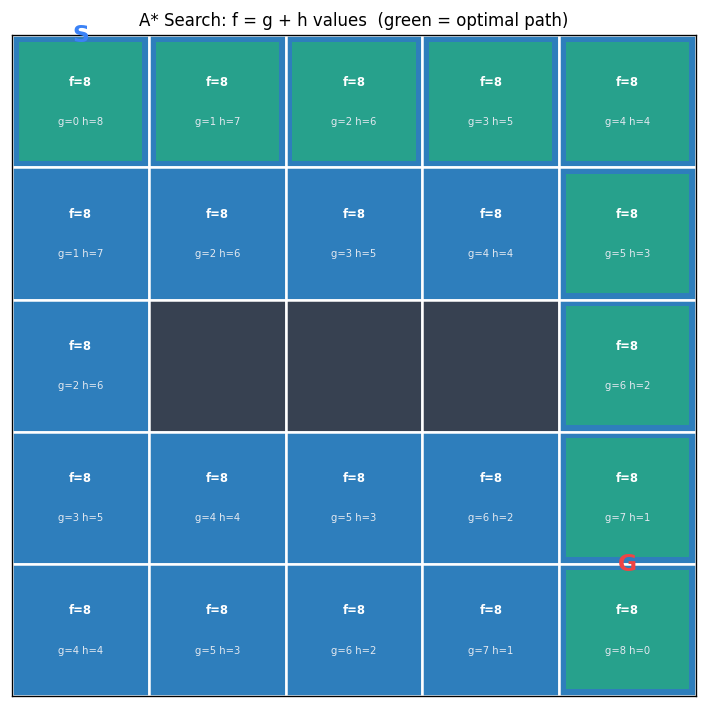
A* Search

The A* search algorithm is going to do much better than the greedy search algorithm because it takes advantage of the cost information as well. A* search implements the frontier as a priority queue, ordered by \(f(n)\) where \(n\) is the current node:

\[f(n) = cost(n) + h(n)\]

Think of \(f(n)\) as an estimate of the cost of the cheapest path from the start state to a goal state through the current state \(n\). Intuitively, A* combines the ideas of lowest-cost-first search and greedy best-first search.

Properties of A* Search

For complexity, A* does not do better than the other heuristic search algorithms — space and time complexity are both exponential. The heuristic function does not improve theoretical guarantees since the guarantees only consider the worst case. In practice, A* performs much better if the heuristic value is accurate.

A* is complete and optimal as long as the heuristic function satisfies a mild condition: the heuristic function must be admissible.

An admissible heuristic is one that does not over-estimate the cost of the cheapest path from the current node \(n\) to a goal node. Let \(h^*(n)\) be the cost of the cheapest path from \(n\) to a goal. Then we must have:

\[0 \leq h(n) \leq h^*(n)\]

You can think of an admissible heuristic as a lower bound on the actual cost of the best path, or like an optimistic person who always tells you a cost value that is smaller than the actual cost.

Furthermore, A* is optimally efficient: given a particular admissible heuristic \(h\), no search algorithm could do better. Among all the optimal algorithms that start from the same start node and use the same heuristic \(h\), A* expands the minimum number of paths \(p\) for which \(f(p) \neq f^*\), where \(f^*\) is the cost of the cheapest path.

Designing an Admissible Heuristic

Since A* has the nice property that if the heuristic function is admissible then it is guaranteed to find an optimal solution, an important question is: how do we come up with an admissible heuristic function?

Two Heuristics for the 8-Puzzle

Manhattan distance heuristic: For every tile on the puzzle except the empty one, compute the Manhattan distance (horizontal distance plus vertical distance) from its current position to its goal position, and sum all these distances. For the initial state with tiles 5,3,_,8,7,6,2,4,1, the Manhattan distance heuristic value is 16.

Misplaced tile heuristic: Count the number of non-empty tiles that are not in their goal positions. For the same initial state, seven out of the eight numbers are not in their goal positions, so the heuristic value is 7.

A Procedure for Constructing an Admissible Heuristic

The general procedure is:

1. Take the original problem and relax it. Usually the problem has some requirements expressed as constraints. Simplify the constraints or remove some constraints.
2. Solve the relaxed problem optimally. The cost of the optimal solution to the relaxed problem is an admissible heuristic function for the original problem.

It is important that the relaxed problem is easy to solve — solving it should not require search.

Constructing Admissible Heuristics for the 8-Puzzle

In the 8-puzzle, there are two requirements when moving a tile from position A to position B:

• A and B must be adjacent
• The target position B must be empty

Relaxation 1: Remove the “B must be empty” constraint (keep adjacency). A tile can move from square A to square B if A and B are adjacent. The optimal solution to this relaxed problem gives us the Manhattan distance heuristic.

Relaxation 2: Remove both constraints. A tile can move from any square A to any square B. Since we can move a tile directly to its goal position in one move, the optimal cost is just the number of misplaced tiles — this gives us the Misplaced tile heuristic.

A third heuristic can be derived by removing only the adjacency constraint (keeping “B must be empty”), which leads to Gaschnig’s heuristic (Gaschnig, 1979).

Comparing Heuristic Functions

When we have multiple admissible heuristic functions, which one should we choose?

First, we must require that the heuristic is admissible, so that A* can find the optimal solution. Next, it is nice if the heuristic function produces different values for different states — this helps us distinguish different states and decide which state to expand next. If the heuristic function is constant, it has the same value for all states, which is not very useful. Finally, we want the heuristic values to be as close to the true costs as possible — the more accurate the heuristic, the better.

Dominating Heuristic

Given heuristics \(h_1(n)\) and \(h_2(n)\), we say that \(h_2(n)\) dominates \(h_1(n)\) if and only if:

• \(\forall n: h_2(n) \geq h_1(n)\) (for every state, \(h_2\) produces a weakly higher value than \(h_1\)
• \(\exists n: h_2(n) > h_1(n)\) (there exists at least one state where \(h_2\) has a strictly larger value than \(h_1\)

One consequence of this relationship is that if \(h_2\) dominates \(h_1\), then running A* with \(h_2\) will not expand more nodes than running A* with \(h_1\). By using \(h_2\), A* will spend less time exploring the search graph and find an optimal solution faster.

For the 8-puzzle, the Manhattan distance heuristic dominates the misplaced tile heuristic. For every tile that is not in its goal position, the misplaced tile heuristic adds 1, while the Manhattan distance heuristic adds at least 1 (more if the positions are not adjacent). The Manhattan distance is always greater than or equal to the misplaced tile count, and strictly greater for many states.

Pruning the Search Space

It is often a good idea to combine search algorithms with pruning strategies. For example, depth-first search will not terminate on a graph with cycles, which can be solved with cycle pruning. For breadth-first search, using multiple-path pruning can reduce the number of nodes we need to expand and make the search more efficient.

Cycle Pruning

A cycle cannot be part of an optimal solution. As soon as we detect that we are in a cycle, we should discard the path right away. Cycles can cause problems for search algorithms — DFS gets trapped in the cycle and does not terminate.

To check whether the new node is in a cycle, we check whether it is on the current path. In the worst case, we need to go through all the nodes on the path — this takes time linear in the length of the path. However, for DFS, which only remembers one path at a time, we can store all nodes in a set or hash map and check in constant time.

procedure SEARCH(Graph, Start node s, Goal test goal(n))
  frontier := {⟨s⟩}
  while frontier is not empty do
    select and remove path ⟨n₀, ..., nₖ⟩ from frontier
    if goal(nₖ) then
      return ⟨n₀, ..., nₖ⟩
    for every neighbour n of nₖ do
      if n ∉ ⟨n₀, ..., nₖ⟩ then       // cycle check
        add ⟨n₀, ..., nₖ, n⟩ to frontier
  return no solution

Multiple-Path Pruning

When solving a search problem, we only need to find one path to any node. Once we have found a path to a node, we can discard all other paths to the same node. We maintain an explored set that stores all the nodes to which we have found a path. When we remove a path from the frontier, we check whether the last node is in the explored set. If it is, we discard the path. Otherwise, we expand the path and add the node to the explored set.

Cycle pruning is a special case of multi-path pruning — multi-path pruning subsumes cycle pruning.

procedure SEARCH(Graph, Start node s, Goal test goal(n))
  frontier := {⟨s⟩}
  explored := {}
  while frontier is not empty do
    select and remove path ⟨n₀, ..., nₖ⟩ from frontier
    if nₖ ∉ explored then
      add nₖ to explored
      if goal(nₖ) then
        return ⟨n₀, ..., nₖ⟩
      for every neighbour n of nₖ do
        add ⟨n₀, ..., nₖ, n⟩ to frontier
  return no solution

A Problem with Multi-Path Pruning

Multi-path pruning specifies that we should only keep the first path found to any node. But what if the first path is not the shortest path? For LCFS, multi-path pruning will not discard the optimal solution, because LCFS always explores paths in order of increasing costs — it will never find a longer path first and then a shorter path later.

For A* with an admissible heuristic, multi-path pruning can discard the optimal solution. The issue arises when the heuristic values cause A* to find a longer path to a node before a shorter path. The culprit is that admissibility allows the heuristic to overestimate the difference between the costs to reach intermediate nodes, even though it does not overestimate the total cost to the goal.

To fix this, we need a stronger condition on the heuristic. An admissible heuristic requires:

\[h(m) - h(g) \leq cost(m, g)\]

for any node \(m\) and any goal node \(g\). For A* with multi-path pruning to be optimal, the heuristic must satisfy a stronger condition for any node \(m\) and any other node \(n\):

\[h(m) - h(n) \leq cost(m, n)\]

If the heuristic satisfies this inequality, it is said to be a consistent heuristic. If the heuristic is consistent, then A* search with multi-path pruning is optimal.

Fortunately, most admissible heuristic functions are consistent. For example, in a multi-dimensional space, the Euclidean distance is often a consistent heuristic. It is challenging to come up with a heuristic that is admissible but not consistent. Therefore, it is often sufficient to construct an admissible heuristic and verify that it is also consistent using the definition.

Constraint Satisfaction Problems

Motivation for CSPs

In the previous lectures, the search algorithms we studied treated each state as a black box — the algorithms did not know or use the internal structure of states. This was a deliberate design choice, allowing us to use the same algorithm on many different problems. However, not knowing a state’s internal structure means the algorithm cannot detect that a partial state will never lead to a solution.

Consider the 4-queens problem. A partial state with only 2 queens might already violate the row constraint, making it impossible to reach a goal state. Knowing this internal structure allows us to prune large parts of the search tree. When we realize a partial state can never lead to a goal, we immediately backtrack and try something else.

A constraint satisfaction problem (CSP) explicitly models the internal structure of each state. These internal structures enable the development of specialized algorithms that solve CSPs much more efficiently than generic search.

Defining a CSP

A CSP is a special type of search problem. In addition to the usual components (initial state, goal test, successor function, cost function), we explicitly model the internal structure of a state with three components:

• A set \(X\) of variables: \(\{X_1, X_2, \ldots, X_n\}\)
• A set \(D\) of domains: \(D_i\) is the domain for variable \(X_i\)
• A set \(C\) of constraints specifying allowable value combinations

A solution to a CSP is an assignment of values to all the variables that satisfies all the constraints.

The 4-Queens Problem as a CSP

To formulate the 4-queens problem as a CSP, we assume there is exactly one queen per column. We define four variables \(x_0, x_1, x_2, x_3\), where the subscript \(i\) refers to the column and the value is the row position of the queen. The domain of each variable contains all four possible row positions: \(D_i = \{0, 1, 2, 3\}\) for each \(x_i\).

The constraints require that no two queens can be in the same row or the same diagonal, expressed mathematically as:

\[\forall_i \forall_j \; (i \neq j) \rightarrow ((x_i \neq x_j) \land (|x_i - x_j| \neq |i - j|))\]

The first part encodes the row constraint (different row positions), and the second part encodes the diagonal constraint (the difference in row positions cannot equal the difference in column positions).

Backtracking Search

CSPs can be solved using backtracking search, a special type of depth-first search. We use an incremental formulation: start with an empty board and add queens one by one from left to right, ensuring constraints are satisfied at each step.

The search components are:

• State: one queen per column in the leftmost \(k\) columns with no pair of queens attacking each other
• Initial state: no queens on the board
• Goal state: 4 queens on the board with no pair attacking each other
• Successor function: add a queen to the leftmost empty column such that it is not attacked by any existing queen

When tracing the backtracking algorithm on the 4-queens problem, we expand nodes in lexicographical order. Starting with the empty state, we place the first queen in row 0. After eliminating attacked positions, we find the second queen can only go in row 2 or 3. Choosing row 2 leads to a dead end (no valid position for the third queen), so we backtrack and try row 3. Continuing this process, we eventually find the solution state 1,3,0,2 — queens placed in rows 1, 3, 0, and 2 for columns 0 through 3 respectively.

The key advantage of backtracking search over plain DFS is that it recognizes when a partial state cannot possibly lead to a solution, immediately backtracking and pruning large portions of the search tree.

Arc Consistency

Motivation for Arc Consistency

When solving the 4-queens problem with backtracking search, placing the first queen in row 0 leads to a dead end — the entire leftmost subtree fails. Can we detect this dead end earlier without exploring it?

The answer is yes. Arc consistency helps us achieve this. After placing the first queen in row 0, we can eliminate positions for other queens by applying the row and diagonal constraints. Eventually, we discover that no valid positions remain for some variable, proving that the assignment \(x_0 = 0\) cannot lead to a solution.

Constraint Graphs

To apply arc consistency, we represent a CSP as a constraint graph. Nodes represent variables, and undirected arcs represent constraints. For the 4-queens problem, we have four nodes and six constraints (one between every pair of variables). If there are multiple constraints between two variables, we combine them into one.

The number of variables involved in a constraint is called its arity. A unary constraint involves one variable, a binary constraint involves two. Any constraint of higher arity can be decomposed into binary constraints by introducing additional variables, so it suffices to consider only binary constraints in a constraint graph.

Definition of Arc Consistency

Given two variables \(X\) and \(Y\) with domains \(D_X\) and \(D_Y\), joined by a constraint \(c(X,Y)\), each binary constraint has two arcs: \(\langle X, c(X,Y) \rangle\) and \(\langle Y, c(X,Y) \rangle\). The first element of the tuple is the primary variable.

The arc \(\langle X, c(X,Y) \rangle\) is arc-consistent if and only if for every value \(v\) in \(D_X\), there exists a value \(w\) in \(D_Y\) such that \((v, w)\) satisfies the constraint \(c(X,Y)\). In predicate logic:

\[\langle X, c(X,Y) \rangle \text{ is arc-consistent} \iff \forall v \in D_X \; \exists w \in D_Y \; (v,w) \text{ satisfies } c(X,Y)\]

An important property: arc consistency is not symmetric. If \(\langle X, c(X,Y) \rangle\) is arc-consistent, it does not necessarily mean that \(\langle Y, c(X,Y) \rangle\) is also arc-consistent. Both arcs must be verified separately.

If an arc is not consistent, we can remove values from the primary variable’s domain to make it consistent. This domain reduction never eliminates valid solutions — it only removes values that cannot participate in any solution.

The AC-3 Algorithm

The AC-3 algorithm, proposed by Alan Mackworth in 1977, uses arc consistency to reduce variable domains and bring us closer to solving a CSP. The algorithm works as follows:

procedure AC-3
  S := every arc in the constraint graph
  while S is not empty do
    select and remove ⟨X, c(X,Y)⟩ from S
    remove every value in D_X that doesn't have a
      supporting value in D_Y satisfying c(X,Y)
    if D_X was reduced then
      if D_X is empty then return false
      for every Z ≠ Y, add ⟨Z, c'(Z,X)⟩ to S
  return true

The algorithm initializes a set S with every arc. It repeatedly selects and removes an arc, makes it arc-consistent by removing unsupported values from the primary variable’s domain, and if the domain was reduced, adds back arcs where the reduced variable is the secondary variable (except for the arc to Y, since reducing X’s domain cannot break arc consistency from Y’s perspective).

Why Add Arcs Back?

The most confusing part of AC-3 is why we add arcs back to S after reducing a domain. Consider an arc \(\langle X, c(X,Y) \rangle\) that was previously verified as arc-consistent. If we later remove a value from \(D_Y\), the arc \(\langle X, c(X,Y) \rangle\) may no longer be arc-consistent — the support for some value in \(D_X\) might have been the removed value in \(D_Y\). In contrast, reducing the primary variable’s domain (\(D_X\) cannot break the arc’s consistency, since fewer values need support.

Tracing AC-3 on the 4-Queens Problem

Starting with \(x_0 = 0\) and full domains for the other variables, AC-3 systematically reduces domains:

1. Processing \(\langle x_1, c(x_0, x_1) \rangle\): removes 0 and 1 from \(D_{x_1}\), leaving \(\{2, 3\}\)
2. Processing \(\langle x_2, c(x_0, x_2) \rangle\): removes 0 and 2, leaving \(\{1, 3\}\)
3. Processing \(\langle x_3, c(x_0, x_3) \rangle\): removes 0 and 3, leaving \(\{1, 2\}\)
4. Further propagation reduces \(x_2\) to \(\{3\}\), then \(x_3\) to \(\{1\}\)
5. Eventually \(x_2\)’s domain becomes empty — AC-3 returns false

This confirms that \(x_0 = 0\) has no solution, matching our earlier finding with backtracking search, but detected without any search.

Properties of AC-3

Does arc processing order matter? No — any order leads to the same final domains.

Three possible outcomes:

1. A domain becomes empty → no solution exists
2. Every domain has exactly one value → unique solution found
3. Every domain has at least one value and at least one has multiple → AC-3 is inconclusive; search or domain splitting is needed

Termination: AC-3 is guaranteed to terminate.

Complexity: With \(n\) variables, at most \(d\) values per domain, and \(c\) binary constraints, there are \(2c\) arcs. Each arc can be re-added at most \(d\) times, and checking consistency takes \(O(d^2)\). The overall runtime is \(O(cd^3)\).

Local Search

Introduction

The search algorithms discussed so far explore the search space systematically, which can be very slow if the space is too large or infinite. They also track paths from the initial state to the goal, which is unnecessary for many problems. For the 4-queens problem, the order in which queens are placed does not matter — only the final board matters.

Local search addresses both concerns by giving up on systematic exploration and path tracking. Local search algorithms explore only a portion of the search space in an ad hoc way, requiring very little memory. They can find solutions quickly on average and work well for CSPs and general optimization problems. However, they provide no guarantee that a solution will be found even if one exists.

What Is Local Search?

Local search starts with a complete assignment of values to all variables and iteratively improves the solution. This contrasts with the incremental formulation used for backtracking search, where we started with an empty state and built it step by step.

Components of a Local Search Problem

A local search problem consists of:

• A state: a complete assignment to all variables
• A neighbour relation: which states to explore next
• A cost function: how good each state is

For the 4-queens problem formulated as local search, the variables are \(x_0, x_1, x_2, x_3\) (row positions), the initial state has 4 queens in random positions, the goal is zero attacking pairs, and the cost function counts the number of pairs of queens attacking each other. Two natural neighbour relations are: (A) move a single queen to a different row in the same column, or (B) swap the row positions of two queens.

Iterative Best Improvement (Greedy Descent)

The first local search algorithm is greedy descent (also called hill climbing when maximizing a fitness function). The algorithm starts with a random state, moves to the neighbour with the lowest cost if it improves the current state, and stops when no neighbour has a lower cost.

Greedy descent can be summarized as: descend into a canyon in a thick fog with amnesia. Descending means minimizing cost. The thick fog means only seeing immediate neighbours. Amnesia means no memory of where we have been.

Properties of Greedy Descent

Greedy descent performs well in practice, often making rapid progress toward a solution. However, it is not guaranteed to find the global optimum given enough time — it can get stuck at local optima.

A local optimum is a state where no neighbour has a strictly lower cost. A global optimum is a state with the lowest cost among all states — it is a special case of a local optimum.

There are several types of problematic regions in the search landscape: strict local optima (valleys that are not the deepest), flat local optima (plateaus where all neighbours have equal cost), and shoulders (flat regions that eventually lead downhill).

Escaping Flat Local Optima

To escape flat local optima, we can allow sideway moves: the algorithm moves to a neighbour with the same cost. To ensure termination, we limit the number of consecutive sideway moves. A tabu list — a short-term memory of recently visited states — prevents cycling.

For the 8-queens problem (approximately 17 million states), greedy descent without sideway moves solves only 14% of instances in 3-4 steps. With up to 100 consecutive sideway moves allowed, the success rate jumps to 94%, though at the cost of more steps (21 on success, 64 on failure).

Greedy Descent with Randomization

Two randomization strategies help escape even strict local optima:

Random restarts: Jump to an entirely different part of the search space and run greedy descent again. This is effective for smooth landscapes with few, wide local optima — random walks would not escape the large valleys.

Random walks: Occasionally move to a higher-cost neighbour. This is effective for jagged landscapes with many small local optima — random restarts would just land in another local optimum.

Greedy descent with random restarts runs greedy descent multiple times from random initial states and keeps the best result. Given enough time, this approach finds the global optimum with probability approaching 1, since eventually the random start will be the global optimum itself.

Simulated Annealing

Simulated annealing combines optimization (exploitation) with exploration. Inspired by the physical process of slowly cooling molten metals, the algorithm starts with a high temperature and reduces it slowly.

At each step, the algorithm chooses a random neighbour. If the neighbour is an improvement, it moves there. If not, it moves with probability \(p = e^{-\Delta C / T}\), where \(\Delta C = \text{cost}(A') - \text{cost}(A) > 0\) is the cost increase and \(T\) is the current temperature.

Two key properties of this probability function:

• As \(T\) decreases, we are less likely to move to a worse neighbour (more conservative over time)
• As \(\Delta C\) increases, we are less likely to move to the neighbour (worse neighbours are riskier)

procedure SIMULATED-ANNEALING
  current ← initial-state
  T ← a large positive value
  while T > 0 do
    next ← a random neighbour of current
    ΔC ← cost(next) - cost(current)
    if ΔC < 0 then
      current ← next
    else
      current ← next with probability p = e^(-ΔC/T)
    decrease T
  return current

The annealing schedule determines how \(T\) decreases. A popular choice is geometric cooling: multiply \(T\) by a factor close to 1 (e.g., 0.99) at each step. Starting with \(T = 10\) and multiplying by 0.99, after 500 steps \(T \approx 0.07\). If the temperature decreases slowly enough, simulated annealing is guaranteed to find the global optimum with probability approaching 1.

An analogy: imagine a hilly surface where we drop a tennis ball and want it to reach the deepest valley. Gravity pulls the ball down (optimization), but we shake the surface to bounce the ball around (exploration). Initially we shake vigorously; over time we shake less, and the ball settles into a deep valley.

Population-Based Algorithms

All local search algorithms so far maintain a single state. Population-based algorithms maintain multiple states simultaneously, allowing information sharing between parallel searches.

Beam Search

Beam search maintains \(k\) states. At each step, it generates all neighbours of the entire population and keeps the \(k\) best. When \(k = 1\), beam search reduces to greedy descent. Unlike \(k\) random restarts in parallel (where searches are independent), beam search shares information — a state in a promising region contributes many neighbours to the next population. However, beam search suffers from lack of diversity: the population can quickly concentrate in a small region.

Stochastic Beam Search

Stochastic beam search addresses the diversity problem by choosing the next \(k\) states probabilistically rather than deterministically. The probability of choosing a neighbour is proportional to its fitness. This mimics natural selection — neighbours are like offspring, and survival depends on fitness. Stochastic beam search is analogous to asexual reproduction.

Genetic Algorithm

The genetic algorithm extends the biological analogy to sexual reproduction. It maintains a population of \(k\) states and probabilistically selects two parent states (with probability proportional to fitness) to produce a child through crossover — combining portions of each parent. The child may also undergo mutation (random small changes). This process repeats until a stopping criterion is met.

Introduction to Machine Learning

Introduction to Learning

Machine learning has been hugely successful in many applications: medical diagnosis (processing MRI, X-ray, and CT images), facial recognition, handwriting recognition, speech recognition, and spam filtering.

Learning is the ability of an agent to improve its performance on future tasks based on experience. We want agents that can do more, do things better, and do things faster. Learning is essential because we cannot anticipate all possible solutions, all changes over time, and for some tasks we may not know how to program a solution directly.

The Learning Architecture

Any learning problem has four key components:

• Problem/task: the behaviour we want to improve
• Experiences/data: the training examples
• Background knowledge/bias: initial knowledge that may bias performance
• Measure of improvement: how we track progress

Types of Learning Problems

Learning problems fall into three broad categories:

Supervised learning: Given input features, target features, and training examples, predict target features for new examples. This requires labeled data — each training example has a known correct answer.

Unsupervised learning: Learning from examples without target labels. Examples include clustering (grouping similar examples) and dimensionality reduction (projecting high-dimensional data to lower dimensions).

Reinforcement learning: Learning from rewards and punishments, somewhere between supervised (exact feedback) and unsupervised (no feedback).

Classification vs. Regression

Supervised learning problems divide into two categories:

• Classification: target features are discrete (e.g., classifying weather as sunny, cloudy, or rainy)
• Regression: target features are continuous (e.g., predicting tomorrow’s temperature)

Supervised Learning

In supervised learning, we are given training examples of the form \((x, f(x))\), where \(x\) is a vector of input features and \(f(x)\) is the target. We return a hypothesis \(h\) that approximates the true function \(f\).

Learning as a Search Problem

Learning can be viewed as searching through a hypothesis space. We need:

• A search space of hypotheses
• An evaluation function to compare hypotheses
• A search method to explore the space

Often the hypothesis space is prohibitively large for systematic search, so machine learning techniques use local search methods.

Generalization

The goal of machine learning is not to find a function that fits all training examples perfectly, but to find a hypothesis that can predict unseen examples correctly. A hypothesis that predicts unseen examples well is said to generalize well.

Two techniques for choosing a hypothesis that generalizes:

• Ockham’s razor: prefer the simplest hypothesis consistent with the data
• Cross-validation: a more principled approach to estimating generalization error

Bias-Variance Trade-off

The bias-variance trade-off explains how model performance changes with complexity:

• Bias describes how well we can fit the data with infinite training data. High bias means the model is too simplistic — strong assumptions, few degrees of freedom, poor fit to training data.
• Variance describes how much the learned hypothesis varies given different training data. High variance means the model is too flexible — changes drastically with the data, fits training data well but generalizes poorly (over-fitting).

The optimal model complexity balances these two sources of error. Too simple → high bias (under-fitting). Too complex → high variance (over-fitting). The sweet spot is in the middle.

Cross-Validation

Cross-validation is a principled technique for finding a model with low bias and low variance. The steps are:

1. Break the training data into \(K\) equally sized partitions
2. Train on \(K-1\) partitions (training set)
3. Test on the remaining partition (validation set)
4. Repeat \(K\) times, each time using a different partition for validation
5. Calculate the average error over the \(K\) validation sets

This gives a reliable estimate of how well the model generalizes.

Over-Fitting

As model complexity increases, the error on the training set always decreases. However, the validation set error follows a U-shape: it first decreases (under-fit region), reaches a minimum (best fit), then increases (over-fit region). The best model has enough complexity to capture the common patterns but not so much that it over-fits to training-specific characteristics.

Decision Trees

Examples of Decision Trees

Our first machine learning algorithm is the decision tree. A decision tree is a very common algorithm that we humans use daily — “Which language should you learn?”, “What kind of pet is right for you?”, and “Should you use emoji?” are all examples of decision tree reasoning.

We will use the following running example throughout this unit: Jeeves is a valet to Bertie Wooster. Each morning, Jeeves records the weather (Outlook, Temperature, Humidity, Wind) and whether Bertie plays tennis. The training set has 14 examples.

Definition and Classification

A decision tree is a simple model for supervised classification. Each internal node performs a test on an input feature. The edges are labeled with the feature values. Each leaf node specifies a value for the target feature. If we convert a decision tree to a program, it becomes a big nested if-then-else structure.

To classify an example, we traverse down the tree, evaluating each test and following the corresponding edge until we reach a leaf. The classification on that leaf is our prediction.

The Decision Tree Learning Algorithm

Issues in Learning a Decision Tree

Given a data set, we can generate many different decision trees. Two key decisions must be made:

1. What order to test features? Different orders produce different trees. Finding the optimal order is computationally expensive, so we use a greedy (myopic) approach — choosing the best feature at each step without considering future effects.
2. Should we grow a full tree or stop early? A full tree may over-fit the training data, so a smaller tree might generalize better (Occam’s razor).

Growing a Full Tree

To build a tree given a testing order: at each node, check if all examples share the same class. If so, create a leaf with that class label. Otherwise, test the next feature and split examples into branches. Repeat recursively.

Stopping Criteria

There are three base cases:

1. All examples are in the same class → return the class label
2. No features left (noisy data) → return the majority class
3. No examples left (unseen feature combination) → use the parent node’s examples and return the majority class

Pseudocode

procedure DECISION-TREE-LEARNER(examples, features)
  if all examples are in the same class then
    return the class label
  else if no features left then
    return the majority decision
  else if no examples left then
    return the majority decision at the parent node
  else
    choose a feature f
    for each value v of feature f do
      build edge with label v
      build sub-tree using examples where f = v

Determining the Order of Testing Features

We want to choose the feature that makes the biggest difference to the classification — the feature that reduces our uncertainty the most. This is measured by the expected information gain.

Entropy

Entropy from information theory measures the uncertainty in a probability distribution. For a distribution over \(k\) outcomes with probabilities \(P(c_1), \ldots, P(c_k)\):

\[I(P(c_1), \ldots, P(c_k)) = -\sum_{i=1}^{k} P(c_i) \log_2(P(c_i))\]

For a binary distribution \((p, 1-p)\): entropy is maximized at 1 bit when \(p = 0.5\) (uniform distribution, maximum uncertainty) and minimized at 0 bits when \(p = 0\) or \(p = 1\) (point mass, no uncertainty). By convention, \(0 \cdot \log_2(0) = 0\).

Expected Information Gain

Consider a feature with \(k\) values \(v_1\) to \(v_k\). Before testing, we have \(p\) positive and \(n\) negative examples. The entropy before testing is:

\[I_{\text{before}} = I\left(\frac{p}{p+n}, \frac{n}{p+n}\right)\]

After testing, the expected entropy is the weighted average of the entropy of each branch:

\[EI_{\text{after}} = \sum_{i=1}^{k} \frac{p_i + n_i}{p + n} \cdot I\left(\frac{p_i}{p_i + n_i}, \frac{n_i}{p_i + n_i}\right)\]

The expected information gain is the difference:

\[\text{InfoGain} = I_{\text{before}} - EI_{\text{after}}\]

We select the feature with the highest expected information gain. This greedy algorithm for building a decision tree by selecting the most informative feature at each step is known as ID3.

A Full Example

For the Jeeves dataset (9 positive, 5 negative), the entropy before any split is approximately 0.94 bits. Computing information gain for each feature:

Feature	Gain
Outlook	0.247
Humidity	0.151
Wind	0.048
Temp	0.029

Outlook has the highest gain, so it becomes the root. For the Overcast branch, all examples are positive (entropy 0, pure node). For Sunny and Rain, we continue splitting. In the Sunny branch, Humidity has the highest gain (0.97); in the Rain branch, Wind has the highest gain (0.97). The resulting tree is small and shallow — exactly what we wanted.

Real-Valued Features

So far, the algorithm handles only discrete features. For real-valued features (like temperature as a number rather than Hot/Mild/Cool), we use binary splits.

Choosing a Split Point

To handle a real-valued feature:

1. Sort the instances by the feature value
2. Identify possible split points at midpoints between consecutive values where the target label changes
3. Calculate the expected information gain for each split point
4. Choose the split point with the highest gain

A midpoint \((X + Y)/2\) between consecutive values \(X\) and \(Y\) is a possible split point only if the labels at \(X\) and \(Y\) differ. This smart approach reduces the number of candidate split points from \(n-1\) to only those where the label actually changes.

Over-Fitting

Decision trees are simple, interpretable, and work well even with tiny datasets. However, over-fitting is a common problem. The decision tree learner is a perfectionist — it keeps growing until it perfectly classifies all training examples, which can be undesirable.

Consider the Jeeves dataset with one corrupted data point (day 3 changed from Yes to No). This tiny change causes the algorithm to grow an entire subtree for the Overcast branch (which was previously a pure Yes leaf), dramatically changing the tree and increasing the test error from 0/14 to 2/14.

Dealing with Over-Fitting: Pruning

Two approaches to prevent over-fitting:

Pre-pruning (stop growing the tree early): We use criteria to decide when to stop splitting:

1. Maximum depth: stop if the tree reaches a preset depth
2. Minimum examples: stop if too few examples remain at a node
3. Minimum information gain: stop if the gain from splitting is too small
4. Reduction in training error: stop if the error reduction is below a threshold

Post-pruning (grow a full tree, then trim): Post-pruning is particularly useful when individual features are uninformative but multiple features working together are very informative (as in the XOR problem). With pre-pruning, we would stop too early because each feature alone has zero information gain. With post-pruning, the full tree is grown first, capturing the joint effect, and then trimmed where subtrees do not help. To post-prune, we examine nodes whose children are all leaves: if the information gain is below a threshold, we replace the subtree with a single leaf using the majority class.

Neural Networks, Part 1

Introduction to Artificial Neural Networks

There is currently a great deal of excitement around neural networks. To understand why, it helps to situate them within the broader landscape of artificial intelligence. Artificial intelligence is the endeavour of building machines that behave intelligently. Machine learning is a branch of AI that lets computers learn without being explicitly programmed, primarily using statistical methods. Deep learning is a branch of machine learning that develops hierarchical networks that mimic the human brain.

Deep learning has been around for decades, but it only became very successful in the late 2000s. Two factors drove this resurgence: the availability of more powerful computers and access to vast amounts of data.

Two landmark events from 2012 illustrate this success. First, a deep learning algorithm called AlexNet won the ImageNet challenge, a supervised learning application in image classification. Second, the Google Brain project made a breakthrough in unsupervised learning: after processing over 10 million images from YouTube videos, one node of the neural network developed a strong affinity for cats and was able to recognize when an image contained a cat. This has been called the infamous Cat Experiment.

Learning Complex Relationships

Consider applications such as image interpretation, speech recognition, or machine translation. In all of these, the relationship between inputs and outputs is complex. How can we build a model to learn such complex relationships? Humans can learn these relationships very well, so the original motivation for artificial neural networks was to build a model that mimics the human brain.

The Human Brain

Thanks to neuroscience, we have some understanding of the structure of the human brain. The brain is a set of densely connected neurons. Each neuron is a very simple unit with several key components: dendrites receive inputs from other neurons, the soma controls the activity of the neuron, the axon sends outputs to other neurons, and synapses link neurons together. A neuron takes input, does some simple computation, and decides on the strength of its output.

As a computational model, this contrasts with other models we have encountered. For example, a random forest combines multiple decision trees, and each model is very complex. The model of the human brain is very different: it has a large number of simple components rather than a small number of complex components. No one model is inherently better than another.

A Simple Mathematical Model of a Neuron

McCulloch and Pitts first proposed this model of a neuron in 1943. It is a very simple model; actual neurons have much more complex behaviour. The model says that a neuron is a linear classifier: it “fires” when a linear combination of its inputs exceeds some threshold.

Neuron \( j \) computes a weighted sum of its input signals \( a_i \), where \( w_{ij} \) is a weight on the connection from unit \( i \) to unit \( j \):

\[ in_j = \sum_{i=0}^{n} w_{ij} a_i \]

Neuron \( j \) then applies an activation function \( g \) to the weighted sum to derive the output:

\[ a_j = g(in_j) = g\left( \sum_{i=0}^{n} w_{ij} a_i \right) \]

Notice that the input \( a_0 \) is always set to 1; this is called a bias or dummy input. Because our model is a linear classifier, we want to represent a linear function, but our inputs are all variables. We need the possibility of having a constant term. Setting \( a_0 = 1 \) lets us have that constant term through the weight \( w_{0j} \).

Desirable Properties of the Activation Function

The activation function is very important in our model. There are three desirable properties an activation function should have.

First, it should be non-linear. Combining linear functions will not produce a non-linear function, but complex relationships are often non-linear. Using a non-linear activation function allows us to model non-linear relationships by interleaving linear functions (weighted sums of inputs) with non-linear functions (activation functions).

Second, it should mimic the behaviour of real neurons. If the weighted sum of input signals is large enough, the neuron fires. Otherwise, it does not fire. There is no need for a hard threshold; the function can fire an output signal of some amount.

Third, it should be differentiable almost everywhere. We want to learn a neural network using gradient descent or other optimization algorithms, which require the activation function to be differentiable.

Common Activation Functions

The step function is defined as:

\[ g(x) = \begin{cases} 1 & \text{if } x > 0 \\ 0 & \text{if } x \le 0 \end{cases} \]

It is simple to use but not differentiable, so it is not used in practice. It is useful for explaining concepts.

The sigmoid function is defined as:

\[ g(x) = \frac{1}{1 + e^{-kx}} \]

The sigmoid can approximate the step function (larger \( k \) gives a better approximation). It gives clear, bounded predictions and is differentiable. It was preferred for a long time but suffers from the vanishing gradient problem: the gradient is very small for extreme values of \( x \), and it is computationally expensive.

The rectified linear unit (ReLU) is defined as:

\[ g(x) = \max(0, x) \]

It is computationally efficient, non-linear, and differentiable. However, it suffers from the dying ReLU problem: the gradient is 0 for negative \( x \) or \( x \) approaching 0, which can prevent learning.

The leaky ReLU is defined as:

\[ g(x) = \max(0.1x, x) \]

It behaves like a ReLU but enables learning for negative input values by allowing a small, non-zero gradient when \( x < 0 \).

Introduction to Perceptrons

Feed-Forward vs. Recurrent Neural Networks

There are two major types of neural networks. A feed-forward neural network is a directed acyclic graph with no loops. Values flow in one direction through the network: they come in as input values, get transformed through the edges and nodes, and finally go out as output values. They never go backwards. In a feed-forward network, the outputs are a function of the inputs alone. If you know the inputs, you can determine the outputs.

A recurrent neural network can have loops. An output from a node can be fed back into the node as an input. The advantage of having a loop is that it gives the network memory: the circuit can remember some information while it is doing computations. The output value is no longer a function of its inputs alone; it may also depend on what the network remembers about the historical inputs. Arguably, a recurrent network is a better model of the human brain because we have memory. Unfortunately, because of the loops, it is also more difficult to train a recurrent network and to interpret its learned function. In this course we focus on feed-forward networks.

Perceptrons

A perceptron is a single-layer feed-forward neural network. It has two layers: the input layer and the output layer. However, the input layer does not have neurons; it simply contains the input values. The output layer has neurons, each of which takes the input values, calculates the weighted sum, and feeds the result through an activation function to produce the output.

A perceptron can represent simple logical functions such as AND, OR, and NOT. This was a big deal when it was discovered. At the time, much of AI focused on developing systems to perform formal logical reasoning. Representing logical functions was seen as the first step towards building a powerful logical deduction system.

Although a perceptron may appear to have two output neurons, if the two outputs are independent we can split the network into two independent perceptrons and learn the weights in each one separately. Thus we can focus on discussing a single perceptron at a time.

Determining the logical function of a perceptron. Consider a perceptron with two inputs \( x_1 \) and \( x_2 \), a bias weight of 0.5, and weights of \( -1 \) on both \( x_1 \) and \( x_2 \), using the step function as the activation function. To determine which logical function this computes, we draw a truth table:

\( x_1 \)	\( x_2 \)	\( o_1 \)
0	0	1
0	1	0
1	0	0
1	1	0

The output is 1 only when both inputs are 0, and 0 otherwise. This is a negation of the OR function: \( o_1 = \neg(x_1 \lor x_2) \).

Learning weights for the AND function. Consider a perceptron with unknown weights \( w_{01} \), \( w_{11} \), and \( w_{21} \) and the step function as activation. We want to find weights so that the perceptron represents the AND function. The key insight is that a perceptron is a linear classifier. Given the data points, we need to find a line that separates the positive examples from the negative examples. We can then derive an inequality that selects the side with the positive examples, and read off the weights from the coefficients.

For the AND function, we draw the inputs in the \( x_1 x_2 \)-plane and shade in the inputs that correspond to an output of 1 (only the point \( (1,1) \). A line with \( x_1 \) and \( x_2 \) intercepts of 1.5 and a slope of \( -1 \) works. The line is \( x_2 = -x_1 + 1.5 \), which we rewrite as \( x_1 + x_2 - 1.5 = 0 \). Since the point \( (1,1) \) should be on the positive side, we need \( x_1 + x_2 - 1.5 > 0 \), which is satisfied since \( 1 + 1 - 1.5 = 0.5 > 0 \). Reading off the coefficients: \( w_{01} = -1.5 \), \( w_{11} = 1 \), \( w_{21} = 1 \).

Limitations of Perceptrons

The First AI Winter

From the 1950s to the 1960s, research into perceptrons seemed very promising. People believed AI could be solved if computers could be made to perform formal logical reasoning, and perceptrons could represent simple logical functions like AND, OR, and NOT – the building blocks of a logical deduction system.

Unfortunately, in the late 1960s, limitations of perceptrons were discovered. Marvin Minsky, the founder of the MIT AI lab, and Seymour Papert, the director of the lab, studied perceptrons and found a significant limitation. They recorded their findings in a book called Perceptrons: An Introduction to Computational Geometry. In the book, Minsky and Papert showed that it is not possible to represent an XOR function using perceptrons alone – a deeper network with at least two layers is needed. The XOR of two inputs is true whenever the two inputs are different: they are either 1 and 0, or 0 and 1.

This fact by itself is not a problem. If a deeper network is needed, one could be constructed and trained. Unfortunately, at the time, nobody knew how to train a neural network with at least two layers. People only knew how to train a perceptron – a single-layer network. These two results combined suggested that pursuing perceptrons may be a dead end. This discovery had a huge impact on neural network research and led to the first AI winter: a freeze on funding for neural networks and great difficulty publishing papers on the topic.

Why can a perceptron not represent XOR? Intuitively, a perceptron with the step function as its activation function is a linear classifier, but XOR is not linearly separable. In a plot of the input space, AND and OR each have their positive examples on one side of a line, but for XOR no single line can separate the positive examples from the negative ones.

We can prove this rigorously. Assume towards a contradiction that we can represent XOR with a perceptron using the step function. The four input points give us four inequalities based on the required classification:

\[ w_{21} \cdot 1 + w_{11} \cdot 0 + w_{01} > 0 \quad (1) \]\[ w_{21} \cdot 0 + w_{11} \cdot 1 + w_{01} > 0 \quad (2) \]\[ w_{21} \cdot 1 + w_{11} \cdot 1 + w_{01} \le 0 \quad (3) \]\[ w_{21} \cdot 0 + w_{11} \cdot 0 + w_{01} \le 0 \quad (4) \]

From (1): \( w_{21} > -w_{01} \). From (2): \( w_{11} > -w_{01} \). Adding these gives \( w_{21} + w_{11} > -2w_{01} \). From (4): \( w_{01} \le 0 \), so \( -2w_{01} \ge -w_{01} \). From (3): \( w_{21} + w_{11} \le -w_{01} \). Combining: \( w_{21} + w_{11} > -2w_{01} \ge -w_{01} \ge w_{21} + w_{11} \), which is a contradiction. Therefore a perceptron cannot represent XOR.

XOR as a 2-Layer Neural Network

Since we cannot represent XOR with a single-layer network, how can we represent it? The simplest network that works has three layers: the input layer, a hidden layer, and the output layer. The input layer is not a real layer since it does not perform any computation. The middle layer is called a hidden layer because it is not visible, whereas the input and output are the two visible layers. In a larger network, any layer in the middle is a hidden layer.

To find the weights, we decompose XOR into simpler functions that perceptrons can represent. Recall that XOR can be expressed as:

\[ o_1 = (x_1 \lor x_2) \land (\neg(x_1 \land x_2)) \]

We can represent all of these simpler AND, OR, and NOT components with perceptrons. One solution uses two hidden units: \( h_1 \) computes \( x_1 \lor x_2 \) (OR), and \( h_2 \) computes \( \neg(x_1 \land x_2) \) (NAND). The output unit then computes \( h_1 \land h_2 \) (AND).

The specific weights are: from the input layer to \( h_1 \), the bias weight is \( -0.5 \) and the weights on \( x_1 \) and \( x_2 \) are both 1. For \( h_2 \), the bias weight is 1.5 and the weights on \( x_1 \) and \( x_2 \) are both \( -1 \). For the output unit, the bias weight is \( -1.5 \) and the weights on \( h_1 \) and \( h_2 \) are both 1. The formulas and truth tables verify the correctness:

\( h_1 = g(x_1 + x_2 - 0.5) \), which computes \( x_1 \lor x_2 \).

\( h_2 = g(-x_1 - x_2 + 1.5) \), which computes \( \neg(x_1 \land x_2) \).

\( o_1 = g(h_1 + h_2 - 1.5) \), which computes \( h_1 \land h_2 \).

Indeed, \( o_1 = (h_1 \land h_2) = ((x_1 \lor x_2) \land (\neg(x_1 \land x_2))) = x_1 \oplus x_2 \).

---

Neural Networks, Part 2

Gradient Descent

A Motivating Example

Throughout this lecture, we work with a simple two-layer feed-forward neural network. The input layer has three nodes (one of which is a dummy bias node with value 1), the hidden layer also has three nodes (one dummy), and the output layer has two nodes. Our goal is to learn the weights \( Wk_{ij} \) such that the actual outputs \( z2_1 \) and \( z2_2 \) are close to the expected values given by the training data.

Introduction to Gradient Descent

Gradient descent is a well-known optimization algorithm that can be thought of as a local search algorithm to find the minimum of a function. Consider a search space whose dimension is given by the number of weights in the neural network. We want to find a combination of weights that minimizes the total error made on the training examples. Gradient descent is very similar to greedy descent, but differs in that we are now dealing with continuous rather than discrete values. Accordingly, we use the gradient, or partial derivative, to determine the direction and size of each step we want to take. The function in this case is the error function: the difference between the expected outputs based on the training data and the actual outputs based on the network.

An intuitive way to understand gradient descent is the quotation: “Walking downhill and always taking a step in the direction that goes down the most.” We descend to the minimum by following the steepest direction at each step.

Steps of the Algorithm

The gradient descent algorithm proceeds as follows:

1. Initialize the weights randomly.
2. For each training example, change each weight in proportion to the negative of the partial derivative of the error with respect to that weight. Overall, update a weight \( w \) by:

\[ w := w - \sum_{\text{examples}} \eta \frac{\partial \text{error}}{\partial w} \]

Here, \( \eta \) is a constant called the learning rate.

3. Terminate after some number of steps when the error is small enough or when the changes to the weights become sufficiently small.

Deriving Intuition for Gradient Descent

Consider a simple function \( y = x^2 \). We want to minimize this function starting from some point \( x_0 \); the minimum is at \( x = 0 \).

If we start to the right of the minimum, the derivative \( \frac{dy}{dx} > 0 \), and to decrease our value we should move in the direction of the negative of the gradient (to the left). If we start to the left of the minimum, the derivative \( \frac{dy}{dx} < 0 \), and to increase our value we should again move in the direction of the negative of the gradient (to the right). In both cases, moving in the negative gradient direction brings us closer to the minimum.

As for magnitude, the gradient is zero at the minimum. In a region where the gradient is large in magnitude, we must be far from the minimum (assuming the function is continuous), so we can afford to take a larger step. In a region where the gradient is small in magnitude, we are likely close to the minimum and should take a smaller step to avoid overshooting.

Alternative Ways to Update the Weights

In the standard version of gradient descent, the weights are updated after sweeping through all training examples. But when the training data set is large, this means weight updates are very infrequent.

To speed up learning, we can update weights after each example. This variant is called incremental gradient descent. A related variant is stochastic gradient descent, where we randomly choose an example at each step instead of proceeding sequentially. The advantage of incremental gradient descent is increased learning speed since the weights are updated much more frequently. The disadvantage is that we may not converge to the local minimum – a single example may take us away from rather than towards it.

To balance these trade-offs, we have batched gradient descent, which updates the weights after a batch of examples. The batch size can be chosen along a spectrum: a batch size of one is identical to incremental gradient descent, and putting all examples into the batch is identical to standard gradient descent. A common strategy is to start with small batches to learn quickly, then gradually increase the batch size until the weights eventually converge.

The Back-Propagation Algorithm

Introducing the Back-Propagation Algorithm

The most challenging step in gradient descent is calculating the gradient for each weight. We could write down an expression for the gradient for each weight and calculate it directly, but this approach is quite inefficient. Modern neural networks tend to be very large, with thousands or more weights to learn. The back-propagation algorithm is an efficient way of calculating the gradients for all the weights.

Consider a setting where we have \( n \) training examples. For each training example, \( x \) consists of the input feature values and \( y \) is the label (expected output). To evaluate how close the actual output values \( z2 \) are to the expected output values \( y \), we use an error/loss function \( E \). When we execute gradient descent, our goal is to minimize the error \( E \) by adjusting the weights in the neural network.

Given the training examples, we calculate the gradients by performing two passes in the network: a forward pass and a backward pass.

The forward pass takes the input values \( x \), the current weights \( W1 \) and \( W2 \), and calculates the error/loss \( E(z2, y) \) between the actual output values \( z2 \) and the expected output values \( y \).

The backward pass computes the gradients \( \frac{\partial E}{\partial W2_{jk}} \) and \( \frac{\partial E}{\partial W1_{ij}} \), which are the partial derivatives of the error function with respect to \( W2 \) and \( W1 \). For our network, the forward pass flows from left to right, and the backward pass flows from right to left.

For each training example, we calculate one gradient for each weight. To update each weight, we add the gradients for this weight across all training examples and update the weight proportionally to this sum.

An Intuitive Description

The gradient for each weight tells us how much the error/loss changes if we change the weight by a tiny bit. If the gradient is positive, we should decrease the weight, and vice versa. The gradient guides us about how to change the weight locally to minimize the error/loss.

Why do we sum up the gradients for all training examples? Different training examples may want to change each weight differently. One example may suggest that we should increase the weight, whereas another may suggest that we should decrease it. We do not want to optimize for only one example. By summing the gradients, we aim to achieve high prediction accuracy across all examples.

The Forward Pass

The forward pass starts from the input values on the left. First, calculate \( a1 \) as the weighted sum of the input values using the weights \( W1 \). The hidden unit values \( z1 \) are the activation function \( g \) applied to the weighted sum \( a1 \):

\[ a1_j = \sum_i x_i W1_{ij} \qquad z1_j = g(a1_j) \]

We calculate the output values in the same way. \( a2 \) is the weighted sum of the hidden unit values using the weights \( W2 \). The output value \( z2 \) is the result of applying \( g \) to the weighted sum \( a2 \):

\[ a2_k = \sum_j z1_j W2_{jk} \qquad z2_k = g(a2_k) \]

Finally, the error/loss \( E(z2, y) \) is a function of the actual output values \( z2 \) and the expected output values \( y \).

The Backward Pass

The backward pass is the core of the back-propagation algorithm. Our goal is to calculate the gradients for the weights – the partial derivatives of \( E \) with respect to \( W1 \) and \( W2 \). We calculate the gradients by going backwards in the network, from the outputs on the right to the inputs on the left.

Starting with the outputs on the right, we first calculate the gradients for the weights \( W2 \). This can be written as the product of two terms: the partial derivative of \( E \) with respect to \( a2 \) (which we define as \( \delta 2 \) and \( z1 \) (the input going into the edge for weight \( W2 \):

\[ \frac{\partial E}{\partial W2_{jk}} = \frac{\partial E}{\partial a2_k} z1_j = \delta 2_k \cdot z1_j \]

where

\[ \delta 2_k = \frac{\partial E}{\partial z2_k} g'(a2_k) \]

Next, the gradients for the weights \( W1 \) have a similar expression: the product of the delta value for the hidden layer and the input going into the edge for weight \( W1 \):

\[ \frac{\partial E}{\partial W1_{ij}} = \frac{\partial E}{\partial a1_j} x_i = \delta 1_j \cdot x_i \]

where

\[ \delta 1_j = \left( \sum_k \delta 2_k W2_{jk} \right) g'(a1_j) \]

Note that the gradient for the weights in each layer has a similar expression: each is a product of two terms, the delta value and the input going into the weight.

The Recursive Relationship in the Delta Values

The delta values form a recursive relationship that allows us to propagate the error backward through the network and calculate the gradients efficiently. This recursive relationship is how the back-propagation algorithm got its name.

In general, \( \delta_j \) is the partial derivative of \( E \) with respect to \( a_j \), where \( a_j \) is the weighted sum from the previous layer:

\[ \delta_j = \frac{\partial E}{\partial a_j} \]

To calculate \( \delta_j \), we consider two cases:

\[ \delta_j = \begin{cases} \frac{\partial E}{\partial z_j} \times g'(a_j) & \text{base case: } j \text{ is an output unit} \\ \left( \sum_k \delta_k W_{jk} \right) \times g'(a_j) & \text{recursive case: } j \text{ is a hidden unit} \end{cases} \]

The intuition behind the recursive case is as follows. The hidden unit \( j \) is connected to multiple units \( k \) in the next layer. Therefore, unit \( j \) is responsible for some fraction of the error \( \delta_k \) in each unit \( k \) that \( j \) connects to. For each unit \( k \), we weigh each error \( \delta_k \) by the strength of the connection between \( j \) and \( k \), which is the weight \( W_{jk} \). This weighted sum allows us to take the errors \( \delta_k \) from the next layer and propagate them back to calculate the error \( \delta_j \) in the current layer.

Since our network has only one hidden layer, we only need to use the recursive case once. If a network has multiple hidden layers, the recursive case must be applied multiple times.

Deriving the Gradients for W2

To derive the gradient \( \frac{\partial E}{\partial W2_{jk}} \), we use the chain rule. The chain rule says that if we have applied several functions in sequence, we take the derivative of the expression by peeling off the functions one by one in reverse order.

Tracing the highlighted path from right to left: \( E \) is a function of \( z2 \) and \( y \), so we have \( \frac{\partial E}{\partial z2_k} \). Next, \( z2 \) is \( g \) of \( a2 \), so we have \( \frac{\partial z2_k}{\partial a2_k} \). Finally, \( a2 \) is a function of the weights \( W2 \) and the hidden unit values \( z1 \), so we have \( \frac{\partial a2_k}{\partial W2_{jk}} \). Putting it together:

\[ \frac{\partial E}{\partial W2_{jk}} = \frac{\partial E}{\partial z2_k} \cdot \frac{\partial z2_k}{\partial a2_k} \cdot \frac{\partial a2_k}{\partial W2_{jk}} \]

Making the terms concrete: since \( z2_k = g(a2_k) \), the middle term is \( g'(a2_k) \). Since \( a2_k = \sum_j W2_{jk} z1_j \), the last term is \( z1_j \). Thus:

\[ \frac{\partial E}{\partial W2_{jk}} = \frac{\partial E}{\partial z2_k} g'(a2_k) \cdot z1_j \]

As a concrete example, if the error function is the sum of squared differences, \( E = \frac{1}{2} \sum_k (z2_k - y_k)^2 \), then \( \frac{\partial E}{\partial z2_k} = (z2_k - y_k) \). If the activation function is the sigmoid, \( g(x) = \frac{1}{1 + e^{-x}} \), then its derivative has an elegant form: \( g'(x) = g(x)(1 - g(x)) \).

Deriving the Gradients for W1

The expression for the partial derivative of \( E \) with respect to \( W1 \) is more complex but also more interesting. Consider a specific weight \( W1_{12} \), the weight between \( x_1 \) and \( z1_2 \). This weight affects \( a1_2 \), which affects \( z1_2 \). From there, it affects the error \( E \) through two paths – one through each of the two output units. Because of this, the expression will have a summation with two terms.

Applying the chain rule by following the highlighted path from right to left:

\[ \frac{\partial E}{\partial W1_{ij}} = \left( \sum_k \frac{\partial E}{\partial z2_k} \cdot \frac{\partial z2_k}{\partial a2_k} \cdot \frac{\partial a2_k}{\partial z1_j} \right) \cdot \frac{\partial z1_j}{\partial a1_j} \cdot \frac{\partial a1_j}{\partial W1_{ij}} \]

Simplifying each term: whenever we have a derivative of \( z \) with respect to \( a \), the result is the derivative of the activation function \( g \). Also, the derivative of \( a \) with respect to \( z \) gives the weight, and the derivative of \( a1 \) with respect to \( W1 \) gives the input value \( x \). The simplified expression is:

\[ \frac{\partial E}{\partial W1_{ij}} = \left( \sum_k \frac{\partial E}{\partial z2_k} g'(a2_k) W2_{jk} \right) g'(a1_j) \cdot x_i \]

Defining the Delta Values

Now we can connect the gradient expressions to the delta values. The gradient for each layer has the same structure: the last term is the input value for that layer, and the rest is the delta. Specifically:

\[ \frac{\partial E}{\partial W2_{jk}} = \underbrace{\frac{\partial E}{\partial z2_k} g'(a2_k)}_{\delta 2_k} \cdot z1_j = \delta 2_k \cdot z1_j \]\[ \frac{\partial E}{\partial W1_{ij}} = \underbrace{\left( \sum_k \frac{\partial E}{\partial z2_k} g'(a2_k) W2_{jk} \right) g'(a1_j)}_{\delta 1_j} \cdot x_i = \delta 1_j \cdot x_i \]

Note that \( \delta 2_k \) appears inside the expression for \( \delta 1_j \). If we rewrite the delta expressions separately:

\[ \delta 2_k = \frac{\partial E}{\partial z2_k} g'(a2_k) \]\[ \delta 1_j = \left( \sum_k \delta 2_k \cdot W2_{jk} \right) g'(a1_j) \]

This recursive relationship is the essence of back-propagation: we compute the delta values at the output layer first, then propagate them backward layer by layer.

Neural Networks vs. Decision Trees

In our machine learning unit, we have discussed two models: decision trees and neural networks. When should you use one versus the other?

When to Use a Neural Network

Neural networks are well-suited to high-dimensional or real-valued inputs, or noisy (sensor) data. Applications with images, videos, audio, and text are natural fits. A second situation is when the form of the target function is unknown. There is a theorem (the universal approximation theorem) which says that with enough levels and nodes, a neural network can approximate any arbitrary function. A third case is when it is not important for humans to explain the learned function. Neural networks usually have high prediction accuracy but tend not to be interpretable.

Disadvantages of Neural Networks

It is difficult to determine the network structure (the number of layers and neurons). It is difficult to interpret the weights, especially in multi-layer networks. Neural networks tend to overfit in practice (predict poorly outside of the training data) since they have very high variance.

Choosing a Decision Tree or a Neural Network

Factor	Decision Trees	Neural Networks
Data types	Good for tabular data (rows and columns)	Good for images, audio, text, etc.
Size of data set	Work well with little data	Require lots of data, but overfit easily
Form of target function	Model nested if-then-else statements	Model arbitrary functions
Architecture	Only a few parameters	Lots of parameters, all are critical
Interpreting the learned function	Easy to understand	Essentially a black box: difficult to interpret
Time available for training and classification	Fast to train and classify	Slow to train and classify

It may be tempting to opt for a neural network because of how powerful it is, but bear in mind the drawbacks. It is often easier to begin with a simpler model, then increase the complexity as needed. Sometimes a simpler model might do just as well as a complicated model, with less time required to implement and test.

---

Introduction to Probability

Introduction to Uncertainty

Why Handle Uncertainty?

So far in this course, we have considered a world without uncertainty. In search and supervised learning problems, all the information is available to us, and we can use the information to perform inference and to make decisions. However, there are important reasons why we need to think about uncertainty.

First, when an agent is navigating the world, it cannot observe everything. The information that is not available to us constitutes a large part of our uncertainty. Second, the agent, whether it is a robot or a program, is imperfect. When the agent performs an action, the action may not produce the intended consequences, leading to another source of uncertainty.

Even though we live in a world with so much uncertainty, we still need to take actions. We often have to make decisions based on missing, imperfect, or noisy information. The best thing we can do is quantify our uncertainty about the world and use our uncertainty to perform inference and to make decisions.

Frequentists vs. Bayesians

We can use probabilities to measure uncertainty. When it comes to probabilities, there are two camps: Frequentists and Bayesians.

The Frequentists believe that probabilities are objective – something we can observe in the world. To calculate a probability of an event, we count the number of times an outcome of the event occurs and use that to calculate the probability. For example, to find the probability that a coin lands heads, a Frequentist will do many coin tosses and determine the probability as the fraction of heads observed. The advantage is that probabilities are observable and people can agree on them. The disadvantage is that a Frequentist cannot estimate a probability if they have not observed anything.

In contrast, a Bayesian thinks about probability as something subjective – just a degree of belief in our head. Bayesians believe that we have some prior belief about a probability based on our previous experience, and as we make observations, we update this belief. Two Bayesians may initially have different prior beliefs about the probability of a coin landing heads, based on their different prior experiences. As they observe more coin tosses, they will update their beliefs, and the more flips they observe, the more similar their updated beliefs will be.

The advantage of the Bayesian view is that we can have a probability estimate even if we have not observed anything. The disadvantage is that two people may not agree on what a probability should be if they have different prior experience. In this course, we adopt the Bayesian view of probability.

Random Variables

In order to use probabilities to model the world, we need to come up with random variables. Each random variable describes an event. It has a domain, which contains all the values that the random variable can take. There is an associated probability distribution, which specifies a probability for each value in the domain.

For example, suppose we are modeling a scenario involving burglary and an alarm. One random variable could be whether the alarm is going off or not; the domain would contain true and false. The distribution could specify that the alarm does not go off 90% of the time.

In this unit, we primarily deal with Boolean random variables. Each Boolean random variable can be either true or false. We use a simplified notation for Boolean random variables: we write \( A \) to denote \( A = \text{true} \) and \( \neg A \) to denote \( A = \text{false} \).

Axioms of Probability

There are some common properties that all probability functions satisfy, called axioms of probability.

The first axiom states that every probability is between 0 and 1. The choice of 0 and 1 is purely a convention; any other number range would also work. We need to restrict values to a range so that they are comparable in different scenarios.

The second axiom states that if something is true, then its probability is 1; if something is false, then its probability is 0.

The third axiom is the inclusion/exclusion principle: \( P(A \lor B) = P(A) + P(B) - P(A \land B) \). When we add the probabilities of \( A \) and \( B \), we double-count the probability that \( A \) and \( B \) both happen, so we need to subtract that.

Prior and Posterior Probabilities

Since we adopted a Bayesian view of probabilities, we have a prior belief and we update it based on observations.

When we have a probability with no evidence, it is a prior or unconditional probability. This is our probability estimate of \( X \) when we have not made any observation about \( X \).

Once we make new observations, for example \( Y \), we update our belief about \( X \) given the observation. \( P(X|Y) \) is called a posterior or conditional probability.

These two terminologies go hand in hand. We have a prior (unconditional) belief before observing anything, and we have a posterior (conditional) belief after getting some observations.

The Holmes Scenario

We use the following running example throughout the discussion of probability. Mr. Holmes lives in a high crime area and therefore has installed a burglar alarm. He relies on his neighbours, Dr. Watson and Mrs. Gibbon, to phone him when they hear the alarm sound. Unfortunately, his neighbours are not entirely reliable. Dr. Watson is known to be a tasteless practical joker, and Mrs. Gibbon, while more reliable in general, has occasional drinking problems. Mr. Holmes also knows from reading the instruction manual that his alarm is sensitive to earthquakes and can be triggered accidentally. He realizes that if an earthquake has occurred, it would surely be on the radio news.

The following random variables model this story: \( B \) (a burglary is happening), \( A \) (the alarm is ringing), \( W \) (Dr. Watson is calling), \( G \) (Mrs. Gibbon is calling), \( E \) (an earthquake is happening), and \( R \) (a report of an earthquake is on the radio). All of these are Boolean random variables.

The joint probability distribution over these 6 variables has \( 2^6 = 64 \) entries. To describe this story using the joint distribution, we need to specify at least 63 numbers since the last probability can be obtained as 1 minus the sum of the first 63.

A Review of Probability Theory

The joint probability distribution is very useful to have: it contains all the information we need to calculate the probability over any subset of variables. Unfortunately, in practice, we usually do not have the joint distribution because it is very expensive to create.

We will examine four rules for manipulating probabilities: the sum rule, the product rule, the chain rule, and the Bayes’ rule. We use a simplified version of the Holmes scenario with three random variables: \( A \) (the alarm is ringing), \( W \) (Dr. Watson is calling), and \( G \) (Mrs. Gibbon is calling). The joint probability distribution over these three variables is:

	\( A \)		\( \neg A \)
	\( G \)	\( \neg G \)	\( G \)	\( \neg G \)
\( W \)	0.032	0.048	0.036	0.324
\( \neg W \)	0.008	0.012	0.054	0.486

For example, the number 0.054 is the probability that the alarm is not ringing, Mrs. Gibbon is calling, and Dr. Watson is not calling. All numbers in the table sum to 1, confirming this is a valid probability distribution.

The Sum Rule

Given a joint probability distribution, how do we compute the probability over a subset of the variables? The sum rule says that if we only care about a subset of the variables, we can simply sum out every variable we do not care about.

For example, suppose we have a joint distribution over three Boolean random variables \( A \), \( B \), and \( C \). To calculate \( P(A \land B) \), we sum out \( C \):

\[ P(A \land B) = P(A \land B \land C) + P(A \land B \land \neg C) \]

More generally, to find just \( P(A) \), we sum out both \( B \) and \( C \):

\[ P(A) = P(A \land B \land C) + P(A \land B \land \neg C) + P(A \land \neg B \land C) + P(A \land \neg B \land \neg C) \]

For those variables that we care about, we fix their values to whatever values we care about, and for those variables that we do not care about, we vary their values across all possible combinations.

Applying the sum rule to our Holmes scenario: What is the probability that the alarm is NOT ringing and Dr. Watson is calling? We need \( P(\neg A \land W) \). Looking at the right side of the table (for \( \neg A \) and the top row (for \( W \), we sum up 0.036 and 0.324:

\[ P(\neg A \land W) = P(\neg A \land W \land G) + P(\neg A \land W \land \neg G) = 0.036 + 0.324 = 0.36 \]

What is the probability that the alarm is ringing and Mrs. Gibbon is NOT calling? We need \( P(A \land \neg G) \). Looking at the left side of the table (for \( A \) and the second column (for \( \neg G \):

\[ P(A \land \neg G) = P(A \land \neg G \land W) + P(A \land \neg G \land \neg W) = 0.048 + 0.012 = 0.06 \]

What is the probability that the alarm is NOT ringing? We need \( P(\neg A) \), which means summing out both \( W \) and \( G \):

\[ P(\neg A) = 0.036 + 0.324 + 0.054 + 0.486 = 0.9 \]

The Product Rule

The product rule is used to calculate a conditional probability. Conditional probabilities are about the probability of one variable, say \( A \), conditioned on knowing the value of another variable, say \( B \):

\[ P(A|B) = \frac{P(A \land B)}{P(B)} \]

This formula applies to the case where both \( A \) and \( B \) are true. We can derive similar formulas when one or both of them are false. Rearranging gives the more product-like form:

\[ P(A \land B) = P(A|B)P(B) \]

The denominator means that to calculate this conditional probability, we only care about those worlds in which \( B \) is true. Dividing by the denominator rules out all possible worlds where \( B \) is false. The numerator means that within all of the worlds in which \( B \) is true, we want only those worlds in which \( A \) is true as well – which gives \( P(A \land B) \).

Applying the product rule: What is the probability that Dr. Watson is calling given that the alarm is NOT ringing? We want \( P(W|\neg A) \):

\[ P(W|\neg A) = \frac{P(W \land \neg A)}{P(\neg A)} = \frac{0.36}{0.9} = 0.4 \]

What is the probability that Mrs. Gibbon is NOT calling given that the alarm is ringing? We want \( P(\neg G|A) \). Since we have \( P(A \land \neg G) = 0.06 \) and \( P(A) = 1 - P(\neg A) = 1 - 0.9 = 0.1 \):

\[ P(\neg G|A) = \frac{P(\neg G \land A)}{P(A)} = \frac{0.06}{0.1} = 0.6 \]

The Chain Rule

The chain rule allows us to decompose a joint probability into a product of prior and conditional probabilities. Here is an example of prior and conditional probabilities for our simplified Holmes scenario with three variables (alarm, Watson, and Gibbon):

Prior probabilities: \( P(A) = 0.1 \).

Conditional probabilities: \( P(W|A) = 0.9 \), \( P(W|\neg A) = 0.4 \), \( P(G|A) = 0.3 \), \( P(G|\neg A) = 0.1 \).

The chain rule for two variables looks exactly like the product rule:

\[ P(A \land B) = P(A|B) \cdot P(B) \]

For three variables:

\[ P(A \land B \land C) = P(A|B \land C) \cdot P(B|C) \cdot P(C) \]

In general, for \( n \) variables ordered from right to left:

\[ P(X_n \land X_{n-1} \land \cdots \land X_2 \land X_1) = \prod_{i=1}^{n} P(X_i | X_{i-1} \land \cdots \land X_1) \]

The pattern is that every variable in the sequence depends on all of the variables that come before it in the ordering. Note that there are many versions of this expression depending on how you order the variables.

Example: What is the probability that the alarm is ringing, Dr. Watson is calling, and Mrs. Gibbon is NOT calling? We need \( P(A \land W \land \neg G) \). Using the chain rule with the ordering \( A \) first, then \( W \), then \( \neg G \):

\[ P(A \land W \land \neg G) = P(A) P(W|A) P(\neg G | A \land W) \]

We have \( P(A) = 0.1 \) and \( P(W|A) = 0.9 \). We do not directly have \( P(\neg G | A \land W) \), but we do have \( P(G|A \land W) = 0.3 \). By the rule of conditional probabilities, \( P(G|A \land W) + P(\neg G|A \land W) = 1 \), so \( P(\neg G|A \land W) = 1 - 0.3 = 0.7 \). Therefore:

\[ P(A \land W \land \neg G) = 0.1 \cdot 0.9 \cdot (1 - 0.3) = 0.063 \]

Example: What is the probability that the alarm is NOT ringing, Dr. Watson is NOT calling, and Mrs. Gibbon is NOT calling? We need \( P(\neg A \land \neg W \land \neg G) \). Using the ordering \( \neg A \) first, then \( \neg W \), then \( \neg G \):

\[ P(\neg A \land \neg W \land \neg G) = P(\neg A) P(\neg W | \neg A) P(\neg G | \neg A \land \neg W) \]\[ = (1 - 0.1)(1 - 0.4)(1 - 0.1) = 0.9 \cdot 0.6 \cdot 0.9 = 0.486 \]

The Bayes’ Rule

How do we calculate a conditional probability when we want to flip it? This turns out to be a very common scenario. Often, we have knowledge that one thing could cause another – for example, we know \( P(\text{symptom} | \text{disease}) \) or \( P(\text{alarm} | \text{fire}) \). But in practice, we observe symptoms and want to infer diseases, or we observe alarms and want to infer fires. We need to flip the conditional probability.

This is Bayes’ rule:

\[ P(X|Y) = \frac{P(Y|X) \cdot P(X)}{P(Y)} \]

This allows us to take \( P(Y|X) \) and flip it to get \( P(X|Y) \). To do this, we need to know \( P(Y|X) \) and \( P(X) \). Notice that we do not directly need to know \( P(Y) \), as the numerator gives us enough information to derive it.

Bayes’ rule can be derived from the product rule. There are two ways of writing the product rule for two variables:

\[ P(X \land Y) = P(X|Y) \cdot P(Y) = P(Y|X) \cdot P(X) \]

Rearranging gives Bayes’ rule directly.

We can expand the denominator \( P(Y) \) by adding \( X \) into the expression via the sum rule:

\[ P(Y) = P(Y \land X) + P(Y \land \neg X) \]

Inserting this into Bayes’ rule and expanding by the product rule:

\[ P(X|Y) = \frac{P(Y|X) P(X)}{P(Y|X)P(X) + P(Y|\neg X)P(\neg X)} \]

Similarly:

\[ P(\neg X|Y) = \frac{P(Y|\neg X) P(\neg X)}{P(Y|X)P(X) + P(Y|\neg X)P(\neg X)} \]

Notice that the denominators for \( P(X|Y) \) and \( P(\neg X|Y) \) are the same, and the numerator of \( P(X|Y) \) is the first term in the denominator for \( P(\neg X|Y) \). This gives us an alternative procedure: we can just calculate the two numerators \( P(Y|X)P(X) \) and \( P(Y|\neg X)P(\neg X) \), then normalize these two values so that they sum to 1. In this view, \( P(Y) \) is simply a normalization constant.

Example: What is the probability that the alarm is NOT ringing given that Dr. Watson is calling? We want \( P(\neg A | W) \). Given \( P(A) = 0.1 \), \( P(W|A) = 0.9 \), and \( P(W|\neg A) = 0.4 \):

First, calculate the two numerators:

\[ P(W|A)P(A) = 0.9 \cdot 0.1 = 0.09 \]\[ P(W|\neg A)P(\neg A) = 0.4 \cdot 0.9 = 0.36 \]

Sum: \( 0.09 + 0.36 = 0.45 \). Normalizing:

\[ P(A|W) = \frac{0.09}{0.45} = 0.2, \qquad P(\neg A|W) = \frac{0.36}{0.45} = 0.8 \]

Previously these two values (0.09 and 0.36) did not sum to 1. After normalization, we get 0.2 and 0.8 which do sum to 1.

Example: What is the probability that the alarm is ringing given that Mrs. Gibbon is NOT calling? We want \( P(A|\neg G) \). Given \( P(A) = 0.1 \), \( P(G|A) = 0.3 \), and \( P(G|\neg A) = 0.1 \):

\[ P(\neg G|A)P(A) = (1 - 0.3) \cdot 0.1 = 0.07 \]\[ P(\neg G|\neg A)P(\neg A) = (1 - 0.1) \cdot (1 - 0.1) = 0.81 \]

Sum: \( 0.07 + 0.81 = 0.88 \). Therefore:

\[ P(A|\neg G) = \frac{0.07}{0.88} = 0.08 \]

---

Independence and Bayesian Networks

Unconditional and Conditional Independence

This section reviews two important concepts in probability theory: unconditional independence and conditional independence. These definitions are crucial for understanding and constructing Bayesian networks.

Definitions

Unconditional independence: \( X \) and \( Y \) are (unconditionally) independent if and only if:

\[ P(X|Y) = P(X) \]\[ P(Y|X) = P(Y) \]\[ P(X \land Y) = P(X)P(Y) \]

Intuitively, this means that learning \( Y \) does not influence your belief about \( X \), and symmetrically for learning \( X \). The third formula says that the joint probability of \( X \) and \( Y \) is the product of their marginal or prior probabilities. Note that with independence, we only need two values (the prior probabilities \( P(X) \) and \( P(Y) \) to specify the joint distribution, rather than the usual four values for two Boolean variables.

Conditional independence: \( X \) and \( Y \) are conditionally independent given \( Z \) if and only if:

\[ P(X|Y \land Z) = P(X|Z) \]\[ P(Y|X \land Z) = P(Y|Z) \]\[ P(X \land Y|Z) = P(X|Z)P(Y|Z) \]

Intuitively, this means that learning \( Y \) does not influence your belief about \( X \) if you already know \( Z \).

An important point: unconditional independence and conditional independence have no inherent relationship. If we know one is satisfied, it tells us nothing about whether the other is satisfied.

Deriving a Compact Representation

Independence and conditional independence assumptions allow us to derive a compact representation of a probability distribution.

Example with unconditional independence. Consider a model with three Boolean random variables \( A \), \( B \), \( C \). In general, we need \( 2^n - 1 \) probabilities to specify the joint distribution of \( n \) Boolean random variables. For three variables, this means 7 probabilities.

Using the chain rule, we can expand the joint probability as:

\[ P(A \land B \land C) = P(A) \cdot P(B|A) \cdot P(C|A \land B) \]

We can represent this graphically using nodes for the variables and directed edges from one variable to another if the latter is conditional on the former. For \( A \), we only need \( P(A) \) (1 number). For \( B \), we need \( P(B|A) \) and \( P(B|\neg A) \) (2 numbers). For \( C \), we need \( P(C|A \land B) \), \( P(C|A \land \neg B) \), \( P(C|\neg A \land B) \), and \( P(C|\neg A \land \neg B) \) (4 numbers). Total: \( 1 + 2 + 4 = 7 \).

Now suppose \( A \), \( B \), and \( C \) are all independent. Then the joint probability becomes:

\[ P(A \land B \land C) = P(A) \cdot P(B) \cdot P(C) \]

Independence means \( P(B|A) \) becomes \( P(B) \) and \( P(C|A \land B) \) becomes \( P(C) \). We only need 3 probabilities (one for each variable). Graphically, there are no more edges between the nodes.

Example with conditional independence. Consider the same three variables, and assume that \( A \) and \( B \) are conditionally independent given \( C \). Using the chain rule with ordering \( C \), \( A \), \( B \):

\[ P(A \land B \land C) = P(C) \cdot P(A|C) \cdot P(B|C \land A) \]

Applying the conditional independence assumption (\( P(B|C \land A) = P(B|C) \):

\[ = P(C) \cdot P(A|C) \cdot P(B|C) \]

Graphically, this means we can delete the edge from \( A \) to \( B \) since \( B \) does not depend on \( A \) once we know \( C \). The number of probabilities needed is: 1 for \( C \) (\( P(C) \), 2 for \( A \) (\( P(A|C) \) and \( P(A|\neg C) \), and 2 for \( B \) (\( P(B|C) \) and \( P(B|\neg C) \). Total: \( 1 + 2 + 2 = 5 \).

The key message is that if we know some independence or conditional independence assumptions about these variables, that allows us to use fewer probabilities to represent the same joint distribution. The graphical models in these diagrams are essentially Bayesian networks.

Examples of Bayesian Networks

Bayesian networks are natural models for many kinds of problems. Several examples illustrate the breadth of their applicability.

Genetics and handedness. A Bayesian network can model the inheritance of handedness (whether someone is left- or right-handed). Nodes \( G_{\text{Mother}} \) and \( G_{\text{Father}} \) model the handedness genes of the parents. Given the handedness genes in the parents, those genes determine the genes in the child, represented by \( G_{\text{Child}} \). However, whether and how these genes are expressed in the individual might differ from what is expected. So additional nodes \( H_{\text{Mother}} \), \( H_{\text{Father}} \), and \( H_{\text{Child}} \) model how the genes are actually expressed.

Car diagnostics. In a car diagnostic network, we may have problems in a particular part of the car caused by many different reasons. The battery might cause the lights to have problems or the engine to have problems, and that in turn may affect whether or not the engine can start. Nodes include Battery, Starter, Lights, Fuel Pump, Fuel Line, Engine Turns Over, Fuel Subsystem, Spark Plugs, Engine Starts, Fuel, and Fuel Gauge, with directed edges representing causal relationships.

Nuclear power plant operations. This network has three tiers: the top tier represents situations and root causes (Emergency, Steam generator tube rupture, Loss of coolant accident, Loss of secondary coolant, Other). The middle tier represents the events we might have because of these root causes (Steam line radiation, Pressurizer pressure, Steam generator level). The bottom tier represents the sensor outputs and reports that alert us to the events (Steam line radiation alarm, Pressurizer indicator, Steam generator indicator). In many real-world scenarios, the root causes are never directly observed; instead, we observe sensor outputs and must infer what is happening.

Fire alarms. An actual fire could cause smoke or an alarm, and the alarm could cause people to leave the building, which could cause others to report to authorities. However, another possible cause for the alarm could be somebody tampering with it. The Holmes scenario is similar: two possible causes for the alarm (burglary or earthquake), and we do not directly observe the alarm but only observe calls from Dr. Watson or Mrs. Gibbon.

Medical diagnosis of diabetes. Patient information and root causes (Heredity, Pregnancies, Gender, Age, Exercise, Overweight) feed into the underlying disease (Diabetes), which in turn causes certain symptoms and test results (Glucose concentration, Serum test, Fatigue, Diastolic BP, BMI). Doctors only observe the results of diagnostic tests and symptoms, and use this information to infer whether the patient has the disease.

Why Bayesian Networks?

During the review of probability theory, we introduced the Holmes scenario with six random variables: Earthquake, Radio, Burglary, Alarm, Watson, and Gibbon. The joint probability distribution has \( 2^6 = 64 \) entries, so we need at least 63 probabilities to fully specify the distribution.

Knowing the joint distribution is very powerful: it provides enough information to do any probabilistic inference. So why not just write down the full joint distribution?

There are two main reasons. First, it quickly becomes intractable to compute probabilities using the joint distribution, since the number of probabilities (\( 2^n \) is exponential in the number of variables (\( n \). Second, it is unnatural and tedious to specify all the probabilities – thinking about the joint probability of even just six variables is unintuitive.

To address these concerns, we would like a more compact and efficient way of representing the joint distribution. This is exactly what Bayesian networks provide. In short, a Bayesian network is a compact representation of the joint distribution that takes advantage of the unconditional and conditional independence among the variables.

The Holmes scenario Bayesian network has nodes for \( E \) (Earthquake), \( R \) (Radio), \( B \) (Burglary), \( A \) (Alarm), \( W \) (Watson), and \( G \) (Gibbon), with the following conditional probability tables:

• \( P(E) = 0.0003 \)
• \( P(B) = 0.0001 \)
• \( P(R|\neg E) = 0.0002 \), \( P(R|E) = 0.9 \)
• \( P(A|\neg B \land \neg E) = 0.01 \), \( P(A|\neg B \land E) = 0.2 \), \( P(A|B \land \neg E) = 0.95 \), \( P(A|B \land E) = 0.96 \)
• \( P(W|\neg A) = 0.4 \), \( P(W|A) = 0.8 \)
• \( P(G|\neg A) = 0.04 \), \( P(G|A) = 0.4 \)

To specify the full joint distribution, at least \( 2^6 - 1 = 63 \) probabilities are required. Given this Bayesian network, only \( 1 + 1 + 2 + 2 + 2 + 4 = 12 \) probabilities are needed. This is a much more compact representation.

There are many possible Bayesian networks that can represent the same scenario. This particular example minimizes the total number of probabilities needed. Depending on how we order the nodes and draw the directed edges, we might come up with a slightly different network.

Components of a Bayesian Network

A Bayesian network is a directed acyclic graph (DAG) with the following components:

• Each node corresponds to a random variable.
• \( X \) is a parent of \( Y \) if there is an arrow from node \( X \) to node \( Y \). \( X \) is an ancestor of \( Z \) and \( Z \) is a descendant of \( X \) if there is some path from \( X \) to \( Z \).
• Each node \( X_i \) has a conditional probability distribution \( P(X_i | \text{Parents}(X_i)) \) that quantifies the effect of the parents on the node. A node with no parents will only require a prior (unconditional) probability.

Representing the Joint Distribution

A Bayesian network can be understood in two ways: as a representation of the joint probability distribution, and as an encoding of conditional independence assumptions.

Operationally, recovering the joint distribution from a Bayesian network is straightforward. We can compute each joint probability using the following formula:

\[ P(X_n \land \cdots \land X_1) = \prod_{i=1}^{n} P(X_i | \text{Parents}(X_i)) \]

In words, the joint probability is the product of the conditional probability of each variable given its parents.

Example: False alarm scenario. What is the probability that the alarm has sounded, neither a burglary nor an earthquake has occurred, both Watson and Gibbon call and say they hear the alarm, and there is no radio report of an earthquake?

\[ P(\neg B \land \neg E \land A \land \neg R \land W \land G) \]

Ordering the variables based on the Bayesian network:

\[ = P(\neg B) \cdot P(\neg E) \cdot P(A|\neg B \land \neg E) \cdot P(\neg R|\neg E) \cdot P(W|A) \cdot P(G|A) \]\[ = (1 - 0.0001)(1 - 0.0003)(0.01)(1 - 0.0002)(0.8)(0.4) \]\[ = 0.0032 \]

The probability is quite small, which is a good thing. It means that the sensors in this model are fairly reliable, with only a small probability that they all go off when nothing is actually happening.

Example: Nothing happening scenario. What is the probability that neither a burglary nor an earthquake has occurred, the alarm has not sounded, neither Watson nor Gibbon is calling, and there is no radio report?

\[ P(\neg B \land \neg E \land \neg A \land \neg R \land \neg W \land \neg G) \]\[ = (1 - 0.0001)(1 - 0.0003)(1 - 0.01)(1 - 0.4)(1 - 0.04)(1 - 0.0002) \]\[ = 0.5699 \]

In this scenario, nothing “exciting” is happening in the world (“No news is good news!”). We would hope for this probability to be somewhat high.

The formula works because of how the chain rule and conditional independence interact. If you apply the chain rule to the joint probability on the left-hand side and compare it with the right-hand side term by term, you will notice that each term from the chain rule conditions on all preceding variables, but the Bayesian network formula conditions only on the parents. The difference tells us about the conditional independence assumptions encoded in the Bayesian network: each variable is conditionally independent of its non-descendants given its parents.

Independence Relationships in Three Key Structures

To see how a Bayesian network encodes independence relationships among random variables, we examine three fundamental structures, each containing three random variables. These structures represent the most basic relationships that can appear in a Bayesian network.

Structure 1: A Chain of Three Nodes

Consider the chain: Burglary \( \rightarrow \) Alarm \( \rightarrow \) Watson.

Are Burglary and Watson independent? No. If we learn that Burglary is happening, then Alarm is more likely to be going off, and Watson is more likely to be calling Holmes. Learning about Burglary changes our belief about Watson.

Are Burglary and Watson conditionally independent given Alarm? Yes. Watson does not observe Burglary directly; Burglary can only influence Watson through Alarm. If Alarm is known, we have “cut the chain” in the middle. Burglary and Watson cannot affect each other anymore.

Structure 2: One Node with Two Children

Consider the structure where Alarm has two children: Watson and Gibbon.

Are Watson and Gibbon independent? No. If we learn that Watson is calling, it is more likely that Alarm is going off, which means it is more likely that Gibbon is calling. Learning about Watson changes our belief about Gibbon.

Are Watson and Gibbon conditionally independent given Alarm? Yes. We can think of Alarm as an event and Watson and Gibbon as noisy sensors for the event. The value of each sensor depends only on the event. If we know whether the event is happening or not, then the two sensors can no longer affect each other.

Structure 3: One Node with Two Parents

Consider the structure where Earthquake and Burglary are both parents of Alarm.

Are Earthquake and Burglary independent? Yes. If we learn whether Earthquake is happening or not, this does not change our belief about Burglary, and vice versa. (Assuming that looting is not more frequent during an earthquake.)

Are Earthquake and Burglary conditionally independent given Alarm? No. Suppose that the Alarm is going off. If Earthquake is happening, then it is less likely that the Alarm is caused by Burglary. If Earthquake is not happening, then it is more likely that Burglary is happening and causing the Alarm. This phenomenon is called the “explaining away” effect: knowing the value of the child makes its two previously independent parents become dependent, because one cause can “explain away” the other.

These three structures summarize the fundamental independence patterns in Bayesian networks. In a chain (\( A \rightarrow B \rightarrow C \) and in a common-parent structure (\( A \leftarrow B \rightarrow C \), the two end nodes are not independent but become conditionally independent given the middle node. In a common-child structure (\( A \rightarrow B \leftarrow C \), the two parent nodes are independent but become conditionally dependent given the child node.

Bayesian Networks – D-Separation and Construction

D-Separation

In the previous lecture, we identified three key structures in Bayesian networks that determine when paths between variables are blocked. D-separation (directed separation) is the formal method for determining whether two variables are independent or conditionally independent given a set of observed variables in a Bayesian network.

Rules for Blocking a Path

To determine whether two variables X and Y are independent (or conditionally independent given a set of observed variables Z), we examine every undirected path between X and Y. A path is blocked if at least one node along the path blocks it according to the following three rules:

Rule 1 (Chain or Cause-Effect): If a node N on the path has one incoming edge and one outgoing edge along the path (i.e., it is in a chain structure), then N blocks the path if and only if N is observed (N is in Z).

Rule 2 (Common Cause): If a node N on the path is a common parent of the two neighboring nodes along the path, then N blocks the path if and only if N is observed.

Rule 3 (Common Effect / Collider): If a node N on the path is a common child of the two neighboring nodes along the path (a collider), then N blocks the path if and only if N and all of N’s descendants are NOT observed. In other words, if N or any of N’s descendants is observed, the path is not blocked by N.

Two variables X and Y are d-separated given a set of observed variables Z if every undirected path between X and Y is blocked. If X and Y are d-separated given Z, then X and Y are conditionally independent given Z.

Examples of Applying D-Separation

Consider a Bayesian network describing the effects of travelling on the subway or taking an exotic trip. The network has the following structure: TravelSubway and ExoticTrip are root nodes. TravelSubway is a parent of Flu, and ExoticTrip is a parent of Malaria. Both Flu and Malaria are parents of Fever. Flu is also a parent of Aches. Fever is a parent of HighTemp. Malaria is a parent of Jaundice.

Are TravelSubway and HighTemp independent? They are not independent. The only path to check is TravelSubway – Flu – Fever – HighTemp. Applying Rule 1, Flu does not block the path. Applying Rule 1 again, Fever does not block the path either. Thus we have an unblocked path, so the two variables are not independent.

Are TravelSubway and HighTemp conditionally independent given Flu? Yes, they are independent. We check the same path: TravelSubway – Flu – Fever – HighTemp. This time, Rule 1 says Flu does block the path since it is observed. All paths are blocked, so the two variables are conditionally independent given Flu.

Are TravelSubway and HighTemp conditionally independent given Aches? They are not independent. Again, we check the path TravelSubway – Flu – Fever – HighTemp. Aches does not appear on this path, so it does not affect any nodes along the path. The path remains unblocked.

Are Aches and HighTemp independent? They are not independent. The path is Aches – Flu – Fever – HighTemp. Applying Rule 2, Flu does not block the path. Applying Rule 1, Fever does not block the path either. The path is unblocked.

Are Aches and HighTemp conditionally independent given Flu? Yes, they are independent. The path Aches – Flu – Fever – HighTemp is checked. By Rule 2, Flu does block the path since it is observed. All paths are blocked.

Are Flu and ExoticTrip independent? Yes, they are independent. The only path is ExoticTrip – Malaria – Fever – Flu. By Rule 1, Malaria does not block the path. However, Rule 3 says Fever does block the path because none of Fever and its descendants are observed. All paths are blocked.

Are Flu and ExoticTrip conditionally independent given HighTemp? They are not independent. We check the same path: ExoticTrip – Malaria – Fever – Flu. By Rule 1, Malaria still does not block the path. This time, Rule 3 says Fever does not block the path either, because one of Fever’s descendants (HighTemp) is observed. Thus we have an unblocked path.

Constructing Bayesian Networks

For a joint probability distribution, there are multiple correct Bayesian networks. A Bayesian network is correct if every independence relationship represented by the network is correct – that is, each relationship (unconditional or conditional) exists in the joint distribution.

We prefer one Bayesian network over another if the former requires fewer probabilities to define. Generally, the number of probabilities required is positively correlated with the number of directed edges in the network, so we usually aim to reduce the number of edges.

The Construction Procedure

Here is a procedure to construct a correct Bayesian network:

1. Determine the set of variables for the domain.
2. Order the variables \( X_1, \dots, X_n \).
3. For each variable \( X_i \) in the ordering:
   • Choose the smallest set of parents from \( \{X_1, \dots, X_{i-1}\} \) such that given \( \text{Parents}(X_i) \), \( X_i \) is independent of all the nodes in \( \{X_1, \dots, X_{i-1}\} - \text{Parents}(X_i) \). Formally: \[ P(X_i | \text{Parents}(X_i)) = P(X_i | X_{i-1} \wedge \cdots \wedge X_1). \]
   • Create a link from each parent of \( X_i \) to the node \( X_i \).
   • Write down the conditional probability table \( P(X_i | \text{Parents}(X_i)) \).

Example: Chain Structure with Ordering W, A, B

Consider the Bayesian network B -> A -> W. We want to construct a correct Bayesian network based on the variable ordering W, A, B.

Step 1: Add W to the network. W has no predecessors, so it stands alone.

Step 2: Add A to the network. We need the smallest parent set for A such that given A’s parent set, A is independent of all other nodes. Since A is not independent from W in the original network (W is a child of A), we must make W a parent of A. The result is W -> A.

Step 3: Add B to the network. The parent set could be empty, but that would require B to be independent from A and W. In the original network, B is a parent of A, so B is not independent of A. We could try making W the only parent of B, but this would require B to be conditionally independent from A given W, which does not hold. We could try making A the only parent of B, which would require B to be conditionally independent from W given A. This does work, because in the original network, once we know A, B provides no additional information about W. The final network is W -> A, A -> B.

Example: Common Effect Structure with Ordering W, G, A

Consider the Bayesian network where A is a parent of both W and G (a common cause structure). We want to construct a correct Bayesian network based on the ordering W, G, A.

Step 1: Add W to the network.

Step 2: Add G. Since G is not independent from W in the original network (they share the common cause A), we must make W a parent of G: W -> G.

Step 3: Add A. A is not independent from W and G since both are children of A. Trying one parent is insufficient because of the dependencies. Our only option is to make both W and G parents of A: W -> A, G -> A.

Example: Common Effect Structure with Ordering A, B, E

Consider the Bayesian network where E and B are both parents of A. We want to construct a network with ordering A, B, E.

Step 1: Add A to the network.

Step 2: Add B. Since B is not independent from A (A is a child of B), we make A a parent of B: A -> B.

Step 3: Add E. E is not independent from A (E is a parent of A), so the parent set cannot be empty. Making A the only parent would require E to be conditionally independent from B given A, but by the explaining-away effect, this is not the case. Making B the only parent would require E to be conditionally independent from A given B, which also fails since A is a child of E. Our only option is to make both A and B parents of E.

Notice that an implicit relationship in the original network was that B and E are dependent given A, but this became an explicit edge when we changed the order of the variables.

Key Observations About Variable Ordering

There are two important points to take away from these examples. First, not every link in a Bayesian network represents a causal relationship. When the original network was constructed with causes preceding effects, all links represented causal relationships. But when we change the variable ordering, we could reverse all links and end up with links representing correlation but not necessarily causation.

Second, changing the order of the variables can increase the number of links in the network. We went from two to three edges in each of the re-ordered examples, resulting in more complicated Bayesian networks. The rule of thumb is: you should try to pick a variable ordering that respects the causal relationships. If causes precede effects, we generally get a more compact Bayesian network.

---

Variable Elimination Algorithm

Why Use the Variable Elimination Algorithm

One reason for constructing a Bayesian network is to calculate probabilities. For example, in the Holmes scenario, we may want to calculate the prior probability for the Alarm to go off, or, given that both Watson and Gibbon call, the probability that a Burglary is happening.

A Question About the Holmes Scenario

Consider the Holmes Bayesian network with variables B (Burglary), E (Earthquake), A (Alarm), W (Watson calls), G (Gibbon calls), and R (Radio report). The network has the following conditional probability tables: \( P(E) = 0.0003 \), \( P(B) = 0.0001 \), \( P(R|\neg E) = 0.0002 \), \( P(R|E) = 0.9 \), \( P(W|\neg A) = 0.4 \), \( P(W|A) = 0.8 \), \( P(G|\neg A) = 0.04 \), \( P(G|A) = 0.4 \), and four entries for \( P(A|B \wedge E) \).

Suppose we want to answer: what is the probability that a burglary is happening given that Dr. Watson and Mrs. Gibbon both call? Mathematically, we need to calculate \( P(B | w \wedge g) \).

We can divide the variables into three categories. B is a query variable since we want to calculate its probability. W and G are evidence variables since we observe their values. Any other variables (A, E, and R) are hidden variables since they do not appear in the probability expression.

Answering the Query Using Joint Probabilities

To calculate \( P(B | w \wedge g) \), we use the product rule in reverse:

\[ P(B | w \wedge g) = \frac{P(B \wedge w \wedge g)}{P(w \wedge g)} \]

The denominator can be re-written using the sum rule:

\[ \frac{P(B \wedge w \wedge g)}{P(w \wedge g)} = \frac{P(B \wedge w \wedge g)}{P(B = t \wedge w \wedge g) + P(B = f \wedge w \wedge g)} \]

To compute \( P(B \wedge w \wedge g) \), we introduce the hidden variables E, A, and R using the sum rule and factor the joint probability using the Bayesian network structure:

\[ P(B \wedge w \wedge g) = \sum_e \sum_a \sum_r P(B) P(e) P(r|e) P(a|B \wedge e) P(w|a) P(g|a) \]

How many operations are required? There are three nested summations over three binary variables, yielding 8 terms. Each term requires 5 multiplications, giving \( 5 \times 8 = 40 \) multiplications. Adding the 8 terms requires 7 additions. The total is 47 operations.

Answering the Query More Efficiently

The key idea is to perform each summation only over terms that involve the variable being summed over. If a term does not involve the variable, we move it outside the summation. This is equivalent to moving the summation to the right as much as possible.

Starting with the innermost summation over R, the only term involving R is \( P(r|e) \). Moving it yields:

\[ P(B \wedge w \wedge g) = \sum_e \sum_a P(B) P(e) P(a|B \wedge e) P(w|a) P(g|a) \sum_r P(r|e) \]

Since \( \sum_r P(r|e) = 1 \) by the definition of conditional probability, we can remove it entirely:

\[ P(B \wedge w \wedge g) = P(B) \sum_e P(e) \sum_a P(a|B \wedge e) P(w|a) P(g|a) \]

This optimized expression requires only 14 operations: the inner sum needs 1 addition plus 4 multiplications (5 operations total), the next sum needs 1 addition plus 1 multiplication plus the 5 inner operations repeated twice (13 operations), plus one final multiplication, for a total of 14. By rearranging the summations, we reduced the operation count from 47 to 14.

This high-level idea – choosing an order for the hidden variables, finding all terms involving each hidden variable, multiplying them together, and summing out the hidden variable – is precisely what the variable elimination algorithm does.

The Variable Elimination Algorithm

Introduction

Performing probabilistic inference is challenging. Calculating the posterior distribution of one or more query variables given some evidence is in #NP. Even estimating the posterior probability within some error bound given a Bayesian network is NP-hard. There are no general efficient implementations for probabilistic inference.

However, probabilistic inference is an important task. There are two main approaches: exact inference and approximate inference. The variable elimination algorithm is an exact inference method that uses dynamic programming (storing intermediate calculations) and exploits the conditional independence present in the Bayesian network.

Defining Factors

A factor is a function from a set of random variables to a number. Formally, let \( f \) denote a factor and let \( X_1 \) to \( X_j \) denote the variables in the factor. A factor can represent a joint probability, a conditional probability, or some intermediate quantity. When you are given a factor, the meanings of the values may not be obvious – for instance, if the factor does not represent a joint distribution, the values may not sum to 1.

For the variable elimination algorithm, we define a factor for every variable/node in the Bayesian network. The initial factor for each variable captures the conditional probability distribution for that variable/node.

For example, consider the Radio node in the Holmes network. It represents the conditional probability of Radio given Earthquake. Converting it to a factor involving two variables Radio and Earthquake with two binary variables yields 4 values. The factor does not explicitly tell us that this is a conditional probability distribution, but we can infer it by looking at which pair of probabilities sums to one.

E	R	val
t	t	0.9
t	f	0.1
f	t	0.0002
f	f	0.9998

Restrict

Restrict is the first operation in the algorithm. If we want to calculate a conditional probability, we need to assign the evidence variables to their observed values. This is done by the restrict operation.

Suppose we have a factor \( f \) containing variables from \( X_1 \) to \( X_j \). We want to restrict the factor to the case when \( X_1 = v_1 \). This operation produces a new factor which only contains the variables \( X_2 \) to \( X_j \). Since \( X_1 \) took a value, it is no longer in the new factor.

In practice, restricting means keeping only the rows where the evidence variable takes its observed value and deleting all other rows. Since every variable is binary, restrict causes us to remove half of the rows. The new factor is half the size of the old factor.

If we keep performing the restrict operation until all variables have values, the factor becomes a single number with no variables.

Sum Out

Recall that variables are divided into query, evidence, and hidden categories. Since the hidden variables do not appear in the query, we need to eliminate them. To eliminate a hidden variable, we find all the factors containing the variable, multiply the factors together, and sum out the variable from the product.

Suppose we have a factor \( f \) with variables \( X_1 \) up to \( X_j \) and we want to sum out \( X_1 \). If \( X_1 \)’s domain contains \( k \) values \( v_1, \dots, v_k \), then:

\[ (\sum_{X_1} f)(X_2, \dots, X_j) = f(X_1 = v_1, \dots, X_j) + \cdots + f(X_1 = v_k, \dots, X_j) \]

For each value combination of the other variables, we sum up all the values in the factor for every value of \( X_1 \). After this, \( X_1 \) disappears from the factor. Since \( X_1 \) is binary, sum out reduces the factor by half, just like restrict.

For example, given a factor \( f_1(X, Y, Z) \) and summing out Y, the new factor \( f_2(X, Z) \) has entries that are the sum of corresponding rows for Y = true and Y = false. If \( f_1 \) has the row (X=t, Y=t, Z=t) = 0.03 and (X=t, Y=f, Z=t) = 0.54, then \( f_2 \)(X=t, Z=t) = 0.03 + 0.54 = 0.57.

Multiply

Multiply is the most complex operation in the variable elimination algorithm. When we need to eliminate a hidden variable, we find all the factors containing the hidden variable, multiply them together, and then sum out. Multiply is the first part of this step.

Multiplying two factors is non-trivial when the factors do not have the same set of variables. Consider two factors \( f_1 \) and \( f_2 \) with different variables. Think of X, Y, and Z as groups of variables. \( f_1 \) and \( f_2 \) have some variables in common (denoted Y). If we multiply \( f_1 \) and \( f_2 \) together, we produce a new factor which contains all the variables that appear in either factor – the union of the sets.

To fill in values: pick a value combination for all variables in the new factor. For each factor in the product, find the corresponding value combination for that factor’s variables, look up the value, and multiply them together. Put this product into the corresponding row of the new factor.

For example, if \( f_1 \) has variables X and Y and \( f_2 \) has variables Y and Z, then \( f_1 \times f_2 \) has variables X, Y, and Z. For the row X = true, Y = true, Z = false: look up \( f_1(X = \text{true}, Y = \text{true}) \) and \( f_2(Y = \text{true}, Z = \text{false}) \), and multiply them together.

Normalize

Normalize is the last step of the variable elimination algorithm. Before this step, we have one factor left but the values may not sum to 1. After normalizing, the values will sum to 1 and represent valid probabilities. Each value in the normalized factor is the original value divided by the sum of all values.

For example, if a factor has values 0.2 and 0.6, the sum is 0.8, so the normalized factor has values 0.25 and 0.75.

Putting It Together

Suppose we want to compute \( P(X_q | X_{o_1} = v_1 \wedge \dots \wedge X_{o_j} = v_j) \). For this query, we have one query variable \( X_q \), \( j \) evidence variables, and the rest are hidden variables. The complete variable elimination algorithm is:

1. Construct a factor for each node in the network.
2. For each evidence variable and for each factor that contains the evidence variable, restrict the factor by assigning the evidence variable to its observed value.
3. Eliminate each hidden variable \( X_{h_j} \) (based on some order):
   • Multiply all the factors that contain \( X_{h_j} \).
   • Sum out the variable \( X_{h_j} \) from the product factor.
4. Multiply the remaining factors.
5. Normalize the factor.

In every step except the first, we create new factors from old ones. Every time we use factors to compute a new factor, we remove the used factors from the list and add the new factor. The algorithm uses each factor exactly once.

Applying VEA to the Holmes Scenario

Consider a portion of the Holmes network consisting of Burglary, Earthquake, Alarm, and Watson, with modified probabilities: \( P(B) = 0.3 \), \( P(E) = 0.1 \), \( P(W|A) = 0.8 \), \( P(W|\neg A) = 0.4 \), and the conditional probability table for A given B and E. Our goal is to calculate \( P(B | \neg A) \).

B is the query variable, A is the evidence variable, and E and W are hidden variables.

Step 1: Define factors. We define one factor for each node: \( f_1(B) \), \( f_2(E) \), \( f_3(A, B, E) \), \( f_4(W, A) \).

Step 2: Restrict factors. Restrict \( f_3(A, B, E) \) to \( \neg a \) to produce \( f_5(B, E) \). Restrict \( f_4(W, A) \) to \( \neg a \) to produce \( f_6(W) \). New factor list: \( f_1(B), f_2(E), f_5(B,E), f_6(W) \).

Step 3: Eliminate hidden variables. Let us eliminate W first, then E.

Eliminating W: Only \( f_6(W) \) contains W. Sum out W from \( f_6(W) \) to get \( f_7() = 1.0 \) (a constant, since summing a conditional probability distribution yields 1).

Eliminating E: The factors containing E are \( f_2(E) \) and \( f_5(B, E) \). Multiply them: \( f_2(E) \times f_5(B, E) = f_8(B, E) \). Sum out E from \( f_8(B, E) \) to get \( f_9(B) \).

B	val
t	0.29
f	0.89

Step 4: Multiply remaining factors. \( f_1(B) \times f_7() \times f_9(B) = f_{10}(B) \).

B	val
t	0.087
f	0.623

Step 5: Normalize. \( f_{11}(B) \):

B	val
t	0.123
f	0.877

Thus, \( P(B = t | \neg a) = 0.123 \) and \( P(B = f | \neg a) = 0.877 \).

---

Inference in Hidden Markov Models Part 1

Introduction

So far, we have looked at algorithms for reasoning in a static world. However, the real world changes over time. When the world changes, we need to reason about a sequence of events. Hidden Markov models (HMMs) allow us to model a changing world, and they have many real-world applications.

A Hidden Markov Model for the Umbrella Story

Consider the following scenario: you are a security guard stationed at a secret underground installation. Every day, you want to know whether it is raining or not. Unfortunately, your only access to the outside world is when you see the director bring or not bring an umbrella each morning.

The state of the world (whether it is raining) is not directly observable. Instead, we observe a noisy signal – whether the director carries an umbrella. This signal tells us something about the state, but is noisy because even if it is raining, the director might forget the umbrella, or if it is not raining, the director might carry one anyway.

Defining Variables

We need two types of random variables. Let \( S_t \) be a binary random variable denoting the state (whether it is raining on day \( t \). Let \( O_t \) be a binary random variable denoting the observation (whether the director brings an umbrella on day \( t \). We use subscripts to indicate the time step.

The Transition Model

The transition model describes how the state changes from one day to the next. In general, the current state may depend on all past states: \( P(S_t | S_0 \wedge \cdots \wedge S_{t-1}) \). Unfortunately, this conditional distribution grows unboundedly as we advance in time. To make the model tractable, we assume that each state depends on a fixed number of past states.

A K-order Markov chain assumes that each state depends on the K previous states. The simplest case is a first-order Markov process, where each state depends on the previous state only:

\[ P(S_t | S_{t-1} \wedge S_{t-2} \wedge \cdots \wedge S_0) = P(S_t | S_{t-1}) \]

This is the Markov assumption: the current state has sufficient information to determine the next state. We do not have to look at older states in the past. As the saying goes, “the future is independent of the past given the present.”

We can generalize to a second-order Markov process where each state depends on the two previous states: \( P(S_t | S_{t-1} \wedge S_{t-2}) \).

Stationary Process

Given the Markov assumption, we could potentially need a separate conditional probability table for each time step. To simplify, we make the process stationary: the transition probabilities are the same for every time step. A stationary process does not mean the world does not change; it means how the world changes remains fixed. This allows us to specify one conditional probability table and use it for every time step – a finite number of parameters can define an infinite network.

For the umbrella story, the transition model is: \( P(s_t | s_{t-1}) = 0.7 \) and \( P(s_t | \neg s_{t-1}) = 0.3 \). We also have a prior distribution \( P(s_0) = 0.5 \).

Sensor Model

The sensor model describes the noisy signal we observe about the state at each time step. By the sensor Markov assumption, each state has sufficient information to generate its observation. The observation \( O_t \) depends only on \( S_t \):

\[ P(O_t | S_t) \]

Like the transition model, the sensor model is assumed to be stationary. For the umbrella story: \( P(o_t | s_t) = 0.9 \) and \( P(o_t | \neg s_t) = 0.2 \).

Components of a Hidden Markov Model

A hidden Markov model has the following components:

1. The variables: The state at each time step is not observable, but the state generates a noisy signal that is observable.
2. The Markov assumption: The state transitions satisfy the Markov assumption – each state depends on the previous state only. The sensor model also satisfies a Markov assumption – each observation depends on the current state only.
3. Stationarity: Both the transition probabilities and the sensor probabilities remain the same at each time step.

The complete HMM for the umbrella story is specified by: \( P(s_0) = 0.5 \), \( P(s_t | s_{t-1}) = 0.7 \), \( P(s_t | \neg s_{t-1}) = 0.3 \), \( P(o_t | s_t) = 0.9 \), \( P(o_t | \neg s_t) = 0.2 \).

Inference in Hidden Markov Models

Four Common Inference Tasks

There are four common inference tasks for a hidden Markov model:

Filtering asks about what is happening today. Given the observations from day 0 to day t, what is the probability that I am in a particular state today? Mathematically: \( P(S_t | o_{0:t}) \).

Prediction asks about a future date. Given the observations until today, what is the probability that I am in a particular state on a day in the future? Mathematically: \( P(S_k | o_{0:t}) \) where \( k > t \).

Smoothing asks about a day in the past. Given the observations until today, what is the probability that I was in a particular state on a day in the past? Mathematically: \( P(S_k | o_{0:t}) \) where \( 0 \le k < t \).

Most likely explanation asks: which sequence of states is the most likely one given our observations until today?

Among these four tasks, smoothing may be the most counter-intuitive. Why not just use filtering at every step? The reason is that making new observations can give us more information about past states. Since we have made new observations since our filtering estimates, those estimates are no longer accurate and should be updated.

Algorithms for the Inference Tasks

Since a hidden Markov model is still a Bayesian network, we can perform all four inference tasks using the variable elimination algorithm. However, the special structure of an HMM allows us to develop more efficient specialized algorithms. The forward-backward algorithm can perform filtering and smoothing. The Viterbi algorithm can derive the most likely explanation.

Filtering

Recall the definition of the filtering task: given observations from day 0 to day k, what is the probability that I am in a particular state today? Mathematically: \( P(S_k | o_{0:k}) \). Note that \( S_k \) can be true or false, so this quantity is a distribution containing two probabilities.

The Forward Recursion Formulas

We can perform filtering efficiently through forward recursion. Starting from time 0, the recursion passes a distribution (a message) from time step k to time step k+1. Define this message as:

\[ f_{0:k} = P(S_k | o_{0:k}) \]

The base case at time 0 uses Bayes’ rule:

\[ f_{0:0} = \alpha \, P(o_0 | S_0) P(S_0) \]

where \( \alpha \) is a normalization constant equal to \( 1 / P(o_0) \).

The recursive case uses the message from time k-1 to compute the message for time k:

\[ f_{0:k} = \alpha \, P(o_k | S_k) \sum_{s_{k-1}} P(S_k | s_{k-1}) f_{0:(k-1)} \]

The term \( P(o_k | S_k) \) comes from the sensor model. The term \( P(S_k | s_{k-1}) \) comes from the transition model. The summation is over the two possible states at time k-1. The normalization constant \( \alpha \) ensures the result is a valid probability distribution.

Example: The Base Case

Assume the observation on day 0 is \( O_0 = t \) (the director brings the umbrella). Using the angle bracket notation for compactness:

\[ P(S_0 | o_0) = \alpha \, P(o_0 | S_0) P(S_0) = \alpha \langle 0.9, 0.2 \rangle \ast \langle 0.5, 0.5 \rangle = \alpha \langle 0.45, 0.1 \rangle = \langle 0.818, 0.182 \rangle \]

After observing the umbrella on day 0, the probability of rain is about 81.8%.

Example: The Recursive Case

Given the message for time 0, \( f_{0:0} = \langle 0.818, 0.182 \rangle \), and assuming \( O_1 = t \) (the director brings the umbrella on day 1), we calculate:

\[ P(S_1 | o_{0:1}) = \alpha \, P(o_1 | S_1) \Big( P(S_1 | s_0) P(s_0 | o_0) + P(S_1 | \neg s_0) P(\neg s_0 | o_0) \Big) \]

Writing out all terms explicitly and plugging in values:

\[ = \alpha \langle 0.9, 0.2 \rangle \ast (\langle 0.7, 0.3 \rangle \ast 0.818 + \langle 0.3, 0.7 \rangle \ast 0.182) \]\[ = \alpha \langle 0.9, 0.2 \rangle \ast (\langle 0.5726, 0.2454 \rangle + \langle 0.0546, 0.1274 \rangle) \]\[ = \alpha \langle 0.9, 0.2 \rangle \ast \langle 0.6272, 0.3728 \rangle \]\[ = \alpha \langle 0.56448, 0.07456 \rangle = \langle 0.883, 0.117 \rangle \]

After observing the umbrella on both days 0 and 1, the probability of raining on day 1 is about 88.3%, which is higher than the 81.8% we calculated for day 0 alone.

Filtering Formula Derivation

The derivation of the recursive formula proceeds through six steps, each justified by a standard probability rule:

Step 1 (Rewriting): \( P(S_k | o_{0:k}) = P(S_k | o_k \wedge o_{0:(k-1)}) \). We simply split the observation sequence into two parts.

Step 2 (Bayes’ rule): \( = \alpha P(o_k | S_k \wedge o_{0:(k-1)}) P(S_k | o_{0:(k-1)}) \). We switch the places of \( S_k \) and \( O_k \) because our model gives the probability of the observation given the state, not the other way around.

Step 3 (Sensor Markov assumption): \( = \alpha P(o_k | S_k) P(S_k | o_{0:(k-1)}) \). Given the state at time k, the observation is independent of any previous observations.

Step 4 (Sum rule): \( = \alpha P(o_k | S_k) \sum_{s_{k-1}} P(S_k \wedge s_{k-1} | o_{0:(k-1)}) \). We introduce \( s_{k-1} \) as a bridge between \( S_k \) and \( o_{0:k-1} \).

Step 5 (Chain/product rule): \( = \alpha P(o_k | S_k) \sum_{s_{k-1}} P(S_k | s_{k-1} \wedge o_{0:(k-1)}) P(s_{k-1} | o_{0:(k-1)}) \).

Step 6 (Markov assumption): \( = \alpha P(o_k | S_k) \sum_{s_{k-1}} P(S_k | s_{k-1}) P(s_{k-1} | o_{0:(k-1)}) \). Given \( S_{k-1} \), \( S_k \) is independent of any previous observations.

The final expression is exactly the recursive formula, with \( P(s_{k-1} | o_{0:(k-1)}) = f_{0:(k-1)} \).

---

Inference in Hidden Markov Models Part 2

The Smoothing Task

The smoothing task asks: given the observations from day 0 to day t-1, what is the probability that I was in a particular state on day k in the past? Mathematically:

\[ P(S_k | o_{0:(t-1)}), \quad 0 \le k \le t - 1 \]

Smoothing is useful because new observations can help us derive more accurate estimates of the states in the past. Like filtering, smoothing is not calculating a single probability – since \( S_k \) can be true or false, we are computing a distribution containing two probabilities.

The Smoothing Formulas

To calculate a smoothed probability, we use both forward and backward recursion. The smoothing formula decomposes the probability into a normalized product of two messages:

\[ P(S_k | o_{0:(t-1)}) = \alpha \, P(S_k | o_{0:k}) \, P(o_{(k+1):(t-1)} | S_k) = \alpha \, f_{0:k} \, b_{(k+1):(t-1)} \]

The first term is the filtering message \( f_{0:k} \), which we already know how to calculate using forward recursion. The second term is the backward message \( b_{(k+1):(t-1)} \), which we calculate using backward recursion.

Base case for backward recursion: When \( k = t - 1 \), the message \( b_{t:(t-1)} \) corresponds to \( P(o_{t:t-1} | S_{t-1}) \). The observation sequence from t to t-1 is empty. Given an empty sequence of observations, we define the probabilities to be 1. The base case is a vector of 1’s: \( b_{t:(t-1)} = \vec{1} \).

Recursive case for backward recursion: Given the message \( b_{(k+2):(t-1)} \), we compute \( b_{(k+1):(t-1)} \):

\[ b_{(k+1):(t-1)} = \sum_{s_{k+1}} P(o_{k+1} | s_{k+1}) \cdot b_{(k+2):(t-1)} \cdot P(s_{k+1} | S_k) \]

Each term in the summation is a product of three terms: the first comes from the sensor model, the second is the backward message from the previous step, and the last comes from the transition model.

Smoothing Calculations

Example: Smoothing for Day 1

Consider the umbrella story where 3 days have passed and the director carried an umbrella every day. We want to calculate \( P(S_1 | o_{0:2}) \). Here \( k = 1 \) and \( t = 3 \).

The smoothed probability is:

\[ P(S_1 | o_{0:2}) = \alpha \, f_{0:1} \cdot b_{2:2} \]

We already calculated \( f_{0:1} = \langle 0.883, 0.117 \rangle \) from forward recursion.

Now we calculate \( b_{2:2} = P(o_{2:2} | S_1) \) using backward recursion with \( k = 1 \) and \( t = 3 \). Since the subscript sequence is not empty, we apply the recursive formula:

\[ b_{2:2} = \sum_{s_2} P(o_2 | s_2) \cdot P(o_{3:2} | s_2) \cdot P(s_2 | S_1) \]

The middle term \( P(o_{3:2} | s_2) \) is the base case (empty sequence), which equals 1. The last term \( P(s_2 | S_1) \) is written as a tuple for the two values of \( S_1 \).

Expanding the summation over \( s_2 \):

\[ b_{2:2} = P(o_2 | s_2) \cdot 1 \cdot \langle P(s_2 | s_1), P(s_2 | \neg s_1) \rangle + P(o_2 | \neg s_2) \cdot 1 \cdot \langle P(\neg s_2 | s_1), P(\neg s_2 | \neg s_1) \rangle \]\[ = 0.9 \cdot 1 \cdot \langle 0.7, 0.3 \rangle + 0.2 \cdot 1 \cdot \langle 0.3, 0.7 \rangle \]\[ = \langle 0.63, 0.27 \rangle + \langle 0.06, 0.14 \rangle = \langle 0.69, 0.41 \rangle \]

Finally, combining the forward and backward messages:

\[ P(S_1 | o_{0:2}) = \alpha \langle 0.883, 0.117 \rangle \ast \langle 0.69, 0.41 \rangle = \alpha \langle 0.6093, 0.0480 \rangle = \langle 0.927, 0.073 \rangle \]

Given that the director brought the umbrella on all three days, the probability that it rained on day 1 is about 92.7%.

Example: Smoothing for Day 0

We can also calculate \( P(S_0 | o_{0:2}) \). Here \( k = 0 \) and \( t = 3 \).

\[ P(S_0 | o_{0:2}) = \alpha \, f_{0:0} \cdot b_{1:2} \]

We have \( f_{0:0} = \langle 0.818, 0.182 \rangle \). Now we calculate \( b_{1:2} \). The middle term in each product now uses \( b_{2:2} = \langle 0.69, 0.41 \rangle \) from the previous calculation (this is no longer the base case):

\[ b_{1:2} = P(o_1 | s_1) \cdot P(o_{2:2} | s_1) \cdot \langle P(s_1 | s_0), P(s_1 | \neg s_0) \rangle + P(o_1 | \neg s_1) \cdot P(o_{2:2} | \neg s_1) \cdot \langle P(\neg s_1 | s_0), P(\neg s_1 | \neg s_0) \rangle \]\[ = 0.9 \cdot 0.69 \cdot \langle 0.7, 0.3 \rangle + 0.2 \cdot 0.41 \cdot \langle 0.3, 0.7 \rangle \]\[ = \langle 0.4593, 0.2437 \rangle \]

Then:

\[ P(S_0 | o_{0:2}) = \alpha \langle 0.818, 0.182 \rangle \ast \langle 0.4593, 0.2437 \rangle = \langle 0.894, 0.106 \rangle \]

Smoothing Derivations

Derivations Part 1

How do we derive the formula \( P(S_k | o_{0:(t-1)}) = \alpha \, f_{0:k} \, b_{(k+1):(t-1)} \)?

Step 1 (Rewriting): \( P(S_k | o_{0:(t-1)}) = P(S_k | o_{(k+1):(t-1)} \wedge o_{0:k}) \). We split the sequence of observations into two parts – past observations up to day k, and future observations from day k+1 to the end.

Step 2 (Bayes’ rule): \( = \alpha \, P(S_k | o_{0:k}) \, P(o_{(k+1):(t-1)} | S_k \wedge o_{0:k}) \). We switch the places of \( S_k \) and \( o_{(k+1):(t-1)} \).

Step 3 (Markov assumption): \( = \alpha \, P(S_k | o_{0:k}) \, P(o_{(k+1):(t-1)} | S_k) \). Given the state on day k, the future observations are independent of the past observations. This can be verified by applying d-separation on the Bayesian network – observing \( S_k \) cuts the chain, making past observations independent of future observations.

Derivations Part 2

How do we derive the backward recursion formula? Starting from \( P(o_{(k+1):(t-1)} | S_k) \):

Step 1 (Sum rule): \( = \sum_{s_{k+1}} P(o_{(k+1):(t-1)} \wedge s_{k+1} | S_k) \). We introduce \( s_{k+1} \) as a bridge between \( S_k \) and the observations from day k+1 onward.

Step 2 (Chain/product rule): \( = \sum_{s_{k+1}} P(o_{(k+1):(t-1)} | s_{k+1} \wedge S_k) P(s_{k+1} | S_k) \).

Step 3 (Markov assumption): \( = \sum_{s_{k+1}} P(o_{(k+1):(t-1)} | s_{k+1}) P(s_{k+1} | S_k) \). Given \( S_{k+1} \), the future observations are independent of \( S_k \). This can be verified by d-separation.

Step 4 (Rewriting): \( = \sum_{s_{k+1}} P(o_{k+1} \wedge o_{(k+2):(t-1)} | s_{k+1}) P(s_{k+1} | S_k) \). We split the observation sequence from day k+1 to the end into two parts.

Step 5 (Sensor Markov assumption): \( = \sum_{s_{k+1}} P(o_{k+1} | s_{k+1}) \cdot P(o_{(k+2):(t-1)} | s_{k+1}) \cdot P(s_{k+1} | S_k) \). Given \( S_{k+1} \), the observation on day k+1 is independent of all future observations.

The final expression matches the backward recursion formula, where the middle term \( P(o_{(k+2):(t-1)} | s_{k+1}) \) is the backward message from the previous step.

The Forward-Backward Algorithm

Now that we understand forward and backward recursion, the forward-backward algorithm combines them to efficiently calculate the smoothed probability for each time step.

Suppose we have a hidden Markov model with time steps 0 through t-1. We want to calculate all smoothed probabilities:

\[ P(S_k | o_{0:(t-1)}) = \alpha \, f_{0:k} \cdot b_{(k+1):(t-1)}, \quad \text{for } k = 0, 1, \dots, t-1 \]

If we treated this model as a generic Bayesian network, we would have to calculate each probability separately using the variable elimination algorithm, starting from scratch each time. The forward-backward algorithm reuses intermediate calculations through two passes:

Forward pass: Start from time 0 and go forward. At each time step k, calculate and store the message \( f_{0:k} \).

Backward pass: Start from the last time step and go backward. At each time step k, calculate the backward message \( b_{(k+1):(t-1)} \). Then combine the stored forward message with the backward message to derive the smoothed probability at each time step.

For example, with 4 time steps (0 through 3):

\[ P(S_0 | o_{0:3}) = \alpha \, f_{0:0} \, b_{1:3} \]\[ P(S_1 | o_{0:3}) = \alpha \, f_{0:1} \, b_{2:3} \]\[ P(S_2 | o_{0:3}) = \alpha \, f_{0:2} \, b_{3:3} \]\[ P(S_3 | o_{0:3}) = \alpha \, f_{0:3} \, b_{4:3} \]

The forward pass computes \( f_{0:0}, f_{0:1}, f_{0:2}, f_{0:3} \). The backward pass computes \( b_{4:3}, b_{3:3}, b_{2:3}, b_{1:3} \) (starting from the base case \( b_{4:3} = \vec{1} \). At each backward step, we combine the corresponding messages and normalize to get the smoothed probability.

---

Introduction to Decision Theory and Decision Networks

Introduction to Decision Theory

In our discussion of Bayesian networks, we talked about reasoning in an uncertain world. Starting with decision theory, we shift focus to acting in an uncertain world. In one sentence, decision theory is probability theory plus utility theory.

Decision theory asks: how should an agent act in an uncertain world? To act, the agent needs to know what they should believe given some evidence – probability theory answers this. The agent must also choose between the many possible decisions available – this is where utility theory comes in. For each possible state in the world, the agent’s utility function assigns a real number representing the usefulness or desirability of that state.

The principle of maximum expected utility guides decision-making: a rational agent should choose the action that maximizes the agent’s expected utility. While this sounds straightforward, maximizing expected utility is not trivial – probabilistic inference is NP-hard, and an agent may need to search to determine which states can be reached.

In this unit, we build on our inference-making tools to develop decision-making tools using decision networks: Bayesian networks augmented with nodes for actions and utilities.

Decision Network for the Mail Pick-up Robot

Consider a robot that must choose its route to pick up the mail. There is a short route and a long route. On the short route, the robot might slip and fall. The robot can put on pads. Pads will not change the probability of an accident, but if an accident happens, pads will reduce the damage. Unfortunately, pads add weight and slow the robot down. The robot would like to pick up the mail as quickly as possible while minimizing accident damage.

Variables

Random variables represent events out of our control. In this scenario, we need A: whether an accident occurs.

Decision variables represent events in our control. We need S: whether the robot chooses the short route, and P: whether the robot puts on pads.

Nodes in a Decision Network

A decision network uses three types of nodes:

Chance nodes (drawn as ovals) represent random variables, as in Bayesian networks.

Decision nodes (drawn as rectangles) represent actions or decision variables.

Utility nodes (drawn as diamonds) represent the agent’s utility function on states.

Both chance nodes and decision nodes can influence the agent’s current state. Because the utility node depends on the current state, both types of nodes can influence the utility node.

Arcs in a Decision Network

The robot must make both decisions before it can observe whether an accident happens. In terms of time, the decision nodes come before the chance nodes. There may be arrows from decision nodes to chance nodes, but not in the other direction.

For this scenario, the decision to take the Short route affects whether an Accident occurs: \( P(A | \neg S) = 0 \) and \( P(A | S) = q \) where \( 0 \le q \le 1 \). On the long route, no accident will occur. On the short route, an accident occurs with probability q. Pads do not affect the probability of an accident – they only affect the severity of damage.

All three variables (Short, Pads, Accident) influence the utility. The route influences speed, pads influence weight and damage reduction, and accidents cause damage.

The Robot’s Utility Function

The utility function maps states in the world to real numbers representing how useful each state is to the agent. Each state is labeled \( w_i \) and the utility function is \( U(w_i) \):

State	Description	\( U(w_i) \)
\( \neg P, \neg S, \neg A \)	slow, no weight	6
\( \neg P, \neg S, A \)	impossible	–
\( \neg P, S, \neg A \)	quick, no weight	10
\( \neg P, S, A \)	severe damage	0
\( P, \neg S, \neg A \)	slow, extra weight	4
\( P, \neg S, A \)	impossible	–
\( P, S, \neg A \)	quick, extra weight	8
\( P, S, A \)	moderate damage	2

When an accident does not happen, the robot prefers not wearing pads (faster movement) and prefers the short route (quicker): \( U(w_2) > U(w_6) > U(w_0) > U(w_4) \).

When an accident does happen, the robot must have taken the short route. The robot prefers wearing pads because they reduce the severity of the damage: \( U(w_7) > U(w_3) \).

Evaluating the Robot Decision Network

Choosing an Action

The procedure for choosing an action is:

1. Set evidence variables according to the current state.
2. For each possible value of a decision node:
   • Set the decision node to that value.
   • Calculate the posterior probability for parent chance nodes of the utility node.
   • Calculate expected utility for the action.
3. Return the action with the highest expected utility.

Calculating the Expected Utilities

With two binary decision variables, there are four possible actions.

Expected utility of no pads, long route:

\[ EU(\neg P \wedge \neg S) = P(\neg A | \neg S) \cdot U(w_0) + P(A | \neg S) \cdot U(w_1) = (1)(6) + (0)(-) = 6 \]

Expected utility of no pads, short route:

\[ EU(\neg P \wedge S) = P(\neg A | S) \cdot U(w_2) + P(A | S) \cdot U(w_3) = (1-q)(10) + q(0) = 10 - 10q \]

Expected utility of pads, long route:

\[ EU(P \wedge \neg S) = P(\neg A | \neg S) \cdot U(w_4) + P(A | \neg S) \cdot U(w_5) = (1)(4) + (0)(-) = 4 \]

Expected utility of pads, short route:

\[ EU(P \wedge S) = P(\neg A | S) \cdot U(w_6) + P(A | S) \cdot U(w_7) = (1-q)(8) + q(2) = 8 - 6q \]

What Should the Robot Do?

The four expected utilities are:

• \( EU(\neg P \wedge \neg S) = 6 \)
• \( EU(\neg P \wedge S) = 10 - 10q \)
• \( EU(P \wedge \neg S) = 4 \)
• \( EU(P \wedge S) = 8 - 6q \)

The third option (pads, long route) is clearly dominated by the first option (no pads, long route), which is intuitive – we should not wear pads on the long route since there is no chance of an accident.

To determine the optimal policy, we find the intersection of the two competitive lines: \( 10 - 10q = 6 \), which gives \( q = 2/5 \).

The optimal policy is:

• If \( q \le 2/5 \): no pads, short route.
• If \( q > 2/5 \): no pads, long route.

This is intuitive: when the accident probability is small, take the short route; when it is large, avoid the risk entirely. The policy never recommends pads because when the accident probability is small enough to justify the short route, the burden of pads outweighs their benefit.

Variable Elimination for a Single-Stage Decision Network

We can also make a decision using the variable elimination algorithm. To simplify, we combine the two decision nodes into one decision node containing the cross product of Short and Pads.

The steps for performing variable elimination in a single-stage decision network are:

1. Prune all nodes that are not ancestors of the utility node.
2. Sum out all chance nodes.
3. For the single remaining factor, return the maximum value and the assignment that gives the maximum value.

Applying this to the robot network, we define factors for the conditional probability of Accident and for the utility function. Multiplying the two factors and summing out Accident yields a factor over the decision variable (S and P) whose values are exactly the expected utilities we calculated earlier. We can then perform the same analysis by varying q to find the optimal policy.

---

Decision Networks

The Weather Decision Network

Consider the weather decision network. We have a chance node for Weather (whether it rains or not), a chance node for Forecast (a noisy signal of weather that can be sunny, cloudy, or rainy), a decision node for Umbrella (whether to take the umbrella or leave it), and a utility node that depends on Weather and Umbrella.

The key difference from the robot example is that the chance node Forecast is a parent of the decision node Umbrella. This means that when the umbrella decision is made, all possible values of the Forecast must be considered – the decision depends on the forecast. In general, when a decision node has a chance node as its parent, the problem is more difficult than when all decision nodes come first.

The network is specified by:

• \( P(\text{Weather} = \text{rain}) = 0.3 \)
• A conditional probability table for Forecast given Weather (6 entries for 2 weather values and 3 forecast values)
• A utility table for 4 scenarios (2 weather values times 2 umbrella decisions)

Weather	Forecast	P(Forecast | Weather)
norain	sunny	0.7
norain	cloudy	0.2
norain	rainy	0.1
rain	sunny	0.15
rain	cloudy	0.25
rain	rainy	0.6

Weather	Umbrella	Utility
norain	takeit	20
norain	leaveit	100
rain	takeit	70
rain	leaveit	0

The two good cases are leaving the umbrella when it does not rain (utility 100) and taking the umbrella when it does rain (utility 70). The two bad cases are taking the umbrella unnecessarily (utility 20) and getting caught in the rain without one (utility 0).

Solving by Enumerating All Policies

A policy specifies what the agent should do under all contingencies. For each decision variable, a policy specifies a value for the decision variable for each assignment of values to its parents. In the weather network, Forecast is a parent of Umbrella. With 3 possible forecast values and 2 possible umbrella decisions for each, the total number of possible policies is \( 2^3 = 8 \).

Consider policy \( \pi_1 \): take the umbrella if the forecast is cloudy, and leave it otherwise. The expected utility is calculated by enumerating all possible worlds (2 weather values times 3 forecast values = 6 possibilities):

\[ EU(\pi_1) = \sum_{w, f} P(w) \cdot P(f | w) \cdot u(w, \pi_1(f)) \]

Plugging in the numbers:

\[ EU(\pi_1) = 0.7 \times 0.7 \times 100 + 0.7 \times 0.2 \times 20 + 0.7 \times 0.1 \times 100 + 0.3 \times 0.15 \times 0 + 0.3 \times 0.25 \times 70 + 0.3 \times 0.6 \times 0 = 64.05 \]

Now consider policy \( \pi_2 \): take the umbrella if the forecast is rainy, and leave it otherwise.

\[ EU(\pi_2) = 0.7 \times 0.7 \times 100 + 0.7 \times 0.2 \times 100 + 0.7 \times 0.1 \times 20 + 0.3 \times 0.15 \times 0 + 0.3 \times 0.25 \times 0 + 0.3 \times 0.6 \times 70 = 77 \]

Policy \( \pi_2 \) has a higher expected utility (77 vs 64.05). To solve completely, we would check all 8 policies and pick the best one, but this brute-force approach is tedious even for small networks.

Variable Elimination Algorithm for Decision Networks

The general form of the variable elimination algorithm for decision networks where we can totally order the decision nodes is:

1. Remove all variables that are not ancestors of the utility node.
2. Create factors (for each chance node’s conditional probability and for the utility node; do not create factors for decision nodes).
3. While there are decision nodes remaining:
   • (a) Sum out each random variable that is not a parent of a decision node.
   • (b) Find the optimal policy for the last decision node.
4. Return the optimal policies.
5. Sum out all remaining random variables to get the expected utility of the optimal policy.

When finding the optimal policy for a decision node, we look for a factor that contains the decision node and a subset of its parents. For every value assignment of the parents, we choose the value of the decision variable that maximizes the factor’s value.

Solving the Weather Decision Network with Variable Elimination

Step 1: Remove non-ancestors of the utility node. All variables are ancestors, so nothing is removed.

Step 2: Create factors: \( f_1(\text{Weather}) \), \( f_2(\text{Forecast, Weather}) \), and \( f_3(\text{Weather, Umbrella}) \) (the utility factor). No factor is created for Umbrella since it is a decision node.

Step 3(a): Sum out random variables that are not parents of a decision node. Forecast is a parent of Umbrella, so it is not summed out. Weather is not a parent of any decision node, so it is summed out.

We multiply all factors containing Weather (\( f_1, f_2, f_3 \) to get \( f_4(\text{Weather, Forecast, Umbrella}) \), then sum out Weather to get \( f_5(\text{Forecast, Umbrella}) \):

Forecast	Umbrella	val
sunny	takeit	12.95
sunny	leaveit	49
cloudy	takeit	8.05
cloudy	leaveit	14
rainy	takeit	14
rainy	leaveit	7

Step 3(b): Find the optimal policy for Umbrella. For each value of Forecast, choose the Umbrella value that maximizes the factor:

Forecast	Umbrella
sunny	leaveit
cloudy	leaveit
rainy	takeit

The optimal policy is: take the umbrella only when the forecast is rainy, and leave it at home otherwise.

Steps 4 and 5: We eliminate Umbrella from \( f_5 \) using the optimal policy to get \( f_6(\text{Forecast}) \): sunny = 49, cloudy = 14, rainy = 14. Summing out Forecast: \( 49 + 14 + 14 = 77 \). The expected utility of the optimal policy is 77.

The Value of Perfect Information on Weather

What if we could observe the weather directly? We modify the network by adding a directed edge from Weather to Umbrella. The decision node now depends on both Forecast and Weather.

Applying variable elimination to this modified network:

Step 3(a): Both Weather and Forecast are now parents of Umbrella, so there are no random variables to sum out that are not parents of a decision node.

Step 3(b): Find the optimal policy. The factor \( f_3(\text{Weather, Umbrella}) \) contains Umbrella and one of its parents (Weather). For norain, the best decision is leaveit (utility 100). For rain, the best decision is takeit (utility 70). This produces \( f_4(\text{Weather}) \): norain = 100, rain = 70.

Step 5: Sum out the remaining variables. We have \( f_1(\text{Weather}) \), \( f_2(\text{Forecast, Weather}) \), and \( f_4(\text{Weather}) \). Sum out Forecast from \( f_2 \) to get \( f_5(\text{Weather}) \) with all values equal to 1 (since conditional probabilities sum to 1). Multiply \( f_1, f_4, f_5 \) and sum out Weather: \( 0.3 \times 70 + 0.7 \times 100 = 21 + 70 = 91 \).

The value of perfect information on weather is the difference in expected utilities: \( 91 - 77 = 14 \). By observing the weather directly rather than relying on a noisy forecast, we gain 14 units of expected utility.

Interestingly, the optimal policy for the new network depends only on weather, not on forecast. Once we can directly observe weather, forecast becomes redundant – it is a noisy signal that provides no additional information beyond what weather already tells us.

Applying the Variable Elimination Algorithm on a Medical Diagnosis Scenario

Consider a more complex decision network for medical diagnosis with two decision nodes. A patient has some Disease. The Disease causes a Symptom. Given the Symptom, the doctor decides what Test to perform (first decision node). Given the Test and Disease, a Test Result is produced. Based on the Symptom, Test, and Test Result, the doctor decides on a Treatment (second decision node). The Treatment and Disease determine an Outcome. The Utility depends on the Outcome and the Test performed (since tests incur costs).

The five initial factors are: \( f_1(D) \), \( f_2(S, D) \), \( f_3(TR, T, D) \), \( f_4(O, D, Tr) \), and \( f_5(O, T) \) (the utility factor).

Step 1: All nodes are ancestors of the utility node. Nothing to remove.

Step 2: Create the five factors listed above (no factors for decision nodes Test and Treatment).

Step 3, Loop 1, Step 3(a): Sum out random variables that are not parents of a decision node. Symptom is a parent of Test (decision), and Test Result is a parent of Treatment (decision). The random variables Disease and Outcome are not parents of any decision node, so they must be summed out.

Sum out Outcome first: multiply \( f_4(O, D, Tr) \times f_5(O, T) = f_6(O, D, Tr, T) \), then sum out O to get \( f_7(D, Tr, T) \).

Sum out Disease next: multiply all factors containing D: \( f_1(D) \times f_2(S, D) \times f_3(TR, T, D) \times f_7(D, Tr, T) = f_8(D, S, TR, T, Tr) \). Sum out D to get \( f_9(S, TR, T, Tr) \).

Step 3, Loop 1, Step 3(b): Find the optimal policy for the last decision node. The decision nodes are ordered: Test is first (it is a parent of Treatment), Treatment is last. We find the optimal policy for Treatment using \( f_9(S, TR, T, Tr) \). For each combination of Symptom, Test Result, and Test, we choose the Treatment value that maximizes expected utility. This produces \( f_{10}(S, TR, T) \).

Step 3, Loop 2, Step 3(a): Now that Treatment has been eliminated, Test Result is no longer a parent of any decision node. Sum out Test Result from \( f_{10} \) to get \( f_{11}(S, T) \).

Step 3, Loop 2, Step 3(b): Find the optimal policy for Test. The factor \( f_{11}(S, T) \) contains Test and its parent Symptom. For each value of Symptom, choose the Test value that maximizes expected utility. This produces \( f_{12}(S) \).

Step 4: Return the optimal policies.

Step 5: Sum out Symptom from \( f_{12}(S) \) to get the expected utility of the optimal policy. After summing out, only the utility node remains, confirming the algorithm is complete.

Markov Decision Processes, Part 1

Introduction to Markov Decision Processes

Modeling an Ongoing Decision Process

Previously, we focused on finite-stage decision problems – problems with a finite number of stages that could be modeled by incorporating a finite number of decision nodes into a decision network. However, in general, we may need to solve ongoing decision problems. One case is that a problem could have an infinite horizon: the process may go on forever. Another case is that a problem could have an indefinite horizon: the agent will eventually stop, but it does not know when it will stop. There may be goal states in the world, but the agent will have to keep exploring until it finds one.

For either type of ongoing problem, because we do not know when or even if the agent will reach an end, we cannot use a decision network to model the problem. Furthermore, because of the differences between finite-stage and ongoing problems, we will have to consider the utility function differently. With a finite-stage problem, we can make multiple decisions in sequence and then calculate the utility at the end. However, with an ongoing problem, it does not make sense to consider the utility at the end, since there might not be an end for an infinite horizon problem, and we might not know when we will reach the end in an indefinite horizon problem. Instead, we will consider a sequence of rewards that incorporate the costs of actions we took to get to a certain state and any rewards or punishments received along the way.

A Markov Decision Process

A Markov decision process (MDP) can be visualized graphically as a sequence of time steps, each consisting of state nodes (ellipses for chance nodes), action nodes (rectangles for decision nodes), and reward nodes (diamonds for utility nodes). At each time step, the agent is in some state \( s_t \), takes an action \( a_t \), transitions to a new state \( s_{t+1} \), and receives a reward \( r_t \). This process repeats indefinitely.

To define a Markov decision process, we need to specify:

• A set of states \( S \).
• A set of actions \( A \).
• Transition probabilities \( P(s' | s, a) \). Like in the hidden Markov model, we assume the Markov process is stationary, so the transition probabilities are constant for each time step.
• A reward function \( R(s, a, s') \). In its most general form, the reward depends on the starting state, the action taken, and the new state. Sometimes, not all of these variables will be needed.

Rewards

For a finite-stage problem, modeling the agent’s utility of each state is easy. We can list all combinations of decisions and calculate the utility for each combination. But how can we model the agent’s utility when there is an unlimited number of states? We simplify the notation and assume the reward depends only on the state we are entering: \( R(s) \) is the reward of entering state \( s \).

We will consider three approaches to aggregating rewards over time:

Total reward sums all rewards without any discounting:

\[ R(s_0) + R(s_1) + R(s_2) + \cdots \]

The problem with total reward is that if the sum is infinite, then we cannot compare two different policies.

Average reward takes the limit of the average:

\[ \lim_{n \to \infty} \frac{1}{n} \left( R(s_0) + R(s_1) + R(s_2) + \cdots \right) \]

The problem here is that if the total reward is finite, this limit is zero.

Discounted reward applies an exponentially decreasing weight to future rewards:

\[ R(s_0) + \gamma R(s_1) + \gamma^2 R(s_2) + \cdots \]

where \( 0 \le \gamma < 1 \) is the discount factor. This idea has many uses in microeconomics and game theory. One reason behind discounting each successive reward is that we prefer getting the same reward sooner rather than later: if we are to eventually receive a reward \( R(s_i) \), we would prefer to receive it today rather than tomorrow. A second reason is that every day, there is a chance tomorrow will not come. For example, if \( \gamma = 0.9 \), this could represent a 10% chance of not reaching the next state. An advantage of using the discounted reward is that it is finite, so we can compare two policies. We will use the discounted reward function throughout our treatment of MDPs.

Variations of MDPs

Two variations of MDPs are worth noting. In a fully-observable MDP (or just an MDP), the agent knows what state it is in. In a partially-observable MDP (POMDP), the agent does not know what state it is in, but it can get some noisy signal of the state. You can intuitively think of a POMDP as combining an MDP and a hidden Markov model. In this course, we will use fully-observable MDPs, though in practice there are many situations where a POMDP is more appropriate.

A Grid World

As a running example, consider a \( 3 \times 4 \) grid world in which a robot must navigate to maximize its rewards.

	1	2	3	4
1	Start
2		X		-1
3				+1

Let \( s_{ij} \) be the position in row \( i \) and column \( j \). The initial state is \( s_{11} \). There is a wall at \( s_{22} \). The states \( s_{24} \) and \( s_{34} \) are goal states with rewards \( -1 \) and \( +1 \) respectively. The robot escapes the world at either goal state.

Since this is an ongoing decision problem, we model it as an MDP. There are four actions: up, down, left, and right. Every action is possible in every state. The transition model \( P(s'|s, a) \) is stochastic: an action achieves its intended effect with probability 0.8, leads to a 90-degree left turn (relative to the robot) with probability 0.1, and leads to a 90-degree right turn with probability 0.1. If the robot bumps into a wall, it stays in the same square.

The reward function is: \( R(s_{24}) = -1 \), \( R(s_{34}) = 1 \), and \( R(s) = -0.04 \) for all other states. The small negative utility in each non-goal state reflects the cost of time and energy to reach any state – the more states we visit, the more time and energy we spend.

To illustrate the transition model, consider the robot at \( s_{14} \) trying to move right. With probability 0.8, the robot will go to the right, but it will bump into the right wall and stay in the same state. With probability 0.1, the robot will go up, but it will bump into the top wall and stay in the same state. With probability 0.1, the robot will go down and move to \( s_{24} \). Therefore, the robot stays in \( s_{14} \) with probability \( 0.8 + 0.1 = 0.9 \).

Policies

When we solve an MDP, we are looking for a policy that tells the agent what to do. In a deterministic environment, a fixed action sequence such as “down, down, right, right, and right” is indeed a possible optimal solution, since we know exactly where our actions will take us. However, in a stochastic environment, a fixed sequence of actions is not enough for a policy because the uncertainty in the transition probabilities means that a fixed sequence could take the robot to any square in the grid world. A policy needs to take into account any contingencies: any state could be reached, so we need to know how to act in each state.

A policy specifies what the agent should do as a function of its current state. A policy is non-stationary if it is a function of the state and the time, and stationary if it is a function of only the state. Since we are only considering stationary MDPs, we will only consider stationary policies.

The Optimal Policies of the Grid World

The optimal policy of the grid world changes based on \( R(s) \) for any non-goal state \( s \). It shows a careful balancing of risk and reward. The reward is getting to the \( +1 \) state. If the agent wants to get there as soon as possible, there will be two paths (initially going right or down). The risk is falling into the \( -1 \) state by accident and also accumulating too many negative rewards through long explorations.

When Life is Quite Unpleasant

When \( -0.4278 < R(s) < -0.0850 \), the agent tries to take the shortest route to the \( +1 \) state but is willing to risk falling into the \( -1 \) state by accident. Since there are two shortest paths from \( s_{11} \) (down or right) to the \( +1 \) state, but the down path is safer (less risk of falling into the \( -1 \) state), the agent chooses to go down first. If the agent accidentally gets to \( s_{14} \), it tries to get back on the right path.

	1	2	3	4
1	down	right	down	left
2	down	X	down	-1
3	right	right	right	+1

When Life is Painful

When \( R(s) < -1.6284 \), each step is so painful that the agent generally heads straight for the nearest exit, even if the exit is worth \( -1 \). In \( s_{21} \) and along the bottom row, the nearest goal state is the \( +1 \) state, so the agent goes right. Along the top row and above the X, the closest state is the \( -1 \) state, so the agent follows that path. In \( s_{23} \), the \( -1 \) state is closer, but going to the \( +1 \) state is actually better on average, so the agent chooses to go down instead.

	1	2	3	4
1	right	right	right	down
2	down	X	down	-1
3	right	right	right	+1

When Life is Unpleasant

When \( R(s) = -0.04 \), the optimal policy is relatively conservative. The agent prefers to take the bottom, safer route to avoid falling into the \( -1 \) state by accident. This means even at \( s_{14} \), the agent wants to go all the way left to go along the bottom path.

	1	2	3	4
1	down	left	left	left
2	down	X	down	-1
3	right	right	right	+1

When Life is Only Slightly Dreary

When \( -0.0221 < R(s) \le 0 \), the optimal policy takes no risk. The agent completely avoids falling into the \( -1 \) state by accident, even though it might bump into a wall many times. The agent chooses to go left instead of down in \( s_{23} \), and up instead of left in \( s_{14} \).

	1	2	3	4
1	down	left	left	up
2	down	X	left	-1
3	right	right	right	+1

In general, the better the conditions, the more conservative the policy.

When Life is Good

When \( 0 < R(s) \), the optimal policy avoids both goal states. The agent does not want to leave because every step has positive reward. In most states, the agent can choose any direction and it will be safe from reaching a goal state. However, in \( s_{14} \), \( s_{23} \), and \( s_{33} \), the agent needs to be careful to steer away from the goal states.

Determining the Optimal Policy Given V*(s)

The Expected Utility of a Policy

We define notation using a capital \( V \) to denote the expected utility of following some policy; a superscript indicates which specific policy. \( V^{\pi}(s) \) is the expected utility of entering state \( s \) and following the policy \( \pi \) thereafter. \( V^*(s) \) is the expected utility of entering state \( s \) and following the optimal policy \( \pi^* \) thereafter.

Note that \( V \) is a function of \( s \), the state the agent enters before following a given policy. Also note that \( V \) is not the one-time reward of entering \( s \); we use \( R(s) \) for that. Instead, \( V \) is a long-term expected reward: the reward the agent expects to receive if it follows a given policy.

The Values of V*(s)

Consider the grid world with \( \gamma = 1 \) and \( R(s) = -0.04 \) for non-goal states. The values of \( V^*(s) \) are:

	1	2	3	4
1	0.705	0.655	0.611	0.388
2	0.762	X	0.660	-1
3	0.812	0.868	0.918	+1

In general, the expected utility is larger around the \( +1 \) state. The closer we are to the \( +1 \) state, the fewer steps we need to take to reach it and the less cost we need to incur. Therefore, in the long run, we expect the total discounted reward accumulated up to the \( +1 \) state to be higher. At \( s_{23} \) there is a sharp decrease from \( s_{33} \) because \( s_{23} \) has a relatively large chance of falling into the \( -1 \) state. The expected utility at \( s_{14} \) is the lowest among the non-goal states since the agent is trapped in the corner and in trying to escape, it is very likely to fall into the \( -1 \) state.

Calculating the Optimal Policy Given V*(s)

Assume we are given \( V^*(s) \). We can determine the optimal policy in two steps. First, for each state \( s \), we calculate the long-term expected utility of taking action \( a \), denoted \( Q^*(s, a) \):

\[ Q^*(s, a) = \sum_{s'} P(s'|s, a) V^*(s') \]

Taking action \( a \) may result in the agent moving to one of many next states \( s' \). We sum over all possible \( s' \) with transition probability \( P(s'|s, a) \), yielding long-term expected utility \( V^*(s') \).

Second, in state \( s \), choose the action \( a \) that maximizes the expected utility:

\[ \pi^*(s) = \arg\max_a Q^*(s, a) \]

As a worked example, consider state \( s_{13} \). We calculate the Q-values for each possible action using the \( V^* \) values from the table above:

\[ Q(s_{13}, \text{down}) = 0.8 \times 0.660 + 0.1 \times 0.388 + 0.1 \times 0.655 = 0.6323 \]\[ Q(s_{13}, \text{left}) = 0.8 \times 0.655 + 0.1 \times 0.660 + 0.1 \times 0.611 = 0.6511 \]\[ Q(s_{13}, \text{right}) = 0.8 \times 0.388 + 0.1 \times 0.611 + 0.1 \times 0.660 = 0.4375 \]\[ Q(s_{13}, \text{up}) = 0.8 \times 0.611 + 0.1 \times 0.655 + 0.1 \times 0.388 = 0.5931 \]

The action with the largest expected utility is left, so \( \pi^*(s_{13}) = \text{left} \).

---

Markov Decision Processes, Part 2

Solving for V*(s) Using Value Iteration

The Bellman Equations

In the previous lecture, we defined \( V \), the expected long-term total discounted reward of entering a state, and \( Q \), the expected utility of taking an action once we are in a state. \( V \) and \( Q \) have a very natural relationship and are actually defined recursively in terms of each other:

\[ V^*(s) = R(s) + \gamma \max_a Q^*(s, a) \]\[ Q^*(s, a) = \sum_{s'} P(s'|s, a) V^*(s') \]

We can measure \( V \) as the immediate reward of entering \( s \) plus the discounted reward we expect from the best action taken afterward. Our goal is to derive an algorithm to solve for the V-values, so let us combine these equations to eliminate the Q’s. What we get are the Bellman equations (a system, not just one equation):

\[ V^*(s) = R(s) + \gamma \max_a \sum_{s'} P(s'|s, a) V^*(s') \]

The \( V^*(s) \) are the unique solutions to the Bellman equations.

As a concrete example, the Bellman equation for \( V^*(s_{11}) \) in our grid world is:

\[ V^*(s_{11}) = -0.04 + \gamma \max[0.8 V^*(s_{12}) + 0.1 V^*(s_{21}) + 0.1 V^*(s_{11}), \]\[ 0.9 V^*(s_{11}) + 0.1 V^*(s_{12}), \]\[ 0.9 V^*(s_{11}) + 0.1 V^*(s_{21}), \]\[ 0.8 V^*(s_{21}) + 0.1 V^*(s_{12}) + 0.1 V^*(s_{11})] \]

The four arguments of the max function are the expected utilities of trying to go right, up, left, and down respectively. In the grid world example, we have nine non-goal states, so there are nine Bellman equations in nine variables. However, because of the \( \max \) operator, the system is non-linear, and there are no efficient techniques for solving a non-linear system in general. We will instead solve it iteratively, which leads to the value iteration algorithm.

Solving for V*(s) Iteratively

Let \( V_i(s) \) be the values for the \( i \)-th iteration. The value iteration algorithm proceeds as follows:

Value Iteration Algorithm:
1. Start with arbitrary initial values for V_0(s); zeroes are a good choice.
2. At the i-th iteration, compute V_{i+1}(s) as:
     V_{i+1}(s) <- R(s) + gamma * max_a sum_{s'} P(s'|s,a) * V_i(s')
   Note: the right-hand side always uses values from the previous iteration.
3. Terminate when max_s |V_i(s) - V_{i+1}(s)| is small enough.

If we apply the Bellman update infinitely often, the \( V_i(s) \) values are guaranteed to converge to the optimal values.

Applying Value Iteration

Let us apply the value iteration algorithm to our grid world with \( \gamma = 1 \) and \( R(s) = -0.04 \) for non-goal states. We start with \( V_0(s) = 0 \) for all non-goal states.

Computing \( V_1(s_{23}) \):

\[ V_1(s_{23}) = -0.04 + 1 \cdot \max[0.8 \times 0 + 0.1 \times (-1) + 0.1 \times 0, \]\[ 0.8 \times (-1) + 0.1 \times 0 + 0.1 \times 0, \]\[ 0.8 \times 0 + 0.1 \times (-1) + 0.1 \times 0, \]\[ 0.8 \times 0 + 0.1 \times 0 + 0.1 \times 0] \]\[ = -0.04 + 0 = -0.04 \]

The best choice is to go left, which gives a maximum expected utility of 0. Going right would most likely end up in the \( -1 \) state.

Computing \( V_1(s_{33}) \):

\[ V_1(s_{33}) = -0.04 + 1 \cdot \max[0.8 \times 1 + 0.1 \times 0 + 0.1 \times 0, \]\[ 0.8 \times 0 + 0.1 \times 1 + 0.1 \times 0, \]\[ 0.8 \times 0 + 0.1 \times 0 + 0.1 \times 0, \]\[ 0.8 \times 0 + 0.1 \times 1 + 0.1 \times 0] \]\[ = -0.04 + 0.8 = 0.76 \]

The best choice is to go right, which gives an expected utility of 0.8.

The complete tables for the first two iterations are:

\( V_0(s) \):

	1	2	3	4
1	0	0	0	0
2	0	X	0	-1
3	0	0	0	+1

\( V_1(s) \):

	1	2	3	4
1	-0.04	-0.04	-0.04	-0.04
2	-0.04	X	-0.04	-1
3	-0.04	-0.04	0.76	+1

Intuitively, if we are calculating \( V_i(s) \), only the states within \( i \) steps of the \( +1 \) state will have positive estimates \( V_i(s) \). If a state is unable to reach the \( +1 \) state within \( i \) steps, it can only accumulate negative reward at that point. For \( V_1(s) \), only \( s_{33} \) can reach the \( +1 \) state within 1 step, so only \( s_{33} \) has a positive \( V_1 \)-value.

For the second iteration, the states within 2 steps of the \( +1 \) state (\( s_{33}, s_{23}, s_{32} \) have positive values:

\( V_2(s) \):

	1	2	3	4
1	-0.08	-0.08	-0.08	-0.08
2	-0.08	X	0.464	-1
3	-0.08	0.56	0.832	+1

Observations from Value Iteration

Each state accumulates negative rewards until the algorithm finds a path to the \( +1 \) goal state. Once it finds the goal, the \( +1 \) reward is added on, turning the value positive. The positive values gradually propagate outward from the goal state with each iteration.

There are two ways to update \( V^*(s) \) for all states \( s \). The synchronous approach stores \( V_i(s) \) and uses it to calculate \( V_{i+1}(s) \). In code, you would store two identical tables – one for the old iteration and one for the new iteration. You fill the new iteration’s table first, then replace the old iteration’s table by it. The asynchronous approach stores \( V_i(s) \) and updates the values one at a time, in any order. This approach suggests that if certain states are more promising, you may want to update their estimates more often so that they converge faster.

Policy Iteration

Introduction

Policy iteration is one of the two main approaches to solving a Markov decision process, the other being value iteration. The main idea of policy iteration is alternating between improving the utility values and improving the policy. We start with an arbitrary initial policy. Based on this policy, we perform a step called policy evaluation to calculate the updated expected utility values – these are the utility values of each state if the current policy were to be executed. With the updated utility values, we perform a step called policy improvement, where we calculate a new policy based on the updated utility values. We repeat this process until the policy no longer changes.

We can compare the steps of value iteration with those of policy iteration:

Value Iteration: \( V_1(s) \to V_2(s) \to \cdots \to V^*(s) \to \pi^*(s) \)

Policy Iteration: \( \pi_1(s) \to V^{\pi_1}(s) \to \pi_2(s) \to V^{\pi_2}(s) \to \cdots \to \pi^*(s) \to V^*(s) \to \pi^*(s) \)

An important observation from value iteration is that the optimal policy sometimes stops changing even before the utility values have converged. This tells us that sometimes deriving the optimal policy does not necessarily require accurate estimates of the utility values – as long as the estimates are reasonably accurate, we can derive the optimal policy. This idea inspires the policy iteration algorithm.

We stop when the policies we derive stop changing. This differs from value iteration, where the goal is to derive the most accurate estimate of the utility values and then derive a policy based on that estimate.

Performing Policy Evaluation

For policy improvement, we go from utility values to an updated policy using the same formula as before:

\[ \pi_{i+1}(s) = \arg\max_a \sum_{s'} P(s'|s, a) V^{\pi_i}(s') \]

For policy evaluation, we go from a policy to updated utility values by solving:

\[ V(s) = R(s) + \gamma \sum_{s'} P(s'|s, \pi(s)) V(s') \]

This is similar to the Bellman equations, but there is an important difference. In the Bellman equations, there is a maximization over all possible actions. In the policy evaluation equations, we are restricted to a particular policy \( \pi(s) \), so we already know the action we are taking in each particular state. Since the policy evaluation equations do not have a maximization, the system is linear. Solving a system of linear equations allows us to use many standard linear algebra techniques, unlike the Bellman equations which are non-linear due to the max operator.

There are two ways to solve the policy evaluation equations. First, we can perform the calculation exactly using standard linear algebra techniques, which takes \( O(n^3) \) for \( n \) states. Second, for large state spaces, we can use an iterative update rule analogous to value iteration:

\[ V(s) \leftarrow R(s) + \gamma \sum_{s'} P(s'|s, \pi(s)) V(s') \]

We do this for a few iterations until it somewhat converges, which allows us to get reasonably accurate estimates of the utility values without spending a lot of time.

An Example of Policy Iteration

Consider a tiny \( 2 \times 2 \) grid world with two goal states (\( +1 \) and \( -1 \) and two non-goal states (\( s_{11} \) and \( s_{21} \). The reward of entering a non-goal state is \( -0.04 \), and the transition probabilities are the same as before (0.8 intended, 0.1 left, 0.1 right). Let the initial policy be “go right” in both states.

Iteration 1 – Policy Evaluation: With both policies going right, we write down the Bellman equations:

\[ V(s_{11}) = -0.04 + 0.8(+1) + 0.1 V(s_{11}) + 0.1 V(s_{21}) \]\[ V(s_{21}) = -0.04 + 0.8(-1) + 0.1 V(s_{11}) + 0.1 V(s_{21}) \]

Solving this system of two linear equations yields \( V(s_{11}) = 0.75 \) and \( V(s_{21}) = -0.85 \).

Iteration 1 – Policy Improvement: For \( s_{11} \), we compute the expected long-term reward for each action:

• right: \( 0.8(+1) + 0.1(0.75) + 0.1(-0.85) = 0.79 \)
• up: \( 0.8(0.75) + 0.1(0.75) + 0.1(+1) = 0.775 \)
• left: \( 0.8(-0.85) + 0.1(0.75) + 0.1(0.75) = 0.59 \) (Note: going left from \( s_{11} \) hits a wall)
• down: \( 0.8(-0.85) + 0.1(+1) + 0.1(0.75) = 0.505 \)

Going right gives the largest expected reward (0.79), so the optimal policy for \( s_{11} \) is still “right.” For \( s_{21} \), a similar analysis shows the best policy is “up.” The policy has changed (from “right, right” to “right, up”), so we must continue.

Iteration 2 – Policy Evaluation: With the new policy (right for \( s_{11} \), up for \( s_{21} \):

\[ V(s_{11}) = -0.04 + 0.8(+1) + 0.1 V(s_{11}) + 0.1 V(s_{21}) \]\[ V(s_{21}) = -0.04 + 0.8 V(s_{11}) + 0.1 V(s_{21}) + 0.1(-1) \]

Solving yields \( V(s_{11}) = 0.918 \) and \( V(s_{21}) = 0.660 \).

Iteration 2 – Policy Improvement: For \( s_{11} \):

• right: \( 0.8(+1) + 0.1(0.918) + 0.1(0.660) = 0.9578 \)
• up: \( 0.8(0.918) + 0.1(0.918) + 0.1(+1) = 0.9262 \)
• left: \( 0.8(0.918) + 0.1(0.660) + 0.1(0.918) = 0.8922 \)
• down: \( 0.8(0.660) + 0.1(+1) + 0.1(0.918) = 0.7198 \)

Going right is still optimal for \( s_{11} \), and going up is still optimal for \( s_{21} \). Since the policy did not change, we can terminate the algorithm and claim we have found the optimal policy.

---

Reinforcement Learning, Part 1

Introduction to Reinforcement Learning

Reinforcement learning sits between supervised learning (where we have labels for every example) and unsupervised learning (where we have no labels at all). In a reinforcement learning problem, the agent is given some numeric feedback called rewards or punishments, once in a while, and it must determine what to do at each time step given these numeric feedback signals.

We model a fully-observable, single-agent reinforcement learning problem as a Markov decision process. At the beginning, the agent is given the set of states and the set of possible actions. At each time step, the agent observes the state and the reward, and carries out an action. The agent’s goal is to maximize its total discounted reward over time.

Reinforcement learning is challenging for several reasons. First, the agent receives a reward infrequently, and it is often difficult to determine which action or which sequence of actions was responsible for the reward. For example, playing a chess game requires many actions but we only get one reward at the end (win or loss). Second, an action may have long-term effects on the agent’s utility – a seemingly bad action at the beginning may allow the agent to receive large rewards later on. Third, at any time step, the agent must decide whether to explore or exploit. If the agent always exploits, it may not discover better actions; if it always explores, it never makes use of its learned knowledge. The agent needs to carefully balance exploration and exploitation.

Passive ADP Algorithm

Before tackling the full reinforcement learning problem, consider a simpler setting: passive reinforcement learning. In this setting, the agent follows a fixed policy \( \pi \), and its goal is to learn the expected value of following this policy – that is, learn the utility value \( V \) for every state \( s \).

The passive reinforcement learning problem is similar to the policy evaluation step in the policy iteration algorithm. Given a policy, we want to learn the utility values \( V \). However, this problem is more difficult for two reasons: the agent does not know the transition probabilities, and it does not know the reward function.

Fortunately, we can tackle this problem using the same approach as policy evaluation – solving for the utility values \( V(s) \) by using the Bellman equations. To do this, we must learn the transition probabilities and the reward function by using observed transitions and rewards as we navigate the world.

This algorithm is called the passive adaptive dynamic programming (ADP) algorithm. ADP is a model-based algorithm because it requires us to learn a model of the world consisting of the transition probabilities and the reward function.

The Passive ADP Algorithm:
1. Repeat steps 2 to 5.
2. Follow policy pi and generate an experience <s, a, s', r'>.
3. Update reward function: R(s') <- r'
4. Update the transition probability:
     N(s,a) = N(s,a) + 1
     N(s,a,s') = N(s,a,s') + 1
     P(s'|s,a) = N(s,a,s') / N(s,a)
5. Derive V^pi(s) by using the Bellman equations:
     V(s) = R(s) + gamma * sum_{s'} P(s'|s, pi(s)) * V(s')

The algorithm maintains counts \( N(s,a) \) for the number of times the agent takes action \( a \) in state \( s \), and \( N(s,a,s') \) for the number of times the agent takes action \( a \) in state \( s \) and lands in state \( s' \). The transition probability is estimated as \( P(s'|s,a) = N(s,a,s') / N(s,a) \). After updating the reward function and transition probabilities, the utility values are computed by solving the Bellman equations, which are linear since the policy is fixed.

As a worked example, consider the \( 2 \times 2 \) grid world with \( \pi(s_{11}) = \text{down} \), \( \pi(s_{21}) = \text{right} \), \( \gamma = 0.9 \), and suppose each state-action pair has been encountered 5 times with 3 transitions in the intended direction and 1 each to the left and right. The current transition probability estimates are 0.6 for the intended direction and 0.2 for each perpendicular direction. If the agent is in \( s_{11} \) and goes down, reaching \( s_{21} \), the counts are updated: \( N(s_{11}, \text{down}) = 6 \) and \( N(s_{11}, \text{down}, s_{21}) = 4 \), giving \( P(s_{21}|s_{11}, \text{down}) = 0.667 \). Solving the updated Bellman equations yields \( V(s_{11}) = -0.4378 \) and \( V(s_{21}) = -0.8034 \).

Active ADP Algorithm

In the passive ADP setting, the agent follows a fixed policy and learns the expected value of following that policy. However, in the real world, the agent is not limited to using a fixed policy. The question becomes: what action should the agent take at each step?

Taking an action serves two purposes: it can provide rewards (short-term benefit), and it can help gather more data to learn a better model (long-term benefit). Based on these two purposes, the agent can either exploit (take the optimal action based on the current model) or explore (take a different action to potentially discover better strategies). Experiments have shown that being greedy all the time is a terrible idea – the greedy agent seldom converges to the optimal policy and sometimes converges to horrible policies, because its learned model based on limited observations is never the same as the true environment.

Trade-Off Between Exploration and Exploitation

Several strategies help balance exploration and exploitation:

Strategy one (epsilon-greedy): Take a random action (explore) an \( \epsilon \) fraction of the time, and take the best action (exploit) a \( (1 - \epsilon) \) fraction of the time. In practice, start with a relatively large \( \epsilon \) and decrease it over time.

Strategy two (softmax selection): Select each action with a probability proportional to the expected utility of taking the action, using the Gibbs/Boltzmann distribution. The probability of taking an action is proportional to \( Q(s,a) \). A temperature parameter \( T \) adjusts the shape of the distribution. When \( T \) is high, the distribution is close to uniform. When \( T \) is low, the distribution does a better job of distinguishing actions with different expected utilities. In the limit as \( T \to 0 \), the distribution approaches a point mass on the best action.

Strategy three (optimistic utility estimates): Instead of changing the probability of choosing an action, we can encourage the agent to explore by changing the utility estimates. We set all utility estimates to be large in the beginning. These utility estimates are called optimistic utility values. Once the agent has tried a state-action pair a certain number of times, we revert back to computing the utility estimates based on observations.

Optimistic Utility Estimates

We learn \( V^+(s) \), the optimistic estimates of \( V(s) \):

\[ V^+(s) \leftarrow R(s) + \gamma \max_a f\left(\sum_{s'} P(s'|s,a) V^+(s'), N(s,a)\right) \]

where the exploration function \( f \) is defined as:

\[ f(u, n) = \begin{cases} R^+, & \text{if } n < N_e \\ u, & \text{otherwise} \end{cases} \]

Here \( R^+ \) is the optimistic estimate of the best possible reward obtainable in any state, and \( N_e \) is the minimum number of times we want to visit each state-action pair. If we have not visited \( (s,a) \) at least \( N_e \) times, we assume its expected value is \( R^+ \), making the state-action pair very attractive. Otherwise, we use the current \( V^+(s) \) value. For this strategy to work, the exploration function \( f \) should be increasing in \( u \) and decreasing in \( n \).

Active ADP Algorithm

The active ADP algorithm combines the passive ADP algorithm with an exploration strategy:

Active ADP Algorithm:
1. Initialize R(s), V+(s), N(s,a), N(s,a,s').
2. Repeat steps 3 to 7 until we have visited each (s,a)
   at least N_e times and the V+(s) values converged.
3. Determine the best action a for current state s using V+(s):
     a = argmax_a f(sum_{s'} P(s'|s,a) V+(s'), N(s,a))
4. Take action a and generate an experience <s, a, s', r'>.
5. Update reward function: R(s') <- r'
6. Update the transition probability:
     N(s,a) = N(s,a) + 1, N(s,a,s') = N(s,a,s') + 1
     P(s'|s,a) = N(s,a,s') / N(s,a)
7. Update V+(s) using the Bellman updates:
     V+(s) <- R(s) + gamma * max_a f(sum_{s'} P(s'|s,a) V+(s'), N(s,a))

Inside the loop, the algorithm alternates between two tasks: (1) taking the optimal action based on the current utility estimates, and (2) updating the utility estimates by using the new experience. The algorithm checks convergence in two places: within value iteration (checking that utility estimates converge) and across consecutive iterations of the main loop (checking that utility values between iterations have converged).

---

Reinforcement Learning, Part 2

Temporal Difference Learning

Bellman Equations for Q(s,a)

Previously, we introduced the ADP algorithm for reinforcement learning, which learns the utility values \( V(s) \) by using the Bellman equations. There is a related quantity called the Q values. \( Q(s,a) \) gives the agent’s expected utility of performing action \( a \) in state \( s \). \( V \) and \( Q \) are closely related and can be defined recursively in terms of each other.

The Bellman equations for \( V(s) \):

\[ V(s) = R(s) + \gamma \sum_{s'} P(s'|s, a) V(s') \]

The Bellman equations for \( Q(s,a) \):

\[ Q(s, a) = R(s) + \gamma \sum_{s'} P(s'|s, a) \max_{a'} Q(s', a') \]

Since we have Bellman equations for both \( V \) and \( Q \), learning the \( V \) and \( Q \) values are equivalent. One advantage of learning the Q values is that we do not need to learn the transition probabilities.

Temporal Difference Error

Q-learning and SARSA (S-A-R-S-A) are two related reinforcement learning algorithms that belong to a class of algorithms called Temporal Difference Learning. The key idea behind temporal difference learning is as follows.

Assume we have received an experience: starting from state \( s_1 \), we received a reward \( r_1 \), took action \( a \), and reached state \( s_2 \). Based on the Bellman equation, \( Q(s_1, a) \) should be calculated by the expression on the right-hand side. However, since we do not have the transition probabilities, we make a simplifying assumption: since the transition from \( s_1 \) to \( s_2 \) is the only transition we have observed so far, let us assume that \( P(s_2|s_1, a) = 1 \). This simplifies the prediction to:

\[ R(s_1) + \gamma \max_{a'} Q(s_2, a') \]

The temporal difference (TD) error is the difference between this prediction and the current value of \( Q(s_1, a) \):

\[ \text{TD error} = \left( R(s_1) + \gamma \max_{a'} Q(s_2, a') \right) - Q(s_1, a) \]

The key idea in temporal difference learning is to update the Q values proportional to the temporal difference error.

Q-Learning

Q-Learning Updates

Q-learning is an example of temporal difference learning. Given an experience \( \langle s, r, a, s' \rangle \), we update \( Q(s, a) \) as follows:

\[ Q(s, a) \leftarrow Q(s, a) + \alpha \left( R(s) + \gamma \max_{a'} Q(s', a') - Q(s, a) \right) \]

We take the original Q value and add the temporal difference error scaled by \( \alpha \). Since we multiply the temporal difference error by \( \alpha \), the change in the Q value is only a portion of the temporal difference error.

An equivalent alternative version rearranges the terms:

\[ Q(s, a) \leftarrow (1 - \alpha) Q(s, a) + \alpha \left( R(s) + \gamma \max_{a'} Q(s', a') \right) \]

In this form, we are changing the Q value to a linear combination of two terms: the current Q value (weighted by \( 1 - \alpha \) and the predicted Q value based on the observed transition (weighted by \( \alpha \). The parameter \( \alpha \) controls the weights: if \( \alpha \) is large, the predicted value has more weight and we potentially make a large change; if \( \alpha \) is small, the current value has more weight and we make a small change.

Passive Q-Learning Algorithm

In passive reinforcement learning, the agent has a fixed policy and the goal is to learn the Q value, which is the agent’s expected utility of taking action \( a \) in state \( s \).

The Passive Q-Learning Algorithm:
1. Repeat steps 2 to 4.
2. Follow policy pi and generate an experience <s, r, a, s'>.
3. Update reward function: R(s) <- r
4. Update Q(s,a) by using the temporal difference update rules:
     Q(s,a) <- Q(s,a) + alpha * (R(s) + gamma * max_{a'} Q(s',a') - Q(s,a))

The passive Q-learning algorithm is quite similar to the passive ADP algorithm. One major difference is that for Q-learning, we do not need to update the counts to learn the transition probabilities. The other main difference is that the last step updates the Q value using the temporal difference error rather than updating the V value using the Bellman equation.

The parameter \( \alpha \) is called the learning rate. It is similar to the learning rate in gradient descent. In practice, it is better to change \( \alpha \) as we receive new experiences. Let \( N(s,a) \) denote the number of times the agent has taken action \( a \) in state \( s \). If \( \alpha \) decreases as \( N(s,a) \) increases, then the Q values will converge to the optimal values. One example of such a function is \( \alpha = 10 / (9 + N(s,a)) \).

Active Q-Learning Algorithm

The active Q-learning algorithm combines passive Q-learning with an exploration strategy using optimistic utility estimates:

The Active Q-Learning Algorithm:
1. Initialize R(s), Q(s,a), N(s,a), N(s,a,s').
2. Repeat steps 3 to 6 until we have visited each (s,a)
   at least N_e times and the Q(s,a) values converged.
3. Determine the best action a for current state s using V+(s):
     a = argmax_a f(Q(s,a), N(s,a))
     where f(u,n) = R+ if n < N_e, u otherwise
4. Take action a and generate an experience <s, r, a, s'>.
5. Update reward function: R(s) <- r
6. Update Q(s,a) using the temporal difference update rules:
     Q(s,a) <- Q(s,a) + alpha * (R(s) + gamma * max_{a'} Q(s',a') - Q(s,a))

Active Q-learning is much simpler than active ADP for one key reason: the learning algorithm does not care about the policy that the agent is following. The bottom part (steps 5-6) is a copy of passive Q-learning that works regardless of the agent’s policy. The top part (step 3) determines the agent’s action using optimistic Q values to encourage exploration. Active Q-learning only needs to check convergence in one place: whether the agent has visited each state-action pair at least \( N_e \) times and whether all Q values have converged.

Properties of Q-Learning

Q-learning is a model-free algorithm since it does not require us to learn the transition probabilities. In contrast, ADP is a model-based algorithm. Because of this, Q-learning requires much simpler computation than ADP.

Q-learning is not guaranteed to converge to the optimal Q-values. If the agent explores enough, then Q-learning learns an approximation of the optimal Q-values. We can improve the convergence by adjusting the learning rate \( \alpha \): the smaller \( \alpha \) is, the closer it will converge to the optimal Q values, but the slower it will converge.

ADP vs. Q-Learning

Property	ADP	Q-Learning
Model type	Model-based	Model-free
Learns transition probabilities?	Yes	No
Computation per experience	More (maintains consistency in all utility values via Bellman equations)	Less (simple update based on observed transition only)
Convergence speed	Faster	Slower, higher variability
Experience efficiency	More efficient (fewer experiences to learn well)	Less efficient

---

Game Theory, Part 1

Applications of Game Theory

Game theory is a branch of microeconomics. It is a mathematical model of strategic scenarios, and it provides tools to reason about how agents will behave when there are multiple intelligent agents in the same environment. A game is any scenario with multiple intelligent agents interacting with each other.

This course is about building intelligent agents for environments, but so far we have assumed that we are the only intelligent agent in the environment. What if there are other intelligent agents that have their own goals and preferences, and are also reasoning about what to do? We should take into account that these other intelligent agents are out there and make decisions based on our knowledge about how they would behave.

Game theory applies much more broadly than literal games. It applies to most situations in life where one must act strategically. Applications include:

• Auctions: The Dutch Flower auction, Google ad auctions, and many other resource allocation mechanisms are studied in algorithmic game theory.
• Matching problems: The medical residency matching problem, school choice, and organ transplant matching all deal with multiple agents having their own preferences and trying to match them in a stable way.
• Crowd-sourcing: Games like the ESP game (for labeling images) and platforms like 99designs, TopCoder, Duolingo, and UWFlow all leverage game-theoretic principles.

For game theory, we are given the rules of a game and ask how agents would play it – what strategies would they use? For mechanism design, the question is reversed: given that we want agents to behave in a particular way, how should we design the rules of the game? Mechanism design is often referred to as reverse game theory.

Introduction to Game Theory

In a multi-agent framework, there are multiple agents in an environment, each trying to decide on strategies. Each agent’s decisions are based on their information about the world, their information about other agents, and their utility function. The outcome of the entire game depends on the actions of all the agents jointly.

Agents in a multi-agent environment are not necessarily competing. Each agent has their own interest and is trying to maximize their own utility. The relationships between agents can be competitive (conflicting goals), cooperative (same goal), or somewhere in between (e.g., teams that cooperate internally but compete externally).

Dominant Strategy Equilibrium

We introduce the dominant strategy equilibrium using a game called “Home or Dancing?” Alice and Bob are friends in grad school. They both enjoy each other’s company, but neither can communicate with the other before deciding whether to stay at home or go swing dancing. Each prefers going dancing to being at home.

		Bob: home	Bob: dancing
Alice	home	(0, 0)	(0, 1)
	dancing	(1, 0)	(2, 2)

This is an example of a two-person normal form game. There are two players: the row player (Alice) and the column player (Bob). Each outcome consists of one action for each player, and the payoff matrix specifies each player’s utility for each outcome. The first number in each tuple denotes the row player’s utility, and the second denotes the column player’s utility.

Players choose their actions at the same time, without communicating with each other and without observing each other’s actions. This is also called a simultaneous-move game.

To solve a normal form game, we look for a strategy profile – one strategy for each player. A mixed strategy is a probability distribution over the actions of the player. A pure strategy is a special case where the player plays one action with probability 1.

We introduce notation for strategies: \( \sigma_i \) denotes the strategy of player \( i \), and \( \sigma_{-i} \) denotes the strategies of all the players except \( i \). For utilities: \( U_i(\sigma) = U_i(\sigma_i, \sigma_{-i}) \) denotes the utility of agent \( i \) under the strategy profile \( \sigma \).

For player \( i \), a strategy \( \sigma_i \) dominates strategy \( \sigma_i' \) if and only if:

• \( U_i(\sigma_i, \sigma_{-i}) \ge U_i(\sigma_i', \sigma_{-i}), \forall \sigma_{-i} \), and
• \( U_i(\sigma_i, \sigma_{-i}) > U_i(\sigma_i', \sigma_{-i}), \exists \sigma_{-i} \)

In other words, for any set of strategies for the other players, player \( i \) weakly prefers \( \sigma_i \) over \( \sigma_i' \), and for at least one set of strategies for the other players, player \( i \) strictly prefers \( \sigma_i \) over \( \sigma_i' \).

A strategy is a dominant strategy for a player if it dominates all other strategies. It is the best strategy for that player in some sense. A dominant strategy equilibrium is the combination of dominant strategies when each player has one.

In the “Home or Dancing?” game, for Alice: if Bob stays at home, Alice gets utility 1 from dancing vs. 0 from staying home; if Bob goes dancing, Alice gets utility 2 from dancing vs. 0 from staying home. Regardless of what Bob does, Alice prefers to go dancing. Since the game is symmetric, dancing is a dominant strategy for both players, and (dancing, dancing) is the only dominant strategy equilibrium.

Not every game has a dominant strategy equilibrium. Consider “Dancing or Running?” where Alice and Bob want to sign up for the same activity, and both prefer dancing over running:

		Bob: dancing	Bob: running
Alice	dancing	(2, 2)	(0, 0)
	running	(0, 0)	(1, 1)

If Bob goes dancing, Alice prefers dancing (utility 2 > 0). If Bob goes running, Alice prefers running (utility 1 > 0). Since Alice’s preferred action depends on Bob’s action, there is no single action that is best for Alice regardless of what Bob does. Therefore, Alice does not have a dominant strategy, and the game has no dominant strategy equilibrium.

Nash Equilibrium

The Nash equilibrium, named after John Nash, is a more broadly applicable solution concept. Nash not only proposed the concept but also proved that every finite game has at least one Nash equilibrium. This makes it a very powerful tool for predicting behavior.

The concept is based on the idea of best response. Given a strategy profile \( (\sigma_i, \sigma_{-i}) \), agent \( i \)’s strategy \( \sigma_i \) is a best response to other agents’ strategies \( \sigma_{-i} \) if and only if:

\[ U_i(\sigma_i, \sigma_{-i}) \ge U_i(\sigma_i', \sigma_{-i}), \forall \sigma_i' \ne \sigma_i \]

A strategy profile \( \sigma \) is a Nash equilibrium if and only if each agent \( i \)’s strategy is a best response to the other agents’ strategies \( \sigma_{-i} \). The Nash equilibrium characterizes a stable set of strategies: if the actions of all the other agents are fixed, then agent \( i \) would not want to change strategies, since the current strategy is already the weakly best option. If every agent thinks they are playing their best option, no agent would want to switch to another strategy.

In the “Dancing or Running?” game, there are two pure-strategy Nash equilibria: (dancing, dancing) and (running, running). To verify: in (dancing, dancing), if Alice sticks to dancing, Bob’s best response is also dancing (utility 2 > 0). If Bob sticks to dancing, Alice’s best response is also dancing. Since both are playing best responses, this is a Nash equilibrium. Similarly, (running, running) is also a Nash equilibrium.

Two general approaches can be used to find pure-strategy Nash equilibria for any normal form game. The first approach starts with an arbitrary outcome, picks a player, checks whether the player is playing a best response, and if not, switches their strategy to be a best response. This process continues until a stable point is reached. However, this approach may not find all Nash equilibria. The second approach is more systematic: look at all possible strategies for each player, figure out the best responses for all of them, and identify outcomes where every player is simultaneously playing a best response.

Note that a dominant strategy equilibrium is always a Nash equilibrium (the converse does not hold). If a player prefers a particular action regardless of what other players are doing (dominant strategy), then the player also prefers this action given what other players are doing (best response).

---

Game Theory, Part 2

Pareto Optimality

Recall the “Dancing or Running?” game with two Nash equilibria: (dancing, dancing) and (running, running). Looking at the payoff matrix, coordinating on dancing seems better since both players get utility 2 compared to only 1 for running. Unfortunately, the Nash equilibrium concept does not say anything about which equilibrium is better. To compare different outcomes, we use the concepts of Pareto dominance and Pareto optimality.

Pareto dominance: An outcome \( o \) Pareto dominates another outcome \( o' \) iff every player is weakly better off in \( o \) and at least one player is strictly better off in \( o \). Formally:

• \( U_i(o) \ge U_i(o'), \forall i \)
• \( U_i(o) > U_i(o'), \exists i \)

A Pareto optimal outcome: An outcome \( o \) is Pareto optimal iff no other outcome \( o' \) Pareto dominates \( o \).

Note that a Pareto dominance relationship cannot be established between every pair of outcomes. The definition of a Pareto optimal outcome does not require Pareto dominance over all other outcomes – it only requires that the outcome is not dominated by any other outcome. These are different conditions: the first is much stronger.

In the “Dancing or Running?” game, (dancing, dancing) Pareto dominates all other outcomes, making it the only Pareto optimal outcome. Both (dancing, running) and (running, dancing) give utilities (0, 0) and (0, 0), and (running, running) gives (1, 1) – none of these Pareto dominate (dancing, dancing) where utilities are (2, 2).

Prisoner’s Dilemma

The Prisoner’s Dilemma is one of the most well-known and studied games in game theory. Alice and Bob have been caught by the police. Each has been offered a deal to testify against the other. They had originally agreed not to testify against each other, but since this agreement cannot be enforced, each must choose whether to honour it. If both refuse to testify, both will be convicted of a minor charge and serve 1 year in prison. If only one testifies, the defector goes free and the other serves 3 years. If both testify, both serve 2 years.

		Bob: refuse	Bob: testify
Alice	refuse	(-1, -1)	(-3, 0)
	testify	(0, -3)	(-2, -2)

Dominant strategy equilibrium: The game is symmetric, so consider Alice. If Bob refuses to testify, Alice gets \( -1 \) from refusing and \( 0 \) from testifying. Since \( 0 > -1 \), Alice prefers to testify. If Bob testifies, Alice gets \( -3 \) from refusing and \( -2 \) from testifying. Since \( -2 > -3 \), Alice again prefers to testify. Therefore, testifying is a dominant strategy for Alice, and by symmetry for Bob as well. The dominant strategy equilibrium is (testify, testify).

Nash equilibrium: Since the dominant strategy equilibrium is a special case of Nash equilibrium, (testify, testify) is the only pure-strategy Nash equilibrium. We can verify the other outcomes are not Nash equilibria: for (refuse, refuse), both players would prefer to deviate to testify (getting 0 instead of -1). For (testify, refuse) and (refuse, testify), the refusing player would prefer to deviate.

Pareto optimal outcomes: Consider (testify, testify) with payoff \( (-2, -2) \). Since (refuse, refuse) gives \( (-1, -1) \), both players strictly prefer it, so (refuse, refuse) Pareto dominates (testify, testify). Therefore, (testify, testify) is not Pareto optimal. The Pareto optimal outcomes are (refuse, refuse), (refuse, testify), and (testify, refuse) – three out of four outcomes.

The striking insight of the Prisoner’s Dilemma is that the only dominant strategy equilibrium and only Nash equilibrium – (testify, testify) – is the only outcome that is not Pareto optimal. It is the worst outcome in multiple senses, yet it is the only stable one. Research on repeated Prisoner’s Dilemma games shows that if the two players know they will interact multiple times, there is much more cooperation since they can build trust and achieve the (refuse, refuse) outcome.

Mixed-Strategy Nash Equilibrium

Matching Quarters

We introduce the mixed-strategy Nash equilibrium using “Matching quarters.” Alice and Bob each show one side of a quarter. Alice wants the sides to match, whereas Bob wants them to not match.

		Bob: heads	Bob: tails
Alice	heads	(1, 0)	(0, 1)
	tails	(0, 1)	(1, 0)

This game has zero pure-strategy Nash equilibria. To verify: in (heads, heads), Bob gets 0 and would prefer to switch to tails (getting 1); in (heads, tails), Alice gets 0 and would prefer to switch to tails (getting 1); and so on for all four outcomes.

Recall that every finite game has a Nash equilibrium. The exact statement is that every finite game has a mixed-strategy Nash equilibrium, and a pure-strategy Nash equilibrium is just a special case. “Matching quarters” does not have a pure-strategy Nash equilibrium, but it is guaranteed to have a mixed-strategy Nash equilibrium.

To derive the mixed-strategy Nash equilibrium, assume Alice plays heads with probability \( p \) and Bob plays heads with probability \( q \). The general principle is that a player should choose their probability to make the other player indifferent between their actions. If a player is willing to mix between two actions, both actions must give the same expected utility – otherwise the player would always prefer the action with higher expected utility.

For Alice’s strategy (to make Bob indifferent):

\[ U_{\text{Bob}}(\text{heads}) = p \times 0 + (1-p) \times 1 = 1 - p \]\[ U_{\text{Bob}}(\text{tails}) = p \times 1 + (1-p) \times 0 = p \]

Setting these equal: \( 1 - p = p \), so \( p = 0.5 \).

For Bob’s strategy (to make Alice indifferent):

\[ U_{\text{Alice}}(\text{heads}) = q \times 1 + (1-q) \times 0 = q \]\[ U_{\text{Alice}}(\text{tails}) = q \times 0 + (1-q) \times 1 = 1 - q \]

Setting these equal: \( q = 1 - q \), so \( q = 0.5 \).

Therefore, the mixed-strategy Nash equilibrium has both players playing heads with probability 0.5.

An important subtlety about mixed strategies: if a player is willing to mix between two actions with positive probability, then both actions must give the same expected utility. If one action gave strictly better expected utility, the player would always choose that action instead. The mixing probabilities have nothing to do with the expected utilities – whether Alice plays heads 60% or 90% of the time does not change the fact that her expected utility for heads must equal her expected utility for tails.

Dancing or Concert?

Consider “Dancing or Concert?” where Alice and Bob want to sign up for the same activity, but Alice prefers dancing while Bob prefers going to a concert.

		Bob: dancing	Bob: concert
Alice	dancing	(2, 1)	(0, 0)
	concert	(0, 0)	(1, 2)

Suppose Alice goes dancing with probability \( p \) and Bob goes dancing with probability \( q \).

To find \( p \) (making Bob indifferent):

\[ U_{\text{Bob}}(\text{dancing}) = p \times 1 + (1-p) \times 0 = p \]\[ U_{\text{Bob}}(\text{concert}) = p \times 0 + (1-p) \times 2 = 2 - 2p \]

Setting equal: \( p = 2 - 2p \), so \( p = 2/3 \). Alice goes dancing with probability \( 2/3 \).

To find \( q \) (making Alice indifferent):

\[ U_{\text{Alice}}(\text{dancing}) = q \times 2 + (1-q) \times 0 = 2q \]\[ U_{\text{Alice}}(\text{concert}) = q \times 0 + (1-q) \times 1 = 1 - q \]

Setting equal: \( 2q = 1 - q \), so \( q = 1/3 \). Bob goes dancing with probability \( 1/3 \).

Therefore, the mixed-strategy Nash equilibrium has Alice going dancing with probability \( 2/3 \) and Bob going dancing with probability \( 1/3 \).