Instructor: Leili Rafiee Sevyeri
Term: Spring 2021
Topics: Linear systems, least squares, eigenvalue problems, singular value decomposition

Course Overview

Computational linear algebra is the development of efficient and accurate algorithms for linear algebra problems. This course organizes its content around four main topics: solving linear systems of equations, solving least squares problems, solving eigenvalue problems, and performing singular value decompositions. Applications of these topics are found throughout engineering and the computational sciences, spanning finance, solid and fluid mechanics, machine learning, data mining, computer graphics, biology, climate modelling, optimization, differential equations, signal processing, image processing, medical imaging, computer vision, and search engines, among others. Practical applications explored specifically in this course include temperature modelling via finite-difference discretization of the heat equation, image denoising, spectral clustering for image segmentation, and principal component analysis for image compression.

1.1 What Is Computational Linear Algebra?

The central concern of computational linear algebra is not merely whether a mathematical solution exists, but how to find it efficiently and accurately. The four main problem classes provide the organizing structure for the entire course. Solving linear systems asks for the vector \( x \) satisfying \( Ax = b \) when \( A \in \mathbb{R}^{n \times n} \) is full-rank and \( b \in \mathbb{R}^n \). Least squares problems also seek a solution to \( Ax = b \), but now \( A \in \mathbb{R}^{m \times n} \) and \( b \in \mathbb{R}^m \); the matrix need not be full rank, and systems may be over- or under-determined. The goal is the “best possible” answer in a least-squares sense, familiar from data-fitting and regression. Eigenvalue problems ask for scalars \( \lambda \in \mathbb{R} \) and vectors \( v \in \mathbb{R}^n \) satisfying \( Av = \lambda v \), equivalently seeking the factorization \( A = Q\Lambda Q^{-1} \) where \( \Lambda \) is diagonal with eigenvalues and the columns of \( Q \) are eigenvectors. A prominent application is Google’s PageRank algorithm, which relies on finding a particular eigenvector. Finally, the singular value decomposition (SVD) factorizes a general matrix \( A \in \mathbb{R}^{m \times n} \) as \( A = U\Sigma V^T \), where \( U \) and \( V \) are orthogonal and \( \Sigma \) is diagonal with non-negative entries called singular values. A key application is the low-rank approximation of matrices: by retaining only a small subset of the rows and columns of \( U \), \( V \), and \( \Sigma \) one obtains a compressed representation of \( A \). As the retained rank increases, the approximation becomes indistinguishable from the original, as illustrated by image compression examples.

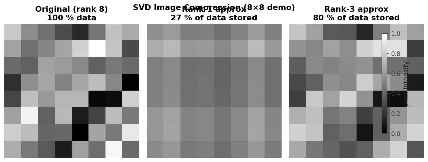SVD low-rank image approximation at varying ranks

1.2 Key Themes

Several themes recur throughout the course and are worth identifying at the outset. The first is the distinction between direct methods and iterative methods. A direct algorithm performs a finite, predetermined sequence of operations and yields the exact solution (in exact arithmetic). Gaussian elimination is a canonical example. An iterative algorithm instead applies the same operations repeatedly to improve an approximate solution until it is “good enough.” Examples include Jacobi iteration, Gauss-Seidel iteration, conjugate gradient, and the PageRank algorithm.

Matrix structure is a second persistent theme. Dense matrices have most or all entries non-zero; they require \( n \times n \) storage and are manipulated in the usual way. Sparse matrices have mostly zero entries, and their non-zero entries may exhibit patterns. Sparsity can be exploited to save both memory and computation, and recognizing or imposing structure is one of the most powerful tools available to practitioners.

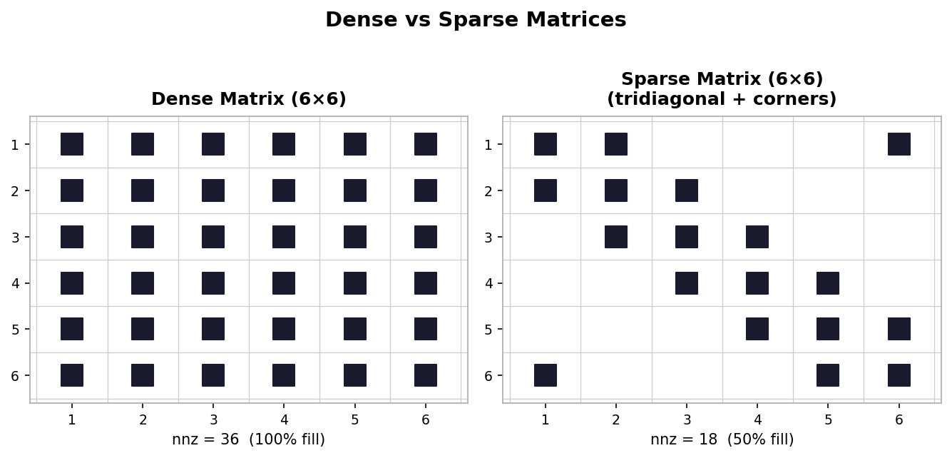Dense (left) vs. sparse tridiagonal (right) matrix nonzero patterns

Matrix factorization is a third central theme. Expressing a matrix \( A \) as a product of simpler matrices, \( A = BCD \), opens up questions about what factorizations exist, what properties they possess, and how those properties can be exploited in algorithm design.

The fourth theme is orthogonality. Vectors \( u, v \in \mathbb{R}^n \) are orthogonal if \( u^T v = 0 \). A square matrix \( Q \in \mathbb{R}^{n \times n} \) is orthogonal if \( Q^T = Q^{-1} \). Orthogonality arises repeatedly throughout many of the algorithms covered in this course.

1.3 Course Topics

The topic of solving linear systems tries to solve \( Ax = b \) for \( x \in \mathbb{R}^n \), where \( A \in \mathbb{R}^{n \times n} \) must be full-rank and \( b \in \mathbb{R}^n \). Although this problem is familiar from earlier courses, solving linear systems efficiently and accurately on large problems in floating-point arithmetic takes substantial effort. Least squares problems also aim to solve \( Ax = b \) but with \( A \in \mathbb{R}^{m \times n} \) and \( b \in \mathbb{R}^m \), seeking the best possible answer when the system may be over- or under-determined. Eigenvalue problems involve finding \( \lambda \) and \( v \) satisfying \( Av = \lambda v \), equivalent to the factorization \( A = Q\Lambda Q^{-1} \). The SVD factors a general \( A \in \mathbb{R}^{m \times n} \) as \( A = U\Sigma V^T \) with orthogonal \( U \) and \( V \) and diagonal non-negative \( \Sigma \), enabling low-rank approximation and many other applications.

---

Linear Algebra Basics

This lecture recaps foundational concepts from linear algebra that will be used throughout the course: vector spaces, bases, dimension, an important interpretation of matrix-vector multiplication, the range, column and row space, null space, rank, nullity, and matrix inverse. It also presents the Sherman-Morrison and Sherman-Morrison-Woodbury formulas for updating a matrix inverse. Much of this material parallels Lecture 1 of Trefethen and Bau, which is recommended as a supplemental read.

2.1 Vector Spaces, Bases, and Dimension

A vector space is a collection of vectors equipped with addition and scalar multiplication operators. An example is \( V = \{v_1, v_2, \ldots, v_k\} \) with \( v_i \in \mathbb{R}^2 \) and the usual operations of component-wise addition and scalar scaling.

A basis \( B \) for a vector space \( V \) is a set of vectors satisfying two conditions: the vectors in \( B \) are linearly independent, and every vector in \( V \) is a linear combination of vectors in \( B \) (i.e., \( B \) spans \( V \). A standard basis for \( \mathbb{R}^3 \) is the set of three unit vectors \( \{e_1, e_2, e_3\} \) with ones in the first, second, and third positions respectively.

The dimension of a vector space \( V \), written \( \dim(V) \), is the number of elements in any basis for \( V \); equivalently, it is the number of linearly independent vectors needed to span \( V \). It is important to note that the dimension of a vector space is not necessarily the same as the dimension of the vectors it contains. For example, the pair of three-dimensional vectors \( \{[1,0,0]^T,\,[0,1,0]^T\} \) spans only a two-dimensional subspace of \( \mathbb{R}^3 \) (the \( xy \)-plane), so \( \dim(V) = 2 \).

2.2 Interpretation of Matrix-Vector Multiplication

Let \( x \in \mathbb{R}^n \) and \( A \in \mathbb{R}^{m \times n} \). The familiar row-times-column interpretation of matrix-vector multiplication yields the product \( b = Ax \) with entries

\[ b_i = \sum_{j=1}^{n} a_{ij} x_j, \quad i = 1, \ldots, m. \]

Here \( a_{ij} \) is the \( (i,j) \) entry of \( A \) and \( x_j \) is the \( j \)-th entry of \( x \). The map \( x \mapsto Ax \) is linear: \( A(x+y) = Ax + Ay \) and \( A(\alpha x) = \alpha Ax \) for any \( x, y \in \mathbb{R}^n \) and \( \alpha \in \mathbb{R} \). Conversely, any linear map from \( \mathbb{R}^n \) to \( \mathbb{R}^m \) can be written as multiplication by an \( m \times n \) matrix.

A more useful interpretation is as a linear combination of columns. If \( a_j \in \mathbb{R}^m \) denotes the \( j \)-th column of \( A \), then

\[ b = Ax = \sum_{j=1}^{n} x_j a_j. \]

This says that \( b \) is a linear combination of the columns of \( A \) with coefficients given by the entries of \( x \). This column-combination view makes it immediately apparent that the range of \( A \) is identical to the column space of \( A \).

The range of \( A \in \mathbb{R}^{m \times n} \) is \( \text{range}(A) = \{y \in \mathbb{R}^m \mid y = Ax,\, x \in \mathbb{R}^n\} \). The column space of \( A \) is the space of all vectors expressible as linear combinations of its columns, and the row space is the analogous span of its rows.

2.3 Null Space, Nullity, and Rank

The null space (or kernel) of \( A \in \mathbb{R}^{m \times n} \) is

\[ \text{null}(A) = \{x \in \mathbb{R}^n \mid Ax = 0\}, \]

the set of all vectors mapped to the zero vector. The zero vector itself always belongs to every null space; interest lies in non-trivial vectors. The dimension of the null space is called the nullity of \( A \), written \( \text{nullity}(A) \). The dimensions of the column and row spaces are both equal to the rank of \( A \), written \( \text{rank}(A) \) — a fundamental result says that column rank always equals row rank. The rank-nullity theorem then gives

\[ \text{rank}(A) + \text{nullity}(A) = n, \]

where \( n \) is the number of columns of \( A \). An \( m \times n \) matrix \( A \) is full rank if \( \text{rank}(A) = \min(m, n) \). When \( A \) is full rank and \( m \geq n \), the map \( x \mapsto Ax \) is one-to-one: distinct inputs produce distinct outputs.

2.4 Matrix Inverse

A square matrix \( A \in \mathbb{R}^{n \times n} \) that is full rank is called invertible or nonsingular. Its inverse \( A^{-1} \) is the unique matrix satisfying \( AA^{-1} = A^{-1}A = I \). For a real square matrix, the following statements are all equivalent: \( A \) is invertible; \( \text{rank}(A) = n \); \( \text{range}(A) = \mathbb{R}^n \); \( \text{null}(A) = \{0\} \); \( A \) has no zero eigenvalues; \( A \) has no zero singular values; and \( \det(A) \neq 0 \).

Several useful matrix inverse identities hold for invertible matrices \( A \) and \( B \): \( (AB)^{-1} = B^{-1}A^{-1} \); \( (A^{-1})^T = (A^T)^{-1} = A^{-T} \); and \( B^{-1} = A^{-1} - B^{-1}(B-A)A^{-1} \). The last identity is verified by multiplying \( B \) on the left: \( B(A^{-1} - B^{-1}(B - A)A^{-1}) = BA^{-1} - (B - A)A^{-1} = BA^{-1} - BA^{-1} + I = I \).

Now suppose we have already computed \( A^{-1} \) and wish to update it after a rank-one modification \( A \to A + uv^T \), where \( u, v \in \mathbb{R}^n \). The Sherman-Morrison formula gives

\[ (A + uv^T)^{-1} = A^{-1} - \frac{A^{-1}uv^T A^{-1}}{1 + v^T A^{-1} u}. \]

This allows updating \( A^{-1} \) without recomputation from scratch; the process is called a rank-one update since \( uv^T \) has rank one. Generalizing to a rank-\( k \) modification, with \( U, V \in \mathbb{R}^{n \times k} \), gives the Sherman-Morrison-Woodbury formula:

\[ (A + UV^T)^{-1} = A^{-1} - A^{-1}U(I + V^T A^{-1} U)^{-1} V^T A^{-1}. \]

A rank-\( k \) modification to \( A \) therefore yields a rank-\( k \) correction to \( A^{-1} \). One can verify this formula by checking that multiplying by \( (A + UV^T) \) recovers the identity.

---

Solving Linear Systems

Many practical problems rely on solving systems of linear equations of the form \( Ax = b \), where \( A \in \mathbb{R}^{n \times n} \), \( b \in \mathbb{R}^n \), and \( x \in \mathbb{R}^n \) is the vector of unknowns. Even algorithms for nonlinear problems often require solving linear systems as substeps. This lecture discusses direct methods based on Gaussian elimination, interpreted through LU factorization and triangular solves, and derives the cost of these algorithms.

3.1 Linear Systems of Equations

To appreciate the scale of modern linear system solves, consider fluid animation. Simulating a fluid for one time-step at a modest resolution of \( 100 \times 100 \times 100 \) cells involves at least one million unknowns, so \( A \) has dimension at least \( 1{,}000{,}000 \times 1{,}000{,}000 \). Animating just ten seconds at 30 frames per second requires solving roughly 300 such problems. Efficient and accurate methods are therefore indispensable.

A key design principle is to avoid constructing \( A^{-1} \) directly: doing so is generally less efficient in terms of operation counts, less accurate due to accumulated round-off error, and more costly in terms of storage (especially for sparse \( A \).

3.2 Gaussian Elimination

Solving \( Ax = b \) via Gaussian elimination is interpreted in three steps. First, factor \( A \) into the product \( A = LU \). Second, perform a forward solve: solve \( Lz = b \) for the intermediate vector \( z \). Third, perform a backward solve: solve \( Ux = z \) for \( x \). Here \( L \) is lower triangular (zero entries above the main diagonal) and \( U \) is upper triangular (zero entries below the main diagonal). When equations in \( Ax = b \) must be rearranged to avoid zero pivots, one uses the permuted LU factorization \( PA = LU \), where \( P \) is a permutation matrix (the identity matrix with rows rearranged), and solves \( PAx = Pb \) instead.

LU Factorization. The algorithm proceeds one column at a time, subtracting appropriate multiples of each pivot row from the rows below it to introduce zeros in the sub-diagonal entries of that column. The multiplicative factors used to zero out entry \( a_{ik} \) are stored in place of those zeros and constitute the entries of \( L \). The resulting \( L \) is unit lower triangular (diagonal entries are all 1). The in-place pseudocode iterates over each column \( k = 1, \ldots, n \); for each row \( i > k \) it computes the multiplier \( \text{mult} = a_{ik}/a_{kk} \), stores it at position \( a_{ik} \) (where a zero would otherwise go), and subtracts \( \text{mult} \times \) the current pivot row from row \( i \).

Triangular Solves. Substituting \( A = LU \) into \( Ax = b \) gives \( L(Ux) = b \). Setting \( z = Ux \), one first solves \( Lz = b \) (forward substitution, working from top to bottom through the equations) and then \( Ux = z \) (backward substitution, working from bottom to top). These two solves are far more efficient than solving the original system because the triangular structure means each unknown is determined by one simple equation once its predecessors are known.

The forward substitution algorithm initializes \( z_i = b_i \) and subtracts the already-solved \( z_j \) values weighted by \( l_{ij} \) for \( j < i \). The backward substitution algorithm initializes \( x_i = z_i \), subtracts the already-solved \( x_j \) values weighted by \( u_{ij} \) for \( j > i \), and divides by \( u_{ii} \). Both algorithms assume non-zero diagonal entries; zero or near-zero pivot entries cause problems that are addressed through pivoting (discussed in Week 3 on stability of factorizations).

3.3 Cost of Gaussian Elimination

The cost of an algorithm is measured in flops (floating-point operations: adds, subtracts, multiplies, and divides). Note that “flops” here denotes a count, not a rate. Actual hardware timing depends on factors such as fused-multiply-add operations, but flop counting gives a reliable asymptotic picture.

For the LU factorization, the dominant cost comes from the innermost loop of the algorithm. Counting the multiplications and subtractions across all three nested loops and summing using standard identities for \( \sum k \) and \( \sum k^2 \) yields a total of

\[ \frac{2n^3}{3} + O(n^2) = O(n^3) \]

flops for factorization. Each triangular solve costs \( n^2 + O(n) = O(n^2) \) flops, so the total cost of Gaussian elimination is

\[ \frac{2n^3}{3} + O(n^2) + 2(n^2 + O(n)) = O(n^3). \]

The LU factorization dominates for large \( n \). This has an important practical consequence: once \( L \) and \( U \) are available, solving with a different right-hand side \( b \) costs only \( O(n^2) \) additional flops.

Constructing \( A^{-1} \). If the explicit inverse is genuinely needed, one can factor \( A = LU \) once and then solve \( LU v_k = e_k \) for each standard basis vector \( e_k \); the columns \( v_k \) assemble to give \( A^{-1} \). Each additional right-hand side costs only \( O(n^2) \) flops. Nonetheless, most numerical algorithms avoid constructing \( A^{-1} \) for the reasons outlined in Section 3.1.

Worked Example: LU Factorization and Solve

This example walks through solving \( Ax = b \) for a specific \( 3 \times 3 \) system by computing the LU factorization and then performing forward and backward substitution.

The first step is to factor \( A \) into its lower and upper triangular components \( L \) and \( U \). The process follows exactly the steps of Gaussian elimination. To zero out the entry in row 2, column 1, one replaces row 2 with row 2 minus 1 times row 1. This leaves row 1 unchanged and produces a zero in the \( (2,1) \) position. For example, if \( a_{21} = 1 \) and \( a_{11} = 1 \), the multiplier is 1 and the updated entries in row 2 become \( 1 - 1 = 0 \), \( -2 - 1 = -3 \), and \( 2 - 1 = 1 \). Row 3 remains unchanged after this first step.

In the next step, zeroing out position \( (3,1) \) requires replacing row 3 with row 3 minus 1 times row 1. Rows 1 and 2 remain unchanged. The result introduces a zero in position \( (3,1) \) and updates the remaining entries: \( 2 - 1 = 1 \) and \( -1 - 1 = -2 \).

The final elimination step zeros out position \( (3,2) \) by replacing row 3 with row 3 minus \( -\tfrac{1}{3} \) times row 2. The pivot row entry is \( -3 \), giving a multiplier of \( -\tfrac{1}{3} \). The new entry in position \( (3,3) \) becomes \( -2 - (-\tfrac{1}{3}) \cdot 1 = -2 + \tfrac{1}{3} = -\tfrac{5}{3} \). This final matrix is \( U \), the upper triangular factor.

The matrix \( L \) is built from the multiplicative factors used at each step. It is unit lower triangular, with ones on the diagonal. The three multipliers used were 1, 1, and \( -\tfrac{1}{3} \), placed in the positions they zeroed out.

With \( L \) and \( U \) in hand, the forward solve \( Lz = b \) begins at the top equation. The first equation gives \( z_1 = 0 \) immediately. The second equation gives \( z_1 + z_2 = 4 \), so \( z_2 = 4 \). The third equation gives \( z_1 - \tfrac{1}{3}z_2 + z_3 = 2 \), which becomes \( 0 - \tfrac{4}{3} + z_3 = 2 \) and so \( z_3 = \tfrac{6}{3} + \tfrac{4}{3} = \tfrac{10}{3} \).

The backward solve \( Ux = z \) starts at the bottom equation: \( -\tfrac{5}{3} x_3 = \tfrac{10}{3} \), giving \( x_3 = -2 \). The second equation from the bottom gives \( -3x_2 + x_3 = 4 \), so \( -3x_2 = 4 + 2 = 6 \) and \( x_2 = -2 \). The top equation gives \( x_1 + x_2 + x_3 = 0 \), so \( x_1 = -x_2 - x_3 = 2 + 2 = 4 \). The final solution is \( x = [4,\,-2,\,-2]^T \).

Worked Example: Cost of LU Factorization

This example derives the leading-order flop count for LU factorization by carefully summing operations across all three nested loops.

The innermost loop body performs two flops: one subtraction and one multiplication. Immediately outside the innermost loop, there is one division, contributing one additional flop per iteration of the middle loop. The total cost is the sum of all these flops over all iterations of all three loops.

Writing this as a triple sum, the cost equals \( \sum_{k=1}^{n} \sum_{i=k+1}^{n} \left(1 + \sum_{j=k+1}^{n} 2\right) \). Evaluating the innermost sum first, \( \sum_{j=k+1}^{n} 2 = 2(n-k) \), by the basic identity that summing the constant 1 from \( r \) to \( s \) gives \( s - r + 1 \). Combining with the division term yields the factor \( 1 + 2(n-k) = 1 + 2n - 2k \) per middle-loop iteration.

Summing over \( i \) from \( k+1 \) to \( n \) gives \( (n-k)(1 + 2n - 2k) \). Expanding the product yields terms of order constant, linear, and quadratic in \( k \). The final sum over \( k \) from 1 to \( n \) is evaluated using the known identities \( \sum_{k=1}^{n} k = \frac{n(n+1)}{2} \) and \( \sum_{k=1}^{n} k^2 = \frac{n(n+1)(2n+1)}{6} \). Substituting these and simplifying all terms produces the total cost

\[ \frac{2}{3}n^3 - \frac{1}{2}n^2 - \frac{1}{6}n = \frac{2n^3}{3} + O(n^2), \]

confirming the \( O(n^3) \) scaling stated in the lecture notes. The leading coefficient \( \tfrac{2}{3} \) will be seen to be exactly twice the leading coefficient of Cholesky factorization, reflecting the symmetry savings exploited in that method.

Worked Example: Partial Pivoting

This example demonstrates solving \( Ax = b \) using LU factorization with partial pivoting. The process factors \( A \) such that \( PA = LU \), where \( P \) is a permutation matrix. The resulting system becomes \( PAx = Pb \), equivalently \( LUx = \tilde{b} \) where \( \tilde{b} = Pb \), and this is solved with the usual two triangular solves.

The first step is to factor \( A \). With partial pivoting, one examines the magnitude of entries in the first column to select the pivot. Suppose the third entry has the largest magnitude (for example, 2 is greater than 1), so rows 1 and 3 must be swapped. The first permutation matrix \( P_1 \) is the identity matrix with rows 1 and 3 swapped. After applying \( P_1 \), the permuted matrix \( P_1 A \) has the largest entry on the diagonal of the first column, making it a safe pivot.

Row subtractions then zero out the two entries below the pivot. Both rows 2 and 3 are updated by subtracting one-half of row 1 (the multiplier \( \tfrac{1}{2} \) follows from dividing each sub-diagonal entry by the pivot 2). This produces zeros in the first column and updates the remaining entries: for example, the \( (2,2) \) entry becomes \( -1 - \tfrac{1}{2}(3) = -\tfrac{5}{2} \) and the \( (2,3) \) entry becomes \( 1 - \tfrac{1}{2}(-1) = \tfrac{3}{2} \).

After the first elimination stage, the two candidate pivot entries in the second column are equal in magnitude, so no row swap is needed. The second permutation matrix \( P_2 \) is therefore just the identity. The final elimination step replaces row 3 with row 3 minus 1 times row 2, zeroing the \( (3,2) \) entry and updating \( (3,3) \) to \( \tfrac{5}{2} - \tfrac{3}{2} = 1 \). The resulting upper triangular matrix is \( U \).

The total permutation matrix is \( P = P_2 P_1 = P_1 \) since \( P_2 = I \), giving the matrix that swaps rows 1 and 3. The lower triangular factor \( L \) is unit lower triangular with the three multipliers \( \tfrac{1}{2} \), \( \tfrac{1}{2} \), and 1 placed in the appropriate sub-diagonal positions.

To solve for \( x \), one first permutes the right-hand side: \( \tilde{b} = Pb \), which swaps the first and third entries of \( b = [4,1,2]^T \) to give \( \tilde{b} = [2,1,4]^T \). The forward solve \( Lz = \tilde{b} \) then gives \( z = [4, -1, 1]^T \), and the backward solve \( Ux = z \) yields the final answer \( x = [1, 1, 1]^T \).

---

Special Linear Systems

This lecture addresses a central question: can \( Ax = b \) be solved more efficiently by exploiting properties of \( A \)? The answer is yes. The common matrix types considered in this course are symmetric, positive definite (PD), symmetric positive definite (SPD), banded, tridiagonal, and general sparse. This lecture covers the first three types, which lead to the \( LDL^T \) factorization for symmetric matrices and the Cholesky factorization for SPD matrices.

4.1 Symmetric Matrices

A symmetric matrix satisfies \( A = A^T \); symmetry requires the matrix to be square. A general LU-like factorization exists for any matrix possessing an LU factorization, as stated in Theorem 4.1: there exist unique unit lower triangular matrices \( L, M \) and a diagonal matrix \( D \) such that \( A = LDM^T \). The proof constructs \( D = \text{diag}(u_{11}, u_{22}, \ldots, u_{nn}) \) from the diagonal of \( U \) and sets \( M^T = D^{-1}U \), so that dividing rows of \( U \) by the corresponding diagonal entry makes the diagonal of \( M^T \) all ones, and \( M \) becomes unit lower triangular.

Unfortunately the flop count of \( LDM^T \) is essentially the same as a plain LU factorization. However, if \( A \) is symmetric, then Theorem 4.2 guarantees that \( M = L \), giving the \( LDL^T \) factorization \( A = LDL^T \). Since \( M = L \) there is no need to compute redundant entries; roughly half the cost of a plain LU factorization is saved.

The proof of \( M = L \) proceeds by considering the matrix \( M^{-1}AM^{-T} \), which is symmetric (as \( A \) is symmetric) and evaluates to \( M^{-1}L D \). The product \( M^{-1}L \) is lower triangular (product of two lower triangular matrices), so \( M^{-1}LD \) is lower triangular. But it is also symmetric, and the only lower triangular symmetric matrix is a diagonal matrix. Since both \( L \) and \( M \) are unit lower triangular, \( M^{-1}L \) is also unit triangular and diagonal, hence the identity, so \( M = L \).

4.2 Positive Definiteness

A matrix \( A \in \mathbb{R}^{n \times n} \) is positive definite (PD) if \( x^T Ax > 0 \) for all \( x \in \mathbb{R}^n \), \( x \neq 0 \). This generalizes the notion of positivity for scalars: \( a \in \mathbb{R} \) is positive if \( xax > 0 \) for all \( x \neq 0 \). The function \( f(x) = x^T Ax \) is quadratic with \( A \) as its coefficient matrix; positive definiteness is equivalent to asking whether \( f \) is convex (a bowl shape with a unique minimum). Positive definiteness implies invertibility and strictly positive eigenvalues.

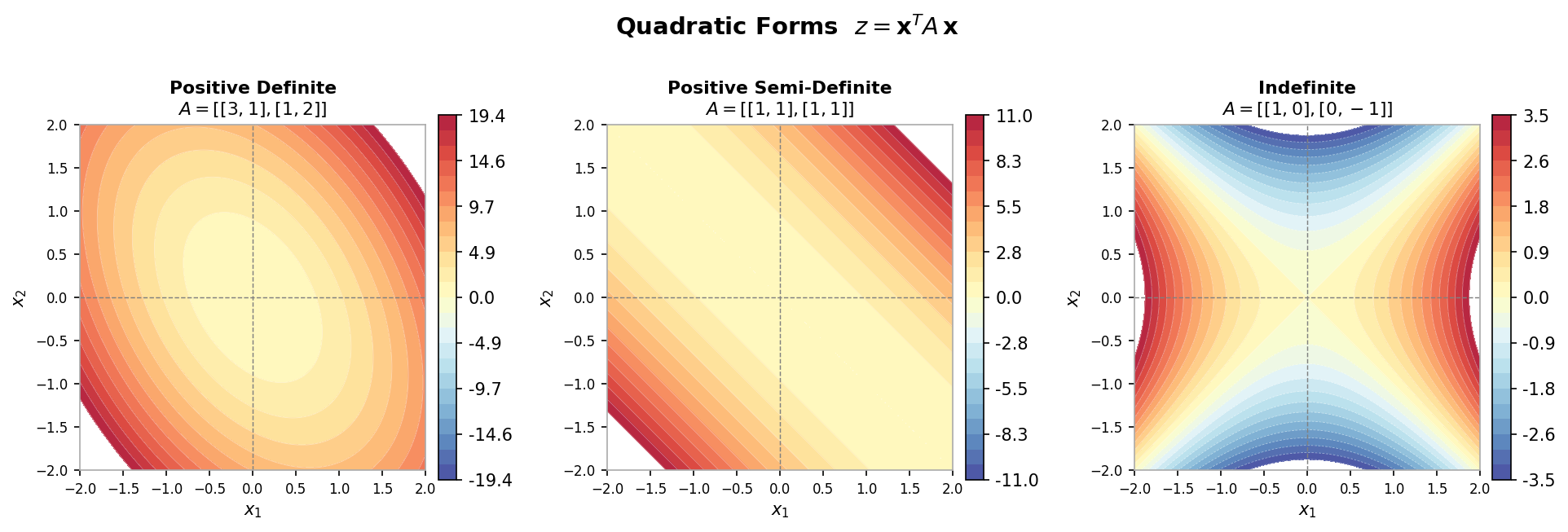Contour plots of positive definite, positive semi-definite, and indefinite quadratic forms

A fundamental result (Theorem 4.3) states that if \( A \in \mathbb{R}^{n \times n} \) is PD and \( X \in \mathbb{R}^{n \times k} \) has rank \( k \leq n \), then \( B = X^T AX \) is also PD. The proof sets \( x = Xz \) for any \( z \neq 0 \): since \( X \) has rank \( k \), its null space contains only the zero vector (by the rank-nullity theorem), so \( x = Xz \neq 0 \) whenever \( z \neq 0 \), and then \( z^T B z = (Xz)^T A (Xz) = x^T Ax > 0 \) since \( A \) is PD.

A principal submatrix is constructed by deleting rows and their corresponding columns from a matrix. Two corollaries follow from Theorem 4.3. First, if \( A \) is PD then all its principal submatrices are also PD (one can design identity-like matrices \( X \) to “pick out” any principal submatrix via \( X^T AX \). In particular, every diagonal entry of a PD matrix is strictly positive. Second, if \( A \) is PD, then the diagonal matrix \( D \) in the factorization \( A = LDM^T \) has strictly positive entries. This follows by taking \( X = L^{-T} \) and applying Corollary 4.1 to the principal submatrix argument.

4.3 Symmetric Positive Definite Matrices

A symmetric positive definite (SPD) matrix \( A \) satisfies both \( A = A^T \) and \( x^T Ax > 0 \) for all \( x \neq 0 \). Theorem 4.4 states that if \( A \) is SPD, there exists a unique lower triangular matrix \( G \) with positive diagonal entries such that \( A = GG^T \). This is the Cholesky factorization and \( G \) is the Cholesky factor.

The existence proof uses the \( LDL^T \) factorization guaranteed by symmetry: since \( A \) is PD, the diagonal entries of \( D \) are all positive. One can therefore define \( D^{1/2} = \text{diag}(\sqrt{d_1}, \ldots, \sqrt{d_n}) \) and set \( G = LD^{1/2} \), which is lower triangular with positive diagonal. Then \( GG^T = LD^{1/2}(LD^{1/2})^T = LD^{1/2}D^{1/2}L^T = LDL^T = A \).

Constructing the Cholesky Factor. The algorithm works recursively. Partition \( A \) as

\[ A = \begin{pmatrix} \alpha & v^T \\ v & B \end{pmatrix}, \]

where \( \alpha = a_{11} \in \mathbb{R} \), \( v = a_{2:n,1} \in \mathbb{R}^{n-1} \), and \( B = a_{2:n,2:n} \in \mathbb{R}^{(n-1) \times (n-1)} \). The first column of \( G \) is determined by comparing block forms of \( GG^T \) with \( A \):

\[ g_{11} = \sqrt{\alpha}, \quad G_{21} = \frac{v}{\sqrt{\alpha}}, \quad G_{22}G_{22}^T = B - \frac{vv^T}{\alpha}. \]

The algorithm then recursively applies Cholesky factorization to the Schur complement \( B - vv^T/\alpha \), which is itself SPD (one verifies this using Theorem 4.3 with the full-rank matrix \( X = [1, -v^T/\alpha;\, 0, I] \). The recursion eliminates one row and column at a time until the entire lower triangular factor \( G \) is assembled.

Cost of Cholesky Factorization. The in-place algorithm (Algorithm 4.1) exploits symmetry by working only on sub-diagonal entries, iterating over the diagonal entry, the column below it, and the lower-right block update. Focusing on the innermost doubly-nested loop (which contributes one subtraction and one multiplication per iteration), the total flop count is

\[ \sum_{k=1}^{n} \sum_{j=k+1}^{n} \sum_{i=j}^{n} 2 = \frac{n^3}{3} + O(n^2), \]

which is exactly half the cost of LU factorization (\( \frac{2n^3}{3} + O(n^2) \) flops). The square roots and column divisions contribute only \( O(n^2) \) and \( O(n) \) terms respectively and are dominated by the lower-right block updates.

Worked Example: Cholesky Factorization

This example walks through computing the Cholesky factorization of a specific SPD matrix step by step, illustrating the recursive structure of the algorithm.

Consider a \( 3 \times 3 \) SPD matrix \( A \). The first step is to identify \( \alpha \), \( v \), and \( B \) in the block decomposition of \( A \). The top-left corner gives \( \alpha = 9 \), the column below it gives \( v = [3, 0]^T \), and the lower-right submatrix gives \( B = \begin{pmatrix} 5 & 2 \\ 2 & 17 \end{pmatrix} \).

Computing the first column of \( G \): the diagonal entry is \( \sqrt{\alpha} = \sqrt{9} = 3 \); the entries below the diagonal are \( v/\sqrt{\alpha} = [3/3, 0/3]^T = [1, 0]^T \). The Schur complement is \( B - vv^T/\alpha = \begin{pmatrix} 5 & 2 \\ 2 & 17 \end{pmatrix} - \frac{1}{9}\begin{pmatrix} 9 & 0 \\ 0 & 0 \end{pmatrix} = \begin{pmatrix} 4 & 2 \\ 2 & 17 \end{pmatrix} \).

After the first stage, the factorization has its first column of \( G \) as \( [3, 1, 0]^T \), and the algorithm now recurses on the \( 2 \times 2 \) Schur complement.

For the second recursion, the sub-matrix is \( \begin{pmatrix} 4 & 2 \\ 2 & 17 \end{pmatrix} \). Identifying the block components: \( \alpha = 4 \), \( v = [2] \), \( B = [17] \). The diagonal entry of the second column of \( G \) is \( \sqrt{4} = 2 \); the entry below is \( 2/2 = 1 \). The Schur complement is \( 17 - (1/4) \cdot 4 = 17 - 4 \cdot (4/4) = 17 - 4 = 16 \). Wait — more carefully: \( B - vv^T/\alpha = 17 - 2^2/4 = 17 - 1 = 16 \). The second column of \( G \) contributes \( [2, 1]^T \) in the appropriate positions.

The third and final recursion operates on the \( 1 \times 1 \) Schur complement \( [16] \). Its Cholesky factor is simply \( \sqrt{16} = 4 \), which becomes the third diagonal entry of \( G \).

Assembling all columns, the Cholesky factor is

\[ G = \begin{pmatrix} 3 & 0 & 0 \\ 1 & 2 & 0 \\ 0 & 1 & 4 \end{pmatrix}. \]

One can verify that \( GG^T = A \).

Worked Example: Cost of Cholesky Factorization

This example derives the exact leading-order flop count for Cholesky factorization, confirming that it is half that of LU factorization.

The algorithm has three nested loops: the outermost over \( k = 1 \) to \( n \), a middle loop over \( j = k+1 \) to \( n \), and an innermost loop over \( i = j \) to \( n \). Inside the innermost loop there are two flops (one subtraction, one multiplication). The division outside the innermost loop contributes only an \( O(n^2) \) term, and the square root outside the middle loop contributes only an \( O(n) \) term.

Focusing on the dominant innermost loop, the total cost is

\[ 2 \sum_{k=1}^{n} \sum_{j=k+1}^{n} \sum_{i=j}^{n} 1. \]

Evaluating the innermost sum using the formula \( \sum_{i=j}^{n} 1 = n - j + 1 \), then splitting the middle sum into constant and linear parts in \( j \), one applies the identities for summing 1 and for summing the index itself (using a dummy variable shift since the index does not start at 1). After carrying through the algebra, the outer sum over \( k \) is evaluated using the known identities for \( \sum k \) and \( \sum k^2 \). The final result is

\[ \frac{n^3}{3} - \frac{n}{3} = \frac{n^3}{3} + O(n), \]

confirming that the leading-order cost is \( \frac{n^3}{3} \) flops — precisely half the \( \frac{2n^3}{3} \) flops required by LU factorization. This savings arises directly from exploiting the symmetry of an SPD matrix to avoid redundant computation on the upper triangle.

---

Special Linear Systems (Part 2)

This lecture continues the theme of exploiting matrix structure to solve \( Ax = b \) more efficiently. The first three matrix types — symmetric, positive definite, and symmetric positive definite — were treated in Lecture 4. This lecture covers the remaining three common types: banded matrices, tridiagonal matrices (a special case of banded), and general sparse matrices.

5.1 Banded Matrices

Banded matrices have non-zero entries only in “bands” adjacent to the main diagonal; all entries sufficiently far from the diagonal are zero. Formally, the matrix \( A = [a_{ij}] \) has upper bandwidth \( q \) if \( a_{ij} = 0 \) for \( j > i + q \), and lower bandwidth \( p \) if \( a_{ij} = 0 \) for \( i > j + p \). Common special cases include diagonal matrices (\( p = q = 0 \), upper triangular (\( p = 0 \), \( q = n-1 \), lower triangular (\( p = m-1 \), \( q = 0 \), tridiagonal (\( p = q = 1 \), upper and lower bidiagonal (\( (p,q) = (0,1) \) and \( (1,0) \), and upper and lower Hessenberg (\( (p,q) = (1, n-1) \) and \( (m-1, 1) \).

An important structural property of banded matrices is preserved under factorization: if \( A = LU \), \( A \) has upper bandwidth \( q \) and lower bandwidth \( p \), then \( U \) has upper bandwidth \( q \) and \( L \) has lower bandwidth \( p \). The same bandwidth preservation holds for the \( LDL^T \) and Cholesky \( GG^T \) factorizations.

Cost of Banded LU Factorization. The banded LU factorization algorithm (Algorithm 5.1) restricts its inner loops to the non-zero bands: for each pivot column \( k \), the row loop runs only from \( k+1 \) to \( \min(k+p, n) \) and the column loop only from \( k+1 \) to \( \min(k+q, n) \). When the bandwidths are small relative to \( n \) (i.e., \( n \gg p \) and \( n \gg q \), the cost is approximately \( 2npq \) flops, dramatically less than the \( \frac{2n^3}{3} \) flops of the naive full implementation that would touch the zero entries. For example, with \( n = 300 \), \( p = 2 \), \( q = 2 \): naive LU requires approximately 18,000,000 flops, while banded LU requires only approximately 2,400 flops. For tridiagonal matrices (\( p = q = 1 \), the flop count reduces to \( O(n) \).

Tridiagonal \( LDL^T \) Factorization. When a symmetric tridiagonal matrix \( A \) is factored as \( A = LDL^T \), the factors inherit the tridiagonal structure: \( L \) is unit lower bidiagonal with sub-diagonal entries \( e_1, \ldots, e_{n-1} \), and \( D = \text{diag}(d_1, \ldots, d_n) \). Expanding the product \( (LDL^T)_{kk} = e_{k-1}^2 d_{k-1} + d_k \) and \( (LDL^T)_{k,k-1} = e_{k-1} d_{k-1} \) yields explicit recurrence relations:

\[ d_1 = a_{11}, \quad \text{for } k = 2, \ldots, n: \quad e_{k-1} = \frac{a_{k,k-1}}{d_{k-1}}, \quad d_k = a_{kk} - e_{k-1} a_{k,k-1}. \]

This algorithm requires only \( O(n) \) flops and \( O(n) \) storage, making it optimal for tridiagonal systems. Once \( L \) and \( D \) are available, solving \( LDL^T x = b \) via forward and backward substitution also costs only \( O(n) \) flops.

5.2 General Sparse Matrices

Patterns other than simple bands also arise frequently. General sparse matrices contain mostly zero entries but with non-zeros possibly scattered across the matrix beyond just diagonal bands. For many practical problems, the number of non-zeros per row is bounded by a small constant, so the total number of non-zeros is \( O(n) \); one naturally wants to store and operate on only the non-zero entries.

Various storage formats (data structures) exist for sparse matrices. The simplest approach uses a vector of \( (i, j, \text{value}) \) triplets, one per non-zero, but this is inefficient. A more common structure is Compressed Row Storage (CRS), also known as Compressed Sparse Row (CSR): it uses an array of non-zero values (val) of length equal to the number of non-zeros (nnz), an array of column indices (colInd) of length nnz, and an array of row-start pointers (rowPtr) of length equal to the number of rows.

Fill-in During Factorization. For LU factorization of a sparse matrix, the key computational step is the row subtraction \( a_{ij} \leftarrow a_{ij} - a_{ik} a_{kj}/a_{kk} \). Since most entries are zero, algorithms skip operating on them. However, even if \( A \) is sparse, its factorization may not be, because row subtractions can turn zero entries into non-zeros. This phenomenon is called fill-in.

A classic example is the arrow matrix: a matrix with a dense first row, a dense first column, and diagonal entries elsewhere. The LU factors of such a matrix are fully dense in the corresponding triangles, meaning all potential fill-in positions become non-zero. The key intuition is that one must reorder the system of equations to avoid or minimize fill-in. A matrix reordering permutes the rows and columns to yield a matrix whose LU factorization suffers no (or minimal) fill-in. For the arrow matrix, if the dense row and column are moved to the last position rather than the first, the LU factors are again sparse. Matrix reorderings are discussed in detail starting in Lecture 8.

---

Finite Differences for Modelling Heat Conduction

This lecture covers an important application of solving linear systems: the numerical solution of partial differential equations (PDEs). PDEs involve multivariable functions and their partial derivatives and describe numerous physical phenomena including electromagnetism, fluid flow, sound propagation, financial problems, solid mechanics, and quantum mechanics. Finite difference, finite volume, and finite element methods discretize PDEs and produce sparse linear systems. This lecture introduces finite differences for the Poisson equation, which models heat conduction.

6.1 Heat Conduction

The heat distribution in a uniform material at equilibrium is modelled by the Poisson equation:

\[ -\left(\frac{\partial^2 T}{\partial x^2} + \frac{\partial^2 T}{\partial y^2} + \frac{\partial^2 T}{\partial z^2}\right) = f, \quad \text{equivalently} \quad -\Delta T = f, \]

where \( x, y, z \) are spatial coordinates, \( T(x, y, z) \) is the temperature field, \( f(x, y, z) \) is a given heat source function, and \( \Delta = \frac{\partial^2}{\partial x^2} + \frac{\partial^2}{\partial y^2} + \frac{\partial^2}{\partial z^2} \) is the Laplacian operator.

1D Example. Consider the one-dimensional problem

\[ -\frac{\partial^2 T}{\partial x^2} = f \quad \text{on } (0, 1), \qquad T(0) = 0, \quad T(1) = 0. \]

The second and third conditions are the boundary conditions, prescribing zero temperature at both ends. To find an approximate numerical solution, the approach is to first discretize the domain into finite subintervals and then approximate the spatial derivative with finite differences.

Discretizing the 1D domain means defining \( n+2 \) evenly spaced gridpoints \( 0 = x_0 < x_1 < x_2 < \cdots < x_n < x_{n+1} = 1 \). The grid spacing is \( h = x_i - x_{i-1} = \frac{1}{n+1} \). The numerical approximation of the exact solution at gridpoint \( x_i \) is denoted \( T_i \). Since the boundary conditions fix \( T_0 = 0 \) and \( T_{n+1} = 0 \), only the \( n \) interior values \( T_1, T_2, \ldots, T_n \) are unknowns. These are the active gridpoints.

The centered finite difference approximation of the second derivative is

\[ \frac{\partial^2 T}{\partial x^2}(x_i) \approx \frac{T_{i+1} - 2T_i + T_{i-1}}{h^2}. \]

Applying this to the PDE at each active gridpoint gives one equation per interior gridpoint:

\[ -\frac{T_{i+1} - 2T_i + T_{i-1}}{h^2} = f_i, \quad i = 1, \ldots, n. \]

Each equation relates \( T_i \) to its two neighbors \( T_{i-1} \) and \( T_{i+1} \). Assembling all \( n \) equations into matrix form yields

\[ \frac{1}{h^2} \begin{pmatrix} 2 & -1 & & & \\ -1 & 2 & -1 & & \\ & \ddots & \ddots & \ddots & \\ & & -1 & 2 & -1 \\ & & & -1 & 2 \end{pmatrix} \begin{pmatrix} T_1 \\ T_2 \\ \vdots \\ T_{n-1} \\ T_n \end{pmatrix} = \begin{pmatrix} f_1 \\ f_2 \\ \vdots \\ f_{n-1} \\ f_n \end{pmatrix}. \]

The resulting matrix is symmetric and tridiagonal (a banded matrix with \( p = q = 1 \), and the system can be solved using the banded LU or Cholesky algorithms in \( O(n) \) flops.

Heat Conduction in a 2D Plate. For a two-dimensional rectangular plate with zero temperature on all boundaries, the 2D Poisson equation at interior gridpoint \( (x_i, y_j) \) is discretized by approximating the second derivative in each axis separately and summing:

\[ \frac{4T_{i,j} - T_{i+1,j} - T_{i-1,j} - T_{i,j+1} - T_{i,j-1}}{h^2} = f_{i,j}. \]

This is the discrete 2D Poisson equation. The finite difference stencil is a convenient visual representation centered at each gridpoint showing the weights of the five terms: \( 4/h^2 \) at the center, \( -1/h^2 \) at each of the four neighbors.

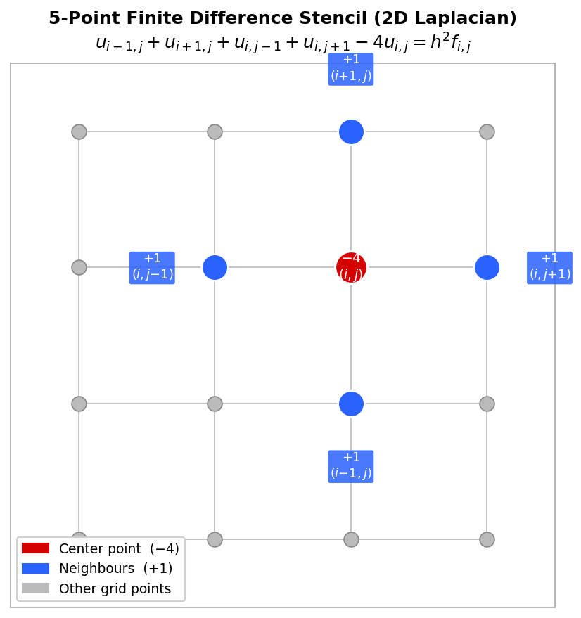Five-point finite difference stencil with coefficients labelled

To form a matrix equation, the 2D indices \( (i,j) \) must be flattened to a 1D index. Natural rowwise ordering numbers gridpoints along the \( x \)-axis first and then along the \( y \)-axis: the mapping is \( k = i + (j-1) \times m \) for an \( m \times m \) grid of interior points. With this ordering and an \( m^2 \times m^2 \) system of equations, the resulting matrix has five bands:

• 1 main diagonal band (with entries 4),
• 2 adjacent off-diagonal bands (with entries \( -1 \),
• 2 further off-diagonal bands separated by \( m \) positions (with entries \( -1 \).

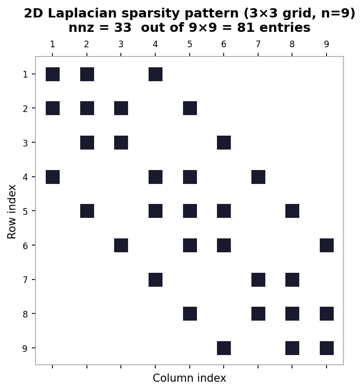Sparsity pattern of the 2D Laplacian matrix for a 3×3 interior grid

The matrix is symmetric, and its graph recovers the underlying 2D grid structure. Other types of PDE problems, discretizations, and geometries — such as triangular meshes for finite volume discretization of flow around an airfoil — give rise to different matrix structures and properties. This lecture focused on the equilibrium (steady-state) heat equation; the time-dependent heat equation gives rise to similar but time-evolving linear systems.

Worked Example: 1D Poisson Matrix Equation

This example derives the matrix form of the discrete 1D Poisson equation for a specific case with six gridpoints (\( x_0 \) to \( x_5 \), so that \( n+1 = 5 \) and the grid spacing is \( h = 1/5 \). The boundaries fix \( T_0 = 0 \) and \( T_5 = 0 \), leaving four active gridpoints \( T_1, T_2, T_3, T_4 \).

To build the matrix equation, one writes out the discrete equation for each active gridpoint. For \( i = 1 \), the discrete equation gives \( (-T_2 + 2T_1 - T_0)/h^2 = f_1 \); since \( T_0 = 0 \) the boundary term drops out. For \( i = 2 \), one gets \( (-T_3 + 2T_2 - T_1)/h^2 = f_2 \). For \( i = 3 \), one gets \( (-T_4 + 2T_3 - T_2)/h^2 = f_3 \). For \( i = 4 \) (the last active point), one gets \( (-T_5 + 2T_4 - T_3)/h^2 = f_4 \); since \( T_5 = 0 \) the boundary term drops out on this end as well.

Writing these four equations in matrix form, with \( 1/h^2 \) factored outside, gives a coefficient matrix with 2 on the main diagonal, \( -1 \) on the two adjacent off-diagonals, and zeros elsewhere. Examining the first row one sees the pattern \( [2, -1, 0, 0] \), the second row \( [-1, 2, -1, 0] \), the third \( [0, -1, 2, -1] \), and the fourth \( [0, 0, -1, 2] \). This is the familiar symmetric tridiagonal structure. The right-hand side vector is \( [f_1, f_2, f_3, f_4]^T \), the source values at the active gridpoints.

Worked Example: 2D Poisson Matrix Equation

This example illustrates building the 2D Poisson matrix equation and the index-flattening procedure for the specific case \( m = 4 \) (a \( 4 \times 4 \) grid of interior points, so \( m^2 = 16 \) unknowns), with zero boundary temperatures. The natural rowwise ordering flattens 2D indices \( (i, j) \) to 1D indices \( k \) using \( k = i + (j-1) \times m \).

As a first example, consider the equation for interior point \( T_{2,2} \) (\( i=2 \), \( j=2 \). The discrete Poisson equation gives \( (1/h^2)(4T_{2,2} - T_{3,2} - T_{1,2} - T_{2,3} - T_{2,1}) = f_{2,2} \). Flattening the indices: the center \( (2,2) \) maps to \( k = 2 + (2-1) \times 4 = 6 \); the neighbor \( (3,2) \) maps to \( k = 3 + 4 = 7 \); \( (1,2) \) maps to \( k = 1 + 4 = 5 \); \( (2,3) \) maps to \( k = 2 + 8 = 10 \); and \( (2,1) \) maps to \( k = 2 + 0 = 2 \). In the 1D-indexed system this corresponds to row 6: the entry \( (6,6) = 4 \) and entries \( (6,7) \), \( (6,5) \), \( (6,10) \), \( (6,2) \) are all \( -1 \).

As a second example, consider the equation for \( T_{2,4} \) (\( i=2 \), \( j=4 \). The discrete Poisson equation gives \( (1/h^2)(4T_{2,4} - T_{3,4} - T_{1,4} - T_{2,5} - T_{2,3}) = f_{2,4} \). Since \( m = 4 \), the point \( (2,5) \) lies on the boundary, so \( T_{2,5} = 0 \) and that term disappears. Flattening the remaining indices: center \( (2,4) \) maps to \( k = 2 + 3 \times 4 = 14 \); \( (3,4) \) maps to \( 3 + 12 = 15 \); \( (1,4) \) maps to \( 1 + 12 = 13 \); and \( (2,3) \) maps to \( 2 + 2 \times 4 = 10 \). Row 14 of the matrix therefore has a 4 on the diagonal and \( -1 \) entries in columns 15, 13, and 10 — only three off-diagonal entries instead of four, reflecting the missing boundary neighbor.

The general matrix from the 2D Poisson equation with natural ordering has blocks of tridiagonal structure along the main diagonal (from the \( x \)-direction coupling) and blocks of \( -1 \)s on the off-block-diagonals (from the \( y \)-direction coupling), resulting in a banded symmetric matrix with bandwidth \( m \).

---

Graph Structure of Matrices

This lecture considers the graph representation of (symmetric) matrices and examines how fill-in during factorization is related to the graph structure. Since fill-in increases both storage and computational costs, understanding and minimizing it is central to efficient sparse linear algebra. The graph perspective provides an intuitive framework for analyzing and designing matrix reordering algorithms.

7.1 Graph Structure of Matrices

Given a matrix \( A \), one can construct an associated directed graph \( G(A) \). The graph has one node \( i \) for each row \( i \) of \( A \), and a directed edge \( (i \to j) \) exists whenever the matrix entry \( a_{ij} \neq 0 \) (for \( i \neq j \). For symmetric matrices, edges are undirected: \( i \leftrightarrow j \). Formally, for a square matrix \( A \in \mathbb{R}^{n \times n} \), the associated graph \( G = (V, E) \) has nodes \( i \in V \) for all \( i \in [1, n] \) and edges \( (i, j) \in E \) for all \( i \neq j \) with \( a_{ij} \neq 0 \). Self-loops (diagonal entries) are excluded from the graph even when \( a_{ii} \neq 0 \).

The graph structure frequently has a physical or geometric interpretation. The 1D Laplacian matrix, which is tridiagonal, corresponds to a graph in which nodes are connected consecutively in a chain. The 2D Laplacian matrix, arising from the discrete Poisson equation, gives a graph that directly recovers the underlying 2D grid: each interior node connects to its four neighbors (left, right, up, down). This geometric interpretation is extremely helpful for understanding why different orderings of the unknowns produce different sparsity patterns.

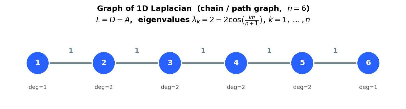Graph of the 1D Laplacian: a chain of n nodes 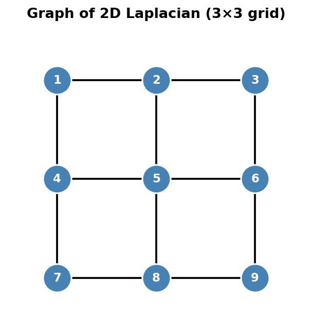Graph of the 2D Laplacian: a 3×3 grid of 9 nodes

7.2 Fill-in During Factorization

Recall that factorization can destroy the nice sparsity of a matrix. The graph perspective reveals precisely when fill-in occurs. Consider the LU factorization of a matrix \( A \) and focus on the first elimination step: one adds multiples of row 1 to rows \( 2, 3, \ldots, n \) to zero out the entries in the first column. While introducing those zeros, new non-zeros may appear in positions that were previously zero — this is fill-in.

From the graph perspective, eliminating node \( i \) transforms the graph according to two rules: (1) node \( i \) and all its edges are deleted, and (2) new edges \( j \leftrightarrow k \) are added for every pair of nodes \( j, k \) that were both connected to node \( i \) in the original graph but were not already connected to each other. These new edges correspond exactly to the fill-in entries. In other words, eliminating node \( i \) “cliques up” its neighborhood: all neighbors of \( i \) become connected to each other.

The same fill-in pattern arises for Cholesky factorization. At the first step of Cholesky, one computes the Schur complement \( B - vv^T/\alpha \). If a pair of rows in \( v \) are both non-zero (i.e., both rows connect to node 1 in the graph), then the corresponding entry in \( B - vv^T/\alpha \) becomes non-zero — exactly the same fill-in as in LU factorization, because both methods delete the same node and connect its neighbors.

A dramatic illustration is the arrow matrix, which has a dense first row and column plus diagonal entries. Every off-diagonal node is connected to node 1 but not to any other off-diagonal node. When node 1 is eliminated, all other nodes become connected to each other (since they all share node 1 as a neighbor), producing a completely dense lower-right block. By contrast, if the arrow is reversed (the dense row and column are last rather than first), then the hub node is eliminated last, and no fill-in occurs at all because none of the other nodes need to be connected before the hub is removed.

Fill-in comparison: natural ordering (dense fill) vs. hub-first ordering (no fill) for an arrow matrix

---

Matrix Reordering

Lectures 5 and 7 showed that general sparse matrices may have dense LU factors due to fill-in. The canonical example is the arrow matrix, whose LU factorization fills in the entire lower-right triangular block. This lecture introduces matrix reorderings — strategies for renumbering the nodes of the graph in order to produce LU factors with little or no fill-in.

8.1 Matrix Reordering — Key Idea

The graph structure of a matrix expresses the underlying relationships among variables. Crucially, the ordering (numbering) of the nodes and variables impacts the layout of the matrix but does not change the underlying graph or the solution. Different matrices with the same graph can suffer vastly different amounts of fill-in during factorization, depending solely on how the nodes are numbered. The goal of matrix reordering is therefore to renumber the graph nodes to produce a matrix whose factorization minimizes fill-in.

Mathematically, reordering is expressed using permutation matrices: a permutation matrix is the identity matrix \( I \) with some rows (or columns) swapped. Permuting the rows of \( A \) is equivalent to multiplying on the left by a permutation matrix \( P \), giving \( PA \). Permuting the columns is equivalent to multiplying on the right by a permutation matrix \( Q \), giving \( AQ \). Both can be applied simultaneously to give \( PAQ \). In practice, permutation matrices are never stored or multiplied explicitly; implementations use index arrays instead.

If one permutes \( A \) to \( \tilde{A} = PAQ \), then to solve the original system \( Ax = b \) one must reorder entries of both \( x \) and \( b \) to match the changes to \( A \). The permuted system is

\[ PAQ(Q^T x) = Pb, \quad \text{i.e.,} \quad \tilde{A}\tilde{x} = \tilde{b}, \]

where \( \tilde{x} = Q^T x \) and \( \tilde{b} = Pb \). After solving the permuted system for \( \tilde{x} \), the original solution is recovered by \( x = Q\tilde{x} \) (unpermuting).

Symmetric permutation is particularly important. A symmetric permutation replaces \( A \) with \( PAP^T \), permuting rows and columns in the same way (\( Q = P^T \). This is equivalent in graph terms to simply relabeling the nodes while leaving the edges unchanged, and it naturally preserves symmetry. To construct \( P \) from a reordering (a list of before-and-after node labels), one applies the desired row swaps to the identity matrix \( I \). For example, a reordering \( 1 \to 2,\; 2 \to 3,\; 3 \to 1,\; 4 \to 4 \) sends row 1 to row 2, row 2 to row 3, and row 3 to row 1, producing the permutation matrix with those row swaps applied to \( I \).

8.2 Example with Natural Ordering

As a concrete illustration, consider the 2D Laplacian matrix on a non-square domain with \( m_x \gg m_y \) (many more gridpoints in the \( x \)-direction than in the \( y \)-direction). With natural rowwise ordering (numbering along \( x \) first, then \( y \), the entries in row \( i \) of the matrix appear in columns \( i \) (diagonal), \( i-1 \) and \( i+1 \) (inner bands), and \( i-m_x \) and \( i+m_x \) (outer bands). Hence the bandwidth is \( m_x \).

By contrast, columnwise ordering (numbering along \( y \) first, then \( x \) produces outer bands of width \( m_y \), so the bandwidth is \( m_y \). Since \( m_x \gg m_y \), the columnwise ordering gives a much narrower bandwidth and therefore much less fill-in.

For banded matrix factorization, the bands of \( L \) and \( U \) have the same widths as the corresponding bands of \( A \). Fill-in can only occur in the region between the outermost bands. Recalling that banded Gaussian elimination costs approximately \( O(npq) \) flops for bandwidths \( p \) and \( q \), the total cost for bandwidth \( m \) is \( O(m^2 n) \). Rowwise ordering gives \( O(m_x^2 n) \) flops, while columnwise ordering gives only \( O(m_y^2 n) \) flops — a significant saving when \( m_x \gg m_y \).

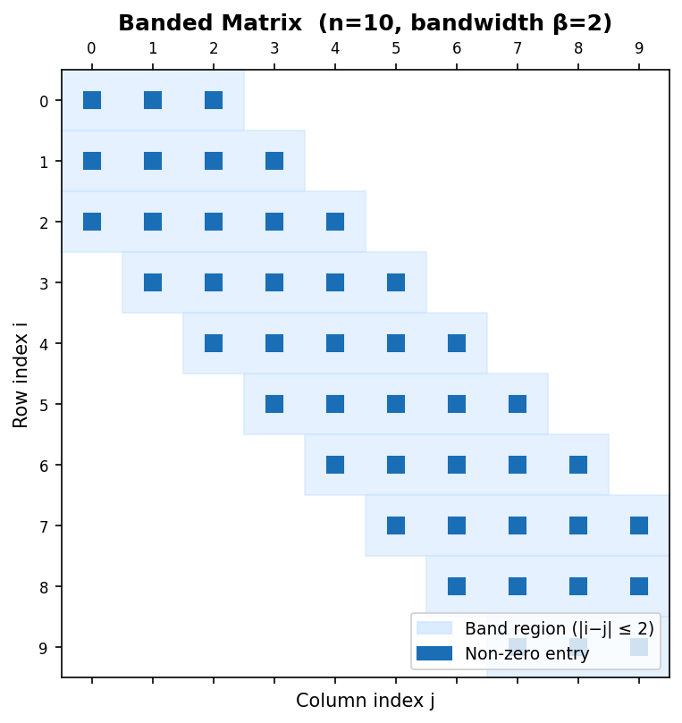Banded matrix (n=10, bandwidth β=2) with shaded band region

For more general sparsity patterns, finding the truly optimal ordering is an NP-complete problem. There exist many practical ordering algorithms based on good heuristics, including envelope/level set methods, (Reverse) Cuthill-McKee, Markowitz ordering, and minimum degree ordering. These algorithms are examined in subsequent lectures.

Worked Example: Graph Laplacian

This example illustrates computing the graph Laplacian for a weighted undirected graph and connecting it to the definitions of degree, weighted adjacency, indicator vectors, and set volumes.

The non-symmetric graph Laplacian is defined as \( L = D - W \), where \( D \) is the degree matrix and \( W \) is the weighted adjacency matrix. The degree matrix \( D \) is diagonal with the degree of each node on the diagonal; for a weighted graph the degree of node \( i \) is the sum of the weights of all edges incident to it.

For a specific six-node graph with nodes \( v_1, \ldots, v_6 \), computing the degrees: \( v_1 \) connects to \( v_2 \), \( v_3 \), and \( v_4 \) with weights 1, 1, and 2, giving degree \( 1 + 1 + 2 = 4 \). Node \( v_2 \) connects to \( v_1 \) and \( v_4 \) with weights 1 and 3, giving degree \( 1 + 3 = 4 \). Node \( v_3 \) connects to \( v_1 \), \( v_4 \), and \( v_6 \) with weights 1, 4, and 2, giving degree \( 1 + 4 + 2 = 7 \). Node \( v_4 \) connects to \( v_1 \), \( v_2 \), \( v_3 \), and \( v_5 \) with weights 2, 3, 4, and 2, giving degree \( 2 + 3 + 4 + 2 = 11 \). Node \( v_5 \) connects only to \( v_4 \) with weight 2, giving degree 2. Node \( v_6 \) connects only to \( v_3 \) with weight 2, giving degree 2.

The weighted adjacency matrix \( W \) has one row per vertex, with the edge weight \( w_{ij} \) in position \( (i,j) \) when nodes \( i \) and \( j \) share an edge. Because the graph is undirected, \( W \) is symmetric. The row sum for each node equals its degree, which can be seen directly from the structure of \( W \). The Laplacian \( L = D - W \) then has entries

\[ L = \begin{pmatrix} 4 & -1 & -1 & -2 & 0 & 0 \\ -1 & 4 & 0 & -3 & 0 & 0 \\ -1 & 0 & 7 & -4 & 0 & -2 \\ -2 & -3 & -4 & 11 & -2 & 0 \\ 0 & 0 & 0 & -2 & 2 & 0 \\ 0 & 0 & -2 & 0 & 0 & 2 \end{pmatrix}. \]

This graph Laplacian shares a key structural property with the finite difference discrete Laplacian: the diagonal entries are all positive, the off-diagonal entries are all non-positive, and each row sums to zero. For example, the first row: \( 4 - 1 - 1 - 2 = 0 \); in the finite difference stencil the analogous property was that the center coefficient 4 plus the four \( -1 \) neighbors sum to zero.

Finally, one can illustrate the definitions of indicator vectors, set volumes, and cut weights. Partition the six nodes into two subsets: \( A = \{v_1, v_2, v_6\} \) and \( B = \{v_3, v_4, v_5\} \). The indicator vector \( \mathbf{1}_A = [1, 1, 0, 0, 0, 1]^T \) has a 1 in position \( i \) if \( v_i \in A \) and 0 otherwise; similarly \( \mathbf{1}_B = [0, 0, 1, 1, 1, 0]^T \).

The cut weight \( W(A, B) \) is the sum of edge weights between the two sets: \( W(A,B) = \sum_{i \in A, j \in B} w_{ij} \). Enumerating all pairs: \( w_{13} + w_{14} + w_{15} + w_{23} + w_{24} + w_{25} + w_{63} + w_{64} + w_{65} \). Many of these are zero (no edge between the corresponding nodes): \( w_{15} = 0 \) (no edge between \( v_1 \) and \( v_5 \), \( w_{23} = 0 \), \( w_{25} = 0 \), \( w_{64} = 0 \), \( w_{65} = 0 \). The non-zero contributions are \( w_{13} = 1,\; w_{14} = 2,\; w_{24} = 3,\; w_{63} = 2 \), giving \( W(A,B) = 1 + 2 + 0 + 0 + 3 + 0 + 2 + 0 + 0 = 8 \).

The size of a set is just the number of vertices: \( |A| = 3 \) and \( |B| = 3 \). The volume of a set is the sum of degrees of its vertices: \( \text{vol}(A) = d_1 + d_2 + d_6 = 4 + 4 + 2 = 10 \) and \( \text{vol}(B) = d_3 + d_4 + d_5 = 7 + 11 + 2 = 20 \). These quantities — cut weight, size, and volume — are fundamental to spectral clustering and graph partitioning algorithms studied later in the course.

Envelope Reordering

Recall that finding the optimal reordering for a sparse matrix is NP-complete. In practice, reordering algorithms rely on good heuristics rather than an exhaustive search. This course covers four broad families of reordering methods: envelope and level-set methods, (Reverse) Cuthill-McKee, Markowitz, and Minimum Degree. The first two families are the subject of this lecture; the remaining two are treated in Lecture 10.

A central motivating observation is that, in practice, bandwidth may vary substantially between individual rows of a matrix. The envelope of a matrix is the smallest region around the diagonal where fill-in may occur. Because fill is confined to the envelope, a smaller envelope means less work during Gaussian elimination. The strategy is therefore to keep the envelope close to the diagonal, which translates into a graph-theoretic requirement: neighbouring nodes in the sparsity graph should receive numbers that are as close together as possible.

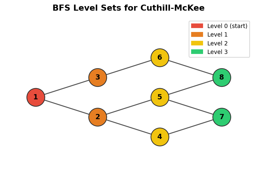BFS level sets on a graph, used as the basis for the Cuthill-McKee algorithm

9.1 Level Sets

We assume throughout that the sparsity pattern of the matrix is symmetric, so the underlying graph representation is undirected. Envelope methods are grounded in the notion of graph level sets.

Graph level sets \(S_i\) are groups of nodes that lie at the same graph distance from a chosen starting node. Formally, \(S_1\) consists of the single starting node; \(S_2\) contains all graph neighbours of nodes in \(S_1\); and in general \(S_i\) is the set of all graph neighbours of nodes in \(S_{i-1}\) that have not appeared in any earlier level set. Envelope methods then number nodes by processing each level set in turn: first all nodes in \(S_1\), then all in \(S_2\), and so on.

The level-set ordering algorithm is essentially a breadth-first search (BFS) of the graph. Starting from a chosen node \(s\), the algorithm marks \(s\) and places it in \(S_1\). At each subsequent step it expands the frontier: for every unmarked node adjacent to any node in the current level set \(S_i\), that node is added to \(S_{i+1}\) and marked. The process continues until no new nodes can be reached. For disconnected graphs, the procedure is repeated on each connected component. Two open questions within this basic framework are: in what order should nodes within a level set be enumerated, and in what order should the neighbours of a node be visited?

9.2 Cuthill-McKee

The Cuthill-McKee (CM) algorithm provides a heuristic answer to the within-level-set ordering question by exploiting node degrees. The degree of a node \(v\), written \(\deg(v)\), is the number of adjacent nodes, equivalently the number of incident edges. The Cuthill-McKee heuristic is: when visiting a node during the BFS traversal, add its as-yet-unnumbered neighbours to the queue in increasing order of degree, breaking ties by some fixed rule such as alphabetical order or original node index.

Concretely, the CM algorithm begins by picking a starting node and assigning it number 1. All unnumbered neighbours of node 1 are then numbered in increasing degree order. For each of those neighbours, their own unnumbered neighbours are in turn ordered by degree and queued, and the process continues until every node has received a number.

9.3 Reverse Cuthill-McKee

The Reverse Cuthill-McKee (RCM) algorithm is exactly what its name implies: compute the CM numbering, then reverse it. If there are \(n\) nodes, the RCM number of node \(i\) under CM becomes node \(n - i + 1\) under RCM. Although this reversal appears trivial, J. A. George observed in 1971 that it can substantially reduce the amount of fill-in for many graphs. RCM produces the same envelope bandwidth as CM, but the resulting sparsity patterns tend to resemble a lower-triangular “downward arrow” matrix rather than an upper-triangular “upward arrow” matrix, which is preferable for fill-reduction in practice.

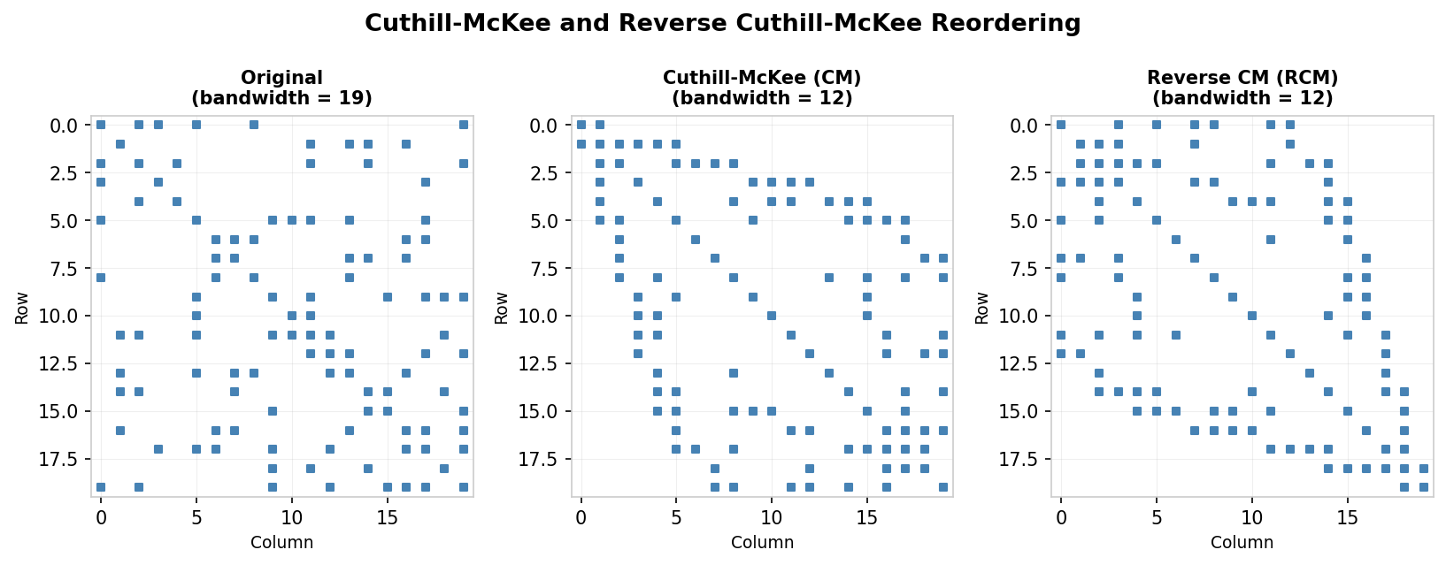Effect of CM and RCM reordering on bandwidth of a sparse symmetric matrix

A concrete illustration applies the CM algorithm starting from node B in a small graph, breaking ties alphabetically. The CM ordering gives a matrix whose entries cluster near the diagonal, but the RCM reversal of that numbering produces an ordering with even less fill. In the example shown in the lecture notes, the original matrix has 30 positions within its envelope where fill can occur, CM reduces this to 20, and RCM further reduces it to 12.

CM/RCM reordering on an arrow matrix reduces fill-in dramatically

The optimality of RCM on trees is a provable fact.

Theorem 9.1 (RCM is optimal on trees). On any tree, regardless of which starting node is chosen, the RCM ordering produces no fill during factorization.

The proof proceeds by showing that the first node in the RCM ordering must be a leaf (degree-1 node). Suppose for contradiction that the first node under RCM is a non-leaf \(u\), so \(u\) is connected to at least two nodes \(v\) and \(w\). Since the graph is a tree it contains no cycles, so the BFS from a starting node \(s\) can reach at most one of \(v, w\) before reaching \(u\). After reaching \(u\), the BFS must continue to the other child, so \(u\) cannot be the last node in the CM ordering, contradicting the assumption that its reversal is first in RCM. It follows that \(u\) must be a leaf. Removing the leaf \(u\) and rerunning CM on the remaining tree produces the same ordering (minus \(u\). Recursively, elimination always removes leaf nodes, never introducing new edges and hence never producing fill.

It is important to note that Theorem 9.1 does not extend to the plain CM ordering, and that RCM does not guarantee the globally optimal fill-reduction for general graphs. Determining the optimal ordering that minimises total fill-in is NP-complete [Yannakakis, 1981].

Worked Example: Cuthill-McKee and Reverse Cuthill-McKee

Consider a graph with nodes labelled A through J, and suppose we begin the Cuthill-McKee algorithm from node G, breaking ties alphabetically. The neighbours of G are H, E, B, and F. Their degrees are: H has degree 2, E has degree 3, and both B and F have degree 4. Within the level set of G, nodes are ordered by increasing degree, so the numbering proceeds: G receives 1, H receives 2, E receives 3, B receives 4, and F receives 5 (ties between B and F broken alphabetically).

We now expand from these four nodes. H’s neighbours are F and G, but both are already numbered, so H contributes nothing new. E’s neighbours include B (already numbered), G (already numbered), and C — so C is discovered here with degree 3, and receives number 6. B’s neighbours include C, E, G (all already numbered), and J, which has degree 1 and receives number 7. F’s neighbours include A (degree 2), D (degree 4), G, and H (both already numbered). Ordering A and D by increasing degree gives A number 8 and D number 9. Finally, D’s only unnumbered neighbour is I, which has degree 1 and receives number 10.

The complete CM ordering is therefore: G=1, H=2, E=3, B=4, F=5, C=6, J=7, A=8, D=9, I=10. Applying the reversal formula, the RCM ordering maps CM position \(i\) to RCM position \(n - i + 1\), so position 1 (G) becomes position 10, position 2 (H) becomes position 9, and so on.

In the original unnumbered matrix the envelope contains 30 positions where fill can occur. After applying CM this reduces to 20, and after applying RCM it reduces further to 12, illustrating the practical advantage of the reversal step.

---

Local Reorderings

The previous lecture established that the graph associated with a symmetric sparse matrix provides a powerful abstraction for understanding fill-in during factorization, and that envelope methods such as Reverse Cuthill-McKee can reduce fill by minimising the bandwidth. This lecture examines two complementary local strategies: Markowitz reordering and Minimum Degree reordering.

10.1 Markowitz Reordering

Markowitz reordering [Markowitz, 1957] is a local rule that greedily minimises fill-in for the current elimination step only, without attempting to optimise globally. After \(k\) steps of LU factorisation the matrix has been partially reduced to a remaining lower-right block \(A^{(k)}\). During one more step of LU, multiples of the pivot row are subtracted from rows below it, but only in columns where those rows have a nonzero entry. Fill-in does not occur in rows that already have a zero in the column to be eliminated.

For any candidate pivot entry \(a^{(k)}_{ij}\), let \(r^{(k)}_i\) denote the number of nonzeros in row \(i\) of \(A^{(k)}\) and \(c^{(k)}_j\) denote the number of nonzeros in column \(j\). The maximum possible fill-in introduced by using \(a^{(k)}_{ij}\) as the pivot is \((r^{(k)}_i - 1)(c^{(k)}_j - 1)\), which is called the Markowitz product. The Markowitz algorithm selects the pivot \(a^{(k)}_{pq}\) that minimises this product:

\[ (p, q) = \arg\min_{k \leq i,j} (r^{(k)}_i - 1)(c^{(k)}_j - 1). \]

The minimising entry is then swapped into the pivot position by permuting rows and columns. This is only an approximation of the true fill, since some of the positions that could in principle be filled may already be nonzero before the step begins.

For symmetric matrices, since \(\arg\min_i r^{(k)}_i = \arg\min_j c^{(k)}_j\), it suffices to examine only diagonal entries \(a^{(k)}_{pp}\) and to select

\[ p = \arg\min_{k \leq i} (r^{(k)}_i - 1). \]

Applying both a row and column swap symmetrically brings \(a^{(k)}_{pp}\) into the pivot position without breaking the symmetry of the matrix. This approach preserves diagonal dominance, which is important for stability, and corresponds directly to a node reordering in the graph representation.

10.2 Minimum Degree Reordering

The symmetric specialisation of Markowitz reordering leads naturally to the minimum degree algorithm. The quantity \(r^{(k)}_i - 1\) for a diagonal entry counts the number of off-diagonal nonzeros in row \(i\), which is precisely the degree of node \(i\) in the graph of \(A^{(k)}\). Minimising the Markowitz product for symmetric matrices is therefore equivalent to choosing the node with the smallest current degree as the next pivot.

Crucially, this graph-view decision can be computed before factorisation begins by renumbering nodes based on the elimination graph. Each step of Cholesky factorisation corresponds in the graph to: deleting the chosen node and all its edges, then connecting all its former neighbours together with new edges (those new edges represent fill). The minimum degree algorithm constructs this elimination graph iteratively, and at each step selects the node with the least current degree, removes it, adds the necessary fill edges, and relabels the graph.

When multiple nodes share the same minimum degree, tie-breaking strategies are needed. Common approaches include selecting the node with the smallest original index, pre-ordering with RCM and honouring that sequence, or using “multiple minimum degree” which simultaneously eliminates several non-interacting nodes of the same degree.

Comparison of minimum-degree reordering versus RCM

Minimum degree reordering is optimal on trees, because every elimination step in a tree removes a leaf node (degree 1) and never introduces new edges. However, it is still a local, greedy heuristic with no guarantee of global optimality for general graphs. A counterexample exists: consider a graph whose matrix envelope is already completely filled in. Factorisation can produce no additional fill. Yet minimum degree reordering would eliminate a low-degree interior node first, immediately introducing fill edges between its neighbours, degrading the structure.

Several improvements have been proposed to extend basic minimum degree. Supervariables (indistinguishable nodes) are groups of nodes with identical adjacency structure that can be eliminated simultaneously, reducing both computation and storage. Multiple elimination allows non-adjacent nodes of the same degree to be eliminated together safely. Approximate minimum degree (AMD) replaces exact degree updates with cheaper approximations, substantially reducing running time. A quotient graph representation provides a smarter data structure for tracking the evolving graph. In practice, Matlab’s symamd (symmetric approximate minimum degree) uses these ideas and often outperforms RCM, though it still provides no global optimality guarantee.

---

Stability of Factorizations

The story of this course up to this point has been: direct methods for solving linear systems rely on matrix factorisation; matrices often possess exploitable structure (sparsity, bandedness, symmetry, positive definiteness); reordering can reduce factorisation cost by limiting fill. This lecture turns to a different question — not how efficient the factorisation is, but how numerically reliable it is. A new use for row and column swaps emerges: not to reduce fill-in but to improve stability.

11.1 Conditioning versus Stability

How do small errors or perturbations to the matrix problem \(Ax = b\) affect the exact solution? The matrix condition number \(\kappa(A) = \|A\| \cdot \|A^{-1}\|\) provides a measure of this sensitivity, and satisfies \(\kappa \geq 1\). If the relative perturbations in \(A\) and \(b\) are both bounded by \(\delta\), then the relative change in the solution satisfies

\[ \frac{\|\Delta x\|}{\|x\|} \leq 2\kappa(A)\delta + O(\delta^2). \]

Stability is a distinct property from conditioning. Conditioning describes the intrinsic sensitivity of the mathematical problem; stability describes how errors introduced during computation (such as rounding) propagate through the numerical algorithm. A highly stable algorithm cannot rescue a poorly conditioned problem, but an unstable algorithm can produce meaningless results even when the underlying problem is well-conditioned. For LU factorisation, the basic goal is to keep the magnitudes of entries in \(L\) and \(U\) under control — huge entries inflate rounding errors and may render the product \(LU\) far from the original \(A\).

11.2 Pivoting

Factorisation as described so far assumes that each diagonal entry encountered as a pivot, \(a^{(k-1)}_{kk}\), is nonzero at each step. Problems arise when a pivot is exactly zero (division by zero) or close to zero (large round-off amplification). Pivoting addresses these problems by permuting rows or columns to bring a larger-magnitude entry into the pivot position before each elimination step.

Complete pivoting searches the entire remaining submatrix \(A^{(k-1)}\) for the entry of largest magnitude and swaps both its row and its column to the pivot position. Partial pivoting is less expensive: it searches only within the current column for the largest-magnitude entry and swaps only rows, placing that entry into the pivot position. For most practical problems, partial pivoting is sufficient.

LU factorisation with partial pivoting satisfies

\[ \hat{L}\hat{U} = \hat{P}A + \Delta A, \qquad \frac{\|\Delta A\|}{\|A\|} = O(\rho \epsilon_{\text{machine}}), \]

where \(\hat{P}\) is the computed permutation and \(\rho\) is the growth factor, approximately \(\rho \approx \|U\| / \|A\|\).

Partial pivoting can in principle fail: there exist contrived matrices for which successive elimination steps produce exponential growth in the entries of \(U\). In one classic family of examples the growth factor reaches \(\rho \approx 2^{n-1}\), causing \(\|U\|\) to dwarf \(\|A\|\). However, as Trefethen and Bau observe, “In fifty years of computing, no matrix problems that excite an explosive instability are known to have arisen under natural circumstances.” The cost of complete pivoting is therefore rarely justified, and partial pivoting yielding the factorisation \(PA = LU\) is standard practice.

There is also an important interaction between pivoting for stability and pivoting for sparsity: permuting for large pivots tends to destroy the sparsity pattern that reordering was designed to exploit. This trade-off must be managed carefully.

11.3 When Pivoting Is Unnecessary

For certain structured matrices, pivoting for stability is never required because the pivots are automatically positive throughout the factorisation.

Theorem 11.1. If \(A\) is symmetric positive definite (SPD), then during LU factorisation the pivot \(a^{(k-1)}_{kk} > 0\) for all \(k\).

The proof proceeds by induction on the matrix size. For a \(1 \times 1\) SPD matrix the single entry is a positive scalar. For \(n > 1\), write

\[ A = \begin{pmatrix} a_{11} & v^T \\ v & A_{22} \end{pmatrix}. \]

Since \(A\) is SPD its leading principal submatrices are positive definite, so \(a_{11} > 0\). One step of LU using \(a_{11}\) as the pivot transforms \(A\) to a new Schur complement

\[ A^{(1)}_{22} = A_{22} - \frac{vv^T}{a_{11}}. \]

One shows that \(A^{(1)}_{22}\) is itself SPD by constructing, for any nonzero \(x \in \mathbb{R}^{n-1}\), the vector \(y = (-x^T v / a_{11},\; x^T)^T \in \mathbb{R}^n\) and exploiting \(y^T A y > 0\). Repeating inductively, every subsequent pivot is positive.

Pivoting is also unnecessary for row diagonally dominant matrices, where \(|a_{kk}| > \sum_{j \neq k} |a_{kj}|\) for every row \(k\), and for column diagonally dominant matrices, where the analogous condition holds for each column. In both cases, the diagonal entry is guaranteed to dominate, ensuring well-conditioned pivots throughout.

---

Image Denoising

Digital images often contain random noise — small random errors — arising from sensors, capture conditions, or the stochastic nature of the measurement process. Synthetic images produced by ray-tracing also accumulate noise unless the simulation is run for an extremely long time; a practical alternative is to ray-trace briefly and then apply a mathematical denoising procedure to the result. The goal of image denoising is to recover, from a corrupted observation, a version of the image with the noise removed or substantially reduced.

12.1 Inverse Problems

Image denoising is an inverse problem: given observations, reconstruct the underlying source that generated them. Let \(u_0\) be the noisy observed image, \(u^*\) the unknown clean signal, and \(n\) the noise, so that \(u_0 = u^* + n\). We treat grayscale images as 2D scalar functions by writing \(u_{ij}\) for the pixel intensity at row \(i\), column \(j\). An estimate of the noise variance \(\|n\|_2^2 = \sigma^2\) is assumed known.

Two key assumptions make the inverse problem tractable: first, the noise is not too large, meaning the observation \(u_0\) is close to the true signal \(u^*\); second, the true signal has exploitable structure, typically smoothness. A PDE-based approach formulates the problem as an optimisation:

\[ \min_u \; \text{"fluctuation of pixel value"} \quad \text{subject to} \quad \|u - u_0\|_2^2 \approx \sigma^2. \]

The objective seeks to minimise rapid changes in pixel colour (assumed to be noise), while the constraint ensures the deviation of the solution from the observation matches the expected noise level. Because infinitely many decompositions of \(u_0\) satisfy the constraint, the problem is ill-posed and a choice of regularisation is needed to single out a particular solution.

12.2 Regularisation Models

Rather than working with the constrained form, it is often more convenient to work with the penalised form

\[ \min_u \; \alpha R(u) + \|u - u_0\|_2^2, \]

where \(R(u)\) is the regularisation model and \(\alpha > 0\) is the regularisation constant. The term \(\|u - u_0\|_2^2\) measures the discrepancy (fidelity to the observed data), while \(\alpha R(u)\) imposes smoothness or structure. As \(\alpha \rightarrow 0\) the regularisation term is ignored and the solution approaches \(u_0\) itself; as \(\alpha \rightarrow \infty\) the fidelity term is suppressed and the solution approaches the minimiser of \(R(u)\) alone. Good denoising requires appropriate tuning of \(\alpha\).

Tikhonov Regularisation. The simplest choice sets \(R(u) = \|u\|_2^2\), penalising large pixel intensities. The minimisation becomes

\[ \min_u \; \alpha \|u\|_2^2 + \|u - u_0\|_2^2. \]

Setting the gradient to zero and solving gives the closed-form solution \(u = u_0 / (\alpha + 1)\). While \(\alpha\) correctly interpolates between \(u_0\) and zero, this is not useful in practice: the ideal “perfectly regular” image is not an image of all zeros.

Laplacian Regularisation. A better idea is to penalise rapid changes in pixel intensity rather than the pixel values themselves. The Laplacian regularisation sets \(R(u) = \|\nabla u\|_2^2\), which measures the total squared gradient. The optimisation problem

\[ \min_u \; \alpha \|\nabla u\|_2^2 + \|u - u_0\|_2^2 \]

leads, via the Euler-Lagrange equations, to the linear PDE

\[ -\alpha \Delta u + u = u_0, \]

where \(\Delta = \nabla \cdot \nabla\) is the Laplace operator. Applying the five-point finite difference stencil for \(\Delta\) at each pixel \((i,j)\) gives

\[ \frac{\alpha}{h^2}(4u_{ij} - u_{i-1,j} - u_{i+1,j} - u_{i,j-1} - u_{i,j+1}) + u_{ij} = u^0_{ij}, \]

which is a linear system of the form \((\alpha A + I)u = u_0\). For persistent noise the solve can be iterated as \((\alpha A + I)u^{k+1} = u^k\). The main drawback of Laplacian regularisation is that it treats all gradients as equally undesirable, causing edges to be blurred along with noise.

Total Variation Regularisation. To preserve sharp edges while still removing noise from flat regions, total variation (TV) regularisation replaces the squared gradient by the \(\ell^1\)-norm of the gradient:

\[ R(u) = \|\nabla u\|_1. \]

The corresponding PDE is

\[ -\alpha \nabla \cdot \left(\frac{\nabla u}{|\nabla u|}\right) + u = u_0. \]

The key feature is the factor \(1/|\nabla u|\) in the diffusion coefficient. Near image edges where the intensity gradient is large, \(1/|\nabla u_{ij}|\) is small and the first PDE term becomes negligible, leaving \(u \approx u_0\) — edges are preserved. In flat regions where intensity is roughly constant, \(1/|\nabla u_{ij}|\) is large and the equation reduces to strong diffusion \(-C \Delta u + u = u_0\) with a large constant \(C\), smoothing the region aggressively. Total variation regularisation therefore smooths more in flat regions and smooths less near edges.

Because the PDE contains the solution-dependent coefficient \(1/|\nabla u|\), the discretised system \(\alpha A(u) + u = u_0\) is nonlinear. A fixed point iteration resolves the nonlinearity by “freezing” the coefficients at the current iterate: given the current estimate \(u^k\), form the coefficient matrix \(A(u^k)\) and solve the linear system

\[ \alpha(A(u^k) + I)u^{k+1} = u_0 \]

for \(u^{k+1}\), then update \(A\) and repeat. Iteration terminates when \(\|u^{k+1} - u^k\| < \text{tol}\). In this particular application the fixed point iteration converges. Increasing \(\alpha\) for TV regularisation progressively smooths the image while still preserving edges, in contrast to Laplacian regularisation where increasing \(\alpha\) simply blurs the entire image uniformly.

---

Iterative Methods

The previous lecture concluded the course’s treatment of direct methods for linear systems. Direct methods factor the matrix \(A\) and then solve the system in a finite, predetermined sequence of steps. This lecture begins the study of iterative methods, which instead generate a sequence of increasingly accurate approximations to the solution, terminating only when some prescribed tolerance is satisfied.

Iterative methods offer several potential advantages over direct methods. For large, sparse, high-dimensional problems they may be significantly faster. Because no fill-in occurs, they also tend to require much less memory: rather than storing an entire factored form of \(A\), one typically needs only vectors of size \(n\) and the matrix itself. LU factorisation costs \(O(n^3)\) in the worst (dense) case; each iteration of a splitting method costs only \(O(\text{nnz}(A))\) multiplied by the number of iterations. For applications where only an approximate solution is needed, iterative methods also allow “quitting early” at a user-specified tolerance, whereas a direct method produces no output at all until the entire factorisation is complete. When a good reordering cannot significantly reduce fill, iterative methods become the preferred approach for large problems.

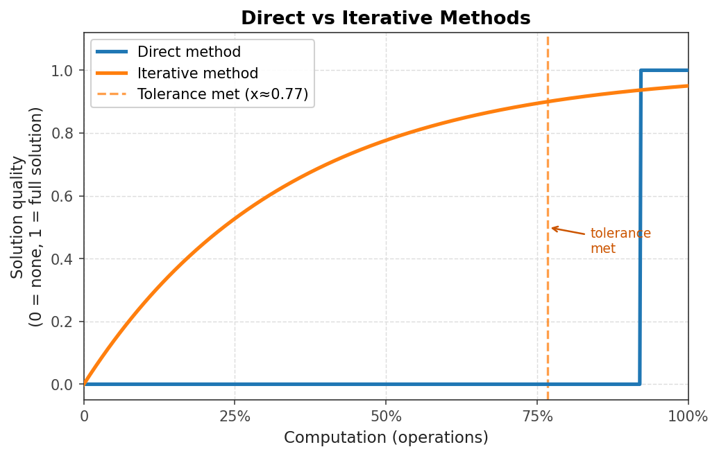Solution quality vs. computation: direct methods jump to full solution; iterative methods improve gradually

13.1 Termination Criterion

The error of an approximate solution \(\hat{x}\) is \(e = x - \hat{x}\), where \(x\) is the true solution. We terminate iteration when \(e \approx 0\). Since the true solution is unknown, a practical substitute is the residual \(r = b - A\hat{x}\), which measures how far the current approximation is from satisfying the linear system. The residual and error are related by \(Ae = r\), which follows from \(A(x - \hat{x}) = b - A\hat{x}\). The condition number then provides the bound

\[ \frac{\|e\|}{\|x\|} \leq \kappa(A) \frac{\|r\|}{\|b\|}. \]

A small residual implies a small error only when \(A\) is well-conditioned (small \(\kappa\).

13.2 Splitting Methods

The class of splitting methods reformulates \(Ax = b\) by writing \(A = M - N\), leading to the equivalent system \(Mx = Nx + b\). Starting from an initial guess \(x^0\), the iterative scheme is

\[ Mx^{k+1} = Nx^k + b, \]

which can be rearranged as

\[ x^{k+1} = x^k + M^{-1}(b - Ax^k) = x^k + M^{-1}r^k. \]

For this to be effective, \(M\) must be chosen so that (i) the linear system \(My = z\) is easy to solve, and (ii) \(M\) is a good approximation to \(A\). These two requirements are in tension: \(M = A\) converges in one step but requires solving the original system, while a very crude \(M\) is cheap to invert but may converge slowly.

Richardson Iteration. The simplest choice is \(M = \frac{1}{\theta}I\) for a chosen positive scalar \(\theta\), giving

\[ x^{k+1} = x^k + \theta(b - Ax^k). \]

Each component of \(x^{k+1}\) is a weighted combination of the old iterate and the residual. The cost per iteration is \(O(\text{nnz}(A))\) and two vectors must be stored.

Jacobi Iteration. A more informative splitting uses \(M = D\), the diagonal of \(A\). Denoting the strictly lower and upper triangular parts of \(-A\) as \(L\) and \(U\) respectively (so \(A = D - L - U\), the Jacobi iteration is

\[ x^{k+1} = x^k + D^{-1}(b - Ax^k). \]

Component-wise, this reads

\[ x^{k+1}_i = \frac{1}{a_{ii}}\left(b_i - \sum_{j \neq i} a_{ij} x^k_j\right). \]

Intuitively, each row equation is solved independently for its corresponding variable using all other variables at their current (step \(k\) values. The Jacobi iteration is trivially parallelisable: all components of \(x^{k+1}\) can be computed simultaneously from \(x^k\). Two vectors must be stored. However, Jacobi is generally slow to converge.

Gauss-Seidel Iteration. The Gauss-Seidel method differs from Jacobi in one crucial way: as soon as a component \(x^{k+1}_i\) is computed, it is immediately used in place of \(x^k_i\) for all subsequent components in the same sweep. That is,

\[ x^{k+1}_i = \frac{1}{a_{ii}}\left(b_i - \sum_{j < i} a_{ij} x^{k+1}_j - \sum_{j > i} a_{ij} x^k_j\right). \]

In matrix form this becomes \(M = D - L\), so

\[ (D - L)x^{k+1} = b + Ux^k \quad \Rightarrow \quad x^{k+1} = x^k + (D-L)^{-1}(b - Ax^k). \]

Gauss-Seidel typically converges faster than Jacobi and needs to store only a single vector (entries can be overwritten in-place). The trade-off is that Gauss-Seidel is inherently sequential and harder to parallelise. Red-black Gauss-Seidel addresses this by colouring the graph so that no two nodes of the same colour are neighbours, allowing all nodes of one colour to be updated simultaneously using only the (old) values of the other colour.

Backward Gauss-Seidel processes rows in reverse order (from \(i = n\) down to \(1\), swapping the roles of \(L\) and \(U\). Symmetric Gauss-Seidel combines one forward sweep with one backward sweep:

\[ x^{k+1/2} = x^k + (D-L)^{-1}(b - Ax^k), \quad x^{k+1} = x^{k+1/2} + (D-U)^{-1}(b - Ax^{k+1/2}). \]

Successive Over-Relaxation (SOR). A common acceleration strategy is to average the current iterate with the Gauss-Seidel update using a relaxation parameter \(\omega\):

\[ x^{k+1}_i = (1-\omega)x^k_i + \omega (x^{k+1}_i)_{\text{GS}}. \]

In matrix form the splitting matrix becomes \(M = \frac{1}{\omega}D - L\). For \(0 < \omega < 1\) this is called under-relaxation; for \(\omega > 1\) it is over-relaxation. For certain choices of \(\omega > 1\), SOR can converge substantially faster than plain Gauss-Seidel.

13.3 Convergence of Splitting Methods

The iteration can be written as

\[ x^{k+1} = (I - M^{-1}A)x^k + M^{-1}b. \]

The matrix \(I - M^{-1}A\) is called the iteration matrix. The key convergence questions are: under what conditions does the sequence converge, and how fast?

Definition. The spectral radius of a matrix \(B\) is \(\rho(B) = \max_i |\lambda_i|\), the largest eigenvalue magnitude.

Theorem 13.1. If \(\|I - M^{-1}A\| < 1\) for some induced matrix norm, then for any initial guess \(x^0\) the iteration converges to the true solution \(x^*\).

The proof subtracts the fixed-point equation \(x^* = (I - M^{-1}A)x^* + M^{-1}b\) from the iterative update to obtain \(x^{k+1} - x^* = (I - M^{-1}A)(x^k - x^*)\), yielding \(\|e^{k+1}\| \leq \|I - M^{-1}A\| \cdot \|e^k\|\). Since the norm factor is less than 1, the error shrinks monotonically.

Theorem 13.2. The iteration converges for any \(x^0\) and \(b\) if and only if \(\rho(I - M^{-1}A) < 1\).

The convergence factor \(\rho(I - M^{-1}A)\) controls the speed: smaller values (closer to 0) mean faster convergence, since the error satisfies \(\|x^{k+1} - x^*\| \leq \rho(I - M^{-1}A)\|x^k - x^*\|\).

Worked Example: Jacobi and Gauss-Seidel Iterations

Consider a \(2 \times 2\) linear system with coefficient matrix having diagonal entries \(a_{11} = 3\) and \(a_{22} = 3\), off-diagonal entries \(a_{12} = 2\) and \(a_{21} = 1\), and right-hand side \(b = (3, 1)^T\). The true solution is \(x^* = (1, 0)^T\). We start from the initial guess \(x^0 = (0, 0)^T\).

Jacobi, iteration \(k=1\). Each component is updated using only values from the previous iterate. For the first component: \(x^1_1 = 0 + \frac{1}{3}(3 - 2 \cdot 0) = 1\). For the second component: \(x^1_2 = 0 + \frac{1}{3}(1 - 1 \cdot 0) = \tfrac{1}{3}\). So after one Jacobi iteration, \(x^1 = (1, \tfrac{1}{3})^T\).

Jacobi, iteration \(k=2\). Using the values from \(x^1\): \(x^2_1 = \frac{1}{3}(3 - 2 \cdot \tfrac{1}{3}) = \tfrac{7}{9}\) and \(x^2_2 = \frac{1}{3}(1 - 1 \cdot 1) = 0\). So \(x^2 = (\tfrac{7}{9}, 0)^T\).

Jacobi, iteration \(k=3\). Continuing: \(x^3_1 = 1\) and \(x^3_2 \approx 0.074\). The iterates are converging toward \(x^* = (1, 0)^T\) but have not yet arrived.

Gauss-Seidel, iteration \(k=1\). The first component is updated identically to Jacobi: \(x^1_1 = \frac{1}{3}(3 - 2 \cdot 0) = 1\). However, for the second component we immediately use the freshly computed value \(x^1_1 = 1\) rather than the old value 0: \(x^1_2 = \frac{1}{3}(1 - 1 \cdot 1) = 0\). After just one Gauss-Seidel iteration, \(x^1 = (1, 0)^T = x^*\). Gauss-Seidel has converged to the exact solution in a single iteration, compared to the slow convergence of Jacobi. This illustrates the practical advantage of using the most recently computed values immediately.

---

Steepest Descent

Lecture 13 introduced stationary splitting methods for iteratively solving \(Ax = b\). This lecture develops a different approach grounded in optimisation. We assume throughout that \(A \in \mathbb{R}^{n \times n}\) is symmetric positive definite (SPD) and consider the quadratic function

\[ F(x) = \frac{1}{2}x^T A x - b^T x, \quad x \in \mathbb{R}^n. \]

Because \(A\) is SPD, \(F\) is strictly convex, and its graph in the case \(n = 2\) is a paraboloid with a unique minimum at \(x = A^{-1}b\).

Theorem 14.1. Solving \(Ax = b\) is equivalent to minimising \(F(x)\).

The gradient is \(\nabla F(x) = Ax - b\), so \(\nabla F(x) = 0\) if and only if \(Ax = b\). Since \(F\) is strictly convex, this stationary point is the global minimum.

The quadratic form F(x) = ½xᵀAx − xᵀb defines a paraboloid in n dimensions

14.1 Solution by Steepest Descent

To find the minimum we “walk downhill”. At each step we choose a nonzero search direction \(p\) and then determine the scalar step length \(\alpha\) that minimises \(F\) along that direction:

\[ x^{k+1} = x^k + \alpha p. \]

Substituting into \(F\) and differentiating with respect to \(\alpha\) gives the optimal step length

\[ \alpha = \frac{p^T r^k}{p^T A p}, \]

where \(r^k = b - Ax^k\) is the residual at the current iterate. Since \(A\) is SPD, \(p^T A p > 0\) is guaranteed, so \(\alpha\) is well-defined.

The optimal search direction at each step is the one that reduces \(F\) most rapidly. The rate of change of \(F\) along \(p\) at the current point is \(f'(0) = p^T \nabla F(x^k) = p^T(Ax^k - b)\). To minimise this over unit vectors \(p\), choose \(p = -\nabla F(x^k) / \|\nabla F(x^k)\|\). Since \(\nabla F(x^k) = Ax^k - b = -r^k\), the direction of steepest descent is \(p = r^k\) (normalisation is unnecessary). This gives the steepest descent iteration:

\[ x^{k+1} = x^k + \alpha_k r^k, \quad \alpha_k = \frac{(r^k)^T r^k}{(r^k)^T A r^k}. \]

The residual can be updated cheaply without recomputing \(Ax^{k+1}\) from scratch:

\[ r^{k+1} = r^k - \alpha_k A r^k, \]

reusing the matrix-vector product \(Ar^k\) already computed to find \(\alpha_k\).

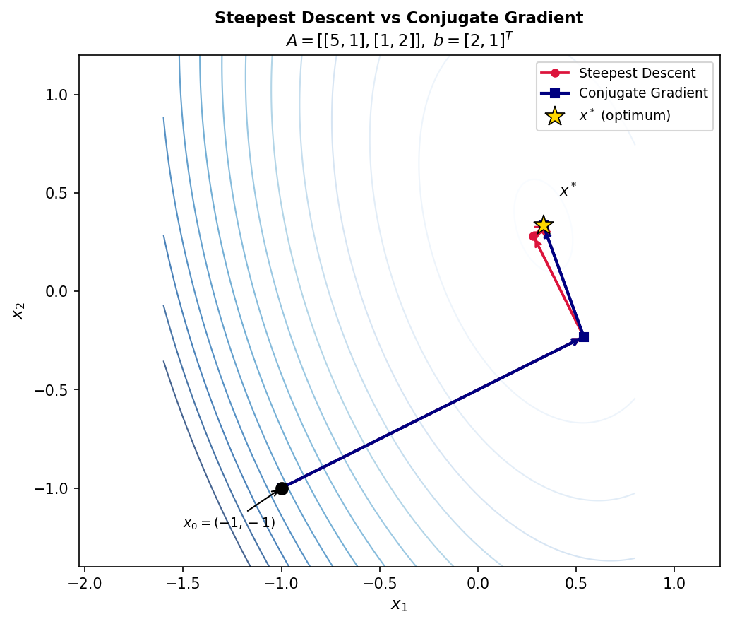Contours of F(x) with steepest descent and conjugate gradient paths

Despite being locally optimal at each step, the steepest descent method often converges slowly in practice, exhibiting a characteristic zig-zag path towards the solution. For an SPD matrix with eigenvalues satisfying \(\lambda_{\min} \leq \lambda \leq \lambda_{\max}\), the error in the A-norm (also called the energy norm, \(\|x\|_A = \sqrt{x^T Ax}\) satisfies the bound

\[ \|e^{k+1}\|_A \leq \frac{\lambda_{\max} - \lambda_{\min}}{\lambda_{\max} + \lambda_{\min}} \|e^k\|_A. \]

The convergence factor \((\lambda_{\max} - \lambda_{\min})/(\lambda_{\max} + \lambda_{\min})\) is close to 1 when the matrix is ill-conditioned (large condition number \(\lambda_{\max}/\lambda_{\min}\), leading to very slow convergence. This motivates the conjugate gradient method of the next lecture.

Worked Example: One Step of Steepest Descent

Consider the linear system with matrix \(A = \begin{pmatrix}3 & 2 \\ 2 & 6\end{pmatrix}\) and right-hand side \(b = (2, -8)^T\), with true solution \(x^* = (2, -2)^T\). We start from the initial guess \(x^0 = (-2, -2)^T\).

The initial residual is \(r^0 = b - Ax^0 = (2, -8)^T - \begin{pmatrix}3&2\\2&6\end{pmatrix}(-2,-2)^T\). Computing the matrix-vector product: \(A x^0 = (-10, -16)^T\), so \(r^0 = (2-(-10),\,-8-(-16))^T = (12, 8)^T\).

The step length is \(\alpha_0 = (r^0)^T r^0 / (r^0)^T A r^0\). The numerator is \(12^2 + 8^2 = 144 + 64 = 208\). For the denominator: \(Ar^0 = \begin{pmatrix}3&2\\2&6\end{pmatrix}(12,8)^T = (52, 72)^T\), so \((r^0)^T Ar^0 = 12 \cdot 52 + 8 \cdot 72 = 624 + 576 = 1200\). Hence \(\alpha_0 = 208/1200 \approx 0.1733\).

The updated solution is \(x^1 = x^0 + \alpha_0 r^0 = (-2,-2)^T + 0.1733 \cdot (12,8)^T \approx (0.0796, -0.6136)^T\). The true solution is \(x^* = (2,-2)^T\), so the first iterate is still quite far off.

Updating the residual: \(r^1 = r^0 - \alpha_0 A r^0 = (12,8)^T - 0.1733 \cdot (52,72)^T \approx (2.988, -4.478)^T\). The residual remains large in magnitude, illustrating the characteristic slow progress of steepest descent. Running the full algorithm would produce a zig-zag sequence of iterates spiralling in toward the true solution, a well-known pathology of the method that the conjugate gradient method is designed to overcome.

---

Conjugate Gradient Method

Steepest descent chooses the locally fastest downhill direction at every step, yet the resulting zig-zag path to the solution can be extremely slow. The root cause is that the locally optimal direction at step \(k\) may undo progress made at earlier steps. This lecture develops the conjugate gradient (CG) method, which selects search directions more globally and achieves exact convergence in at most \(n\) steps in exact arithmetic.

15.1 A-Orthogonality and Conjugate Directions

An ideal iteration would find the solution component by component along \(n\) independent directions, each searched exactly once. Choosing the coordinate axes as search directions does not work: the minimum of \(F\) along a coordinate axis is not the true solution restricted to that axis. A better notion of “independent directions” is needed.

Assuming \(A\) is SPD, the A-inner product is \((p,q)_A = p^T A q\) and the A-norm is \(\|p\|_A = \sqrt{(p,p)_A}\). Two vectors are A-orthogonal (or conjugate) if \((p,q)_A = 0\). A-orthogonality is a form of orthogonality that respects the geometry induced by \(A\): vectors that are A-orthogonal become ordinary orthogonal vectors after transforming to the coordinate system scaled by \(A\).

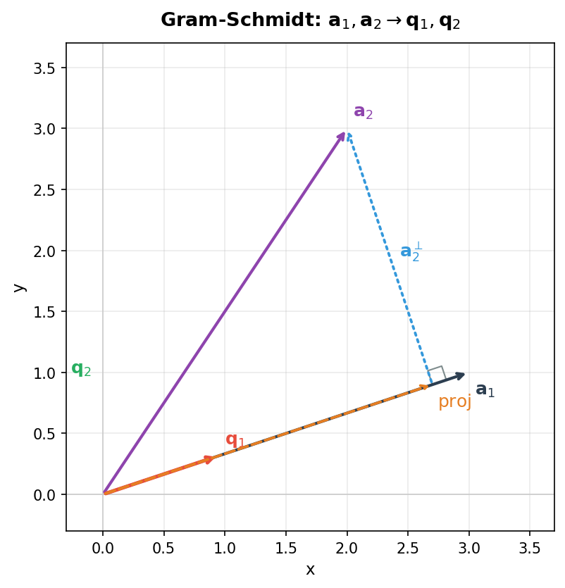A-orthogonal conjugate directions

The conjugate directions method constructs a set of mutually A-orthogonal search directions \(p^0, p^1, \ldots, p^{n-1}\) using Gram-Schmidt A-orthogonalisation. Given a proposed direction \(u^k\) and the prior search directions \(p^0, \ldots, p^{k-1}\) (mutually A-orthogonal), form

\[ p^k = u^k + \sum_{i=0}^{k-1} \beta_i p^i \]

with coefficients determined by A-orthogonality: requiring \((p^k, p^j)_A = 0\) for all \(j < k\) gives

\[ \beta_j = -\frac{(u^k, p^j)_A}{(p^j, p^j)_A}. \]

The same step length formula as steepest descent applies with the new directions: \(\alpha_k = (r^k)^T p^k / (p^k)^T A p^k\). The drawback of this approach as stated is that one must store all prior search vectors and perform a full Gram-Schmidt at each step, costing \(O(n^3)\) overall. The choice of input vectors \(u^k\) is also left open.

15.2 The Efficient Conjugate Gradient Algorithm

The conjugate gradient method resolves both difficulties by a single elegant choice: set \(u^k = r^k\), the current residual. This choice, combined with careful exploitation of orthogonality relationships, collapses the full Gram-Schmidt to a single-term recurrence.

The search directions and residuals generated by CG span the same spaces:

\[ \text{span}\{p^0, p^1, \ldots, p^{k-1}\} = \text{span}\{r^0, r^1, \ldots, r^{k-1}\} = \text{span}\{r^0, Ar^0, A^2r^0, \ldots, A^{k-1}r^0\} = \mathcal{K}_k(A, r^0). \]

This \(k\)-dimensional space is called the Krylov subspace \(\mathcal{K}_k(A, r^0)\). A key property is that \(r^k \perp \mathcal{K}_k(A, r^0)\), meaning the current residual is orthogonal to all prior residuals and search directions.

This orthogonality implies that the Gram-Schmidt sum collapses dramatically. In the formula \(p^k = r^k - \sum_{i=0}^{k-1} \frac{(r^k, p^i)_A}{(p^i, p^i)_A} p^i\), one can show that \((r^k, p^i)_A = 0\) for all \(i \leq k-2\). The argument proceeds through Krylov subspace inclusions: since \(p^i \in \text{span}\{p^0, \ldots, p^i\} = \text{span}\{r^0, Ar^0, \ldots, A^i r^0\}\), it follows that \(Ap^i \in \text{span}\{Ar^0, A^2 r^0, \ldots, A^{i+1} r^0\} \subseteq \text{span}\{r^0, r^1, \ldots, r^{i+1}\}\). But \(r^k \perp \text{span}\{r^0, \ldots, r^{i+1}\}\) whenever \(i + 1 \leq k - 1\), so \((r^k, p^i)_A = (r^k, Ap^i) = 0\) for all \(i \leq k - 2\). Thus only the \(i = k-1\) term survives:

\[ p^k = r^k + \beta_{k-1} p^{k-1}, \quad \beta_{k-1} = \frac{(r^k, r^k)}{(r^{k-1}, r^{k-1})}. \]

The simplified formula for \(\beta_{k-1}\) follows from a chain of algebraic identities. From the residual recurrence \(r^k = r^{k-1} - \alpha_{k-1} A p^{k-1}\), taking the inner product with \(r^k\) and using \((r^k, r^{k-1}) = 0\) gives \((r^k, Ap^{k-1}) = \frac{1}{\alpha_{k-1}}(r^k, r^k)\). Similarly, taking the inner product of the residual recurrence with \(p^{k-1}\) and using \((r^k, p^{k-1}) = 0\) yields \((p^{k-1}, Ap^{k-1}) = \frac{1}{\alpha_{k-1}}(r^{k-1}, r^{k-1})\). Dividing the two expressions produces \(\beta_{k-1} = (r^k, r^k)/(r^{k-1}, r^{k-1})\).

The step length simplifies similarly. Since \((r^k, p^k) = (r^k, r^k)\) by orthogonality, the step length becomes

\[ \alpha_k = \frac{(r^k, r^k)}{(p^k, p^k)_A}. \]

The resulting efficient algorithm is:

Algorithm (Conjugate Gradient, version 2.0).

• Initialise: \(x^0\) = initial guess, \(r^0 = b - Ax^0\), \(\beta_{-1} = 0\).
• For \(k = 0, 1, 2, \ldots, n-1\):
  • \(\beta_{k-1} = (r^k, r^k)/(r^{k-1}, r^{k-1})\)
  • \(p^k = r^k + \beta_{k-1} p^{k-1}\)
  • \(\alpha_k = (r^k, r^k) / (p^k, Ap^k)\)
  • \(x^{k+1} = x^k + \alpha_k p^k\)
  • \(r^{k+1} = r^k - \alpha_k Ap^k\)

Each iteration requires exactly one matrix-vector multiplication (\(Ap^k\) and two inner products (\((r^k, r^k)\) and \((p^k, Ap^k)\). Only the current vectors \(x^k, r^k, p^k\) and \(p^{k-1}\) need to be stored.

15.3 Error Behaviour and Convergence

Since the search directions \(p^0, \ldots, p^{n-1}\) are mutually A-orthogonal and span \(\mathbb{R}^n\), the algorithm terminates in at most \(n\) steps with the exact solution (in exact arithmetic). In fact, at each step CG eliminates exactly one component of the initial error. Expressing \(e^0 = x^0 - x^* = \sum_{j=0}^{n-1} \delta_j p^j\) and exploiting A-orthogonality shows \(\alpha_k = \delta_k\), so after \(k\) iterations

\[ e^k = \sum_{j=k}^{n-1} \delta_j p^j. \]

Equivalently, the CG iterate \(x^k\) minimises the A-norm of the error over the Krylov subspace \(\mathcal{K}_k(A, r^0)\):

\[ x^k = \arg\min_{x \in \mathcal{K}_k} \\|e^k\\|_A^2. \]

In practice, CG often converges in far fewer than \(n\) iterations, especially when the spectrum of \(A\) is clustered. This makes it substantially more effective than steepest descent, which exhibits zig-zag behaviour whenever the condition number is large.

Steepest descent (red, zigzag) vs. conjugate gradient (blue, direct) on elliptic contours

---

Least Squares Problems

All previous lectures have focused on square linear systems \(Ax = b\) where \(A \in \mathbb{R}^{n \times n}\). This lecture addresses the case where there are more equations than unknowns: \(A \in \mathbb{R}^{m \times n}\) with \(m \geq n\). Such systems are called over-determined because the constraints outnumber the degrees of freedom, and in general no exact solution exists. The goal is to find the \(x\) that satisfies the system “as well as possible”.

16.1 The Least Squares Formulation

Least squares problems were first posed by Gauss around 1795 (though published first by Legendre in 1805). They arise naturally in data fitting: given many observations, find a model with fewer parameters that best fits all the data. The mathematical formulation is

\[ \min_{x \in \mathbb{R}^n} \\|b - Ax\\|_2^2, \quad A \in \mathbb{R}^{m \times n},\; b \in \mathbb{R}^m,\; m \geq n. \]

Geometrically, the set of all vectors of the form \(Ax\) as \(x\) ranges over \mathbb{R}^n) forms a subspace of \mathbb{R}^m) called the range of \(A\). The least squares problem asks for the point in this range that is closest to \(b\), i.e., the projection of \(b\) onto the range of \(A\).

Theorem 16.1. Let \(A \in \mathbb{R}^{m \times n}\), \(b \in \mathbb{R}^m\), \(m \geq n\), and \(A\) full column rank. A vector \(x \in \mathbb{R}^n\) minimises \|b - Ax\|_2^2) if and only if \(r = b - Ax\) is orthogonal to the range of \(A\).

Theorem 16.1 implies that the minimiser satisfies \(A^T r = 0\), i.e., \(A^T(b - Ax) = 0\), which gives the normal equations:

\[ A^T A x = A^T b. \]

The normal equations form a square \(n \times n\) system. When \(A\) is full column rank, \(A^T A\) is symmetric positive definite and the system has a unique solution. This motivates the Moore-Penrose pseudoinverse:

\[ A^+ = (A^T A)^{-1} A^T, \]

so the least squares solution is \(x = A^+ b = (A^T A)^{-1} A^T b\). Any perturbation of \(x\) increases the residual norm: for \(x' = x + e\) with \(e \neq 0\), one can show \|b - Ax’|_2 > \|b - Ax\|_2) by expanding and using the normality condition \(A^T(b - Ax) = 0\).

16.2 Method 1: Normal Equations

The straightforward approach solves the normal equations \(A^T A x = A^T b\) directly. Since \(A^T A\) is SPD, the preferred factorisation is Cholesky: \(A^T A = GG^T\) with \(G\) lower triangular, followed by forward and backward solves. The dominant costs are forming \(A^T A\) (requiring approximately \(mn^2\) flops using symmetry) and computing the Cholesky factorisation (\(\frac{1}{3}n^3\) flops).

As a concrete application, consider polynomial fitting by least squares. Given \(m\) data points \({(t_i, y_i)}_{i=1}^m), we seek a degree-\((n-1)\) polynomial \(p(t) = a_0 + a_1 t + a_2 t^2 + \cdots + a_{n-1} t^{n-1}\) that best fits the data. Each data point generates one equation, so the full system is

\[ \begin{pmatrix} 1 & t_1 & t_1^2 & \cdots & t_1^{n-1} \\ 1 & t_2 & t_2^2 & \cdots & t_2^{n-1} \\ \vdots & \vdots & \vdots & \ddots & \vdots \\ 1 & t_m & t_m^2 & \cdots & t_m^{n-1} \end{pmatrix} \begin{pmatrix} a_0 \\ a_1 \\ \vdots \\ a_{n-1} \end{pmatrix} = \begin{pmatrix} y_1 \\ y_2 \\ \vdots \\ y_m \end{pmatrix}. \]

The coefficient matrix is called a Vandermonde matrix. As a concrete example, suppose the data points are \(\{(0,0),(0,-1),(2,1),(2,0),(4,2),(4,1)\}\) and we seek the best-fit line \(y = a_0 + a_1 t\). The matrix \(A\) is \(6 \times 2\) with columns of ones and of the \(t\)-values. Computing the normal equations gives

\[ A^T A = \begin{pmatrix} 6 & 12 \\ 12 & 40 \end{pmatrix}, \quad A^T b = \begin{pmatrix} 3 \\ 14 \end{pmatrix}. \]

Solving \(A^T A x = A^T b\) yields \(a_0 = -\tfrac{1}{2}\) and \(a_1 = \tfrac{1}{2}\), giving the least squares line \(y = -\tfrac{1}{2} + \tfrac{1}{2}t\). This is the unique line minimising the sum of squared vertical distances to the six data points.

The normal equations approach is straightforward to implement but can suffer from numerical issues: forming \(A^T A\) squares the condition number, so \(\kappa(A^T A) = \kappa(A)^2\). An alternative approach — QR factorisation — avoids this squaring and is discussed in the next lecture.

QR Factorization

Lecture 16 discussed the first method for solving least squares problems via the normal equations. This lecture discusses a second approach using QR factorization. The QR factorization decomposes a matrix \( A \) into an orthogonal matrix \( Q \) and a triangular matrix \( R \). Before developing this factorization, it is useful to review properties of orthogonal matrices, since these properties underpin the existence and usefulness of QR.

17.1 Orthogonal Matrices and Orthonormality

Definition 17.1. A square matrix \( Q \) is orthogonal if \( Q^{-1} = Q^T \), i.e., \( Q^T Q = Q Q^T = I \).

A key property of orthogonal matrices is that they preserve vector norms.

Theorem 17.1. If \( Q^T Q = I \), then \( \|Qx\|_2 = \|x\|_2 \).

The proof follows directly: \( \|Qx\|^2 = (Qx)^T(Qx) = x^T Q^T Q x = x^T x = \|x\|^2 \). Geometrically, multiplication by an orthogonal matrix corresponds to a rotation when \( \det(Q) = 1 \), and a reflection when \( \det(Q) = -1 \).

Definition 17.2. A set of vectors is orthonormal if they are mutually orthogonal and each vector has norm equal to 1.

An important distinction: orthogonal vectors need not have unit length, but the columns of an orthogonal matrix are always orthonormal. This terminology can be confusing and deserves careful attention.

The following theorem establishes the existence of the QR factorization.

Theorem 17.2. Suppose \( A \in \mathbb{R}^{m \times n} \) has full rank. Then there exists a unique matrix \( \hat{Q} \in \mathbb{R}^{m \times n} \) satisfying \( \hat{Q}^T \hat{Q} = I \) (i.e., with orthonormal columns) and a unique upper triangular matrix \( \hat{R} \in \mathbb{R}^{n \times n} \) with positive diagonals (\( r_{ii} > 0 \) such that \( A = \hat{Q}\hat{R} \).

Note that because \( \hat{Q} \) is non-square in general, it is not itself an orthogonal matrix in the strict sense of Definition 17.1.

17.2 QR for Least Squares

Consider the least squares problem \( \min_x \|Ax - b\|_2 \). We try to minimize this by re-expressing \( Ax - b \) in terms of the QR factorization. Since \( A = \hat{Q}\hat{R} \), we can write

\[ Ax - b = \hat{Q}\hat{R}x - b = \hat{Q}(\hat{R}x - \hat{Q}^T b) - (I - \hat{Q}\hat{Q}^T)b. \]

One can verify that the two vectors \( \hat{Q}(\hat{R}x - \hat{Q}^T b) \) and \( (I - \hat{Q}\hat{Q}^T)b \) are orthogonal to each other. By Pythagoras,

\[ \|Ax - b\|^2 = \|\hat{Q}(\hat{R}x - \hat{Q}^T b)\|^2 + \|(I - \hat{Q}\hat{Q}^T)b\|^2 = \|\hat{R}x - \hat{Q}^T b\|^2 + \|(I - \hat{Q}\hat{Q}^T)b\|^2. \]

The second equality uses the norm-preserving property of \( \hat{Q} \). The second term cannot be adjusted by choice of \( x \). The norm is therefore minimized by setting the first term to zero, yielding the least squares solution

\[ \hat{R}x = \hat{Q}^T b \quad \Rightarrow \quad x = \hat{R}^{-1}\hat{Q}^T b. \]

Orthogonal decomposition used in least squares: b = Ax + r where r ⊥ range(A)*

The pseudoinverse written in terms of QR factors is \( A^+ = \hat{R}^{-1}\hat{Q}^T \). One can also show that this solution is consistent with the normal equations: starting from \( A^T A x = A^T b \) and substituting \( A = \hat{Q}\hat{R} \) leads directly to \( \hat{R}x = \hat{Q}^T b \), confirming that all three formulations are equivalent.

17.3 Two Sizes of QR Factorization

The factorization \( A = \hat{Q}\hat{R} \) with \( \hat{Q} \in \mathbb{R}^{m \times n} \) and \( \hat{R} \in \mathbb{R}^{n \times n} \) is called the reduced (economy-size) QR factorization. The full QR factorization appends \( m - n \) additional orthonormal columns to \( \hat{Q} \) to make \( Q \) square (and thus a true orthogonal matrix), while adding corresponding zero rows to \( R \). Defining \( \hat{Q}_{m-n} = [q_{n+1} \; q_{n+2} \; \cdots \; q_m] \), the full factorization takes the block form

\[ A_{m \times n} = \begin{bmatrix} \hat{Q} & \hat{Q}_{m-n} \end{bmatrix}_{m \times m} \begin{bmatrix} \hat{R} \\ 0 \end{bmatrix}_{m \times n}. \]

The full QR is often useful for theoretical purposes. In practice the reduced version suffices for least squares computations.

17.4 Computing the Reduced QR Factorization

To compute the reduced QR factorization, let \( A = [a_1 \; a_2 \; \cdots \; a_n] \) where \( a_i \) are the columns of \( A \). We want to find a set of orthonormal column vectors \( \{q_i\} \) spanning the same column space, i.e.,

\[ \text{span}\{q_1, q_2, \ldots, q_j\} = \text{span}\{a_1, a_2, \ldots, a_j\}, \quad j = 1, \ldots, n. \]

This is accomplished by Gram-Schmidt orthogonalization, which builds each new vector \( q_j \) by orthogonalizing \( a_j \) against all previously constructed \( q \) vectors and then normalizing. The entries of \( R \) follow from comparing the Gram-Schmidt expressions to the column equations of the QR factorization. The next lecture develops this approach in detail.

---

Gram-Schmidt Orthogonalization

We have already encountered a variation of Gram-Schmidt orthogonalization when constructing \( A \)-orthogonal search directions for the conjugate gradient method. The same general idea applies here to construct the QR factorization: use the columns of \( A \) as proposed vectors to be orthogonalized into \( Q \), building each new vector \( q_j \) by orthogonalizing \( a_j \) against all previous \( q \) vectors and then normalizing.

18.1 QR Factorization via Gram-Schmidt

Orthonormalization for Q. For a vector \( a_j \), we orthogonalize it against all previous vectors \( q_i \) for \( i = 1, \ldots, j-1 \) using

\[ v_j = a_j - (q_1^T a_j)q_1 - (q_2^T a_j)q_2 - \cdots - (q_{j-1}^T a_j)q_{j-1}. \]

This removes \( a_j \)’s components in the previously constructed orthogonal directions. We then normalize to obtain

\[ q_j = \frac{v_j}{\|v_j\|}. \]

The derivation of this formula follows by assuming \( v_j = a_j + \sum_{i=1}^{j-1} \beta_i q_i \) and imposing the orthogonality condition \( q_k^T v_j = 0 \) for each \( k = 1, \ldots, j-1 \). Since \( q_k^T q_k = 1 \) and \( q_k^T q_i = 0 \) for \( i \neq k \), one obtains \( \beta_k = -q_k^T a_j \).

As a concrete illustration in 2D: given \( a_2 \) and the already-constructed unit vector \( q_1 \), we compute \( v_2 = a_2 - (q_1^T a_2)q_1 \) (orthogonalize) and then set \( q_2 = v_2 / \|v_2\| \) (normalize).

Gram-Schmidt process: a₁, a₂ → q₁, q₂

Upper Triangular Matrix R. To identify the entries of \( R \), expand the QR factorization column by column:

\[ a_1 = r_{11} q_1, \quad a_2 = r_{12} q_1 + r_{22} q_2, \quad a_3 = r_{13} q_1 + r_{23} q_2 + r_{33} q_3, \quad \ldots \]

Comparing with the Gram-Schmidt expressions gives the general formulas

\[ r_{ij} = q_i^T a_j, \quad r_{jj} = \left\| a_j - \sum_{i=1}^{j-1} r_{ij} q_i \right\|. \]

The off-diagonal entries \( r_{ij} \) are the lengths of the components of \( a_j \) in the directions \( q_1, \ldots, q_{j-1} \). The diagonal entries \( r_{jj} \) are the norms of the intermediate vectors \( v_j \), used to normalize into \( q_j \).

The Classic Gram-Schmidt algorithm (Algorithm 18.1) proceeds as follows. For each column \( j = 1, \ldots, n \), initialize \( v_j = a_j \), then for \( i = 1, \ldots, j-1 \) compute \( r_{ij} = q_i^T a_j \) and update \( v_j = v_j - r_{ij} q_i \). Finally set \( r_{jj} = \|v_j\|_2 \) and \( q_j = v_j / r_{jj} \). The classic Gram-Schmidt is numerically unstable: it is sensitive to round-off error and can yield vectors \( q_j \) that are no longer orthogonal.

18.2 Modified Gram-Schmidt

The Modified Gram-Schmidt algorithm (Algorithm 18.2) alters the inner loop for better stability. Rather than computing \( r_{ij} = q_i^T a_j \) using the original column \( a_j \), one instead uses the currently accumulated intermediate vector \( v_j \):

\[ r_{ij} = q_i^T a_j \quad \rightarrow \quad r_{ij} = q_i^T v_j. \]

Because the components being subtracted from \( a_j \) are orthogonal, the two algorithms produce identical results under exact arithmetic. The equivalence follows from observing that at inner iteration \( i = k \), the accumulated vector \( v_j^{(k-1)} = a_j - \sum_{i=1}^{k-1} r_{ij} q_i \) satisfies \( q_k^T a_j = q_k^T v_j^{(k-1)} \) by the orthogonality of the \( q_k \)’s already constructed. In floating-point arithmetic, however, the modified algorithm is significantly more numerically stable. The classic algorithm loses accuracy around \( \sqrt{\epsilon_{\text{machine}}} \), while the modified algorithm retains accuracy down to \( \epsilon_{\text{machine}} \) itself.

An exercise is to find the QR factorization of the matrix

\[ A = \begin{pmatrix} 1 & 2 & 0 \\ 0 & 1 & 1 \\ 1 & 0 & 1 \end{pmatrix} \]

via Gram-Schmidt orthogonalization. The solution is

\[ Q = \begin{pmatrix} \frac{1}{\sqrt{2}} & \frac{1}{\sqrt{6}} & \frac{1}{\sqrt{3}} \\ 0 & \frac{2}{\sqrt{6}} & -\frac{1}{\sqrt{3}} \\ \frac{1}{\sqrt{2}} & -\frac{1}{\sqrt{6}} & \frac{1}{\sqrt{3}} \end{pmatrix}, \quad R = \begin{pmatrix} \sqrt{2} & \frac{1}{\sqrt{2}} & \frac{1}{\sqrt{2}} \\ 0 & \sqrt{\frac{3}{2}} & \sqrt{\frac{2}{3}} \\ 0 & 0 & \sqrt{\frac{2}{3}} \end{pmatrix}. \]

Complexity of Gram-Schmidt. The inner \( i \)-loop involves an inner product (approximately \( 2m \) flops) and a vector update (approximately \( 2m \) flops), totalling about \( 4m \) flops per inner iteration. Summing over all outer and inner iterations:

\[ \sum_{j=1}^{n} \sum_{i=1}^{j-1} 4m = 4m \sum_{j=1}^{n}(j-1) \approx 4m \cdot \frac{n^2}{2} = 2mn^2. \]

For a square matrix (\( m = n \), the flop count is approximately \( 2n^3 \), which is roughly \( 3 \times \) the cost of LU factorization. While QR can solve linear systems, it costs three times as much as LU in this setting.

Worked Example: QR via Gram-Schmidt

We find the reduced QR factorization of the matrix

\[ A = \begin{pmatrix} 1 & -4 \\ 2 & 3 \\ 2 & 2 \end{pmatrix} \]

via Gram-Schmidt orthogonalization. The first step is to compute the norm of the first column \( a_1 = (1, 2, 2)^T \):

\[ r_{11} = \|a_1\| = \sqrt{1^2 + 2^2 + 2^2} = \sqrt{9} = 3. \]

This value is the first diagonal entry of \( R \). The first orthonormal basis vector is then \( q_1 = a_1 / r_{11} = (1/3, 2/3, 2/3)^T \).

Next, we orthogonalize \( a_2 = (-4, 3, 2)^T \) against \( q_1 \). The off-diagonal entry is

\[ r_{12} = q_1^T a_2 = \frac{1}{3}(-4) + \frac{2}{3}(3) + \frac{2}{3}(2) = -\frac{4}{3} + 2 + \frac{4}{3} = 2. \]

The orthogonalized vector is

\[ v_2 = a_2 - r_{12} q_1 = (-4, 3, 2)^T - 2 \cdot (1/3, 2/3, 2/3)^T = (-14/3, 5/3, 2/3)^T. \]

Its norm gives the second diagonal entry: \( r_{22} = \|v_2\| = \sqrt{(14/3)^2 + (5/3)^2 + (2/3)^2} = 5 \). Normalizing gives

\[ q_2 = \frac{v_2}{r_{22}} = \left(-\frac{14}{15}, \frac{5}{15}, \frac{2}{15}\right)^T = \left(-\frac{14}{15}, \frac{1}{3}, \frac{2}{15}\right)^T. \]

Assembling the results, the reduced QR factorization is

\[ Q = \begin{pmatrix} 1/3 & -14/15 \\ 2/3 & 1/3 \\ 2/3 & 2/15 \end{pmatrix}, \quad R = \begin{pmatrix} 3 & 2 \\ 0 & 5 \end{pmatrix}. \]

---

Householder Reflections

Three common algorithms for QR factorization are Gram-Schmidt orthogonalization, Householder reflections, and Givens rotations. Gram-Schmidt was discussed in Lecture 18. This lecture introduces Householder reflections for building the QR factorization; Givens rotations follow in the next lecture.

19.1 Householder Triangularization

Gram-Schmidt orthogonalization is a “triangular orthogonalization” process: in matrix form it can be written as right-multiplication of \( A \) by a sequence of triangular matrices that make the columns of \( A \) orthonormal, \( A R_1 R_2 \cdots R_n = \hat{Q} \). Householder reflections instead provide an orthogonal triangularization process: the matrix \( A \) is driven to upper triangular form \( R \) by left-multiplication with a sequence of orthogonal matrices \( Q_k \),

\[ Q_n \cdots Q_2 Q_1 A = R. \]

The premise is to find orthogonal matrices \( Q_k \in \mathbb{R}^{m \times m} \), each of which zeros the entries below the diagonal in column \( k \), analogously to how Gaussian elimination zeros entries below the pivot. Each \( Q_k \) has the block form

\[ Q_k = \begin{pmatrix} I & 0 \\ 0 & F \end{pmatrix} \]

where \( I \) occupies the first \( k-1 \) rows and columns and \( F \) is the Householder reflector acting on the remaining subspace.

The Householder reflector \( F \) reflects a vector \( x \) across a hyperplane \( H \) so that the result is aligned with the axis \( e_1 \), zeroing all but the first entry. Specifically, given \( x \), we want \( Fx = \|x\|e_1 \). The hyperplane \( H \) is orthogonal to the vector \( v = \|x\|e_1 - x \).

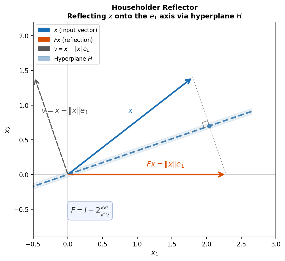Householder reflection: vector x reflected across the hyperplane H to align with e₁

The orthogonal projection of \( x \) onto \( H \) is \( Px = x - v(v^T x / v^T v) \). To reflect across \( H \) rather than project onto it, one must go twice as far:

\[ Fx = x - 2v \frac{v^T x}{v^T v}. \]

Therefore, the Householder reflector matrix is

\[ F = I - 2 \frac{vv^T}{v^T v}, \quad v = \|x\|e_1 - x. \]

One could alternatively reflect \( x \) to \( -\|x\|e_1 \), using \( v = -\|x\|e_1 - x \). Both choices zero the desired entries. For numerical stability, we choose the reflection that moves \( x \) farther from itself, thus avoiding cancellation error from subtracting nearby quantities:

• if \( x_1 > 0 \), choose the negative target \( -\|x\|e_1 \),
• if \( x_1 < 0 \), choose the positive target \( +\|x\|e_1 \).

This means \( v = \text{sign}(x_1)\|x\|e_1 + x \), where \( \text{sign}(x_1) \) picks the sign of \( x_1 \).

Two choices of sign in the Householder reflector

Alternative Derivation. One can also derive the Householder reflector by working backwards. Given a reflection operator \( F = I - 2vv^T/(v^T v) \) for some unknown \( v \), and demanding \( Fx \in \text{span}\{e_1\} \), it follows that \( v \in \text{span}\{e_1, x\} \). Setting \( v = x + \alpha e_1 \) for some unknown scalar \( \alpha \) and substituting into \( Fx \), one finds that \( Fx \in \text{span}\{e_1\} \) requires \( \alpha^2 - x^T x = 0 \), i.e., \( \alpha = \pm \|x\| \). Hence \( v = x \pm \|x\|e_1 \) and \( Fx = \mp \|x\|e_1 \).

19.2 Householder QR Factorization Algorithm

Algorithm 19.1 gives the QR factorization via Householder triangularization. At each outer step \( k \), the current column \( x = A(k:m, k) \) is extracted, the normalized reflection vector \( v_k = (x + \text{sign}(x_1)\|x\|e_1)/\|\cdots\| \) is formed, and then the reflector is applied to the active lower-right block via

\[ A(k:m, j) = A(k:m, j) - 2v_k(v_k^T A(k:m, j)), \quad j = k, k+1, \ldots, n. \]

Crucially, the algorithm does not explicitly build \( Q \), only the vectors \( v_k \). This is intentional: in practice we rarely need \( Q \) itself but only the products \( Q^T b \) or \( Qx \) (e.g., for least squares we solve \( Rx = Q^T b \). These products can be formed implicitly from the stored \( v_k \)’s in \( O(mn) \) flops, using the observation that \( Q^T = Q_n Q_{n-1} \cdots Q_1 \) and \( Q = Q_1 Q_2 \cdots Q_n \). One computes \( v(v^T b) \) rather than \( (vv^T)b \) to avoid forming the rank-one matrix \( vv^T \).

When an explicit \( Q \) is needed, it can be recovered by applying the implicit product to the columns of the identity: \( q_i = Qe_i \). For the reduced QR factorization, only the first \( n \) columns of \( I \) are needed.

Complexity. The work in the inner loop per outer step \( k \) is approximately \( 4(m-k+1)(n-k+1) \) flops. Summing over \( k = 1, \ldots, n \) gives a total of approximately

\[ \sum_{k=1}^{n} 4(m-k+1)(n-k+1) \approx 2mn^2 - \frac{2}{3}n^3. \]

For a square matrix (\( m = n \), flops(Householder) \( \approx \frac{4}{3}n^3 \), which is approximately \( 2 \times \) the cost of LU factorization and cheaper than Gram-Schmidt (which costs approximately \( 3 \times \) as much as LU).

Worked Example: QR via Householder

We perform QR factorization using Householder reflections on the same matrix \( A \) with first column \( (1, 2, 2)^T \). The goal in step 1 is to zero the second and third components of this column.

We take \( x = (1, 2, 2)^T \) with \( \|x\| = \sqrt{1 + 4 + 4} = 3 \). Since \( x_1 = 1 > 0 \), numerical stability dictates we use the plus sign: \( v = x + \text{sign}(x_1)\|x\|e_1 = (1,2,2)^T + 3(1,0,0)^T = (4,2,2)^T \). Computing \( v^T v = 16 + 4 + 4 = 24 \) and \( vv^T \), the Householder reflector is

\[ F_1 = I - \frac{2}{24} vv^T = \frac{1}{3}\begin{pmatrix} -1 & -2 & -2 \\ -2 & 2 & -1 \\ -2 & -1 & 2 \end{pmatrix}. \]

One can verify that \( F_1 x = -\|x\|e_1 = (-3, 0, 0)^T \), which is consistent with the numerically stable choice. Using the alternative \( v = (-2, 2, 2)^T \) (less stable) gives \( F_1 x = (3, 0, 0)^T \). Taking the second (positive) reflector as \( Q_1 \), applying it to \( A \) yields

\[ Q_1 A = \begin{pmatrix} 3 & 2 & 0 \\ 0 & -3 & \cdots \\ 0 & -4 & \cdots \end{pmatrix}. \]

In step 2, the active subvector for the second column is \( x = (-3, -4)^T \) with \( \|x\| = 5 \). Since \( x_1 = -3 < 0 \), we use \( v = x + (\text{sign}(-3)) \cdot 5 \cdot e_1 = (-3, -4)^T + (-5, 0)^T = (-8, -4)^T \). Computing \( v^T v = 64 + 16 = 80 \) gives

\[ F_2 = I - \frac{2}{80}\begin{pmatrix} 64 & 32 \\ 32 & 16 \end{pmatrix} = \begin{pmatrix} -3/5 & -4/5 \\ -4/5 & 3/5 \end{pmatrix}. \]

The full second Householder matrix is \( Q_2 = \text{diag}(1, F_2) \). Applying \( Q_2 \) to \( Q_1 A \) gives the upper triangular matrix

\[ R = Q_2 Q_1 A = \begin{pmatrix} 3 & 2 & 0 \\ 0 & 5 & 0 \\ 0 & 0 & \cdots \end{pmatrix}. \]

Since both \( Q_1 \) and \( Q_2 \) are symmetric (a special property of this particular construction, not of orthogonal matrices in general), \( Q = Q_1 Q_2 \). Computing this product gives

\[ Q = \begin{pmatrix} 1/3 & -14/15 & -2/15 \\ 2/3 & 1/3 & -2/3 \\ 2/3 & 2/15 & 11/15 \end{pmatrix}. \]

---

Givens Rotations

This lecture discusses the third and final common algorithm for QR factorization: Givens rotations. The key idea is to zero individual matrix entries selectively by applying orthogonal rotations in chosen coordinate planes.

20.1 Rotation Matrices in 2D

A vector in two dimensions can be rotated by angle \( \theta \) counterclockwise via multiplication by the rotation matrix

\[ R(\theta) = \begin{pmatrix} \cos\theta & -\sin\theta \\ \sin\theta & \cos\theta \end{pmatrix}. \]

This matrix is orthogonal: its columns are orthonormal by the identities \( \cos^2\theta + \sin^2\theta = 1 \) and \( \cos\theta \sin\theta - \cos\theta \sin\theta = 0 \). The transpose \( R(\theta)^T \) gives a clockwise rotation, i.e., the inverse operation. For example, rotating by \( \theta = \pi/4 \) applied to \( b = (1,0)^T \) yields \( a = Rb = (1/\sqrt{2}, 1/\sqrt{2})^T \).

20.2 Givens Rotation

A Givens rotation \( G(i, k, \theta) \) is an orthogonal matrix that is the identity everywhere except at the intersection of rows \( i \) and \( k \) with columns \( i \) and \( k \), where it contains a \( 2 \times 2 \) rotation block with \( c = \cos\theta \) and \( s = \sin\theta \). The transpose acts on a vector \( x \) as

\[ (G^T x)_j = \begin{cases} c x_i - s x_k & j = i \\ s x_i + c x_k & j = k \\ x_j & j \neq i, k \end{cases} \]

To force \( y_k = 0 \), we need \( s x_i + c x_k = 0 \), which is satisfied by choosing

\[ c = \frac{x_i}{\sqrt{x_i^2 + x_k^2}}, \quad s = \frac{-x_k}{\sqrt{x_i^2 + x_k^2}}. \]

The value of \( \theta \) itself is never needed explicitly when computing \( y = G^T x \). Also note that applying \( G(i, k, \theta)^T \) to a matrix \( A \) affects only rows \( i \) and \( k \) of \( A \).

Givens QR Factorization Process. To perform a QR factorization, zeros are introduced one at a time by working upwards along each column. For a \( 4 \times 3 \) matrix, one first applies \( G(3,4)^T \) to zero the \( (4,1) \) entry, then \( G(2,3)^T \) for the \( (3,1) \) entry, then \( G(1,2)^T \) for the \( (2,1) \) entry, and so on across subsequent columns.

The matrix \( Q \) is assembled from the product of the individual Givens matrices: if \( G_k^T \) denotes the \( k \)-th Givens rotation, then \( G_{\ell}^T \cdots G_1^T A = R \), so \( A = G_1 G_2 \cdots G_\ell R \) and therefore \( Q = G_1 G_2 \cdots G_\ell \).

In terms of complexity, flops(Givens QR) \( \approx 3mn^2 - n^3 \approx 1.5 \times \) flops(Householder QR). Givens QR is slower than Householder in general, but it is more flexible: it excels when only a few elements need to be zeroed. A prime example is an upper Hessenberg matrix, which has nonzeros only on and above the first subdiagonal. Givens QR factorizes an upper Hessenberg matrix using only \( n-1 \) Givens rotations (one per subdiagonal entry) at a total cost of approximately \( 3n^2 \) flops, far less than Householder QR would require.

20.3 Least Squares: Normal Equations vs. QR

Having seen all three QR algorithms (Gram-Schmidt, Householder, Givens), we compare the two main approaches to solving least squares problems: the normal equations and the QR factorization. The steps after computing \( A = QR \) are the same regardless of the method used to obtain it.

The drawback of the normal equations \( A^T A x = A^T b \) is poor conditioning. The accuracy of a linear system solution is governed by the condition number of the matrix being inverted, which here is \( \kappa(A^T A) \) rather than \( \kappa(A) \). This is often dramatically worse: for example, a matrix with \( \kappa(A) = 4 \times 10^8 \) can have \( \kappa(A^T A) \approx 16 \times 10^{16} \), essentially squaring the condition number.

The QR approach solves \( Rx = Q^T b \), and its accuracy depends on \( \kappa(R) \). Since \( \kappa_2(A) = \kappa_2(QR) = \kappa_2(R) \) (using the fact that \( \|Q\|_2 = 1 \) for matrices with orthonormal columns), the QR approach does not amplify the condition number. Therefore, despite its extra cost, the QR approach is preferred for potentially ill-conditioned problems, while the normal equations are acceptable when it is known that \( A \) is well-conditioned.

Worked Example: QR via Givens

We apply a single Givens rotation to zero out a targeted component of the vector \( x = (1, 2, 3, 4)^T \), using \( i = 2 \) and \( k = 4 \) (so the goal is to zero the fourth component).

First we compute the rotation parameters. With \( x_i = x_2 = 2 \) and \( x_k = x_4 = 4 \),

\[ c = \frac{x_i}{\sqrt{x_i^2 + x_k^2}} = \frac{2}{\sqrt{4 + 16}} = \frac{2}{\sqrt{20}} = \frac{1}{\sqrt{5}}, \quad s = \frac{-x_k}{\sqrt{x_i^2 + x_k^2}} = \frac{-4}{\sqrt{20}} = \frac{-2}{\sqrt{5}}. \]

The Givens matrix \( G(2, 4, \theta)^T \) is the identity except in rows 2 and 4: row 2 becomes \( (0, c, 0, -s) = (0, 1/\sqrt{5}, 0, 2/\sqrt{5}) \) and row 4 becomes \( (0, s, 0, c) = (0, -2/\sqrt{5}, 0, 1/\sqrt{5}) \). Note that this matrix is orthogonal but not symmetric, in contrast to Householder reflectors which are always symmetric.

Computing the product \( G^T x \): the first and third components are unchanged (\( y_1 = 1 \), \( y_3 = 3 \). For the \( i \)-th row:

\[ y_2 = c x_2 - s x_4 = \frac{1}{\sqrt{5}} \cdot 2 - \frac{-2}{\sqrt{5}} \cdot 4 = \frac{2 + 8}{\sqrt{5}} = \frac{10}{\sqrt{5}} = \sqrt{20}. \]

For the \( k \)-th row:

\[ y_4 = s x_2 + c x_4 = \frac{-2}{\sqrt{5}} \cdot 2 + \frac{1}{\sqrt{5}} \cdot 4 = \frac{-4 + 4}{\sqrt{5}} = 0. \]

Therefore \( G^T x = (1, \sqrt{20}, 3, 0)^T \). The targeted fourth component has been zeroed, and the second component equals \( \sqrt{x_2^2 + x_4^2} = \sqrt{20} \), confirming that the rotation preserves the overall length of the vector by combining the energy of the two affected components into a single one.

---

Eigenvalue Problems

So far this course has focused on solving linear systems and least-squares problems of the form \( Ax = b \). We now turn to eigenvalue problems, which have the form \( Ax = \lambda x \). This lecture begins with definitions and theory; much of this material is review from introductory linear algebra.

21.1 Eigenvalue Problem Definitions

Definition 21.1. Let \( A \in \mathbb{R}^{n \times n} \). A non-zero vector \( x \in \mathbb{R}^n \) is a (right) eigenvector with corresponding eigenvalue \( \lambda \in \mathbb{R} \) if \( Ax = \lambda x \).

Definition 21.2. The set of all eigenvalues of \( A \) is called its spectrum, denoted \( \Lambda(A) \).

Definition 21.3. The eigendecomposition of \( A \) is \( A = X\Lambda X^{-1} \), where \( X = [x_1 \; x_2 \; \cdots \; x_n] \) collects the eigenvectors as columns and \( \Lambda = \text{diag}(\lambda_1, \lambda_2, \ldots, \lambda_n) \) contains the corresponding eigenvalues. Equivalently, the eigendecomposition can be written as \( AX = X\Lambda \), since \( Ax_i = \lambda_i x_i \) for each \( i \). The existence of the eigendecomposition depends on the properties of \( A \).

21.2 Traditional Eigenvalue Problem Review

In introductory courses, eigenvalues are computed using the characteristic polynomial.

Definition 21.4. The characteristic polynomial of \( A \) is \( p_A(z) = \det(zI - A) \).

Theorem 21.1. \( \lambda \) is an eigenvalue of \( A \) if and only if \( p_A(\lambda) = 0 \).

The proof is direct: \( \lambda \) is an eigenvalue if and only if \( \lambda I - A \) is singular, i.e., \( \det(\lambda I - A) = 0 \). The fundamental theorem of algebra guarantees that \( p_A(z) \), a degree-\( n \) polynomial, has exactly \( n \) complex roots (not necessarily distinct), so \( A \) has \( n \) eigenvalues. Given an eigenvalue \( \lambda \), the corresponding eigenvectors are the null space of \( \lambda I - A \). Conversely, for every monic polynomial of degree \( n \), the companion matrix is a matrix whose eigenvalues are the polynomial’s roots.

Definition 21.5. The algebraic multiplicity of \( \lambda \) is the number of times it appears as a root of \( p_A(z) \).

Definition 21.6. The geometric multiplicity of \( \lambda \) is the dimension of the null space of \( \lambda I - A \).

When the algebraic multiplicity exceeds the geometric multiplicity, \( \lambda \) is called a defective eigenvalue, and \( A \) is called a defective matrix. Only non-defective matrices possess an eigendecomposition.

As an example, consider two matrices:

\[ A = 2I, \quad B = \begin{pmatrix} 2 & 1 & 0 \\ 0 & 2 & 1 \\ 0 & 0 & 2 \end{pmatrix}. \]

Both have characteristic polynomial \( p(z) = (z-2)^3 \) with algebraic multiplicity 3 for \( \lambda = 2 \). For \( A = 2I \), the null space of \( 2I - A = 0 \) is all of \( \mathbb{R}^3 \), so the geometric multiplicity is 3 and \( A \) is non-defective. For \( B \), only \( x = (1,0,0)^T \) spans the null space of \( 2I - B \), so the geometric multiplicity is 1 and \( B \) is defective.

21.3 Solving Eigenvalue Problems (Naïve Approach)

The characteristic polynomial approach suggests computing eigenvalues by finding roots of \( p_A(z) \). However, for polynomials of degree \( \geq 5 \), there is no closed-form formula analogous to the quadratic formula (Abel’s theorem). More importantly, polynomial root-finding is inherently ill-conditioned: a tiny perturbation in the polynomial’s coefficients can drastically change the roots. This motivates the iterative methods explored in subsequent lectures.

Conversely, for every monic polynomial \( p(z) = z^n + a_{n-1}z^{n-1} + \cdots + a_1 z + a_0 \), the companion matrix

\[ C = \begin{pmatrix} 0 & & & -a_0 \\ 1 & 0 & & -a_1 \\ & 1 & \ddots & \vdots \\ & & 1 & -a_{n-1} \end{pmatrix} \]

has characteristic polynomial equal to \( p(z) \), so its eigenvalues are exactly the roots of \( p \). This shows that the eigenvalue problem is at least as hard as polynomial root-finding — one cannot hope to solve it in closed form for general matrices. Nevertheless, iterative methods that work directly on the matrix (rather than on polynomial coefficients) can be both fast and numerically stable.

21.4 Gershgorin Circle Theorem

A useful tool for bounding eigenvalues without computing them is the following.

Theorem 21.2 (Gershgorin Circle Theorem). Let \( A \) be any square matrix. All eigenvalues \( \lambda \) of \( A \) lie in the union of \( n \) disks on the complex plane:

\[ |\lambda - a_{ii}| \leq R_i, \quad \text{where} \quad R_i = \sum_{j \neq i} |a_{ij}|. \]

The disk \( D(a_{ii}, R_i) \) is centered at the diagonal entry \( a_{ii} \) with radius equal to the sum of the absolute values of the off-diagonal entries in row \( i \).

Proof. Let \( Ax = \lambda x \) with \( x \neq 0 \). Choose the index \( p \) such that \( |x_p| = \|x\|_\infty \geq |x_j| \) for all \( j \). Since \( x_p \neq 0 \), we may scale so that \( |x_p| = 1 \). The \( p \)-th row of the eigenvalue equation gives \( \sum_{j=1}^{n} a_{pj} x_j = \lambda x_p \), so \( (\lambda - a_{pp}) x_p = \sum_{j \neq p} a_{pj} x_j \). Taking absolute values and applying the triangle inequality:

\[ |\lambda - a_{pp}| = \left|\sum_{j \neq p} a_{pj} x_j\right| \leq \sum_{j \neq p} |a_{pj}| |x_j| \leq \sum_{j \neq p} |a_{pj}| = R_p, \]

where the last inequality uses \( |x_j| \leq |x_p| = 1 \). Thus \( \lambda \) lies in the disk \( D(a_{pp}, R_p) \). The key insight is that if the off-diagonal entries of a row are small, the corresponding eigenvalue must lie close to the diagonal entry. For a diagonal matrix, the Gershgorin disks reduce to points and the eigenvalues can be read off exactly.

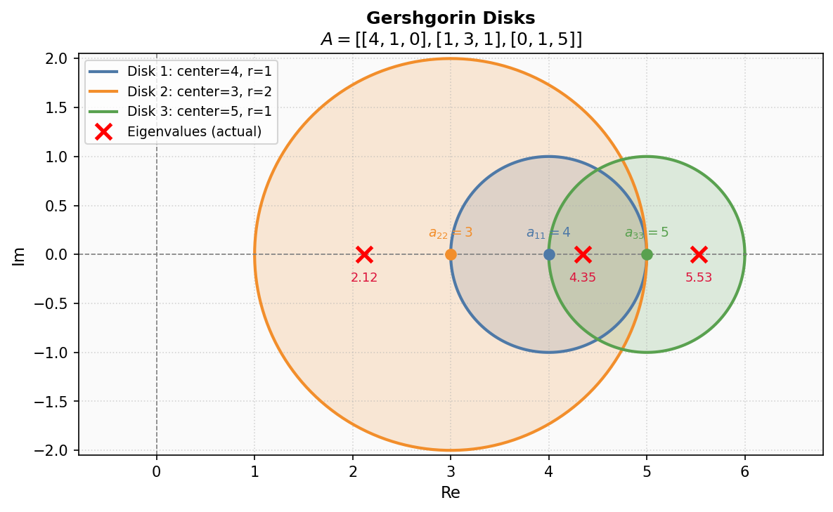Gershgorin disks in the complex plane containing all eigenvalues

21.5 Eigenvalue/Eigenvector Review Example

We find the eigenvalues and eigenvectors of

\[ A = \begin{pmatrix} 1 & 0 & 0 \\ 2 & -1 & 2 \\ 4 & -4 & 5 \end{pmatrix}. \]

The characteristic polynomial is

\[ p_A(\lambda) = \det(\lambda I - A) = (\lambda - 1)((\lambda+1)(\lambda-5) + 8) = (\lambda-1)(\lambda^2 - 4\lambda + 3) = (\lambda-1)^2(\lambda-3). \]

Thus \( \Lambda(A) = \{1, 3\} \) where \( \lambda = 1 \) has algebraic multiplicity 2.

For \( \lambda = 3 \): solving \( (3I - A)x = 0 \) gives \( x_1 = 0 \) and \( 4x_2 - 2x_3 = 0 \), so \( x_2 = x_3/2 \). An eigenvector is \( x_1 = (0, 1, 2)^T \).

For \( \lambda = 1 \): solving \( (I - A)x = 0 \) gives the single equation \( -x_1 + x_2 - x_3 = 0 \). The two-dimensional null space is spanned by \( x_2 = (1, 0, -1)^T \) and \( x_3 = (1, 1, 0)^T \), confirming that \( \lambda = 1 \) has geometric multiplicity 2 and the matrix is non-defective.

---

Power, Inverse, and Rayleigh Quotient Iterations

This lecture examines three iterative methods for finding eigenvalues of a matrix \( A \): power iteration, inverse iteration, and Rayleigh quotient iteration. We generally consider symmetric matrices (\( A^T = A \), which have real eigenvalues and a complete set of orthogonal unit eigenvectors \( \lambda_1, \lambda_2, \ldots, \lambda_n \) and \( q_1, q_2, \ldots, q_n \) with \( A = Q\Lambda Q^T \) where \( Q \) is orthogonal.

22.1 The Rayleigh Quotient

When given an approximation to an eigenvector, the corresponding eigenvalue can be estimated efficiently.

Definition 22.1. The Rayleigh quotient of a nonzero vector \( x \) with respect to \( A \) is

\[ r(x) = \frac{x^T A x}{x^T x}. \]

If \( x \) is an eigenvector, then \( r(x) = \lambda \) exactly. The Rayleigh quotient also has a least squares interpretation: it is the minimizer of \( \|x\alpha - Ax\|^2 \) over scalars \( \alpha \), as can be seen by forming the single-variable normal equations \( (x^T x)\alpha = x^T(Ax) \). A crucial property is that the Rayleigh quotient is second-order accurate in the eigenvector error.

Theorem 22.1. Let \( q_j \) be an eigenvector and \( x \approx q_j \). Then \( r(x) - r(q_j) = O(\|x - q_j\|^2) \) as \( x \rightarrow q_j \).

That is, the eigenvalue estimate is quadratically accurate in the eigenvector approximation. This motivates the methods that follow.

22.2 Power Iteration

Power iteration starts from an initial unit-norm vector \( v^{(0)} \) and repeatedly multiplies by \( A \) and normalizes:

\[ v^{(k)} = \frac{A v^{(k-1)}}{\|A v^{(k-1)}\|}. \]

The sequence converges to the eigenvector \( q_1 \) associated with the largest-magnitude eigenvalue. To see why, expand \( v^{(0)} \) in the eigenvector basis: \( v^{(0)} = c_1 q_1 + c_2 q_2 + \cdots + c_n q_n \). Then

\[ A^k v^{(0)} = \lambda_1^k \left( c_1 q_1 + c_2 \left(\frac{\lambda_2}{\lambda_1}\right)^k q_2 + \cdots + c_n \left(\frac{\lambda_n}{\lambda_1}\right)^k q_n \right). \]

When \( |\lambda_1| > |\lambda_2| \geq \cdots \) and \( c_1 = q_1^T v^{(0)} \neq 0 \), all ratio terms \( (\lambda_i/\lambda_1)^k \rightarrow 0 \) for \( i > 1 \), leaving \( A^k v^{(0)} \approx c_1 \lambda_1^k q_1 \). After normalization, this yields \( q_1 \).

Theorem 22.2 (Power Iteration Convergence). Under the above assumptions,

\[ \left\| v^{(k)} - (\pm q_1) \right\| = O\!\left(\left|\frac{\lambda_2}{\lambda_1}\right|^k\right), \quad |\lambda^{(k)} - \lambda_1| = O\!\left(\left|\frac{\lambda_2}{\lambda_1}\right|^{2k}\right). \]

Convergence is linear with factor \( |\lambda_2/\lambda_1| \), and is slow when the two largest eigenvalues have similar magnitudes. Note that the eigenvalue estimate converges at twice the rate of the eigenvector estimate, due to the quadratic accuracy of the Rayleigh quotient.

22.3 Inverse Iteration

Power iteration converges only to \( q_1 \). The inverse iteration is the power iteration applied to \( A^{-1} \) instead of \( A \). Since if \( Ax = \lambda x \) then \( A^{-1}x = (1/\lambda)x \), the eigenvalues of \( A^{-1} \) are the reciprocals of those of \( A \). The largest-magnitude eigenvalue of \( A^{-1} \) corresponds to the smallest-magnitude eigenvalue of \( A \), so inverse iteration converges to \( q_n \). In practice, one never explicitly forms \( A^{-1} \) but instead solves the linear system \( Aw = v^{(k-1)} \) at each step.

Shifting. To target a specific eigenvector \( q_j \), we apply inverse iteration to the shifted matrix \( B = A - \mu I \) for some scalar \( \mu \) near \( \lambda_j \). The shifted matrix has the same eigenvectors as \( A \) but with eigenvalues \( \lambda_i - \mu \). The eigenvalue of \( B \) with smallest magnitude is \( \lambda_j - \mu \approx 0 \), so inverse iteration on \( B \) converges to \( q_j \).

Theorem 22.3 (Inverse Iteration Convergence). If \( \lambda_J \) is the closest eigenvalue to \( \mu \) and \( \lambda_L \) is the next closest, then

\[ \left\| v^{(k)} - (\pm q_J) \right\| = O\!\left(\left|\frac{\mu - \lambda_J}{\mu - \lambda_L}\right|^k\right). \]

The convergence factor is the ratio of the two closest shifted eigenvalue magnitudes. Convergence can be made fast if \( \mu \) is chosen much closer to \( \lambda_J \) than to any other eigenvalue.

22.4 Rayleigh Quotient Iteration

The Rayleigh quotient iteration (RQI) combines inverse iteration with the Rayleigh quotient. It runs the shifted inverse iteration but updates \( \mu \) at each step to the current Rayleigh quotient estimate of the eigenvalue:

\[ \lambda^{(k)} = v^{(k)T} A v^{(k)}, \quad (A - \lambda^{(k)} I)w = v^{(k)}, \quad v^{(k+1)} = w/\|w\|. \]

Since the Rayleigh quotient gives a quadratically accurate eigenvalue estimate, and inverse iteration exploits a good eigenvalue estimate to refine the eigenvector, combining the two produces cubic convergence.

Theorem 22.4 (RQI Convergence). RQI converges cubically for almost all starting vectors: \( \|v^{(k+1)} - (\pm q_J)\| = O(\|v^{(k)} - (\pm q_J)\|^3) \). In practice, each iteration roughly triples the number of correct digits.

Computational Complexity. Power iteration costs \( O(n^2) \) flops per step (a matrix-vector product). Inverse iteration also costs \( O(n^2) \) per step because the matrix \( A - \mu I \) is fixed and can be pre-factored into \( LU \) once, leaving only forward/backward solves per iteration. Rayleigh quotient iteration costs \( O(n^3) \) per step because the matrix \( A - \lambda^{(k)} I \) changes at every step and must be factored fresh. For tridiagonal matrices, all three methods reduce to \( O(n) \) flops per step.

Worked Example: Rayleigh Quotient Iteration

Using the same matrix \( A = \begin{pmatrix} 21 & 7 & -1 \\ 5 & 7 & 7 \\ 4 & -4 & 20 \end{pmatrix} \) with eigenvalues \( \{8, 16, 24\} \) and initial vector \( v^{(0)} = (1, 1, 1)^T \), we apply RQI with the dynamically updated shift \( \lambda^{(k)} = r(v^{(k)}) \).

The initial Rayleigh quotient gives \( \lambda^{(0)} = 22 \). After one iteration of solving \( (A - 22I)w = v^{(0)} \), normalizing, and recomputing the Rayleigh quotient, we obtain \( \lambda^{(1)} = 24.0812 \). The second iteration gives \( \lambda^{(2)} = 24.0013 \), and the third gives \( \lambda^{(3)} = 24.00000017 \). The true eigenvalue is \( \lambda_1 = 24 \).

The cubic convergence is dramatic: the error drops from roughly 2 to 0.08 to 0.001 to \( 1.7 \times 10^{-7} \), with each iteration roughly cubing the previous error. Compare this with the power iteration example below, where \( \lambda^{(3)} \approx 23.87 \) still has an error of order \( 10^{-1} \) after the same number of iterations.

Worked Example: Power Iteration and Shifted Inverse Iteration

We apply power iteration and shifted inverse iteration to compute eigenvalues and eigenvectors of a matrix \( A \) with true eigenvalues including \( \lambda_1 = 24 \) and \( \lambda_2 = 16 \), starting from the initial vector \( v^{(0)} = (1, 1, 1)^T \).

Power Iteration. In the first iteration, we multiply by \( A \) to get \( w = Av^{(0)} = (27, 19, 20)^T \), then normalize to obtain \( v^{(1)} \approx (0.70, 0.49, 0.52)^T \). The Rayleigh quotient gives the eigenvalue estimate \( \lambda^{(1)} = v^{(1)T} Av^{(1)} \approx 23.32 \).

In the second iteration, \( w = Av^{(1)} \approx (17.62, 10.57, 11.19)^T \), normalizing yields \( v^{(2)} \approx (0.75, 0.45, 0.48)^T \), and the Rayleigh quotient gives \( \lambda^{(2)} \approx 23.73 \).

The third iteration gives \( w = Av^{(2)} \approx (18.5, 10.28, 10.71)^T \), \( v^{(3)} \approx (0.78, 0.43, 0.45)^T \), and \( \lambda^{(3)} \approx 23.87 \). The true values are \( q_1 \approx (0.8165, 0.4082, 0.4082)^T \) and \( \lambda_1 = 24 \). Each iteration brings the eigenvalue estimate closer to 24, and the eigenvector estimate is steadily converging to the true eigenvector.

Shifted Inverse Iteration. Now we target \( \lambda_2 = 16 \) using shift \( \mu = 15 \) and the same initial vector. We form \( B = A - 15I \) and apply inverse iteration to \( B \).

In iteration 1, solving \( Bw = v^{(0)} \) (never forming \( B^{-1} \) explicitly) gives \( w \approx (0.032, 0.16, 0.30)^T \). Normalizing yields \( v^{(1)} \approx (0.093, 0.46, 0.88)^T \), and the Rayleigh quotient gives \( \lambda^{(1)} \approx 19.2 \).

Iteration 2 gives \( w \approx (-0.33, 0.40, 0.76)^T \), \( v^{(2)} \approx (-0.36, 0.44, 0.83)^T \), and \( \lambda^{(2)} \approx 15.97 \). Iteration 3 yields \( v^{(3)} \approx (-0.40, 0.41, 0.82)^T \) and \( \lambda^{(3)} \approx 16.03 \). The true values are \( q_2 \approx (-0.4082, 0.4082, 0.8165)^T \) and \( \lambda_2 = 16 \). The convergence to both the eigenvalue and the eigenvector is clearly visible across the three iterations.

---

QR Iteration

In the previous lecture we found methods to compute a single eigenvalue/eigenvector pair at a time. Our next goal is to find all eigenvector/eigenvalue pairs simultaneously.

23.1 Similarity Transformations

Definition 23.1. Matrices \( A \) and \( B \) are similar if \( B = X^{-1}AX \) for some non-singular \( X \).

Definition 23.2. The map \( A \rightarrow X^{-1}AX \) is called a similarity transformation of \( A \).

Theorem 23.1. Similar matrices have the same characteristic polynomial, hence the same eigenvalues.

The proof uses the multiplicativity of the determinant: \( \det(zI - X^{-1}AX) = \det(X^{-1}) \det(zI - A) \det(X) = \det(zI - A) \). This means we can apply similarity transformations freely without changing the eigenvalues.

23.2 The QR Iteration Algorithm

The idea of QR iteration is to apply a sequence of similarity transformations to \( A \) that converge to a diagonal matrix whose entries are the eigenvalues. In 2000, the QR iteration was named one of the ten most important algorithms of the 20th century.

Given \( A^{(k-1)} \), we compute its QR factorization: \( A^{(k-1)} = Q^{(k)} R^{(k)} \), so \( R^{(k)} = Q^{(k)T} A^{(k-1)} \). Defining the next iterate as \( A^{(k)} = R^{(k)} Q^{(k)} \) yields a similarity transformation:

\[ A^{(k)} = R^{(k)} Q^{(k)} = Q^{(k)T} A^{(k-1)} Q^{(k)}. \]

Thus \( A^{(k-1)} \) and \( A^{(k)} \) are similar, preserving all eigenvalues. The basic QR iteration simply repeats: factor \( A^{(k-1)} = Q^{(k)} R^{(k)} \), then recombine as \( A^{(k)} = R^{(k)} Q^{(k)} \). Eventually \( A^{(k)} \) converges to a diagonal matrix containing the eigenvalues.

As the diagonal entries converge to eigenvalues, the accumulated product of \( Q \) matrices, denoted \( \mathbf{Q}^{(k)} = Q^{(1)} Q^{(2)} \cdots Q^{(k)} \), converges to the eigenvector matrix since \( A^{(k)} = (\mathbf{Q}^{(k)})^T A \mathbf{Q}^{(k)} \).

As a concrete illustration with \( A = \begin{pmatrix} 2 & 1 & 1 \\ 1 & 3 & 1 \\ 1 & 1 & 4 \end{pmatrix} \):

\[ A^{(1)} = \begin{pmatrix} 4.17 & 1.1 & -1.27 \\ 1.1 & 2 & 0 \\ -1.27 & 0 & 2.83 \end{pmatrix}, \quad A^{(2)} = \begin{pmatrix} 5.09 & 0.16 & 0.62 \\ 0.16 & 1.86 & -0.55 \\ 0.62 & -0.55 & 2.05 \end{pmatrix}, \quad \ldots \]

At each iteration the off-diagonal entries approach zero and the diagonal entries converge to the true eigenvalues \( \Lambda(A) = \{5.2143, 2.4608, 1.3249\} \).

23.3 Simultaneous (Block Power) Iteration

To understand why QR iteration works, we first analyze the simpler simultaneous iteration (also called block power iteration), in which power iteration is applied to several vectors at once while maintaining linear independence among them. Starting from an initial matrix \( \hat{Q}^{(0)} \in \mathbb{R}^{n \times p} \) with orthonormal columns, each step computes \( Z^{(k)} = A\hat{Q}^{(k-1)} \) and then takes the reduced QR factorization \( Z^{(k)} = \hat{Q}^{(k)} \hat{R}^{(k)} \) to re-orthonormalize the columns. The column spaces of \( \hat{Q}^{(k)} \) and \( Z^{(k)} \) are the same and both equal the column space of \( A^k \hat{Q}^{(0)} \).

The method relies on two assumptions: (1) the leading \( p+1 \) eigenvalues are distinct in absolute value, and (2) the leading principal submatrices of \( \hat{Q}^T V^{(0)} \) are non-singular. Under these conditions, simultaneous iteration converges linearly.

Theorem 23.2 (Simultaneous Iteration Convergence). With the above assumptions, as \( k \rightarrow \infty \),

\[ \|\hat{q}_j^{(k)} - (\pm q_j)\| = O(c^k), \quad j = 1, \ldots, p, \quad c = \max_{1 \leq k \leq p} \left|\frac{\lambda_{k+1}}{\lambda_k}\right| < 1. \]

23.4 Equivalence of QR Iteration and Simultaneous Iteration

The QR iteration (starting from \( A^{(0)} = A \) is in fact identical to the simultaneous iteration with \( \hat{Q}^{(0)} = I \) and \( p = n \). The following theorem makes this precise.

Theorem 23.3. The QR iteration and simultaneous iteration generate identical sequences of matrices satisfying

\[ A^k = \mathbf{Q}^{(k)} \mathbf{R}^{(k)} \quad \text{(QR factorization of } A^k\text{)}, \quad A^{(k)} = (\mathbf{Q}^{(k)})^T A \mathbf{Q}^{(k)} \quad \text{(similarity transform)}. \]

The proof proceeds by induction, showing the two properties hold at each step for both algorithms simultaneously. The base case \( k=0 \) is trivial. For the inductive step, both the simultaneous iteration path and the QR iteration path lead to the same updated \( \mathbf{Q}^{(k)} \) and \( \mathbf{R}^{(k)} \).

23.5 Convergence of QR Iteration

The connection \( A^k = \mathbf{Q}^{(k)} \mathbf{R}^{(k)} \) reveals that the QR iteration is computing an orthonormal basis for the column space of \( A^k \). Meanwhile, \( A^{(k)} = (\mathbf{Q}^{(k)})^T A \mathbf{Q}^{(k)} \) means the diagonal entries of \( A^{(k)} \) are the Rayleigh quotients of the column vectors of \( \mathbf{Q}^{(k)} \). As those columns approach the true eigenvectors, the Rayleigh quotients approach the eigenvalues. The off-diagonal entry \( A_{ij}^{(k)} = q_i^{(k)T} A q_j^{(k)} \) approaches \( q_i^T A q_j = q_i^T (\lambda_j q_j) \approx 0 \) by orthogonality.

Theorem 23.4 (QR Iteration Convergence). Assuming distinct eigenvalues in absolute value and a non-singular eigenvector matrix, \( A^{(k)} \) converges linearly to \( \text{diag}(\lambda_1, \ldots, \lambda_n) \) with constant

\[ C = \max_k \left|\frac{\lambda_{k+1}}{\lambda_k}\right|. \]

The methods discussed in this course for eigenvalue problems can be summarized as follows. We used the Rayleigh quotient to recover an eigenvalue given an approximate eigenvector. We used power iteration, inverse iteration, shifted inverse iteration, and Rayleigh quotient iteration to recover individual eigenvectors. We then introduced the QR iteration and simultaneous (block power) iteration as schemes for finding multiple eigenvector/eigenvalue pairs simultaneously.

---

Reduction to Hessenberg Form

Dense QR factorization at every step of the QR iteration algorithm costs approximately \( \frac{4}{3}n^3 \) flops, which is prohibitive for large matrices. This lecture develops a way to make the QR iteration practical by pre-processing \( A \) via a similarity transformation that introduces sparsity, thereby dramatically reducing the per-step cost of QR factorization.

24.1 Why Upper Hessenberg and Not Triangular?

One might hope to reduce \( A \) to triangular form by similarity transformations, since a triangular matrix is even cheaper for QR factorization. Consider attempting this with Householder reflections. Applying \( Q_1^T \) on the left zeros the entries below the diagonal in column 1. However, to maintain similarity we must also multiply by \( Q_1 \) on the right, and this right multiplication destroys the newly created zeros. The new zeros are immediately annihilated.

The way forward is to be less ambitious. We choose \( Q_1 \) so that it leaves the entire first row untouched. Then the right multiplication \( \cdot Q_1 \) does not disturb the first column, preserving the zeros we introduced. Specifically, the first Householder matrix takes the block form leaving the \( (1,1) \) entry fixed, while the lower-right block zeros entries in the second-through-last positions of column 1. This strategy reduces \( A \) to upper Hessenberg form: a matrix with zeros below the first subdiagonal.

24.2 Reduction to Upper Hessenberg

An upper Hessenberg matrix has nonzero entries only on and above the first subdiagonal. The reduction algorithm applies \( n-2 \) Householder-like operations via the similarity \( Q^T A Q \) where \( Q = Q_1 Q_2 \cdots Q_{n-2} \). Algorithm 24.1 gives the pseudocode. At each step \( k \):

1. Extract the subvector \( x = A(k+1:n, k) \) (the entries to be zeroed).
2. Form the normalized reflection vector \( v_k = \text{sign}(x_1)\|x\|e_1 + x \), \( v_k = v_k/\|v_k\| \).
3. Left-multiply: apply the reflector to rows \( k+1:n \) of \( A \) for all columns.
4. Right-multiply: apply the reflector to columns \( k+1:n \) of \( A \) for all rows.

The right-multiply step (step 4) is what differentiates this from the plain Householder QR. It is essential to maintain the similarity transformation and it does not destroy the zeros introduced in step 3 because the reflector acts on columns \( k+1 \) and beyond, leaving column \( k \) (where the zeros were introduced) undisturbed.

The cost of reducing \( A \) to upper Hessenberg form is approximately \( \frac{10}{3}n^3 \) flops. Crucially, this reduction is performed only once as a preprocessing step before the QR iteration begins.

24.3 Symmetric Case: Reduction to Tridiagonal

For symmetric matrices (\( A = A^T \), the similarity transformation preserves symmetry: \( (Q^T A Q)^T = Q^T A Q \). A matrix that is simultaneously symmetric and upper Hessenberg must be tridiagonal, since the upper Hessenberg structure requires zeros below the first subdiagonal, and symmetry then forces the corresponding zeros above the first superdiagonal as well. The cost of reducing a symmetric matrix to tridiagonal form is approximately \( \frac{4}{3}n^3 \) flops, significantly cheaper than the \( \frac{10}{3}n^3 \) for the general case.

The practical approach to computing all eigenvalues of a symmetric matrix is therefore a two-phase process:

Phase 1 (Direct): Reduce \( A \) to tridiagonal form \( T = Q^T A Q \) using Householder operations.

Phase 2 (Iterative): Apply the QR iteration to \( T \) until convergence to a diagonal matrix \( D \).

Phase 1 reduces the per-step QR factorization cost in Phase 2 from \( O(n^3) \) to \( O(n) \) for tridiagonal matrices (using Givens rotations, which need only zero \( n-1 \) subdiagonal entries). For general non-symmetric matrices, the reduction to upper Hessenberg in Phase 1 reduces the per-step QR factorization cost in Phase 2 to \( O(n^2) \).

24.4 Further Improvements to QR Iteration

The practical QR iteration algorithm incorporates two additional improvements beyond the Hessenberg reduction:

Shifting. By analogy with the shifted inverse iteration, applying shifts within the QR iteration achieves cubic (rather than linear) convergence rates. The shift at each step is chosen based on the current approximation to the eigenvalue, typically as the Rayleigh quotient of the bottom-right submatrix.

Deflation. Once a diagonal entry of \( A^{(k)} \) converges sufficiently close to an eigenvalue (detected by a small subdiagonal entry), that eigenvalue is considered “found.” The matrix is partitioned (deflated) into a smaller subproblem, and subsequent iterations operate only on the reduced matrix. This dramatically reduces the work once eigenvalues begin converging.

24.5 Historical Note

The implicit shifted QR algorithm was published by John Francis in 1961. He left the field of numerical analysis that same year and had no idea of the enormous influence of his work until he was tracked down in 2007. Concurrently and independently, the algorithm was invented by Vera Kublanovskaya, who continued to work in numerical analysis until her death in 2012. Together, their discovery gave the scientific computing community one of its most fundamental and widely-used algorithms.

Graph Laplacian

In the next two lectures we examine the application of eigenvalue problems to image segmentation. This lecture provides the foundational definitions and introduces the graph Laplacian. Spectral clustering, which uses the graph Laplacian’s eigendecomposition to identify clusters of “similar” or related elements, is the subject of Lecture 26. Segmentation tasks — identifying distinct parts of an image or shape — often rely on clustering. Image segmentation groups similar and nearby pixels; shape segmentation identifies distinct parts of a 3D object.

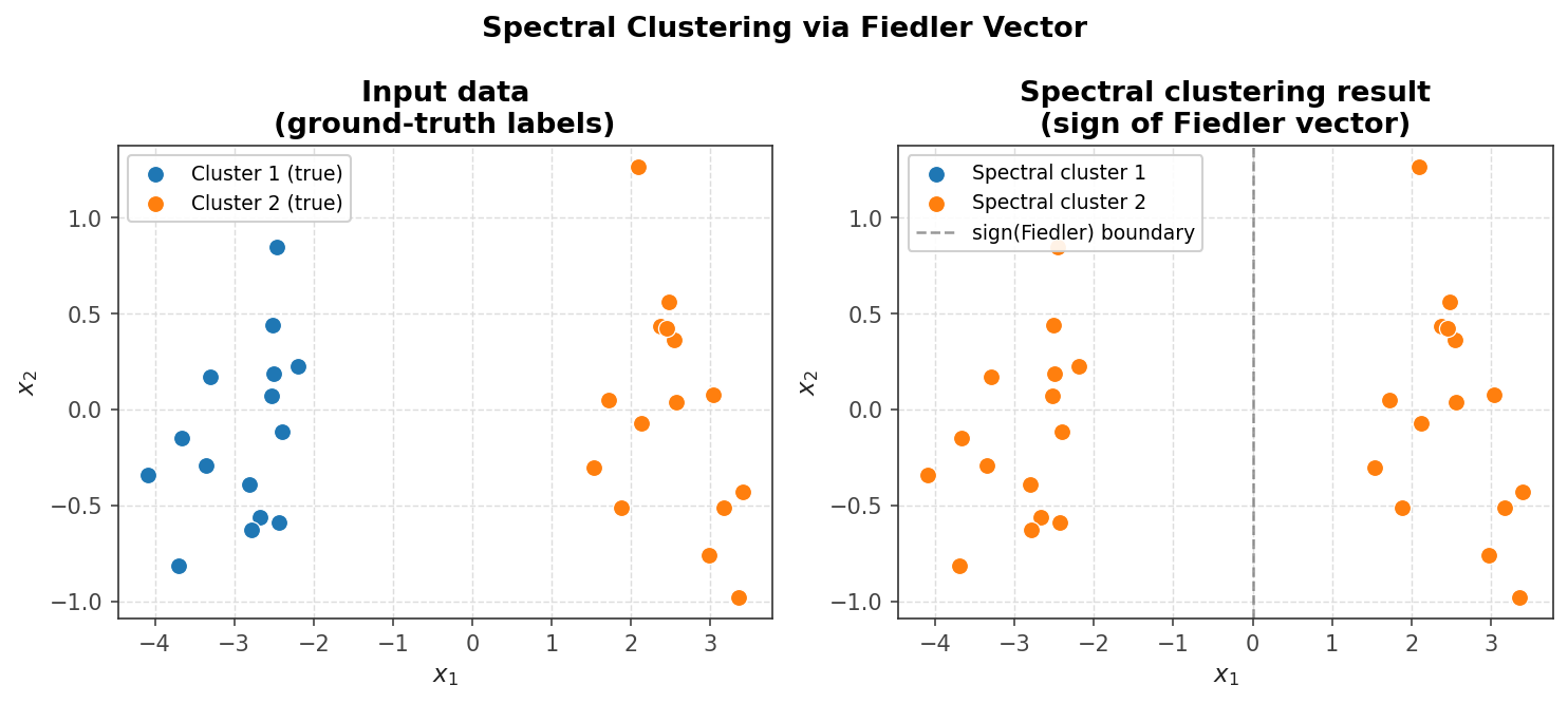Spectral clustering via the Fiedler vector separates two point-cloud clusters

25.1 Definitions

Consider an undirected graph \( G = (V, E) \), where \( V = \{v_1, \ldots, v_n\} \) is a set of vertices and \( E = \{e_{ij}\} \) is a set of edges, with \( e_{ij} \) denoting the edge between vertices \( v_i \) and \( v_j \).

Definition 25.1. The graph \( G \) is a weighted graph if edge \( e_{ij} \) has an associated weight \( w_{ij} \geq 0 \). The matrix \( W = [w_{ij}] \) is called the weighted adjacency matrix of the graph. Entries of \( W \) are zero wherever no edge joins \( v_i \) to \( v_j \), and equal to the edge weight wherever an edge exists.

Example undirected graph and its weighted version

For example, given the six-vertex graph in Figure 25.1, the weight matrix takes the form

\[ W = \begin{pmatrix} 0 & 1 & 1 & 2 & 0 & 0 \\ 1 & 0 & 0 & 3 & 0 & 0 \\ 1 & 0 & 0 & 4 & 0 & 2 \\ 2 & 3 & 4 & 0 & 2 & 0 \\ 0 & 0 & 0 & 2 & 0 & 0 \\ 0 & 0 & 2 & 0 & 0 & 0 \end{pmatrix}. \]

The definition of vertex degree must be modified from the unweighted setting to account for edge weights.

Definition 25.2. The degree of a vertex \( v_i \) is

\[ d_i = \sum_{j=1}^{n} w_{ij}, \]

and the degree matrix is \( D = \mathrm{diag}(d_i) \). For the example above, \( d_4 = 11 \) (the sum of the fourth row of \( W \), giving

\[ D = \mathrm{diag}(4, 4, 7, 11, 2, 2). \]

The indicator vector is a useful tool when working with a subset of the graph.

Definition 25.3. Given a subset \( A \subset V \), the indicator vector \( \mathbf{1}_A = (x_1, \ldots, x_n) \) has components

\[ x_i = \begin{cases} 1 & \text{if } v_i \in A, \\ 0 & \text{if } v_i \notin A. \end{cases} \]

Definition 25.4. Given two subsets \( A, B \subset V \), define \( W(A, B) \) as the total weight of all edges starting in \( A \) and ending in \( B \):

\[ W(A, B) = \sum_{i \in A,\ j \in B} w_{ij}. \]

For the subsets \( A = \{v_1, v_2, v_6\} \) and \( B = \{v_3, v_4, v_5\} \) in the example, one computes \( W(A,B) = w_{13} + w_{14} + w_{15} + w_{23} + w_{24} + w_{25} + w_{63} + w_{64} + w_{65} = 8 \).

There are two natural ways to measure the size of a subset \( A \subset V \).

\[ |A| = \text{number of vertices in } A, \]\[ \mathrm{vol}(A) = \sum_{i \in A} d_i = \text{sum of degrees of vertices in } A. \]

For the subsets above, \( |A| = 3 \), \( |B| = 3 \), \( \mathrm{vol}(A) = 10 \), and \( \mathrm{vol}(B) = 20 \).

25.2 Graph Laplacians

The graph Laplacian generalizes the finite difference discrete Laplacian operator to arbitrary graphs. Two variants are standard. The unnormalized graph Laplacian is

\[ L = D - W, \]

and the normalized graph Laplacian is

\[ \hat{L} = I - D^{-1/2} W D^{-1/2}. \]

For the example graph, direct subtraction gives

\[ L = D - W = \begin{pmatrix} 4 & -1 & -1 & -2 & 0 & 0 \\ -1 & 4 & 0 & -3 & 0 & 0 \\ -1 & 0 & 7 & -4 & 0 & -2 \\ -2 & -3 & -4 & 11 & -2 & 0 \\ 0 & 0 & 0 & -2 & 2 & 0 \\ 0 & 0 & -2 & 0 & 0 & 2 \end{pmatrix}. \]

The general matrix pattern closely resembles the finite difference discrete Laplacian: diagonal entries are all positive, off-diagonal entries are non-positive, and the sum of every row is zero.

Unnormalized Graph Laplacian. The following theorem records the key properties.

Theorem 25.1. The unnormalized graph Laplacian \( L \) satisfies:

1. \[ x^T L x = \frac{1}{2} \sum_{i,j=1}^{n} w_{ij}(x_i - x_j)^2. \]

2. \( L \) is symmetric and positive semi-definite.

3. The smallest eigenvalue of \( L \) is \( 0 \), with corresponding eigenvector the constant one vector \( \mathbf{1} = [1, 1, \ldots, 1]^T \).

4. \( L \) has \( n \) non-negative eigenvalues \( 0 = \lambda_1 \leq \lambda_2 \leq \cdots \leq \lambda_n \).

Proof. For property 1, expand \( x^T L x = x^T D x - x^T W x \), write out the sums, symmetrize using the fact that \( d_i = \sum_j w_{ij} \), and collect terms to obtain the squared-difference formula. For property 2, since \( w_{ij} \geq 0 \), property 1 immediately gives \( x^T L x \geq 0 \); symmetry follows because both \( D \) and \( W \) are symmetric. For property 3, since every row of \( L \) sums to zero, \( L \mathbf{1} = \mathbf{0} \), confirming eigenvalue \( 0 \). For property 4, positive semi-definiteness forces non-negative eigenvalues: if \( Ax = \lambda x \) then \( x^T Ax = \lambda \|x\|^2 \geq 0 \), so \( \lambda \geq 0 \).

Normalized Graph Laplacian. An analogous theorem holds for \( \hat{L} \).

Theorem 25.2. The normalized graph Laplacian \( \hat{L} \) satisfies:

1. \[ x^T \hat{L} x = \frac{1}{2} \sum_{i,j=1}^{n} w_{ij} \left( \frac{x_i}{\sqrt{d_i}} - \frac{x_j}{\sqrt{d_j}} \right)^2. \]

2. \( \hat{L} \) is symmetric and positive semi-definite.

3. The smallest eigenvalue of \( \hat{L} \) is \( 0 \), with eigenvector \( D^{1/2} \mathbf{1} \).

4. \( \hat{L} \) has \( n \) non-negative eigenvalues \( 0 = \lambda_1 \leq \lambda_2 \leq \cdots \leq \lambda_n \).

An important structural fact connects the multiplicity of the zero eigenvalue to the topology of the graph: the multiplicity \( k \) of the eigenvalue \( 0 \) for both \( L \) and \( \hat{L} \) equals the number of connected components \( A_1, \ldots, A_k \) in the graph. Finally, if the graph is a 2D grid with weights \( w_{ij} = 1 \), then the unnormalized graph Laplacian \( L \) is (up to a scalar multiple) exactly the usual 2D finite difference Laplacian.

---

Spectral Clustering

In this lecture we explore how graph Laplacians are used for clustering data. The central problem is to find a partition of a graph into parts such that the edges connecting different parts have very low total weight — that is, we seek a minimally weighted cut of the graph. This problem in full generality is NP-hard, so we relax it in a way that leads naturally to eigenvalue computations.

26.1 Clustering Using Graph Laplacians

The simplest approach, MinCut, finds a partition \( A_1, \ldots, A_k \) of the vertices that minimizes

\[ \mathrm{cut}(A_1, \ldots, A_k) = \frac{1}{2} \sum_{i=1}^{k} W(A_i, \bar{A}_i), \]

where \( \bar{A}_i \) is the complement of \( A_i \). While MinCut is computationally tractable, it yields poor partitions in practice: the minimum cut typically separates out individual vertices rather than finding large balanced groups. Better cuts encourage the parts to be large and balanced, which motivates dividing the cut weight by the size of each subset.

Definition 26.1. The RatioCut and the Ncut (normalized cut) are defined respectively by

\[ \mathrm{RatioCut}(A_1, \ldots, A_k) = \sum_{i=1}^{k} \frac{\mathrm{cut}(A_i, \bar{A}_i)}{|A_i|}, \]\[ \mathrm{Ncut}(A_1, \ldots, A_k) = \sum_{i=1}^{k} \frac{\mathrm{cut}(A_i, \bar{A}_i)}{\mathrm{vol}(A_i)}. \]

Relaxation of RatioCut via Graph Laplacian. Minimizing RatioCut and Ncut is NP-hard, but these problems can be rewritten in terms of the graph Laplacian, enabling a continuous relaxation. For the two-subset case, consider minimizing \( \mathrm{RatioCut}(A, \bar{A}) \). Define a vector \( x \in \mathbb{R}^n \) with components

\[ x_i = \begin{cases} +\sqrt{|\bar{A}|/|A|} & \text{if } v_i \in A, \\ -\sqrt{|A|/|\bar{A}|} & \text{if } v_i \in \bar{A}. \end{cases} \]

One can verify three results: (1) \( x^T L x = |V| \cdot \mathrm{RatioCut}(A, \bar{A}) \), (2) \( x^T \mathbf{1} = 0 \), and (3) \( \|x\|^2 = n \). The minimization problem therefore becomes

\[ \min_{A \subset V} x^T L x, \quad \text{subject to } x \perp \mathbf{1} \text{ and } \|x\| = \sqrt{n}. \]

This is still NP-hard because \( x \) is constrained to take only two specific values. However, if we relax the problem by allowing \( x \) to be any vector in \( \mathbb{R}^n \), the solution is the eigenvector corresponding to the second smallest eigenvalue of \( L \), known as the Fiedler vector. We recover the partition by thresholding: vertex \( v_i \) is placed in \( A \) if \( x_i \geq 0 \), and in \( \bar{A} \) if \( x_i < 0 \).

Relaxation of Ncut via Graph Laplacian. The same strategy applies to Ncut, but using the normalized graph Laplacian. The appropriately defined vector has components that involve \( \mathrm{vol}(A) \) and \( \mathrm{vol}(\bar{A}) \), and one can show that (1) \( x^T L x = \mathrm{vol}(V) \cdot \mathrm{Ncut}(A, \bar{A}) \), (2) \( (Dx)^T \mathbf{1} = 0 \), and (3) \( x^T D x = \mathrm{vol}(V) \). After the substitution \( y = D^{1/2} x \), the relaxed problem becomes minimizing \( y^T \hat{L} y \) subject to \( y \perp D^{1/2} \mathbf{1} \) and \( \|y\|^2 = \mathrm{vol}(V) \). The solution is again the Fiedler vector, but now of \( \hat{L} \), and thresholding at zero determines the two clusters.

26.2 K-means Clustering

The two-cluster approach above extends to \( k > 2 \) clusters through a combination with k-means clustering. Given a set of \( n \) data points \( \{p_j\} \), k-means finds the partition \( A_1, \ldots, A_k \) that minimizes

\[ \min_{A_i} \sum_{i=1}^{k} \sum_{p \in A_i} \|p - \mu_i\|^2, \]

where \( \mu_i \) is the mean (centroid) of the points in cluster \( A_i \). The algorithm iterates between two steps: assigning each point to its nearest centroid, then recomputing each centroid from its assigned points.

k-means clustering assigns each point to the nearest centroid

The k-means algorithm proceeds as follows. Start with initial guesses for the \( k \) means \( \{\mu_i\} \). Assign each point \( p \) to cluster \( A_i \) if \( p \) is closer to \( \mu_i \) than to any other centroid. Recompute the means \( \{\mu_i\} \) for all updated partitions. Repeat until convergence.

26.3 Spectral Clustering: Cuts and K-means Together

Why not apply k-means directly to the original data? Spectral clustering offers two key advantages over naive k-means: it accommodates more general notions of similarity (not just Euclidean distance) and it can identify non-convex clusters that Euclidean-distance-based methods would miss. The full spectral clustering pipeline combines the graph-Laplacian relaxation with k-means.

Intuitively, spectral clustering proceeds as follows. First, interpret the input data as a graph and choose weights \( W \) to encode the desired notion of similarity. Second, use the eigenvectors of the graph Laplacian to map each vertex to a point in \( \mathbb{R}^k \). Third, apply k-means to cluster those embedded points.

More concretely, the unnormalized spectral clustering algorithm is:

1. Construct the unnormalized graph Laplacian \( L \).
2. Compute the first \( k \) eigenvectors \( q_1, q_2, \ldots, q_k \) of \( L \) (those corresponding to the \( k \) smallest eigenvalues).
3. Form the matrix \( Q_k = [q_1, \ldots, q_k] \). Let \( p_i \in \mathbb{R}^k \) be the vector given by row \( i \) of \( Q_k \).
4. Apply k-means to the \( n \) points \( \{p_i\} \) in \( \mathbb{R}^k \).

The normalized version replaces \( L \) with \( \hat{L} \), and normalizes the row vectors so that each point used in k-means is \( p_i = p_i / \|p_i\| \).

Choosing Weights \( W \). The choice of weight matrix encodes problem-specific similarity. Typically, non-zero weights are assigned only between a small neighborhood of graph neighbors, which keeps the Laplacian sparse and makes eigendecomposition cheaper. For image segmentation, pixels serve as graph vertices and nearby pixels are connected by edges. A natural weight between pixels \( i \) and \( j \) combines spatial proximity and intensity similarity:

\[ w_{ij} = \exp\!\left( -\frac{\|x_i - x_j\|^2}{\sigma^2_{\mathrm{dist}}} \right) \exp\!\left( -\frac{\|I_i - I_j\|^2}{\sigma^2_{\mathrm{int}}} \right), \]

where \( x_i \) is the spatial position of pixel \( i \), \( I_i \) its intensity, and \( \sigma^2_{\mathrm{dist}} \), \( \sigma^2_{\mathrm{int}} \) are tunable parameters controlling the relative importance of the two terms.

26.4 Other Applications

Spectral methods based on graph Laplacians find broad use beyond image segmentation. In geometric mesh processing, eigenvectors of Laplacians defined on 3D triangle meshes provide a spectral basis for analyzing and processing shapes. In motion analysis, the eigenfunctions of the vector Laplacian form a basis of divergence-free fields that capture distinct spatial scales of vorticity in fluids or solids, enabling efficient simulation by working in a low-dimensional spectral basis. Another classic example is the analysis of vibrating membranes, where the eigenmodes of the Laplacian on the domain determine the natural frequencies of oscillation.

---

Singular Value Decomposition

With this lecture we arrive at the last of the course’s four main matrix decompositions: LU/Cholesky, QR, eigendecomposition, and finally the Singular Value Decomposition (SVD). The SVD is in many respects the most powerful and universally applicable of these factorizations.

27.1 Geometric Motivation: \( AV = U\Sigma \)

The image of the unit hypersphere \( S \) in \( \mathbb{R}^n \) under any \( m \times n \) matrix transformation \( A \) is a hyperellipse in \( \mathbb{R}^m \). The factors by which the sphere is scaled in each of the principal semi-axes of this ellipse are called the singular values of \( A \), denoted \( \sigma_i \), ordered so that \( \sigma_1 \geq \sigma_2 \geq \cdots \geq \sigma_n \geq 0 \). All singular values are non-negative.

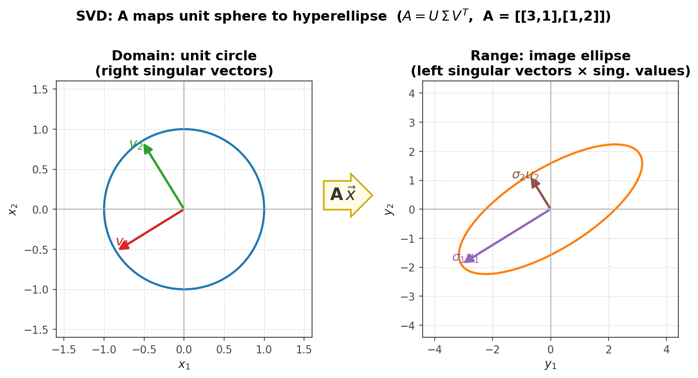The matrix A maps the unit sphere to a hyperellipse; singular vectors label the axes

The \( n \) left singular vectors \( u_i \) are the unit vectors in the directions of the principal semi-axes of the ellipse. The \( n \) right singular vectors \( v_i \) are the pre-images of the \( u_i \) under \( A \), satisfying

\[ A v_j = \sigma_j u_j, \quad j = 1, 2, \ldots, n. \]

Writing this column-by-column in matrix form defines the reduced (economy) SVD:

\[ A\underbrace{[v_1 \; v_2 \; \cdots \; v_n]}_{V,\ n\times n} = \underbrace{[u_1 \; u_2 \; \cdots \; u_n]}_{\hat{U},\ m\times n} \underbrace{\begin{pmatrix}\sigma_1 & & \\ & \ddots & \\ & & \sigma_n\end{pmatrix}}_{\hat{\Sigma},\ n\times n}, \]

or equivalently, since \( V \) is orthonormal, \( A = \hat{U} \hat{\Sigma} V^T \).

Reduced SVD: Û (m×n), Σ̂ (n×n), Vᵀ (n×n)

The full SVD is obtained by augmenting \( \hat{U} \) with \( m - n \) additional orthonormal columns to form a square \( m \times m \) orthogonal matrix \( U \), and padding \( \hat{\Sigma} \) with \( m - n \) zero rows to form \( \Sigma \), yielding \( A = U \Sigma V^T \).

Full SVD: U (m×m), Σ (m×n), Vᵀ (n×n)

Every matrix \( A \in \mathbb{R}^{m \times n} \) has a singular value decomposition; the singular values are uniquely determined. For square matrices with distinct singular values, the left and right singular vectors are also unique up to sign. It is instructive to compare the SVD with the eigendecomposition:

\[ A = U \Sigma V^T \quad \text{vs.} \quad A = X \Lambda X^{-1}. \]

Both decompositions diagonalize a matrix. The SVD uses two separate orthonormal bases, \( U \) and \( V \), while the eigendecomposition uses one basis of eigenvectors (which are not orthonormal in general). The SVD always exists — even for rectangular matrices — whereas the eigendecomposition may not.

27.2 Properties of the SVD

The following theorems collect the fundamental properties. Throughout, \( A \in \mathbb{R}^{m \times n} \) and \( r \) denotes the number of non-zero singular values.

Theorem 27.1. \( \mathrm{rank}(A) = r \).

Proof. The rank of a diagonal matrix equals its number of non-zero diagonal entries. Since \( U \) and \( V \) are full rank, \( \mathrm{rank}(A) = \mathrm{rank}(\Sigma) = r \).

Theorem 27.2. \( \mathrm{range}(A) = \mathrm{span}\{u_1, \ldots, u_r\} \) and \( \mathrm{null}(A) = \mathrm{span}\{v_{r+1}, \ldots, v_n\} \).

Proof. For the null space, if \( x \in \mathrm{span}\{v_{r+1}, \ldots, v_n\} \) then \( x = \sum_{i=r+1}^{n} w_i v_i \) and \( Ax = \sum_{i=r+1}^n w_i (Av_i) \). But \( Av_i = U\Sigma V^T v_i = U\Sigma e_i = 0 \) for \( i > r \), since those diagonal entries of \( \Sigma \) are zero. Therefore \( Ax = 0 \).

Theorem 27.3. \( \|A\|_2 = \sigma_1 \) and \( \|A\|_F = \sqrt{\sigma_1^2 + \sigma_2^2 + \cdots + \sigma_r^2} \).

Proof. Compute \( A^T A = V\Sigma^2 V^T \). Since this is similar to \( \Sigma^2 \), we have \( \lambda_{\max}(A^T A) = \sigma_1^2 \), giving \( \|A\|_2 = \sigma_1 \). For the Frobenius norm, use the trace identity \( \|A\|_F^2 = \mathrm{tr}(A^T A) = \mathrm{tr}(V\Sigma^2 V^T) = \mathrm{tr}(\Sigma^2) = \sigma_1^2 + \cdots + \sigma_r^2 \).

Theorem 27.4. The non-zero singular values of \( A \) are the square roots of the non-zero eigenvalues of \( A^T A \) (or equivalently \( A A^T \), since both are similar to \( \Sigma^2 \).

Theorem 27.5. If \( A = A^T \), then the singular values satisfy \( \sigma(A) = \{|\lambda| : \lambda \in \Lambda(A)\} \). In particular, if \( A \) is symmetric positive definite, then \( \sigma(A) = \Lambda(A) \).

Proof. Real symmetric matrices have an eigendecomposition \( A = Q\Lambda Q^T \) with orthogonal \( Q \). Construct the SVD as \( A = Q|\Lambda|\mathrm{sign}(\Lambda)Q^T \), identifying \( U = Q \), \( \Sigma = |\Lambda| \), and \( V^T = \mathrm{sign}(\Lambda)Q^T \).

Theorem 27.6. The condition number of \( A \in \mathbb{R}^{n \times n} \) is

\[ \kappa_2(A) = \frac{\sigma_1}{\sigma_n}. \]

Proof. Since \( A = U\Sigma V^T \), we have \( A^{-1} = V\Sigma^{-1}U^T \), so \( \|A^{-1}\|_2 = 1/\sigma_n \), and \( \kappa_2(A) = \|A\|_2 \|A^{-1}\|_2 = \sigma_1/\sigma_n \).

27.3 Computing the SVD — First Attempt

A naive approach to computing the SVD exploits the relation

\[ A^T A = V\Sigma^2 V^T, \]

which is an eigendecomposition of \( A^T A \). This suggests the following algorithm: (1) form \( A^T A \), (2) compute its eigendecomposition \( A^T A = V\Lambda V^T \), (3) set \( \Sigma = \sqrt{\Lambda} \), and (4) recover \( U \) by QR-factoring the product \( AV \) to obtain \( AV = QR \), then set \( U = Q \) and verify that \( R = \Sigma \).

Unfortunately, this naive method is inaccurate. The error in computed singular values satisfies

\[ |\tilde{\sigma}_k - \sigma_k| = O(\|A\|_2 / \sigma_k), \]

which can be very large for small singular values. The root cause is the same as squaring the condition number when solving least-squares via the normal equations: forming \( A^T A \) effectively squares the condition number, degrading accuracy. A more stable approach is presented in Lecture 28.

Worked Example: SVD Computation

We will find the singular value decomposition of the matrix

\[ A = \begin{pmatrix} 0 & -1/2 \\ 3 & 0 \\ 0 & 0 \end{pmatrix} \]

using three different methods.

Method 1: via \( A^T A \). We first compute

\[ A^T A = \begin{pmatrix} 0 & 3 & 0 \\ -1/2 & 0 & 0 \end{pmatrix} \begin{pmatrix} 0 & -1/2 \\ 3 & 0 \\ 0 & 0 \end{pmatrix} = \begin{pmatrix} 9 & 0 \\ 0 & 1/4 \end{pmatrix}. \]

From the lecture notes we know that \( A^T A = V\Sigma^2 V^T \). Since \( A^T A \) is already diagonal, we can read off the eigenvalues immediately: \( \lambda_1 = 9 \) and \( \lambda_2 = 1/4 \). The eigenvector matrix is just the identity, so \( v_1 = (1, 0)^T \) and \( v_2 = (0, 1)^T \), giving \( V = I \). Taking square roots gives \( \sigma_1 = \sqrt{9} = 3 \) and \( \sigma_2 = \sqrt{1/4} = 1/2 \), so

\[ \hat{\Sigma} = \begin{pmatrix} 3 & 0 \\ 0 & 1/2 \end{pmatrix}. \]

To find \( \hat{U} \) we use \( \hat{U} \hat{\Sigma} = AV = AI = A \). Equating column by column: \( 3 u_1 \) equals the first column of \( A \), which is \( (0, 3, 0)^T \), so \( u_1 = (0, 1, 0)^T \). Likewise, \( (1/2) u_2 \) equals the second column of \( A \), which is \( (-1/2, 0, 0)^T \), so \( u_2 = (-1, 0, 0)^T \). This yields the reduced SVD with \( \hat{U} = [u_1 \; u_2] \).

Method 2: via \( A A^T \). The same type of steps apply, but now the matrix algebra involves the \( 3\times 3 \) matrix \( AA^T \) and the left singular vectors are extracted directly from its eigendecomposition, followed by recovery of \( V \).

Method 3: geometric intuition. Since \( A \) has such a simple structure — exactly one non-zero entry in each column — we can reason directly about the range of \( A \). The range of \( A \) equals the span of the left singular vectors \( u_1 \) and \( u_2 \). The nonzero in the second row of the first column tells us \( u_1 = (0, 1, 0)^T \); the nonzero in the first row of the second column gives \( u_2 = (1, 0, 0)^T \) (or its negative). These are orthonormal as required. The lengths of the principal axes are the magnitudes of the entries, namely \( \sigma_1 = 3 \) and \( \sigma_2 = 1/2 \). Substituting into the defining equation \( A v_1 = \sigma_1 u_1 \) yields \( v_1 = (1, 0)^T \), and from \( A v_2 = \sigma_2 u_2 \) we get \( v_2 = (0, -1)^T \). Therefore,

\[ A = \underbrace{\begin{pmatrix} 0 & 1 \\ 1 & 0 \\ 0 & 0 \end{pmatrix}}_{\hat{U}} \underbrace{\begin{pmatrix} 3 & 0 \\ 0 & 1/2 \end{pmatrix}}_{\hat{\Sigma}} \underbrace{\begin{pmatrix} 1 & 0 \\ 0 & -1 \end{pmatrix}}_{V^T}. \]

This is the same SVD as in Method 1, but with the sign flip absorbed into \( V \) rather than \( \hat{U} \). Both are valid, reflecting the sign ambiguity inherent in singular vectors.

---

Alternative Formulation of SVD

Recall that the SVD decomposes any matrix \( A \) into \( U\Sigma V^T \), where \( \Sigma \) is diagonal with non-negative entries and \( U \), \( V \) are orthogonal. The naive approach from Lecture 27 computes the SVD via the eigendecomposition of \( A^T A \), but this is numerically unstable. In this lecture we develop a more stable method, prove the existence of the SVD for all matrices, and describe how to accelerate the computation in practice.

28.1 Alternative Formulation

Assume \( A \in \mathbb{R}^{n \times n} \). Consider the \( 2n \times 2n \) symmetric matrix

\[ H = \begin{pmatrix} 0 & A^T \\ A & 0 \end{pmatrix}. \]

By computing the eigendecomposition \( H = Q\Lambda Q^T \), one can extract the singular values and vectors of \( A \). The key relationship is \( \sigma_A = |\lambda_H| \), with \( U \) and \( V \) recoverable from the eigenvectors.

To see why, recall that \( A = U\Sigma V^T \) implies \( AV = U\Sigma \) and \( A^T U = V\Sigma \). Direct multiplication shows

\[ \begin{pmatrix} 0 & A^T \\ A & 0 \end{pmatrix} \begin{pmatrix} V & V \\ U & -U \end{pmatrix} = \begin{pmatrix} V & V \\ U & -U \end{pmatrix} \begin{pmatrix} \Sigma & 0 \\ 0 & -\Sigma \end{pmatrix}, \]

which is an eigendecomposition \( HQ = Q\Lambda \) of \( H \). (The columns of \( Q \) must be normalized for orthogonality.)

The algorithm is then:

1. Form \( H = \begin{pmatrix} 0 & A^T \\ A & 0 \end{pmatrix} \).
2. Compute the eigendecomposition \( HQ = Q\Lambda \).
3. Set \( \sigma_A = |\lambda_H| \).
4. Extract \( U \) and \( V \) from \( Q \), normalizing for orthogonality.

This algorithm is preferable with respect to stability. The error in computed singular values satisfies \( |\tilde{\sigma}_k - \sigma_k| = O(\varepsilon_{\mathrm{machine}} \|A\|) \), compared to \( O(\varepsilon_{\mathrm{machine}} \|A\|^2 / \sigma_k) \) for the \( A^T A \) approach. Practical algorithms extend this idea to non-square matrices, but without explicitly forming the large matrix \( H \).

28.2 Proof of Existence of SVD

Claim. Every matrix \( A \in \mathbb{R}^{m \times n} \) has a singular value decomposition.

Proof (by induction on min(\( m, n \)). Let \( \sigma_1 = \|A\|_2 \). Choose a unit vector \( v_1 \) achieving \( \|Av_1\| = \|A\|_2 = \sigma_1 \), and set \( u_1 = Av_1 / \sigma_1 \). Extend \( u_1 \) and \( v_1 \) to orthonormal bases \( U_1 \) and \( V_1 \) of \( \mathbb{R}^m \) and \( \mathbb{R}^n \) respectively. Then

\[ U_1^T A V_1 = \begin{pmatrix} \sigma_1 & w^T \\ 0 & B \end{pmatrix}, \]

where the bottom-left block is zero because \( u_i^T A v_1 = \sigma_1 u_i^T u_1 = 0 \) for all \( i \neq 1 \). To show \( w = 0 \), apply the induced norm definition: for the vector \( (\sigma_1, w^T w)^{1/2} \) scaled appropriately, one finds that \( \|S\|_2 \geq \sqrt{\sigma_1^2 + w^T w} \). But since \( U_1 \) and \( V_1 \) are orthogonal, \( \|S\|_2 = \|A\|_2 = \sigma_1 \), forcing \( w = 0 \). Therefore

\[ U_1^T A V_1 = \begin{pmatrix} \sigma_1 & 0 \\ 0 & B \end{pmatrix}. \]

For \( m = 1 \) or \( n = 1 \) this completes the proof. For larger matrices, by the inductive hypothesis the SVD of \( B \) exists: \( B = U_2 \Sigma_2 V_2^T \). Substituting gives

\[ A = U_1 \begin{pmatrix} 1 & 0 \\ 0 & U_2 \end{pmatrix} \begin{pmatrix} \sigma_1 & 0 \\ 0 & \Sigma_2 \end{pmatrix} \begin{pmatrix} 1 & 0 \\ 0 & V_2 \end{pmatrix}^T V_1^T, \]

which is an SVD of \( A \). The SVD therefore always exists.

28.3 Stability Comparison

Assume we use a stable eigenvalue algorithm (such as QR iteration) satisfying \( |\tilde{\lambda}_k - \lambda_k| = O(\varepsilon_{\mathrm{machine}} \|A\|) \). Applying this to the augmented matrix \( H \) gives

\[ |\tilde{\sigma}_k - \sigma_k| = O(\varepsilon_{\mathrm{machine}} \|H\|) = O(\varepsilon_{\mathrm{machine}} \|A\|). \]

In contrast, applying the same eigenvalue routine to \( A^T A \) yields \( |\tilde{\lambda}_k - \lambda_k| = O(\varepsilon_{\mathrm{machine}} \|A^T A\|) \approx O(\varepsilon_{\mathrm{machine}} \|A\|^2) \). Converting eigenvalues to singular values by taking square roots introduces a further factor of \( 1/\sigma_k \), giving \( |\tilde{\sigma}_k - \sigma_k| = O(\varepsilon_{\mathrm{machine}} \|A\|^2 / \sigma_k) \), which is very inaccurate for small singular values.

28.4 Golub-Kahan Bidiagonalization

In practice, SVD computation is accelerated by a two-phase strategy analogous to the reduction to Hessenberg form used before QR iteration for eigenvalues. The idea is to first reduce \( A \) to a bidiagonal matrix \( B \) (non-zero entries only on the main diagonal and the superdiagonal), then extract the SVD from \( B \) iteratively.

Unlike the eigendecomposition, the SVD does not require maintaining a similarity transformation: we need only \( U^T_{\text{left}} A V_{\text{right}} = B \), which allows applying different Householder reflectors on the left and right at each step. This flexibility makes it straightforward to zero out sub-diagonal entries from the left and then super-super-diagonal entries from the right in alternation.

Bidiagonalization uses \( n \) Householder reflectors on the left and \( n-2 \) on the right. Its cost is approximately \( 4mn^2 - \frac{4}{3}n^3 \) flops. In practice the bidiagonalization phase at cost \( O(mn^2) \) dominates over the subsequent iterative phase at cost \( O(n^2) \). The SVD is therefore more expensive than other factorizations, but it is the most numerically stable option for ill-conditioned or rank-deficient matrices.

Worked Example: Alternative SVD via the Augmented Matrix \( H \)

We demonstrate the alternative approach on the same matrix

\[ A = \begin{pmatrix} 0 & -1/2 \\ 3 & 0 \\ 0 & 0 \end{pmatrix}. \]

The first step is to construct the augmented matrix \( H \). Since \( A \) is \( 3 \times 2 \) we form a \( 5 \times 5 \) symmetric matrix by placing zeros in the upper-left \( 3 \times 3 \) block and upper-right \( 2 \times 2 \) block, placing \( A \) in the lower-left \( 3 \times 2 \) block, and placing \( A^T \) in the upper-right \( 2 \times 3 \) block, with the remaining lower-right entry zero.

Using MATLAB (or any numerical eigenvalue solver) to compute the eigendecomposition of \( H \), one obtains the eigenvector matrix

\[ Q = \frac{1}{\sqrt{2}} \begin{pmatrix} 1 & 0 & 0 & 1 & 0 \\ 0 & 1 & 1 & 0 & 0 \\ 0 & 1 & -1 & 0 & 0 \\ -1 & 0 & 0 & 1 & 0 \\ 0 & 0 & 0 & 0 & \sqrt{2} \end{pmatrix} \]

with eigenvalues \( \Lambda = \{-3, -1/2, 1/2, 3\} \) (and a fifth eigenvalue of zero). From the theory we know that the columns of \( Q \) have the block form \( (v, v, u, -u) \) corresponding to paired positive and negative singular values. To form a valid SVD we select the columns corresponding to the positive singular values, namely \( \sigma_1 = 3 \) and \( \sigma_2 = 1/2 \), keeping in mind the sign convention and the eigenvector sign ambiguity.

Reading off the appropriate blocks: \( v_1 = (1, 0)^T \) and \( u_1 = (0, 1, 0)^T \) correspond to \( \sigma_1 = 3 \); \( v_2 \) and \( u_2 = (-1, 0, 0)^T \) correspond to \( \sigma_2 = 1/2 \). Collecting results:

\[ U = \begin{pmatrix} 0 & -1 \\ 1 & 0 \\ 0 & 0 \end{pmatrix}, \quad V = \begin{pmatrix} 1 & 0 \\ 0 & 1 \end{pmatrix} = I, \quad \Sigma = \begin{pmatrix} 3 & 0 \\ 0 & 1/2 \end{pmatrix}. \]

This is consistent with the result from Lecture 27’s worked example, up to the sign convention for the columns of \( U \).

---

Low Rank Approximation

The singular value decomposition expresses any matrix \( A \) as a sum of rank-one matrices. Truncating this sum yields the best possible low-rank approximation of \( A \), a fact with far-reaching applications in data compression, image processing, and data analysis.

Theorem 29.1. Any matrix \( A \) with \( r \) non-zero singular values can be written as a sum of \( r \) rank-one matrices:

\[ A = \sum_{j=1}^{r} \sigma_j u_j v_j^T. \]

Proof. From \( A = U\Sigma V^T \) and the block structure of the matrix product, expanding column by column gives \( A = \sigma_1 u_1 v_1^T + \cdots + \sigma_r u_r v_r^T \).

The rank-\( k \) approximation of \( A \) is defined by keeping only the first \( k \) terms:

\[ A_k = \sum_{j=1}^{k} \sigma_j u_j v_j^T = U_k \Sigma_k V_k^T, \]

where \( U_k \), \( \Sigma_k \), and \( V_k \) consist of the first \( k \) columns of \( U \), the leading \( k \times k \) block of \( \Sigma \), and the first \( k \) columns of \( V \) respectively. The Eckart-Young theorem shows that \( A_k \) is optimal.

Theorem 29.2 (Eckart-Young). Among all matrices \( B \) with \( \mathrm{rank}(B) \leq k \),

\[ \|A - A_k\|_2 = \inf_{\mathrm{rank}(B) \leq k} \|A - B\|_2 = \sigma_{k+1}. \]

Moreover, the analogous result holds for the Frobenius norm:

\[ \|A - A_k\|_F = \inf_{\mathrm{rank}(B) \leq k} \|A - B\|_F = \sqrt{\sigma_{k+1}^2 + \sigma_{k+2}^2 + \cdots + \sigma_r^2}. \]

Proof. We first show \( \|A - A_k\|_2 = \sigma_{k+1} \). Since \( A - A_k = \sum_{j=k+1}^{r} \sigma_j u_j v_j^T \) is itself an SVD (after reordering), Theorem 27.3 gives \( \|A - A_k\|_2 = \sigma_{k+1} \) as its largest singular value.

For optimality, suppose for contradiction that there exists \( B \) with \( \mathrm{rank}(B) \leq k \) and \( \|A - B\|_2 < \sigma_{k+1} \). By the rank-nullity theorem, \( \mathrm{null}(B) \) has dimension at least \( n - k \). The subspace \( \mathrm{span}\{v_1, \ldots, v_{k+1}\} \) has dimension \( k + 1 \), and since \( (n-k) + (k+1) > n \), these two subspaces must intersect. Let \( z \) be a unit vector in their intersection. Then \( Bz = 0 \) and \( z \in \mathrm{span}\{v_1, \ldots, v_{k+1}\} \), so

\[ \|Az\|_2^2 = \sum_{i=1}^{k+1} \sigma_i^2 (v_i^T z)^2 \geq \sigma_{k+1}^2 \sum_{i=1}^{k+1} (v_i^T z)^2 = \sigma_{k+1}^2, \]

where the last equality uses \( \|z\|_2 = 1 \). Therefore \( \|A - B\|_2^2 \geq \|(A-B)z\|_2^2 = \|Az\|_2^2 \geq \sigma_{k+1}^2 \), contradicting the assumption.

29.1 Application of SVD to Image Compression

Consider an \( m \times n \) grayscale image as a matrix \( A \) where entry \( A_{ij} \) is the pixel intensity. Storing \( A \) requires \( mn \) numbers. However, the rank-\( k \) approximation \( A_k = \sum_{i=1}^k \sigma_i u_i v_i^T \) requires storing only the vectors \( u_1, \ldots, u_k \) (each of length \( m \) and \( \sigma_1 v_1, \ldots, \sigma_k v_k \) (each of length \( n \), for a total of \( (m+n)k \) numbers. The compression ratio is \( (m+n)k / (mn) \).

For an example image with \( m = 320 \), \( n = 200 \), the compression ratio is approximately \( k/123 \). Even modest values of \( k \) can yield visually acceptable images with substantial compression. The approximation error is \( \|A - A_k\|_2 = \sigma_{k+1} \), so the relative error \( \sigma_{k+1}/\sigma_1 \) decreases as \( k \) increases.

Original image vs. rank-k SVD approximation

Relative Frobenius error vs. rank k for low-rank approximation

A sample MATLAB implementation computes [U,S,V] = svd(A), selects Ak = U(:,1:k)*S(1:k,1:k)*V(:,1:k)', and displays the result. The same idea applies to colour images by processing each colour channel separately. As \( k \) increases, the compressed image converges to the original and the relative error decreases monotonically toward zero.

---

Principal Component Analysis

Another important application of the SVD is principal component analysis (PCA), a method for identifying and expressing the most important directions of variation in a dataset. Consider a data matrix \( X \) of size \( m \times n \) consisting of \( n \) column vectors each of length \( m \), where each column is a data sample and each row is a variable. PCA seeks an orthogonal change of basis \( PX = Y \) that re-expresses the data so that the new coordinates capture variation in descending order of importance.

Data points and their variation from the mean (PCA context)

30.1 Principal Component Analysis

The analysis begins by computing the mean vector

\[ \langle x \rangle \equiv \frac{1}{n} \sum_{i=1}^{n} x_i, \]

and subtracting it from each sample to center the data. The covariance matrix is then

\[ C \equiv \frac{1}{n-1} \sum_{i=1}^{n} (x_i - \langle x \rangle)(x_i - \langle x \rangle)^T = \frac{1}{n-1} X X^T, \]

where \( X \) now denotes the centered data matrix. The covariance matrix measures how correlated the variables are with one another.

PCA via Eigendecomposition. The desired principal components are the eigenvectors of the covariance matrix. Compute the eigendecomposition

\[ \frac{1}{n-1} X X^T = Q \Lambda Q^T, \]

and set \( P = Q^T \). The transformed data \( Y = PX \) has coordinates \( y_i \) that express the orthogonal contributions of the principal components. Specifically, the \( j \)-th entry of \( y_i \) is the dot product \( p_j \cdot x_i \), the projection of the data sample onto the \( j \)-th principal component direction.

PCA via SVD. Directly forming \( XX^T \) is numerically undesirable for the same reasons that forming \( A^T A \) is undesirable: it squares the condition number. Instead, compute the SVD of the centered data matrix directly:

\[ \frac{1}{\sqrt{n-1}} X = U \Sigma V^T. \]

The columns of \( V \) are the desired principal components, so we take \( P = V \). This approach is more numerically stable than going through the covariance matrix.

30.2 Applications

Dimensionality Reduction. The Eckart-Young theorem guarantees that larger singular values capture more of the variance in the data. Dimensionality reduction simply means discarding principal components associated with smaller singular values. Concretely, we keep only the \( k \) most significant directions:

\[ Y_k = P_k X, \]

where \( P_k \) consists of only the \( k \) rows of \( P \) corresponding to the largest singular values. The resulting data representation is cheaper to store and manipulate, analogous to the image compression example from Lecture 29.

Eigenfaces. One of the earliest computational facial recognition systems used PCA directly. Faces were treated as data vectors (flattened pixel arrays) and assembled into a matrix \( X \). PCA was then applied to find a set of basis vectors for the face space; these basis images are called eigenfaces because they are eigenvectors of the face covariance matrix. Any face in the dataset can be approximately reconstructed as a weighted combination of eigenfaces, and recognition is accomplished by matching weight vectors.

The recognition pipeline is: (1) subtract the mean face from the input image, (2) project the result onto the eigenfaces to find a weight vector, and (3) identify the person whose stored weight vector is closest. Despite its historical importance, this approach has notable limitations. It is heavily dependent on the training dataset — it works only for faces seen during training. Many of the dominant eigenfaces capture lighting variation rather than distinguishing facial features. Finally, the method operates entirely on 2D images and has no understanding of the underlying 3D geometry of a face, making it sensitive to viewpoint changes.

---

Convergence of Iterative Methods

We now revisit the stationary iterative methods introduced in Lecture 13 — Richardson, Jacobi, Gauss-Seidel, and Successive Over-Relaxation (SOR) — and analyze their convergence behavior in detail. Recall that these methods all arise from the splitting \( A = M - N \), giving the generic iteration

\[ x_{k+1} = x_k + M^{-1}(b - Ax_k). \]

The specific choices of \( M \) for each method are: Richardson uses \( M = \frac{1}{\theta} I \) for a scalar \( \theta \); Jacobi uses \( M = D \); Gauss-Seidel uses \( M = D - L \); and SOR uses \( M = \frac{1}{\omega} D - L \) for a scalar \( \omega \), where \( A = D - L - U \) with \( D \) diagonal, \( L \) strictly lower triangular, and \( U \) strictly upper triangular. The iteration can be rewritten as

\[ x_{k+1} = G x_k + M^{-1} b, \quad G = I - M^{-1} A, \]

where \( G \) is called the iteration matrix. The method converges if and only if \( \rho(G) < 1 \), where \( \rho(\cdot) \) denotes the spectral radius (maximum magnitude eigenvalue). A smaller spectral radius implies faster convergence.

31.1 Richardson Convergence

The Richardson iteration matrix is \( G^{\mathrm{Rich}} = I - \theta A \). If \( (\lambda, v) \) is an eigenpair of \( A \), then \( G^{\mathrm{Rich}} v = (1 - \theta \lambda) v \), so the eigenvalues of \( G^{\mathrm{Rich}} \) are \( \mu = 1 - \theta \lambda \).

Lemma 31.1. If \( \lambda_{\min} \leq \lambda_i \leq \lambda_{\max} \) for all \( i \), then \( \rho(G^{\mathrm{Rich}}) = \max\{|1 - \theta \lambda_{\min}|, |1 - \theta \lambda_{\max}|\} \).

Note that if \( A \) has both positive and negative eigenvalues, Richardson will diverge for any choice of \( \theta \).

Theorem 31.1. Assuming all eigenvalues of \( A \) are positive, Richardson converges if and only if \( 0 < \theta < 2 / \lambda_{\max} \).

Choosing Optimal \( \theta \). To maximize convergence speed we minimize \( \rho(G^{\mathrm{Rich}}) \). The eigenvalues of \( G^{\mathrm{Rich}} \) lie in the interval \( [1 - \theta \lambda_{\max}, 1 - \theta \lambda_{\min}] \). Taking absolute values and finding where the two boundary curves \( |1 - \theta \lambda_{\min}| \) and \( |1 - \theta \lambda_{\max}| \) intersect gives the optimal parameter

\[ \theta_{\mathrm{opt}} = \frac{2}{\lambda_{\min} + \lambda_{\max}}, \]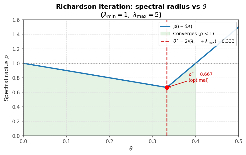

Richardson spectral radius ρ(I−θA) vs θ; optimal θ minimises the radius*

with corresponding optimal spectral radius

\[ \rho_{\mathrm{opt}} = \frac{\kappa_2(A) - 1}{\kappa_2(A) + 1}, \]

where \( \kappa_2(A) = \lambda_{\max}/\lambda_{\min} \) for a positive definite matrix. This reveals that convergence can be slow when the condition number is large, and that choosing the optimal \( \theta \) requires knowledge of (estimates of) the extreme eigenvalues.

31.2 Jacobi, Gauss-Seidel, and SOR Convergence

Theorem 31.2. If \( A \) and \( 2D - A \) are both SPD, then the Jacobi iteration converges.

Proof. Let \( \mu \) be an eigenvalue of \( G^J = I - D^{-1} A \). From the eigenvector equation, one derives \( v^T D v - v^T A v = \mu v^T D v \). Since \( A \) is SPD, \( v^T A v > 0 \), so \( (1-\mu) v^T D v > 0 \), giving \( \mu < 1 \). Since \( 2D - A \) is also SPD, a similar argument gives \( \mu > -1 \). Together, \( |\mu| < 1 \) for all eigenvalues, so \( \rho(G^J) < 1 \).

Theorem 31.3. If \( A \) is SPD, then Gauss-Seidel and SOR (for \( 0 < \omega < 2 \) both converge. For the special case of tridiagonal SPD matrices, the optimal SOR parameter is

\[ \omega_{\mathrm{opt}} = \frac{2}{1 + \sqrt{1 - \rho(G^J)^2}}. \]

Theorem 31.4. If \( A \) is an M-matrix (meaning \( a_{ii} > 0 \), \( a_{ij} \leq 0 \) for \( i \neq j \), and \( A^{-1} \) exists with non-negative entries), then both Jacobi and Gauss-Seidel converge, and Gauss-Seidel converges at least as fast as Jacobi: \( \rho(G^{\mathrm{GS}}) \leq \rho(G^J) < 1 \).

Stationary iteration methods tend to be slow at reducing low-frequency error components, since these correspond to eigenvalues near \( \lambda_{\min} \) where convergence is slowest. Their modern use is often as smoothers within multigrid methods, which exploit the fact that low-frequency components on a fine grid appear as higher-frequency components on coarser grids, enabling faster elimination by cycling between grid levels.

31.3 Convergence on the Discrete Poisson Equation

Analytical eigenvalue formulas allow precise convergence analysis on the familiar model problem. Consider the 2D Poisson equation \( -u_{xx} - u_{yy} = f \) (the negative sign ensures positive definiteness of the discrete matrix).

Theorem 31.5. For the negative of the 2D finite difference Laplacian with cell size \( h \) and \( m \) grid points per axis, the exact eigenvalues are

\[ \lambda_{ij} = \frac{4}{h^2} \left( \sin^2 \frac{\pi h i}{2} + \sin^2 \frac{\pi h j}{2} \right), \quad 1 \leq i, j \leq m. \]

The smallest eigenvalue is \( \lambda_{\min} = \frac{8}{h^2} \sin^2 \frac{\pi h}{2} \) and the largest is \( \lambda_{\max} = \frac{8}{h^2} \cos^2 \frac{\pi h}{2} \). The matrix is both SPD and an M-matrix, and its condition number worsens on finer grids. For example, with \( h = 1/10 \) (9 interior points per axis), \( \kappa_2 \approx 40 \), while with \( h = 1/100 \), \( \kappa_2 \approx 4000 \) — finer resolution leads to worse conditioning.

Richardson. The method converges for \( 0 < \theta < h^2/(4 \cos^2 \frac{\pi h}{2}) \), with optimal parameter \( \theta_{\mathrm{opt}} = 2/(\lambda_{\min} + \lambda_{\max}) \) giving

\[ \rho_{\mathrm{opt}} = 1 - 2 \sin^2 \frac{\pi h}{2}. \]

Jacobi. For the Poisson equation, the diagonal of \( A \) is \( D = (4/h^2) I \), which equals \( 1/\theta_{\mathrm{opt}} \). Therefore Jacobi iteration is equivalent to optimal Richardson for this problem, with

\[ \rho(G^J) = \cos(\pi h) = 1 - \frac{\pi^2 h^2}{2} + O(h^4). \]

For small \( h \) this is close to 1, indicating slow convergence.

Gauss-Seidel. Gauss-Seidel satisfies \( \rho(G^{\mathrm{GS}}) = [\rho(G^J)]^2 = \cos^2(\pi h) = 1 - \pi^2 h^2 + O(h^2) \). Gauss-Seidel converges exactly twice as fast as Jacobi, but this is only a constant factor improvement; for small \( h \) it remains slow.

SOR. With optimal \( \omega \),

\[ \omega_{\mathrm{opt}} = \frac{2}{1 + \sin(\pi h)}, \quad \rho_{\mathrm{opt}} = \omega_{\mathrm{opt}} - 1 = \frac{1 - \sin(\pi h)}{1 + \sin(\pi h)} = 1 - 2\pi h + O(h^2). \]

Optimal SOR is dramatically faster than the other stationary methods because its spectral radius depends on \( h \) rather than \( h^2 \). For \( h = 0.1 \), for example: \( \rho(G^J) \approx 0.95 \), \( \rho(G^{\mathrm{GS}}) \approx 0.90 \), \( \rho(G^{\mathrm{SOR}}) \approx 0.37 \).

---

Preconditioning

In this final lecture we examine the convergence of the conjugate gradient (CG) method in greater depth, then introduce preconditioning as a strategy to accelerate its convergence. The conjugate gradient method was introduced in Lecture 15.

32.1 Conjugate Gradient Convergence

At each step, CG finds the best solution \( x^{(k)} \) in the Krylov subspace \( \mathcal{K}_k(A) \), measured in the \( A \)-norm \( \|e\|_A = \sqrt{e^T A e} \). More precisely,

\[ \|e^{(k)}\|_A = \min_{x^{(0)} + x' \in \mathcal{K}_k(A)} \|x' - x\|_A. \]

Expanding the Krylov subspace in terms of the initial residual \( r^{(0)} = Ae^{(0)} \) and introducing a polynomial \( P_k(x) \) of degree at most \( k \) with \( P_k(0) = 1 \), we can write \( e^{(k)} = P_k(A) e^{(0)} \) and therefore

\[ \|e^{(k)}\|_A = \min \left\{ \|P_k(A) e^{(0)}\|_A : P_k \text{ polynomial of degree } \leq k,\ P_k(0) = 1 \right\}. \]

That is, CG implicitly finds the optimal degree-\( k \) polynomial to minimize the error. Using a specific Chebyshev-type polynomial to bound the error gives the following worst-case result.

Theorem 32.1.

\[ \|e^{(k)}\|_A \leq 2 \left( \frac{\sqrt{\kappa(A)} - 1}{\sqrt{\kappa(A)} + 1} \right)^k \|e^{(0)}\|_A. \]

The actual convergence often significantly exceeds this bound, depending on the full eigenvalue distribution. To see why, consider a matrix with only three distinct eigenvalues \( \lambda_1 < \lambda_2 < \lambda_3 \) (each possibly with multiplicity greater than one). We can construct a Lagrange polynomial \( P_3(x) \) of degree 3 such that \( P_3(0) = 1 \) and \( P_3(\lambda_j) = 0 \) for \( j = 1, 2, 3 \). Writing the initial error in terms of the eigenvectors of \( A \) and applying this polynomial, one finds

\[ \|e^{(3)}\|_A^2 = \sum_{j=1}^{n} \xi_j^2 [P_3(\lambda_j)]^2 \lambda_j = 0, \]

since each term vanishes. Therefore CG converges in exactly 3 iterations, regardless of \( \kappa(A) \). More generally, if \( A \) has \( m \) distinct eigenvalues, CG converges in at most \( m \) iterations. Clustering eigenvalues — rather than just minimizing the condition number — is the key to fast CG convergence, which motivates preconditioning.

32.2 Preconditioning Idea

Consider replacing the original system \( Ax = b \) with the equivalent system

\[ (M^{-1} A) x = M^{-1} b. \]

The matrix \( M \) is called the preconditioner. The solution is unchanged, but if \( M \) is chosen well, the modified system has a smaller condition number or more clustered eigenvalues, leading to faster CG convergence. Two requirements govern a good preconditioner: (1) \( M \approx A \), so that \( M^{-1} A \approx I \) and eigenvalues are clustered near 1; and (2) solves of the form \( Mz = c \) must be cheap, since a solve is required at each CG iteration.

Symmetric Preconditioning. CG requires the coefficient matrix to be SPD, but \( M^{-1} A \) is not symmetric in general even if \( M \) and \( A \) are. To restore symmetry, suppose \( M \) is SPD with Cholesky factorization \( M = LL^T \). Form the symmetrized system

\[ \underbrace{L^{-1} A L^{-T}}_{\tilde{A}} \underbrace{L^T x}_{\tilde{x}} = \underbrace{L^{-1} b}_{\tilde{b}}. \]

The matrix \( \tilde{A} = L^{-1} A L^{-T} \) is SPD by construction. Moreover, \( \tilde{A} \) and \( M^{-1} A \) have the same eigenvalues — one can verify this by observing that \( L^T (M^{-1} A) L^{-T} = \tilde{A} \) is a similarity transform. The naive implementation of this approach forms and solves the modified system explicitly, but this requires a full Cholesky factorization of \( M \) and may introduce significant fill.

32.3 Common Preconditioners

A better approach avoids forming \( \tilde{A} \) explicitly. Instead, one modifies the CG algorithm itself to incorporate the preconditioning step at each iteration. The preconditioned CG (PCG) algorithm adds a single solve \( z_k = M^{-1} r_k \) (or equivalently solves \( M z_k = r_k \) at each step; if \( M = I \), the standard CG algorithm is recovered.

Common preconditioners are related to the stationary iterative methods:

Jacobi preconditioning uses \( M_J = D \). This is the simplest possible preconditioner — just scaling each variable by the inverse of the corresponding diagonal entry — but it is often not very effective.

Symmetric Gauss-Seidel (SGS) uses \( M_{\mathrm{SGS}} = (D - L) D^{-1} (D - U) \). This can be factored as \( M_{\mathrm{SGS}} = L_M U_M \) where \( L_M = (D-L)D^{-1} \) and \( U_M = D - U \) are lower and upper triangular respectively. Solving \( M_{\mathrm{SGS}} z_k = r_k \) then requires only two triangular solves.

Symmetric SOR (SSOR) generalizes SGS with a relaxation parameter: \( M_{\mathrm{SSOR}} = (D - \omega L) D^{-1} (D - \omega U) \).

Incomplete Cholesky (IC) preconditioning builds a partial Cholesky factorization where \( LL^T \approx A \). A Cholesky-like process is applied to \( A \), but fill-in steps that would introduce new non-zero entries outside the sparsity pattern of \( A \) are skipped. The resulting \( L \) is sparse (its sparsity pattern stays close to \( A \)’s), so the cost of forming and applying the preconditioner remains low. The IC preconditioner is not guaranteed to exist in general, but it does exist for M-matrices and for the discrete Laplacian.

Sparsity of A, full Cholesky L, and incomplete Cholesky factor

The improvement in condition number from IC preconditioning can be dramatic. For the discrete Laplacian with \( m = 14 \) grid points per axis, the unpreconditioned system has \( \kappa(A) \approx 90.5 \) and requires 23 CG iterations to converge to tolerance \( 10^{-7} \). After IC preconditioning, the preconditioned system has \( \kappa(\tilde{A}) \approx 8.9 \) and requires only 14 PCG iterations — a substantial reduction in work.

32.4 Course Overview

This lecture concludes the course. The central themes running through CS475 were: the trade-off between direct and iterative methods; the role of matrix properties (sparsity, symmetry, definiteness, and rank) in the design and analysis of algorithms; the four major matrix factorizations — LU/Cholesky, QR, eigendecomposition, and SVD — and their applications to linear systems, least squares, and eigenvalue problems; and the fundamental importance of orthogonality throughout all of these topics.