CO 471/671: Semidefinite Optimization

These notes are based on Felix Zhou’s course notes. Additional explanations, visualizations, and examples have been added for clarity.

---

Semidefinite programming occupies a remarkable position in modern optimization. It sits strictly between linear programming and general convex optimization in expressive power, yet retains polynomial-time solvability. Its weapon is the positive semidefinite (PSD) cone: a closed convex cone with rich algebraic structure, a self-dual pairing, and a geometric shape that captures a breathtaking range of problems — from eigenvalue optimization to graph coloring bounds to polynomial nonnegativity certificates.

These notes trace the theory from first principles: the algebra of symmetric matrices, the geometry of the PSD cone, the primal–dual structure of semidefinite programs, the conditions guaranteeing strong duality, the algorithms that solve SDPs in polynomial time, and the applications that make SDP one of the most powerful tools in combinatorial and continuous optimization.

---

Chapter 1: Positive Semidefinite Matrices

Semidefinite programming is built on a single algebraic object: the cone of positive semidefinite matrices. Before studying optimization over this cone, we must understand its geometry, its characterizations, and the inner product that makes it self-dual. This chapter lays the algebraic foundation; everything else in the course is built on it.

1.1 Symmetric Matrices and the Trace Inner Product

\[ \mathcal{S}^n := \{X \in \mathbb{R}^{n \times n} : X^T = X\}. \]

This is a vector space of dimension \(\frac{n(n+1)}{2}\), and it carries a natural inner product. To perform linear programming over matrix spaces, we need a notion of “dot product” for matrices; the trace inner product is the right choice.

The dimension count \(\frac{n(n+1)}{2}\) is not merely an abstract fact — it corresponds to an explicit coordinatization of \(\mathcal{S}^n\). The map \(\mathrm{s2vec}\) makes this concrete by flattening a symmetric matrix into a vector in the right way.

\[ \langle X, Y \rangle_{\mathrm{trace}} = \mathrm{s2vec}(X)^T \mathrm{s2vec}(Y) \quad \text{for all } X, Y \in \mathcal{S}^n. \]

In particular, \(\mathrm{s2vec}\) is a bijection, and its inverse \(\mathrm{mat2vec} = \mathrm{s2vec}^{-1}\) reconstructs \(X\) from its coordinate vector by placing each entry back and dividing off-diagonal entries by \(\sqrt{2}\). This coordinatization is useful when one wants to write an SDP in LP-like form with explicit variable vectors — for instance, in analyzing the structure of the feasible set or in certain interior-point implementations.

The trace inner product makes \(\mathcal{S}^n\) a Hilbert space — a complete inner product space — of dimension \(\frac{n(n+1)}{2}\). All the standard tools of linear programming (dual cones, separating hyperplanes, complementary slackness) generalize to this setting via this inner product.

The trace is invariant under cyclic permutation: \(\operatorname{Tr}(ABC) = \operatorname{Tr}(CAB) = \operatorname{Tr}(BCA)\). This elementary fact is used constantly in proofs.

Every \(X \in \mathcal{S}^n\) has an eigenvalue decomposition. Since \(X\) is symmetric, its eigenvalues are real; we order them \(\lambda_1(X) \geq \lambda_2(X) \geq \cdots \geq \lambda_n(X)\). The spectral theorem is the key structural result that allows us to “diagonalize” the analysis of symmetric matrices.

The spectral decomposition says that every symmetric matrix is, up to rotation, just a diagonal matrix. This diagonalization is what allows us to reduce many properties of symmetric matrices — including positive semidefiniteness — to conditions on their eigenvalues.

1.2 Positive Semidefinite Matrices

With the spectral decomposition in hand, we can now define the central object of the course: positive semidefinite matrices. Geometrically, a PSD matrix is one whose associated quadratic form is everywhere nonnegative — it “curves upward” in all directions.

The condition \(h^T X h \geq 0\) for all \(h\) is a nonnegativity condition on the quadratic form associated with \(X\). It is the matrix analogue of the scalar condition \(x \geq 0\), and just as \(\mathbb{R}_+\) is the “nonnegative orthant” in scalar LP, \(\mathcal{S}^n_+\) is the “nonnegative cone” in SDP.

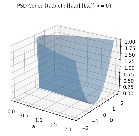
The PSD cone \(\mathcal{S}^n_+\) is a proper closed convex cone: it is closed under non-negative linear combinations and its only lineality is \(\{0\}\). For \(2 \times 2\) matrices, the condition \(\begin{bmatrix}a & b \\ b & c\end{bmatrix} \succeq 0\) is equivalent to \(a \geq 0\), \(c \geq 0\), and \(ac \geq b^2\) — a solid cone in the \((a,b,c)\) space as shown above.

The following theorem gives five equivalent ways to recognize a PSD matrix, each illuminating a different aspect of the concept.

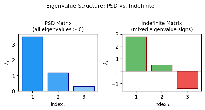
Characterization (2) is particularly vivid: a symmetric matrix is PSD precisely when its eigenvalues are all nonneg­ative. Characterization (3) links PSD to Gram matrices of vectors — a bridge that is essential for SDP relaxations of combinatorial problems, since it allows us to interpret a PSD matrix as a collection of vectors in \(\mathbb{R}^n\). Characterization (5) says that \((\mathcal{S}^n_+)^* = \mathcal{S}^n_+\), making it a self-dual cone — the same cone appears on both sides of the duality pairing.

The Cholesky decomposition is the computational workhorse for checking PSD-ness: it runs in \(O(n^3)\) time and either produces a triangular factor \(B\) (confirming PSD-ness) or fails at a zero or negative pivot (certifying non-PSD). Moreover, \(\mathcal{S}^n_{++} = \operatorname{int}(\mathcal{S}^n_+)\): the positive definite matrices are the interior of the PSD cone.

1.3 The Schur Complement Lemma

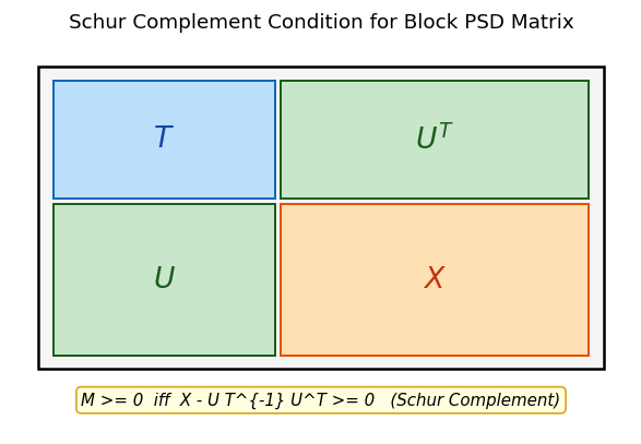
A key tool for converting nonlinear constraints into linear matrix inequalities (LMIs) is the Schur complement condition. Many constraints of the form “matrix \(X\) dominates product \(UV^T\)” can be lifted into a linear block-matrix inequality, opening the door to SDP formulations.

The Schur complement \(X - UT^{-1}U^T\) is the matrix analogue of the scalar expression \(c - ba^{-1}b\) appearing in \(2 \times 2\) Gaussian elimination. It measures how much of \(X\) “remains” after accounting for the contribution from the \(T\)-block through the off-diagonal \(U\).

The proof is an instance of the general principle that block Gaussian elimination — a purely algebraic operation — preserves definiteness. The nonsingularity of \(L\) is essential: it ensures that the change of variables does not destroy the PSD condition.

A special case (\(m=1, T=1\)) gives: \(\begin{bmatrix} 1 & x^T \\ x & X \end{bmatrix} \succeq 0 \iff X - xx^T \succeq 0\). This is the SDP-based reformulation of the constraint “\(X\) dominates \(xx^T\)” — foundational for lifting vector quadratics into SDPs.

1.4 Complementarity

In LP, the complementary slackness conditions \(x_j s_j = 0\) characterize optimal primal-dual pairs. In SDP, the analogous condition involves the trace inner product and the matrix product. Understanding this condition is essential for both the theory of strong duality and the design of interior-point methods.

The proof uses the symmetrized form \(X^{1/2} S X^{1/2}\) — a standard technique in matrix analysis that “symmetrizes” a product while preserving its eigenvalues up to sign. The key step is that a PSD matrix with zero trace must be the zero matrix.

This result plays the role for SDPs that \(x_j \cdot s_j = 0\) plays for LP: it is the complementary slackness condition characterizing optimal pairs. In geometric terms, \(XS = 0\) means that the column spaces of \(X\) and \(S\) are orthogonal — the primal and dual solutions “live on complementary faces” of the PSD cone.

---

Chapter 2: Semidefinite Programs

With the algebraic foundation in place, we can now define the main object of the course: the semidefinite program. An SDP is to LP as the PSD cone is to the nonneg­ative orthant — everything is the same except we replace the scalar nonnegativity constraint \(x \geq 0\) with the matrix PSD constraint \(X \succeq 0\). This single change dramatically increases the expressive power of the problem class while retaining polynomial-time solvability.

2.1 Standard Form

Recall that a linear program optimizes a linear function subject to linear constraints. A semidefinite program (SDP) optimizes a linear function of a matrix variable subject to linear (affine) constraints and a PSD constraint. The linear objective \(\langle C, X \rangle = \operatorname{Tr}(CX)\) is the natural generalization of \(c^T x\) to the matrix setting.

\[ (P) \quad \inf_{X \in \mathcal{S}^n} \langle C, X \rangle \quad \text{s.t.} \quad \mathcal{A}(X) = b, \quad X \succeq 0. \]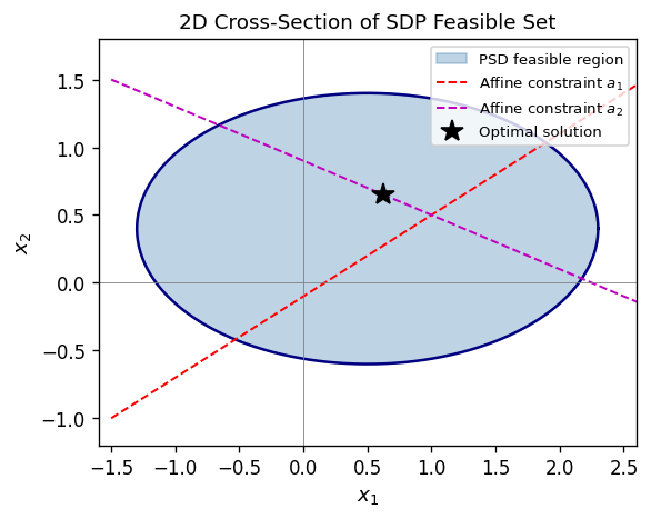

The feasible set is the intersection of the PSD cone with an affine subspace — a spectrahedron. It is convex by construction. The objective \(\langle C, X \rangle = \operatorname{Tr}(CX)\) is linear in \(X\), so the problem is convex. Being a convex optimization problem, it has no spurious local minima; any local optimum is global.

Why SDPs? The PSD constraint \(X \succeq 0\) is highly nonlinear (in the original matrix entries), yet computationally tractable. It allows one to encode, for instance, the constraint that a Gram matrix \(X = V^T V\) represents unit vectors with prescribed inner products — the foundation for relaxing combinatorial problems like MAX-CUT. The PSD constraint captures a richer family of feasible sets than linear constraints, and this extra expressive power is what gives SDPs their approximation power for hard combinatorial problems.

2.2 The SDP Dual

\[ \langle \mathcal{A}^*(y), X \rangle = \langle y, \mathcal{A}(X) \rangle \quad \forall X \in \mathcal{S}^n, y \in \mathbb{R}^m, \]\[ (D) \quad \sup_{y \in \mathbb{R}^m, S \in \mathcal{S}^n} b^T y \quad \text{s.t.} \quad \mathcal{A}^*(y) + S = C, \quad S \succeq 0. \]

The dual variable \(S \succeq 0\) acts as a slack in the dual constraint: feasibility of \((D)\) means \(C - \mathcal{A}^*(y) \succeq 0\). The dual of \((D)\) is equivalent to \((P)\), so SDP duality is an involution — the dual of the dual is the primal, exactly as in LP.

2.3 Weak Duality

Weak duality is the first and most fundamental consequence of the SDP primal-dual structure: any feasible primal value is an upper bound on any feasible dual value. This allows feasible dual solutions to certify the quality of primal solutions.

The proof is a clean algebraic manipulation using the adjoint relationship and primal feasibility. The key step is expanding \(\langle C, \bar{X} \rangle\) using the dual constraint \(C = \mathcal{A}^*(\bar{y}) + \bar{S}\) and then using the adjoint identity.

Consequences: if \((P)\) is unbounded below, then \((D)\) is infeasible; if \((D)\) is unbounded above, then \((P)\) is infeasible. If \(\langle \bar{X}, \bar{S} \rangle = 0\) for some feasible pair, then both are optimal.

2.4 Certifying Infeasibility

In LP, the Farkas lemma gives a complete characterization of infeasibility via a dual certificate. In SDP, the situation is more delicate: there is no exact analogue, and infeasibility can be “almost feasible” in a way that has no LP counterpart.

The SDP analogue of Farkas’ lemma is more subtle — there is no exact analogue. However:

The concept of almost feasibility is uniquely SDP: unlike LP, infeasibility and near-infeasibility can differ. This is one of the genuine pitfalls of semidefinite programming. The gap between infeasibility and almost-feasibility is precisely what the Slater condition (Chapter 3) is designed to exclude. The formal definition:

Note that feasibility implies almost feasibility. The two theorems that characterize almost feasibility give a precise description of when the dual constraint system is genuinely infeasible versus merely pathologically close to feasibility.

Together, Theorems 2.2.1 and 2.2.2 give a complete characterization: the system \(\mathcal{A}^*(y) \preceq C\) is either almost feasible or admits an explicit certificate of “true” infeasibility in the form of a matrix \(D \succeq 0\) with \(\mathcal{A}(D) = 0\) and \(\operatorname{Tr}(CD) < 0\).

---

Chapter 3: Duality Theory

Chapter 2 introduced the SDP primal-dual pair and established weak duality. The deeper question — when does the duality gap vanish? when do both problems attain their optima? — is the subject of this chapter. The answers are more subtle than in LP: strong duality does not always hold for SDPs, and understanding when it fails motivates the Slater condition and the facial reduction algorithm.

3.1 Conic Duality Framework

\[ (P): \inf \langle c, x \rangle,\ \mathcal{A}(x) = b,\ x \in K \qquad (D): \sup \langle b, y \rangle + \langle d, u \rangle,\ \mathcal{A}^*(y) + \mathcal{B}^*(u) + s = c,\ u \geq 0,\ s \in K^*. \]

The following definitions formalize the two key cones used in duality. The dual cone captures all vectors that have nonneg­ative inner product with every element of \(K\) — the conic analogue of a “dual feasible direction.”

The self-duality of \(\mathcal{S}^n_+\) — the fact that \(K^* = K\) — is what makes SDP duality so symmetric and elegant. It is the reason the same cone appears in both the primal and dual problems.

A closely related object is the polar set, which generalizes duality to non-conic convex sets.

Observe that if \(K\) is a cone, then \(K^o = -K^*\). The polar set is always closed and convex regardless of the structure of \(K\).

The Legendre-Fenchel conjugate is the key tool that relates primal and dual objective functions in conic optimization, and in particular connects the log-barrier for SDPs to its dual form.

A fundamental example, which appears in the analysis of interior-point methods, is the log-determinant barrier.

This conjugate pair underlies the self-concordance of the log-barrier and the derivation of the dual barrier in interior-point methods.

3.2 The Slater Condition

The Slater condition is the regularity condition that guarantees strong duality in SDP. In LP, mere feasibility of both primal and dual suffices for strong duality; in SDP, one needs strict interior feasibility — a Slater point.

Slater points — strictly interior feasible solutions — are the regularity condition that tames duality gaps in SDP. Under LP, feasibility alone suffices; under SDP, one needs strict interior feasibility. The Slater condition is not just a technical convenience: without it, SDPs can exhibit pathological behavior (duality gaps, non-attainment) that never occurs in LP.

---

Chapter 4: Strong Duality, Slater Condition, and Facial Reduction

We now develop the conditions under which the duality gap vanishes and optimal values are attained. The key theorem — strong duality under the Slater condition — is the SDP analogue of LP’s fundamental theorem of linear programming. We also study what goes wrong when the Slater condition fails and how facial reduction can restore it.

The proof of strong duality rests on the following fundamental results from convex analysis, which we state explicitly.

These separation results are the backbone of the proof of strong duality: the Slater point ensures that the interior of the PSD cone intersects the dual feasible region, which makes the two convex sets \(G_1\) and \(G_2\) in the proof disjoint and allows separation.

4.1 Strong Duality

The strong duality theorem says that, when the dual has a Slater point and is bounded, the primal optimum exists and equals the dual supremum. This is the essential tool for certifying SDP optimality: finding a feasible dual solution with value \(z^*\) proves that no primal solution can do better.

The proof uses hyperplane separation in matrix space: the Slater point for the dual ensures that the interior of \(\mathcal{S}^n_+\) is nonempty and intersects the dual feasible region, enabling separation from the set of dual solutions that achieve or exceed \(z^*\).

The corollary covers the most common case in applications: both primal and dual have strictly feasible points, so strong duality holds and both optima are attained.

4.2 Pitfalls Without Slater Points

Unlike LP, SDPs can exhibit pathological behavior when Slater points are absent:

1. Duality gap: Even with both primal and dual feasible and bounded, the optimal values of \((P)\) and \((D)\) may differ.
2. Non-attainment: The infimum in \((P)\) (or supremum in \((D)\)) may not be achieved.
3. Strict complementarity may fail: Even with Slater points, there may be no optimal pair \(\bar{X}, (\bar{y}, \bar{S})\) satisfying \(\bar{X} + \bar{S} \succ 0\) (rank complementarity). Compare with LP, where strict complementarity always holds.

In LP, feasibility of both primal and dual guarantees attainment. In SDP, only Slater’s condition (strict interior feasibility) provides this guarantee. These pathologies — duality gaps and non-attainment — are genuine obstacles in practice and motivate the facial reduction approach of Section 4.3.

4.3 Faces of the PSD Cone and Facial Reduction

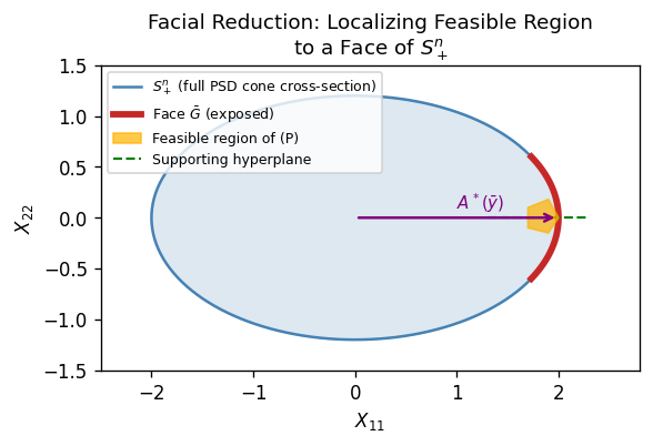
When the Slater condition fails, the feasible region of the SDP lies on a face of the PSD cone — a lower-dimensional subset. By identifying this face and restricting the problem to it, we can restore the Slater condition and guarantee strong duality. This is the idea behind facial reduction.

Faces of a cone are the “boundary strata” of the cone — the subsets where the cone “touches” a supporting hyperplane. For the PSD cone, faces are characterized by rank constraints on the null space.

The structure theorem is elegant: faces of the PSD cone are parametrized by subspaces, and each face is itself a smaller PSD cone. This recursive structure is what makes facial reduction an iterative, finite process.

Every proper face of \(\mathcal{S}^n_+\) is linearly isomorphic to \(\mathcal{S}^k_+\) for some \(k < n\). This means the feasible region of \((P)\) lives in a smaller cone \(\mathcal{S}^k_+\), and replacing \((P)\) by an equivalent SDP over \(\mathcal{S}^k_+\) can restore the Slater condition.

Facial Reduction Algorithm. Given that \((P)\) lacks a Slater point, find \(\bar{y}\) such that \(\mathcal{A}^*(\bar{y}) \in \mathcal{S}^n_+ \setminus \{0\}\) with \(b^T \bar{y} = 0\). The hyperplane \(\{X : \langle X, \mathcal{A}^*(\bar{y}) \rangle = 0\}\) is a supporting hyperplane of \(\mathcal{S}^n_+\) containing the feasible region, exposing a proper face. By iterating at most \(n\) times, we arrive at an SDP over \(\mathcal{S}^k_+\) that necessarily satisfies the Slater condition (by minimality of the face). This is facial reduction. Each iteration reduces the dimension of the cone by at least one, so the process terminates in at most \(n\) steps.

The dichotomy lemma is the key that drives facial reduction: at every stage, either the Slater condition holds (and we are done) or there is a facial reduction direction that strictly reduces the dimension. The two alternatives are mutually exclusive and exhaustive.

4.4 Extended Lagrange-Slater Dual

When facial reduction is not applied and the Slater condition fails, one can instead pass to an extended dual that repairs the attainment failure at the cost of a larger problem. This is the Extended Lagrange-Slater Dual.

\[ (\text{ELSD}): \inf \operatorname{Tr}(C(U+W)),\quad \mathcal{A}(U+W) = b,\quad W \in \mathcal{W}^n,\quad U \succeq 0, \]

where \(\mathcal{W}^n \subseteq \mathcal{S}^n\) is a linear subspace determined by \(\mathcal{A}\) and \(C\).

The ELSD thus “fixes” attainment when the primal lacks a Slater point, at the cost of enlarging the problem. It is a theoretical device rather than a practical algorithm — in practice, facial reduction is the preferred approach.

Two additional results describe when the Slater condition holds in the SDP relaxations that arise from combinatorial optimization problems.

This is a powerful representational result: it means that essentially any constraint set arising from polynomial optimization can be lifted into the SDP framework. The construction reduces polynomial constraints to quadratic ones using auxiliary variables.

Thus the Slater condition can always be guaranteed in SDP relaxations of polynomial optimization problems, provided the convex hull of the feasible set has been correctly identified (or we can work in the correct affine subspace).

---

Chapter 5: Solving SDPs

Having established the duality theory, we now turn to algorithms. How does one actually compute the optimal solution to an SDP? Two paradigms are developed: the ellipsoid method, which is polynomial for any convex program with an efficient separation oracle, and primal-dual interior-point methods, which are the practical workhorse of SDP solvers. SDPs can be solved in polynomial time by two main algorithmic paradigms: the ellipsoid method (theoretically important, polynomial in all inputs) and primal-dual interior-point methods (practically efficient with \(O(\sqrt{n})\) iterations).

5.1 The Ellipsoid Method

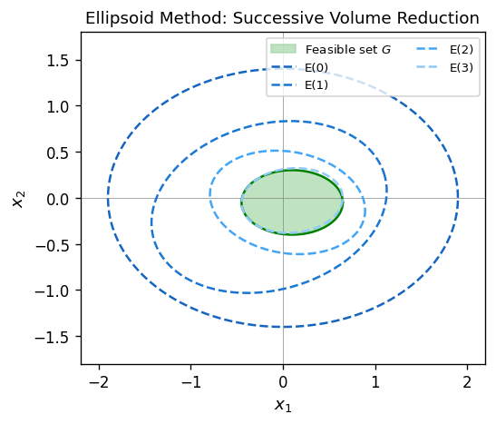
The ellipsoid method is the first polynomial-time algorithm for convex optimization, and in particular for SDP. It works by maintaining an ellipsoid enclosing the feasible set and repeatedly halving its volume using separating hyperplanes. The key requirement is a separation oracle — an algorithm that, given any point, either confirms feasibility or produces a separating hyperplane.

Ellipsoids are the natural “balls” in the geometry of the algorithm: the shape matrix \(A\) encodes the eccentricity of the ellipsoid, and the center \(c\) is the current best guess for a feasible point. A foundational result ensures that every compact convex set with nonempty interior is approximated well by an ellipsoid.

The Löwner-John theorem is the foundation for the volume argument in the ellipsoid method and also underlies the John ellipsoid theory used in convex geometry and algorithm design.

What makes the ellipsoid method genuinely revolutionary — and what earned Khachiyan the Fulkerson Prize — is that it does not require an explicit description of the feasible region at all. You don’t need to write down all the constraints; you only need a separation oracle: a black-box subroutine that, given any point, either certifies that it is feasible or produces a hyperplane separating it from the feasible set. This oracle model is extraordinarily powerful. For SDPs, the separation oracle for the PSD cone is just checking whether a symmetric matrix has a negative eigenvalue — an \(O(n^3)\) computation. For combinatorial polyhedra like the matching polytope, the separation oracle is a min-cut computation. The ellipsoid method thus reduces polynomial-time optimization to polynomial-time separation, a profound insight that predates interior-point methods by a decade and remains theoretically fundamental.

The ellipsoid method does not require an explicit description of the feasible region; it only needs a weak separation oracle. We formalize the relevant notions.

In each iteration, the new minimum-volume ellipsoid containing the feasible half of the current ellipsoid satisfies an explicit update formula with guaranteed volume reduction.

This lemma gives the explicit per-iteration volume reduction of at least \(e^{-1/(2d)}\), which yields the polynomial iteration bound.

The volume reduction per iteration — at least a \((1 - 1/(2d))\) fraction — is the key bound. The total number of iterations is polynomial in the dimension and the logarithm of the precision, giving a polynomial-time algorithm.

For optimization, one additionally needs a subgradient oracle for the objective. The following theorem makes this precise.

\[ (\tilde{P}): \quad \inf \langle C, X \rangle,\quad \mathcal{A}(X) = b,\quad \langle \bar{S}, X \rangle \leq 2\langle \bar{X}, \bar{S} \rangle,\quad X \succeq 0. \]

Theorem 3.1.4 ensures that the modified SDP has a compact feasible set with explicit inner and outer ball bounds, making it directly amenable to Theorem 3.1.3 and hence solvable by the ellipsoid method.

5.2 Primal-Dual Interior-Point Methods

The ellipsoid method is polynomially efficient in theory but slow in practice. Interior-point methods, by contrast, are the basis of all modern SDP solvers and run in \(O(\sqrt{n})\) iterations. They work by staying strictly inside the PSD cone and following a curved path — the central path — toward the optimum.

Interior-point methods generate sequences \((X^{(k)}, y^{(k)}, S^{(k)})\) with \(X^{(k)}, S^{(k)} \succ 0\), maintaining primal and dual feasibility while driving the duality gap \(\langle X^{(k)}, S^{(k)} \rangle \to 0\).

\[ f(X) := -\ln \det X, \quad X \in \mathcal{S}^n_{++}, \]

with gradient \(f'(X)[H] = -\operatorname{Tr}(X^{-1}H)\) and Hessian \(f''(X)[H,H] = \operatorname{Tr}(X^{-1}HX^{-1}H)\). This function blows up at the boundary of the PSD cone, naturally enforcing \(X \succ 0\). The log-determinant barrier is the canonical self-concordant barrier for the PSD cone. The formal statement of its derivatives and strict convexity is:

These derivative formulas are the starting point for Newton’s method on the barrier-penalized problem and for computing the search directions in interior-point algorithms.

5.3 The Central Path

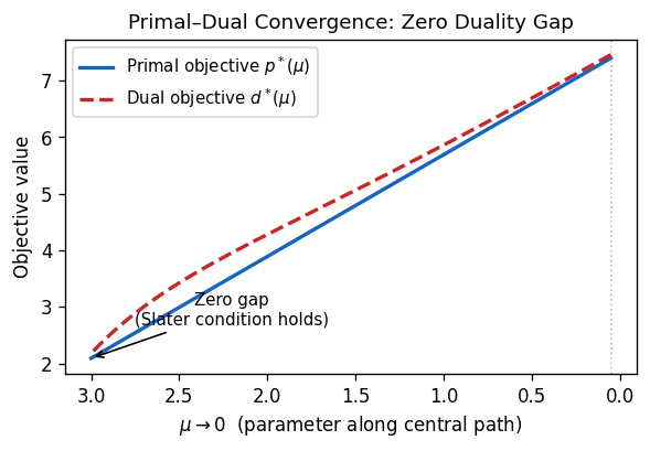
The central path is a one-parameter family of strictly feasible primal-dual pairs, parameterized by the barrier parameter \(\mu > 0\). As \(\mu \to 0\), the central path converges to the optimal solution. Interior-point algorithms follow this path approximately, taking Newton steps to stay close.

\[ (P_\mu): \quad \inf \frac{1}{\mu}\langle C, X \rangle - \ln \det X, \quad \mathcal{A}(X) = b. \]\[ \mathcal{A}(X) = b, \quad X \succ 0, \quad \mathcal{A}^*(y) + S = C, \quad S = \mu X^{-1}. \]

The uniqueness of the central path solution is a consequence of strict convexity of the barrier-penalized problem. The formal statement is:

The duality gap \(\langle X(\mu), S(\mu) \rangle = n\mu\) decreases linearly with \(\mu\), so driving \(\mu \to 0\) drives the gap to zero and recovers the optimal solution in the limit.

5.4 Path-Following and Potential Reduction

The central path gives a theoretical route to the optimum, but following it exactly requires solving nonlinear systems at each step. Practical interior-point methods instead follow the path approximately, using a potential function to measure “closeness to the central path” and taking steps that reduce this potential.

\[ \psi(X, S) := n \ln \frac{\operatorname{Tr}(XS)}{n} + f(X) + f(S) = n \ln \frac{\operatorname{Tr}(XS)}{n} - \ln \det X - \ln \det S. \]

The nonnegativity of \(\psi\) follows from the AM-GM inequality applied to the eigenvalues of \(S^{1/2}XS^{1/2}\): the arithmetic mean of eigenvalues is at least the geometric mean. Equality in AM-GM forces all eigenvalues to be equal, which is precisely the central path condition \(S = \mu X^{-1}\).

\[ \phi_\rho(X, S) := \rho \ln \langle X, S \rangle + \psi(X, S), \quad \rho > 0. \]

Search direction. To achieve the potential decrease required by Theorem 3.2.4, one exploits a scaling automorphism of the PSD cone.

In the \(V\)-space induced by this scaling, the search direction that maximally reduces the duality gap is the projection of \(-V\) onto the feasible subspace. The following lemma bounds the barrier function change along a search direction.

The condition \(\|D\|_X \leq 1\) is equivalent to \(X \pm D \succeq 0\), i.e., \(X+D\) remains positive definite. The upper bound is the self-concordance estimate for the log-determinant barrier.

The \(O(\sqrt{n})\) iteration bound is a hallmark of SDP interior-point methods — it is analogous to the \(O(\sqrt{m})\) bound for LP interior-point methods and arises from the self-concordance of the log-determinant barrier.

\[ (P_{\text{aux}}): \quad \inf\, \xi \quad \text{s.t.} \quad \mathcal{A}(X) + \xi(b - \mathcal{A}(I)) = b,\ \langle I, X \rangle \leq M,\ \xi \geq 0,\ X \succeq 0, \]

for which \((X^{(0)}, \xi_0) = (I, 1)\) is a Slater point.

Computational remarks. For LP, data of bit-length \(L\) ensures rational optima and bounds \(\gamma \approx 2^{-L}, M \approx 2^L\). For SDP, even with binary data, the optimal solution may be irrational, and the bounds can be doubly exponential in \(L\). SDP feasibility is in NP and co-NP in the real-number model; whether it is in P (in the Turing machine model) remains open.

---

Chapter 6: Applications

With the theory firmly in hand — the algebra of PSD matrices, the duality of SDPs, the algorithms that solve them in polynomial time — we turn to the applications that have made semidefinite programming one of the most influential developments in modern optimization. The applications in this chapter are not minor improvements over existing methods; they represent genuine breakthroughs, each solving a problem that had resisted purely combinatorial or LP-based approaches.

The unifying theme is that the PSD constraint encodes geometric structure that LP cannot capture. By allowing the optimization variable to be a matrix rather than a vector, we gain the ability to encode dot products, angles, and dependencies between variables — the language of Euclidean geometry. This extra expressive power is exactly what is needed to resolve deep questions in graph theory, information theory, and algebraic geometry.

The final chapter demonstrates the breadth and power of semidefinite programming through a selection of landmark applications. We see SDP as an approximation tool for NP-hard combinatorial problems (MAX-CUT and the Goemans-Williamson algorithm), as a bound on information-theoretic quantities (the Lovász theta function and Shannon capacity), as a framework for lifting combinatorial relaxations (lift-and-project methods), and as the foundation for polynomial optimization (sum-of-squares hierarchies). Each application reveals a different facet of the SDP paradigm.

6.1 MAX-CUT via Goemans-Williamson

The MAX-CUT problem is one of the most celebrated applications of SDP: a semidefinite relaxation combined with random hyperplane rounding gives a \(0.878\)-approximation, far better than what is achievable by purely combinatorial methods.

Problem. Given an undirected graph \(G = (V, E)\) with edge weights \(w \in \mathbb{R}^E_+\), find \(U \subseteq V\) maximizing \(\sum_{ij \in \delta(U)} w_{ij}\).

\[ \max_{u \in \{-1,1\}^n} \frac{1}{4} \sum_{i,j} w_{ij}(1 - u_i u_j). \]\[ \max \tfrac{1}{4}\bigl(\langle W, \mathbf{1}\mathbf{1}^T \rangle - \langle W, X \rangle\bigr) \quad \text{s.t.} \quad \operatorname{diag}(X) = \mathbf{1},\quad X \succeq 0,\quad \operatorname{rank}(X) = 1. \]\[ (\text{SDP}): \quad \max -\tfrac{1}{4}\operatorname{Tr}(WX) + \tfrac{1}{4}\mathbf{1}^T W \mathbf{1} \quad \text{s.t.} \quad \operatorname{diag}(X) = \mathbf{1},\quad X \succeq 0. \]

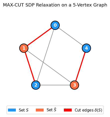
Goemans-Williamson random hyperplane rounding. Given an optimal solution \(\hat{X} = BB^T\) with columns \(v^{(1)}, \ldots, v^{(n)}\) (unit vectors), pick \(r\) uniformly on the unit sphere and set \(U = \{i : r^T v^{(i)} \geq 0\}\). The hyperplane through the origin with normal \(r\) partitions the unit vectors — and hence the vertices — into two sides.

The key inequality in the proof is made precise by the following two lemmas from Felix’s notes:

Together these two lemmas give the expected cut value. The final theorem makes the polynomial-time statement precise.

This approximation ratio \(\rho \approx 0.878\) is optimal assuming the Unique Games Conjecture (Khot-Vishnoi). It represents a fundamental barrier: no polynomial-time algorithm can do significantly better unless NP-hard problems can be solved in polynomial time.

The Goemans-Williamson result is a watershed in the history of approximation algorithms. Before 1995, the best known approximation for MAX-CUT was \(1/2\) (achieved by a trivial random algorithm). The SDP relaxation — a natural lifting of the \(\{-1,+1\}\) constraint to unit vectors — combined with the random hyperplane argument gave an immediate jump to \(0.878\). The fact that this ratio is conditionally optimal (assuming the Unique Games Conjecture) means the SDP analysis is not an artifact of the proof technique but reflects genuine structural information. The random hyperplane rounding step, meanwhile, is a master key: the same idea, applied to different SDP relaxations, unlocks approximation algorithms for dozens of other combinatorial problems.

6.2 Maximum Satisfiability and Quadratic Optimization

The Goemans-Williamson technique extends to Maximum Satisfiability problems. The following NP-hardness result places the approximation results in context.

Max 2-SAT is closely related to MaxCut: given a MaxCut instance on \(G\) with unit edge weights, one can construct a Max 2-SAT instance with \(\mathrm{OPT}(\text{Max 2-SAT}) = \mathrm{OPT}(\text{MaxCut}) + 2|E|\), so approximation results for MaxCut yield analogous results for Max 2-SAT.

\[ \bar{f}(W) := \max_{x \in \{-1,1\}^n} x^T W x, \quad f(W) := \min_{x \in \{-1,1\}^n} x^T W x, \]\[ \bar{F}(W) := \max\{\operatorname{Tr}(WX) : \operatorname{diag}(X) = \mathbf{1},\, X \succeq 0\}, \quad F(W) := \min\{\operatorname{Tr}(WX) : \operatorname{diag}(X) = \mathbf{1},\, X \succeq 0\}. \]

The two lemmas below convert the optimization over sign vectors into an expectation over random hyperplanes and then into a transformed SDP via the arcsin function.

The case \(W \in \mathcal{S}^n_+\) includes all MaxCut instances (the Laplacian of any graph with nonneg­ative weights is PSD by the Gershgorin Disk Theorem). For general \(W\):

The bound \(\frac{2}{\pi}\) in the PSD case is sharp — achievable by specific instances — and the \((\frac{2}{\pi})^2\) bound for the general case is likewise tight. The key identity is \(\bar{f}(W) = \frac{2}{\pi} \max\{\langle W, \arcsin(X) \rangle : \operatorname{diag}(X) = \mathbf{1},\, X \succeq 0\}\), connecting the nonconvex problem to a transformed SDP via the arcsine function.

6.3 Geometric Representation of Graphs

The preceding two sections showed SDP at work on optimization problems — MAX-CUT, MAX-SAT — where we relax a hard combinatorial objective and round a continuous solution back to an integer one. We now shift perspective entirely. In this section and the next, SDP is not a relaxation tool but an exact characterization tool. We ask: what is the information-theoretic capacity of a graph? And can we compute it in polynomial time? The answer, through the Lovász theta function, is a resounding yes — using SDP.

Here we arrive at one of the most beautiful chapters in all of combinatorial optimization. The story begins with a deceptively simple question: can we represent the structure of a graph using Euclidean geometry? More precisely, if we assign vectors to vertices, what constraints does the edge structure impose on those vectors? The answer, developed through the theory of orthonormal representations, is the key that unlocks the Lovász theta function — one of the most celebrated results at the intersection of information theory, combinatorics, and semidefinite programming.

The idea is to move from the combinatorial world of vertices and edges to the continuous world of vectors in \(\mathbb{R}^d\). Non-edges between vertices in \(G\) become orthogonality conditions on the corresponding vectors. This translation — combinatorial structure into geometric language — is precisely what makes SDP so powerful for graph problems: the PSD constraint exactly captures the space of all valid Gram matrices of such vector systems.

The theory of geometric representations is the foundation for everything that follows. Crucially, this theory is not just a curiosity — it is what makes the Lovász theta function computable. Because the set of all valid Gram matrices of a vector assignment is exactly the PSD cone, every question about orthonormal representations becomes an SDP feasibility or optimization question. Geometry and algebra lock together perfectly.

Before studying the Lovász theta function, we need the theory of geometric representations of graphs, which is Felix’s Chapter 5. This theory connects graph structure to Euclidean geometry via SDP and provides the crucial notion of orthonormal representations used in the theta body.

The proof embeds \(K_n\) as the vertices of a regular simplex in \(\mathbb{R}^{n-1}\) where all edges have unit length; any graph on \(V\) is a subgraph of \(K_n\). The existential result is easy; the real difficulty — and the motivation for SDP — is minimizing the dimension of such a representation, which leads to the hard problem of Theorem 5.1.2.

The NP-hardness of computing the minimum embedding dimension (Theorem 5.1.2) means we cannot efficiently minimize the dimension of unit-distance representations. This is a recurring theme: the combinatorial question is hard, but a continuous relaxation — via SDP — is tractable. Rather than optimizing over the dimension, one can find the minimum enclosing ball of a unit-distance representation via SDP. Let \(t_b(G)\) denote the square of the minimum radius of a ball containing some unit-distance representation of \(G\).

One can also find the minimum enclosing hypersphere (sphere, not ball). Let \(t_h(G)\) be the square of its radius.

This bound on the radius is tight for complete graphs and ensures all unit-distance hypersphere representations are bounded.

The radius bound \(t_b(G) < 1/2\) (Corollary 5.1.4.1) is not just a technical detail — it is the exact threshold needed to convert between two dual geometric languages: unit-distance representations of a graph and orthonormal representations of its complement. This bijection is what makes the complement operation so natural in this theory.

Orthonormal representations. Unit-distance representations on a hypersphere with \(t < 1/2\) correspond bijectively to orthonormal representations of the complement graph.

The key correspondence is: a unit-distance hypersphere representation of \(G\) with radius \(\sqrt{t}\) (\(t < 1/2\)) gives an orthonormal representation of \(\bar{G}\) by rescaling; conversely, an orthonormal representation of \(G\) gives a unit-distance hypersphere representation of \(\bar{G}\). This duality between \(G\) and its complement \(\bar{G}\) is central to the Lovász theory. When you assign orthonormal vectors to the vertices of \(G\) such that non-adjacent vertices get orthogonal vectors, you are encoding the structure of \(G\) in the angles between vectors — a language that SDP reads naturally through the Gram matrix.

Notice the elegant interplay: geometry on \(G\) corresponds to geometry on \(\bar{G}\). This complement-duality will reappear at the heart of the theta function theory, where the SDP for \(\theta(G)\) and the SDP for \(\theta(\bar{G})\) are in exact primal-dual correspondence. The SDP duality theorem becomes, in graph-theoretic language, a statement about the relationship between independence numbers and chromatic numbers.

6.4 The Lovász Theta Function

The Lovász theta function is one of the most elegant applications of SDP to graph theory. It provides a polynomial-time computable bound on both the independence number and the chromatic number of a graph, sandwiching between two NP-hard quantities. Its connection to the Shannon capacity of a graph is one of the deepest results in information theory and combinatorics.

\[ \alpha(G) \leq \theta(G) \leq \chi(\bar{G}). \]

On the left sits the independence number \(\alpha(G)\) — the size of the largest independent set, an NP-hard quantity in general. On the right sits the chromatic number of the complement \(\chi(\bar{G})\) — also NP-hard. Sandwiched between them is \(\theta(G)\), computable in polynomial time via SDP. This is not merely a curiosity: the theta function is computable while the quantities it bounds are not.

The historical context is equally striking. In 1979, László Lovász was studying the Shannon capacity of the five-cycle \(C_5\). The five-cycle models a noisy communication channel where each symbol can be confused with its two neighbors; the capacity measures how many distinct messages can be sent without possibility of confusion. It was known that \(\alpha(C_5) = 2\) (two non-adjacent vertices) and \(\alpha(C_5^{\otimes 2}) = 5\) (five non-adjacent vertices in the strong square), so the capacity is at least \(\sqrt{5}\). But could it be higher? The question had been open for years. Lovász introduced \(\theta(G)\) precisely to resolve it: he proved \(\theta(C_5) = \sqrt{5}\), and since \(\theta\) upper-bounds the Shannon capacity, the capacity is exactly \(\sqrt{5}\). A decades-old open problem, resolved in a single paper using what is now recognized as semidefinite programming. The elegance and power of this approach transformed the field.

What Lovász realized — and this is the key insight — is that the geometric language of orthonormal representations is exactly the right language for bounding the independence number. An independent set in \(G\) corresponds to a clique in \(\bar{G}\), and a clique in \(\bar{G}\) corresponds to a set of vertices that are mutually adjacent, i.e., pairwise non-orthogonal in an orthonormal representation of \(G\). By optimizing over all such representations simultaneously using SDP, one obtains a bound that is computable in polynomial time yet captures information that purely LP-based methods cannot access.

\[ \text{FRAC}(G) := \{x \in [0,1]^V : x_i + x_j \leq 1 \text{ for all } ij \in E\}. \]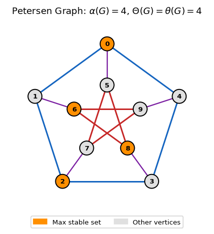

The theta body interpolates between them. It is a semidefinitely-defined polytope that is computable in polynomial time and provides a tighter relaxation of STAB(\(G\)) than the naive LP relaxation.

The sandwich theorem says that the theta body sits between two NP-hard polytopes, providing a polynomial-time computable approximation to both. For perfect graphs, these four polytopes coincide — a characterization that leads directly to the Strong Perfect Graph Theorem. The fact that \(\mathrm{TH}(G)\) is sandwiched between \(\mathrm{STAB}(G)\) (the convex hull of integer solutions) and \(\mathrm{CLQ}(G)\) (a natural LP relaxation) is precisely what makes it such a powerful tool: it is simultaneously a valid relaxation for stability and an approximation for clique-number bounds, all achievable in polynomial time.

The theta body \(\mathrm{TH}(G)\) is the single most elegant object in this course. It is defined geometrically — through orthonormal representations — yet it is an SDP-feasible set, making it computable in polynomial time. It is simultaneously a relaxation of the integer programming polytope \(\mathrm{STAB}(G)\) and a tighter relaxation than the naive LP relaxation \(\mathrm{FRAC}(G)\). No purely LP-based approach can achieve this sandwiching; the SDP structure is essential.

Given \(w \in \mathbb{R}^V_+\), the Lovász theta function is \(\theta(G, w) := \max_{x \in \mathrm{TH}(G)} w^T x\). Setting \(w = \mathbf{1}\) gives \(\theta(G) := \theta(G, \mathbf{1})\). This function is computable by SDP.

The theorem shows that \(\theta(G,w)\) is efficiently computable by SDP (items 3 and 4 are SDPs). The four equivalent formulations are remarkable: the first is geometric (optimal orthonormal representation with handle), the second is a minimax over geometric configurations, and the third and fourth are clean semidefinite programs. The primal SDP (item 4) maximizes over PSD matrices with zero entries on edges; the dual SDP (item 3) minimizes over a spectral condition. Strong duality of SDP connects these two seemingly different formulations. The four equivalent formulations in Theorem 5.2.3 are not just mathematically elegant — they are computationally crucial. Formulations (3) and (4) are semidefinite programs that can be solved by any standard SDP solver. Formulation (2) gives the geometric interpretation: \(\theta(G,w)\) is the inverse square of the smallest “handle” needed to “catch” any feasible orthonormal representation weighted by \(w\). The primal-dual relationship between formulations (3) and (4) is precisely the strong duality of SDP, and it gives, for free, the sandwich inequality \(\alpha(G) \leq \theta(G) \leq \chi(\bar{G})\): the independence number is a lower bound because any independent set gives a feasible dual solution, and the chromatic number of \(\bar G\) is an upper bound because any proper coloring of \(\bar G\) gives a feasible primal solution.

The following two definitions are needed for the perfect graph characterization.

A perfect graph is one that behaves as “nicely as possible” from a coloring standpoint: in every induced subgraph, the chromatic number equals the clique number, so there is no “waste” in the coloring. Perfect graphs include bipartite graphs, chordal graphs, interval graphs, and comparability graphs — large, well-structured families. For these graphs, many NP-hard problems (stable set, coloring, clique cover) become polynomial, a consequence of the Ellipsoid Method and the Lovász theta function.

Perfect graphs are an extraordinary class. The definition — \(\omega(H) = \chi(H)\) for every induced subgraph \(H\) — says that the chromatic number never “wastes” colors: you always need exactly as many colors as the largest clique forces you to use. This property holds for bipartite graphs (no odd cycles at all), chordal graphs (every cycle has a chord), interval graphs, and comparability graphs of partial orders. For all these classes, the theta body \(\mathrm{TH}(G)\) collapses to the integer hull \(\mathrm{STAB}(G)\), meaning the SDP relaxation is already tight — no rounding is needed. This gives polynomial-time algorithms for stable set, coloring, and clique-cover on perfect graphs, via the Ellipsoid Method applied to the theta body.

The Strong Perfect Graph Theorem (item 3 in the equivalence above) deserves special attention. Claude Berge conjectured in 1960 that a graph is perfect if and only if it contains no odd hole (chordless odd cycle of length \(\geq 5\)) and no odd antihole (complement of an odd hole). The conjecture was immediately plausible — odd holes are the simplest “imperfect” configurations — but a proof eluded researchers for over 40 years. The eventual proof by Chudnovsky, Robertson, Seymour, and Thomas in 2006 required over 150 pages and introduced entirely new graph-theoretic techniques. It stands as one of the great theorems of modern combinatorics. The connection to SDP is through item 5: a graph is perfect if and only if \(\mathrm{STAB}(G) = \mathrm{TH}(G)\), so the SDP relaxation is already exact on perfect graphs. This means the LP relaxation of the stable set problem has an exact SDP witness — the theta body — on all perfect graphs, enabling polynomial-time optimization over the stable set polytope.

It is worth pausing to appreciate the depth of the Perfect Graph Theorem. The equivalence of items 1 through 8 connects graph structure (no odd holes/antiholes), polyhedral geometry (four polytopes coinciding), SDP (the theta body is a polytope), and total dual integrality (the clique constraint system is TDI). These are different languages for the same truth, unified by the Lovász theta function and SDP duality.

The theta body has a natural dual description in terms of the complement graph.

The polar relationship \([\mathrm{TH}(G)]^o \cap \mathbb{R}^V_+ = \mathrm{TH}(\bar{G})\) is the geometric expression of a deep duality: the theta bodies of complementary graphs are polar to each other. In SDP terms, this is exactly SDP strong duality — the primal SDP for \(\theta(G)\) and the dual SDP for \(\theta(\bar{G})\) are each other’s dual problems. The geometric and algebraic dualities coincide perfectly.

Before connecting the Lovász theta to channel capacity, we recall the strong product. The strong product models simultaneous use of a channel: if \(G\) is the confusion graph of a single channel use, then \(G^k\) is the confusion graph of \(k\) simultaneous uses. Two codewords of length \(k\) can be confused if, in every coordinate, the symbols are either identical or confusable in the single-use graph. The capacity — the asymptotic rate of distinguishable messages — is the Shannon capacity \(\Theta(G)\).

The Shannon capacity models the maximum rate of error-free communication over a noisy channel whose confusion graph is \(G\). To understand the definition: if symbols \(i\) and \(j\) are connected in \(G\) (they can be confused), then transmitting codewords of length \(k\) corresponds to using the strong product \(G^k\). The independence number \(\alpha(G^k)\) counts the maximum number of distinguishable codewords of length \(k\). The Shannon capacity \(\Theta(G) = \lim_{k\to\infty} \alpha(G^k)^{1/k}\) is the asymptotic rate of growth — the channel capacity in Shannon’s sense. Computing \(\Theta(G)\) exactly is open in general, which is why the Lovász upper bound is so valuable: it provides a computable upper bound via SDP.

The multiplicativity \(\theta(G \otimes H) = \theta(G)\cdot\theta(H)\) is the key structural property that makes \(\theta\) an upper bound on the Shannon capacity. The proof uses Kronecker products: if \(\{v_i\}\) is an orthonormal representation of \(G\) with unit handle \(c\), and \(\{u_j\}\) is one for \(H\) with unit handle \(d\), then \(\{v_i \otimes u_j\}\) is an orthonormal representation of \(G\otimes H\) with handle \(c \otimes d\). The product of optimal values follows from the product of inner products. This is a beautiful example of the tensor product method, where higher-dimensional algebra (Kronecker products) proves statements about graph products.

The multiplicativity of \(\theta\) under the strong product — \(\theta(G \otimes H) = \theta(G)\cdot\theta(H)\) — is the key property that makes it an upper bound on the Shannon capacity: it grows at the right rate under repetition. The analogous multiplicativity of \(\alpha\) is unknown in general, and this is precisely why computing \(\Theta(G)\) is hard. The theta function “interpolates” between \(\alpha\) (which fails multiplicativity) and \(\chi(\bar{G})\) (which is also multiplicative) in a way that is simultaneously computable and a valid bound. The proof of multiplicativity uses a beautiful construction: if \(v_1, \ldots, v_{|V|}\) is an orthonormal representation of \(G\) with handle \(c_G\), and \(u_1, \ldots, u_{|W|}\) is one for \(H\) with handle \(c_H\), then the Kronecker products \(v_i \otimes u_j\) with handle \(c_G \otimes c_H\) give an orthonormal representation of \(G \otimes H\). The product of the optimal values follows algebraically.

For the Petersen graph, \(\alpha = 4\) and \(\theta = 4\), confirming \(\Theta(\text{Petersen}) = 4\) — a result that eluded direct combinatorial proof for years. The SDP-based proof is short and clean; the purely combinatorial proof remained out of reach for decades. Similarly, for \(C_5\), Lovász proved \(\theta(C_5) = \sqrt{5}\), so \(\alpha(C_5) = 2 \leq \Theta(C_5) \leq \theta(C_5) = \sqrt{5}\). Since \(\alpha(C_5^{\otimes 2}) = 5\) (from the five-coloring of \(C_5^{\otimes 2})\), we get \(\Theta(C_5) \geq \sqrt{5}\), and combined with the upper bound, \(\Theta(C_5) = \sqrt{5}\). The irrational capacity of the pentagon channel is an exact answer from a polynomial-time SDP computation — one of the most striking applications of optimization to information theory ever found.

Perfect graphs. For perfect graphs, the inequality chain \(\alpha(G) \leq \Theta(G) \leq \theta(G) \leq \chi(\bar{G})\) collapses to equality, giving a complete description of the stable set polytope via clique inequalities. This is not a coincidence: perfectness is precisely the condition under which the theta body, the stable set polytope, and the clique polytope all coincide, and the SDP is automatically an exact formulation of the integer program.

6.5 Lift-and-Project Methods

The Goemans-Williamson relaxation lifts a combinatorial problem into a semidefinite program and then “rounds” the SDP solution back to an integer solution. The lift-and-project framework formalizes this idea into a systematic hierarchy of increasingly tight relaxations. Starting from a weak LP relaxation of an integer program, each application of the \(\mathrm{LS}_+\) operator lifts to a higher-dimensional spectrahedron and projects back, tightening the relaxation.

The central challenge of integer programming is that LP relaxations are often far too weak: the LP optimum can be a fractional point far from any integer solution. The idea behind lift-and-project is to “lift” the problem into a higher-dimensional space — adding new variables that capture products of the original variables — solve an SDP in this lifted space, and then project back. The projection is a strictly tighter relaxation of the original integer program. By repeating this operation, we construct a hierarchy of relaxations that converges, in a finite number of steps, to the exact integer hull.

The \(\mathrm{LS}_+\) operator (Lovász-Schrijver with PSD constraints) is particularly powerful because it can simultaneously enforce many types of valid inequalities — odd-cycle inequalities, odd-antihole inequalities, odd-wheel inequalities — that would require exponentially many cutting planes to encode individually. A single application of \(\mathrm{LS}_+\) to the fractional stable set polytope \(\mathrm{FRAC}(G)\) recovers all these inequalities at once, illustrating that semidefinite lifting is a fundamentally more powerful operation than LP-based cutting.

To understand the lifting, think of what happens when we have a fractional solution \(x \in P \setminus P_I\) — a point that is “almost integer” but not quite. An LP relaxation cannot distinguish this from an integer point because it only knows linear functions of \(x\). To cut it off, we need to reason about products of the original variables: knowing that \(x_i \cdot x_j\) must equal \(x_i\) or \(0\) (since \(x_i, x_j \in \{0,1\}\)) is a quadratic constraint that LPs cannot encode but SDPs can. The lift-and-project framework introduces matrix variables \(Y_{ij}\) representing these products, imposes PSD constraints (so the lifted matrix is a valid “moment matrix”), and then projects back onto the original space. The projection is tighter than the original polytope because the SDP constraints capture the integrality structure more faithfully.

\[ \mathrm{LS}_+(P) := \{x \in \mathbb{R}^d : \exists Y \in M_+(K),\ (1, x)^T = Y e_0\}, \]

where \(M_+(K)\) is the PSD-feasible region of a lifted system encoding \(Y e_i \in K\) and \(Y(e_0 - e_i) \in K\) for all \(i\), and \(K\) is the homogenization of \(P\).

The finite convergence after \(d\) rounds is the key result: the \(\mathrm{LS}_+\) hierarchy always reaches the integer hull in finitely many steps, though the number of steps required can be as large as \(d\) (the number of variables). The inclusion of the theta body in the first round shows that a single application of \(\mathrm{LS}_+\) is already more powerful than the LP relaxation. This is remarkable: the theta body — which took Lovász deep geometric insight to define — emerges naturally from a single mechanical application of the \(\mathrm{LS}_+\) operator. It suggests that the theta body is, in some precise sense, the “right” first-level SDP relaxation for stable set problems.

The hierarchy structure also has practical implications. If you need to solve a hard combinatorial optimization problem and have limited computational budget, you can choose the level \(k\) of the hierarchy as a trade-off between tightness (higher \(k\) gives a tighter relaxation) and computational cost (the SDP grows with \(k\)). This explicit parameterization of the quality-complexity trade-off is one of the key advantages of the lift-and-project framework over ad hoc cutting plane methods.

Applied to \(\mathrm{FRAC}(G)\), a single application of \(\mathrm{LS}_+\) recovers odd-cycle, odd-antihole, and odd-wheel inequalities simultaneously — a remarkable unification of combinatorial cutting plane methods via SDP. Each of these families of valid inequalities was discovered independently in the graph theory literature, typically requiring problem-specific combinatorial arguments to derive. The \(\mathrm{LS}_+\) operator produces all of them in one shot, with no combinatorial case analysis required. This is the power of the SDP lifting: it finds valid inequalities that are invisible to LP-based methods.

The \(\mathrm{LS}_+\) construction can be generalized far beyond \(\{0,1\}\) polytopes. Any compact set — including non-polyhedral sets arising from continuous optimization with polynomial constraints — can be tightened using the same lifting idea. The Successive Convex Relaxation Method (SCRM) is the general framework, and the theorems below show that \(\mathrm{LS}_+\) is a special case. This unification is important: it means the same algorithmic and theoretical tools apply to integer programs, polynomial optimization, and constraint satisfaction problems with polynomial structure.

Theorem 6.3.5 shows that the \(\mathrm{LS}_+\) hierarchy is a special case of the SCRM: iterating SCRM with the integrality constraints is precisely the same as applying \(\mathrm{LS}_+\) repeatedly. This unifies the two approaches. In practice, one never iterates all the way to the integer hull — the \(d\)-th level SDP is as large as the original problem — but the hierarchy provides a rigorous framework for understanding the gap between fractional and integer optimal values. The rate at which this gap closes across levels of the hierarchy is a measure of the “integrality gap” of the LP relaxation, and it is a topic of active research in theoretical computer science.

6.6 Sum-of-Squares and Polynomial Optimization

We have now seen SDP applied to graph theory (via the Lovász theta function) and to integer programming (via lift-and-project). The third great application domain is polynomial optimization: minimizing a polynomial \(p_0(x)\) subject to polynomial constraints \(p_i(x) \geq 0\). This class is extraordinarily broad — it includes linear programming (\(d = 1\)), quadratic programming (\(d = 2\)), and NP-hard combinatorial problems that can be encoded as polynomial feasibility questions.

The challenge is that polynomial nonnegativity is, in general, undecidable (Hilbert’s tenth problem). But there is a computable sufficient condition for nonnegativity: being a sum of squares. A polynomial \(f\) is a sum of squares (SOS) if \(f = \sum_i g_i^2\) for some polynomials \(g_i\). Every SOS polynomial is nonneg­ative, and the question of whether \(f\) is SOS is exactly an SDP feasibility problem — just check whether the Gram matrix \(X\) satisfying \(f(x) = h(x)^T X h(x)\) can be chosen PSD. This transforms a question in real algebraic geometry into a linear algebra problem over the PSD cone.

The deep result — Stengle’s Positivstellensatz — says that this SOS approach is not just sufficient but, for bounded feasible sets, also asymptotically necessary: if \(f \geq 0\) on the feasible set, then for large enough degree, there is an SOS certificate. This completeness is what turns SOS into a systematic hierarchy of SDP relaxations, not just a one-off trick.

The final application brings SDP to bear on polynomial optimization — a class of problems that generalizes both LP and SDP. A polynomial that is nonneg­ative everywhere can be certified as such by expressing it as a sum of squares; checking this certificate is an SDP. This idea leads to a hierarchy of SDP relaxations for polynomial optimization that converges to the exact optimum.

Let us make this SDP reduction precise. Given a polynomial \(f : \mathbb{R}^n \to \mathbb{R}\) of degree \(2d\), let \(h(x) \in \mathbb{R}^N\) be the vector of monomials of degree \(\leq d\) (with \(N = \binom{n+d}{d}\)), and define \(\mathcal{F}(f) := \{X \in \mathcal{S}^N : h(x)^T X h(x) = f(x)\}\). Then \(f\) is a sum of squares (SOS) iff \(\mathcal{F}(f) \cap \mathcal{S}^N_+ \neq \emptyset\), which is an SDP feasibility problem.

This SDP-based characterization of SOS polynomials is the key bridge between real algebraic geometry and semidefinite programming. For each degree bound \(d\), one solves a single SDP of size \(N = \binom{n+d}{d}\). As \(d\) increases, the SDP grows but the relaxation tightens, giving the Lasserre hierarchy of SDP relaxations for polynomial optimization. The hierarchy below captures this precisely.

\[ \inf_{x \in \mathbb{R}^n} p_0(x) \quad \text{s.t.} \quad p_1(x) \geq 0, \ldots, p_m(x) \geq 0. \]

Theorem 7.2.1 is the Real Positivstellensatz, and it is one of the deepest results in real algebraic geometry. It says that infeasibility of a polynomial system has an algebraic certificate in the form of SOS polynomials. The degree of the certificate — the smallest \(d\) for which such \(s_J\) exist — can be large, but it is always finite. In practice, one increases \(d\) until the SDP is feasible; if the system is infeasible, this terminates in finite time with a certificate. If the system is feasible, the SDP becomes feasible at some level as well, giving an approximate solution of increasing accuracy.

This is a generalization of both Farkas’ lemma (for linear feasibility) and Hilbert’s Nullstellensatz (for polynomial equations over \(\mathbb{C}\)). The following classical result is the complex analogue.

Over the complex numbers, the algebra is “nicer” — the Nullstellensatz is exact with no SOS needed, and the certificate is just a linear combination of the generators. Over the real numbers, one needs the SOS multipliers to handle positivity rather than just zero-sets, and this is precisely where SDP enters. The SOS certificates are the “real analogue” of the complex algebraic certificates, and they are checkable by SDP rather than by algebra alone.

For each degree bound \(d\), one solves an SDP whose feasibility certifies positivity of \(p_0\) on the feasible set. By Theorem 7.2.1 (Stengle’s Positivstellensatz), the hierarchy is complete: for sufficiently large \(d\), the SOS certificate exists whenever \(p_0 \geq 0\) on the feasible set. This completeness is what makes SOS hierarchies a rigorous approach rather than a heuristic.

The connection to integer programming is direct: the constraints \(x_i \in \{0,1\}\) can be written as \(x_i^2 - x_i = 0\), and maximizing a linear objective over the \(0\)–\(1\) cube is a polynomial optimization problem. The SOS hierarchy applied to this formulation recovers the \(\mathrm{LS}_+\) hierarchy of the previous section — another example of the deep unity between seemingly different SDP frameworks. The SOS framework also connects to control theory (certifying stability of nonlinear dynamical systems via Lyapunov functions) and statistics (bounding moments of random variables via moment matrices). Its reach extends far beyond combinatorics.

6.7 Extension Complexity

We close the course with what may be the most surprising and beautiful result: extension complexity. The question is fundamental. We know that LP can be solved in polynomial time, and SDPs can too. But does this mean that any problem for which a polynomial-time algorithm exists must have a compact LP or SDP formulation? The answer — made precise by Yannakakis in 1988 — is a resounding no, and the proof is algebraic.

The question of extension complexity is: given a polytope \(P\) (say, the convex hull of all tours of a TSP instance, or of all matchings in a graph), what is the smallest LP that can represent it? More precisely: what is the minimum number of inequalities in any higher-dimensional polyhedron \(Q\) that projects down to \(P\)? If this number is polynomial, then LP-based algorithms can solve the problem efficiently. If it is exponential, no compact LP can solve it — we would need exponentially many constraints, defeating the purpose.

Yannakakis’s theorem gives a precise algebraic answer: the minimum size of any LP extension of \(P\) equals the nonneg­ative rank of the slack matrix of \(P\). The slack matrix encodes, in a single matrix, all the slack values of all extreme points in all facet inequalities. The nonneg­ative rank of this matrix is therefore the bottleneck: if it is large, no compact LP exists.

The implications are profound. Rothvoß proved in 2017 that the TSP polytope and the matching polytope both have exponential extension complexity — their slack matrices have exponential nonneg­ative rank. This means there is provably no compact LP that can solve the Traveling Salesman Problem or the Matching Problem exactly, unless P = NP (and even then the LP would be exponential in size). For matching, this is particularly striking: the problem is polynomial-time solvable (Edmonds’ algorithm), but there is no compact LP formulation. The polynomial-time algorithm works for a different reason — a combinatorial argument — not because of a small LP description.

Let us make these ideas precise. Given a polytope \(P \subseteq \mathbb{R}^d\) with \(m\) facets and \(n\) extreme points, the slack matrix \(S \in \mathbb{R}^{m \times n}_+\) has \(S_{ij} = b_i - \langle a^{(i)}, v^{(j)} \rangle\). The nonneg­ative rank \(\mathrm{rank}_+(S)\) is the smallest \(k\) for which \(S = FV^T\) with \(F \in \mathbb{R}^{m \times k}_+\), \(V \in \mathbb{R}^{n \times k}_+\), and we set \(\mathrm{rank}_+(P) := \mathrm{rank}_+(S)\).

Yannakakis’ theorem gives a clean algebraic characterization of the minimum size of any LP extension: it is exactly the nonneg­ative rank of the slack matrix. This result — proved in 1988 and published in 1991 — launched the field of extension complexity and ultimately led to exponential lower bounds for the TSP polytope, dashing hopes for a compact LP formulation of the traveling salesman problem. The key algebraic insight is that an LP extension of \(P\) is equivalent to a nonneg­ative factorization of the slack matrix: each row of the factorization corresponds to a constraint in the extension, and each column corresponds to an extreme point. The nonneg­ative rank measures exactly how many “atoms” are needed in this factorization.

To understand the theorem intuitively: every facet inequality \(a_i^T x \leq b_i\) of the extension, when evaluated at the extreme points \(v_j\) of \(P\), gives a nonneg­ative slack. The slack matrix \(S_{ij} = b_i - a_i^T v_j\) can be written as a product of two nonneg­ative matrices if the extension has a compact LP form. If the nonneg­ative rank of \(S\) is large, no such compact factorization exists, and hence no compact LP extension exists.

The polytope case is complete: Yannakakis’ theorem fully characterizes LP extension complexity. The natural next question is: what about SDP extensions? Can a polytope with exponential LP extension complexity have a polynomial SDP extension complexity? The answer is yes, and the theory of semidefinite extension complexity — developed by Gouveia, Parrilo, and Thomas — provides the framework. The generalization to convex sets uses a slack function. For a compact convex set \(G\) with \(0 \in \mathrm{int}(G)\), the slack function is \(S_G : \mathrm{ext}(G) \times \mathrm{ext}(G^\circ) \to \mathbb{R}\) given by \(S_G(x, s) := 1 - \langle x, s\rangle\). A \(K\)-factorization of \(S_G\) is a pair of maps \(V : \mathrm{ext}(G) \to K\) and \(F : \mathrm{ext}(G^\circ) \to K^*\) such that \(S_G(x,s) = \langle V(x), F(s)\rangle\) for all \((x,s)\).

Setting \(K = \mathcal{S}^n_+\) (so \(K^* = K\)) gives the SDP extension complexity framework: a convex set \(G\) has a lifted \(\mathcal{S}^n_+\)-representation if and only if the slack function has a \(\mathcal{S}^n_+\)-factorization. This SDP generalization opens the door to “SDP extension complexity” — a rich theory connecting the geometry of polytopes to the algebra of PSD matrices, and providing a unified framework for the lift-and-project methods of Section 6.5.

The Gouveia-Parrilo-Thomas theorem thus completes the picture: LP extension complexity is controlled by nonneg­ative rank of the slack matrix, while SDP extension complexity is controlled by the PSD rank (the smallest \(r\) for which the slack function has a PSD-factorization with \(r \times r\) PSD matrices). Every polytope with a polynomial SDP extension complexity can be optimized over by a polynomial-size SDP — and the lift-and-project methods of Section 6.5 are exactly the algorithmic tools for constructing such extensions. Conversely, if the PSD rank is exponential, no polynomial-size SDP can represent the polytope, and one must resort to exponential-time methods.

This is where the course ends: at the frontier of what SDP can and cannot do. Semidefinite programming is extraordinarily powerful — it captures orthonormal representations, Lovász theta functions, polynomial nonnegativity certificates, and lifted integer programming relaxations — but it is not all-powerful. The theory of extension complexity provides the ultimate limitation: some polytopes are inherently compact, some require large SDPs, and some even resist exponential-size LPs. Understanding these boundaries is the central challenge of modern optimization theory, and the tools developed in this course — PSD matrices, duality theory, interior-point methods, orthonormal representations, and the Positivstellensatz — are the foundation on which that understanding is built.

---

For further reading: Vandenberghe and Boyd, “Semidefinite Programming,” SIAM Review 38(1), 1996; Lovász, “On the Shannon Capacity of a Graph,” IEEE Trans. Inf. Theory 25(1), 1979; Goemans and Williamson, “Improved Approximation Algorithms for MAX-CUT and MAX-SAT,” JACM 42(6), 1995.