Sources and References

Primary textbook — Schroeder, D. V. An Introduction to Thermal Physics. Addison-Wesley, 2000.

Supplementary texts — Pathria, R. K. and Beale, P. D. Statistical Mechanics, 4th ed. Academic Press, 2021; Kardar, M. Statistical Physics of Particles. Cambridge University Press, 2007; Reif, F. Fundamentals of Statistical and Thermal Physics. McGraw-Hill, 1965; Kittel, C. and Kroemer, H. Thermal Physics, 2nd ed. W. H. Freeman, 1980; Sethna, J. P. Statistical Mechanics: Entropy, Order Parameters, and Complexity, 2nd ed. Oxford University Press, 2021; Huang, K. Statistical Mechanics, 2nd ed. Wiley, 1987.

Online resources — Tong, D. Statistical Physics (Cambridge Part II Mathematical Tripos lecture notes); MIT OpenCourseWare 8.044 Statistical Physics I and 8.333 Statistical Mechanics I (Kardar); NIST Chemistry WebBook.

---

Part I: Foundations and the Three Ensembles

Chapter 1: The Statistical Programme

Why big is different

Every physics course you have encountered before statistical mechanics considers a narrow slice of nature: the electric field of a point charge, the trajectory of a projectile, the propagation of a wave through a uniform medium. You are trained to track individual particles and solve equations of motion for each of them. Statistical mechanics is radically different. Its subject is systems with so many degrees of freedom that tracking individuals is not only impractical but, more surprisingly, unnecessary. The three-body gravitational problem is already intractable in general; a three-body interaction in a fluid, similarly, admits no clean analytic solution. Yet when you have \(10^{23}\) molecules, the physics becomes simpler, not harder. That apparent paradox is the central message of this chapter.

The reason is that we change our question. Instead of asking “what is the position and momentum of molecule number 4,183,771?” we ask “what is the pressure of this gas? What is its temperature? How much heat will it absorb if we raise the temperature by ten degrees?” These macroscopic questions are statistical questions — answers that sum over the enormous multiplicity of microscopic configurations. The theory that does this systematically is statistical mechanics, and it has turned out to be one of the most broadly applicable frameworks in all of science, reaching from astrophysics (neutron stars) to condensed matter (superconductors) to biology (protein folding) and even economics (agent-based models of markets).

Equilibrium and the fundamental postulate

Before we can count anything, we need an assumption powerful enough to make the statistics well-defined. Statistical mechanics rests on a single foundational principle, stated here in the careful language of Schroeder:

In an isolated system at equilibrium, all accessible microstates are equally probable.

An equilibrium state is one in which all macroscopic variables — pressure, volume, temperature, magnetisation — have ceased to change with time. This does not mean that nothing is happening at the microscopic level. Gas molecules are still bouncing off walls; electrons are still hopping between orbitals. Equilibrium is a macroscopic concept, meaning that the aggregate statistics of these microscopic processes have stabilised. A gas in a cylinder with a fixed piston is in mechanical equilibrium: the average force the gas exerts on the piston equals the external pressure, even though individual molecules hit the piston at random times. A chemical system at equilibrium has fixed concentrations, even though individual molecules continue to react in both directions. A system in thermal equilibrium exchanges energy with its surroundings at the same rate in both directions, so the net energy flow is zero.

The word isolated is equally important. An isolated system cannot exchange energy or particles with anything outside itself. Its total energy \(E\), volume \(V\), and particle number \(N\) are all fixed. In practice we often relax one or more of these constraints — allowing energy exchange with a heat bath, or particle exchange with a particle reservoir — and that relaxation gives rise to the canonical and grand canonical ensembles we will develop in later chapters. But the fundamental postulate applies to the isolated case, and everything else is built from it.

Given equal probability of all microstates, the central task of statistical mechanics is counting: how many microstates \(\Omega\) are compatible with the observed macroscopic state? A state with more microstates will be overwhelmingly more likely to be observed than one with few microstates. This shifts the whole enterprise from dynamics to combinatorics.

Combinatorics: the mathematics of counting

Two counting techniques appear throughout this course, and you should have seen both in PHYS 358.

Combinations. When we have \(N\) distinguishable objects and wish to choose \(k\) of them (without regard to order), the number of ways to do so is the binomial coefficient

\[ \binom{N}{k} = \frac{N!}{k!\,(N-k)!}. \]

The canonical physics example is a spin-\(\tfrac{1}{2}\) paramagnet: \(N\) independent magnetic dipoles, each pointing either up or down. If \(N_\uparrow\) of them point up, the number of distinct spin configurations with that value of \(N_\uparrow\) is \(\Omega = \binom{N}{N_\uparrow}\). Note the symmetry \(\binom{N}{k} = \binom{N}{N-k}\): the number of ways to have \(N_\uparrow\) up-spins equals the number of ways to have \(N - N_\uparrow\) down-spins, which is physically obvious — you are just relabelling up and down.

Ball-and-stick counting (stars and bars). The second technique addresses the question: in how many ways can \(q\) identical balls be distributed among \(N\) bins? Represent the \(N\) bins by the \(N-1\) dividers between them; then arrange the \(q\) balls and \(N-1\) sticks in a row. Any ordering of these \(q + N - 1\) objects corresponds to a valid distribution, and the number of such orderings is

\[ \Omega = \binom{q + N - 1}{q}. \]

For an Einstein solid — \(N\) quantum harmonic oscillators sharing \(q\) units of vibrational energy — the oscillators are the bins and the energy quanta are the balls. The number of accessible microstates with total energy \(E = q\hbar\omega\) is therefore \(\Omega = \binom{N+q-1}{q}\). This simple formula encapsulates the entire statistical mechanics of the Einstein solid.

Stirling’s approximation and why statistical mechanics works

Almost every application of these counting formulae involves factorials of astronomically large numbers. If \(N \sim N_A \approx 6 \times 10^{23}\), computing \(N!\) directly is hopeless. Stirling’s approximation rescues us:

\[ N! \approx N^N e^{-N} \sqrt{2\pi N}, \qquad \ln N! \approx N\ln N - N + \tfrac{1}{2}\ln N. \]

For the sizes of \(N\) we encounter, the \(\tfrac{1}{2}\ln N\) term is negligible compared to \(N\ln N\), so the working approximation is simply \(\ln N! \approx N\ln N - N\).

The derivation of Stirling’s formula is itself instructive. We begin with the gamma function representation of the factorial. By successive integration by parts, one can verify that

\[ N! = \Gamma(N+1) = \int_0^\infty t^N e^{-t}\,dt. \]

The integrand \(t^N e^{-t}\) vanishes at both endpoints and has a single maximum. To find the maximum, write the integrand as \(e^{N\ln t - t}\) and differentiate the exponent with respect to \(t\), setting the result to zero:

\[ \frac{d}{dt}(N\ln t - t) = \frac{N}{t} - 1 = 0 \quad \Rightarrow \quad t^* = N. \]

Now expand the exponent in a Taylor series about \(t^* = N\). Writing \(t = N + u\), the exponent becomes

\[ N\ln(N+u) - (N+u) = N\ln N + N\ln\!\left(1 + \frac{u}{N}\right) - N - u \approx N\ln N - N - \frac{u^2}{2N}, \]

where we have used \(\ln(1 + u/N) \approx u/N - u^2/(2N^2)\) and collected terms. The integrand therefore has the Gaussian form

\[ e^{N\ln t - t} \approx e^{N\ln N - N}\, e^{-u^2/(2N)}. \]

Substituting back into the integral (and extending the lower limit from \(-N\) to \(-\infty\), which is justified because the Gaussian is negligibly small well before reaching \(u = -N\)):

\[ N! \approx e^{N\ln N - N} \int_{-\infty}^\infty e^{-u^2/(2N)}\,du = e^{N\ln N - N}\sqrt{2\pi N}. \]

Taking the logarithm reproduces the Stirling formula. The appearance of a Gaussian here is the first of many times we will encounter this pattern: the logarithm of a large combinatorial object has a sharp maximum, the region near the maximum is approximately parabolic, and the whole distribution is therefore approximately Gaussian.

To see why statistical mechanics works, consider two Einstein solids A and B in thermal contact, sharing a fixed total of \(q\) energy quanta. In the high-temperature limit (\(q \gg N\)) one can show that the total multiplicity as a function of the number of quanta on side A, \(q_A\), takes the Gaussian form

\[ \Omega(q_A) \approx \Omega_{\rm total} \exp\!\left[-\frac{2N}{q^2}\!\left(q_A - \frac{q}{2}\right)^2\right]. \]

The peak occurs at \(q_A^* = q/2\) (equal energy on each side, i.e.\ thermal equilibrium) and the fractional width of the distribution is

\[ \frac{\sigma_{q_A}}{q_A^*} = \frac{1}{\sqrt{N}}. \]

For \(N \sim 10^{23}\) this fraction is \(\sim 10^{-12}\): the distribution is so ferociously sharp that any macroscopic observation will find the system within a part in a trillion of equilibrium. Statistical mechanics is not an approximation in any practical sense — it becomes exact as \(N\to\infty\), which is the regime we always inhabit.

Entropy and the statistical definition

Boltzmann’s great insight was that the thermodynamic entropy of a state is the logarithm of its multiplicity:

\[ \boxed{S = k_{\rm B}\ln\Omega,} \]

where \(k_{\rm B} = 1.381 \times 10^{-23}\ \text{J K}^{-1}\) is Boltzmann’s constant. This single equation bridges the microscopic world of counting to the macroscopic world of thermodynamics. Because \(\Omega\) grows exponentially with the number of particles (a typical isolated solid has \(\Omega \sim e^N\)), taking the logarithm produces an extensive quantity — entropy doubles when you double the system, exactly as thermodynamics demands. The tendency of isolated systems to spontaneously evolve toward the highest-\(\Omega\) macrostate is nothing other than the second law of thermodynamics.

The historical significance of this formula is hard to overstate. Before Boltzmann, entropy was a purely macroscopic concept introduced by Clausius in 1865 as a measure of the “degradation” of energy — a quantity that always increased in spontaneous processes. Why entropy should increase, and what it fundamentally represented, was mysterious. Boltzmann’s identification \(S = k_{\rm B}\ln\Omega\) answered both questions simultaneously. Entropy increases because the system evolves toward more probable macrostates — this is not a law imposed from outside, but a consequence of the vastly larger number of high-entropy microstates. A system in a low-entropy state (e.g.\ a gas compressed into one corner of a box) will, if left to itself, spread into a high-entropy state (filling the entire box) simply because there are exponentially more microstates in the expanded configuration. The second law is a law of large numbers, not a fundamental prohibition.

Boltzmann’s equation is engraved on his tombstone in Vienna — a fitting monument to the idea that unites the atomic and thermodynamic pictures of nature. Interestingly, the formula as written (\(S = k\log W\), using Boltzmann’s original notation where \(W\) denotes the number of microstates) was actually first written in this compact form by Max Planck, not Boltzmann. Boltzmann introduced the logarithmic relationship and Planck coined the constant \(k\) that bears Boltzmann’s name.

Why entropy is extensive. This point deserves emphasis. For \(N\) independent spins, the total multiplicity is roughly \(\Omega \sim 2^N = e^{N\ln 2}\), so \(S = k_{\rm B} N\ln 2\), which is proportional to \(N\). The logarithm converts an exponential (which would make entropy an astronomically large and non-additive quantity) into something linear in system size. Two non-interacting systems A and B with multiplicities \(\Omega_A\) and \(\Omega_B\) have a combined multiplicity \(\Omega_A\Omega_B\) (since microstates factorise for independent systems), and therefore a combined entropy \(k_{\rm B}\ln(\Omega_A\Omega_B) = S_A + S_B\). Extensivity — the property that entropy is additive and scales with system size — is thus a direct consequence of the logarithm in Boltzmann’s definition. Without it, thermodynamics as we know it would be impossible: you could not meaningfully add the entropies of two subsystems.

Temperature from entropy: the statistical definition of T

The thermodynamic temperature has a sharp statistical interpretation that follows naturally from the entropy definition. Consider two systems A and B that can exchange energy through a thermal contact. The total energy is \(E = E_A + E_B = \text{const}\). The total entropy is \(S_{\rm tot} = S_A(E_A) + S_B(E_B)\). At equilibrium, \(S_{\rm tot}\) is maximised over the distribution of energy between A and B. Taking the derivative with respect to \(E_A\) and setting it to zero:

\[ \frac{\partial S_{\rm tot}}{\partial E_A} = \frac{\partial S_A}{\partial E_A} + \frac{\partial S_B}{\partial E_B}\frac{\partial E_B}{\partial E_A} = \frac{\partial S_A}{\partial E_A} - \frac{\partial S_B}{\partial E_B} = 0. \]

(We used \(\partial E_B/\partial E_A = -1\) since \(E_A + E_B\) is fixed.) Equilibrium therefore requires

\[ \frac{\partial S_A}{\partial E_A} = \frac{\partial S_B}{\partial E_B}. \]

This is the condition that the two systems have the same temperature. It tells us that temperature is the quantity whose equality characterises thermal equilibrium, and that temperature must be a function of \(\partial S/\partial E\). The identification with the thermodynamic temperature is

\[ \boxed{\frac{1}{T} = \frac{\partial S}{\partial E}\bigg|_{V,N}.} \]

This is not a definition to be memorised and applied by rote — it is a derivation of temperature from the more fundamental concept of entropy. Energy flows from high \(T\) to low \(T\) because doing so increases the total entropy: a hot body has a smaller \(\partial S/\partial E\) than a cold body, so transferring a small amount of energy \(\delta E\) from hot to cold decreases \(S_{\rm hot}\) by \(\delta E/T_{\rm hot}\) and increases \(S_{\rm cold}\) by \(\delta E/T_{\rm cold}\), with \(\delta E/T_{\rm cold} > \delta E/T_{\rm hot}\) giving a net increase in total entropy.

Two interacting Einstein solids: maximising entropy

To make the temperature condition concrete, let us apply it to two Einstein solids A and B with \(N_A\) and \(N_B\) oscillators and \(q_A\) and \(q_B\) energy quanta, subject to \(q_A + q_B = q = \text{const}\). The multiplicity of each solid in the large-\(q\) limit (using Stirling’s approximation) is

\[ \Omega_A = \binom{q_A + N_A - 1}{q_A} \approx \frac{(q_A + N_A)^{q_A + N_A}}{q_A^{q_A} N_A^{N_A}}. \]

The log-multiplicity is \(\ln\Omega_A \approx (q_A + N_A)\ln(q_A + N_A) - q_A\ln q_A - N_A\ln N_A\). To find the maximum of \(\ln\Omega_A + \ln\Omega_B\) subject to fixed total quanta, differentiate with respect to \(q_A\):

\[ \frac{\partial\ln\Omega_A}{\partial q_A} = \ln(q_A + N_A) - \ln q_A = \ln\!\left(1 + \frac{N_A}{q_A}\right). \]

Setting \(\partial(\ln\Omega_A + \ln\Omega_B)/\partial q_A = 0\) (with \(\partial q_B/\partial q_A = -1\)):

\[ \ln\!\left(1 + \frac{N_A}{q_A}\right) = \ln\!\left(1 + \frac{N_B}{q_B}\right) \quad \Rightarrow \quad \frac{N_A}{q_A} = \frac{N_B}{q_B} \quad \Rightarrow \quad \frac{q_A}{N_A} = \frac{q_B}{N_B}. \]

Equilibrium is achieved when the energy per oscillator is equal on both sides. Since the energy per oscillator is \(\hbar\omega q/N\), this is precisely the condition \(T_A = T_B\) — energy per mode is equipartitioned. Identifying \(1/T = \partial S/\partial E = k_{\rm B}\,\partial\ln\Omega/\partial E\) and using \(\partial E_A/\partial q_A = \hbar\omega\), one finds \(T = \hbar\omega/(k_{\rm B}\ln(1 + N_A/q_A))\), which gives the correct Einstein solid temperature. The argument shows explicitly, via Stirling’s approximation, that the maximum of the combined log-multiplicity occurs at equal energy per oscillator — a beautiful and direct derivation of thermal equilibrium from pure counting.

---

Chapter 2: The Boltzmann Factor and the Canonical Ensemble

A small system in contact with a reservoir

Physical systems are almost never truly isolated. More commonly, a small system \(\mathcal{S}\) sits in contact with a large thermal reservoir \(\mathcal{R}\) — a heat bath so enormous that any energy exchanged with \(\mathcal{S}\) barely changes the reservoir’s temperature. The reservoir has fixed temperature \(T\); energy flows freely between system and reservoir, but the total energy \(E_{\rm tot} = E_s + E_r\) of the combined (isolated) system is fixed.

To find the probability that \(\mathcal{S}\) occupies a microstate with energy \(E_s\), we use the fundamental postulate on the composite system. The number of microstates available to the combined system when \(\mathcal{S}\) has energy \(E_s\) is

\[ \Omega_{\rm tot}(E_s) = 1 \times \Omega_r(E_{\rm tot} - E_s), \]

where the 1 counts the single microstate of \(\mathcal{S}\) that we are specifying, and \(\Omega_r\) is the multiplicity of the reservoir. By the fundamental postulate, the probability of observing \(\mathcal{S}\) in that microstate is proportional to \(\Omega_{\rm tot}\). Taking the logarithm and Taylor-expanding around \(E_s = 0\) (valid because \(E_s \ll E_{\rm tot}\)):

\[ \ln\Omega_r(E_{\rm tot} - E_s) \approx \ln\Omega_r(E_{\rm tot}) - E_s \frac{\partial \ln\Omega_r}{\partial E_r}. \]

The partial derivative \(\partial\ln\Omega_r/\partial E_r = (1/k_{\rm B})\partial S_r/\partial E_r\) is, from our temperature definition, equal to \(1/(k_{\rm B}T)\). Setting \(\beta \equiv 1/(k_{\rm B}T)\), we obtain the Boltzmann factor:

\[ \boxed{P(s) = \frac{1}{Z} e^{-\beta E_s},} \]

where the sum \(Z = \sum_s e^{-\beta E_s}\) over all microstates of \(\mathcal{S}\) ensures normalisation. This is the partition function — from the German Zustandssumme, “sum over states”. Its argument is \(\beta\), which encodes the temperature.

The logic is worth pausing over. The Boltzmann weight \(e^{-\beta E_s}\) does not say that high-energy states are forbidden; it says they are exponentially suppressed relative to low-energy ones. The suppression sharpens as the temperature decreases (large \(\beta\)): at \(T\to 0\) only the ground state is occupied; at \(T\to\infty\) all states become equally probable, recovering the microcanonical ensemble on the system alone.

The physical meaning of \(\beta\)

The parameter \(\beta = 1/(k_{\rm B}T)\) is sometimes called the coldness or inverse temperature, and there are good reasons to regard it as the more natural variable for quantum statistics. Its physical interpretation is transparent: \(\beta\) measures how sharply the Boltzmann distribution is peaked at the ground state. At large \(\beta\) (low temperature), the factor \(e^{-\beta\varepsilon}\) falls steeply as a function of energy — even a small excitation energy \(\varepsilon\) produces an enormous suppression \(e^{-\beta\varepsilon}\) — so the system is almost certain to be found in the ground state. At small \(\beta\) (high temperature), the Boltzmann weights become nearly uniform: \(e^{-\beta\varepsilon} \approx 1 - \beta\varepsilon \approx 1\), and all states are nearly equally probable regardless of their energy. The crossover between these two regimes occurs when \(\beta\varepsilon \sim 1\), i.e.\ when the thermal energy \(k_{\rm B}T\) is comparable to the characteristic level spacing \(\varepsilon\). This is the condition for classical statistics to apply: when \(k_{\rm B}T\) greatly exceeds all relevant energy gaps, the system cannot resolve its discrete quantum structure and behaves classically.

Thinking in terms of \(\beta\) rather than \(T\) also clarifies the meaning of negative temperature, which we will encounter in Chapter 3: a system with \(\partial S/\partial E < 0\) has \(1/T < 0\), i.e.\ \(\beta < 0\). Such a system is hotter than any positive-temperature state, a fact that is much more naturally stated as “\(\beta\) has crossed zero” than as “\(T\) has jumped from \(+\infty\) to \(-\infty\).”

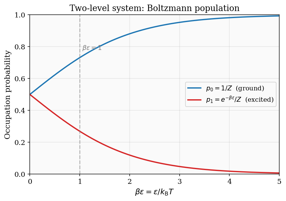
Figure 1: Occupation probabilities of a two-level system as a function of \(\beta\varepsilon = \varepsilon/k_{\rm B}T\). At low temperature the ground state dominates; at high temperature both levels approach equal occupation.

The partition function as a generating function

The partition function \(Z(\beta)\) is far more than a normalisation constant. All equilibrium properties of the system can be derived from it by differentiation.

Average energy. Since \(\langle E\rangle = \sum_s E_s P(s) = \sum_s E_s e^{-\beta E_s}/Z\), we recognise that \(\partial Z / \partial(-\beta) = \sum_s E_s e^{-\beta E_s}\). Therefore

\[ \langle E \rangle = -\frac{\partial \ln Z}{\partial \beta}. \]

Entropy and Helmholtz free energy. From the thermodynamic identity \(F = -k_{\rm B}T\ln Z\), all other potentials follow by standard Legendre transforms. The entropy is \(S = -\partial F/\partial T\), the pressure is \(p = -\partial F/\partial V\), and the heat capacity at constant volume is

\[ C_V = \frac{\partial \langle E \rangle}{\partial T} = k_{\rm B}\beta^2\frac{\partial^2 \ln Z}{\partial\beta^2}. \]

Energy fluctuations and the variance

The heat capacity can be related to the fluctuations in energy in a compelling way. Consider

\[ \langle E^2\rangle = \frac{1}{Z}\sum_s E_s^2\, e^{-\beta E_s} = \frac{1}{Z}\frac{\partial^2 Z}{\partial\beta^2}. \]

The variance in energy is \(\langle(\Delta E)^2\rangle = \langle E^2\rangle - \langle E\rangle^2\). After some algebra using the expressions above:

\[ \langle(\Delta E)^2\rangle = \frac{\partial^2\ln Z}{\partial\beta^2} = -\frac{\partial\langle E\rangle}{\partial\beta} = k_{\rm B}T^2\frac{\partial\langle E\rangle}{\partial T} = k_{\rm B}T^2 C_V. \]

This is a profound result. The fluctuations in energy of a system in contact with a heat bath are directly proportional to its heat capacity. A large heat capacity means the system can absorb energy without changing temperature, which in turn means many different microstates have similar energies — precisely the condition for large fluctuations. The relative fluctuation is

\[ \frac{\sqrt{\langle(\Delta E)^2\rangle}}{\langle E\rangle} = \frac{\sqrt{k_{\rm B}T^2 C_V}}{\langle E\rangle}. \]

For a monatomic ideal gas, \(C_V = \tfrac{3}{2}Nk_{\rm B}\) and \(\langle E\rangle = \tfrac{3}{2}Nk_{\rm B}T\), so the relative fluctuation is \(1/\sqrt{N} \sim 10^{-12}\). Thermal fluctuations are utterly negligible for macroscopic systems — another reason statistical mechanics predictions are effectively exact.

A worked example: the harmonic oscillator

The quantum harmonic oscillator with energy levels \(E_n = n\hbar\omega\) (measuring from the ground state, dropping the zero-point energy \(\hbar\omega/2\) for convenience) provides a clean illustration of the partition function machinery. The partition function is a geometric series:

\[ Z = \sum_{n=0}^\infty e^{-\beta n\hbar\omega} = \frac{1}{1 - e^{-\beta\hbar\omega}}. \]

The average energy follows from differentiation:

\[ \langle E\rangle = -\frac{\partial\ln Z}{\partial\beta} = \frac{\hbar\omega}{e^{\beta\hbar\omega} - 1}. \]

This is the Planck function for a single mode, familiar from blackbody radiation. The heat capacity of a single oscillator is

\[ C = \frac{\partial\langle E\rangle}{\partial T} = k_{\rm B}\left(\frac{\hbar\omega}{k_{\rm B}T}\right)^2 \frac{e^{\hbar\omega/k_{\rm B}T}}{(e^{\hbar\omega/k_{\rm B}T}-1)^2}. \]

Two limits are worth examining explicitly. At high temperature (\(k_{\rm B}T \gg \hbar\omega\), i.e.\ \(\beta\hbar\omega \ll 1\)): the exponential expands as \(e^{\beta\hbar\omega} \approx 1 + \beta\hbar\omega\), so \(\langle E\rangle \approx k_{\rm B}T\) and \(C \approx k_{\rm B}\). This is the classical equipartition result — one unit of \(k_{\rm B}T\) per quadratic degree of freedom (here the average of kinetic and potential energy each giving \(\tfrac{1}{2}k_{\rm B}T\)). At low temperature (\(k_{\rm B}T \ll \hbar\omega\)), the denominator \(e^{\beta\hbar\omega} - 1 \approx e^{\beta\hbar\omega}\) is exponentially large, so \(\langle E\rangle \approx \hbar\omega\, e^{-\hbar\omega/k_{\rm B}T} \to 0\) and \(C \approx k_{\rm B}(\hbar\omega/k_{\rm B}T)^2 e^{-\hbar\omega/k_{\rm B}T} \to 0\) exponentially. The oscillator is frozen out — it is almost certainly in its ground state, and the small probability of excitation to the first level decreases exponentially with decreasing temperature. This exponential quenching is the signature of an energy gap: modes with \(\hbar\omega \gg k_{\rm B}T\) are quantum-mechanically frozen and do not contribute to the heat capacity.

The ensemble in which \(T\) is fixed and \(N\) and \(V\) are fixed is the canonical ensemble. The probability distribution \(P(s) \propto e^{-\beta E_s}\) is the Boltzmann distribution, and \(Z\) is its partition function.

Equivalence of ensembles and thermodynamic limits

A subtlety that deserves mention: the microcanonical, canonical, and grand canonical ensembles are, in principle, different probability distributions over microstates — the first fixes \(E\), the second fixes \(T\), the third fixes both \(T\) and \(\mu\). For a finite system they give different predictions for thermodynamic quantities. However, in the thermodynamic limit (\(N\to\infty\), \(V\to\infty\) with \(N/V = \text{const}\)), all three ensembles give identical predictions for intensive quantities like pressure, temperature, and density. This is the equivalence of ensembles, which holds whenever thermodynamic fluctuations are negligible — i.e.\ whenever \(N\) is large. We have already seen this: the relative energy fluctuation in the canonical ensemble is \(\sim 1/\sqrt{N}\), which vanishes as \(N\to\infty\), so the canonical distribution is effectively a delta function around the average energy in the thermodynamic limit, equivalent to the microcanonical distribution at that energy.

Ensemble inequivalence does occur in systems with long-range interactions (gravitational systems, plasmas, certain spin models) where energy is not extensive. In such systems, the canonical ensemble may predict phase transitions that the microcanonical ensemble does not, or vice versa. But for the systems we consider in this course — short-range interactions, extensive energy — ensemble equivalence is a reliable theorem that frees us to choose whatever ensemble is most convenient for calculation.

---

Chapter 3: Working with the Partition Function

Degeneracy and thermal excitation

When multiple microstates share the same energy, we say those states are degenerate. For a state with energy \(E_n\) and degeneracy \(g_n\), the partition function takes the form \(Z = \sum_n g_n e^{-\beta E_n}\), and the probability of finding the system with energy \(E_n\) is \(P_n = g_n e^{-\beta E_n}/Z\).

As a concrete example, consider a hydrogen atom in thermal equilibrium at temperature \(T\). The energy levels are \(E_n = -13.6\ \text{eV}/n^2\) with degeneracy \(g_n = 2n^2\) (counting spin and orbital angular momentum). At room temperature \(k_{\rm B}T \approx 0.025\ \text{eV}\), which is much smaller than the excitation energy of the first excited state, \(E_2 - E_1 \approx 10.2\ \text{eV}\). The Boltzmann factor \(e^{-\beta(E_2-E_1)} \approx e^{-408}\) is so tiny that essentially all hydrogen atoms are in the ground state. Only near the surface of a star, where \(T \sim 10^4\ \text{K}\) and \(k_{\rm B}T \sim 1\ \text{eV}\), does the first excited state begin to be significantly populated. This explains the strength of the Balmer absorption lines in stellar spectra: the \(n=2\) level has just enough thermal population to absorb visible photons.

The paramagnet revisited

The two-state paramagnet is the workhorse example of Chapter 2, and it pays to extract every physical quantity from its partition function. A spin-\(\tfrac{1}{2}\) dipole in field \(B\) (along \(\hat{z}\)) has energies \(E_\uparrow = -\mu B\) and \(E_\downarrow = +\mu B\), so

\[ Z = e^{\beta\mu B} + e^{-\beta\mu B} = 2\cosh(\beta\mu B). \]

The average energy of a single dipole is

\[ \langle E \rangle = -\mu B\tanh(\beta\mu B), \]

and the average component of the dipole along \(\hat{z}\) is \(\langle\mu_z\rangle = \mu\tanh(\beta\mu B)\). For \(N\) independent dipoles the total magnetisation is

\[ M = N\mu\tanh(\beta\mu B). \]

Two limits illuminate the physics. At high temperature (\(k_{\rm B}T \gg \mu B\), i.e.\ \(\beta\mu B \to 0\)), \(\tanh x \approx x\) and \(M \approx N\mu^2 B / (k_{\rm B}T)\): the magnetisation is inversely proportional to temperature. This is Curie’s law, \(M \propto 1/T\), which can be understood qualitatively by noting that thermal fluctuations compete with the field in aligning the spins. At low temperature (\(\beta\mu B \to \infty\)), \(\tanh \to 1\) and \(M \to N\mu\): all spins align with the field. The transition between these regimes occurs on the scale \(k_{\rm B}T \sim \mu B\).

Heat capacity and the Schottky anomaly

To find the heat capacity of the paramagnet, differentiate the total energy \(U = -N\mu B\tanh(\beta\mu B)\) with respect to \(T\). Using \(\partial\tanh(\beta\mu B)/\partial T = -(\mu B/k_{\rm B}T^2)\operatorname{sech}^2(\beta\mu B)\):

\[ C = \frac{\partial U}{\partial T} = Nk_{\rm B}(\beta\mu B)^2\operatorname{sech}^2(\beta\mu B). \]

This heat capacity has a striking feature: it is not monotonic. As \(T\to 0\), \(\beta\mu B\to\infty\) and \(\operatorname{sech}^2(\beta\mu B)\to 0\) exponentially, so \(C\to 0\). As \(T\to\infty\), \(\beta\mu B\to 0\) and \((\beta\mu B)^2\operatorname{sech}^2(\beta\mu B)\to 0\) as \(\beta^2\to 0\), so \(C\to 0\) again. In between, \(C\) passes through a maximum — the Schottky anomaly — at a temperature \(k_{\rm B}T_{\rm peak}\approx 0.83\,\mu B\), where the thermal energy is comparable to the level splitting. The physical picture is clear: at low \(T\) the system is frozen in the ground state and cannot absorb heat; at high \(T\) the two levels are equally populated and further heating changes nothing; at intermediate \(T\) the system is actively transitioning between the two levels and absorbs heat efficiently. Any two-level system (atomic hyperfine levels, crystal-field split electronic levels, nuclear spin states) exhibits this anomalous peak in \(C(T)\), providing a direct spectroscopic tool for measuring energy splittings.

Negative temperature in two-level systems

Because the energy of a two-level spin system is bounded above (you cannot put more than \(N\mu B\) of energy into a paramagnet), it is possible to prepare states that are genuinely hotter than any state with positive temperature. If the population of the upper energy level exceeds that of the lower level, the system is in a population inversion. Adding more energy to such a state increases the disorder (the system was already highly ordered by the inversion, and more energy makes the populations more equal), so \(\partial S/\partial E > 0\) initially but eventually \(\partial S/\partial E < 0\) once the populations cross equal occupation.

More precisely: the entropy of a two-level system with \(N_\uparrow\) spins up and \(N_\downarrow = N - N_\uparrow\) spins down is \(S = k_{\rm B}\ln\binom{N}{N_\uparrow}\). The energy is \(U = -(N_\uparrow - N_\downarrow)\mu B = -(2N_\uparrow - N)\mu B\). As \(N_\uparrow\) increases from \(0\) to \(N/2\), \(S\) increases (more disorder) and so does \(U\) — giving \(\partial S/\partial U > 0\) and positive temperature. As \(N_\uparrow\) increases from \(N/2\) to \(N\), \(S\) decreases (the system becomes more ordered again, now with most spins up) while \(U\) continues to increase — giving \(\partial S/\partial U < 0\) and thus \(T < 0\). The Boltzmann distribution still holds: a population inversion corresponds to a \(\beta < 0\) Boltzmann weight \(e^{-\beta E_s}\) that favours higher energies. A system at negative temperature is hotter than any positive-temperature system in the sense that energy flows from it to any positive-temperature body on thermal contact. The temperature sequence, ordered from cold to hot, is \(T = 0^+, \ldots, +\infty \equiv -\infty, \ldots, T = 0^-\).

A practically important technique for the low-temperature regime: write \(\tanh(\beta\mu B) = (1 - e^{-2\beta\mu B})/(1+e^{-2\beta\mu B}) \approx 1 - 2e^{-2\beta\mu B}\) for large \(\beta\mu B\). The leading correction to full saturation is exponentially small, a signature of the energy gap \(2\mu B\) separating the ground state from the first excited state.

The rotational partition function

Diatomic molecules — nitrogen, oxygen, hydrogen — have rotational degrees of freedom that become thermally accessible at temperatures well below room temperature for light molecules. A rigid rotor has energy levels

\[ E_J = \varepsilon_{\rm rot}\, J(J+1), \qquad J = 0, 1, 2, \ldots, \]

with degeneracy \(2J+1\), where \(\varepsilon_{\rm rot} = \hbar^2/(2I)\) and \(I\) is the moment of inertia. The partition function is

\[ Z_{\rm rot} = \sum_{J=0}^\infty (2J+1)\,e^{-\beta\varepsilon_{\rm rot}J(J+1)}. \]

This sum does not have a closed form. However, in the high-temperature limit (\(\beta\varepsilon_{\rm rot} \ll 1\)) the levels are densely packed relative to \(k_{\rm B}T\), and the sum can be replaced by an integral. With the substitution \(u = J(J+1)\), \(du = (2J+1)\,dJ\):

\[ Z_{\rm rot} \approx \int_0^\infty (2J+1)\,e^{-\beta\varepsilon_{\rm rot}J(J+1)}\,dJ = \frac{1}{\beta\varepsilon_{\rm rot}} = \frac{k_{\rm B}T}{\varepsilon_{\rm rot}}. \]

The average rotational energy follows immediately:

\[ \langle E_{\rm rot}\rangle = -\frac{\partial\ln Z_{\rm rot}}{\partial\beta} = k_{\rm B}T. \]

This is a preview of the equipartition theorem: each quadratic degree of freedom (here the two rotational angles of a diatomic molecule) contributes \(\tfrac{1}{2}k_{\rm B}T\) to the average energy.

The low-temperature limit. At low temperature (\(\beta\varepsilon_{\rm rot} \gg 1\)), only the lowest few terms in \(Z_{\rm rot}\) matter. Retaining \(J = 0\) and \(J = 1\):

\[ Z_{\rm rot} \approx 1 + 3e^{-2\beta\varepsilon_{\rm rot}}, \]

since the \(J=1\) level has degeneracy \(2(1)+1 = 3\) and energy \(\varepsilon_{\rm rot}\cdot 1\cdot 2 = 2\varepsilon_{\rm rot}\). The average energy is approximately \(\langle E_{\rm rot}\rangle \approx 6\varepsilon_{\rm rot}e^{-2\beta\varepsilon_{\rm rot}}/(1 + 3e^{-2\beta\varepsilon_{\rm rot}})\), which is exponentially suppressed. The rotational heat capacity is similarly suppressed, approaching zero exponentially as \(T\to 0\). The crossover temperature is set by \(\varepsilon_{\rm rot}/k_{\rm B}\), which takes different values for different molecules:

Molecule	\(\varepsilon_{\rm rot}/k_{\rm B}\) (K)
H\(_2\)	85.4
N\(_2\)	2.88
O\(_2\)	2.08

For nitrogen and oxygen, \(\varepsilon_{\rm rot}/k_{\rm B}\) is only a few kelvin, well below room temperature, so rotation is fully excited at ambient conditions and contributes \(k_{\rm B}T\) to the energy and \(k_{\rm B}\) to the heat capacity per molecule. For hydrogen, \(\varepsilon_{\rm rot}/k_{\rm B} = 85.4\ \text{K}\) means that at room temperature \(\beta\varepsilon_{\rm rot} \approx 0.29\) and the high-temperature approximation is marginal — this is why the rotational heat capacity of H\(_2\) is not fully activated at room temperature.

A subtle complication arises for homonuclear diatomics (H\(_2\), N\(_2\), O\(_2\)), where the two identical nuclei impose exchange-symmetry constraints on the wave function. For hydrogen in particular, the nuclear spin state (ortho or para hydrogen) selects either even or odd values of \(J\), effectively halving the number of accessible states at low temperature.

The Einstein solid from the partition function

For a collection of \(N\) independent quantum harmonic oscillators, each at frequency \(\omega\), the partition function factorises as \(Z_N = Z_1^N\) (distinguishable oscillators on a lattice). The average energy is simply \(N\) times the single-oscillator result derived above:

\[ \langle E\rangle = \frac{N\hbar\omega}{e^{\beta\hbar\omega}-1}, \]

and the heat capacity is

\[ C_V = Nk_{\rm B}\left(\frac{\hbar\omega}{k_{\rm B}T}\right)^2\frac{e^{\hbar\omega/k_{\rm B}T}}{(e^{\hbar\omega/k_{\rm B}T}-1)^2}. \]

At high temperature this approaches \(Nk_{\rm B}\) per degree of freedom — for a 3D solid with \(3N\) modes, \(C_V\to 3Nk_{\rm B}\), which is the Dulong–Petit law, confirmed experimentally for many materials at sufficiently high temperature. At low temperature the heat capacity is exponentially suppressed: \(C_V \propto (\hbar\omega/k_{\rm B}T)^2 e^{-\hbar\omega/k_{\rm B}T}\to 0\). The Einstein model’s prediction of exponential low-\(T\) quenching is qualitatively correct (it captures the freezing-out of quantum modes) but quantitatively wrong (real solids show a power-law \(T^3\) rather than exponential decay), because a real solid has a spectrum of vibrational frequencies, not a single frequency. The Debye model, treated in Chapter 11, fixes this.

Composite systems and factorisation

If a system decomposes into independent subsystems A and B, with energies \(E_A\) and \(E_B\), the total energy is \(E = E_A + E_B\) and the microstates factorise. The partition function factorises too:

\[ Z = \sum_{s_A, s_B} e^{-\beta(E_{s_A} + E_{s_B})} = Z_A \cdot Z_B. \]

Taking logarithms: \(\ln Z = \ln Z_A + \ln Z_B\), so the free energy \(F = -k_{\rm B}T\ln Z\) is additive. This is why extensive thermodynamic quantities (energy, entropy, free energy) are additive for non-interacting subsystems.

The factorisation property has a profound implication for the partition function of a complex molecule. Any system whose Hamiltonian can be written as a sum of independent terms \(H = H_1 + H_2 + \ldots\) has a partition function that factorises as \(Z = Z_1 Z_2\cdots\). This means we can compute the thermal properties of each part separately and combine them by addition of free energies. For a diatomic gas, the translational, rotational, vibrational, and electronic degrees of freedom all satisfy this condition (to a good approximation), and their separate partition functions, computed in Chapters 2 and 3, immediately give the full thermodynamics of the molecule. The factorisation is the partition function’s reflection of the extensivity of thermodynamics.

---

Chapter 4: Continuous Degrees of Freedom and the Maxwell–Boltzmann Distribution

Phase space and classical partition functions

Discrete energy levels are the quantum-mechanical default, but at sufficiently high temperatures the level spacings become negligible compared to \(k_{\rm B}T\) and we can treat position and momentum as continuous variables. The classical partition function for a single particle moving in three dimensions is

\[ Z_1 = \frac{1}{h^3}\int d^3x\,d^3p\; e^{-\beta p^2/(2m)} = \frac{V}{\lambda_{\rm dB}^3}, \]

where \(\lambda_{\rm dB} = h/\sqrt{2\pi m k_{\rm B}T}\) is the thermal de Broglie wavelength. The factor of \(h^3\) in the denominator is Planck’s constant cubed — it sets the minimum volume of a cell in phase space, preventing the integral from diverging and maintaining the correct classical limit of the quantum result. The thermal de Broglie wavelength sets the length scale below which quantum effects become important: when the typical inter-particle separation \((V/N)^{1/3}\) is much larger than \(\lambda_{\rm dB}\), the gas behaves classically.

The three-dimensional momentum integral

Let us evaluate the momentum integral explicitly, since this Gaussian integral reappears throughout the course. Write the three-dimensional integral as a product over Cartesian components:

\[ \int d^3p\; e^{-\beta p^2/(2m)} = \left(\int_{-\infty}^{\infty} e^{-\beta p_x^2/(2m)}\,dp_x\right)^3. \]

Each one-dimensional Gaussian integral evaluates to \(\sqrt{2\pi m/\beta} = \sqrt{2\pi mk_{\rm B}T}\) using the standard result \(\int_{-\infty}^\infty e^{-ax^2}\,dx = \sqrt{\pi/a}\). Therefore

\[ \int d^3p\; e^{-\beta p^2/(2m)} = (2\pi mk_{\rm B}T)^{3/2}. \]

Combining with the spatial integral \(\int d^3x = V\) and the phase-space prefactor \(1/h^3\):

\[ Z_1 = \frac{V(2\pi mk_{\rm B}T)^{3/2}}{h^3} = \frac{V}{\lambda_{\rm dB}^3}, \qquad \lambda_{\rm dB} = \frac{h}{\sqrt{2\pi mk_{\rm B}T}}. \]

This is the fundamental result for the single-particle translational partition function of a classical particle.

The equipartition theorem

For any quadratic degree of freedom — any term of the form \(\tfrac{1}{2}a x^2\) in the Hamiltonian, whether \(x\) is a momentum component or a displacement — the contribution to the average energy is exactly \(\tfrac{1}{2}k_{\rm B}T\). Formally, this follows from the Gaussian integral: the Boltzmann weight \(e^{-\beta a x^2/2}\) gives \(\langle\tfrac{1}{2}ax^2\rangle = \tfrac{1}{2}k_{\rm B}T\). Counting degrees of freedom then immediately predicts heat capacities:

System	Degrees of freedom	\(C_V / Nk_{\rm B}\)
Monatomic ideal gas	3 translational	\(\tfrac{3}{2}\)
Diatomic (high \(T\))	3 trans + 2 rot	\(\tfrac{5}{2}\)
Diatomic (very high \(T\))	3 trans + 2 rot + 2 vib	\(\tfrac{7}{2}\)
3D harmonic solid	3 kin + 3 pot	3 (Dulong-Petit)

The activation of rotational and vibrational modes at increasing temperatures is visible in the measured heat capacity of hydrogen gas, rising from \(\tfrac{3}{2}\) at cryogenic temperatures through \(\tfrac{5}{2}\) at room temperature toward \(\tfrac{7}{2}\) above \(\sim 3000\ \text{K}\).

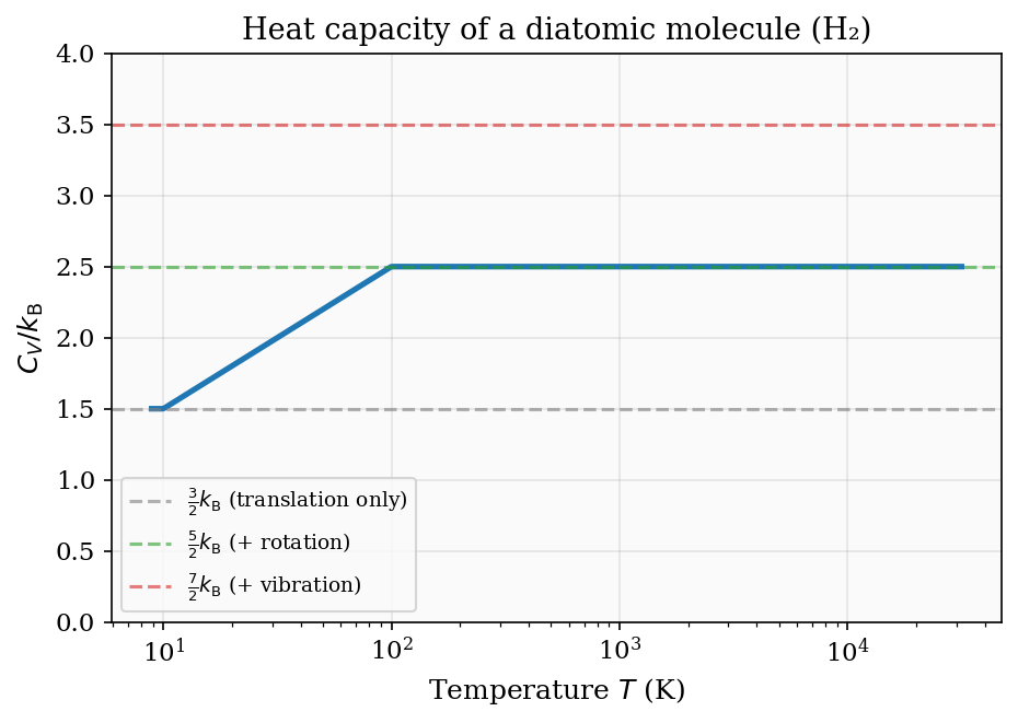
Figure 4: Schematic heat capacity of a diatomic molecule. The plateaus at \(\tfrac{3}{2}\), \(\tfrac{5}{2}\), and \(\tfrac{7}{2}\) correspond to translational, rotational, and vibrational degrees of freedom becoming active as temperature rises.

The Maxwell–Boltzmann speed distribution

The Boltzmann factor applied to a gas molecule with velocity \(\mathbf{v}\) gives a probability density proportional to \(e^{-mv^2/2k_{\rm B}T}\) in velocity space. Converting to a distribution over speed \(v = |\mathbf{v}|\) by integrating over the spherical shell of radius \(v\) in 3D velocity space:

\[ f(v) = 4\pi \left(\frac{m}{2\pi k_{\rm B}T}\right)^{3/2} v^2\, e^{-mv^2/2k_{\rm B}T}. \]

The factor \(v^2\) (surface area of the sphere) and the exponential (Boltzmann weight) together create a distribution with a well-defined most-probable speed \(v_p = \sqrt{2k_{\rm B}T/m}\), a mean speed \(\langle v\rangle = \sqrt{8k_{\rm B}T/\pi m}\), and an rms speed \(\sqrt{\langle v^2\rangle} = \sqrt{3k_{\rm B}T/m}\).

Deriving the mean and rms speeds from Gaussian integrals. The relevant integrals are of the form \(\int_0^\infty v^n e^{-v^2/v_0^2}\,dv\), where \(v_0 = \sqrt{2k_{\rm B}T/m}\). For the normalisation, \(n=2\): \(\int_0^\infty v^2 e^{-v^2/v_0^2}\,dv = \sqrt{\pi}v_0^3/4\). The mean speed uses \(n=3\): \(\int_0^\infty v^3 e^{-v^2/v_0^2}\,dv = v_0^4/2\). The mean-square speed uses \(n=4\): \(\int_0^\infty v^4 e^{-v^2/v_0^2}\,dv = 3\sqrt{\pi}v_0^5/8\). Combining these with the normalisation factor \(4\pi(m/2\pi k_{\rm B}T)^{3/2} = 4/(\sqrt{\pi}v_0^3)\):

\[ \langle v\rangle = \frac{4}{\sqrt{\pi}v_0^3}\cdot\frac{v_0^4}{2} = \frac{2v_0}{\sqrt{\pi}} = \sqrt{\frac{8k_{\rm B}T}{\pi m}}, \]\[ \langle v^2\rangle = \frac{4}{\sqrt{\pi}v_0^3}\cdot\frac{3\sqrt{\pi}v_0^5}{8} = \frac{3v_0^2}{2} = \frac{3k_{\rm B}T}{m}, \]

so the rms speed is \(v_{\rm rms} = \sqrt{3k_{\rm B}T/m}\). All three characteristic speeds grow as \(\sqrt{T}\) and decrease as \(1/\sqrt{m}\) — heavier molecules move slower at the same temperature, which underlies the phenomenon of effusion.

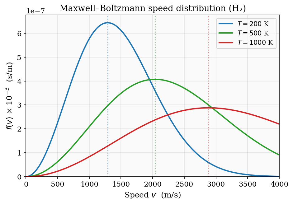
Figure 3: The Maxwell–Boltzmann speed distribution for H\(_2\) at 200 K, 500 K, and 1000 K. The peak shifts to higher speeds and the distribution broadens as temperature increases; dotted vertical lines mark the most-probable speed \(v_p\).

Effusion and Graham’s law

Effusion is the process by which gas molecules escape through a small hole in a container wall — small enough that the equilibrium Maxwell–Boltzmann distribution is not disturbed. The flux of molecules hitting a unit area of wall per unit time is

\[ \Phi = \int_{v_z > 0} v_z\, f(v)\,d^3v, \]

where the integral is over all velocities with positive \(z\)-component (moving toward the wall). Writing \(f(v)\,d^3v = f(v_x, v_y, v_z)\,dv_x\,dv_y\,dv_z\) and using the fact that \(v_z\) and \(v_x, v_y\) are independent:

\[ \Phi = n\int_0^\infty v_z\left(\frac{m}{2\pi k_{\rm B}T}\right)^{1/2}e^{-mv_z^2/2k_{\rm B}T}\,dv_z = n\sqrt{\frac{k_{\rm B}T}{2\pi m}} = \frac{n\langle v\rangle}{4}, \]

where \(n = N/V\) is the number density. The result \(\Phi = n\langle v\rangle/4\) is the standard effusion formula. Since \(\langle v\rangle \propto 1/\sqrt{m}\), the effusion rate is inversely proportional to the square root of the molecular mass — this is Graham’s law of effusion. Lighter gases escape through a pinhole faster; historically this was used to separate uranium isotopes (\(^{235}\)UF\(_6\) vs \(^{238}\)UF\(_6\)) by repeated effusion through porous barriers.

The barometric formula

The Boltzmann factor applies to any form of energy, not just kinetic energy. A molecule at height \(z\) in Earth’s atmosphere has gravitational potential energy \(U = mgz\). The probability of finding a molecule at height \(z\) is therefore proportional to \(e^{-mgz/k_{\rm B}T}\), and since the number density \(n(z)\) is proportional to this probability:

\[ n(z) = n_0\, e^{-mgz/k_{\rm B}T} = n_0\, e^{-z/H}, \]

where the scale height is \(H = k_{\rm B}T/(mg)\). This is the barometric formula, also called the law of atmospheres. For nitrogen (the dominant constituent of Earth’s atmosphere, with \(m \approx 4.65\times 10^{-26}\ \text{kg}\)) at \(T = 250\ \text{K}\):

\[ H = \frac{k_{\rm B}T}{mg} = \frac{(1.38\times 10^{-23})(250)}{(4.65\times 10^{-26})(9.8)} \approx 7.6\ \text{km}. \]

The atmospheric pressure falls to \(1/e \approx 37\%\) of its sea-level value at \(z \approx 7.6\ \text{km}\), consistent with the observation that Mount Everest (8.8 km) has roughly one-third of sea-level atmospheric pressure. The exponential dependence on \(mgz/k_{\rm B}T\) is a direct consequence of the Boltzmann factor — the atmosphere is a system in thermal equilibrium (approximately) with a spatially varying external potential.

It is worth noting that the barometric formula is consistent with hydrostatic equilibrium. The pressure gradient required to support the weight of the gas is \(dp/dz = -\rho g = -nmg\). The ideal gas law \(p = nk_{\rm B}T\) (at constant \(T\)) gives \(dp = k_{\rm B}T\,dn\), so \(k_{\rm B}T\,dn/dz = -nmg\), or \(dn/n = -mg\,dz/(k_{\rm B}T)\). Integrating recovers the barometric formula. The Boltzmann statistical argument and the fluid mechanical hydrostatic argument are two perspectives on the same result, connected by the thermodynamic equation of state.

Isothermal versus adiabatic atmospheres. The barometric formula assumes a constant temperature \(T\), which is an approximation. In reality, the temperature of the atmosphere decreases with altitude at a rate of about \(6.5\ \text{K/km}\) in the troposphere (the adiabatic lapse rate, set by the condition that a rising air parcel expands adiabatically without becoming buoyantly unstable). At higher altitudes (stratosphere and above), the temperature profile is more complex. The barometric formula with a constant \(T\) is a good approximation for order-of-magnitude estimates and for understanding the basic physics; a more accurate treatment requires solving the coupled equations of hydrostatics, thermodynamics, and radiative transfer.

The derivation also illustrates a general principle: in the local density approximation (LDA), a system in an external potential \(U(\mathbf{r})\) has a local chemical potential \(\mu_{\rm local}(\mathbf{r}) = \mu - U(\mathbf{r})\), and the local density is whatever density gives the right \(\mu_{\rm local}\). This generalisation will be important when we study trapped atomic gases in Chapter 14.

---

Chapter 5: The Grand Canonical Ensemble

Chemical potential and particle exchange

The canonical ensemble holds \(N\) fixed. Many physical situations involve particle exchange: a metal in contact with an electron reservoir, a gas in contact with a larger gas, a protein that can bind or release ligand molecules. The relevant ensemble allows both energy and particle number to fluctuate.

The chemical potential \(\mu\) is the thermodynamic variable conjugate to particle number, defined by

\[ \mu = \left(\frac{\partial U}{\partial N}\right)_{S,V} = \left(\frac{\partial F}{\partial N}\right)_{T,V}. \]

Just as temperature drives energy to flow from high-\(T\) to low-\(T\) regions until equilibrium is reached, chemical potential drives particles to flow from high-\(\mu\) to low-\(\mu\) regions until the chemical potentials equalise. This is diffusive equilibrium.

Diffusive equilibrium from entropy maximisation

The condition for diffusive equilibrium follows from the same entropy-maximisation argument we used for thermal equilibrium. Consider two systems with particle numbers \(N_1\) and \(N_2\), with \(N_1 + N_2 = N_{\rm tot}\) fixed, in contact at the same temperature \(T\). The total entropy is \(S_{\rm tot}(N_1) = S_1(N_1) + S_2(N_{\rm tot} - N_1)\). Maximising over \(N_1\):

\[ \frac{\partial S_{\rm tot}}{\partial N_1} = \frac{\partial S_1}{\partial N_1} - \frac{\partial S_2}{\partial N_2} = 0 \quad \Rightarrow \quad \frac{\partial S_1}{\partial N_1}\bigg|_{E,V} = \frac{\partial S_2}{\partial N_2}\bigg|_{E,V}. \]

The thermodynamic identity \(dU = T\,dS - p\,dV + \mu\,dN\) gives \(\partial S/\partial N|_{E,V} = -\mu/T\), so the equilibrium condition is \(-\mu_1/T = -\mu_2/T\), i.e.\ \(\mu_1 = \mu_2\). Particles flow from high \(\mu\) to low \(\mu\), exactly as heat flows from high \(T\) to low \(T\).

By extending the Boltzmann argument — now treating a system in contact with a reservoir of both energy and particles — one finds that the probability of a microstate \(s\) with energy \(E_s\) and particle number \(N_s\) is

\[ P(s) = \frac{1}{\mathcal{Z}}\,e^{-\beta(E_s - \mu N_s)}, \]

where the grand partition function (also called the grand sum) is

\[ \mathcal{Z} = \sum_{s} e^{-\beta(E_s - \mu N_s)} = \sum_{N=0}^\infty e^{\beta\mu N}\,Z_N, \]

with \(Z_N\) the \(N\)-particle canonical partition function. The average particle number is \(\langle N\rangle = k_{\rm B}T\,\partial\ln\mathcal{Z}/\partial\mu\), and the average energy is \(\langle E\rangle = -\partial\ln\mathcal{Z}/\partial\beta + \mu\langle N\rangle\).

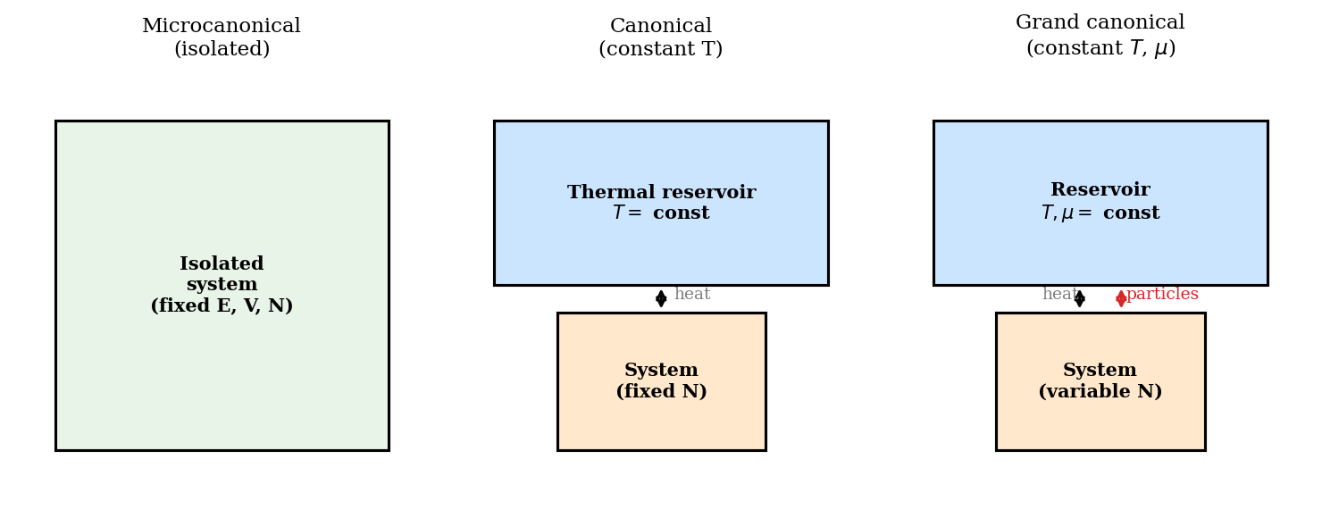
Figure 2: The three ensembles. In the microcanonical (left) the system is isolated; in the canonical (centre) it can exchange heat with a reservoir at temperature \(T\); in the grand canonical (right) it exchanges both heat and particles with a reservoir at temperature \(T\) and chemical potential \(\mu\).

The grand potential

The thermodynamic potential naturally associated with the grand canonical ensemble is the grand potential:

\[ \Phi = -k_{\rm B}T\ln\mathcal{Z} = U - TS - \mu\langle N\rangle. \]

All thermodynamic quantities follow from derivatives of \(\Phi\). The entropy is

\[ S = -\frac{\partial\Phi}{\partial T}\bigg|_{\mu,V}, \]

the mean particle number is

\[ \langle N\rangle = -\frac{\partial\Phi}{\partial\mu}\bigg|_{T,V}, \]

and the pressure is

\[ p = -\frac{\partial\Phi}{\partial V}\bigg|_{T,\mu}. \]

For an ideal gas, \(\Phi = -k_{\rm B}T\mathcal{Z}\), and these derivatives reproduce the ideal gas law and the Sackur–Tetrode entropy. The grand potential plays the same role for the grand canonical ensemble that the Helmholtz free energy \(F\) plays for the canonical ensemble: it is the appropriate free energy to minimise when \(T\) and \(\mu\) (rather than \(T\) and \(N\)) are the natural variables.

A biological application: haemoglobin

The grand canonical ensemble provides a beautiful model of how haemoglobin carries oxygen in the blood. Treat each of the four binding sites on a haemoglobin molecule as an independent two-state system: either empty (energy \(0\), one particle) or occupied by an O\(_2\) molecule (energy \(-\varepsilon < 0\), counts as one additional particle). The grand partition function for a single site is

\[ \mathcal{Z}_{\rm site} = 1 + e^{\beta(\mu + \varepsilon)}, \]

and the average occupation (fraction of the time the site is occupied by oxygen) is

\[ \langle n\rangle = \frac{e^{\beta(\mu+\varepsilon)}}{1 + e^{\beta(\mu+\varepsilon)}} = \frac{1}{1 + e^{-\beta(\mu+\varepsilon)}}. \]

This is a Fermi–Dirac-like distribution, even though we are dealing with a classical binding problem; the underlying reason is that the site is either empty or singly occupied (occupation restricted to 0 or 1), which is the same restriction that gives fermions their statistics.

In the blood, \(\mu\) is determined by the partial pressure of oxygen: higher O\(_2\) pressure \(\Rightarrow\) larger \(\mu\) (by the ideal gas relation \(\mu = k_{\rm B}T\ln(P/P_0)\)). In the lungs, O\(_2\) pressure is high, \(\mu\) is large, and \(\langle n\rangle\) is close to 1 — the haemoglobin loads up with oxygen. In peripheral tissues where O\(_2\) is consumed, the pressure is lower, \(\mu\) drops, and \(\langle n\rangle\) decreases — oxygen is released. The operating point in the lungs corresponds roughly to \(\langle n\rangle \approx 0.95\) while in resting tissue the operating point is \(\langle n\rangle \approx 0.7\), releasing about a quarter of the oxygen with each pass. Under exercise, the tissue O\(_2\) partial pressure drops further and \(\langle n\rangle\) falls to \(0.3\)–\(0.5\), releasing much more oxygen per cycle.

Real haemoglobin has cooperative binding among the four sites — binding one O\(_2\) makes it easier for the subsequent sites to bind, giving a sigmoidal loading curve that is steeper than the single-site prediction. The Hill equation \(\langle n\rangle = p^h/(K^h + p^h)\) with Hill coefficient \(h \approx 2.8\) for haemoglobin captures this cooperativity phenomenologically; the single-site grand canonical result is recovered for \(h = 1\). The cooperative binding sharpens the loading/unloading switch, making haemoglobin a much more efficient oxygen transporter than a non-cooperative binder would be.

---

Chapter 6: The Classical Ideal Gas Re-derived

The quantum mechanical gas in a box

A structureless particle of mass \(m\) in a cubic box of side \(L\) has energy levels determined by the requirement that the wave function vanishes at the walls. For a particle in a box with standing-wave boundary conditions, the allowed wave vectors are \(k_i = n_i\pi/L\) with \(n_i = 1, 2, 3, \ldots\), giving energy levels

\[ E_{\mathbf{n}} = \frac{\hbar^2\pi^2}{2mL^2}\left(n_x^2 + n_y^2 + n_z^2\right) = \frac{h^2}{8mL^2}\left(n_x^2 + n_y^2 + n_z^2\right). \]

For a macroscopic box at room temperature, the ground-state energy \(h^2/8mL^2\) is of order \(10^{-38}\ \text{J}\) — many orders of magnitude below \(k_{\rm B}T \sim 10^{-21}\ \text{J}\). The levels are so densely packed that the single-particle partition function is well approximated by an integral over continuous \(\mathbf{n}\), or equivalently over continuous momentum. Switching to periodic boundary conditions (which give \(k_i = 2\pi n_i/L\) with \(n_i \in \mathbb{Z}\)) and converting the sum over lattice points in \(\mathbf{k}\)-space to an integral using the density of states \(V/(2\pi)^3\) per unit \(k^3\)-volume:

\[ Z_1 = \frac{V}{(2\pi)^3}\int d^3k\; e^{-\beta\hbar^2 k^2/(2m)} = \frac{V}{h^3}\int d^3p\; e^{-\beta p^2/(2m)} = V\left(\frac{2\pi m k_{\rm B}T}{h^2}\right)^{3/2} = \frac{V}{\lambda_{\rm dB}^3}. \]

This shows how the discrete quantum sum over states in a box becomes, in the classical limit, precisely the phase-space integral with the Planck cell volume \(h^3\). The quantum derivation thus justifies the classical phase-space prescription — there is no ambiguity about factors of \(h\).

Indistinguishability and the Gibbs paradox

For distinguishable particles the \(N\)-particle partition function would be \(Z_1^N\). But gas molecules are indistinguishable: swapping two identical molecules does not produce a new microstate. Naively using \(Z_N = Z_1^N\) for an ideal gas leads to a profound inconsistency known as the Gibbs paradox. Consider two portions of the same ideal gas: \(N/2\) molecules in volume \(V/2\) on the left, and \(N/2\) molecules in the same gas in volume \(V/2\) on the right. When the partition is removed, a classical calculation with \(Z_N = Z_1^N\) gives an entropy of mixing

\[ \Delta S_{\rm mixing} = Nk_{\rm B}\ln 2 > 0, \]

arising because each molecule now has twice the volume available. But physically, mixing two portions of the same gas should produce no entropy change — there is no way to tell whether a molecule in the combined system came from the left or right. The Gibbs paradox is an artificial entropy of mixing that arises from treating identical particles as distinguishable.

The resolution is to divide by \(N!\), accounting for the fact that permuting the \(N\) molecules does not produce a distinct microstate:

\[ Z_N = \frac{Z_1^N}{N!}. \]

With this correction, the entropy of mixing identical gases is exactly zero, as it must be. The division by \(N!\) is not a semiclassical patch — it is the correct classical limit of the quantum treatment of identical bosons or fermions when the phase-space density \(N\lambda_{\rm dB}^3/V \ll 1\). In the quantum treatment, identical bosons (fermions) have symmetric (antisymmetric) wave functions, and in the dilute limit the symmetrisation produces exactly the \(N!\) suppression of the partition function.

The Sackur-Tetrode entropy and the ideal gas law

From \(F = -k_{\rm B}T\ln Z_N\) we extract all ideal gas properties. Using Stirling’s approximation \(\ln N! \approx N\ln N - N\):

\[ F = Nk_{\rm B}T\left[\ln\!\left(\frac{N\lambda_{\rm dB}^3}{V}\right) - 1\right]. \]

The pressure is \(p = -\partial F/\partial V = Nk_{\rm B}T/V\), recovering the ideal gas law \(pV = Nk_{\rm B}T\) from a microscopic derivation. The entropy is

\[ S = Nk_{\rm B}\left[\ln\!\left(\frac{V}{N\lambda_{\rm dB}^3}\right) + \frac{5}{2}\right]. \]

This is the Sackur–Tetrode equation, derived independently by Sackur and Tetrode in 1911. It is remarkable for two reasons. First, it contains Planck’s constant \(h\) (through \(\lambda_{\rm dB}\)), so even the classical entropy of a gas knows about quantum mechanics. Second, it is extensive: if you double \(N\) and \(V\), the entropy doubles — the \(\ln(V/N)\) factor ensures this.

Numerical check for helium. At standard temperature and pressure (\(T = 273.15\ \text{K}\), \(p = 101.325\ \text{kPa}\)), the number density of helium (mass \(m = 4 \times 1.66\times 10^{-27}\ \text{kg}\)) is \(n = p/(k_{\rm B}T) \approx 2.69\times 10^{25}\ \text{m}^{-3}\). The thermal de Broglie wavelength is \(\lambda_{\rm dB} = h/\sqrt{2\pi mk_{\rm B}T} \approx 0.40\ \text{\AA}\). The Sackur–Tetrode formula gives

\[ \frac{S}{Nk_{\rm B}} = \ln\!\left(\frac{n^{-1}}{\lambda_{\rm dB}^3}\right) + \frac{5}{2} \approx \ln\!\left(\frac{(3.7\times 10^{-26})}{(6.4\times 10^{-32})}\right) + 2.5 \approx \ln(5.8\times 10^5) + 2.5 \approx 13.3 + 2.5 = 15.8. \]

The tabulated value for helium at STP is \(S/(Nk_{\rm B}) \approx 15.2\) — the Sackur–Tetrode prediction agrees to within a few percent. The small discrepancy comes from corrections beyond the ideal-gas approximation. The fact that this formula, derived purely from quantum mechanics and statistical mechanics, predicts the absolute entropy of a gas (not merely entropy differences) to such accuracy is a triumph.

The chemical potential of the ideal gas

The chemical potential follows from \(\mu = \partial F/\partial N\):

\[ \mu = k_{\rm B}T\ln\!\left(\frac{N\lambda_{\rm dB}^3}{V}\right). \]

This connects Chapters 5 and 6 directly. For a dilute classical gas, \(N\lambda_{\rm dB}^3/V \ll 1\) and \(\mu\) is large and negative — it costs no free energy to add a particle because the gas is sparse. As the gas is compressed (larger \(N/V\)) or cooled (larger \(\lambda_{\rm dB}\)), \(\mu\) rises toward zero. When \(\mu\) reaches zero, the phase-space density \(N\lambda_{\rm dB}^3/V \approx 1\) and quantum effects become dominant — this signals the onset of quantum degeneracy, the subject of Part II. For bosons, \(\mu = 0\) is the threshold for Bose–Einstein condensation; for fermions, \(\mu = 0\) signals that the Fermi energy is comparable to \(k_{\rm B}T\).

The internal partition function

For diatomic and polyatomic molecules, the single-particle partition function factorises into contributions from each independent degree of freedom:

\[ Z_1 = Z_{\rm trans}\, Z_{\rm rot}\, Z_{\rm vib}\, Z_{\rm el}. \]

This factorisation holds because the total energy decomposes as \(E = E_{\rm trans} + E_{\rm rot} + E_{\rm vib} + E_{\rm el}\) (to the extent that the modes are independent, i.e.\ Born–Oppenheimer approximation and rigid rotor approximation). The Helmholtz free energy and entropy then simply add the contributions from each factor. This additivity — a consequence of the logarithm in \(F = -k_{\rm B}T\ln Z\) — makes the calculation of thermodynamic quantities for complex molecules systematic: compute each partition function independently and sum the resulting free energies.

The electronic partition function \(Z_{\rm el}\) is typically just the ground-state degeneracy at low temperature (since the first electronic excitation energy is usually \(\gg k_{\rm B}T\) at chemically relevant temperatures). The vibrational partition function is the harmonic oscillator result derived in Chapter 2. The rotational partition function is the rigid rotor result from Chapter 3. Together, they account for all the observed heat capacities of diatomic molecules as a function of temperature.

The factorisation also explains the law of corresponding states for chemical reactions. The equilibrium constant \(K_{\rm eq}\) of a gas-phase reaction is determined by \(\Delta F = -k_{\rm B}T\ln K_{\rm eq}\), where \(\Delta F\) is the difference in Helmholtz free energies of products and reactants. Since \(F = -k_{\rm B}T\ln Z_{\rm trans} - k_{\rm B}T\ln Z_{\rm rot} - k_{\rm B}T\ln Z_{\rm vib} - k_{\rm B}T\ln Z_{\rm el}\), each mode contributes additively and independently to \(\Delta F\). This separation underlies the success of transition state theory: the rate of a chemical reaction can be computed from the partition functions of reactants and the transition state complex without knowing the detailed trajectory of the reaction. Statistical mechanics thus provides the microscopic foundation for chemical kinetics.

---

Part II: Quantum Statistics and Applications

Chapter 7: Bosons, Fermions, and the Three Distributions

Identical particles and exchange symmetry

Classical statistical mechanics treats all particles as distinguishable, even when they are nominally identical. Quantum mechanics forbids this. The many-body wave function of \(N\) identical particles must be either symmetric under any transposition of two particles (for bosons) or antisymmetric (for fermions). The parity of a particle under exchange is determined by its spin: integer-spin particles are bosons (photons, helium-4, \(^{87}\)Rb atoms), while half-integer-spin particles are fermions (electrons, protons, neutrons, \(^6\)Li atoms).

The consequences of exchange symmetry are dramatic. For fermions, antisymmetry implies that no two particles can occupy the same single-particle state — the Pauli exclusion principle. For bosons, symmetry implies that multiple particles favour the same state (bunching). These tendencies persist even in the complete absence of any direct interaction between the particles, and they dominate the thermodynamics of quantum gases at low temperatures or high densities.

The relevant dimensionless parameter is the phase-space density: \(\Phi = N\lambda_{\rm dB}^3/V\). When \(\Phi \ll 1\) (dilute, high temperature), particles rarely occupy the same state and classical Boltzmann statistics apply. When \(\Phi \gtrsim 1\), quantum statistics become essential. To evaluate the importance of quantum effects in a few systems: for electrons in copper at room temperature, \(n \approx 8.5\times 10^{28}\ \text{m}^{-3}\) and \(\lambda_{\rm dB} \approx 0.4\ \text{nm}\), giving \(n\lambda_{\rm dB}^3 \approx 5.4\gg 1\) — copper electrons are deeply quantum. For liquid \(^4\)He at 4 K, \(n \approx 2.2\times 10^{28}\ \text{m}^{-3}\) and \(\lambda_{\rm dB} \approx 0.5\ \text{nm}\), giving \(n\lambda_{\rm dB}^3 \approx 2.8 > 1\) — helium-4 is quantum degenerate, consistent with its superfluid transition at 2.17 K. For hydrogen gas at STP, \(n \approx 2.7\times 10^{25}\ \text{m}^{-3}\) and \(\lambda_{\rm dB} \approx 0.7\ \text{\AA}\), giving \(n\lambda_{\rm dB}^3 \approx 10^{-5} \ll 1\) — hydrogen at STP is classical.

Single-mode grand partition functions: bosons

The grand canonical ensemble provides the cleanest derivation of the quantum distribution functions. Consider a single energy level \(\varepsilon\). For a mode that can hold any number of bosons, the occupation number \(n\) can be any non-negative integer. The grand partition function is a geometric series:

\[ \mathcal{Z}_{\rm BE} = \sum_{n=0}^\infty e^{-\beta(\varepsilon-\mu)n} = \frac{1}{1 - e^{-\beta(\varepsilon-\mu)}}, \]

valid as long as \(\mu < \varepsilon\) (so the ratio in the geometric series has magnitude less than 1). Taking the logarithm: \(\ln\mathcal{Z}_{\rm BE} = -\ln(1 - e^{-\beta(\varepsilon-\mu)})\). The mean occupation is obtained by differentiating with respect to the variable \(\beta\varepsilon\):

\[ \langle n_{\rm BE}\rangle = -\frac{\partial\ln\mathcal{Z}_{\rm BE}}{\partial(\beta\varepsilon)} = \frac{e^{-\beta(\varepsilon-\mu)}}{1 - e^{-\beta(\varepsilon-\mu)}} = \frac{1}{e^{\beta(\varepsilon-\mu)} - 1}. \]

This is the Bose–Einstein distribution. As \(\mu\to\varepsilon^-\), the mean occupation \(\langle n_{\rm BE}\rangle\to\infty\): the mode can hold arbitrarily many bosons and will become macroscopically occupied when \(\mu\) approaches the mode energy. This divergence is the mathematical signature of Bose–Einstein condensation.

Single-mode grand partition functions: fermions

For a fermionic mode, the occupation number is restricted to \(n \in \{0, 1\}\) by the Pauli exclusion principle. The grand partition function has just two terms:

\[ \mathcal{Z}_{\rm FD} = \sum_{n=0}^{1} e^{-\beta(\varepsilon-\mu)n} = 1 + e^{-\beta(\varepsilon-\mu)}. \]

Taking the logarithm and differentiating with respect to \(\beta\varepsilon\):

\[ \langle n_{\rm FD}\rangle = -\frac{\partial\ln\mathcal{Z}_{\rm FD}}{\partial(\beta\varepsilon)} = \frac{e^{-\beta(\varepsilon-\mu)}}{1 + e^{-\beta(\varepsilon-\mu)}} = \frac{1}{e^{\beta(\varepsilon-\mu)} + 1}. \]

This is the Fermi–Dirac distribution. It is bounded between 0 and 1, as required for a mode that can hold at most one fermion. At \(T = 0\), it is a step function: \(\langle n_{\rm FD}\rangle = 1\) for \(\varepsilon < \mu\) and \(\langle n_{\rm FD}\rangle = 0\) for \(\varepsilon > \mu\). At finite temperature the step is smeared over a width \(\sim k_{\rm B}T\).

In both cases, taking the classical limit \(e^{\beta(\varepsilon-\mu)} \gg 1\) (low density or high temperature, so \(\mu \ll \varepsilon\)) gives

\[ \langle n\rangle \approx e^{-\beta(\varepsilon-\mu)} = e^{\beta\mu}\,e^{-\beta\varepsilon}, \]

the Maxwell–Boltzmann distribution, where both the \(\pm 1\) in the denominator are negligible.

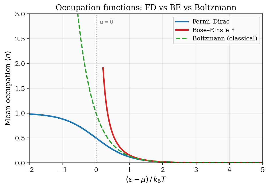
Figure 5: The three quantum occupation functions plotted versus \((\varepsilon-\mu)/k_{\rm B}T\). The Fermi–Dirac distribution is bounded between 0 and 1; the Bose–Einstein diverges as \(\varepsilon\to\mu^+\); both converge to the Maxwell–Boltzmann exponential for \(\varepsilon\gg\mu\).

Bosons wanting to bunch: exchange forces without a force

A striking quantum effect is that bosons attract each other statistically — they are more likely to be found in the same state than classical probability would predict — while fermions repel. This “exchange force” has no classical counterpart and arises purely from symmetrisation of the wave function.

To see this concretely, consider two non-interacting particles that can each occupy two states \(|1\rangle\) or \(|2\rangle\). The three cases — classical, bosonic, fermionic — give very different probabilities for finding both particles in the same state.

For classical distinguishable particles, the four configurations \((1,1)\), \((1,2)\), \((2,1)\), \((2,2)\) are each equally probable with probability \(1/4\). The probability of both particles being in the same state is \(2/4 = 1/2\).

For identical bosons, the distinct quantum states are \(|1\rangle|1\rangle\), \((|1\rangle|2\rangle + |2\rangle|1\rangle)/\sqrt{2}\), and \(|2\rangle|2\rangle\) — three states, each equally probable by the fundamental postulate. The probability of both particles in the same state is \(2/3 > 1/2\): bosons are more likely to be found together.

For identical fermions, only the antisymmetric combination \((|1\rangle|2\rangle - |2\rangle|1\rangle)/\sqrt{2}\) exists — a single state. Both particles are in the same state with probability \(0\): fermions cannot share a state. The Pauli exclusion principle is not a separate postulate — it is a consequence of antisymmetry.

The three probabilities — \(2/3\), \(1/2\), \(0\) — summarise the “exchange forces” for bosons, classical particles, and fermions respectively. These statistical correlations are pure quantum effects, present even for non-interacting particles, and they lead to dramatically different thermodynamic behaviours at low temperatures.

The non-degenerate limit: recovering Maxwell–Boltzmann

In the classical limit of high temperature and low density (\(n\lambda_{\rm dB}^3 \ll 1\)), both quantum distributions reduce to the Maxwell–Boltzmann result. We can see this from the grand canonical viewpoint. In this limit, the mean occupation of every mode is much less than 1: \(\langle n\rangle \ll 1\), which means \(e^{\beta(\varepsilon-\mu)} \gg 1\). The grand partition function for each mode then factorises as \(\mathcal{Z}_{\rm mode} \approx 1 + e^{-\beta(\varepsilon-\mu)}\) for both bosons and fermions (the distinction between \(\pm 1\) in the denominator is negligible). The total grand partition function for all modes factorises, and the mean occupation of mode \(\varepsilon\) is

\[ \langle n\rangle \approx e^{-\beta(\varepsilon-\mu)} = e^{\beta\mu}\, e^{-\beta\varepsilon}. \]

This is the Maxwell–Boltzmann Boltzmann factor with fugacity \(e^{\beta\mu}\). The condition \(\langle N\rangle = \sum_\varepsilon \langle n_\varepsilon\rangle = e^{\beta\mu}Z_1\) then fixes \(\mu = k_{\rm B}T\ln(N\lambda_{\rm dB}^3/V)\), exactly the ideal gas chemical potential from Chapter 6. The grand canonical approach thus provides a fully unified derivation of all three statistics and their classical limit.

The condition for quantum degeneracy can now be stated precisely. Define the phase-space occupancy \(\eta = n\lambda_{\rm dB}^3\). When \(\eta \ll 1\) the classical (Maxwell–Boltzmann) regime applies; when \(\eta \gtrsim 1\) quantum statistics are essential. For bosons, the threshold \(\eta \approx 2.612\) marks the BEC transition; for fermions, \(\eta \gtrsim 1\) marks the onset of Fermi degeneracy. As computed earlier: copper electrons have \(\eta \approx 5\) at room temperature (deeply degenerate Fermi gas); liquid \(^4\)He has \(\eta \approx 3\) at its normal boiling point (bosonic degeneracy, consistent with the superfluid transition); hydrogen gas at STP has \(\eta \approx 10^{-5}\) (classical). The phase-space occupancy \(\eta\) is the single most important dimensionless parameter in quantum statistical mechanics.

---

Chapter 8: Degenerate Fermi Gases and the Density of States

The Fermi sea at zero temperature

When temperature goes to zero with the particle number held fixed, the Fermi–Dirac distribution approaches a step function: every state with energy below the Fermi energy \(\varepsilon_{\rm F}\) is occupied (\(\langle n\rangle = 1\)) and every state above is empty (\(\langle n\rangle = 0\)). The Fermi energy is simply the chemical potential at \(T = 0\), determined by the requirement that the total number of particles equals the integral of the density of states over all occupied states.

The filled states form a Fermi sea in energy space. Unlike a classical gas, where all particles would rush to the ground state at \(T = 0\), fermions are forced by the Pauli exclusion principle to fill states one by one, all the way up to \(\varepsilon_{\rm F}\). This quantum pressure (which persists even at absolute zero) is responsible for the stability of metals, the rigidity of white dwarf stars, and the incompressibility of atomic nuclei.

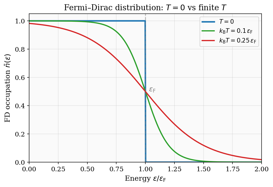
Figure 6: The Fermi–Dirac distribution at \(T=0\) (sharp step), \(k_{\rm B}T = 0.1\,\varepsilon_{\rm F}\), and \(k_{\rm B}T = 0.25\,\varepsilon_{\rm F}\). Thermal excitations smear the step over a window of width \(\sim k_{\rm B}T\) around the Fermi energy.

Density of states for a three-dimensional Fermi gas

To compute the Fermi energy and ground-state energy, we need the density of states \(g(\varepsilon)\), defined so that \(g(\varepsilon)\,d\varepsilon\) is the number of single-particle states with energy in \([\varepsilon, \varepsilon+d\varepsilon]\). For a particle in a 3D box of volume \(V\), the energy is \(\varepsilon = \hbar^2 k^2/2m\). We begin by counting states in \(k\)-space. Using periodic boundary conditions, the allowed \(\mathbf{k}\)-vectors form a cubic lattice with spacing \(2\pi/L\) in each direction, so the density of states in \(\mathbf{k}\)-space is \(V/(2\pi)^3\). The total number of states with wavevector magnitude less than \(k\), including the factor of 2 for electron spin, is

\[ N_{\rm states}(k) = 2\cdot\frac{V}{(2\pi)^3}\cdot\frac{4\pi k^3}{3} = \frac{V k^3}{3\pi^2}. \]

The density of states in energy is obtained by differentiating with respect to \(\varepsilon\) and using \(k = \sqrt{2m\varepsilon}/\hbar\), so \(dk/d\varepsilon = \sqrt{m/(2\hbar^2\varepsilon)}\):

\[ g(\varepsilon) = \frac{dN_{\rm states}}{d\varepsilon} = \frac{V k^2}{\pi^2}\frac{dk}{d\varepsilon} = \frac{V}{2\pi^2}\left(\frac{2m}{\hbar^2}\right)^{3/2}\sqrt{\varepsilon} \propto \varepsilon^{1/2}. \]

This \(\varepsilon^{1/2}\) density of states is the fundamental input to all Fermi gas calculations. Its form is entirely a consequence of three-dimensional geometry and the quadratic dispersion relation.

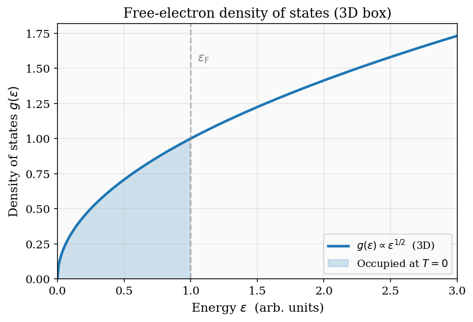
Figure 7: The free-electron density of states \(g(\varepsilon) \propto \varepsilon^{1/2}\) for a 3D box. The shaded region is occupied at \(T=0\); the Fermi energy \(\varepsilon_{\rm F}\) is the sharp cutoff.

Setting \(\int_0^{\varepsilon_{\rm F}} g(\varepsilon)\,d\varepsilon = N\) determines the Fermi energy:

\[ \varepsilon_{\rm F} = \frac{\hbar^2}{2m}\left(3\pi^2\,\frac{N}{V}\right)^{2/3}. \]

The Fermi energy of copper

For electrons in copper, the valence electron density is \(N/V \approx 8.5 \times 10^{28}\ \text{m}^{-3}\) (one conduction electron per copper atom, density \(8900\ \text{kg/m}^3\), atomic mass 63.5 u). Substituting \(m = m_e = 9.11\times 10^{-31}\ \text{kg}\) and \(\hbar = 1.055\times 10^{-34}\ \text{J s}\):

\[ \varepsilon_{\rm F} = \frac{(1.055\times 10^{-34})^2}{2(9.11\times 10^{-31})}\left(3\pi^2\times 8.5\times 10^{28}\right)^{2/3} \approx 7.0\ \text{eV}. \]

The Fermi temperature is \(T_{\rm F} = \varepsilon_{\rm F}/k_{\rm B} \approx 81{,}000\ \text{K}\). Room temperature is 300 K — a factor of 270 smaller than \(T_{\rm F}\). Copper’s conduction electrons are therefore profoundly quantum-mechanical at room temperature, with \(k_{\rm B}T/\varepsilon_{\rm F} \approx 0.004\). The classical equipartition prediction that each electron contributes \(\tfrac{3}{2}k_{\rm B}\) to the heat capacity is wildly wrong — the actual contribution is about 200 times smaller, suppressed by the Pauli exclusion principle as we quantify in Chapter 9.

Ground-state energy and degeneracy pressure

The total ground-state energy of the Fermi gas is obtained by integrating \(\varepsilon g(\varepsilon)\) up to \(\varepsilon_{\rm F}\):

\[ E_0 = \int_0^{\varepsilon_{\rm F}} \varepsilon\, g(\varepsilon)\,d\varepsilon = \frac{V}{2\pi^2}\left(\frac{2m}{\hbar^2}\right)^{3/2}\int_0^{\varepsilon_{\rm F}}\varepsilon^{3/2}\,d\varepsilon = \frac{V}{2\pi^2}\left(\frac{2m}{\hbar^2}\right)^{3/2}\frac{2\varepsilon_{\rm F}^{5/2}}{5} = \frac{3}{5}N\varepsilon_{\rm F}. \]

The average energy per electron is \(E_0/N = \tfrac{3}{5}\varepsilon_{\rm F} \approx 4.2\ \text{eV}\) for copper — much larger than the thermal energy \(k_{\rm B}T \approx 0.026\ \text{eV}\) at room temperature.

The corresponding zero-temperature degeneracy pressure follows from thermodynamics: for an ideal gas in any dimension, \(pV = \frac{2}{3}E\), so

\[ P_0 = \frac{2E_0}{3V} = \frac{2}{5}\frac{N}{V}\varepsilon_{\rm F}. \]

For copper, \(P_0 \approx 3.8\times 10^{10}\ \text{Pa} \approx 380{,}000\ \text{atm}\). This enormous pressure exists even at absolute zero and is entirely a quantum effect — the Pauli exclusion principle prevents the Fermi sea from collapsing. It is this degeneracy pressure that supports white dwarf stars against gravitational collapse.

White dwarf degeneracy pressure. A typical white dwarf has density \(\rho \sim 10^6\ \text{g/cm}^3 = 10^9\ \text{kg/m}^3\). Taking the composition to be primarily carbon-12 (6 protons + 6 neutrons + 6 electrons per nucleus), the electron number density is \(n_e \approx (6/12)\rho/m_p \approx (10^9)/(2\times 1.67\times 10^{-27}) \approx 3\times 10^{35}\ \text{m}^{-3}\). The corresponding Fermi energy is \(\varepsilon_{\rm F} \approx (\hbar^2/2m_e)(3\pi^2 n_e)^{2/3} \approx 0.2\ \text{MeV}\), which is comparable to \(m_e c^2 = 0.511\ \text{MeV}\) — electrons in a white dwarf are relativistic. The degeneracy pressure in the relativistic limit scales as \(P_0 \propto n_e^{4/3}\) rather than \(n_e^{5/3}\), and this softer scaling means that above a critical mass (\(\approx 1.4\ M_\odot\), the Chandrasekhar limit), the degeneracy pressure cannot balance gravity and the star collapses to a neutron star. The Chandrasekhar limit is a direct consequence of the relativistic correction to the Fermi degeneracy pressure.

---

Chapter 9: The Sommerfeld Expansion and Electrons in Metals

Low-temperature corrections to Fermi integrals

At finite temperature \(T \ll T_{\rm F} = \varepsilon_{\rm F}/k_{\rm B}\), the Fermi distribution is only slightly smeared compared to the sharp step at \(T = 0\). The mathematical tool that quantifies this smearing is the Sommerfeld expansion. For any smooth function \(h(\varepsilon)\),

\[ \int_0^\infty h(\varepsilon)\,\bar{n}_{\rm FD}(\varepsilon)\,d\varepsilon \approx \int_0^\mu h(\varepsilon)\,d\varepsilon + \frac{\pi^2}{6}(k_{\rm B}T)^2\,h'(\mu) + \cdots \]

The physical idea behind this expansion is that \(-\partial\bar{n}/\partial\varepsilon\) is sharply peaked at \(\varepsilon = \mu\), with a width of order \(k_{\rm B}T\). Integrating by parts, one can write \(\int h(\varepsilon)\bar{n}\,d\varepsilon = \int_0^\mu h(\varepsilon)\,d\varepsilon + \int_\mu^\infty h(\varepsilon)(-1)\bar{n}\,d\varepsilon + \ldots\), where the correction terms involve the derivatives of \(h\) at \(\varepsilon = \mu\). The key integral \(\int_0^\infty x^2/(e^x+e^{-x}+2)\,dx = \pi^2/6\) (a standard result, provable by contour integration or by the Euler–Maclaurin formula) produces the \(\pi^2/6\) coefficient of the leading correction.

Applying this to the constraint \(\int_0^\infty g(\varepsilon)\bar{n}_{\rm FD}(\varepsilon)\,d\varepsilon = N\) determines how the chemical potential shifts with temperature:

\[ \mu(T) \approx \varepsilon_{\rm F}\left[1 - \frac{\pi^2}{12}\left(\frac{k_{\rm B}T}{\varepsilon_{\rm F}}\right)^2\right]. \]

At room temperature in a metal, \(k_{\rm B}T/\varepsilon_{\rm F} \sim 0.004\), so \(\mu\) is within a fraction of a percent of \(\varepsilon_{\rm F}\). The chemical potential barely moves.

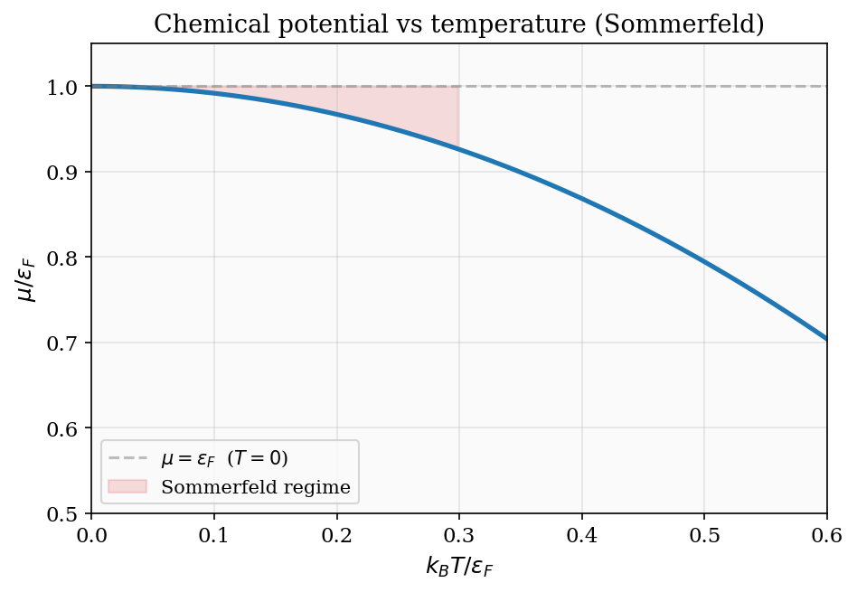
Figure 8: The chemical potential \(\mu(T)\) decreases quadratically from the Fermi energy as temperature rises. The shaded region marks the Sommerfeld regime \(k_{\rm B}T \ll \varepsilon_{\rm F}\) where the expansion is valid.

Electronic heat capacity

Applying the Sommerfeld expansion to the total energy gives the leading temperature correction:

\[ \langle E\rangle \approx E_0 + \frac{\pi^2}{6}(k_{\rm B}T)^2\,g(\varepsilon_{\rm F}). \]

The electronic heat capacity is therefore

\[ C_V^{\rm el} = \frac{\partial\langle E\rangle}{\partial T} = \frac{\pi^2}{3}k_{\rm B}^2 T\, g(\varepsilon_{\rm F}) = \gamma T, \qquad \gamma = \frac{\pi^2}{3}k_{\rm B}^2 g(\varepsilon_{\rm F}). \]

The linear-in-\(T\) dependence is the hallmark of a degenerate Fermi gas and has been confirmed in countless metals. Physically, only the fraction \(\sim k_{\rm B}T/\varepsilon_{\rm F}\) of electrons near the Fermi surface can absorb thermal energy (those deeper in the Fermi sea have no empty states nearby to jump into). This fraction, each absorbing \(\sim k_{\rm B}T\), gives \(C_V^{\rm el} \sim Nk_{\rm B} \cdot (k_{\rm B}T/\varepsilon_{\rm F})\), which is the same result up to factors of order unity.

At low temperatures in metals, the total heat capacity is \(C_V = \gamma T + AT^3\), where the \(AT^3\) contribution comes from lattice vibrations (the Debye model, discussed in Chapter 11). Measuring \(\gamma\) gives the electronic density of states at the Fermi level, which in turn encodes information about the band structure and electron-electron interactions.

Comparison with experiment

The Sommerfeld theory predicts a specific value of \(\gamma\) for each metal based on the free-electron density of states at \(\varepsilon_{\rm F}\): \(\gamma_{\rm free} = \pi^2 k_{\rm B}^2/2 \cdot g_{\rm free}(\varepsilon_{\rm F})\). Experimentally measured values often differ from this prediction, and the ratio \(\gamma_{\rm exp}/\gamma_{\rm free} \equiv m^*/m\) defines the effective mass enhancement. A few representative values:

Metal	\(\gamma_{\rm exp}\) (mJ mol\(^{-1}\) K\(^{-2}\))	\(\gamma_{\rm free}\)	\(m^*/m\)
Cu	0.70	0.50	1.38
Al	1.35	0.91	1.48
Au	0.73	0.64	1.14

The enhancement arises primarily from electron-phonon coupling: as an electron moves through the lattice, it drags a cloud of lattice distortion with it. This retardation effect makes the electron behave as if it were heavier than the bare electron mass, increasing the density of states at the Fermi level and thus \(\gamma\). In strongly correlated metals like heavy fermion compounds, \(m^*/m\) can reach \(10^2\)–\(10^3\), a dramatic manifestation of many-body physics.

The Wiedemann–Franz law

Both the electrical conductivity \(\sigma\) and the thermal conductivity \(\kappa\) of a metal are carried by electrons near the Fermi surface. The electrons travel a mean free path \(\ell\) between scattering events, and both conductivities depend on the same \(\ell\) and the same density of states \(g(\varepsilon_{\rm F})\). Dividing one by the other eliminates \(\ell\):

\[ \frac{\kappa}{\sigma} = L_0 T, \qquad L_0 = \frac{\pi^2 k_{\rm B}^2}{3e^2} \approx 2.44\times 10^{-8}\ \text{W}\,\Omega\,\text{K}^{-2}. \]

This is the Wiedemann–Franz law, and \(L_0\) is the Lorenz number. It is a universal prediction: the ratio \(\kappa/(\sigma T)\) should be the same for all metals, determined only by fundamental constants. The law holds to within 10–20% for most good metals at room temperature, confirming that both transport coefficients share the same microscopic origin — electrons at the Fermi surface.

Pauli paramagnetism

A magnetic field \(B\) shifts the energy of spin-up electrons by \(-\mu_{\rm B}B\) and spin-down electrons by \(+\mu_{\rm B}B\), where \(\mu_{\rm B} = e\hbar/2m_e\) is the Bohr magneton. At zero field, the spin-up and spin-down sub-bands are equally populated. The field unbalances this: it lowers the spin-up band, which gains electrons from the spin-down band until a new equilibrium is reached. The resulting magnetisation (excess spin-up electrons) is

\[ M = \mu_{\rm B}^2 B\, g(\varepsilon_{\rm F}). \]

This temperature-independent magnetisation is Pauli paramagnetism. It contrasts sharply with the Curie law \(M \propto 1/T\) of a classical paramagnet; the difference is precisely the Pauli exclusion principle suppressing the response of deeply buried electrons to the field.

To see this contrast clearly: a classical paramagnets has \(M = N\mu^2 B/3k_{\rm B}T\) (the factor of 3 from three-dimensional averaging of the classical dipole). For the quantum Fermi gas, only the \(N_{\rm eff} \sim Nk_{\rm B}T/\varepsilon_{\rm F}\) electrons near the Fermi surface can respond to the field; the rest are locked into filled states with no available adjacent empty state of opposite spin. Each contributing electron responds classically with \(\sim \mu_{\rm B}^2 B / k_{\rm B}T\), giving \(M \sim N_{\rm eff} \cdot \mu_{\rm B}^2 B/k_{\rm B}T \sim N\mu_{\rm B}^2 B/\varepsilon_{\rm F}\), which is the temperature-independent result above. The Pauli susceptibility \(\chi_{\rm Pauli} = \mu_{\rm B}^2 g(\varepsilon_{\rm F})\) is thus smaller than the Curie value by a factor \(\sim k_{\rm B}T/\varepsilon_{\rm F} \sim 0.004\) at room temperature in a metal — a dramatic suppression. Measuring \(\chi_{\rm Pauli}\) provides an independent determination of the density of states at the Fermi level, complementing the heat capacity measurement of \(\gamma\).

---

Chapter 10: Massless Bosons — Photons and the Planck Law

Photons as a Bose gas with \(\mu = 0\)

Electromagnetic radiation in thermal equilibrium with its surroundings — the interior of a hot furnace, the surface of a star, the early universe — is a gas of photons. Photons are spin-1 bosons, but they have a crucial distinguishing feature: their number is not conserved. A hot surface can emit or absorb any number of photons without violating any conservation law. This means that there is no constraint fixing the total number of photons, and the chemical potential is exactly zero: \(\mu_{\rm photon} = 0\). Setting \(\mu = 0\) in the Bose–Einstein distribution gives the mean occupation of a photon mode with energy \(\varepsilon = \hbar\omega\):

\[ \langle n\rangle = \frac{1}{e^{\hbar\omega/k_{\rm B}T} - 1}. \]

Photon density of states from first principles

The density of photon states in a cavity of volume \(V\) is derived by counting the electromagnetic modes. Using periodic boundary conditions, the allowed wave vectors \(\mathbf{k}\) form a cubic lattice with spacing \(2\pi/L\) in each direction, giving a density of states in \(\mathbf{k}\)-space of \(V/(2\pi)^3\) per unit \(k^3\)-volume. Each \(\mathbf{k}\) supports two independent polarisation states (two transverse polarisations; longitudinal modes do not propagate). The number of states with \(|\mathbf{k}|\) less than \(k\) is therefore

\[ N_{\rm states}(k) = 2\cdot\frac{V}{(2\pi)^3}\cdot\frac{4\pi k^3}{3} = \frac{Vk^3}{3\pi^2}. \]

Using the photon dispersion relation \(\varepsilon = \hbar\omega = \hbar ck\) (so \(k = \varepsilon/\hbar c\) and \(dk/d\varepsilon = 1/\hbar c\)):

\[ g(\varepsilon) = \frac{dN_{\rm states}}{d\varepsilon} = \frac{V k^2}{\pi^2}\frac{dk}{d\varepsilon} = \frac{V\varepsilon^2}{\pi^2\hbar^3 c^3}. \]

This is the photon density of states. The key difference from the massive-particle case is the linear dispersion \(\varepsilon \propto k\) (instead of \(\varepsilon \propto k^2\)), which gives \(g \propto \varepsilon^2\) (instead of \(\varepsilon^{1/2}\)).

The Planck spectrum

Multiplying the density of states by the mean occupation and the energy per mode, and dividing by \(V\), gives the spectral energy density:

\[ u(\varepsilon) = \frac{g(\varepsilon)}{V}\cdot\frac{\varepsilon}{e^{\varepsilon/k_{\rm B}T}-1} = \frac{\varepsilon^3}{\pi^2\hbar^3 c^3}\cdot\frac{1}{e^{\varepsilon/k_{\rm B}T}-1}. \]

This is the Planck distribution, derived by Planck in 1900 (though his derivation proceeded differently). It is the unique spectral distribution for blackbody radiation in thermal equilibrium.

The classical Rayleigh–Jeans limit and the ultraviolet catastrophe

In the classical limit of high temperature (\(\hbar\omega \ll k_{\rm B}T\)), the exponential in the denominator expands as \(e^{\hbar\omega/k_{\rm B}T} - 1 \approx \hbar\omega/k_{\rm B}T\), so the Planck distribution becomes

\[ u(\varepsilon) \approx \frac{\varepsilon^2}{\pi^2\hbar^3 c^3}\cdot k_{\rm B}T = \frac{\omega^2 k_{\rm B}T}{\pi^2 c^3}. \]

This is the Rayleigh–Jeans law. It agrees with the classical equipartition theorem: each electromagnetic mode with frequency \(\omega\) is a harmonic oscillator with average energy \(k_{\rm B}T\) (electric and magnetic fields each contributing \(\tfrac{1}{2}k_{\rm B}T\)). The problem is that the Rayleigh–Jeans formula diverges as \(\omega^2\) without bound — integrating over all frequencies gives an infinite total energy density. This is the ultraviolet catastrophe: classically, a blackbody should radiate infinite energy. Planck’s resolution — that electromagnetic energy is quantised in units of \(\hbar\omega\) — suppresses the high-frequency modes via the exponential \(e^{\hbar\omega/k_{\rm B}T}\), producing the observed finite spectrum.

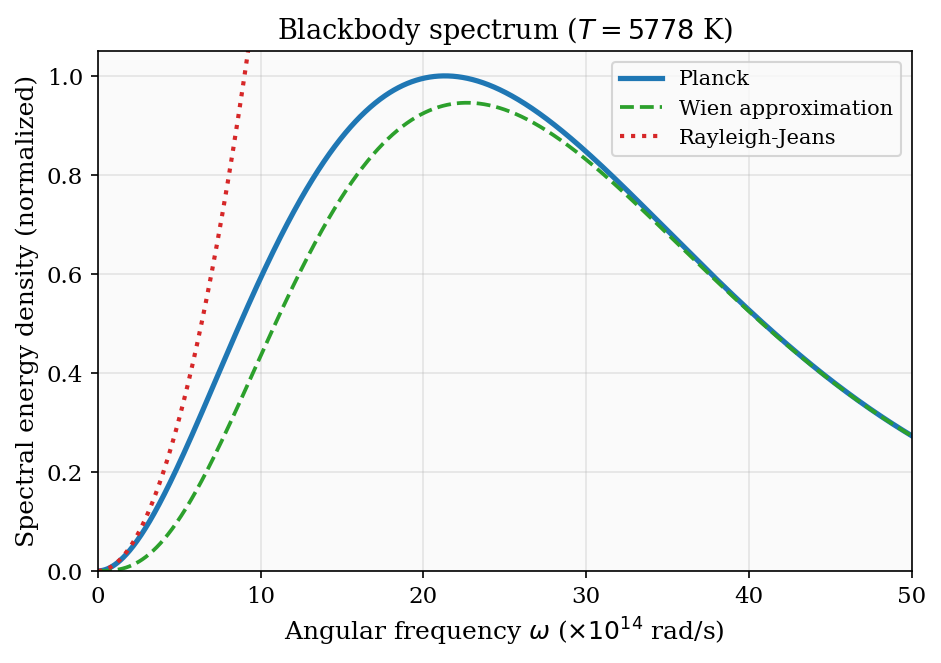
Figure 9: The Planck spectrum (solid) at solar surface temperature \(\approx 5778\ \text{K}\). The Wien approximation (dashed) works well at high frequency; the Rayleigh–Jeans law (dotted) works at low frequency but diverges at high frequency — the “ultraviolet catastrophe” that Planck’s quantisation resolved.

Wien’s law and Stefan–Boltzmann

Differentiating \(u(\varepsilon)\) with respect to \(\varepsilon\) and setting the result to zero gives the energy of the spectral peak:

\[ \varepsilon_{\rm peak} \approx 2.82\,k_{\rm B}T \qquad \Rightarrow\qquad \lambda_{\rm peak} T = 2.898 \times 10^{-3}\ \text{m K}. \]

This is Wien’s displacement law: the peak wavelength is inversely proportional to temperature.

The Stefan–Boltzmann law

The total energy density of blackbody radiation is obtained by integrating the Planck spectrum over all energies. Changing variables to \(x = \varepsilon/k_{\rm B}T\):

\[ u_{\rm total} = \int_0^\infty u(\varepsilon)\,d\varepsilon = \frac{(k_{\rm B}T)^4}{\pi^2\hbar^3 c^3}\int_0^\infty \frac{x^3}{e^x-1}\,dx. \]

The dimensionless integral is a standard result: \(\int_0^\infty x^3/(e^x-1)\,dx = \pi^4/15\) (provable using the Riemann zeta function \(\zeta(4) = \pi^4/90\) and the relation \(\int_0^\infty x^3/(e^x-1)\,dx = 6\zeta(4)\)). Therefore \(u_{\rm total} = (\pi^2/15)(k_{\rm B}T)^4/(\hbar^3 c^3)\), giving a total energy that scales as \(T^4\).

The power radiated per unit area by a blackbody surface is \(j = cu_{\rm total}/4\) (the factor of \(c/4\) comes from integrating the flux over the hemisphere, analogous to the effusion formula \(\Phi = n\langle v\rangle/4\)). This gives the Stefan–Boltzmann law:

\[ j = \sigma T^4, \qquad \sigma = \frac{2\pi^5 k_{\rm B}^4}{15 h^3 c^2} \approx 5.67 \times 10^{-8}\ \text{W m}^{-2}\text{K}^{-4}. \]

Stellar luminosity

For a star of radius \(R\) and surface temperature \(T\), the total luminosity is

\[ L = 4\pi R^2 \sigma T^4. \]

For the Sun, \(R_\odot = 6.96\times 10^8\ \text{m}\) and \(T_\odot \approx 5778\ \text{K}\), giving

\[ L_\odot = 4\pi(6.96\times 10^8)^2(5.67\times 10^{-8})(5778)^4 \approx 3.83\times 10^{26}\ \text{W}, \]

in excellent agreement with the measured solar luminosity. This relationship underlies the Hertzsprung–Russell diagram: stars of different temperatures and radii lie along sequences determined by \(L \propto R^2 T^4\). The main sequence corresponds to stars with hydrogen-burning cores, where the radius and temperature are tightly correlated by stellar structure equations. Red giants are cool (\(T \sim 3000\ \text{K}\)) but luminous (\(L \sim 10^3 L_\odot\)) because of their enormous radii; blue supergiants are hot and bright. The HR diagram is essentially a display of the Stefan–Boltzmann law for the stellar population.

Wien’s displacement law applications

Wien’s displacement law \(\lambda_{\rm peak}T = 2.898\times 10^{-3}\ \text{m K}\) has a remarkable range of applications. The Sun’s surface at \(5778\ \text{K}\) peaks at \(\lambda \approx 502\ \text{nm}\) — green light. Human eyes evolved their peak sensitivity near 555 nm, closely matching this peak and giving us an intuitive feel for solar colour. A human body at \(310\ \text{K}\) peaks at \(\lambda \approx 9.4\ \mu\text{m}\) — mid-infrared, invisible to the eye but detectable by thermal cameras (useful for medical thermography and night-vision goggles). A stellar remnant neutron star with surface temperature \(T \sim 10^6\ \text{K}\) peaks at \(\lambda \sim 3\ \text{nm}\) — in the soft X-ray band, exactly where neutron star emission is observed by X-ray telescopes.

Wien’s law also gives a quick way to estimate stellar surface temperatures from colour. A star that appears red has \(\lambda_{\rm peak} \gtrsim 700\ \text{nm}\), implying \(T \lesssim 4000\ \text{K}\); a blue star has \(\lambda_{\rm peak} \lesssim 400\ \text{nm}\), implying \(T \gtrsim 7250\ \text{K}\). The HR diagram’s colour-temperature correlation is nothing more than Wien’s displacement law applied to stars.

The cosmic microwave background

Perhaps the most spectacular confirmation of the Planck spectrum is the cosmic microwave background (CMB). The universe at early times was a dense, hot plasma opaque to radiation; photons and matter were in thermal equilibrium. As the universe expanded and cooled to about \(3000\ \text{K}\), hydrogen recombined and the universe became transparent. The photons have been streaming freely ever since, but redshifted by the expansion to an effective temperature of \(T_{\rm CMB} = 2.725\ \text{K}\). The COBE satellite’s FIRAS instrument measured the CMB spectrum to be a perfect blackbody to one part in \(10^4\) — the most perfect blackbody spectrum ever measured.

The nearly perfect blackbody spectrum of the CMB provides powerful cosmological constraints. The tiny deviations from a perfect blackbody — at the level of one part in \(10^5\) — encode information about chemical processes in the early universe (Compton scattering efficiency, energy injection from possible exotic particles). The spatial temperature fluctuations of the CMB (anisotropies at the level of \(10^{-5}\)) encode the seeds of large-scale structure — the density perturbations that grew into galaxies and galaxy clusters. Analysing these anisotropies with the power spectrum of the CMB has become one of the most powerful probes of cosmological parameters. The fact that all of this rich cosmological information rides on the back of a blackbody spectrum — derivable from the Planck distribution we found in this chapter — is a striking illustration of how foundational statistical mechanics is to our understanding of the universe.

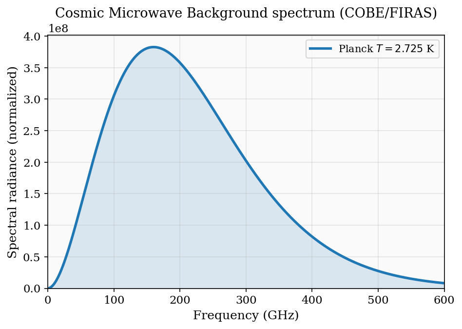
Figure 10: The CMB blackbody spectrum at \(T = 2.725\ \text{K}\). The COBE/FIRAS measurement matches the Planck distribution so precisely that error bars are smaller than the line width in most plots.

---

Chapter 11: The Debye Model of Phonons

Normal modes and phonons

A solid with \(N\) atoms has \(3N\) degrees of freedom: three displacement directions for each atom. When the atoms are arranged in a crystal, the equations of motion for small displacements from equilibrium can be diagonalised to give \(3N\) normal modes of vibration, each characterised by a wavevector \(\mathbf{k}\) and a polarisation. Each normal mode is mathematically a quantum harmonic oscillator with a mode-specific frequency \(\omega_\mathbf{k}\). The quantised energy quanta of these oscillators are phonons — quasiparticles that carry energy \(\hbar\omega\), are bosons (integer spin), have zero chemical potential (phonon number is not conserved; the lattice can emit or absorb phonons freely), and obey the Planck distribution. Phonons in a solid are directly analogous to photons in a radiation field: both are massless bosons with \(\mu = 0\), the difference being that photons have a linear dispersion \(\omega = ck\) for all \(k\), while phonons have a linear dispersion \(\omega = c_s k\) only for small \(k\) (the acoustic branch), with the dispersion becoming flat near the Brillouin zone boundary.

The Einstein and Debye models

The Einstein model of a solid treats each atom as an independent harmonic oscillator with a single frequency \(\omega_E\). The heat capacity at constant volume predicted by this model is

\[ C_V^{\rm Einstein} = 3Nk_{\rm B}\,\frac{(\beta\hbar\omega_E)^2\,e^{\beta\hbar\omega_E}}{(e^{\beta\hbar\omega_E}-1)^2}. \]

At high temperatures (\(k_{\rm B}T \gg \hbar\omega_E\)), this correctly approaches the Dulong–Petit value \(3Nk_{\rm B}\). At low temperatures, however, the Einstein model gives an exponential decay \(C_V \propto e^{-\hbar\omega_E/k_{\rm B}T}\), whereas experiments on real solids show a power-law \(C_V \propto T^3\). The Einstein model fails at low temperatures because it assumes all atoms vibrate at the same frequency, whereas a real crystal has a spectrum of normal modes ranging from zero frequency (long-wavelength acoustic phonons) to some cutoff frequency.

The Debye model corrects this by treating the solid as an elastic continuum with a linear dispersion relation \(\omega = c_s k\). The density of phonon states for acoustic modes is \(g(\omega) \propto \omega^2\), matching the photon case (with \(c\) replaced by the speed of sound \(c_s\) and including three polarisations — one longitudinal and two transverse). We integrate up to a maximum Debye frequency \(\omega_D\) chosen to give the correct total number of modes:

\[ \int_0^{\omega_D} g(\omega)\,d\omega = 3N \quad \Rightarrow \quad g(\omega) = \frac{9N\omega^2}{\omega_D^3}. \]

This fixes \(\omega_D\) in terms of the atomic density and speed of sound: \(\omega_D = c_s(6\pi^2 N/V)^{1/3}\). The associated Debye temperature is \(\Theta_D = \hbar\omega_D/k_{\rm B}\).

Phonons are massless bosons with \(\mu = 0\), so their mean occupation is the Planck distribution with \(\varepsilon = \hbar\omega\). The total energy of the solid is

\[ \langle E\rangle = \int_0^{\omega_D} \frac{\hbar\omega}{e^{\hbar\omega/k_{\rm B}T}-1}\,g(\omega)\,d\omega = 9Nk_{\rm B}T\left(\frac{T}{\Theta_D}\right)^3\int_0^{\Theta_D/T}\frac{x^3}{e^x-1}\,dx, \]

where we have changed variables to \(x = \hbar\omega/k_{\rm B}T\). The heat capacity \(C_V = \partial\langle E\rangle/\partial T\) involves the temperature derivative of this integral.

The low-temperature \(T^3\) law

At low temperature (\(T \ll \Theta_D\)), the upper limit of the integral \(\Theta_D/T \to \infty\). The Planck factor \(1/(e^x-1)\) decays exponentially for \(x \gg 1\), so the integrand is negligibly small long before \(x = \Theta_D/T\) — we can extend the upper limit to infinity with exponentially small error:

\[ \int_0^{\Theta_D/T}\frac{x^3}{e^x-1}\,dx \approx \int_0^\infty\frac{x^3}{e^x-1}\,dx = \frac{\pi^4}{15}. \]

The total energy is then \(\langle E\rangle = 9Nk_{\rm B}T(\pi^4/15)(T/\Theta_D)^3 = (3\pi^4/5)Nk_{\rm B}T(T/\Theta_D)^3\), and differentiating:

\[ C_V = \frac{12\pi^4}{5}Nk_{\rm B}\left(\frac{T}{\Theta_D}\right)^3. \]

This is the celebrated Debye \(T^3\) law, in excellent agreement with experiment at low temperatures. The numerical prefactor \(12\pi^4/5 \approx 234\) is a precise prediction with no free parameters (once \(\Theta_D\) is fixed from the high-temperature fit).

Debye temperatures and material properties

Material	\(\Theta_D\) (K)	Bonding character
Pb	88	metallic, weak
Na	158	metallic
Cu	343	metallic
Al	428	metallic
Fe	470	metallic
Si	645	covalent
Diamond	1860	covalent, stiff

Stiffer materials (stronger bonds, lighter atoms) have higher Debye temperatures. Diamond, with its extremely stiff carbon-carbon covalent bonds and low atomic mass, has \(\Theta_D \approx 1860\ \text{K}\). This means that at room temperature, \(T/\Theta_D \approx 0.16\) — diamond is not yet in the Dulong–Petit regime, which is why its heat capacity is much less than \(3Nk_{\rm B}\) at room temperature (indeed, the anomalously small heat capacity of diamond was one of the historical puzzles that motivated Einstein’s model). The Debye \(T^3\) law holds for \(T \lesssim \Theta_D/10\), so for diamond this requires \(T \lesssim 186\ \text{K}\). However, in practice the \(T^3\) regime is only cleanly visible below \(T \lesssim \Theta_D/50 \sim 37\ \text{K}\), because higher-order corrections become significant nearer to \(\Theta_D/10\). Observing pure \(T^3\) behaviour in diamond requires sub-50 K measurements.

Why Debye gives \(T^3\) while Einstein gives \(e^{-\Theta_E/T}\)

The physical reason for the difference is the acoustic gap: the Einstein model has a fixed frequency \(\omega_E\), and at temperatures \(k_{\rm B}T < \hbar\omega_E\) there is not enough thermal energy to excite even one quantum of vibration. Excitation is therefore exponentially suppressed, exactly as for the two-level system Schottky anomaly discussed in Chapter 3.

The Debye model, by contrast, has acoustic modes with \(\omega\to 0\) as \(k\to 0\). There is no energy gap — you can always excite a very-long-wavelength acoustic mode with arbitrarily little energy. At low temperature, only these low-frequency modes (\(\hbar\omega \lesssim k_{\rm B}T\)) contribute, and the density of states \(g(\omega) \propto \omega^2\) means there are few of them. The number of thermally excited modes scales as \(\omega_{\rm max}^3 \propto T^3\), each carrying energy \(\sim k_{\rm B}T\), giving total energy \(\propto T^4\) and heat capacity \(\propto T^3\). The \(T^3\) is a power law, not an exponential — it never reaches zero as fast as an exponential, but it never has a gap either. This is why the Debye \(T^3\) law works at low temperatures in all crystalline solids.

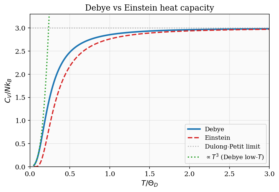
Figure 11: Heat capacity per atom in units of \(k_{\rm B}\) for the Debye model (solid), the Einstein model (dashed), and the Dulong–Petit plateau (dotted). At low \(T/\Theta_D\), the Debye model’s \(T^3\) tail (dotted green) matches experiment while Einstein’s exponential decay does not.

---

Chapter 12: Massive Bosons and Bose–Einstein Condensation

The chemical potential cannot exceed the ground-state energy

For a gas of \(N\) non-relativistic bosons with a conserved particle number, the chemical potential is determined by the constraint \(\langle N\rangle = \int_0^\infty g(\varepsilon)\bar{n}_{\rm BE}(\varepsilon)\,d\varepsilon = N\). The Bose–Einstein mean occupation \(\bar{n}_{\rm BE} = 1/(e^{\beta(\varepsilon-\mu)}-1)\) is positive only when \(\mu < \varepsilon\), and it diverges as \(\varepsilon\to\mu^+\). This divergence is not a pathology — it is a signal. As \(\mu\) approaches the ground-state energy \(\varepsilon_{\rm min} = 0\) from below, the occupation of the ground-state mode becomes

\[ \langle n_0\rangle = \frac{1}{e^{-\beta\mu}-1} \approx \frac{k_{\rm B}T}{|\mu|} \to \infty \quad \text{as } \mu\to 0^-. \]

The ground state is on the verge of macroscopic occupation. For classical statistics, the occupation of any single mode is of order \(N/\Omega \ll 1\) where \(\Omega\) is the number of accessible states — vanishingly small in the thermodynamic limit. For bosons near \(\mu = 0\), the ground state alone can accommodate a macroscopic number \(N_0 = O(N)\) of particles. This is the essence of BEC.

As the temperature is lowered, \(\mu\) must rise toward 0 to accommodate the fixed particle number. The question is: what happens when \(\mu \to 0^-\) and the integral over excited states reaches its maximum?

The condensation temperature

The integral \(\int_0^\infty g(\varepsilon)/(e^{\beta\varepsilon}-1)\,d\varepsilon\) (evaluated with \(\mu = 0\)) with the 3D density of states \(g(\varepsilon) \propto \varepsilon^{1/2}\) can be evaluated by the substitution \(x = \beta\varepsilon\):

\[ \int_0^\infty \frac{g(\varepsilon)}{e^{\beta\varepsilon}-1}\,d\varepsilon = \frac{V}{2\pi^2}\left(\frac{2m}{\hbar^2}\right)^{3/2}\int_0^\infty \frac{\varepsilon^{1/2}}{e^{\beta\varepsilon}-1}\,d\varepsilon = \frac{V}{\lambda_{\rm dB}^3}\cdot\frac{2}{\sqrt{\pi}}\int_0^\infty\frac{x^{1/2}}{e^x-1}\,dx. \]

The dimensionless integral is related to the Riemann zeta function by \(\int_0^\infty x^{1/2}/(e^x-1)\,dx = \Gamma(3/2)\zeta(3/2) = (\sqrt{\pi}/2)\zeta(3/2)\), where \(\zeta(3/2) \approx 2.612\). Therefore the maximum number of particles that the excited states can accommodate at temperature \(T\) is

\[ N_{\rm excited}^{\rm max} = \frac{V}{\lambda_{\rm dB}^3}\cdot\zeta(3/2) \approx 2.612\,\frac{V}{\lambda_{\rm dB}^3}. \]

When the temperature drops below the condensation temperature \(T_c\) defined by

\[ N = 2.612\,\frac{V}{\lambda_{\rm dB}^3(T_c)} \qquad \Rightarrow \qquad k_{\rm B}T_c = \frac{2\pi\hbar^2}{m}\left(\frac{N}{2.612\,V}\right)^{2/3}, \]

the excited states can no longer accommodate all \(N\) particles. The surplus particles must go somewhere: they condense into the single-particle ground state \(\varepsilon = 0\). This is Bose–Einstein condensation (BEC).

The number of particles in the ground state (the condensate fraction) for \(T < T_c\) is

\[ \frac{N_0}{N} = 1 - \left(\frac{T}{T_c}\right)^{3/2}. \]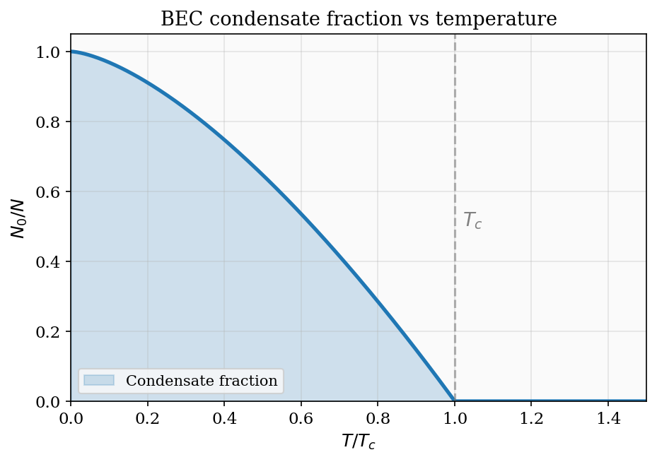

Figure 12: The condensate fraction \(N_0/N = 1-(T/T_c)^{3/2}\) (blue) and the thermal fraction occupying excited states (unshaded). At \(T_c\) the entire population is thermal; below \(T_c\) a macroscopic fraction occupies the ground state.

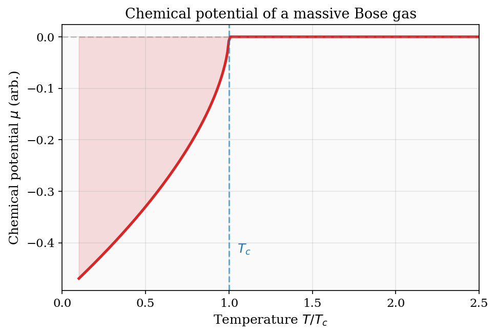
Figure 13: The chemical potential of a massive Bose gas approaches zero from below as \(T\to T_c^-\), then remains at \(\mu = 0\) in the condensed phase.

Heat capacity of a BEC

Below \(T_c\), the condensate (particles in the \(\varepsilon = 0\) ground state) contributes nothing to the heat capacity: they are all in a single state and have no entropy. All thermodynamic response comes from the excited fraction \(N_{\rm ex} = N(T/T_c)^{3/2}\). The total energy of the excited atoms scales as \(E \propto T^{5/2}\) (from the same integral as above, now weighted by \(\varepsilon\)), so the heat capacity below \(T_c\) scales as

\[ C_V \propto T^{3/2} \quad (T < T_c). \]

More precisely, \(C_V = (15/4)\zeta(5/2)/\zeta(3/2) \cdot Nk_{\rm B}(T/T_c)^{3/2}\) where \(\zeta(5/2)\approx 1.341\). Above \(T_c\), the heat capacity decreases from its value at \(T_c^+\) and eventually approaches the classical ideal-gas value \(\tfrac{3}{2}Nk_{\rm B}\). The heat capacity therefore has a cusp at \(T_c\) — a discontinuity in its slope — which is the thermodynamic signature of the BEC phase transition. This cusp (and the associated lambda-shaped specific heat curve) is analogous to the \(\lambda\)-transition observed in liquid helium-4.

The \(T^{3/2}\) scaling of the heat capacity below \(T_c\) is worth comparing with other systems. The Debye phonon heat capacity goes as \(T^3\), the Fermi liquid heat capacity goes as \(T\), and the BEC heat capacity goes as \(T^{3/2}\). Each power law reflects the dimensionality of the relevant excitation spectrum. Phonons in 3D have a density of states \(g(\omega) \propto \omega^2\) and dispersion \(\omega \propto k\), giving \(T^3\). Fermi liquid excitations are concentrated at the Fermi surface (a 2D object in 3D \(k\)-space), giving \(T\). BEC excitations occupy the 3D \(\varepsilon^{1/2}\) density of states with chemical potential \(\mu = 0\), giving \(T^{3/2}\). In each case the power law is determined by the phase space of thermally accessible excitations, and that phase space is controlled by the dispersion relation and the dimensionality of the system.

Superfluid helium-4 and the limitations of the ideal BEC theory

Liquid \(^4\)He undergoes a phase transition at \(T_\lambda = 2.17\ \text{K}\), below which it becomes a superfluid — a phase with zero viscosity, quantised vortices, and the ability to climb up container walls (the fountain effect). The transition was historically identified as a BEC of helium-4 atoms, and the temperature \(T_\lambda\) is close to the ideal-gas BEC prediction \(T_c\) based on the liquid helium number density.

However, helium is a liquid, not a dilute gas, and inter-atomic interactions are strong. One consequence is that only about \(8\%\) of helium atoms occupy the single-particle ground state at \(T = 0\), in stark contrast to the ideal-gas BEC where \(N_0/N \to 1\) at \(T = 0\). The remaining atoms are depleted from the condensate by quantum fluctuations driven by the interatomic interactions. The superfluid properties (zero viscosity, phase coherence) are nevertheless present because the condensate fraction, though small, still possesses long-range phase coherence. This example shows that BEC and superfluidity are related but not identical concepts: BEC is about macroscopic occupation of a single quantum state, while superfluidity is about the rigidity of the macroscopic quantum phase.

The low-temperature heat capacity of superfluid \(^4\)He scales as \(T^3\) rather than the ideal BEC’s \(T^{3/2}\). This is because the dominant low-energy excitations in superfluid helium are phonons (longitudinal density waves, acoustic modes of the liquid), not free-particle excitations. Landau showed that the spectrum of excitations in superfluid helium consists of phonons at low wavevector (\(\omega \propto k\), giving \(T^3\) Debye-like heat capacity) and rotons near a wavevector \(k_0 \approx 1.9\ \text{\AA}^{-1}\) (a local minimum in the dispersion relation, giving exponentially activated contributions). The phonon-roton spectrum, confirmed by neutron scattering, is the definitive experimental fingerprint of superfluidity in helium-4 and has no counterpart in the ideal Bose gas. The gap between the ideal BEC and the real superfluid is bridged by the Bogoliubov theory of weakly interacting bosons, which shows that even a small repulsive interaction converts the quadratic single-particle dispersion \(\varepsilon \propto k^2\) into a linear phonon dispersion at low \(k\), with profound consequences for the thermodynamics and the superfluid properties.

Interpreting the condensation

BEC is qualitatively different from ordinary phase transitions. The condensate does not form because of inter-particle attractions (unlike liquid-gas condensation); it forms because of quantum statistics alone — the Bose bunching tendency, which at high enough phase-space density (\(n\lambda_{\rm dB}^3 \gtrsim 2.612\)) forces macroscopic occupation of the single lowest-energy state. Bose and Einstein predicted this condensation in 1924–25. It took seventy years to observe it directly in the lab, because achieving the required phase-space density in a dilute gas requires cooling to temperatures of order \(100\ \text{nK}\). The techniques that made this possible are the subject of the next chapter.

The BEC transition can be understood as a kind of saturation phenomenon. The excited states of the ideal Bose gas can hold only a finite number of particles at a given temperature — once the temperature is lowered below \(T_c\), the extra particles have no choice but to pile into the ground state. This is fundamentally different from the Fermi case: at any temperature, one can always add more fermions because there are always unoccupied states (above the Fermi level). Bosons, by contrast, become “full” — the excited states saturate, and the overflow populates the condensate. The condensate is therefore not just the ground state being cold; it is a consequence of the Bose–Einstein statistics enforcing macroscopic coherence when the occupation number of the lowest mode diverges. This is why the condensate possesses off-diagonal long-range order (ODLRO), a concept introduced by Penrose and Onsager to characterise superfluidity and superconductivity in a unified framework: the one-body density matrix \(\rho(\mathbf{r}, \mathbf{r}') = \langle\Psi^\dagger(\mathbf{r})\Psi(\mathbf{r}')\rangle\) has a nonzero limit as \(|\mathbf{r} - \mathbf{r}'|\to\infty\) for \(T < T_c\), reflecting the long-range phase coherence of the condensate. ODLRO is absent in classical and normal quantum gases.

---

Chapter 13: BEC in the Laboratory

Trapping and cooling neutral atoms

To observe BEC in a dilute atomic gas, one must simultaneously achieve an extremely low temperature (nanokelvin regime) and a high enough density that the phase-space density exceeds the condensation threshold. The two principal tools are laser cooling and trapping, which bring atoms to temperatures of order \(10\ \mu\text{K}\), followed by evaporative cooling in a conservative trap, which drives the gas below \(T_c\).

Laser cooling exploits the Doppler effect and the momentum carried by photons. Consider an atom moving with velocity \(v\) toward a laser beam propagating in the \(-\hat{x}\) direction, tuned slightly below the atomic resonance frequency \(\omega_0\). In the atom’s rest frame, the laser frequency is blue-shifted by the Doppler effect to \(\omega_{\rm laser}(1 + v/c)\), bringing it closer to resonance. The atom preferentially absorbs photons from this beam (gaining momentum \(-\hbar k\) per photon) and then re-emits spontaneously in a random direction. Over many cycles, the net effect is a velocity-dependent drag force \(F = -\alpha v\), slowing the atom. The minimum temperature achievable by this mechanism — the Doppler cooling limit — is set by the balance between the cooling force and the random momentum kicks from spontaneous emission:

\[ k_{\rm B}T_{\rm Doppler} = \frac{\hbar\Gamma}{2}, \]

where \(\Gamma\) is the natural linewidth (spontaneous emission rate) of the atomic transition. For the sodium D line with \(\Gamma/(2\pi) \approx 9.8\ \text{MHz}\), this gives \(T_{\rm Doppler} \approx 240\ \mu\text{K}\). Six laser beams (two for each spatial direction) create an optical molasses that damps motion in all directions.

Sub-Doppler cooling techniques, discovered shortly after Doppler cooling, use the spatial variation of the polarisation gradient of the laser field to cool atoms below the Doppler limit. In Sisyphus cooling, atoms moving through a spatially periodic polarisation pattern climb potential hills created by the light-shift (AC Stark shift), losing kinetic energy on each hill climb. At the top of each hill, the atoms are optically pumped to the bottom of the next hill, and the process repeats. Sisyphus cooling can reach temperatures of order \(T_{\rm rec} = \hbar^2 k^2/(2mk_{\rm B})\) — the recoil temperature, a few \(\mu\text{K}\) — limited only by the random recoil from individual photon absorptions.

Magnetic trapping is the next stage. A magnetic trap exploits the force \(\mathbf{F} = \nabla(\boldsymbol{\mu}_{\rm atom}\cdot\mathbf{B})\) on an atom with a magnetic dipole moment \(\boldsymbol{\mu}_{\rm atom}\). Atoms in a weak-field-seeking state (magnetic moment anti-aligned with \(\mathbf{B}\)) are attracted to the minimum of the magnetic field magnitude. Earnshaw’s theorem from classical electrostatics (no local maximum of \(|\mathbf{B}|\) in free space) implies that strong-field-seeking states cannot be trapped statically, so only weak-field-seeking states are magnetically trappable. The Ioffe–Pritchard geometry — a set of four bar magnets or wires providing a radial quadrupole field plus bias coils for the axial confinement — is the most commonly used geometry, creating a harmonic trap with a non-zero field minimum (preventing Majorana spin-flip losses at the centre).

Evaporative cooling is the decisive step. The trapping field is modified (by radio-frequency magnetic fields that spin-flip atoms at a specific field value, selecting atoms at a specific energy) to selectively remove the most energetic atoms. After each removal step, the remaining atoms rethermalise by elastic collisions to a lower temperature. Repeating this process can cool a gas by many orders of magnitude in temperature at the cost of losing perhaps \(90\%\) of the atoms. The key figure of merit is the phase-space density \(n\lambda_{\rm dB}^3\), which increases even as the atom number decreases, because \(T\) drops faster than \(n\).

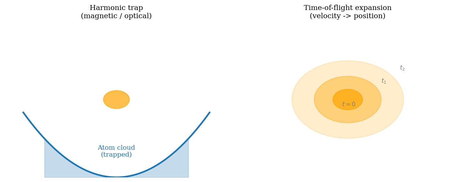
Figure 14: Left: atoms confined in a harmonic magnetic trap (parabolic potential, orange dot = cloud). Right: three time-of-flight snapshots after the trap is switched off. The cloud expands at a rate proportional to its velocity distribution, mapping momentum space to position space.

Time-of-flight imaging and the BEC signature

The standard technique for observing BEC is time-of-flight (TOF) absorption imaging. The confining trap is switched off suddenly, and the atom cloud expands freely. After a flight time \(t\), the density distribution at position \(\mathbf{r}\) reflects the original momentum distribution: atoms with momentum \(\mathbf{p}\) have travelled a distance \(\mathbf{r} = \mathbf{p}\,t/m\). The relationship between the post-flight density profile and the original momentum distribution is thus

\[ n_{\rm TOF}(\mathbf{r}, t) = n_{\rm momentum}\!\left(\frac{m\mathbf{r}}{t}\right)\cdot\left(\frac{m}{t}\right)^3. \]

A resonant laser beam passing through the expanded cloud is absorbed in proportion to the column density, casting a shadow on a CCD camera. This absorption image maps out the projected (integrated along the beam) density.

Above \(T_c\), the thermal cloud expands isotropically with a Gaussian profile reflecting the Maxwell–Boltzmann momentum distribution — a spherically symmetric density in momentum space produces a spherically symmetric density in the TOF image. Below \(T_c\), the condensate expands anisotropically. The condensate wave function in a harmonic trap \(V = \frac{1}{2}m(\omega_x^2 x^2 + \omega_y^2 y^2 + \omega_z^2 z^2)\) has a narrower spatial extent in the tightly confined direction. After release, the condensate expands faster in the tight direction (larger momentum spread due to Heisenberg uncertainty) and slower in the loose direction. After a long TOF, the aspect ratio inverts: a cigar-shaped cloud (tight in one direction) becomes a pancake (wide in the formerly tight direction). This inversion of the aspect ratio is a unique signature of BEC — a thermal cloud always expands isotropically regardless of the trap shape, because the Maxwell–Boltzmann distribution in momentum space is always spherically symmetric.

The bimodal density profile — a sharp, anisotropic condensate peak sitting on a broad, isotropic thermal halo — was the definitive experimental signature seen by the JILA group (Anderson et al., 1995) in \(^{87}\)Rb and almost simultaneously by the MIT group (Davis et al., 1995) in \(^{23}\)Na. The Nobel Prize in Physics 2001 was awarded to Cornell, Wieman, and Ketterle for this achievement.

Matter-wave coherence and interference

A Bose–Einstein condensate is not merely a very cold gas. All the condensate atoms occupy the same single-particle quantum state, described by a macroscopic wave function (or order parameter) \(\Psi(\mathbf{r})\), normalised so that \(|\Psi(\mathbf{r})|^2 = n_0(\mathbf{r})\) is the condensate density.

If two BECs are prepared in neighbouring potential wells and then allowed to overlap, they interfere — producing a spatially periodic fringe pattern. This matter-wave interference (first seen by Andrews et al., MIT 1997) is direct evidence that the condensate is a coherent quantum state.

Superfluidity and the macroscopic wave function

The condensate order parameter can be written as \(\Psi(\mathbf{r}) = \sqrt{n_0(\mathbf{r})}\,e^{i\theta(\mathbf{r})}\), where \(\theta(\mathbf{r})\) is the local quantum phase of the condensate. Because all atoms share the same quantum state, this phase is spatially uniform in equilibrium but can vary when the condensate is set in motion. The superfluid velocity is

\[ \mathbf{v}_s = \frac{\hbar}{m}\nabla\theta. \]

Since \(\mathbf{v}_s\) is the gradient of a scalar, the superfluid flow is irrotational: \(\nabla\times\mathbf{v}_s = 0\) everywhere (except at singular points — vortex cores). Irrotationality is the defining property of a superfluid: it cannot undergo ordinary rigid-body rotation (which would require non-zero curl of velocity). Instead, when a superfluid is rotated, quantised vortices form at discrete lines where \(|\Psi| = 0\) and around which the phase winds by \(2\pi\). The circulation around each vortex is quantised in units of \(h/m\). Superfluidity is thus a direct consequence of BEC: the macroscopic phase coherence of the condensate enforces irrotational flow.

---

Chapter 14: Degenerate Fermi Gases in the Laboratory

Sympathetic cooling and s-wave suppression

Cooling fermionic atoms is fundamentally harder than cooling bosons. The Pauli exclusion principle suppresses s-wave scattering — the dominant low-energy elastic collision mechanism — between identical fermions. To understand why, recall that the s-wave (angular momentum \(l = 0\)) scattering amplitude involves the two-particle wave function evaluated at zero separation. For identical fermions in the same spin state, the spatial wave function must be antisymmetric under exchange, which means it vanishes at zero separation (\(\mathbf{r}_1 = \mathbf{r}_2\)). The contact interaction (s-wave scattering) is therefore forbidden by the antisymmetric wave function, and the leading contribution to the scattering cross section is from \(l = 1\) (p-wave), which is suppressed by \((k r_0)^2\) at low momenta \(k\). As \(T\to 0\), elastic collisions between identical fermions become vanishingly rare, eliminating the rethermalization needed for evaporative cooling.

The standard solution is sympathetic cooling: mix the fermionic species with a bosonic species (or a different spin state of the same fermion) and evaporatively cool the boson while the fermion thermalizes by elastic scattering with it. The boson-fermion cross section is not suppressed by Pauli blocking (different particles are distinguishable) and remains large at low temperature. As the boson cools, it drags the fermion along.

The first degenerate Fermi gas in the lab was \(^{40}\)K, observed by the JILA group (DeMarco and Jin, 1999), at temperatures of order \(0.5\,T_{\rm F}\). Subsequent experiments have reached below \(0.1\,T_{\rm F}\).

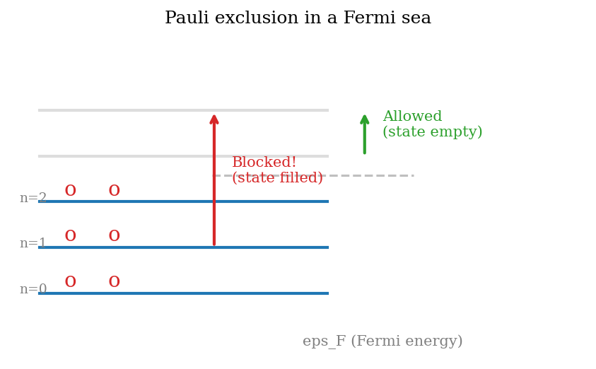
Figure 15: Pauli exclusion prevents scattering into filled states. Excitations can only occur near the Fermi surface, suppressing both collisional thermalisation and heat capacity.

Pauli blocking and cooling efficiency

As the fermion gas reaches degeneracy (\(T \lesssim T_{\rm F}\)), Pauli blocking suppresses not just s-wave scattering but also the final states available for any elastic collision. An elastic collision takes two fermions from states \(\mathbf{k}_1\) and \(\mathbf{k}_2\) and scatters them to \(\mathbf{k}_3\) and \(\mathbf{k}_4\). For this to occur, states \(\mathbf{k}_3\) and \(\mathbf{k}_4\) must be unoccupied. At \(T \ll T_{\rm F}\), the Fermi sea is almost completely filled, and the probability that both final states are empty is suppressed by factors of \(\sim (k_{\rm B}T/\varepsilon_{\rm F})^2\). The elastic collision rate — and hence the thermalisation rate needed for evaporative cooling — thus decreases as \(T^2/T_{\rm F}^2\). This makes evaporative cooling increasingly inefficient as the gas approaches degeneracy, ultimately limiting the achievable temperatures.

Feshbach resonances and interaction tuning

Near a Feshbach resonance — a magnetic-field-tunable scattering resonance — the inter-fermion interaction strength can be varied continuously. The mechanism involves a closed-channel bound state: at a specific magnetic field \(B_0\), a bound state of two atoms in a different internal state (the closed channel) becomes exactly resonant with the two-atom scattering continuum in the open channel. Near this resonance, the s-wave scattering length varies as

\[ a(B) = a_{\rm bg}\left[1 - \frac{\Delta}{B - B_0}\right], \]

where \(a_{\rm bg}\) is the background (off-resonance) scattering length and \(\Delta\) is the resonance width. As \(B\to B_0\), \(|a|\to\infty\) — the scattering length diverges. On one side of the resonance (\(a > 0\)), fermions have an effective repulsive interaction and can form tightly bound molecular bosons that Bose-condense — the BEC side. On the other side (\(a < 0\)), the interaction is attractive and fermions pair near the Fermi surface in the Cooper mechanism of BCS superconductivity — the BCS side. At the resonance itself (the unitary limit, \(|a| = \infty\)), the gas is scale-invariant: the scattering length diverges and drops out, so all thermodynamic quantities are determined solely by the density \(n\) and temperature \(T\).

This BEC–BCS crossover smoothly connects molecular Bose condensation to Cooper pairing without any phase transition. It has been mapped out experimentally in \(^6\)Li and \(^{40}\)K, providing a clean model system for understanding strongly correlated fermions relevant to high-temperature superconductors and neutron stars.

The crossover is characterised by the dimensionless parameter \(1/(k_{\rm F}a)\), where \(k_{\rm F} = (3\pi^2 n)^{1/3}\) is the Fermi wavevector. In the BEC limit (\(1/(k_{\rm F}a) \to +\infty\)), molecules of size \(\sim a\) form and Bose-condense. In the BCS limit (\(1/(k_{\rm F}a) \to -\infty\)), large, overlapping Cooper pairs form at the Fermi surface. At the unitary point (\(1/(k_{\rm F}a) = 0\)), the pair size is comparable to the inter-particle spacing and the system is maximally strongly correlated. The entire crossover is a single superfluid phase — there is no phase transition at \(T = 0\) between the BEC and BCS limits — because both are states with spontaneously broken U(1) symmetry. The crossover can be traversed continuously by sweeping the magnetic field through the Feshbach resonance.

Equation of state measurements via LDA

For a Fermi gas in a harmonic trap with potential \(U(\mathbf{r}) = \frac{1}{2}m(\omega_x^2 x^2 + \omega_y^2 y^2 + \omega_z^2 z^2)\), the local density approximation (LDA) provides a bridge between the trapped (inhomogeneous) system and the uniform (homogeneous) system. The LDA assumes that the gas is locally in equilibrium, with a local chemical potential \(\mu_{\rm local}(\mathbf{r}) = \mu - U(\mathbf{r})\), where \(\mu\) is the global chemical potential fixed by the total atom number. The local density \(n(\mathbf{r})\) is whatever homogeneous density corresponds to \(\mu_{\rm local}(\mathbf{r})\) at temperature \(T\).

Combining TOF imaging (which gives the column-integrated density as a function of position) with the LDA, one can reconstruct the equation of state \(n(\mu, T)\) — or equivalently \(P(\mu, T)\) — of the homogeneous system directly from the density profile of the trapped gas. This technique has been used to measure the equation of state of strongly interacting (unitary) fermions to high precision and to compare with theoretical predictions from quantum Monte Carlo calculations. At the unitary point, the equation of state takes the universal form \(P(\mu, T) = P_{\rm ideal}(\mu, T)\cdot\xi(\mu/k_{\rm B}T)\), where \(\xi\) is a universal function that encodes all the interaction effects. The Bertsch parameter \(\xi(0) \approx 0.376\) (the ratio of the ground-state energy of unitary fermions to that of the ideal Fermi gas) has been measured to a few percent precision in cold-atom experiments.

The power of the cold-atom approach is that it provides clean, controllable model systems for strongly correlated quantum matter. In contrast to electrons in a solid, where disorder, phonons, and fixed lattice structures complicate the comparison with theory, ultracold atoms in optical traps can be prepared with known densities, temperatures, and interaction strengths, and measured with single-atom precision. The equation of state data from unitary fermions has guided the development of improved theoretical techniques (diagrammatic Monte Carlo, functional renormalisation group) that are now being applied to high-temperature superconductors and dense nuclear matter. In this sense, cold-atom physics has become a quantum simulator — a precisely controlled quantum system that encodes the answer to hard many-body problems that cannot be solved analytically.

---

Chapter 15: Weakly Interacting Gases

Mean-field theory and the van der Waals equation

The ideal gas approximation ignores all interactions between particles. A first step beyond it is mean-field theory, in which each particle feels an average field due to all the others. For a real gas with both a short-range hard-core repulsion (modelled as an excluded volume \(b\) per particle) and a longer-range attractive tail (modelled as a mean-field reduction in pressure \(-a(N/V)^2\)), the van der Waals equation of state is

\[ \left(p + a\frac{N^2}{V^2}\right)(V - Nb) = Nk_{\rm B}T. \]

The term \(a(N/V)^2\) represents the mean-field attraction: each molecule experiences a reduction in pressure (inward pull) proportional to the number density squared (since the number of attracting neighbours is proportional to \(N/V\) and the number of molecules at the wall is also \(\propto N/V\)). The term \(Nb\) represents the excluded volume — the volume unavailable because other molecules are already occupying it.

The van der Waals equation is a mean-field result in the sense that it treats all molecular interactions through a single parameter (\(a\)) that represents the average effect of all other molecules, ignoring fluctuations and correlations. Despite its simplicity, it captures the essential physics of the liquid-gas phase transition. Solving for the critical point (where \(\partial p/\partial V = \partial^2 p/\partial V^2 = 0\)):

\[ T_c = \frac{8a}{27bk_{\rm B}}, \qquad V_c = 3Nb, \qquad p_c = \frac{a}{27b^2}. \]

The reduced equation of state \(p/p_c = f(T/T_c, V/V_c)\) is the same for all van der Waals gases — a statement of corresponding states: all gases, when expressed in units of their critical parameters, obey the same equation of state. This is an early example of universality.

The virial (cluster) expansion

For a classical gas with weak interactions, one derives a systematic correction to the ideal gas law by expanding the equation of state in powers of the density. The result is the virial expansion:

\[ \frac{pV}{Nk_{\rm B}T} = 1 + B_2(T)\frac{N}{V} + B_3(T)\left(\frac{N}{V}\right)^2 + \cdots, \]

where \(B_2, B_3, \ldots\) are the virial coefficients. The second virial coefficient is

\[ B_2(T) = -\frac{1}{2}\int d^3r\,f(r), \qquad f(r) = e^{-\beta u(r)} - 1, \]

where \(u(r)\) is the pair interaction potential and \(f(r)\) is the Mayer \(f\)-function. The Mayer function satisfies \(f\to -1\) for \(r < r_{\rm hs}\) (hard-core: the pair cannot overlap) and \(f\to e^{-\beta u} - 1 \approx -\beta u\) for the weak attractive tail.

Hard-sphere gas. For a hard sphere of radius \(r_{\rm hs}\), \(u = \infty\) for \(r < 2r_{\rm hs}\) (twice the radius is the distance of closest approach) and \(u = 0\) otherwise:

\[ B_2^{\rm hs} = -\frac{1}{2}\int_{r<2r_{\rm hs}} (-1)\,d^3r = \frac{1}{2}\cdot\frac{4\pi(2r_{\rm hs})^3}{3} = \frac{4\pi(2r_{\rm hs})^3}{6} = \frac{4}{3}\pi r_{\rm hs}^3\cdot 4 = 4v_{\rm sphere} > 0. \]

More precisely, \(B_2^{\rm hs} = \frac{2\pi}{3}(2r_{\rm hs})^3 = b/4\), where \(b = \frac{2\pi}{3}(2r_{\rm hs})^3\) is the excluded volume parameter in the van der Waals equation (after identification). The positive sign reflects repulsion — the gas pressure is higher than ideal because molecules cannot overlap.

Van der Waals gas. For a gas with a hard core plus a long-range attraction \(u_{\rm att}(r)\):

\[ B_2(T) = b - \frac{a}{k_{\rm B}T}, \]

where \(a = -\frac{1}{2}\int_{r>r_{\rm hs}} u_{\rm att}(r)\,d^3r > 0\) (the attractive part contributes negatively to \(B_2\)). At high temperature \(B_2 \approx b > 0\) (hard-core repulsion dominates); at low temperature \(B_2 \approx -a/k_{\rm B}T < 0\) (attraction dominates). The temperature where \(B_2 = 0\) is the Boyle temperature \(T_{\rm Boyle} = a/(bk_{\rm B})\), where the repulsive and attractive effects cancel and the gas behaves ideally to second order in density.

The virial expansion has a natural convergence radius: it converges whenever the gas is dilute enough that multi-body clusters are rare. The expansion breaks down near the gas-liquid phase transition — a perturbation expansion in density cannot describe the abrupt density discontinuity at a first-order transition. This limitation is related to the Lee–Yang theorem: the grand partition function \(\mathcal{Z}(z)\) as a function of the fugacity \(z = e^{\beta\mu}\) has zeros only on the negative real axis for a real gas at finite volume. In the thermodynamic limit, these zeros can accumulate on the positive real axis, producing the singularity corresponding to the phase transition. When the fugacity is below the Lee–Yang zero closest to the positive real axis, the virial expansion converges; at and above that zero, the expansion fails.

Mayer diagrammatics

The graphical organisation of the virial expansion assigns a cluster diagram to each term. A diagram with \(m\) vertices (molecules) connected by lines (Mayer \(f\)-functions) contributes to the \(m\)-th cluster integral. Connected diagrams contribute to extensive thermodynamic quantities like the free energy; disconnected diagrams cancel in the ratio \(\ln\mathcal{Z}\). The diagrammatic rules are:

• Monomer (single dot): contributes \(1\) — the ideal gas.
• Dimer (two dots connected by a line): contributes \(B_2\) — the two-body correction.
• Triangle (three mutually connected dots): contributes to \(B_3\) — three bodies simultaneously interacting.
• Chain of three (three dots with two lines, not all connected): also contributes to \(B_3\).

The beauty of the diagrammatic expansion is that it systematically organises an exponentially complex many-body problem into a power series, where each term has a clear physical interpretation as a cluster of simultaneously interacting particles.

Quantum virial coefficients

For a weakly quantum gas (small but nonzero \(n\lambda_{\rm dB}^3\)), quantum exchange effects introduce corrections to the virial coefficients even in the absence of interactions. The leading quantum correction to the second virial coefficient is

\[ B_2^{\rm quantum} = \mp\frac{\lambda_{\rm dB}^3}{4\sqrt{2}}, \]

where the minus sign is for bosons and the plus sign is for fermions. For bosons, \(B_2^{\rm quantum} < 0\), meaning the quantum gas has a lower pressure than the classical ideal gas — bosons effectively attract each other statistically. For fermions, \(B_2^{\rm quantum} > 0\), meaning the quantum gas has a higher pressure — fermions effectively repel each other statistically. These quantum corrections become significant when \(n\lambda_{\rm dB}^3 \gtrsim 1\) and diverge as the systems approaches quantum degeneracy, signalling the breakdown of the virial expansion and the need for the full Bose–Einstein or Fermi–Dirac statistics.

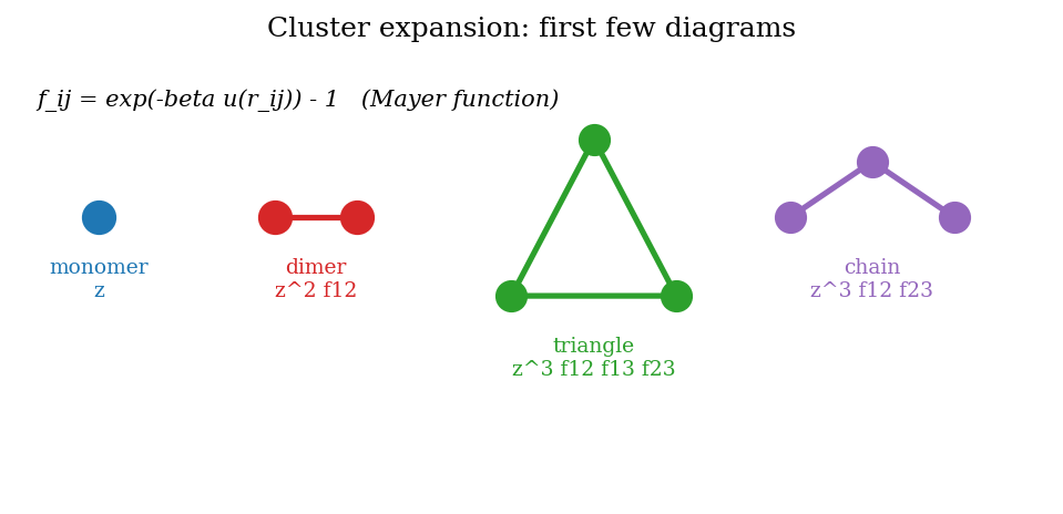
Figure 16: The first few cluster diagrams in the Mayer–Ursell expansion. Each line represents a factor of the Mayer function \(f_{ij} = e^{-\beta u_{ij}}-1\). The second virial coefficient \(B_2\) comes from the dimer diagram; higher virial coefficients involve higher-order connected clusters.

---

Chapter 16: The Ising Model

Introducing interacting spins

Throughout Part I and most of Part II we have dealt with non-interacting systems, where the many-body problem reduces to a one-body problem. Real systems interact, and interactions introduce qualitatively new phenomena: phase transitions, spontaneous symmetry breaking, and universality near critical points. The Ising model is the simplest model to exhibit all of these phenomena.

The Ising model consists of \(N\) spins \(s_i \in \{+1, -1\}\) arranged on a lattice, with an interaction energy between nearest-neighbour pairs and a coupling to an external field:

\[ H = -J\sum_{\langle ij\rangle} s_i s_j - B\sum_i s_i. \]

The coupling constant \(J > 0\) favours alignment (ferromagnetism): antiparallel pairs cost energy \(+J\) while parallel pairs gain \(-J\). This model was proposed by Lenz (1920) and solved in 1D by his student Ernst Ising (1925), who incorrectly concluded — based on the one-dimensional case, which has no phase transition — that ferromagnetism could not arise from this model. Lars Onsager’s exact solution of the two-dimensional Ising model in 1944 showed that the model does have a phase transition in 2D.

The exact 1D solution via transfer matrices

The one-dimensional Ising model on a ring of \(N\) sites (periodic boundary conditions) can be solved exactly using the transfer matrix method. The key idea is to organise the partition function as a matrix product. Write the partition function as a product of local Boltzmann factors:

\[ Z = \sum_{\{s_i\}}\prod_{i=1}^N e^{\beta J s_i s_{i+1} + \beta B(s_i+s_{i+1})/2}. \]

Each factor depends only on the pair \((s_i, s_{i+1})\). Define the \(2\times 2\) transfer matrix \(T\) with elements

\[ T_{s,s'} = e^{\beta(Jss' + B(s+s')/2)}. \]

Explicitly, \(T_{+,+} = e^{\beta(J+B)}\), \(T_{-,-} = e^{\beta(J-B)}\), and \(T_{+,-} = T_{-,+} = e^{-\beta J}\). Summing over all intermediate spins is precisely the operation of matrix multiplication: \(\sum_{s_2} T_{s_1,s_2}T_{s_2,s_3} = (T^2)_{s_1,s_3}\). After summing over all \(N\) spins with periodic boundary conditions (\(s_{N+1} = s_1\)):

\[ Z = \text{Tr}(T^N) = \lambda_+^N + \lambda_-^N, \]

where \(\lambda_\pm\) are the two eigenvalues of the \(2\times 2\) matrix \(T\). Diagonalising \(T\):

\[ \lambda_\pm = e^{\beta J}\cosh(\beta B) \pm \sqrt{e^{2\beta J}\sinh^2(\beta B) + e^{-2\beta J}}. \]

In the thermodynamic limit \(N\to\infty\), the larger eigenvalue dominates: \(Z \approx \lambda_+^N\). The free energy per spin is \(f = -k_{\rm B}T\ln\lambda_+\), and all other thermodynamic quantities follow by differentiation.

The transfer matrix method is not merely a calculational trick. It reveals that the partition function of a one-dimensional model is equivalent to the eigenvalue problem of a matrix — a finite-dimensional linear algebra problem that is always solvable in principle. The method generalises to two dimensions: the 2D Ising partition function can be written as \(\text{Tr}(\mathcal{T}^N)\) where \(\mathcal{T}\) is a \(2^L \times 2^L\) matrix for a lattice of width \(L\), and Onsager’s 1944 solution diagonalises this matrix by mapping it to a free-fermion problem via the Jordan–Wigner transformation.

For \(B = 0\), the eigenvalues simplify dramatically: \(\lambda_+ = e^{\beta J} + e^{-\beta J} = 2\cosh(\beta J)\) and \(\lambda_- = 2\sinh(\beta J)\). The free energy per spin is \(f = -k_{\rm B}T\ln(2\cosh(\beta J))\), and the magnetisation is

\[ m = -\frac{\partial f}{\partial B}\bigg|_{B=0} = 0 \quad \text{for all } T > 0. \]

The 1D Ising model has zero magnetisation at all positive temperatures: there is no phase transition in one dimension. The physical reason is that a single domain wall (a single pair of antiparallel neighbours) costs energy \(2J\) but gains entropy \(k_{\rm B}\ln N\) (it can be placed anywhere along the chain). For any \(T > 0\) and large enough \(N\), the entropy gain outweighs the energy cost and domain walls proliferate, destroying long-range order. In 2D and higher dimensions, domain walls cost energy proportional to their area (not just a single point) and long-range order can survive. The Mermin–Wagner theorem generalises this: in systems with a continuous symmetry (like XY or Heisenberg spins), thermal fluctuations destroy long-range order in 1D and 2D, but not in 3D. For systems with discrete symmetry like the Ising model, the lower critical dimension is 1: order survives at any dimension above 1.

Mean-field theory for the Ising model

Solving the Ising model exactly in 3D remains an open problem. The simplest approximation is mean-field theory: replace the interaction of spin \(i\) with its neighbours by an interaction with the average spin \(m = \langle s\rangle\):

\[ H_{\rm MF} = -\sum_i s_i\,(Jzm + B), \]

where \(z\) is the coordination number (number of nearest neighbours). This decouples into \(N\) independent spins in an effective field \(B_{\rm eff} = Jzm + B\). The self-consistency condition for the mean spin is then

\[ m = \tanh\!\left(\beta(Jzm + B)\right). \]

This transcendental equation can be solved graphically: plot both sides as functions of \(m\) and find the intersections. For \(B = 0\), the trivial solution \(m = 0\) always exists. When \(\beta Jz > 1\), i.e.\ \(T < T_c = Jz/k_{\rm B}\), two additional non-trivial solutions appear at \(m = \pm m_0 \neq 0\), signalling spontaneous magnetisation.

Mean-field critical behaviour

Near \(T_c\) from below, \(m\) is small and we can expand the self-consistency equation. With \(B = 0\) and using \(\tanh x \approx x - x^3/3 + \ldots\):

\[ m = \beta Jz\, m - \frac{(\beta Jz\, m)^3}{3} + \ldots \]

At \(T = T_c\), \(\beta_c Jz = 1\). Writing \(T = T_c - \delta T\) for small \(\delta T > 0\), so \(\beta Jz = T_c/(T_c - \delta T) \approx 1 + \delta T/T_c\):

\[ m\left[1 - (1 + \delta T/T_c)\right] = -\frac{m^3}{3} + \ldots \quad \Rightarrow \quad m^2 \approx \frac{3\delta T}{T_c}. \]

Therefore \(m \propto (T_c - T)^{1/2}\) below \(T_c\). The mean-field critical exponent \(\beta = 1/2\) (not to be confused with inverse temperature) governs the onset of magnetisation.

The susceptibility \(\chi = \partial M/\partial B|_{B=0}\) can be found by differentiating the self-consistency equation with respect to \(B\). Above \(T_c\) where \(m = 0\):

\[ \chi = \frac{\partial m}{\partial B}\bigg|_{m=0} = \beta(1 + Jz\chi) \quad \Rightarrow \quad \chi = \frac{1/k_{\rm B}}{T - T_c}, \]

which is the Curie–Weiss law: the susceptibility diverges as \(T\to T_c^+\) from above, signalling the approach to the ferromagnetic instability.

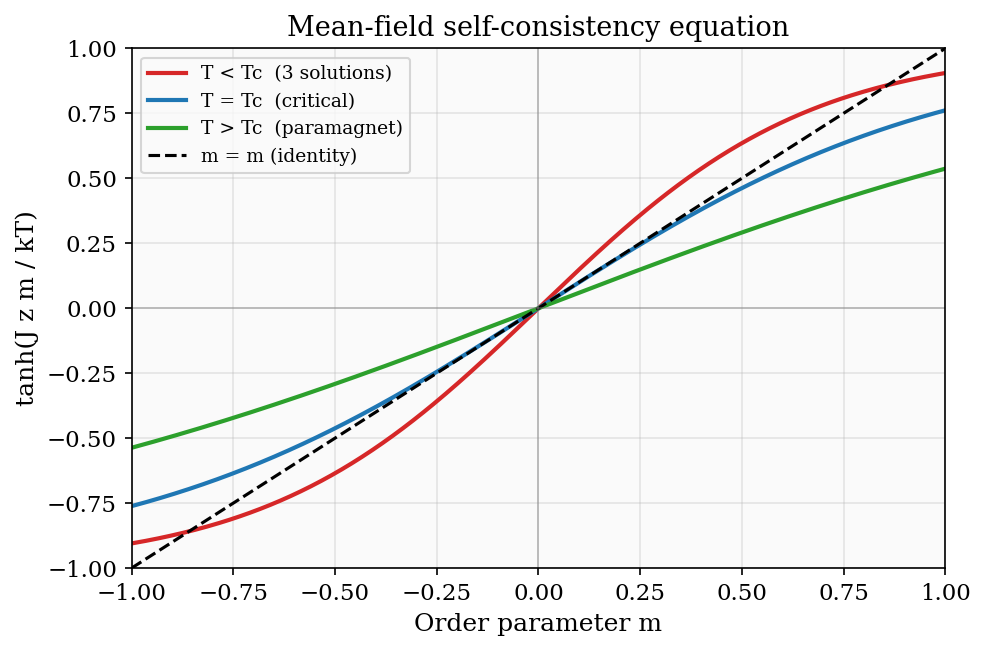
Figure 18: The mean-field self-consistency equation at three temperatures. Below \(T_c\) (red), three solutions exist: the trivially unstable \(m=0\) and two stable magnetised states \(\pm m_0\). At \(T_c\) (blue), the curves are tangent at the origin. Above \(T_c\) (green), only \(m=0\) is stable.

Onsager’s exact solution and universality

Lars Onsager solved the 2D Ising model exactly in 1944, using transfer matrices and the theory of Lie algebras. The key insight is that the transfer matrix for the 2D model can be written in terms of operators that satisfy the algebra of free fermions (via the Jordan–Wigner transformation). The 2D Ising partition function thus reduces to a free-fermion problem, which can be diagonalised exactly. The result is one of the great achievements of 20th-century theoretical physics:

\[ M(T) = \left[1 - \sinh^{-4}\!\left(\frac{2J}{k_{\rm B}T}\right)\right]^{1/8}, \]

with the critical temperature \(k_{\rm B}T_c = 2J/\ln(1+\sqrt{2}) \approx 2.269\,J\). The critical exponent \(\beta = 1/8\) differs dramatically from the mean-field value \(1/2\).

The 2D Ising universality class includes all systems with a one-component order parameter and \(\mathbb{Z}_2\) symmetry in 2D. Critical exponents are compared in the table below:

Exponent	Governs	Mean-field	2D Ising exact
\(\alpha\)	Heat capacity: (C\sim	t	^{-\alpha})
\(\beta\)	Order parameter: \(m\sim(-t)^\beta\)	1/2	1/8
\(\gamma\)	Susceptibility: (\chi\sim	t	^{-\gamma})
\(\nu\)	Correlation length: (\xi\sim	t	^{-\nu})
\(\eta\)	Correlation function at \(T_c\)	0	1/4

where \(t = (T-T_c)/T_c\) is the reduced temperature. The dramatic difference between mean-field and 2D Ising exponents reflects the importance of fluctuations in two dimensions.

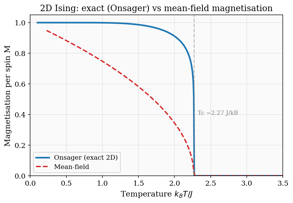
Figure 19: Magnetisation vs temperature for the 2D Ising model. The Onsager exact result (blue, \(\beta = 1/8\)) has a much sharper onset at \(T_c\) than the mean-field prediction (red, \(\beta = 1/2\)). The exact \(T_c^{2D} \approx 2.27\,J/k_{\rm B}\) lies below the mean-field \(T_c = 4J/k_{\rm B}\).

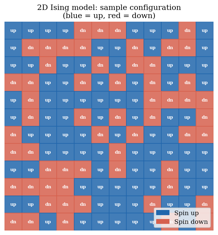
Figure 17: A sample configuration of the 2D Ising model on a \(12\times 12\) lattice. Blue sites have \(s=+1\) and red have \(s=-1\); the majority of spins are up in this realisation, reflecting a net positive magnetisation.

---

Chapter 17: Simulating the Ising Model

The need for numerical methods

The Ising model in 3D — and in 2D away from the critical temperature — resists analytic solution. The configurational space is enormous: for \(N = 100\) spins there are \(2^{100} \approx 10^{30}\) possible states. Direct enumeration is hopeless. Instead, we use Monte Carlo methods to sample the Boltzmann distribution statistically.

Markov chains and the Metropolis algorithm

A Markov chain is a sequence of states \(s^{(1)}, s^{(2)}, \ldots\) where the transition from state \(s^{(t)}\) to \(s^{(t+1)}\) depends only on \(s^{(t)}\) and not on any earlier history. This Markov property — no memory of the past beyond the current state — is what makes the algorithm computationally tractable: we do not need to store the full history of the simulation. For sampling the Boltzmann distribution, we want the chain to converge to the correct stationary distribution \(P_{\rm eq}(s) \propto e^{-\beta H(s)}\). Two properties guarantee convergence: ergodicity (the chain can reach any state from any other in a finite number of steps) and detailed balance. Ergodicity ensures we do not get stuck in a subspace of configurations; detailed balance ensures the stationary distribution is the Boltzmann distribution. For the Ising model with single-spin-flip moves, ergodicity is obvious (any configuration can be reached by flipping spins one at a time), and detailed balance is satisfied by the Metropolis rule.

For sampling the Boltzmann distribution, we want the chain to converge to \(P_{\rm eq}(s) \propto e^{-\beta H(s)}\). A sufficient condition is detailed balance:

\[ P_{\rm eq}(s)\,W(s\to s') = P_{\rm eq}(s')\,W(s'\to s), \]

where \(W(s\to s')\) is the transition probability. The Metropolis algorithm (Metropolis et al., 1953) satisfies detailed balance with the following steps:

1. Choose a spin \(i\) at random.
2. Compute the energy change if spin \(i\) were flipped: \(\Delta E = 2Js_i\sum_{\langle j\rangle} s_j + 2Bs_i\), where the sum is over the nearest neighbours \(j\) of spin \(i\). (Flipping \(s_i \to -s_i\) changes all interaction terms involving \(s_i\).)
3. Accept the flip with probability \(\min(1, e^{-\beta\Delta E})\): always accept moves that lower the energy (\(\Delta E < 0\)); accept moves that raise the energy with a Boltzmann probability.

After many sweeps (\(\sim 10^3 N\) to \(\sim 10^6 N\) depending on proximity to \(T_c\)), the chain has converged and subsequent configurations are distributed according to the Boltzmann distribution. Thermal averages are estimated by averaging observables over configurations.

Critical slowing down

Near the critical temperature, the Metropolis algorithm suffers from critical slowing down. The autocorrelation time \(\tau\) measures how many Monte Carlo steps are needed before two configurations are statistically independent. Near \(T_c\), the correlation length \(\xi\) diverges as \(\xi \propto |T-T_c|^{-\nu}\), and fluctuations on all length scales up to \(\xi\) are correlated. The autocorrelation time grows as

\[ \tau \sim \xi^z \propto |T-T_c|^{-\nu z}, \]

where \(z\) is the dynamical critical exponent. For the Metropolis algorithm (single-spin-flip dynamics, corresponding to Model A in the Hohenberg-Halperin classification), \(z \approx 2\) for the 2D Ising model. Since \(\nu = 1\) for the 2D Ising model, \(\tau \sim |T - T_c|^{-2}\), which diverges rapidly as \(T\to T_c\). Obtaining statistically independent samples becomes exponentially expensive near the critical point.

Cluster algorithms overcome critical slowing down by proposing collective moves that flip entire clusters of aligned spins simultaneously. In the Wolff algorithm, a cluster is grown by adding each neighbouring aligned spin with probability \(1 - e^{-2\beta J}\), then the entire cluster is flipped. The Wolff algorithm has a dynamical exponent \(z \approx 0.3\) for the 2D Ising model — dramatically smaller than the single-spin-flip value of 2 — making it far more efficient near \(T_c\).

Block-spin renormalisation group

A powerful conceptual framework for understanding universality near phase transitions is the renormalisation group (RG), developed by Kadanoff and Wilson in the 1960s–70s. The core idea is to reduce the number of degrees of freedom by systematically averaging (coarse-graining) over microscopic details.

In the block-spin version, one divides the lattice into blocks of \(b \times b\) spins and replaces each block by a single effective spin. For the simplest case \(b = 2\) (replacing \(2\times 2\) blocks by a single spin), the partition function of the original system can be written in terms of the block spins, and the resulting system has the same form as the original Ising model — just with a renormalised coupling \(K' = f(K)\), where \(K = \beta J\). The renormalisation group transformation maps \(K \to K'\).

The fixed point \(K^* = f(K^*)\) is special: the system is statistically self-similar at all length scales, which is exactly the property of a system at the critical temperature. The linearised flow near \(K^*\) is characterised by the eigenvalue \(\lambda = df/dK|_{K^*}\). The correlation length exponent is \(\nu = \ln b/\ln\lambda\) (where \(b\) is the rescaling factor). Perturbations that grow under RG (eigenvalue \(|\lambda| > 1\)) are relevant and drive the system away from the critical point; perturbations that shrink (\(|\lambda| < 1\)) are irrelevant and do not affect the critical exponents.

Iterating the block-spin transformation generates a flow in the space of couplings. Fixed points of this flow correspond to universality classes. The critical exponents are determined by the linearised flow near the critical fixed point, explaining why all systems in the same universality class share the same exponents regardless of microscopic details.

Finite-size scaling

Simulations are necessarily performed on finite lattices of linear size \(L\), and the critical singularities are rounded by finite-size effects: the correlation length cannot exceed \(L\), so the divergence \(\xi\to\infty\) is cut off at \(\xi \sim L\). The finite-size scaling hypothesis states that near \(T_c\), all observables depend on temperature and system size through the dimensionless combination \((T - T_c)L^{1/\nu}\):

\[ \chi(T, L) = L^{\gamma/\nu}\,\tilde{\chi}\!\left[(T-T_c)L^{1/\nu}\right], \]

where \(\tilde{\chi}\) is a universal scaling function. By measuring the susceptibility (or other observables) on lattices of different sizes \(L\) and plotting \(\chi L^{-\gamma/\nu}\) vs \((T-T_c)L^{1/\nu}\), all the curves should collapse onto a single universal function — a technique called data collapse. The value of \(\nu\) (and other exponents) that produces the best collapse can be extracted from the data, providing a precision measurement of the critical exponents without any analytic computation.

Finite-size scaling also allows a reliable determination of \(T_c\) from simulation data. At the exact critical temperature, the scaled susceptibility \(\chi L^{-\gamma/\nu}\) is independent of \(L\) (all curves cross at the same point), since \(\tilde{\chi}(0)\) is a universal constant. The crossing point of susceptibility curves for different system sizes \(L\) is therefore an estimator of \(T_c\) that converges rapidly with increasing \(L\). This approach, combined with the data collapse technique, has been used to determine the critical temperature and exponents of the 3D Ising model (\(T_c \approx 4.51 J/k_{\rm B}\), \(\beta \approx 0.326\), \(\nu \approx 0.630\), \(\gamma \approx 1.237\)) to five or more significant figures. The 3D Ising universality class governs the liquid-gas critical point of real fluids (including water and carbon dioxide), the ferromagnetic transition in uniaxial magnets, and polymer collapse transitions — all sharing the same set of critical exponents to high precision, confirming the universality hypothesis first stated by Kadanoff and proven by Wilson’s renormalisation group.

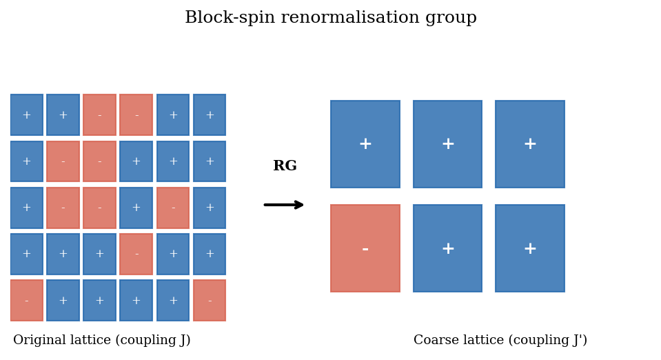
Figure 20: Block-spin renormalisation: the original fine lattice (left) with coupling \(J\) is coarse-grained to a lattice with half the linear density (right) and a renormalised coupling \(J'\). Repeating this procedure generates a flow in coupling-constant space.

---

Chapter 18: Statistical Mechanics Beyond Physics

Transferability of the framework

Statistical mechanics began as a tool for understanding gases and solids, but its conceptual apparatus — microstates, entropy, the Boltzmann distribution, partition functions, phase transitions — applies to any system with a large number of interacting degrees of freedom and some form of disorder or randomness. The closing lectures of PHYS 359 survey a few of the fields that have borrowed heavily from stat mech.

Maximum entropy inference

Before turning to specific applications, note that the Boltzmann distribution can be derived by a purely information-theoretic argument due to Jaynes (1957). Given a probability distribution \(\{p_s\}\) over microstates, the Shannon entropy is \(H = -\sum_s p_s \ln p_s\). If the only constraints are \(\sum_s p_s = 1\) (normalisation) and \(\sum_s p_s E_s = \bar{E}\) (fixed average energy), the distribution that maximises \(H\) subject to these constraints is found by introducing Lagrange multipliers \(\lambda_0\) and \(\beta\) for the two constraints:

\[ \frac{\partial}{\partial p_s}\left[-\sum_s p_s\ln p_s - \lambda_0\sum_s p_s - \beta\sum_s p_s E_s\right] = 0 \quad \Rightarrow \quad -\ln p_s - 1 - \lambda_0 - \beta E_s = 0. \]

Solving: \(p_s = e^{-1-\lambda_0}e^{-\beta E_s}\). Normalisation fixes \(e^{1+\lambda_0} = \sum_s e^{-\beta E_s} = Z(\beta)\), so

\[ p_s = \frac{e^{-\beta E_s}}{Z(\beta)}. \]

This is exactly the Boltzmann distribution. The parameter \(\beta\) is the Lagrange multiplier for the energy constraint — it is determined by the condition \(\sum_s p_s E_s = \bar{E}\), which is simply the requirement that the average energy matches the given value. The partition function \(Z(\beta) = \sum_s e^{-\beta E_s}\) is the Laplace transform of the density of states \(g(E)\): \(Z(\beta) = \int g(E)e^{-\beta E}\,dE\).

This maximum entropy principle (MaxEnt) has proven useful far beyond thermodynamics. In data analysis, reconstruction problems, and machine learning, the MaxEnt distribution is the least-biased distribution consistent with the given constraints — it assumes nothing beyond what the data tell us. The Ising model itself can be derived as the MaxEnt distribution for binary data with pairwise correlations specified.

Spin glasses, networks, and neural systems

The Hopfield model of neural networks (Hopfield, 1982) maps memory storage onto the energy landscape of an Ising-like system. Neurons are modelled as binary units (\(s_i = \pm 1\)), and the synaptic weights are chosen according to the Hebb rule:

\[ J_{ij} = \frac{1}{N}\sum_{\mu=1}^p \xi_i^\mu \xi_j^\mu, \]

where \(\boldsymbol{\xi}^\mu = (\xi_1^\mu, \ldots, \xi_N^\mu)\) with \(\xi_i^\mu = \pm 1\) are the \(p\) stored patterns. This choice of weights ensures that each stored pattern is a local energy minimum of the Ising Hamiltonian \(H = -\sum_{ij} J_{ij} s_i s_j\). The dynamics of memory retrieval — where a noisy input pattern evolves toward the stored memory — is Glauber dynamics (equivalent to the Metropolis algorithm) for this Hamiltonian. The overlap \(m^\mu = (1/N)\sum_i s_i \xi_i^\mu\) measures how similar the current state is to pattern \(\mu\) and serves as the order parameter: \(m^\mu \approx 1\) means pattern \(\mu\) has been recalled.

The capacity of the Hopfield network — how many patterns \(p\) can be stored and reliably recalled — is \(p_{\rm max} \approx 0.138N\). Above this threshold, spurious minima proliferate and recall fails. This capacity calculation uses the replica method from spin glass theory, illustrating the deep connection between neural computation and the statistical mechanics of disordered systems.

The Boltzmann machine

A Boltzmann machine is a generative model consisting of visible units (representing observable data) and hidden units (representing latent variables), with Ising-like couplings between all pairs. The model defines a probability distribution over configurations via \(P(\mathbf{s}) \propto e^{-\beta H(\mathbf{s})}\). Training the model on data means adjusting the couplings \(J_{ij}\) to minimise the KL divergence between the data distribution and the model distribution. The gradient of the log-likelihood with respect to \(J_{ij}\) is

\[ \frac{\partial \ln P}{\partial J_{ij}} = \langle s_i s_j\rangle_{\rm data} - \langle s_i s_j\rangle_{\rm model}, \]

the difference between the correlations under the data distribution and the model distribution. This is analogous to the energy difference in the Metropolis accept/reject step: the model is nudged toward configurations that agree with the data. Computing \(\langle s_i s_j\rangle_{\rm model}\) requires sampling from the Boltzmann distribution — a Monte Carlo calculation — which is computationally expensive for large systems. Restricted Boltzmann machines (RBMs), where hidden and visible units only connect to each other (no within-layer connections), allow efficient computation using the contrastive divergence approximation, making them practical for machine learning applications.

Evolutionary biology and game theory

The fitness landscape of evolutionary biology — a high-dimensional surface where each point is a genome and the height is reproductive fitness — is the biological analogue of an energy landscape. Evolutionary dynamics under mutation and selection resembles a random walk on this landscape. The quasispecies equation of Eigen and Schuster describes the evolution of a population of sequences with mutation rate \(\mu\) and replication fitness \(f_\sigma\) for sequence \(\sigma\):

\[ \frac{d n_\sigma}{dt} = \sum_{\sigma'} Q_{\sigma\sigma'} f_{\sigma'} n_{\sigma'} - \phi(t) n_\sigma, \]

where \(Q_{\sigma\sigma'}\) is the mutation matrix (probability that sequence \(\sigma'\) gives rise to \(\sigma'\) upon replication) and \(\phi\) maintains normalisation. When the mutation rate \(\mu\) exceeds a critical value — the error threshold — information cannot be maintained and the population delocalises across genome space. This error catastrophe is formally analogous to the paramagnetic disordering transition in the Ising model: the “temperature” of the evolutionary system is the mutation rate, and the “order parameter” is the concentration of the master sequence. RNA viruses operate near but below the error threshold — high mutation rates allow rapid adaptation to changing environments, but crossing the threshold would destroy genetic information entirely.

Information theory and the partition function

The connection between statistical mechanics and information theory runs deeper than the analogy between Boltzmann entropy and Shannon entropy. Consider a long message consisting of symbols drawn from an alphabet. The Shannon entropy per symbol, \(H = -\sum_i p_i\log_2 p_i\), gives the minimum number of bits needed to transmit the message losslessly (Shannon’s source coding theorem). But Boltzmann entropy also measures the information content of a macrostate: \(S = k_{\rm B}\ln\Omega\) counts the number of bits (multiplied by \(k_{\rm B}\ln 2\)) needed to specify the microstate given the macrostate. The two entropies are literally the same function, differing only in units and the base of the logarithm.

High-entropy macrostates in statistical mechanics correspond to maximally disordered microstates: the thermodynamic equilibrium state is the one that is hardest to describe, because it contains the most microscopic information. The approach to equilibrium (entropy increase) is therefore the approach to the maximally disordered state — the state about which we know the least, given only the macroscopic constraints. This is yet another perspective on the MaxEnt principle: equilibrium is the state of maximum ignorance consistent with the macroscopic observations.

The free energy \(F = U - TS\) has a compelling information-theoretic interpretation. It measures the amount of energy available to do useful work — energy that is not locked in the randomness of thermal fluctuations. The term \(TS\) is the “thermal trash” — energy that is degraded into heat and cannot be recovered. A system at low entropy (highly ordered microstate) has a high free energy and can do lots of work; a system at high entropy (disordered) has used up its capacity for work. The second law of thermodynamics — that free energy is minimised in equilibrium — is thus the statement that systems spontaneously degrade their ability to do useful work by maximising disorder.

The Laplace transform connection between \(Z(\beta)\) and the density of states \(g(E)\) is particularly elegant. Writing \(Z(\beta) = \int_0^\infty g(E)e^{-\beta E}\,dE\), the partition function is the Laplace transform of the density of states. The inverse Laplace transform recovers \(g(E)\) from \(Z(\beta)\). In Bayesian inference, \(Z(\beta)\) plays the role of the model evidence (or marginal likelihood): the probability of the data given the model, integrated over the parameter \(\beta\). Large \(Z\) means the model is broadly consistent with many configurations weighted by the Boltzmann factor — the model explains the data without overfitting. Small \(Z\) means the model is concentrated on a few configurations inconsistent with the energy constraint — the model is either too constrained or wrong. Bayesian model selection thus formally parallels the selection of the equilibrium ensemble that best describes the macroscopic constraints.

The unity of the framework

The most important lesson of this course is not any individual formula — not the Boltzmann factor, not the Sackur–Tetrode equation, not the Debye \(T^3\) law — but the recognition that a single conceptual framework underlies an astonishing variety of phenomena. The partition function \(Z = \sum_s e^{-\beta E_s}\) is, from the perspective of Bayesian inference, the model evidence — the normalisation factor that converts likelihoods into probabilities. Maximising the logarithm of \(Z\) with respect to model parameters is equivalent to maximising the marginal likelihood, the standard criterion for Bayesian model selection. The free energy \(F = -k_{\rm B}T\ln Z\) appears in machine learning as the negative of the evidence lower bound (ELBO): minimising the ELBO over a variational distribution \(q\) is equivalent to maximising a free energy, and mean-field variational inference is precisely the mean-field theory of statistical mechanics applied to the problem of approximate Bayesian inference. The Hopfield model, the Boltzmann machine, the quasispecies model, and spin glasses all use the same mathematical vocabulary.

The deep reason for this universality is that the MaxEnt principle — the most probable macrostate is the one that maximises entropy subject to constraints — is a statement about probability theory itself, not about physics. Whenever a system has many degrees of freedom, some conserved quantities, and we ask about its typical macroscopic state, the answer is always the maximum-entropy state consistent with the constraints. Physics provided the first domain in which this principle was systematically developed, but the principle belongs to all of science. Once internalised, the partition function, the free energy, and the Boltzmann distribution appear everywhere — in the structure of language models, in the dynamics of ecological communities, in the folding of proteins, and in the behaviour of financial markets. The statistical mechanics developed in this course is, in the broadest sense, the theory of probable things.

The journey from Chapter 1 to Chapter 18 traces an arc from simple combinatorics — counting the microstates of an Einstein solid — through the classical and quantum distributions, to the experimental realisation of quantum phases and the application of statistical mechanics to biology, computation, and social systems. The central unifying object is the partition function, which compresses the entire thermal physics of a system into a single generating function. The central unifying principle is the Boltzmann distribution, which tells us that equilibrium is not the state of lowest energy but the state of lowest free energy — the state that balances energy against entropy. And the central unifying insight is that large numbers of interacting degrees of freedom, far from being intractable, often simplify dramatically: the thermodynamic properties of a mole of gas depend on only a handful of macroscopic parameters, regardless of the detailed interactions among \(10^{23}\) molecules. This simplification — the emergence of macroscopic order and universality from microscopic complexity — is the deepest gift of statistical mechanics to our understanding of nature.

---

End of course notes.