Course Introduction and Motivation

Why This Course? What Is It About?

CS476/676 Computational Finance is a course that teaches basic computational methods for solving interesting and important problems in finance using computers — a domain commonly referred to as FinTech (financial technology). The course sits at the intersection of rigorous mathematics, algorithmic thinking, and real-world financial markets, and it is offered within the Computer Science department for reasons that are both practical and intellectual.

Why Is Computational Finance Offered in CS?

A natural question is why a subject that sounds like it belongs in an economics or finance faculty is housed in Computer Science. The answer has two parts. First, the financial industry has an immense and growing need for CS talent: the algorithms, software systems, and data pipelines that underpin modern banking, trading, and risk management are built and maintained by computer scientists and software engineers. Second, the career data reflects this reality — many CS graduates find themselves working in the financial industry, whether in quantitative trading, risk technology, data science, or software development for financial platforms.

CS Relevance: Voices from Industry

The demand for technically trained computer scientists in finance is not merely an academic observation; it is articulated loudly by senior leaders at the world’s largest financial institutions.

“Everything we do is underpinned by math and a lot of software.” — Goldman Sachs CFO Marty Chavez, speaking to a Harvard audience in January 2017.

This remark captures the essence of modern investment banking: every trade, every risk calculation, every client interaction is mediated by software systems built on mathematical foundations.

“We’re in the technology business. Our product happens to be banking, but largely that’s delivered through technology.” — Nova Scotia Bank CEO Brian Porter, to The Globe and Mail, 2016.

Porter’s framing is striking — he does not describe his institution as a bank that uses technology, but as a technology company whose product is banking. The distinction signals how thoroughly software has become the core delivery mechanism of financial services.

“If I have a choice to choose somebody who has experience in technical or delivery experience or data mining, I would rather pick up that expertise and teach them banking than taking somebody from another bank who is no further ahead than we are.” — Jeff Henderson, Executive VP and Chief Information Officer at TD, to The Financial Post, 2017.

Henderson’s statement is perhaps the most directly relevant to CS students: banks would rather hire a strong computer scientist and train them in finance than hire a finance person with weak technical skills. This is a compelling argument for why a computational finance course belongs in CS.

Beyond individual hiring preferences, banks and financial institutions are making structural investments in technical talent near universities. Examples in the Waterloo region include Borealis (the RBC-funded AI research institute), the CIBC data lab, Manulife, and Sun Life, all of which have established research partnerships or offices near the University of Waterloo. The broader trend is clear: many skilled technical professionals now work in the financial industry, and this flow will only accelerate.

Background Assumed

The course assumes students have a working knowledge of programming (implementation of algorithms in code), calculus and linear algebra (derivatives, integrals, matrix operations), and statistics (probability distributions, expectation, variance, the normal distribution, conditional expectation). Some mathematical maturity is expected — the ability to follow and construct rigorous arguments — but crucially, no prior finance background is assumed. All financial concepts will be introduced from first principles.

Students are encouraged to review the following before proceeding: basic statistics and probability, expectation, conditional expectation, variance, the normal distribution, calculus, and linear algebra.

What Is This Course About? Risk and Its Management

The intellectual heart of the course is the concept of risk — uncertainty in financial markets that critically affects the operations of financial institutions, companies, universities, individuals, and societies at large. Stock and commodity prices do not move smoothly; they exhibit mountains and valleys in zigzag, Brownian-motion-like movements that make future values inherently unpredictable. Risk management — the systematic analysis, measurement, and reduction of financial uncertainty — is a major agenda of both government and financial institutions, and financial markets have a significant impact on society as a whole.

Two fundamental questions motivate the field: Can uncertainty be analyzed and measured? Can risk be reduced, and if so, how? The answer to both is yes, and mathematics and computing play a key role. Specifically, mathematical and computational methods underpin investment strategy analysis, asset valuation, risk management, and data-driven pattern recognition.

Derivative Markets and Their Importance

This course focuses on financial instruments in a derivative market, which is one of the largest financial markets in the world. Derivative instruments have complex, nonlinear risk profiles that make them particularly challenging — and particularly rewarding — to analyze. Importantly, the models and computational methods developed in this course go beyond the derivative markets and apply broadly to quantitative finance.

Financial derivatives are major news, topics of social discussion, and even the subject of popular films such as The Big Short and Margin Call. CBS’s 60 Minutes described derivatives as “too important to ignore and too complex to explain.” Warren Buffett famously called financial derivatives “weapons of mass destruction.” These characterizations underscore why rigorous computational methods for understanding derivatives are so valuable: the stakes are high.

Course Outline: Main Topics

The course covers the following major topics, progressing from financial definitions through mathematical theory and into practical computation.

The first topic is basic financial derivatives: definitions and uses. Students will learn what options, futures, and other derivatives are, and why they are used in practice. The second topic is no-arbitrage pricing theory: a financial theory based on the principle of trading without risk-free profit opportunities. This principle, which will be developed carefully, is the foundation for all rigorous option pricing.

The third major topic is stochastic asset price models, which come in two flavors: discrete time and discrete state models based on the binomial lattice, and continuous-time models based on Brownian motion. These models capture the random movement of asset prices over time.

On the mathematical side, the course introduces stochastic differential equations (SDEs), which describe how asset prices evolve in continuous time under randomness. Students will learn the tools of Ito’s calculus, the branch of mathematics that extends ordinary calculus to functions of stochastic processes. The course also covers partial differential equations (PDEs), which arise naturally from the no-arbitrage pricing arguments, and optimization theory, which underlies portfolio construction and model calibration.

On the computational side, the course covers binomial lattice option valuation, Monte Carlo simulations for estimating expected payoffs, techniques for analyzing dynamic trading strategies, dynamic programming for solving multi-period decision problems, numerical methods for solving PDEs, portfolio optimization, model calibration (fitting model parameters to market data), and data-driven optimization.

---

A Brief History of Options

History of Options

The history of financial options stretches back more than two millennia, long predating the formal mathematical machinery that would eventually be developed to price them. Understanding this history illuminates why options exist and what economic purposes they serve.

Thales of Miletus and the Olive Harvest (332 BC)

The earliest recorded option-like transaction is attributed to Thales of Miletus, an ancient Greek philosopher, astronomer, and mathematician. Around 332 BC, Thales used his knowledge of star positions — a sophisticated observational tool in antiquity — to predict that the coming olive harvest would be exceptionally large. Reasoning from this astronomical forecast, he anticipated that demand for olive presses (the equipment used to extract olive oil) would be very high at harvest time.

To profit from his prediction, Thales paid the owners of olive presses a fee in advance in order to secure the right to use the presses during the harvest period. The contract was agreed at time \(t = 0\), before the harvest, for a price that reflected the present uncertainty about demand. The underlying price in this transaction was the market rental price of an olive press at harvest time \(T\). The diagram of this relationship places Thales on one side, the press owner on the other, with the contract specifying the olive press price \(S\) at harvest time \(T\) linking the two parties.

Thales was the holder of the contract — he paid for the right, and he could choose to exercise it or not. The press owner was the writer — having accepted payment, they had the obligation to make the presses available if Thales chose to use them. When the harvest indeed proved large and rental prices rose, Thales exercised his right, renting the presses at the pre-agreed lower price and subletting them at the prevailing high market price, earning a profit. If the harvest had been poor and rental prices had fallen below his pre-agreed price, Thales would simply have walked away, losing only his initial payment. This is precisely the asymmetric payoff structure that defines a modern financial option.

Tulip Bulb Mania in 17th Century Holland

The next landmark in option history is considerably more dramatic. In the 1600s, tulips became prized possessions in Holland, with rare varieties commanding extraordinary prices. The tulip market attracted participants ranging from professional flower growers and wholesalers to ordinary citizens speculating on price movements, and the resulting price spiral is widely regarded as possibly the first financial bubble in recorded history.

Within this feverish market, growers and wholesalers used complex option contracts to reduce their risk exposure to the tulip bulb price at the harvest time \(T\). The contracts worked in two directions. Tulip bulb growers bought contracts that allowed them to sell at today’s price, protecting them against the risk that the price would fall by harvest time — these were put-like contracts. Tulip wholesalers bought contracts that allowed them to buy at today’s price, protecting them against the risk that the price would rise — these were call-like contracts. In both cases, the underlying asset \(S_t\) was the tulip price. The diagram of this relationship shows the holder on one side and the writer on the other, with the contract specifying the right to buy or sell tulip at harvest time \(T\).

Beyond these hedging uses, ordinary people began using options speculatively, betting on tulip prices continuing to rise. Options provided leverage: a small upfront payment could secure the right to profit from a much larger movement in the underlying price. However, leverage cuts both ways. For a call option, if the underlying price falls below the strike price at expiry, the option’s value is zero — a 100% loss on the premium paid. When the tulip market bubble burst, those who had bought call options lost everything they had invested in them, and the Dutch economy went into recession. The episode stands as a stark early illustration of how derivative instruments amplify both gains and losses.

Derivative Trading: A Risky Business

The aftermath of tulip mania shaped public and regulatory attitudes toward derivative trading for generations. Derivative trading acquired a bad reputation — it was seen as inherently speculative and socially harmful. Because derivative trading was unregulated for a long time and had demonstrated its capacity for economic disruption, option trading was actually made illegal from 1733 to 1860, a ban lasting nearly 130 years. This regulatory episode underscores that derivatives have always attracted controversy: their potential for amplifying risk is real, and the question of how to measure and manage that risk is precisely what this course is about.

Listed Options Markets

The rehabilitation of option trading as a legitimate financial activity happened gradually. In the late 19th century, Russel Sage, an American financier, traded calls and puts over-the-counter — that is, through private bilateral agreements rather than on a formal exchange. Sage was the first to identify empirically that option value is related to the price of the underlying asset and to the prevailing interest rate, foreshadowing the formal theory that would come decades later.

The modern era of listed options markets began in 1973 with the opening of the Chicago Board of Options Exchange (CBOE), the first formal exchange dedicated to standardized option contracts. The existence of a centralized exchange made contracts more transparent, more liquid, and more accessible to a wide range of participants.

Also in 1973, the Black-Scholes option pricing methodology was published, providing for the first time a rigorous mathematical formula for determining the fair value of a European option. This pricing theory helped participants determine fair values and dramatically increased market liquidity by giving buyers and sellers a common, theoretically grounded framework for negotiation.

The Quest for an Option Pricing Formula

The intellectual history of option pricing is a story of gradual convergence on a rigorous solution. We know at expiry \(T\) that \(V_T = \text{payoff}(S_T)\). We know the current price \(S_0\). The question is: what is the fair value \(V_0\) today?

The solution approach is to determine the relationship between the underlying price \(S\) and the option value \(V\) at any time \(t\) — that is, to find the function \(V(S, t)\). Once this function is known, today’s fair value is simply \(V(S_0, 0)\).

The key contributors to this quest, in historical sequence, were as follows. First, Louis Bachelier submitted a seminal doctoral thesis at the University of Paris in 1900, in which he modeled stock prices as a random walk and derived an early call pricing formula — arguably the founding document of mathematical finance. Second, Paul Samuelson (Nobel laureate in economics) rediscovered Bachelier’s thesis around 1950 and refined the model, introducing the lognormal model for asset prices. Third, Ed Thorp derived the correct option pricing formula in 1965, though without providing a formal proof of why it was correct. Finally, the seminal works of Fischer Black, Myron Scholes, and Robert Merton in 1970 provided the complete, rigorous derivation using no-arbitrage arguments and stochastic calculus. Black-Scholes and Merton received the Nobel Prize in Economics in 1997 (Black had died in 1995).

In this course we will focus on stock options with expiry \(T \leq 1\) (at most one year), and we will reasonably ignore randomness in the interest rate. Before discussing option pricing, we need some basic definitions.

A stock is a share in the ownership of a company. A dividend is a payment made to shareholders out of the company’s profits. An important subtlety is that when a stock pays a dividend to its shareholders, the holder of an option on that stock receives nothing — the option holder does not own the stock, only the right to buy or sell it. For this reason, an option is said to be dividend protected: its payoff function is defined purely in terms of the stock price, not the dividend stream.

---

Financial Options — Definitions, Payoffs, and the Pricing Problem

Financial Options: The Basic Definition

A financial option (also called a financial derivative) is a financial contract stipulated today at time \(t = 0\). The defining feature of such a contract is that its value at the future expiry date \(T\) is determined exactly by the market price of an underlying asset at \(T\). The contract is entered into between two parties: the holder, who buys the option and enters a long position, and the writer, who sells the option and enters a short position. This relationship is often depicted with a diagram showing the holder on the left connected to the writer on the right, with the contract — specifying the underlying price process \(S_t\), the expiry \(T\), and the payoff function \(\text{payoff}(S_T)\) — in the middle.

The Underlying Asset

The underlying asset \(S_t\) can be any of a wide variety of financial instruments: a stock (a share in a company), a commodity (such as oil, gold, or agricultural products), a market index (such as the S&P 500), an interest rate or bond, or an exchange rate (the price of one currency in terms of another). In each case, the underlying evolves randomly over time. We let \(S_t\), or equivalently \(S(t)\), denote the underlying price at time \(t\). This quantity is a stochastic process — a mathematical object that assigns a random value to each point in time. Intuitively, a stochastic process is a time-indexed family of random variables; at each time \(t\), \(S_t\) is uncertain until that moment arrives and the market price is observed.

The Insurance Interpretation

Knowing how the contract’s future value relates to the underlying asset allows the option to be used as a form of financial insurance. The holder has bought protection against an adverse movement in the underlying price; the question is how much that protection is worth today. Equivalently, the writer has sold that protection and taken on the corresponding risk (uncertainty); the question is how much compensation the writer should receive today for bearing that risk. The diagram of the cash flow shows a premium \(V_0\) flowing from holder to writer at time \(t = 0\), and a payoff \(V_T = \text{payoff}(S_T)\) flowing from writer to holder at time \(T\).

European Calls and Puts

The two most fundamental types of option are the call and the put, each available in European and American varieties.

A European call option is the right to buy the underlying asset at a pre-specified strike price \(K\). Crucially, this right can only be exercised at the expiry date \(T\) — not before. There is an important asymmetry: the holder has the option to exercise but no obligation to do so, while the writer has the obligation to sell at \(K\) if the holder exercises.

A European put option is the right to sell the underlying asset at the strike price \(K\), again exercisable only at expiry \(T\).

An American put option is the right to sell the underlying asset at the strike price \(K\), with the right exercisable at any time from the present up to and including the expiry \(T\). The ability to exercise early makes American options harder to price than their European counterparts.

We let \(V(S(t), t)\), or \(V_t\), denote the option value at time \(t\).

Payoff Functions

The central question of option pricing is: what is the fair value \(V_0\) of the option today? And relatedly: how should a writer hedge the risk they have taken on? Before addressing pricing, we first determine the payoff functions — the value \(V_T = \text{payoff}(S_T)\) at expiry — for calls and puts.

Call Payoff at Expiry

At expiry \(T\), the holder of a call option compares the market price \(S_T\) against the strike price \(K\). If \(S_T \leq K\), the holder can buy the underlying more cheaply on the open market than by exercising the option, so it is rational not to exercise, and the call expires worthless with \(V_T = 0\). If \(S_T \geq K\), the holder exercises the call, receiving the underlying worth \(S_T\) and paying only \(K\), for a net gain of \(S_T - K\). Therefore:

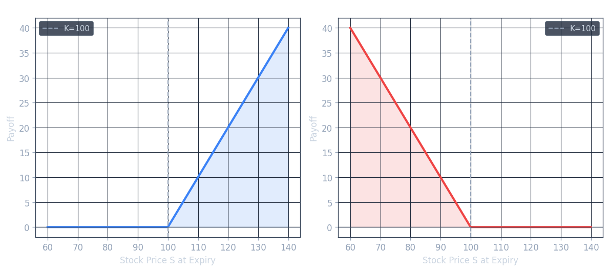
\[ V_T = \text{payoff}(S_T) = \max(S_T - K,\, 0) = \begin{cases} S_T - K & \text{if } S_T \geq K \\ 0 & \text{otherwise} \end{cases} \]

The call payoff diagram is a “hockey stick” shape: it is flat at zero for all \(S_T \leq K\), and then rises linearly with slope 1 for \(S_T > K\), with the kink occurring exactly at the strike price \(K\).

Put Payoff at Expiry

For a put option, the analysis is symmetric. If \(S_T \leq K\), the holder can sell the underlying at the strike price \(K\) — which is above the market price — and gains \(K - S_T\). If \(S_T \geq K\), it is not rational to exercise (the holder could sell at a higher price on the open market), so the put expires worthless. Therefore:

\[ V_T = \text{payoff}(S_T) = \max(K - S_T,\, 0) = \begin{cases} K - S_T & \text{if } S_T \leq K \\ 0 & \text{otherwise} \end{cases} \]

The put payoff diagram is also a hockey stick, but mirrored: it is zero for \(S_T \geq K\) and rises linearly (with slope -1 in \(S_T\) as \(S_T\) falls below \(K\).

Exotic Payoffs: The Straddle

Many other payoff functions have been constructed beyond simple calls and puts. A straddle is a combination of a call and a put with the same strike and expiry:

\[ \text{payoff}(S_T) = \max(S_T - K, 0) + \max(K - S_T, 0) \]

The straddle’s payoff diagram has a V-shape centered at \(K\): it pays \(|S_T - K|\) regardless of which direction the underlying moves. This makes a straddle a bet on volatility rather than on direction — the holder profits if the underlying moves significantly in either direction from \(K\).

Concrete Examples

To make these definitions concrete, consider two tulip-market examples from the historical context. A bulb wholesaler can purchase a call option to have the right to buy tulip bulbs at a fixed price of $0.50 per dozen in three months — this protects the wholesaler against the price rising above $0.50. A bulb grower can purchase a put option to have the right to sell tulip bulbs at a fixed price of $1.00 per dozen in three months — this protects the grower against the price falling below $1.00. A speculative bet on the underlying price can be placed by trading either the underlying itself \(S_t\) or the option value \(V_t\).

The Leverage Effect

It is important to appreciate that an option is more risky relative to the underlying — this is the leverage effect. The relative move in the underlying is typically much smaller than the relative move in the option value:

\[ \left| \frac{S_T - S_0}{S_0} \right| \ll \left| \frac{V_T - V_0}{V_0} \right| \]

In the extreme case where the option expires out of the money (the payoff is zero), the holder suffers a 100% loss: they paid \(V_0\) as a premium and receive nothing at expiry, so \(\frac{V_T - V_0}{V_0} = -100\%\). A comparable move in the underlying would typically not cause anywhere near a 100% loss in the stock itself. This asymmetry in leverage is exactly what made tulip call options so dangerous for ordinary speculators when the bubble burst.

What Do We Know About the Pricing Problem?

Summarizing what is known at the time of pricing: we know at expiry that \(V_T = \text{payoff}(S_T)\), and we know the current stock price \(S_0\). What we do not know is how \(S_0\) will evolve to \(S_T\) — the future path is uncertain. The question is: what is the fair value \(V_0\) today?

Stock, Dividends, and Dividend Protection

Throughout this course we focus on stock options with expiry \(T \leq 1\) year, and we will ignore randomness in the interest rate (a simplification that is reasonable for short-dated options). A stock is a share in the ownership of a company, entitling the holder to a fraction of future profits. A dividend is a payment made to shareholders from those profits. When a stock pays a dividend, the holder of an option on the stock receives nothing — the option is said to be dividend protected, meaning its payoff and value are defined solely in terms of the stock price, not the dividend.

---

The One-Period Binomial Model and No-Arbitrage Pricing

Outline

Lecture 3 introduces the simplest possible model for option pricing: the one-period binomial model. This model is deliberately stripped down to its essence — one time step, two possible outcomes — but it contains all the conceptual ingredients of the much more general theory. Along the way, the lecture introduces the riskless asset (bond with constant interest rate), the no-arbitrage principle, the mathematical characterization of arbitrage strategies via portfolios, and the famous put-call parity relationship.

The One-Period Binomial Case

Consider a stock currently priced at \(S_0 = 20\). Over one period (to time \(T = 1\), the stock can move to exactly one of two values: it goes up to \(S_T = 22\) with probability \(p = 0.1\), or it goes down to \(S_T = 18\) with probability \(1 - p = 0.9\). This is depicted as a tree diagram with a single node at 20 branching upward to 22 and downward to 18.

Now consider a European call option on this stock with strike price \(K = 21\) and expiry \(T = 1\). The question is: what do we know about the option value at expiry?

Applying the call payoff formula: if the stock goes up to 22, then \(S_T = 22 \geq K = 21\), so the payoff is \(22 - 21 = 1\). If the stock goes down to 18, then \(S_T = 18 < K = 21\), so the option expires worthless and the payoff is 0. The call tree therefore shows a node with unknown value “?” at time 0, branching upward to payoff = 1 and downward to payoff = 0.

Why a Simple Expected Value Is Not the Answer

A first attempt at pricing might be to discount the expected payoff under the real-world probability:

\[ \text{naive estimate} = 0.1 \times 1 + 0.9 \times 0 = \$0.10 \]

But this raises an immediate objection: what about the time value of money? A dollar paid at time \(T = 1\) is not worth a dollar today, because money deposited today grows at the risk-free interest rate \(r\). If \(r = 0.05\), then perhaps the fair value is \(e^{-0.05} \times 0.10\)? This time-value-of-money correction is necessary but, as we will see, it is not sufficient. The real-world probability \(p\) is not the right probability to use for pricing at all.

The Riskless Asset and Continuous Compounding

Before we can determine the fair option value, we need to establish the mathematics of the riskless asset — a cash account or bond that grows at a known, deterministic interest rate.

The risk-free interest rate \(r \geq 0\) is the continuously compounded rate at which a cash account grows with certainty. Lending (depositing) money to a bank is equivalent to buying a bond from the bank; borrowing money from a bank is equivalent to selling a bond.

Let \(\beta(t)\) denote the value at time \(t\) of a riskless bond. The bond grows at rate \(r\) continuously, so:

\[ \frac{d\beta(\tau)}{\beta(\tau)} = r \, d\tau \]

Integrating both sides from \(t\) to \(T\):

\[ \int_t^T \frac{d\beta(\tau)}{\beta(\tau)} = \int_t^T r \, d\tau \]\[ \log(\beta(T)) - \log(\beta(t)) = r(T - t) \]

This gives us two useful conventions. For discounting (finding the present value of a future amount): if \(\beta(T) = 1\), then \(\beta(t) = e^{-r(T-t)}\). For compounding (finding the future value of a present amount): if \(\beta(t) = 1\), then \(\beta(T) = e^{r(T-t)}\).

Returning to the binomial example with \(r = 0.05\): even if we simply discount the expected payoff, we get \(e^{-0.05} \times 0.10\). But as the next section shows, this is still not the correct fair value, because it uses the wrong probability.

Determining the Fair Value by Trading: No-Arbitrage Pricing

Determining the fair option value requires thinking carefully about trading in the financial market — which consists of the bond, the stock, and the option itself. The key concept is that of arbitrage.

An arbitrage is a trading opportunity that generates a guaranteed (no-risk) profit greater than what one could earn by depositing money in the bank at the risk-free rate \(r \geq 0\). More colloquially, it is a “free lunch” — a strategy that costs nothing (or less than nothing) today but delivers a guaranteed positive profit in the future. In an efficient market, arbitrage opportunities cannot persist because rational traders would immediately exploit them, driving prices back to levels that eliminate the opportunity.

Definition: The fair value of a financial instrument is the price that does not lead to arbitrage.

Arbitrage can occur only momentarily in a real market, because as soon as it appears, traders exploit it and competition eliminates it. The no-arbitrage principle gives us a powerful tool: under no arbitrage, if two instruments have the same value at every future state of the world, they must have the same price today. This is the foundation for pricing derivatives.

Portfolios and the Mathematical Characterization of Arbitrage

To make the no-arbitrage argument precise, we represent a trading strategy as a portfolio — a collection of positions in the available instruments. As a concrete example, consider a portfolio consisting of one share of stock (a long position) and a borrowing of $100 (selling a bond):

\[ \Pi_0 = 1 \cdot S_0 - 100 \quad \text{or equivalently} \quad \Pi_0 = \{S_0,\, -100\} \]

At time \(t\), the value of this portfolio is:

\[ \Pi_t = S_t - 100 e^{rt} \]

The bond position grows at the risk-free rate, while the stock position fluctuates randomly.

Mathematically, an arbitrage strategy is characterized by either of the following two conditions:

1. A portfolio with an initial value \(\Pi_0 = 0\) (costs nothing to set up today) but with \(\Pi_T > 0\) always (always delivers a strictly positive profit at expiry, regardless of what the market does).

2. A portfolio with \(\Pi_0 < 0\) (the investor actually receives cash today by setting it up) but with \(\Pi_T \geq 0\) for sure (never requires any payment at expiry).

Both conditions represent something for nothing: free money with no risk. The no-arbitrage principle asserts that no such portfolio can exist in an efficiently functioning market.

Put-Call Parity

One of the most elegant consequences of the no-arbitrage principle is put-call parity, a relationship that must hold between the prices of European calls and puts on the same underlying with the same strike and expiry.

Theorem (Put-Call Parity): Assume the stock \(S_t\) does not pay dividends, the interest rate \(r \geq 0\) is constant, and there is no arbitrage. Then for any time \(0 \leq t \leq T\), the European call price \(C_t\) and European put price \(P_t\), both with strike \(K\) and expiry \(T\) on the same underlying, satisfy:

\[ C_t = P_t + S_t - K e^{-r(T-t)} \]

Proof: At expiry \(T\), we know the payoff of each instrument:

\[ C_T = \max(S_T - K, 0) \]\[ P_T = \max(K - S_T, 0) \]

Subtracting:

\[ C_T - P_T = \max(S_T - K, 0) - \max(K - S_T, 0) \equiv S_T - K \]

This identity holds for every possible value of \(S_T\): when \(S_T > K\) both terms give \(S_T - K\), and when \(S_T \leq K\) both terms give \(S_T - K\). So the portfolio “long call, short put” has the same value at expiry as a portfolio “long stock, short bond with face value \(K\).” By the no-arbitrage principle, these two portfolios must have the same value at every time \(t \leq T\):

\[ C_t - P_t = S_t - K e^{-r(T-t)} \]

which gives the stated result. \(\square\)

Put-call parity is a model-free result: it does not depend on any assumptions about how \(S_t\) evolves over time, only on the no-arbitrage principle and the known payoff structure of calls and puts. It provides an important consistency check: if market prices of calls and puts violate put-call parity, an arbitrage opportunity exists and can be explicitly constructed.

Option Replication and Risk-Neutral Valuation

Overview

Lecture 4 develops the theoretical foundations of option pricing within the one-period binomial model. The three central themes are option replication and hedging, the computation of a fair option value through no-arbitrage arguments, and the powerful concept of risk-neutral valuation.

The One-Period Binomial Model

Setup and Assumptions

The one-period binomial model provides the simplest tractable framework for derivative pricing. At the current time \(t\), the stock price is \(S_t > 0\). Over a time interval of length \(\Delta t > 0\), the stock price moves to one of exactly two possible values. If the market goes up, the stock reaches

\[ S_{t+1}^u = u S_t \]

and if the market goes down, the stock reaches

\[ S_{t+1}^d = d S_t \]

where \(u\) is called the up ratio and \(d\) the down ratio. The up move occurs with real-world probability \(p > 0\) and the down move with probability \(1 - p\).

The model operates under four standing assumptions. First, the current stock price is strictly positive: \(S_t > 0\). Second, the time step satisfies \(\Delta t > 0\). Third, the parameters \(u\) and \(d\) are given and satisfy \(0 < d < u\), ensuring that the up move genuinely exceeds the down move and that prices remain positive. Fourth, and most critically, no arbitrage is assumed: there is no way to construct a portfolio that starts at zero cost and yields a non-negative payoff with positive probability of strictly positive profit.

The Bond

Alongside the risky stock, the model includes a risk-free bond (or money market account). The bond has present value \(e^{-r \Delta t}\) at time \(t\) and matures to 1 at time \(t+1\) in both the up and down states. Here \(r\) denotes the continuously compounded risk-free interest rate. In other words, investing \(e^{-r \Delta t}\) today in the bond yields exactly 1 unit of currency at the end of the period, regardless of which state of the world is realized.

The Option

We wish to price an option — a derivative whose value at time \(t+1\) depends on the stock price. Let \(V_{t+1}^u\) denote the option value if the stock went up and \(V_{t+1}^d\) the option value if it went down. These are taken as given: at the expiry date \(T\), they equal the corresponding option payoffs (for example, \(\max(S_T - K, 0)\) for a call). The question is: what is the fair price \(V_t\) today?

Option Replication and the Replicating Portfolio

Constructing the Replicating Portfolio

The replication approach works by constructing a portfolio of stock and bond that exactly mimics the option’s payoff in every future state. At time \(t\), form a portfolio consisting of \(\delta_t\) units of stock and \(\eta_t\) units of bond. The bond position has present value \(\eta_t \beta_t = \eta_t e^{-r \Delta t}\). We require this portfolio to replicate the option in both states, which gives the replication equation:

\[ \begin{bmatrix} 1 \\ 1 \end{bmatrix} \eta_t + \begin{bmatrix} u S_t \\ d S_t \end{bmatrix} \delta_t = \begin{bmatrix} V_{t+1}^u \\ V_{t+1}^d \end{bmatrix} \]

The left column from the bond contributes 1 in each state, while the stock contributes \(u S_t\) in the up state and \(d S_t\) in the down state. The right-hand side is the option value at \(t+1\). Importantly, this is a 2-by-2 linear system in the two unknowns \(\delta_t\) and \(\eta_t\), and because \(u \neq d\), the solution is unique. The existence of a unique replicating portfolio is what makes the binomial model complete.

Once the replicating portfolio \(\{\delta_t S_t, \eta_t \beta_t\}\) is found, the no-arbitrage principle immediately forces:

\[ V_t = \delta_t S_t + \eta_t \beta_t = \delta_t S_t + \eta_t e^{-r \Delta t} \]

If the market price of the option differed from this quantity, one could buy the cheaper and sell the more expensive, locking in a riskless profit — an arbitrage.

The Hedged Portfolio and Irrelevance of Real-World Probability

The existence of a replicating portfolio has a striking consequence: the portfolio \(\{V_t, -\delta_t S_t\}\), consisting of a long option position and a short stock position, is risk-free. Its value does not depend on whether the up or down move occurs. This is the foundation of delta hedging: by holding \(\delta_t\) shares of stock against the option, all market risk is eliminated.

A critical observation follows: the real-world probability \(p\) is entirely irrelevant to the fair value of the option. The replication equations depend only on \(u\), \(d\), \(S_t\), and the future option values; the actual probability of an up move plays no role whatsoever. This is a deep and non-intuitive result.

A Worked Example

Setting Up the Example

Consider a stock with current price \(S_0 = 20\). In one period the stock can rise to \(S_T^u = 22 = 1.1 S_0\) (so \(u = 1.1\) or fall to \(S_T^d = 18 = 0.9 S_0\) (so \(d = 0.9\). Assume the risk-free rate is \(r = 0\). We wish to price a European call option with strike \(K = 21\).

The call payoffs at expiry are: in the up state, \(C_T^u = \max(22 - 21, 0) = 1\); in the down state, \(C_T^d = \max(18 - 21, 0) = 0\).

Solving for the Replicating Portfolio

The replication equations become:

\[ 22\delta + 1 \cdot \eta = 1 \]\[ 18\delta + 1 \cdot \eta = 0 \]

Subtracting the second from the first gives \(4\delta = 1\), so

\[ \delta = \frac{C_T^u - C_T^d}{(u - d)S_0} = \frac{1 - 0}{(1.1 - 0.9) \times 20} = 0.25 \]

Substituting back, \(\eta = -18 \times 0.25 = -4.5\). A negative \(\eta\) means the bond position is short — equivalently, one borrows cash. The fair option value is therefore

\[ C_0 = \delta S_0 + \eta \beta_0 = 0.25 \times 20 - 4.5 = 0.5 \]

Verifying No-Arbitrage: What If the Market Price Differs?

Suppose the market price of the call is 0.95, greater than the fair value of 0.5. An arbitrageur would sell the call for 0.95, buy 0.25 shares of stock (costing \(0.25 \times 20 = 5\), and borrow 4.5 in cash. The net portfolio value at time zero is

\[ \Pi_0 = -0.95 + 0.25 \times 20 - 4.5 = -0.45 \]

This is a net receipt of 0.45 (the portfolio costs negative, meaning cash is received). At time \(T\), the total position value is

\[ -C_T + 0.25 S_T - 4.5 \equiv 0 \]

in both states, because \(\delta = 0.25\) and \(\eta = -4.5\) satisfy the replication equations. The portfolio costs nothing at expiry but generated income of 0.45 at inception — a pure arbitrage. The reader is invited to similarly find an arbitrage when the market price is set to 0.10 (the naively computed expected payoff under the real-world probability, assuming equal up and down probabilities), which also differs from the fair value of 0.5.

Risk-Neutral Valuation

The No-Arbitrage Constraint on Parameters

The no-arbitrage assumption places an important constraint on the model parameters. If \(e^{r \Delta t} > u\), then the risk-free bond dominates the stock in every state, and one could profit by selling stock and investing in bonds. Conversely, if \(e^{r \Delta t} < d\), the stock dominates the bond in every state, enabling the reverse arbitrage. Therefore, no arbitrage implies

\[ d \leq e^{r \Delta t} \leq u \]

Deriving the Risk-Neutral Probability

Rather than working directly with the replicating portfolio, we can introduce an elegant dual representation. Consider finding parameters \(\psi^u\) and \(\psi^d\) (called state prices or Arrow-Debreu prices) that satisfy a 2-by-2 linear system expressing that the bond and stock are correctly priced as discounted expectations:

\[ \begin{bmatrix} 1 \\ u S_t \end{bmatrix} \psi^u + \begin{bmatrix} 1 \\ d S_t \end{bmatrix} \psi^d = \begin{bmatrix} e^{-r \Delta t} \\ S_t \end{bmatrix} \]

The unique solution is \(\psi^u = e^{-r \Delta t} q^*\) and \(\psi^d = e^{-r \Delta t}(1 - q^*)\), where

\[ q^* = \frac{e^{r \Delta t} - d}{u - d}, \qquad 0 \leq q^* \leq 1 \]

The quantity \(q^*\) is the risk-neutral probability (also written \(q^*\) under the Q measure). The no-arbitrage condition \(d \leq e^{r \Delta t} \leq u\) guarantees that \(q^*\) lies in \([0,1]\), making it a genuine probability.

Interpretation: The Q Measure

From the second equation of the state-price system, we obtain the remarkable relation

\[ S_t = e^{-r \Delta t} \left( q^* u S_t + (1 - q^*) d S_t \right) = e^{-r \Delta t} \mathbf{E}^Q(S_{t+1}) \]

and from the first equation,

\[ \beta_t = e^{-r \Delta t} \left( q^* \cdot 1 + (1-q^*) \cdot 1 \right) = e^{-r \Delta t} \mathbf{E}^Q(\beta_{t+1}) \]

where \(\mathbf{E}^Q(\cdot)\) denotes expectation using \(q^*\) as the probability of the up state. Under the Q measure, every asset — bond, stock, and any derivative — earns the risk-free rate of return \(r\) in expectation.

The Risk-Neutral Pricing Formula

Let \(\{\delta_t S_t, \eta_t \beta_t\}\) be the replicating portfolio. Using the expressions for \(S_t\) and \(\beta_t\) above, the option value can be expanded as

\[ V_t = \delta_t S_t + \eta_t \beta_t = \delta_t e^{-r \Delta t}(q^* u S_t + (1-q^*) d S_t) + \eta_t e^{-r \Delta t}(q^* \cdot 1 + (1-q^*) \cdot 1) \]

Rearranging and using the replication equations yields

\[ V_t = e^{-r \Delta t} q^* V_{t+1}^u + e^{-r \Delta t}(1 - q^*) V_{t+1}^d = e^{-r \Delta t} \mathbf{E}^Q(V_{t+1}) \]

This is the risk-neutral pricing formula: the option price today is the discounted expected payoff under the risk-neutral measure Q. More precisely, under Q the expected rate of return of every traded asset equals the risk-free rate \(r\):

\[ \beta_t = e^{-r \Delta t} \beta_{t+1} \quad \text{(rate of return } = r\text{)} \]\[ S_t = e^{-r \Delta t} \mathbf{E}^Q(S_{t+1}) \quad \text{(expected rate of return is } r \text{ under Q)} \]\[ V_t = e^{-r \Delta t} \mathbf{E}^Q(V_{t+1}) \quad \text{(expected rate of return is } r \text{ under Q)} \]

This result is deeper than it may first appear: it holds not just in the one-period model but extends to multi-period models and, in the limit, to continuous-time finance. Furthermore, the converse is also true: if such a probability Q exists with \(0 \leq q^* \leq 1\), then there is no arbitrage. The existence of no-arbitrage and the existence of a risk-neutral probability measure are equivalent.

Revisiting the Example Under Risk-Neutral Valuation

Return to the call with \(K = 21\), \(S_0 = 20\), \(u = 1.1\), \(d = 0.9\), and \(r = 0\). The risk-neutral probability is

\[ q^* = \frac{e^{r \Delta t} - d}{u - d} = \frac{1 - 0.9}{1.1 - 0.9} = \frac{0.1}{0.2} = 0.5 \]

The option value is then

\[ C_0 = e^{-r \Delta t}(q^* C_T^u + (1 - q^*) C_T^d) = 1 \times (0.5 \times 1 + 0.5 \times 0) = 0.5 \]

This matches exactly the value obtained by direct replication, confirming the equivalence of both approaches. The real-world probability \(p\) is nowhere needed.

---

The Multi-Period Binomial Lattice

Overview

The one-period binomial model, while conceptually complete, is too crude for practical option pricing: it models the entire life of the option as a single coin flip. The remedy is to apply the one-period model repeatedly on small sub-intervals, producing a multi-period binomial lattice. This lecture introduces the lattice structure, the logarithmic return model that motivates parameter choices, the random walk interpretation of log prices, and the complete backward induction algorithm for pricing European options.

Time Partition and Notation

Partitioning the Time Horizon

Let the option have expiry \(T\). We divide the interval \([0, T]\) into \(N\) equal sub-intervals by introducing time points

\[ t_0 = 0 < t_1 < \cdots < t_n < \cdots < t_N = T \]

where \(t_n = n \Delta t\) and \(\Delta t = T/N\). As \(N\) increases, \(\Delta t\) shrinks and the lattice provides a finer approximation to the continuous-time dynamics of the stock.

Notation for Node Prices

Rather than using \(S_t\) to emphasize continuous time, within the lattice it is more convenient to write \(S_n = S(t_n)\) for the stock price at time \(t_n\). When both superscripts and subscripts are used simultaneously, the superscript denotes the time step (the column of the lattice) and the subscript denotes the node index (the row). Specifically, \(S_j^n\) denotes the \(j\)-th price at time \(t_n\), where \(j = 0, 1, \ldots, n\), giving a total of \(n+1\) distinct price levels at time step \(n\). The initial condition is \(S_0^0 = S_0\).

The Multiplicative Price Model

Transition Rules

From node \(S_j^n\) at time \(t_n\), the price can move to one of two successor nodes at time \(t_{n+1}\):

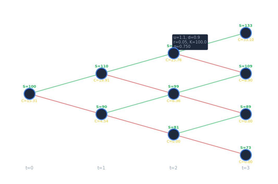
\[ S_{j+1}^{n+1} = u S_j^n \quad \text{(up move, probability } p\text{)} \]\[ S_j^{n+1} = d S_j^n \quad \text{(down move, probability } 1-p\text{)} \]

The key structural property is that an up followed by a down move, or a down followed by an up move, leads to the same node \(S_1^2 = ud S_0\). If we additionally assume \(d = 1/u\), this recombination property is exact, producing a non-drifting recombining tree. In a two-period lattice, for example, there are five nodes: \(S_0^0 = S_0\) at step 0; \(S_1^1 = u S_0\) and \(S_0^1 = d S_0\) at step 1; and \(S_2^2 = u^2 S_0\), \(S_1^2 = ud S_0\), \(S_0^2 = d^2 S_0\) at step 2. The recombination means the number of nodes at step \(n\) is only \(n+1\) rather than \(2^n\), a crucial computational savings.

More generally, the price at node \(j\) at time step \(N\) (expiry) can be written in closed form as

\[ S_j^N = u^j d^{N-j} S_0 \]

Given a binomial lattice satisfying the no-arbitrage condition \(d < e^{r \Delta t} < u\), any European option can be priced by backward induction through the lattice.

The Additive Log-Price Model and Random Walk

Logarithmic Returns

In finance it is common and natural to work with logarithmic returns rather than price levels. Define \(X_n = \log(S_n)\). The log return in the \((n+1)\)-th period is

\[ \Delta X_n = \log\left(\frac{S_{n+1}}{S_n}\right) \]

The simple return \((S_{n+1} - S_n)/S_n\) is approximately equal to the log return when returns are small, since \(\log(1 + x) \approx x\) for small \(x\). Thus

\[ \frac{S_{n+1} - S_n}{S_n} \approx \log\left(\frac{S_{n+1}}{S_n}\right) \]

The log price evolves additively:

\[ X_{n+1} = \log(S_{n+1}) = X_n + \Delta X_n \]

The Binomial Log-Return Distribution

In the binomial model, the log return in each period takes one of two values:

\[ \Delta X_n = \begin{cases} +\Delta h & \text{with probability } p \\ -\Delta h & \text{with probability } 1 - p \end{cases} \]

where \(\Delta h\) is a given positive constant. This is equivalent to the multiplicative model with \(u = e^{\Delta h}\) and \(d = e^{-\Delta h} = 1/u\), so the symmetric condition \(d = 1/u\) corresponds exactly to the up and down log returns being \(+\Delta h\) and \(-\Delta h\) respectively.

The cumulative log return over the first \(n\) periods is the sum \(\sum_{k=0}^{n-1} \Delta X_k\), and the log price at time \(t_n\) is

\[ X_n = X_0 + \sum_{k=0}^{n-1} \Delta X_k \]

This is precisely the position of a random walker starting at \(X_0\) (or at 0 if \(X_0 = 0\) who at each step moves up by \(\Delta h\) with probability \(p\) and down by \(\Delta h\) with probability \(1-p\). This additive model for the log price is far easier to analyze than the multiplicative model for the price itself.

Properties of the Discrete Random Walk

The discrete random walk formed by the log returns has three fundamental properties. First, each increment \(\Delta X_n\) has the same distribution for any \(n\), taking value \(+\Delta h\) with probability \(p\) and \(-\Delta h\) with probability \(1-p\). Second, the increments are independent: for \(n \neq n'\),

\[ \mathbf{E}(\Delta X_n \Delta X_{n'}) = \mathbf{E}(\Delta X_n)\mathbf{E}(\Delta X_{n'}) \]

This means the next price move is independent of all past moves — the process is Markovian (a random walk). Third, the statistical moments are determined by \(p\) and \(\Delta h\):

\[ \mathbf{E}(\Delta X_n) = p\Delta h - (1-p)\Delta h = (2p-1)\Delta h =: \alpha_0 \]\[ \mathbf{E}(\Delta X_n^2) = p(\Delta h)^2 + (1-p)(\Delta h)^2 = (\Delta h)^2 \]\[ \mathbf{var}(\Delta X_n) = (\Delta h)^2 - (2p-1)^2(\Delta h)^2 =: \sigma_0^2 \]

Convergence to the Normal Distribution via the Central Limit Theorem

By the Central Limit Theorem, as \(N \to \infty\) with the time step \(\Delta t = T/N\) shrinking, the normalized cumulative log return converges in distribution to a standard normal:

\[ \text{prob}\left(\frac{\sum_{n=0}^{N-1} \Delta X_n - N\alpha_0}{\sigma_0 \sqrt{N}} \leq x\right) \to F_{\text{normal}}(x) \]

where \(F_{\text{normal}}(x)\) is the cumulative distribution function (CDF) of the standard normal:

\[ F_{\text{normal}}(x) = \frac{1}{\sqrt{2\pi}} \int_{-\infty}^{x} e^{-s^2/2} \, ds \]

This convergence result is the continuous-time limit underpinning the Black-Scholes formula.

Constructing the Binomial Lattice: Choosing u, d, p

Matching the Statistical Moments of the Underlying

To use the binomial lattice as a model for a real stock, we need to choose the parameters \(u\), \(d\), and \(p\) so that the lattice correctly captures the statistical properties of the stock’s returns. Assume the underlying stock has two key annual statistics: the average log return per year \(\alpha\) and the volatility (standard deviation of the annual log return) \(\sigma\), so the variance of the annual log return is \(\sigma^2\).

Over a small interval \(\Delta t\), the expected log return is \(\alpha \Delta t\) and its variance is \(\sigma^2 \Delta t\). We choose the binomial parameters to match these two statistics simultaneously. Taking \(u = e^{\Delta h}\) and \(d = 1/u = e^{-\Delta h}\), the matching conditions become:

\[ \mathbf{E}(\Delta X_n) = p \Delta h - (1-p)\Delta h = \mathbf{E}\left[\log(S_{t+\Delta t}/S_t)\right] = \alpha \Delta t \]\[ \mathbf{var}(\Delta X_n) = (\Delta h)^2 - (2p-1)^2(\Delta h)^2 = \mathbf{var}\left[\log(S_{t+\Delta t}/S_t)\right] = \sigma^2 \Delta t \]

Since we have two equations and three unknowns (\(u\), \(d\), \(p\), there is a one-parameter family of solutions. One additional constraint is needed to pin down a unique choice.

The CRR Parameterization

A widely used choice, due to Cox, Ross, and Rubinstein (1979) and known as the CRR parameterization, is:

\[ u = e^{\sigma \sqrt{\Delta t}}, \qquad d = \frac{1}{u} = e^{-\sigma \sqrt{\Delta t}}, \qquad p = \frac{1}{2} + \frac{1}{2} \frac{\alpha}{\sigma} \sqrt{\Delta t} \]

Here \(\Delta h = \sigma \sqrt{\Delta t}\), meaning the step size in the log-price random walk scales as the square root of the time step. Several important observations follow from this construction.

First, the parameters \(u\) and \(d\) depend only on the volatility \(\sigma\), not on the drift \(\alpha\). The expected log return \(\alpha\) enters only through the real-world probability \(p\). But since we already know from Lecture 4 that \(p\) is irrelevant to option pricing, the drift \(\alpha\) plays no role in determining option values — option value depends on volatility only, not the expected rate of return.

Second, the CRR choice produces a recombining tree, since \(ud = 1\). This is illustrated by a two-period CRR lattice, where the five nodes take values \(S_0 e^{2\sigma\sqrt{\Delta t}}\), \(S_0\), and \(S_0 e^{-2\sigma\sqrt{\Delta t}}\) at the terminal step — the middle node \(S_0\) is reached by either an up-then-down or a down-then-up path.

Third, there are in principle many other valid parameterizations beyond CRR, since we have two moment-matching equations and three free parameters. However, one can also directly set up the lattice under the no-arbitrage (risk-neutral) measure, in which the expected rate of return is \(r\) and the probability is \(q^*\), rather than the real-world measure with drift \(\alpha\) and probability \(p\). Both approaches yield the same option prices.

Pricing European Options on the Binomial Lattice

The Four-Step Algorithm

Pricing a European option with expiry \(T\) on an \(N\)-period lattice proceeds in four steps.

Step 1: Choose parameters. Select \(u\), \(d\), and \(p\) to match the log-return statistics of the underlying. For the CRR choice, set \(\log(u) = \Delta h = \sigma \sqrt{\Delta t}\). Ensure \(\Delta t\) is sufficiently small that the no-arbitrage condition

\[ e^{-\sigma\sqrt{\Delta t}} \leq e^{r \Delta t} \leq e^{\sigma \sqrt{\Delta t}} \]

is satisfied. For the CRR lattice with \(\Delta t\) small, this condition holds automatically.

Step 2: Build the lattice of stock prices. Using \(u\) and \(d\), populate the lattice via the recurrence \(S_{j+1}^{n+1} = u S_j^n\) and \(S_j^{n+1} = d S_j^n\). The closed-form terminal prices are \(S_j^N = u^j d^{N-j} S_0\) for \(j = 0, 1, \ldots, N\).

Step 3: Compute terminal option values. At the expiry \(T = t_N\), set the option values to the payoff:

\[ V_j^N = \text{payoff}(S_j^N), \qquad 0 \leq j \leq N \]

For a European call this is \(\max(S_j^N - K, 0)\); for a put, \(\max(K - S_j^N, 0)\).

Step 4: Roll back through the lattice (backward induction). Working from \(n = N-1\) back to \(n = 0\), apply the one-step risk-neutral pricing formula at each node:

\[ V_j^n = e^{-r \Delta t} \left( q^* V_{j+1}^{n+1} + (1 - q^*) V_j^{n+1} \right), \qquad j = 0, 1, \ldots, n \]

where the risk-neutral probability is

\[ q^* = \frac{e^{r \Delta t} - d}{u - d} \]

After completing the backward sweep, \(V_0^0\) is the fair option price at time 0. An example MATLAB implementation of this algorithm (the “TreeSlow” code) is discussed in Section 5.5 of the course notes.

---

American Options, Dividends, Convergence, and the Black-Scholes Formula

Overview

Lecture 6 extends the binomial lattice framework in three directions: handling dividends paid by the underlying stock, pricing American options with their early-exercise feature, and analyzing the convergence of binomial lattice prices to the exact continuous-time limit known as the Black-Scholes formula.

European Option Pricing with Dividends

The Dividend Model

Many stocks pay dividends during the life of an option, and these payments affect the stock price and hence the option value. We model a single dividend payment occurring at a known future time \(t_d\) with \(0 \leq t_d \leq T\). Two time-point notations are useful: \(t_d^-\) denotes the instant immediately before the dividend payment, and \(t_d^+\) denotes the instant immediately after.

The dividend amount is \(D = \rho S(t_d^-)\), a fixed fraction \(\rho\) of the stock price just before the ex-dividend instant. Such a proportional dividend is the standard assumption in the binomial lattice framework.

Effect of the Dividend on the Stock Price

By the no-arbitrage principle, the stock price must drop by exactly the dividend amount at the dividend date. If it did not, one could buy the stock just before \(t_d\), collect the dividend, and sell immediately after, generating a riskless profit. Therefore:

\[ S(t_d^+) = S(t_d^-) - D \]

However, this drop in the stock price does not affect the option holder or writer, because the option is assumed to be dividend protected by contract. The option’s value is a continuous function of time at \(t_d\):

\[ V\left(S(t_d^-), t_d^-\right) = V\left(S(t_d^+), t_d^+\right) = V\left(S(t_d^-) - D, t_d^+\right) \]

This relationship is key: it says that the option value computed using the pre-dividend stock price equals the option value computed using the post-dividend (lower) stock price at the same instant. This continuity condition is used in the backward induction to handle the jump in the underlying.

Backward Induction Algorithm with Dividends

The pricing algorithm is modified as follows. Roll back through the lattice from \(n = N-1\) to \(n = 0\). At each interior step, apply the standard one-step discounting:

\[ V_j^n = e^{-\Delta t} \left( q^* V_{j+1}^{n+1} + (1 - q^*) V_j^{n+1} \right) \]

When the backward sweep reaches the time step \(t_n\) that is closest to the dividend date \(t_d\), an additional adjustment is applied. The option values \(V_j^n\) at time \(t_n^-\) are computed using the continuity condition (equation (1) above) and interpolation. The interpolation is necessary because \(S(t_d^-) - D\) will generally not coincide with any of the lattice node prices \(S_j^n\), so the option value at \(S(t_d^-) - D\) must be interpolated from neighboring node values.

Pricing American Options

The Early Exercise Problem

An American option differs from its European counterpart in that the holder may exercise it at any time up to and including expiry. Formally, the holder may exercise at any of the discrete times \(t_n\), \(n = 0, 1, \ldots, N\). At each node the holder faces a decision: exercise now and receive \(\text{payoff}(S_j^n)\), or continue to hold and receive the continuation value. The holder will rationally choose whichever is larger.

At expiry \(T = t_N\), the holder exercises if and only if the payoff is positive, so \(V_j^N = \text{payoff}(S_j^N)\) as before. The optimal exercise strategy must be optimal at every node, given that optimal decisions will be made at all subsequent nodes. This Bellman’s principle of dynamic programming means the problem can be decomposed into a sequence of single-step decisions solved in backward order.

Backward Induction with Early Exercise

The algorithm for pricing an American option is:

Terminal condition: At expiry, \(V_j^N = \text{payoff}(S_j^N)\) for \(j = 0, 1, \ldots, N\).

Backward recursion: For \(n = N-1, N-2, \ldots, 0\) and for each \(j = 0, 1, \ldots, n\), first compute the continuation value (the value of holding the option for one more step):

\[ (V_j^n)^* = e^{-r \Delta t} \mathbf{E}^Q(V^{n+1} | S_j^n) = e^{-r \Delta t} \left( q^* V_{j+1}^{n+1} + (1-q^*) V_j^{n+1} \right) \]

Then compare with the immediate exercise value to get the American option value at this node:

\[ V_j^n = \max\left( (V_j^n)^*, \text{payoff}(S_j^n) \right), \qquad j = 0, 1, \ldots, n \]

The optimal exercise strategy is to exercise immediately at node \((t_n, S_j^n)\) whenever the continuation value is less than the intrinsic (immediate exercise) value. After completing the backward sweep, \(V_0^0\) gives the fair American option price today.

The only algorithmic change from European pricing is the replacement of the direct assignment \(V_j^n = (V_j^n)^*\) with the max operation. This single modification correctly accounts for the early exercise premium that American options carry relative to European options.

Computational Costs

The backward induction algorithm over an \(N\)-period lattice has a total floating point operation count of \(O(N^2)\), since there are on the order of \(N^2/2\) nodes in the lattice. For time efficiency, the inner loop over node indices \(j\) can be vectorized in MATLAB or NumPy, replacing the explicit inner for-loop with array operations (see Section 2.5 of the course notes for a vectorized implementation). For space efficiency, if only the price \(V_0^0\) at time zero is needed (and not the full lattice of option values), the backward sweep can be carried out using \(O(N)\) storage by overwriting a one-dimensional array of length \(N+1\) at each step.

Convergence of the Binomial Lattice

Setting and Result

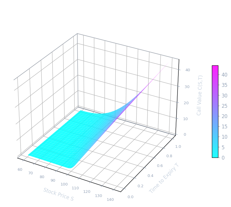
As \(N \to \infty\) (equivalently, \(\Delta t \to 0\), the binomial lattice option price converges to the exact continuous-time price. By the Central Limit Theorem, \(\log S_T - \log S_0\) converges to a normal distribution with mean \(\alpha T\) and variance \(\sigma^2 T\), which is the log-normal stock price model of Black and Scholes. It can be shown rigorously that the binomial lattice European option value functions converge to the Black-Scholes formulae.

Convergence Rate

Let \(V_0^{\text{exact}} = V(S_0, 0)\) denote the exact Black-Scholes price, and let \(V_0^{\text{tree}}(\Delta t)\) denote the binomial lattice price at time 0 with step size \(\Delta t = T/N\). PDE theory (discussed later in the course) shows that if the strike price falls exactly on a binomial lattice node, the error is linear in \(\Delta t\):

\[ V_0^{\text{tree}}(\Delta t) = V_0^{\text{exact}} + \text{const} \cdot \Delta t + \text{small } o(\Delta t) \]

Otherwise, when the strike does not align with a node, the convergence may be erratic and smoothing of the payoff is required (see Section 5.4 of the course notes for techniques to restore clean convergence).

Diagnosing Convergence Rate Computationally

If the convergence is linear in \(\Delta t\), then halving \(\Delta t\) should halve the error, and the ratio

\[ \lim_{\Delta t \to 0} \frac{V_0^{\text{tree}}(\Delta t / 2) - V_0^{\text{tree}}(\Delta t)}{V_0^{\text{tree}}(\Delta t / 4) - V_0^{\text{tree}}(\Delta t / 2)} \]

should approach 2. If the convergence is quadratic in \(\Delta t\), meaning

\[ V_0^{\text{tree}}(\Delta t) = V_0^{\text{exact}} + \alpha (\Delta t)^2 + o((\Delta t)^2) \]

for some constant \(\alpha\) independent of \(\Delta t\), then the same ratio would approach 4. This provides a practical computational test for verifying the order of convergence of any numerical method.

The Black-Scholes Formula

Derivation via the Central Limit Theorem

The continuous-time limit of the binomial lattice is the Black-Scholes model, in which the log price \(\log S_t\) follows a Brownian motion with drift. The Central Limit Theorem implies that \(\log S_t - \log S_0\) has a normal distribution with mean \(\alpha t\) and variance \(\sigma^2 t\). The binomial lattice option value converges to the Black-Scholes formula as \(N \to \infty\).

The Black-Scholes Formula for European Calls

For \(0 \leq t \leq T\), the Black-Scholes price of a European call option with current stock price \(S\), strike \(K\), risk-free rate \(r\), volatility \(\sigma\), and time to expiry \(T - t\) is

\[ C(S, t) = S \mathcal{N}_{cdf}(d_1) - K e^{-r(T-t)} \mathcal{N}_{cdf}(d_2) \]

where \(\mathcal{N}_{cdf}(d)\) is the cumulative distribution function of the standard normal:

\[ \mathcal{N}_{cdf}(d) = \frac{1}{\sqrt{2\pi}} \int_{-\infty}^{d} e^{-\frac{1}{2} y^2} \, dy \]

and the arguments \(d_1\) and \(d_2\) are given by

\[ d_1 = \frac{\log(S/K) + (r + 0.5\sigma^2)(T-t)}{\sigma \sqrt{T-t}} \]\[ d_2 = \frac{\log(S/K) + (r - 0.5\sigma^2)(T-t)}{\sigma \sqrt{T-t}} \]

Note that \(d_2 = d_1 - \sigma\sqrt{T-t}\). Here \(T - t\) is the time to expiry. The formula makes clear that the option price depends on the current stock price \(S\), the strike \(K\), the risk-free rate \(r\), the volatility \(\sigma\), and the time to expiry \(T - t\).

Key Properties of the Black-Scholes Formula

Two properties of the formula deserve special emphasis. First, consistent with the binomial model analysis, the option value depends only on the volatility \(\sigma\), not on the average rate of return \(\alpha\). The drift of the stock under the real-world measure is entirely irrelevant to the option price. Second, unlike the European option, there is no closed-form analytic formula for American option pricing in the Black-Scholes framework. American options must be priced numerically — for instance using the binomial lattice backward induction algorithm with the early-exercise modification — or by solving a partial differential equation with a free boundary.

Put-Call Parity and European Puts

The Black-Scholes formula for a European put can be derived either by direct computation or, more elegantly, from put-call parity. Put-call parity states that for European options on the same underlying with the same strike and expiry:

\[ C(S, t) - P(S, t) = S - K e^{-r(T-t)} \]

Rearranging and using the identity \(\mathcal{N}_{cdf}(-x) = 1 - \mathcal{N}_{cdf}(x)\) yields the European put price:

\[ P(S, t) = K e^{-r(T-t)} \mathcal{N}_{cdf}(-d_2) - S \mathcal{N}_{cdf}(-d_1) \]

The Black-Scholes formula represents the culmination of the binomial lattice approach: it is the analytic closed-form that the numerical lattice converges to as the number of time steps grows without bound, and it provides a benchmark against which computational methods can be validated.

Stochastic Calculus and the Black-Scholes Model

Standard Brownian Motion

From Discrete Random Walk to Continuous Process

The mathematical foundation of modern option pricing theory rests on the concept of standard Brownian motion, also called the Wiener process. To understand where this object comes from, it is helpful to begin with a discrete model and examine what happens as the time step shrinks to zero.

Consider a special binomial lattice, a discrete random walk starting at \( X_0 = 0 \). At each step, the increment \( \Delta X_n \) is a symmetric coin flip scaled by the square root of the time step:

\[ \Delta X_n = \begin{cases} \sqrt{\Delta t} & \text{with probability } p = 0.5 \\ -\sqrt{\Delta t} & \text{with probability } 0.5 \end{cases} \]

The choice to scale by \( \sqrt{\Delta t} \) rather than \( \Delta t \) is deliberate and essential: it ensures that the variance of the cumulative sum grows linearly with time, which is the signature property of Brownian motion. Now we take the continuous-time limit. As \( \Delta t \to 0 \), the discrete time step becomes the differential \( dt \), and the increment \( \Delta X_t \) becomes the infinitesimal \( dX_t \). The limit of this random walk is a continuous process, which is called standard Brownian motion and is conventionally denoted \( Z_t \).

Formal Properties

A standard Brownian motion \( Z_t \) is defined by three fundamental properties.

First, initialization: \( Z(0) = 0 \). The process starts at the origin.

Second, normally distributed increments: for all \( t \geq 0 \) and \( \Delta t > 0 \), the increment \( Z(t + \Delta t) - Z(t) \) is normally distributed with mean zero and variance \( \Delta t \):

\[ Z(t + \Delta t) - Z(t) \sim \mathcal{N}(0, \Delta t) \]

This says that over any time interval of length \( \Delta t \), the change in the Brownian motion is a zero-mean Gaussian random variable whose variance equals the length of the interval.

Third, independent increments: for any \( 0 \leq t_1 < t_2 \leq t_3 < t_4 \), the increments \( Z(t_2) - Z(t_1) \) and \( Z(t_4) - Z(t_3) \) are independent random variables. Non-overlapping increments carry no information about one another.

Two important consequences follow from these definitions. Taking \( t_1 = 0 \) in the second property, one sees that \( Z_t \sim \mathcal{N}(0, t) \): the process \( Z_t \) at any time \( t \) has a normal distribution with mean zero and variance \( t \). The independent-increments property is also known as the Markovian property: the future evolution of the process depends only on the current state, not on the full history. This is consistent with the efficient market hypothesis, which asserts that all past price information is already reflected in the current price.

More Properties: The Infinitesimal Increment

It is instructive to examine the structure of an infinitesimal increment of Brownian motion more carefully. Since \( \Delta Z_t = Z(t + \Delta t) - Z(t) \sim \mathcal{N}(0, \Delta t) \), we can write this increment as

\[ \Delta Z_t = \phi_t \sqrt{\Delta t} \quad \text{or equivalently} \quad dZ_t = \phi_t \sqrt{dt} \]

where \( \phi_t \sim \mathcal{N}(0,1) \) is an independent standard normal random variable at each time \( t \). Equivalently, \( dZ_t / dt = \phi_t / \sqrt{dt} \), which diverges as \( dt \to 0 \). This captures a fundamental regularity result: the standard Brownian motion \( Z_t = Z_0 + \int_0^t dZ_s \) is continuous but not differentiable. Its sample paths are nowhere smooth in the classical sense.

The moments of the standard normal \( \phi_t \) are:

\[ \mathbf{E}(\phi_t) = 0, \quad \mathbf{E}(\phi_t^2) = 1, \quad \mathbf{E}(\phi_t^3) = 0, \quad \mathbf{E}(\phi_t^4) = 3 \]

From these one computes the mean and variance of the squared increment \( (\Delta Z_t)^2 \):

\[ \mathbf{E}((\Delta Z_t)^2) = \mathbf{E}(\Delta t \cdot \phi_t^2) = \Delta t \cdot \mathbf{E}(\phi_t^2) = \Delta t \]\[ \mathbf{var}((\Delta Z_t)^2) = \mathbf{E}((\Delta Z_t)^4) - (\mathbf{E}((\Delta Z_t)^2))^2 = (\Delta t)^2 \mathbf{E}(\phi_t^4) - (\Delta t)^2 = O((\Delta t)^2) \]

A crucial observation: the variance of \( (\Delta Z_t)^2 \) goes to zero quadratically in \( \Delta t \). This means that as \( \Delta t \to 0 \), the squared increment \( (dZ_t)^2 \) becomes deterministic, concentrating on its expected value. We can therefore write the fundamental identity of stochastic calculus:

\[ (dZ_t)^2 = dt \]

This non-classical rule, where a stochastic differential squared equals a deterministic differential, is at the heart of Itô’s Lemma.

Summary of Important Properties of \( Z_t \)

To summarize the key operational facts: if \( \phi_t \sim \mathcal{N}(0,1) \), then

\[ \Delta Z_t = \phi_t \sqrt{\Delta t}, \quad dZ_t = \phi_t \sqrt{dt}, \quad (dZ_t)^2 = dt \]

These identities will be used repeatedly in deriving Itô’s Lemma and solving the Black-Scholes SDE.

---

Itô’s Process and the Stochastic Integral

Itô’s Process

A general Itô’s process \( X_t \) is a solution to the stochastic differential equation (SDE):

\[ dX_t = a \cdot dt + b \cdot dZ_t \]

where \( a \) and \( b \) can be constants or functions of \( (X_t, t) \). The term \( a \cdot dt \) is the deterministic trend component, governing the expected direction of movement, while \( b \cdot dZ_t \) is the random fluctuation component, encoding the uncertainty driven by the standard Brownian motion.

The Stochastic (Itô) Integral

Before turning to Itô’s Lemma, we need to define precisely what \( \int_0^T b(t) \, dZ_t \) means. In classical deterministic calculus, the integral \( \int_0^T f(t_n) \, dt \) is defined as the limit of Riemann sums, and the choice of evaluation point within each sub-interval (left endpoint, right endpoint, midpoint) does not matter in the limit because the integrand is smooth. Formally:

\[ \int_0^T f(t_n) \, dt = \lim_{N \to +\infty} \sum_{n=0}^{N-1} f(t_n) \Delta t = \lim_{N \to +\infty} \sum_{n=0}^{N-1} f(t_{n+1}) \Delta t \]

where \( t_n = n \Delta t \) and \( \Delta t = T/N \). For stochastic integrals, the situation is fundamentally different because the integrand \( b(t) \) and the integrator \( Z_t \) are both random and correlated, so the choice of evaluation point matters crucially in the limit.

The Itô integral is defined by evaluating the integrand at the left endpoint of each sub-interval:

\[ \int_0^T b(t) \, dZ_t = \lim_{N \to +\infty} \left( \sum_{n=0}^{N-1} b(t_n)(Z(t_{n+1}) - Z(t_n)) \right) \]

where the limit is taken in the mean square sense, meaning:

\[ \lim_{N \to +\infty} \mathbf{E}\left( \left( \sum_{k=0}^{N-1} b(t_{n+1})(Z(t_{n+1}) - Z(t_n)) - \int_0^T b(t) \, dZ_t \right)^2 \right) = 0 \]

Two notes are important here. First, the partial sum \( \sum_{n=0}^{N-1} b(t_n)(Z(t_{n+1}) - Z(t_n)) \) is a random variable, and so is the limiting Itô integral \( \int_0^T b(t) \, dZ_t \). Second, the left-endpoint convention is financially meaningful: it says that the trading position \( b(t_n) \) is determined using only information available up to time \( t_n \), before seeing the Brownian increment \( Z(t_{n+1}) - Z(t_n) \). Using the right-endpoint (which would yield a different answer) would correspond to using future information, which is not admissible in finance.

Solution for Constant Coefficients

As an analogy, recall that the bond price satisfies the deterministic ODE \( d\beta(\tau) = r \beta \, d\tau \), or equivalently \( d\log(\beta(\tau)) = r \, d\tau \). Integrating gives \( \beta(t) = \beta(0) e^{rt} \).

For the SDE \( dX_t = a \, dt + b \, dZ_t \) with constants \( a, b \), integrating directly gives:

\[ X(t) = X(0) + \int_0^t (a \, d\tau + b \, dZ(\tau)) = X(0) + a \cdot t + b \cdot Z_t \]

The solution is simply the initial value plus a linear trend plus a Brownian motion term scaled by \( b \). This is the simplest Itô process, sometimes called arithmetic Brownian motion.

---

Geometric Brownian Motion and the Black-Scholes Model

The GBM SDE

The Black-Scholes model for the stock price \( S_t \) is the Geometric Brownian Motion (GBM) model, a stochastic differential equation of the form:

\[ \frac{dS_t}{S_t} = \mu \, dt + \sigma \, dZ_t \]

or equivalently,

\[ dS_t = \mu S_t \, dt + \sigma S_t \, dZ_t \]

Here \( \mu \) is the drift (expected instantaneous rate of return) and \( \sigma \) is the volatility (standard deviation of returns per unit time), both treated as constants. This is an Itô process with \( a(S_t, t) = \mu S_t \) and \( b(S_t, t) = \sigma S_t \). The left-hand side \( dS_t / S_t \) is the instantaneous relative return, so the model says the return consists of a deterministic drift \( \mu \, dt \) and a random fluctuation \( \sigma \, dZ_t \). The central question is: how do we solve this SDE for \( S_t \)?

We cannot solve it the same way as the constant-coefficient case, because the coefficients depend on \( S_t \) itself. The correct tool is Itô’s Lemma.

---

Itô’s Lemma

Statement

Itô’s Lemma is the stochastic analogue of the chain rule. It tells us how a smooth function of an Itô process evolves over time. Suppose that \( S_t \) satisfies the general SDE:

\[ dS_t = a(S_t, t) \, dt + b(S_t, t) \, dZ_t \]

Let \( G(S, t) : \mathbb{R}^2 \to \mathbb{R} \) be a smooth (twice continuously differentiable) function. Then \( Y_t = G(S_t, t) \) is itself an Itô process, and it satisfies:

\[ dY_t = \left[ \frac{\partial G}{\partial t} + a(S_t, t) \frac{\partial G}{\partial S} + \frac{1}{2} b(S_t, t)^2 \frac{\partial^2 G}{\partial S^2} \right] dt + b(S_t, t) \frac{\partial G}{\partial S} \, dZ_t \]

For the Black-Scholes model specifically, \( a(S_t, t) = \mu S_t \) and \( b(S_t, t) = \sigma S_t \), so the formula specializes to the well-known form involving the option Greeks: a theta term, a delta term, and a gamma term.

Proof (Derivation)

The key step in understanding Itô’s Lemma is to perform a Taylor expansion of \( G \) and keep track of which terms survive in the limit \( \Delta t \to 0 \), using the special stochastic rules.

For notational simplicity, write \( a \equiv a(S_t, t) \) and \( b \equiv b(S_t, t) \). By Taylor expansion:

\[ \Delta Y_t = G(S_t + \Delta S_t, t + \Delta t) - G(S_t, t) = \frac{\partial G}{\partial S} \Delta S_t + \frac{\partial G}{\partial t} \Delta t + \frac{1}{2} \frac{\partial^2 G}{\partial S^2} (\Delta S_t)^2 + \frac{\partial^2 G}{\partial S \partial t} (\Delta S_t)(\Delta t) + O((\Delta t)^2) \]

Now, since \( dS_t = a \, dt + b \, dZ_t \) and \( dZ_t = O(\sqrt{dt}) \), the cross term satisfies \( \Delta S_t \Delta t = O((\Delta t)^{3/2}) \), which is negligible. After discarding this cross term, we have:

\[ \Delta Y_t \approx \frac{\partial G}{\partial S} \Delta S_t + \frac{\partial G}{\partial t} \Delta t + \frac{1}{2} \frac{\partial^2 G}{\partial S^2} (\Delta S_t)^2 + O((\Delta t)^{3/2}) \]

The crucial computation is \( (dS_t)^2 \):

\[ (dS_t)^2 = (a \, dt + b \, dZ_t)^2 = a^2 (dt)^2 + b^2 (dZ_t)^2 + 2ab \, dt \, dZ_t = b^2 \, dt \]

where we used the fundamental identity \( (dZ_t)^2 = dt \), together with \( (dt)^2 = 0 \) and \( dt \, dZ_t = 0 \) (both vanish faster than \( dt \) as \( \Delta t \to 0 \). Taking the limit \( \Delta t \to 0 \):

\[ dY_t = \frac{\partial G}{\partial t} dt + \frac{\partial G}{\partial S} dS_t + \frac{1}{2} \frac{\partial^2 G}{\partial S^2} b^2 \, dt \]

Substituting \( dS_t = a \, dt + b \, dZ_t \) and collecting terms:

\[ dY_t = \left[ \frac{\partial G}{\partial t} + a(S_t, t) \frac{\partial G}{\partial S} + \frac{1}{2} b(S_t, t)^2 \frac{\partial^2 G}{\partial S^2} \right] dt + b(S_t, t) \frac{\partial G}{\partial S} \, dZ_t \]

This is Itô’s Lemma. The extra term \( \frac{1}{2} b^2 \partial^2 G / \partial S^2 \) — the Itô correction term — has no analogue in ordinary calculus. It arises precisely because Brownian motion has non-zero quadratic variation, captured by \( (dZ_t)^2 = dt \). In classical calculus, all second-order terms vanish; in stochastic calculus, the second-order Brownian term survives.

---

Explicit Solution of the Black-Scholes SDE

Applying Itô’s Lemma to \( \log S_t \)

We now apply Itô’s Lemma to solve the GBM SDE. Consider the function \( G(S, t) = \log(S) \). Its partial derivatives are:

\[ \frac{\partial G}{\partial t} = 0, \quad \frac{\partial G}{\partial S} = \frac{1}{S}, \quad \frac{\partial^2 G}{\partial S^2} = -\frac{1}{S^2} \]

For the Black-Scholes model, recall \( a(S_t, t) = \mu S_t \) and \( b(S_t, t) = \sigma S_t \). Substituting into Itô’s Lemma:

\[ d \log(S_t) = \left[ 0 + \mu S_t \cdot \frac{1}{S_t} + \frac{1}{2} (\sigma S_t)^2 \cdot \left(-\frac{1}{S_t^2}\right) \right] dt + \sigma S_t \cdot \frac{1}{S_t} \, dZ_t \]\[ d \log(S_t) = \left( \mu - \frac{1}{2} \sigma^2 \right) dt + \sigma \, dZ_t \]

This is a remarkable simplification: the SDE for \( \log(S_t) \) has constant coefficients, so we can integrate it directly. Integrating from \( 0 \) to \( t \):

\[ \log(S_t) - \log(S_0) = \int_0^t \left(\mu - \frac{1}{2}\sigma^2\right) ds + \int_0^t \sigma \, dZ_s = \left(\mu - \frac{1}{2}\sigma^2\right) t + \sigma(Z_t - Z_0) \]

Exponentiating both sides yields the explicit solution of the Black-Scholes model:

\[ S_t = S_0 \, e^{(\mu - \frac{1}{2}\sigma^2)t + \sigma Z_t} \]

Interpretation and the Lognormal Distribution

This explicit formula has several important consequences. First, assuming \( S_0 > 0 \), the stock price \( S_t \) is always strictly positive, since it is the exponential of a real number. This is one of the key advantages of GBM over arithmetic Brownian motion, which can take negative values and is therefore unsuitable as a model for stock prices.

Second, \( S_t \) has a lognormal distribution. Since \( Z_t \sim \mathcal{N}(0, t) \), the exponent \( (\mu - \frac{1}{2}\sigma^2)t + \sigma Z_t \) is normally distributed with mean \( (\mu - \frac{1}{2}\sigma^2)t \) and variance \( \sigma^2 t \). Therefore \( \log(S_t/S_0) \) is Gaussian, making \( S_t \) lognormally distributed.

Third, notice the Itô correction: the drift in the log-return is \( \mu - \frac{1}{2}\sigma^2 \), not \( \mu \). The term \( -\frac{1}{2}\sigma^2 \) is purely a consequence of the nonlinearity of the exponential and the Itô correction from Itô’s Lemma. It implies that the median of \( S_t \) grows at rate \( \mu - \frac{1}{2}\sigma^2 \), while the mean \( \mathbf{E}[S_t] = S_0 e^{\mu t} \) grows at rate \( \mu \). The difference between the mean growth rate and the median growth rate is exactly the volatility penalty \( \frac{1}{2}\sigma^2 \), a reflection of Jensen’s inequality applied to the convex exponential function.

---

Monte Carlo Methods for Option Pricing

Risk-Neutral Valuation

From the Binomial Lattice to the Continuous Model

Monte Carlo (MC) simulation is one of the most powerful and general methods for pricing financial derivatives. To understand why it works, we begin by recalling the risk-neutral pricing framework established in the binomial lattice setting, and then carry it over to the continuous Black-Scholes world.

In the binomial lattice, the no-arbitrage condition implies the existence of a risk-neutral probability \( q^* \) such that:

\[ S(t_n) = e^{-r \Delta t} \mathbf{E}^Q(S(t_{n+1})) \]\[ V(S(t_n), t_n) = e^{-r \Delta t} \mathbf{E}^Q(V(S(t_{n+1}), t_{n+1})) \]

where \( \mathbf{E}^Q(\cdot) \) denotes the expectation using \( q^* \) and \( V(S, t) \) is the European option value function. From equation (1), we can write:

\[ E^Q\left(\frac{S(t_{n+1})}{S(t_n)}\right) = e^{r \Delta t} = 1 + r \Delta t + O((\Delta t)^2) \]

Rearranging:

\[ E^Q\left(\frac{S(t_{n+1}) - S(t_n)}{S(t_n)}\right) = r \Delta t + O((\Delta t)^2) \]

Taking \( \Delta t \to 0 \), this implies that the expected rate of return under the risk-neutral measure is \( r \), the risk-free rate. In fact, under the risk-neutral probability measure \( Q \), the stock price dynamics change from the real-world drift \( \mu \) to the risk-free rate \( r \):

\[ \frac{dS_t}{S_t} = r \, dt + \sigma \, dZ_t^Q \]

where \( Z_t^Q \) is a standard Brownian motion under \( Q \). The actual (real-world) stock price dynamics are:

\[ \frac{dS_t}{S_t} = \mu \, dt + \sigma \, dZ_t \]

It is essential to note that the superscript \( Q \) emphasizes that paths simulated under the risk-neutral measure are not the same as paths of the actual underlying price process. The two measures use different drifts, but the same volatility \( \sigma \).

The Continuous Risk-Neutral Pricing Formula

Under the continuous model, the risk-neutral pricing formula for a European option with payoff at expiry \( T \) is:

\[ V(S, t) = e^{-r(T-t)} \mathbf{E}^Q(\text{payoff}(S_T)) \]

where the expectation \( \mathbf{E}^Q(\cdot) \) assumes the underlying asset price follows the risk-neutral model \( dS_t / S_t = r \, dt + \sigma \, dZ_t^Q \). This formula is the cornerstone of modern derivatives pricing: the option value equals the expected discounted payoff under the risk-neutral measure. The real-world drift \( \mu \) does not appear in the pricing formula — only the risk-free rate \( r \) and the volatility \( \sigma \) matter.

---

Monte Carlo Pricing of European Options

The Basic MC Algorithm

The risk-neutral pricing formula suggests a direct numerical method. Using risk-neutral pricing at time zero:

\[ V(S_0, 0) = e^{-rT} \mathbf{E}^Q\left( \text{payoff}(S_T) \right) \]

we can approximate this expectation by generating \( M \) independent samples \( (S_T)^j, \, j = 1, \ldots, M \) of \( S_T \) under the risk-neutral model, and averaging the discounted payoffs:

\[ V(S_0, 0) \approx \frac{1}{M} \sum_{j=1}^{M} \left( e^{-rT} \text{payoff}((S_T)^j) \right) \]

Under the Black-Scholes model, this is especially convenient because we have the explicit solution under the risk-neutral measure:

\[ S_t = S_0 e^{(r - \frac{1}{2}\sigma^2)t + \sigma Z_t} \]

To generate \( M \) independent samples of \( S_T \), we exploit the fact that \( Z_T \sim \mathcal{N}(0, T) \), so \( Z_T \) can be written as \( \sqrt{T} \) times a standard normal. In Matlab notation:

\[ S_T = S_0 e^{(r - \frac{1}{2}\sigma^2)T + \sigma \cdot \sqrt{T} \cdot \text{randn}(M,1)} \]

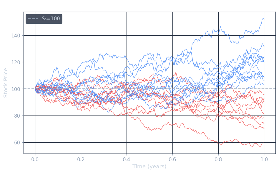
Here \( S_T \) is an \( M \)-by-1 vector of independent terminal prices. The i.i.d. samples \( \{(S_T)^j, \, j=1,\ldots,M\} \) can be generated directly from standard normals using the explicit formula, with no need to time-step through the path. This is a major advantage of having a closed-form solution: there is no time discretization error — the only source of error is the sampling error from using a finite \( M \).

---

Monte Carlo Pricing of Path-Dependent Options

What Are Path-Dependent Options?

A path-dependent option is one whose payoff depends not just on the terminal stock price \( S_T \), but on the entire price path \( S(t), \, 0 \leq t \leq T \). Because the payoff depends on the path, we cannot simply generate \( S_T \) directly — we must simulate the entire path at discrete time points.

A barrier option is a canonical example. It comes into existence or ceases to exist when the stock price crosses a specified barrier level. For instance, an up-and-out (Up-Out) barrier option: if \( S_t \) ever crosses an upper barrier \( S_u \), the option pays nothing; otherwise it pays the standard vanilla payoff. The existence of the option therefore depends on whether the price path has crossed the barrier.

To price options whose payoffs depend on the path, we simulate price paths \( S(t_n), \, n = 0, 1, \ldots, N \) by stepping forward through time. Using the exact BS formula for each time step (since the log-return over \( \Delta t \) is exactly Gaussian under constant \( \mu, \sigma \):

\[ S(t_{n+1}) = S(t_n) \cdot e^{(r - \frac{1}{2}\sigma^2)\Delta t + \sigma \cdot \sqrt{\Delta t} \cdot \text{randn}(M,1)} \]

This step-by-step simulation produces \( M \) complete price paths simultaneously, one for each of the \( M \) simulated scenarios.

Asian Options: A Worked Example

A classic example is the European Asian option, whose payoff is a function of the time-average of the stock price:

\[ \frac{1}{T} \int_0^T S_t \, dt \]

For example, an Asian call has payoff:

\[ \max\left( \frac{1}{T} \int_0^T S_t \, dt - K, \, 0 \right) \]

Asian options are popular because averaging dampens volatility and makes them harder to manipulate at expiry. For computational implementation, we discretize the integral. Let \( t_n = t_{n-1} + \Delta t \) and \( \Delta t = T/N \). Define the running average:

\[ A_n = \frac{1}{n} \sum_{k=1}^{n} S(t_k) \approx \frac{1}{t_n} \int_0^{t_n} S(\tau) \, d\tau \]

A useful recursion avoids storing the full sum at each step:

\[ A_n = \frac{1}{n}\left((n-1) A_{n-1} + S(t_n)\right) = \frac{n-1}{n} A_{n-1} + \frac{1}{n} S(t_n) \]

The full Monte Carlo algorithm in pseudocode is:

S_0 = S(0) * ones(M,1)
A_0 = 0
for n = 0, 1, ..., N-1
    A_{n+1} = n/(n+1) * A_n + 1/(n+1) * S_n
    S_{n+1} = S_n * exp((r - 0.5*sigma^2)*Delta_t + sigma*sqrt(Delta_t)*randn(M,1))
end
payoff = max(A_N - K, 0)
V_0 = exp(-rT) * mean(payoff)

Here all quantities are \( M \)-dimensional vectors, so each step simultaneously advances all \( M \) sample paths. The final option value is the discounted average of payoffs across all simulated paths.

---

Sampling Error in Monte Carlo Pricing

Why the Error Is \( O(1/\sqrt{M}) \)

When we use the explicit Black-Scholes formula to generate samples of \( S_T \) (with no time discretization), the only error in the MC estimate comes from the use of a finite number of samples \( M \). This is the sampling error. With \( M \) simulations, the sampling error is \( O(1/\sqrt{M}) \). Here is the precise argument.

Let \( Y^j = e^{-rT} \text{payoff}((S_T)^j) \) be the discounted payoff of the \( j \)-th simulation, where each \( Y^j \) is drawn independently from the same distribution as a random variable \( Y \). The Monte Carlo estimator is:

\[ V^M = \frac{Y^1 + \cdots + Y^M}{M} \]

This is an unbiased estimator of \( V_0 = \mathbf{E}(Y) \), since:

\[ \mathbf{E}(V^M) = \frac{1}{M} \sum_{j=1}^{M} \mathbf{E}(Y^j) = \mathbf{E}(Y) \]

The variance of the estimator is:

\[ \mathbf{var}(V^M) = \mathbf{E}\left(\left( \frac{Y^1 + \cdots + Y^M}{M} - \mathbf{E}(V^M) \right)^2 \right) = \frac{1}{M^2} \sum_{j=1}^{M} \mathbf{E}\left((Y^j - \mathbf{E}(Y))^2\right) = \frac{1}{M} \mathbf{var}(Y) \]

using independence of the \( Y^j \) and the fact that they are identically distributed. Therefore, the standard error of the MC estimator is:

\[ \text{std}(V^M) = \frac{1}{\sqrt{M}} \text{std}(Y) \]

By the Central Limit Theorem, as \( M \to +\infty \):

\[ V^M - \mathbf{E}(Y) \Longrightarrow \mathcal{N}\left(0, \frac{1}{\sqrt{M}} \sigma_Y \right) \]

where \( \sigma_Y = \text{std}(Y) \). Two important notes: the sampling error does not depend on the number of risky assets if the payoff function depends on multiple assets — this is why MC is particularly well-suited to high-dimensional problems (e.g., basket options on many underlyings). Additionally, \( V^M \) is itself a random quantity, since each \( Y^j \) is a random sample.

---

Confidence Intervals for MC Estimates

Constructing the Interval

In practice, the true standard deviation \( \sigma_Y \) is unknown. We estimate it from the sample using the sample standard deviation:

\[ \hat{\sigma} = \left[ \frac{\sum_{j=1}^{M} (Y^j - V^M)^2}{M-1} \right]^{1/2} \]

Approximating \( \sigma_Y \) by \( \hat{\sigma} \), the Central Limit Theorem gives:

\[ V^M - V_0 \approx \mathcal{N}\left(0, \frac{\hat{\sigma}}{\sqrt{M}}\right) \]

where \( V_0 = \mathbf{E}(Y) \) is the true option price.

The Normal Quantiles

For the standard normal distribution, given any confidence level \( \beta \), the interval \( [-x^*, x^*] \) satisfying

\[ \int_{-x^*}^{x^*} e^{-x^2/2} dx = \beta \]

where \( p(x) = e^{-x^2/2} \) is the standard normal density, can be determined from standard tables. Key facts:

• If \( \beta = 0.95 \), then \( x^* = 1.96 \).
• If \( \beta = 0.99 \), then \( x^* = 2.58 \).

Therefore, with 99% confidence, we can assert:

\[ V_0 \in \left[ V^M - \frac{2.58 \hat{\sigma}}{\sqrt{M}}, \; V^M + \frac{2.58 \hat{\sigma}}{\sqrt{M}} \right] \]

This confidence interval quantifies the uncertainty in the MC estimate. To halve the width of the interval (i.e., to halve the standard error), one must quadruple the number of simulations \( M \), since the error scales as \( 1/\sqrt{M} \). This slow convergence rate is an intrinsic feature of Monte Carlo methods, but the method compensates by being dimension-independent and extremely flexible in handling complex payoffs.

---

Monte Carlo Simulation — Euler Method and Dynamic Trading

Option Pricing Under the Generalized Black-Scholes Model

Review: Constant-Parameter BS Model

We begin by recalling the setting from Lecture 8. Under the standard Black-Scholes model with constant \( \mu \) and \( \sigma \), the stock price follows:

\[ \frac{dS_t}{S_t} = \mu \, dt + \sigma \, dZ_t \]

and by Itô’s Lemma we have the explicit solution:

\[ S_t = S_0 e^{(\mu - \frac{1}{2}\sigma^2)t + \sigma Z_t} \]

Under no-arbitrage, the fair value of a European option satisfies:

\[ V(S, t) = e^{-r(T-t)} \mathbf{E}^Q(\text{payoff}(S_T)) \]

where \( \mathbf{E}^Q(\cdot) \) is under the risk-neutral dynamics \( dS_t/S_t = r \, dt + \sigma \, dZ_t \). Since the explicit solution is available, sampling is easy: in Matlab, randn yields standard normal samples and thus \( S_T \) can be generated in one vectorized operation. A crucial benefit is that there is no time discretization error when the explicit formula is used — the only error is sampling error of order \( O(1/\sqrt{M}) \). We can also generate sample paths \( \{S(t_n), \, n=0,1,\ldots,N\} \) to price European path-dependent exotic options.

The Generalized BS Model: Local Volatility

In practice, the assumption of a constant volatility \( \sigma \) is often too restrictive. The Local Volatility Function (LVF) model, also called the generalized Black-Scholes model, replaces the constant \( \sigma \) with a function \( \sigma(S_t, t) \) that depends on both the current price and time:

\[ \frac{dS_t}{S_t} = r \, dt + \sigma(S_t, t) \, dZ_t \]

This is a much richer model — it can be calibrated to fit the observed market implied volatility surface, and it allows the volatility to be higher for lower stock prices (the so-called “volatility smile” or “skew” effect). However, the price we pay is that there is no explicit closed-form solution for \( S_t \) in general. We must discretize and simulate numerically. We can still price any European option (plain vanilla or exotic) using MC under the generalized BS model, though there will now be an additional time discretization error when numerical stepping is used.

---

The Euler Method for SDEs

Derivation of the Euler Time Step

The standard numerical method for simulating an SDE is the Euler method, the stochastic analogue of Euler’s method for ODEs. For the LVF model, divide the time interval \( [0, T] \) into \( N \) equal sub-intervals, with \( t_n = n \Delta t \), \( n = 0, 1, \ldots, N \), and \( \Delta t = T/N \).

Integrating the SDE over \( [t_n, t_{n+1}] \):

\[ \int_{t_n}^{t_{n+1}} dS_t = \int_{t_n}^{t_{n+1}} r S_t \, dt + \int_{t_n}^{t_{n+1}} \sigma(S_t, t) S_t \, dZ_t \]

The Euler approximation freezes the integrands at the left endpoint \( t_n \):

• The deterministic integral: \( \int_{t_n}^{t_{n+1}} r S_t \, dt \approx r S_n \Delta t \)
• The stochastic integral: \( \int_{t_n}^{t_{n+1}} \sigma(S_t, t) S_t \, dZ_t \approx \sigma(S_n, t_n) S_n \Delta Z(t_n) \)

Using \( \Delta Z(t_n) = \sqrt{\Delta t} \phi_n \) where \( \phi_n \sim \mathcal{N}(0,1) \) is independent at each step, we obtain the Euler discretization:

\[ S_{n+1} = S_n + S_n \left( r \Delta t + \sigma(S_n, t_n) \sqrt{\Delta t} \phi_n \right), \quad \phi_n \sim \mathcal{N}(0,1) \]

In the constant-\( \sigma \) case, this reduces to the familiar path-stepping formula used for Asian option pricing. In the LVF case, the local volatility \( \sigma(S_n, t_n) \) is evaluated at the current simulated price and time — this is what makes the Euler method straightforward to implement even for complex volatility surfaces.

---

Error Analysis of the Euler Method

Weak Convergence

The Euler method introduces a time discretization error in addition to the unavoidable sampling error. The accuracy of the Euler method is characterized in terms of weak convergence: for a time stepsize \( \Delta t \), the error in expected values satisfies:

\[ \left| \mathbf{E}(S(T)) - \mathbf{E}(S_T^{\Delta t}) \right| \leq C \Delta t \]

where \( S(T) \) is the exact solution to the SDE and \( S_T^{\Delta t} \) is the Euler approximation with step size \( \Delta t \), and \( C \) is a constant that does not depend on \( \Delta t \). Weak convergence is first-order in \( \Delta t \): halving the time step halves the discretization error. Further details can be found in Section 4.8.2 of the course notes.

Balancing Time Stepping Error and Sampling Error

When using the Euler method for option pricing, the total error has two components. The time discretization error is \( O(\Delta t) \), and the sampling error (from using \( M \) simulations) is \( O(1/\sqrt{M}) \):

\[ \text{total error} = O(\Delta t) + O\left(\frac{1}{\sqrt{M}}\right) \]

If we want the total error to be \( O(\Delta t) \) — meaning the sampling error should not dominate — we need \( 1/\sqrt{M} = O(\Delta t) \), which implies we should choose:

\[ M \approx \frac{\text{constant}}{(\Delta t)^2} \]

Computational Complexity

With this choice of \( M \), the total computational complexity of the MC method is:

\[ \text{complexity} = O(\text{#time steps} \times \text{#samples}) = O\left(\frac{T}{\Delta t} \cdot M\right) = O\left(\frac{M}{\Delta t}\right) \]

Substituting \( M = O(1/(\Delta t)^2) \):

\[ \text{complexity} = O\left(\frac{1}{(\Delta t)^3}\right) \]

Inverting, \( \Delta t = O(1 / \text{complexity}^{1/3}) \). Since the Euler error is \( O(\Delta t) \), we conclude:

\[ \text{error} = O(\Delta t) = O\left(\frac{1}{\text{complexity}^{1/3}}\right) \]

This means that to reduce the error by a factor of 10, we must increase the computational effort by a factor of \( 10^3 = 1000 \). The convergence rate of \( O(1/\text{complexity}^{1/3}) \) is relatively slow, which motivates research into variance reduction techniques and higher-order discretization methods such as the Milstein scheme.

---

How Efficient Is MC Option Pricing?

To put the efficiency of the MC method in perspective, we should ask: how much computational work is needed to achieve a prescribed accuracy? We have seen that the computational complexity scales as \( O(M / \Delta t) \), and the error decays as \( O(1/\text{complexity}^{1/3}) \). This is the fundamental efficiency tradeoff for the Euler-based MC method applied to the generalized BS model. In contrast, for the standard constant-parameter BS model, the explicit formula eliminates the time discretization error entirely, leaving only the sampling error at rate \( O(1/\sqrt{M}) \) — a significantly better convergence rate in terms of the number of samples alone.

---

Dynamic Trading Hedging Analysis via MC Simulation

Motivation: Beyond Pricing

Monte Carlo simulation is not limited to computing option prices. It is equally powerful for analyzing the performance of complex dynamic trading strategies, which is crucial for risk management at financial institutions. In this section we consider the application to dynamic hedging analysis.

In continuous-time theory, a perfectly hedged portfolio replicates the option payoff exactly. In practice, however, hedging is a dynamic trading process and portfolio rebalancing can only be implemented at discrete times — not continuously. The question of how well a discrete-time hedging strategy approximates the ideal continuous hedge, and how much residual risk remains, is an important practical problem that MC simulation is ideally suited to address.

Setup: Model-Based Hedging Analysis

We conduct a model-based hedging analysis based on the assumption that the stochastic model is correct. The scenario we consider is as follows: we are selling an option and simultaneously dynamically trading the underlying asset, with a cash account providing financing. This corresponds to a self-financed dynamic trading strategy:

\[ \{-V_t, \, \delta_t S_t, \, B_t\} \]

where \( -V_t \) denotes the short position in the option (value received from selling), \( \delta_t S_t \) is the value of the stock position (holding \( \delta_t \) shares), and \( B_t \) is the bond account balance. The bond account ensures that the portfolio is always self-financed — cash flows from buying and selling shares are exactly offset by the bond account, so no external capital is ever injected or withdrawn.

Goals of the Analysis

The central questions of hedging analysis are:

1. How good is the hedging/trading strategy? Does the portfolio track the option value closely?
2. How risky is it? How much risk (residual exposure) remains after hedging?
3. How do we measure the risk? What metrics best capture the distribution of hedging profit and loss (P&L)?

In addition to historical back-testing (which uses actual past price data), we can perform hedging analysis based on a stochastic model by generating many simulated price paths under the assumed model and running the hedging strategy on each path. By examining the distribution of the terminal hedging P&L across many simulated paths, we can characterize the risk and effectiveness of the strategy under the assumed model dynamics. This model-based approach is a fundamental component of risk management practice at banks and other financial institutions.

Connecting to MC Simulation

The MC framework makes this analysis tractable. For each of the \( M \) simulated price paths, we:

1. Simulate the stock price path \( S(t_n), \, n = 0, 1, \ldots, N \) using the Euler method (or the exact formula under constant BS).
2. At each time step \( t_n \), compute the hedge ratio \( \delta_{t_n} \) (e.g., the Black-Scholes delta) and rebalance the portfolio.
3. Track the bond account \( B_t \) to maintain self-financing.
4. At expiry \( T \), compute the terminal P&L = value of hedging portfolio minus option payoff.

Repeating across all \( M \) paths yields a sample distribution of the hedging P&L. Under perfect continuous hedging, the P&L would be zero for every path. The spread of the simulated P&L distribution across paths quantifies the hedging error arising from discrete rebalancing — this is the residual risk that the hedger must bear in practice. Tighter rebalancing schedules (smaller \( \Delta t \) reduce this risk but increase transaction costs, creating a fundamental tradeoff that can also be studied via MC simulation.

Dynamic Hedging — Delta, Gamma, and Vega

Dynamic Hedging (Trading) Analysis

The Black-Scholes framework assumes that the underlying asset price follows a geometric Brownian motion. Under this model the stock price dynamics are governed by the stochastic differential equation

\[ \frac{dS}{S} = \mu \, dt + \sigma \, dZ_t \]

where \( \mu \) is the drift, \( \sigma \) is the volatility, and \( Z_t \) is a standard Brownian motion. The central question of dynamic hedging is: given that a financial institution has written an option and therefore holds a short option position \( -V(S,t) \), how can it manage the resulting risk through continuous trading in the underlying asset?

The analysis begins by discretising time. We assume that trading is only permitted at times \( t_n = n\Delta t \), where \( \Delta t = T/N \), so that the trading dates form a uniform partition

\[ 0 = t_0 < t_1 < \cdots < t_N = T. \]

Between consecutive trading dates \( (t_n, t_{n+1}] \) the hedger holds a fixed number \( \delta_n \) of shares of the underlying asset. The hedging ratio \( \delta_n \) is chosen at time \( t_n \) based on information available at that moment, and is then kept constant until the next rebalancing date.

Delta Hedging and the Binomial Lattice Approximation

When a binomial lattice is employed to price the option, the delta at node \( (n, j) \) — that is, at time \( t_n \) and underlying price \( S^n_j \) — is computed as the ratio of the change in option value to the change in stock price across the two branches emanating from that node:

\[ \delta^n_j = \frac{V^{n+1}_{j+1} - V^{n+1}_j}{(u - d)S^n_j} \approx \frac{\partial V}{\partial S}(S^n_j, t_n). \]

Here \( u \) and \( d \) are the up- and down-factors of the binomial tree, and \( V^{n+1}_{j+1} \), \( V^{n+1}_j \) are the option values at the two successor nodes. This finite-difference ratio is precisely the first-order approximation to the partial derivative \( \partial V / \partial S \). More generally, regardless of the pricing method used, the number of units of the underlying held at time \( t_n \) is

\[ \delta_n = \frac{\partial V}{\partial S}(S_n, t_n). \]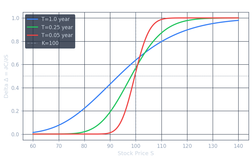

An important practical note concerns the simulation of underlying price paths for the purpose of evaluating hedging performance. When generating paths to assess the profit and loss (P&L) of the dynamic trading strategy, one uses the real-world drift \( \mu \), not the risk-neutral drift \( r \). This is a critical distinction: the risk-neutral measure is used purely for pricing, whereas analysis of actual hedging performance must reflect the real probability distribution of stock price moves.

Portfolio Construction and Rebalancing

The dynamic hedging portfolio is constructed to offset the short option position. Initially, at \( n = 0 \), the institution is short the option (value \( -V_0 = -V(S_0, 0) \), holds \( \delta_0 \) units of the stock, and places the residual in a cash account so that the initial portfolio value is zero. The cash balance at inception is therefore

\[ B_0 = V_0 - \delta_0 S_0. \]

The total portfolio value at any trading date \( t_n \) is

\[ \Pi_n = -V(S_n, t_n) + \delta_n S_n + B_n. \]

The portfolio \( \Pi = \{-V,\, \delta \cdot S,\, B\} \) consists of the short option, the stock holding, and the cash account.

Over the interval \( [t_n, t_{n+1}) \) the cash account grows at the risk-free rate. At time \( t_{n+1} \), just before rebalancing, the portfolio value is

\[ -V(S_{n+1}, t_{n+1}) + \delta_n S_{n+1} + B_n e^{r\Delta t}. \]

Rebalancing at \( t_{n+1} \) means adjusting the stock position from \( \delta_n \) to \( \delta_{n+1} \) without changing the portfolio value (the rebalancing condition \( \Pi_{t^-_{n+1}} = \Pi_{t^+_{n+1}} \). This forces the new cash balance to satisfy

\[ B_{n+1} = B_n e^{r\Delta t} + (\delta_n - \delta_{n+1})S_{n+1}. \]

The interpretation is immediate: if \( \delta_{n+1} > \delta_n \), additional shares must be purchased and the cost is debited from the cash account; if \( \delta_{n+1} < \delta_n \), shares are sold and the proceeds are credited to the cash account. At expiry \( t_N = T \), the portfolio formed at \( t_{N-1} \) is liquidated, yielding the terminal portfolio value

\[ \Pi_N = -V(S_N, t_N) + \delta_{N-1} S_N + B_{N-1} e^{r\Delta t}. \]

Profit and Loss Analysis

The terminal value \( \Pi_N \) is a random variable because it depends on the particular path taken by the stock price. Three qualitative outcomes are possible: if \( \Pi_N \equiv 0 \) along every path, the hedge is perfect; if \( \Pi_N > 0 \), the hedger realises a profit on that scenario; and if \( \Pi_N < 0 \), the hedger incurs a loss. In practice, a continuous-time delta hedge under the Black-Scholes model would be perfect, but because trading occurs only at discrete times, residual errors accumulate.

The quantity \( \Pi_N \) is therefore called the hedging error. To compare performance across options of different values, it is natural to normalise. The discounted relative P&L is defined as

\[ P&L = \frac{e^{-rT}\Pi_N}{V(S_0, 0)}. \]

One examines the full distribution of this P&L across Monte Carlo scenarios: its mean, standard deviation, and tail quantiles. A fundamental question is whether the P&L is zero along every individual scenario path. In general it is not, even under the Black-Scholes model, because the discrete-time rebalancing introduces a discretisation error proportional to \( \sqrt{\Delta t} \).

Computing Delta When Pricing by Monte Carlo

When option prices are computed by Monte Carlo rather than by an analytic formula or a lattice, obtaining the delta requires some care. The naive finite-difference approximation is

\[ \frac{\partial V}{\partial S}(S_0, 0) \approx \frac{V(S_0 + \Delta S, 0) - V(S_0, 0)}{\Delta S}. \]

Each option value is estimated by discounted expected payoff:

\[ \frac{\partial V}{\partial S}(S_0, 0) \approx e^{-r\Delta T} \frac{\text{mean}(\text{payoff}(S(T)|_{S_0+\Delta S})) - \text{mean}(\text{payoff}(S(T)|_{S_0}))}{\Delta S}. \]

The statistical error in each Monte Carlo mean is of order \( O(1/\sqrt{M}) \), where \( M \) is the number of sample paths. The error in the finite-difference approximation to \( \partial V/\partial S \) is therefore of order \( O(1/(\sqrt{M}\,\Delta S)) \). This creates a fundamental tension: making \( \Delta S \) small improves the finite-difference approximation but amplifies the statistical noise, requiring a very large number of paths. Indeed, for small \( \Delta S \), it can be difficult even to obtain the correct sign of the delta from naive independent simulations.

The standard remedy is to use the same set of random samples \( \phi \) for both simulations, so that the sampling errors partially cancel in the difference. Under the Black-Scholes model the procedure is:

\[ \phi = \text{randn}(M,1), \quad S_T = S_0 e^{(r-0.5\sigma^2)T + \sigma\sqrt{T}\phi}, \quad \tilde{S}_T = (S_0+\Delta S)e^{(r-0.5\sigma^2)T+\sigma\sqrt{T}\phi}. \]

The two option prices are then estimated as

\[ V_0 = e^{-rT}\text{mean}(\text{payoff}(S_T)), \quad \tilde{V}_0 = e^{-rT}\text{mean}(\text{payoff}(\tilde{S}_T)), \]

and the delta is

\[ \delta_0 = \frac{\tilde{V}_0 - V_0}{\Delta S}. \]

Because the same random draws \( \phi \) drive both stock price processes, the two payoff averages are highly correlated, and their difference has a much smaller variance than the difference of two independent estimates. This common random numbers technique is essential for stable delta estimation via Monte Carlo.

Delta-Neutral Hedging

Delta-neutral hedging is the strategy of choosing \( \delta_t = \partial V/\partial S(S_t, t) \) so that the hedged portfolio \( \Pi = \{-V,\, \delta \cdot S,\, B\} \) satisfies

\[ \frac{\partial \Pi}{\partial S} = -\frac{\partial V}{\partial S}(S,t) + \delta \equiv 0. \]

By matching the option’s delta, the portfolio is rendered insensitive to first-order movements in the underlying. In other words, delta hedging eliminates the linear exposure of the option value to changes in \( S \). However, because the option value is a nonlinear function of \( S \), first-order cancellation is insufficient when stock price moves are large. The residual sensitivity to curvature is captured by the gamma, defined as the second partial derivative \( \partial^2 V / \partial S^2 \).

Delta and Gamma Neutral Hedging

To hedge both the first- and second-order sensitivities simultaneously, one requires the portfolio to satisfy

\[ \frac{\partial \Pi}{\partial S} = 0 \quad \text{and} \quad \frac{\partial^2 \Pi}{\partial S^2} = 0 \]

at time \( t \). The underlying stock itself has zero gamma (it is linear in \( S \), so adding more stock cannot neutralise gamma. One must introduce an additional instrument \( I \) — for example, a liquidly traded vanilla option on \( S \) — that has nonzero gamma \( \partial^2 I/\partial S^2 \neq 0 \). The extended portfolio is

\[ \Pi = \{-V,\, \delta_S \cdot S,\, \delta_I \cdot I,\, B\}. \]

The delta-neutrality and gamma-neutrality conditions become the two-equation system

\[ -\frac{\partial V}{\partial S} + \delta_S + \delta_I \frac{\partial I}{\partial S} = 0, \]\[ -\frac{\partial^2 V}{\partial S^2} + \delta_I \frac{\partial^2 I}{\partial S^2} = 0. \]

(Note that stock holdings \( \delta_S \) do not appear in the second equation because the stock has zero gamma.) From the gamma equation one reads off the required holding in the additional instrument:

\[ \delta_I = \frac{\partial^2 V/\partial S^2}{\partial^2 I/\partial S^2}. \]

With \( \delta_I \) determined, one substitutes back into the delta equation to find \( \delta_S \). This two-instrument approach neutralises both the linear and quadratic responses of the portfolio to stock price movements, providing a much tighter hedge than delta alone, particularly when the stock makes large moves over a rebalancing interval.

Vega Hedging

Under the Black-Scholes model, the only parameter that is not directly observable in the market is the volatility \( \sigma \). All other inputs — the current stock price, the risk-free interest rate, the strike, and the time to maturity — are either directly quoted or can be read from standard financial data. The volatility must be estimated or implied from market prices. Because \( \sigma \) is uncertain, the option value is sensitive to errors in its specification, and this sensitivity is measured by the vega, defined as

\[ \text{vega} = \frac{\partial V}{\partial \sigma}. \]

A hedger who wishes to insulate the portfolio against unexpected changes in volatility must construct a vega-neutral portfolio. Because the underlying stock has zero vega (its price does not depend on \( \sigma \) directly), neutralising vega again requires a second option. The construction parallels the gamma-neutrality argument: one adds a position in a liquidly traded option \( I \) such that the portfolio’s total vega is zero, then adjusts the stock holding to restore delta neutrality. In this way one can simultaneously achieve delta and vega neutrality, or even delta, gamma, and vega neutrality, by introducing two additional option instruments.

Under the Black-Scholes model it can be shown that for both European calls \( C \) and puts \( P \) the vega is the same and equals

\[ \text{vega} = \frac{\partial C}{\partial \sigma} = \frac{\partial P}{\partial \sigma} = \frac{\mathcal{N}'(d_1)}{\sigma S_0 \sqrt{T}}, \]

where \( \mathcal{N}'(d) = \frac{1}{\sqrt{2\pi}} e^{-\frac{1}{2}d^2} \) is the standard normal density evaluated at \( d_1 \). Since \( \mathcal{N}'(d_1) > 0 \) for all finite \( d_1 \), vega is strictly positive for both calls and puts: option values are always increasing in volatility. This strict monotonicity — the option price as a function of \( \sigma \) is strictly increasing on \( (0, +\infty) \) — is a key property that underpins the uniqueness of implied volatility.

Risk, P&L Distributions, and the Role of Volatility

In a Black-Scholes model, \( \sigma \) represents the risk of the underlying, and the modelling assumption is that log-returns are approximately normally distributed. A natural follow-on question is: what does the distribution of the P&L look like under dynamic trading? Equivalently, what is the distribution of the call option terminal value \( V_T \)?

When a portfolio involves derivative instruments, the distribution of the resulting P&L is typically asymmetric and far from normal. Options introduce convexity into payoffs, so the P&L distribution inherits a skewed or heavy-tailed character. This asymmetry is precisely what motivates the use of specialised risk measures rather than simply reporting mean and standard deviation. For a portfolio \( \Pi \) of option positions, one wishes to compute the risk in \( P&L = \Pi_t - \Pi_0 \) over a short horizon \( t \) — for example, one trading day \( t = 1/250 \) of a year. The non-normality of this distribution motivates the risk measures examined in the next lecture.

---

Risk Measures, VaR, CVaR, and Implied Volatility

Risk Measures: Motivation

Financial markets have historically experienced severe crashes roughly once per decade — the 1987 Black Monday crash and the 2008 global financial crisis are prominent examples. Financial institutions often hold complex instruments such as options whose P&L distributions are far from normal, and whose losses in extreme scenarios can vastly exceed what a naive standard-deviation-based risk estimate would suggest. The central practical question is: what happens if the worst scenarios occur?

Alan Greenspan, then Chairman of the Federal Reserve, articulated this concern at the Joint Central Bank Research Conference in 1995: “Improving the characterization of the distribution of extreme values is of paramount importance.” This statement encapsulates the motivation for tail-risk measures that go beyond the mean and variance of the P&L distribution.

Value-at-Risk

Value-at-Risk (VaR) was first introduced in the aftermath of the 1987 crash, originating from the Weatherstone (then JP Morgan CEO) “4:15 report” — a daily one-page summary of the firm’s total risk. VaR is an extension of the notion of minimum profit (or equivalently maximum loss), and it is also frequently defined in terms of loss, where loss \( = -P&L \).

Precisely, VaR describes the predicted minimum profit (equivalently, the maximum loss) with a specified probability confidence level \( \beta \) over a certain time horizon. VaR is a percentile of the P&L distribution. It allows a risk manager to state, for example: “With 95% confidence, the minimum profit (maximum loss) over the next week is \( \cdots \).”

Formally, if \( p(x) \) is the probability density of P&L (whose explicit form is typically unknown for complex portfolios), then \( \text{VaR}_\beta \) satisfies either of the equivalent conditions

\[ \int_{-\infty}^{\text{VaR}} p(x)\,dx = 1 - \beta \quad \text{or} \quad \int_{\text{VaR}}^{\infty} p(x)\,dx = \beta. \]

The interpretation is that with probability \( \beta\% \), the P&L is at least \( \text{VaR} \). When the P&L distribution is plotted as a loss distribution (i.e., \( -P&L \), the VaR and CVaR appear at the right tail; with respect to the P&L distribution itself, they appear at the left tail.

For a discrete set of scenarios, \( \text{VaR}_\beta \) is the maximum P&L value \( x \) such that

\[ \text{Prob}(P&L \leq x) \leq 1 - \beta. \]

Conditional Value-at-Risk

One serious deficiency of VaR is that it provides no information about the magnitude of losses beyond the quantile threshold. Knowing that losses exceed VaR with probability \( 1-\beta \) says nothing about how bad those losses are — “What happens to the worst 5% of outcomes?” is a question that VaR cannot answer.

Conditional Value-at-Risk (CVaR), also called Expected Shortfall, addresses this gap. Assuming that the P&L distribution is continuous, CVaR is defined as the average P&L conditional on P&L being at most \( \text{VaR}_\beta \):

\[ \text{CVaR}_\beta = \mathbf{E}(P&L \mid P&L \leq \text{VaR}_\beta). \]

The interpretation is that CVaR is the expected P&L given that we are experiencing the worst \( 1 - \beta \) fraction of scenarios. It captures not just the threshold but the average severity of tail losses. A technical revision to this definition is required when the P&L distribution is discontinuous (for example, when dealing with discrete scenario sets), but the intuition remains the same.

VaR versus CVaR

A natural question is which risk measure — VaR or CVaR — is preferable. The answer from both theoretical and regulatory perspectives increasingly favours CVaR. CVaR is a coherent risk measure in the sense of Artzner et al. (1999), whereas VaR is not. The main difference concerns convexity: CVaR satisfies

\[ \text{CVaR}(\alpha \cdot \Pi + (1-\alpha) \cdot \hat{\Pi}) \leq \alpha \cdot \text{CVaR}(\Pi) + (1-\alpha) \cdot \text{CVaR}(\hat{\Pi}) \]

for any portfolios \( \Pi, \hat{\Pi} \) and \( 0 \leq \alpha \leq 1 \). This convexity property means that diversification is always rewarded: the CVaR of a mixture of two portfolios is no larger than the weighted average of their individual CVaRs. VaR lacks convexity, which means that a diversified portfolio can in theory have a higher VaR than the sum of its components — a perverse property that undermines its use as a basis for risk limits. Regulation based on both VaR and CVaR has been imposed on financial institutions.

Computing Scenario VaR and CVaR

In practice the P&L distribution is not known analytically, and one relies on Monte Carlo simulation. Given \( M \) independent P&L samples \( \{P&L_i,\, i = 1, \ldots, M\} \), the procedure is as follows.

First, sort the samples in ascending order so that \( P&L_1 < P&L_2 < \cdots < P&L_M \). Next, identify the largest index \( i_\beta \) such that

\[ \frac{i_\beta}{M} \leq 1 - \beta, \quad \text{equivalently,} \quad i_\beta = \lfloor (1-\beta) \cdot M \rfloor. \]

The scenario VaR is then

\[ \text{VaR}_\beta = P&L_{i_\beta}, \]

that is, the \( i_\beta \)-th order statistic. The scenario CVaR is the average of the \( i_\beta \) worst outcomes:

\[ \text{CVaR}_\beta = \frac{1}{i_\beta}(P&L_1 + \cdots + P&L_{i_\beta}). \]

As a concrete example, consider \( M = 1000 \) paths and a confidence level of \( \beta = 95\% \). Then \( i_{5\%} = \lfloor 0.05 \times 1000 \rfloor = 50 \), so

\[ \text{VaR}_{95\%} = P&L_{50}, \quad \text{CVaR}_{95\%} = \frac{1}{50}(P&L_1 + \cdots + P&L_{50}). \]

This scenario approach is widely used in industry, and regulatory capital requirements have been imposed based on both VaR and CVaR computed in precisely this manner.

Model Uncertainty and Vega Risk

Even if all market inputs are observed without error, the Black-Scholes model depends on a volatility parameter \( \sigma \) that must be estimated. The option Greeks measure the sensitivity of the option value to the underlying price and to model parameters. The three primary Greeks are:

• Delta: \( \partial V / \partial S \), the sensitivity to the stock price.
• Gamma: \( \partial^2 V / \partial S^2 \), the second-order sensitivity to the stock price.
• Vega: \( \partial V / \partial \sigma \), the sensitivity to the volatility.

Under the Black-Scholes model, the vega for both European calls and puts is

\[ \text{vega} = \frac{\partial C}{\partial \sigma} = \frac{\partial P}{\partial \sigma} = \frac{\mathcal{N}'(d_1)}{\sigma S_0 \sqrt{T}}, \quad \text{where} \quad \mathcal{N}'(d) = \frac{1}{\sqrt{2\pi}} e^{-\frac{1}{2}d^2}. \]

Since \( \mathcal{N}'(d_1) > 0 \) always, vega is strictly positive for all options under the Black-Scholes model. Consequently, the option value as a function of volatility \( \sigma \) is strictly monotonically increasing on \( \sigma \in (0, +\infty) \). This strict monotonicity is not just a curiosity — it implies that the mapping from volatility to option price is invertible, which is the foundation for implied volatility.

Implied Volatility

Assume that today’s market option price \( V_{\mathrm{mkt}} \) is observed. The market price encodes information about the market’s collective expectation of future volatility of the underlying. Since the Black-Scholes formula gives a one-to-one mapping between \( \sigma \) and the option price (for fixed all other parameters), one can invert this relationship. The implied volatility \( \check{\sigma} \) is defined as the volatility that, when plugged into the Black-Scholes formula, reproduces the observed market price:

\[ V_{\mathrm{BS}}(\sigma) = V_{\mathrm{mkt}}. \]

It can be shown that a unique positive implied volatility exists if and only if the market option price lies in the range of the Black-Scholes price as a function of \( \sigma \). For a European call, this means the market price must satisfy

\[ \max(0,\, S_0 - Ke^{-rT}) \leq C_{\mathrm{mkt}} < S_0. \]

Implied volatility is important for several reasons. It tells a trader the volatility that the option market is pricing in over the remaining life of the option — that is, the market’s forward-looking estimate of risk. In practice, traders often quote and communicate option prices in terms of implied volatility rather than in dollar terms, because implied volatility is a more stable and intuitive quantity that strips out the mechanical dependence on moneyness and time to maturity. Knowing the volatility implied by market prices is also crucial for risk assessment and risk management, as it provides a direct measure of how much uncertainty the market perceives.

---

Volatility Smile, Implied Volatility, and SDE Approximation

The Volatility Smile

The implied volatility \( \check{\sigma} \) for a given option is defined as the root of the nonlinear scalar equation

\[ f(\sigma) = V_{BS}(S_0, 0;\, \sigma) - V_{\mathrm{mkt}} = 0, \]

where \( V_{BS}(S_0, 0;\, \sigma) \) is the Black-Scholes option value function evaluated at the current stock price \( S_0 \), current time \( t = 0 \), and volatility parameter \( \sigma \), for a specific option (a given strike \( K \) and maturity \( T \).

If the Black-Scholes pricing model were literally correct — meaning that the underlying truly follows geometric Brownian motion with a single constant volatility — then all European options on the same underlying, regardless of their strike or maturity, would yield exactly the same implied volatility when inverted from market prices. The constant-\( \sigma \) Black-Scholes world predicts a flat implied volatility surface.

Empirical evidence tells a fundamentally different story. In practice, implied volatility varies systematically with both the strike price \( K \) and the time to expiry \( T \). This variation is called the volatility smile (or, depending on its shape, the volatility skew or volatility sneer). Real market data, such as that for European options on the QQQ fund tracking the NASDAQ 100 index (January 2004), shows that implied volatility typically decreases as the strike increases for equity options — a pattern known as the volatility skew or sneer. Intuitively, this reflects the market’s greater concern about large downward moves (crashes) than the lognormal model assumes: out-of-the-money puts command higher implied volatilities than at-the-money or out-of-the-money calls.

The existence of the volatility smile constitutes evidence against the Black-Scholes model’s constant-volatility assumption. The smile is a market phenomenon that must be taken into account when pricing and hedging exotic options, because using a single flat volatility will misprice options at non-at-the-money strikes.

Computing Implied Volatility

The implied volatility \( \check{\sigma} \) is computed by solving the nonlinear equation \( f(\sigma) = 0 \) numerically. The function \( f(\sigma) = V_{BS}(S_0, 0;\, \sigma) - V_{\mathrm{mkt}} \) has a known shape: it can be shown that the second derivative satisfies \( f''(\sigma) > 0 \) for \( \sigma < \sigma_0 \) (so \( f \) is strictly convex below \( \sigma_0 \) and \( f''(\sigma) < 0 \) for \( \sigma > \sigma_0 \) (so \( f \) is strictly concave above \( \sigma_0 \), where the inflection point \( \sigma_0 \) is given by

\[ \sigma_0^2 = \left|\ln\!\left(\frac{S_0}{K}\right) + rT\right| \cdot \frac{2}{T}. \]

Manaster and Koehler (1982) established the following important result: if Newton’s method is initialised at a starting value above \( \sigma_0 \), the Newton iterates converge to the implied volatility monotonically and quadratically. The Newton iteration for solving \( f(\sigma) = 0 \) is

\[ \sigma_{k+1} = \sigma_k - \frac{f(\sigma_k)}{f'(\sigma_k)} = \sigma_k - \frac{V_{BS}(\sigma_k) - V_{\mathrm{mkt}}}{\text{vega}(\sigma_k)}, \]

since \( f'(\sigma) = \partial V_{BS}/\partial \sigma \) is precisely the vega. Starting from above \( \sigma_0 \), each iteration approximately doubles the number of correct significant digits in the estimate. Bisection is an alternative solver that is slower (linear convergence) but more robust, and is useful as a fallback when Newton fails to converge.

Alternative Models: Local Volatility

The empirical existence of the volatility smile demonstrates that the constant-volatility Black-Scholes model is inadequate for capturing market dynamics. This has motivated a rich class of alternative models.

The simplest extension is the local volatility function (LVF) model, introduced by Dupire (1994). In this model the volatility is allowed to depend on both the current stock price and time:

\[ \frac{dS_t}{S_t} = \mu\, dt + \sigma(S_t, t)\, dZ_t, \]

where \( Z_t \) is a standard Brownian motion and \( \sigma(S, t) \) is a deterministic function of the stock price and time. Under the risk-neutral probability measure, the drift \( \mu \) is replaced by the risk-free rate \( r \):

\[ \frac{dS_t}{S_t} = r\, dt + \sigma(S_t, t)\, dZ_t. \]

The LVF model retains the key property that option risk can be eliminated by dynamic hedging — the market remains complete — and so an option can be priced through replication. Dupire showed that there exists a unique local volatility surface \( \sigma(S, t) \) that is consistent with any given set of observed European option prices (the volatility surface). The LVF model can thus reproduce the full observed volatility smile by construction.

Stochastic Volatility: The Heston Model

A more ambitious generalisation allows the volatility itself to be a stochastic process. In Heston’s model (under the risk-neutral measure), the stock price and its variance \( v \) satisfy the coupled system

\[ \frac{dS}{S} = r\, dt + \sqrt{v}\, dZ^{(1)}, \]\[ dv = -\lambda(v - \bar{v})\, dt + \eta\sqrt{v}\, dZ^{(2)}, \]\[ \mathbf{E}(dZ^{(1)} dZ^{(2)}) = \rho\, dt, \]

where \( \lambda \) is the speed of mean reversion of the variance \( v \) back to its long-run mean \( \bar{v} \), \( \eta \) is the volatility of volatility, and \( \rho \) is the correlation between the two Brownian motions. The variance process is a Cox-Ingersoll-Ross (CIR) process, which stays non-negative under appropriate parameter conditions (the Feller condition \( 2\lambda\bar{v} \geq \eta^2 \).

The Heston model can address the volatility smile to some extent: the correlation \( \rho \) between stock returns and volatility changes generates skew, while the volatility of volatility \( \eta \) generates curvature. However, because volatility is now a second non-traded source of randomness, the market is incomplete — the risk associated with volatility fluctuations cannot be fully hedged by trading the stock alone.

Jump Models: Merton’s Jump-Diffusion

Another class of alternative models introduces jumps in the stock price path. Merton’s jump-diffusion model takes the form

\[ \frac{dS_t}{S_t} = (r - \kappa\lambda)\, dt + \sigma\, dZ_t + (J-1)\, dq_t, \]

where \( q_t \) is a Poisson counting process with

\[ dq_t = \begin{cases} 1 \& \text{with probability } \lambda\, dt \\ 0 \& \text{with probability } 1 - \lambda\, dt, \end{cases} \]

and \( \kappa \equiv \mathbf{E}(J-1) \). Here \( \lambda > 0 \) is the jump intensity — the average number of jumps per year, so that for example \( \lambda = 0.1 \) means one jump every ten years on average. The term \( -\kappa\lambda\, dt \) in the drift is a compensator ensuring that the expected return under the risk-neutral measure remains \( r \).

When a jump occurs (i.e., \( dq_t = 1 \), the stock price jumps instantaneously from its pre-jump value \( S(t^-) \) to \( S(t) = S(t^-)J \). The jump amplitude \( J \) is a positive random variable; in Merton’s original specification, \( \log J \) is normally distributed with constant mean \( \mu_J \) and constant variance \( \sigma_J^2 \).

For Merton’s jump model, analytic pricing formulas exist for European calls and puts (see Merton 1976, Lewis 2002). Nevertheless, the market is incomplete because jump risk cannot be eliminated by a finite number of traded instruments. As a practical matter, hedging using standard options with shorter maturity can be effective in managing the residual jump risk. More complex hybrid models — combining jumps with stochastic volatility (jump + SV), or jumps with a local volatility function (jump + LVF) — provide even richer descriptions of market dynamics. Simulation of jump models can be implemented by using the uniform distribution to determine whether a jump occurs in each time step, as detailed in Section 9.5 of the course notes.

Numerical Approximation to SDEs

For general stochastic processes where analytic solutions do not exist, one must rely on numerical time-stepping schemes. Consider an Ito process of the general form

\[ dX_t = a(X_t, t)\, dt + b(X_t, t)\, dZ_t. \]

The rigorous meaning of this SDE is given by the integral equation

\[ X(t + \Delta t) = X(t) + \int_t^{t+\Delta t} a(X(\tau), \tau)\, d\tau + \int_t^{t+\Delta t} b(X(\tau), \tau)\, dZ(\tau). \]

Over a small interval \( [t_n,\, t_n + \Delta t] \), the integrands can be approximated by their values at the left endpoint \( t_n \):

\[ \int_{t_n}^{t_n + \Delta t} a(X(\tau), \tau)\, d\tau \approx a(X(t_n), t_n)\Delta t, \quad \int_{t_n}^{t_n+\Delta t} b(X(\tau),\tau)\, dZ(\tau) \approx b(X(t_n), t_n) \cdot \Delta Z(t_n), \]

where \( \Delta Z(t_n) = Z(t_n + \Delta t) - Z(t_n) \) is the Brownian increment over the step.

The Euler-Maruyama Method

The Euler-Maruyama method is the simplest time-stepping scheme for SDEs, obtained by substituting the above approximations. Let \( \tilde{X}_t \) denote the numerical approximation to \( X_t \). The Euler-Maruyama update is

\[ \tilde{X}(t_{n+1}) - \tilde{X}(t_n) = a(\tilde{X}(t_n), t_n)\Delta t + b(\tilde{X}(t_n), t_n) \cdot \sqrt{\Delta t} \cdot \phi_t, \]

where \( \phi_t \sim \mathcal{N}(0,1) \), so that \( \sqrt{\Delta t} \cdot \phi_t \) has the same distribution as the Brownian increment \( \Delta Z(t_n) \).

Weak and Strong Convergence

There are two distinct notions of accuracy for SDE numerical schemes. Weak convergence concerns the accuracy of expected values of functions of the solution. A numerical scheme is said to converge with weak order \( \beta \) if, for sufficiently small \( \Delta t > 0 \) and for each polynomial \( g \),

\[ |\mathbf{E}(g(X_T)) - \mathbf{E}(g(\tilde{X}_T))| \leq \text{constant} \cdot (\Delta t)^\beta. \]

Weak convergence measures accuracy in an expected value sense — it is the relevant notion when computing option prices, which are discounted expected payoffs. The Euler-Maruyama method has weak order \( \beta = 1 \).

Strong convergence measures path-wise accuracy. A scheme converges with strong order \( \gamma \) if, for sufficiently small \( \Delta t > 0 \),

\[ \mathbf{E}(|X_T - \tilde{X}_T|) \leq \text{constant} \cdot (\Delta t)^\gamma. \]

Strong convergence is the relevant notion when path-by-path accuracy is required — for instance, when simulating the variance process in a stochastic volatility model where the variance must remain non-negative along each simulated path. The Euler-Maruyama method has strong order \( \gamma = 1/2 \), which is lower than its weak order and can be a significant limitation for applications requiring path accuracy.

The Milstein Method: A Higher-Order Scheme

The Milstein method improves upon Euler-Maruyama by incorporating an additional correction term derived from Ito’s lemma applied to the diffusion coefficient \( b(X_t, t) \). The Milstein update rule is

\[ \tilde{X}(t_{n+1}) = \tilde{X}(t_n) + a\!\left(\tilde{X}(t_n), t_n\right)\Delta t + b\!\left(\tilde{X}(t_n), t_n\right) \cdot \Delta Z(t_n) + \frac{1}{2} b\!\left(\tilde{X}(t_n), t_n\right) \frac{\partial b}{\partial X}\!\left(\tilde{X}(t_n), t_n\right) \left[(\Delta Z(t_n))^2 - \Delta t\right]. \]

The extra term proportional to \( (\Delta Z)^2 - \Delta t \) is the Milstein correction. The Milstein method achieves strong and weak convergence order \( \gamma = \beta = 1 \), which is a significant improvement over the Euler-Maruyama method’s strong order of \( 1/2 \).

The derivation of the Milstein method proceeds by applying Ito’s lemma to the coefficient functions \( a(X(\tau), \tau) \) and \( b(X(\tau), \tau) \) over the interval \( [t_n, \tau] \). By Ito’s lemma,

\[ a(X(\tau), \tau) = a(X(t_n), t_n) + \int_{t_n}^{\tau} \left[\frac{\partial a}{\partial \tau} + a\frac{\partial a}{\partial X} + \frac{1}{2}b^2\frac{\partial^2 a}{\partial X^2}\right] du + \int_{t_n}^{\tau} b \frac{\partial a}{\partial X} dZ_u, \]

and similarly for \( b(X(\tau), \tau) \):

\[ b(X(\tau), \tau) = b(X(t_n), t_n) + \int_{t_n}^{\tau} \left[\frac{\partial b}{\partial \tau} + a\frac{\partial b}{\partial X} + \frac{1}{2}b^2\frac{\partial^2 b}{\partial X^2}\right] du + \int_{t_n}^{\tau} b \frac{\partial b}{\partial X} dZ_u. \]

The double integrals of the form \( \int_{t_n}^{t_{n+1}} \int_{t_n}^{\tau} du\, d\tau \), \( \int_{t_n}^{t_{n+1}} \int_{t_n}^{\tau} du\, dZ_\tau \), and \( \int_{t_n}^{t_{n+1}} \int_{t_n}^{\tau} dZ_u\, d\tau \) are all of order higher than \( \Delta t \) and are therefore dropped. The key term that survives and produces the Milstein correction is the stochastic double integral

\[ \int_{t_n}^{t_{n+1}} \left( \int_{t_n}^{\tau} b(X(u), u) \frac{\partial b}{\partial X}\, dZ_u \right) dZ_\tau, \]

which, to leading order, evaluates to \( b\,(\partial b/\partial X)\cdot \frac{1}{2}[(\Delta Z)^2 - \Delta t] \). The factor \( (\Delta Z)^2 - \Delta t \) has mean zero (since \( \mathbf{E}[(\Delta Z)^2] = \Delta t \), so the Milstein correction is a mean-zero term that nonetheless reduces the path-wise error from order \( \Delta t^{1/2} \) to order \( \Delta t \). For further details on the derivation, see Seydel, Tools for Computational Finance, 2006.

The practical upshot is that when accuracy along individual paths is required — for instance, in stochastic volatility models where the simulated variance must remain positive — the Milstein method is the more appropriate choice. The Euler-Maruyama scheme is simpler to implement and adequate for computing option prices via expected payoffs (weak convergence), but its poor strong convergence can lead to numerical artefacts such as negative variance along some paths.

The Black-Scholes PDE and American Options

Models for Correlated Processes

When modeling a financial system with multiple underlying assets, we often need to capture the statistical dependence between their returns. Correlated rates of return, with correlation \( \rho \), can be modeled by a system of stochastic differential equations. For two assets \( S^{(1)} \) and \( S^{(2)} \), the Local Volatility Function (LVF) model for correlated processes is written as the system

\[ \frac{dS^{(1)}}{S^{(1)}} = \mu^{(1)} dt + \sigma^{(1)} dZ^{(1)}, \quad \frac{dS^{(2)}}{S^{(2)}} = \mu^{(2)} dt + \sigma^{(2)} dZ^{(2)}, \quad \mathbf{E}\!\left(dZ^{(1)} dZ^{(2)}\right) = \rho \ dt, \]

where \( Z^{(i)} \) are standard Brownian motions. Substituting the discrete-time representation \( dZ^{(i)} = \phi^{(i)} \sqrt{dt} \), where \( \phi^{(i)} \) are standard normal random variables, the correlation condition becomes

\[ \mathbf{E}\!\left(\phi^{(1)} \phi^{(2)}\right) = \rho. \]

Therefore, to simulate two correlated asset paths we need to generate standard normals \( \phi^{(1)}, \phi^{(2)} \) with prescribed pairwise correlation \( \rho \).

Generating Correlated Standard Normals

In general, suppose we wish to simulate a random vector \( \phi = (\phi^{(1)}, \phi^{(2)}, \ldots, \phi^{(n)}) \) of standard normal components that have a specified correlation matrix \( Q \). We can always generate independent standard normals \( \epsilon_1, \ldots, \epsilon_n \) satisfying \( \epsilon_i \sim \mathcal{N}(0,1) \), but the challenge is to introduce the desired cross-correlations.

Positive Semi-Definiteness of the Correlation Matrix

Let \( \phi = \{\phi^{(1)}, \ldots, \phi^{(n)}\} \) be standard normals with covariance correlation matrix \( Q = (\rho_{ij}) \), so that \( \mathbf{E}(\phi^{(i)}, \phi^{(j)}) = \rho_{ij} \). For any vector \( x \), consider the random variable \( \sum_{i=1}^n \phi^{(i)} x_i \). Since each \( \phi^{(i)} \) has zero mean, this sum has mean zero:

\[ \mathbf{E}\!\left(\sum_{i=1}^n \phi^{(i)} x_i\right) = \sum_{i=1}^n x_i \mathbf{E}(\phi^{(i)}) = 0. \]

Computing its variance reveals

\[ \mathbf{var}\!\left(\sum_{i=1}^n x_i \phi^{(i)}\right) = \mathbf{E}\!\left(\left(\sum_{i=1}^n x_i \phi^{(i)}\right)^2\right) = \sum_{i=1}^n \sum_{j=1}^n \mathbf{E}(x_i x_j \phi^{(i)} \phi^{(j)}) = \sum_{i=1}^n \sum_{j=1}^n x_i x_j \rho_{ij} = x^T Q x. \]

Since variance is always non-negative, we have \( \mathbf{var}(\sum x_i \phi^{(i)}) \geq 0 \), which immediately implies \( x^T Q x \geq 0 \) for all \( x \). Therefore any valid correlation matrix \( Q \) must be positive semi-definite.

Cholesky Factorization

For any symmetric positive semi-definite matrix \( Q \), there exists an upper triangular matrix \( G \) such that

\[ Q = G^T G, \]

where \( G \) is upper triangular. In MATLAB this factorization is computed as \( G = \mathtt{chol}(Q) \). Now let \( \epsilon_1, \ldots, \epsilon_n \) be independent standard normals satisfying \( \epsilon_i \sim \mathcal{N}(0,1) \) and \( \mathbf{E}(\epsilon_i, \epsilon_j) = 0 \) for all \( i \neq j \). Define the vector \( \phi = G^T \epsilon \), that is

\[ \phi = G^T \epsilon. \]

Then \( \mathbf{E}(\phi) = G^T \mathbf{E}(\epsilon) = 0 \) and the covariance matrix of \( \phi \) is

\[ \mathbf{E}(\phi \phi^T) = \mathbf{E}(G^T \epsilon \epsilon^T G) = G^T \mathbf{E}(\epsilon \epsilon^T) G = G^T I G = G^T G = Q. \]

So \( \phi \) has exactly the desired correlation structure. The practical recipe in MATLAB is therefore: compute the Cholesky factor \( G = \mathtt{chol}(Q) \), draw \( \epsilon = \mathtt{randn}(n,1) \), and set \( \phi = G^T \epsilon \).

The Black-Scholes PDE

Derivation via the Hedge Portfolio

We now turn to the central analytical result of the module: the Black-Scholes PDE. Assume a more general Local Volatility Function (LVF) model for the underlying asset price \( S_t \):

\[ \frac{dS_t}{S_t} = \mu(S_t, t) \ dt + \sigma(S_t, t) \ dZ_t, \quad Z_t \sim \text{standard Brownian motion}, \]

which reduces to the classical Black-Scholes model when \( \mu \) and \( \sigma \) are constants. We wish to find the value \( V(S, t) \) of a European option with expiry \( T \) and payoff function \( \mathrm{payoff}(S_T) \). We assume no-arbitrage, continuous trading, and that any amount (infinitely divisible) of the asset can be traded.

Applying Ito’s Lemma to \( V(S_t, t) \), the option value satisfies the SDE

\[ dV = \left[ \frac{\partial V}{\partial t} + \mu(S_t,t) S_t \frac{\partial V}{\partial S} + \frac{1}{2} \sigma(S_t,t)^2 S_t^2 \frac{\partial^2 V}{\partial S^2} \right] dt + \sigma(S_t,t) S_t \frac{\partial V}{\partial S} dZ_t. \]

At time \( t \), form the delta-hedged portfolio \( \Pi_t = \{V_t, -\delta_t S_t\} \) consisting of a long position in the option and a short position of \( \delta_t \) units of the underlying. The instantaneous change of this portfolio is

\[ d\Pi_t = dV_t - \delta_t \ dS_t. \]

Expanding using the SDE for \( V \) and \( S \), and choosing \( \delta_t = \frac{\partial V}{\partial S} \) so that the stochastic \( dZ_t \) terms cancel, the portfolio becomes riskless and we obtain

\[ d\Pi_t = \left( \frac{\partial V}{\partial t} + \frac{1}{2} \sigma(S_t, t)^2 S_t^2 \frac{\partial^2 V}{\partial S^2} \right) dt. \]

Notice that the drift term \( \mu(S_t,t) \) has cancelled: the hedge eliminates both the stochastic exposure and the drift. By the no-arbitrage principle, a riskless portfolio must earn the risk-free rate \( r \). If \( d\Pi_t > r\Pi_t \ dt \), the portfolio \( \{V_t, -\delta_t S_t, -\Pi_t\} \) (borrowing \( \Pi_t \) in cash) is an arbitrage; if \( d\Pi_t < r\Pi_t \ dt \), the reverse portfolio \( \{-V_t, +\delta_t S_t, \Pi_t\} \) is an arbitrage. Hence we must have \( d\Pi_t = r\Pi_t \ dt \), which gives

\[ \frac{\partial V}{\partial t} + \frac{1}{2}\sigma(S_t,t)^2 S_t^2 \frac{\partial^2 V}{\partial S^2} = r\left(V_t - S_t \frac{\partial V}{\partial S}\right). \]

Rearranging, the Black-Scholes PDE for any European option is the boundary value problem

\[ \begin{cases} \dfrac{\partial V}{\partial t} + \dfrac{1}{2} \sigma(S,t)^2 S^2 \dfrac{\partial^2 V}{\partial S^2} + rS \dfrac{\partial V}{\partial S} - rV = 0, \quad 0 \leq S < +\infty, \quad 0 \leq t < T, \\[6pt] V(S, T) = \mathrm{payoff}(S). \end{cases} \]

Remarks on the BS PDE

Several important observations follow from this derivation. First, any European option value function satisfies the BS PDE throughout the region \( 0 \leq S < +\infty \), \( 0 \leq t < T \). Second, the BS PDE holds even when volatility is a function \( \sigma(S,t) \) of both price and time, and it can be generalized to multi-asset settings. Third — and most striking — the expected return \( \mu \) of the underlying does not appear in the BS PDE. Consequently, the no-arbitrage value of the option does not depend on \( \mu \). The BS PDE is therefore purely an expression of no-arbitrage and the existence of a hedged portfolio, not of any belief about market direction. It is a natural question whether the expected return of the option depends on \( \mu \); the answer is no for the no-arbitrage price, precisely because hedging removes the drift exposure.

As a simple verification, note that \( V(S,t) = S \) satisfies the PDE. Since \( \partial V / \partial t = 0 \), \( \partial V / \partial S = 1 \), and \( \partial^2 V / \partial S^2 = 0 \), substituting into the left-hand side gives \( 0 + 0 + rS \cdot 1 - rS = 0 \), which is satisfied identically. This is financially reasonable: holding one unit of the underlying with payoff \( S_T \) at maturity is itself a financial contract whose value today is simply \( S \), consistent with the boundary condition \( V(S_T, T) = S_T \).

Computational methods for option pricing include binomial and lattice models, PDE-based methods (typically used when the number of risk factors is no more than 3), and Monte Carlo methods (typically used for higher-dimensional problems).

---

The American Option and the Complementarity Formulation

Black-Scholes PDE for European Options — Recap

The lecture opens by recalling the general LVF setup. Under the asset dynamics \( dS_t/S_t = \mu(S_t,t)dt + \sigma(S_t,t)dZ_t \), the delta-hedged portfolio \( \Pi_t = \{V_t, -\delta_t S_t\} \) with \( \delta_t = \partial V/\partial S \) satisfies \( d\Pi_t = (\partial V/\partial t + \frac{1}{2}\sigma^2 S^2 \partial^2 V/\partial S^2) dt \). For a European option the no-arbitrage condition \( d\Pi_t = r\Pi_t \ dt \) forces the BS PDE to hold as an equality. More explicitly, if \( d\Pi_t > r\Pi_t dt \) then the portfolio \( \{V_t, -\delta_t S_t, -\Pi_t\} \) is an arbitrage, while if \( d\Pi_t < r\Pi_t dt \) then \( \{-V_t, +\delta_t S_t, \Pi_t\} \) is an arbitrage; hence equality must hold and the BS PDE is a strict equality for European options.

American Options

A European option can be exercised only at the expiry date \( T \). An American option, by contrast, can be exercised at any time \( t \leq T \) at the discretion of the holder. The fair option value is the no-arbitrage value computed under the assumption that the holder exercises optimally. The optimal exercise strategy for a European option is simple — exercise at \( T \) only when the option expires in the money, i.e., when \( \mathrm{payoff}(S_T) > 0 \). For a European put, the holder exercises at \( T \) when \( S_T < K \).

For American options the situation is much richer. Mathematically, pricing an American option in continuous time is a stochastic optimal control (or optimal stopping) problem. The American option is also weakly path dependent: at time \( t \), whether the option still exists depends on whether it has already been exercised along the price path.

Properties of the American Option Value Function

Let \( V^A(S, t) \) denote the value of the American option at time \( t \), assuming the option has not yet been exercised.

Property 1. The American option value is always at least as large as the immediate exercise value:

\[ V^A(S, t) \geq \mathrm{payoff}(S). \]

If this were violated at some point, an arbitrage would exist by immediately exercising the option.

Property 2. An American option is worth at least as much as the corresponding European option:

\[ C_t^A \geq C_t^E, \quad P_t^A \geq P_t^E, \]

where \( C_t^A, P_t^A \) denote the American call and put prices, and \( C_t^E, P_t^E \) denote their European counterparts. This holds because the American option grants strictly more rights.

Property 3. When the underlying pays no dividend, it is never optimal to exercise an American call early, but it may be optimal to exercise an American put early. To see why for calls, observe that under no-arbitrage with \( r > 0 \) and \( 0 \leq t < T \), the European call value satisfies

\[ C^E(S, t) \geq \max(S - Ke^{-r(T-t)}, 0) > \max(S - K, 0). \]

This inequality is established by contradiction: if \( C^E(S,t) < \max(S - Ke^{-r(T-t)}, 0) \), then at time \( t \) the portfolio \( \{C^E, -S, Ke^{-r(T-t)}\} \) has negative value \( \Pi_t < 0 \), yet at \( T \) the value \( \Pi_T = 0 \), which is an arbitrage. The graph of the European call value therefore always lies strictly above the immediate exercise payoff \( (S-K)^+ \). This means that a holder who wishes to monetize the option is always better off selling the call in the market rather than exercising it, because the market price exceeds the exercise payoff. Consequently \( C^A(S,t) = C^E(S,t) > \max(S-K, 0) \) and early exercise of an American call is suboptimal when there are no dividends.

Optimal Exercising and the Early Exercise Boundary

For an American put, early exercise can be optimal when the stock price is sufficiently low. At expiry \( T \), it is optimal to exercise a put if \( S_T < S_T^* = K \). At any earlier time \( 0 \leq t < T \), there exists a critical price \( S_t^* \) that defines the optimal exercise strategy: for a put, the holder should exercise at time \( t \) if and only if \( S_t < S_t^* \).

The curve \( \{S_t^*\}_{t=0}^T \) is called the early exercise boundary. Determining the optimal exercise strategy for an American option holder is equivalent to determining this boundary. From the early exercise curve for an American put (with typical parameters \( K = 100 \), the boundary starts well below the strike at \( t = 0 \) and rises monotonically to converge to \( K \) at expiry \( T \). Only when the stock price falls below this curve does immediate exercise dominate.

American Options with Dividend: the Call Case

With a continuous dividend yield \( q > 0 \), the BS PDE for a European option is modified to

\[ \frac{\partial V}{\partial t} + \frac{1}{2} \sigma^2 S^2 \frac{\partial^2 V}{\partial S^2} + (r - q) S \frac{\partial V}{\partial S} - rV = 0. \]

Consider an American call when the underlying pays continuous yield \( q \). If \( S \) is sufficiently large at time \( t \), the call will be exercised at expiry with high probability, and the call is essentially the same as \( S - K \) at expiry, which equals \( Se^{-q(T-t)} - Ke^{-r(T-t)} \) at time \( t \). Thus the European call value has the asymptotic behavior

\[ C(S, t) \approx S e^{-q(T-t)} - K e^{-r(T-t)}, \quad S \to +\infty. \]

When \( S \) is large enough it is possible that

\[ 0 < S e^{-q(T-t)} - K e^{-r(T-t)} < S - K, \]

meaning the European call price can fall below the immediate exercise payoff \( \max(S-K,0) = S - K \). Therefore, when the underlying pays a continuous dividend yield \( q \) and \( S \) is sufficiently large, it can be optimal for the American call holder to exercise early. The dividend creates an incentive to exercise: by holding the call the investor forgoes the dividend stream, and for deep in-the-money calls this foregone income can outweigh the time value benefit of waiting.

PDE Formulation for American Option Pricing

To price an American option numerically, we need a PDE formulation that implicitly determines the optimal exercise decision. For simplicity assume no dividends (the case with dividends is analogous). At time \( t \), form the same hedge portfolio \( \Pi_t = \{V_t, -(\partial V/\partial S) S_t\} \). Ito’s Lemma gives the same expression \( d\Pi_t = (\partial V/\partial t + \frac{1}{2}\sigma^2 S^2 \partial^2 V/\partial S^2) dt \).

For an American option, arbitrage strategy (1) — which requires only a long position in the option — remains valid. If \( d\Pi_t > r\Pi_t dt \), then the portfolio \( \{V_t, -\delta_t S_t, -\Pi_t\} \) is an arbitrage, so we must have \( d\Pi_t \leq r\Pi_t dt \). Equivalently, in terms of the option value:

\[ \frac{\partial V}{\partial t} + \frac{1}{2} \sigma^2 S^2 \frac{\partial^2 V}{\partial S^2} + r \frac{\partial V}{\partial S} S - rV \leq 0. \]

Financially, this means that the riskless hedge portfolio \( \Pi_t \) cannot grow at a rate higher than the risk-free rate.

The reverse arbitrage strategy (2) — which requires a short position in the option — may not be available if the holder decides to exercise the option. Hence we cannot argue that \( d\Pi_t < r\Pi_t dt \) always leads to arbitrage. However, consider the continuation region where \( V_t > \mathrm{payoff}(S_t) \): in this case exercise is not optimal. If \( d\Pi_t < r\Pi_t dt \), consider the zero-cost strategy

\[ \bar{\Pi}_t = \left\{ -V_t, \frac{\partial V}{\partial S} S_t, \left\{V_t - \frac{\partial V}{\partial S} S_t\right\} \right\}, \]

which has value \( \bar{\Pi}_t = 0 \). If the option is exercised at \( t \), we immediately unwind positions and receive \( V_t - \mathrm{payoff}(S_t) > 0 \). If the option is not exercised, \( d\bar{\Pi}_t = -d\Pi_t + r\Pi_t dt > 0 \). Either way we profit with zero initial investment, which is an arbitrage. Therefore when \( V_t > \mathrm{payoff}(S_t) \), it must be that \( d\bar{\Pi}_t = 0 \), i.e., the BS PDE holds as a strict equality.

The Complementarity Formulation

Combining the two constraints, no-arbitrage for American options implies \( V(S,t) \geq \mathrm{payoff}(S) \) and

\[ \frac{\partial V}{\partial t} + \frac{1}{2} \sigma^2 S^2 \frac{\partial^2 V}{\partial S^2} + (r-q) S \frac{\partial V}{\partial S} - rV \leq 0. \]

In addition, either \( (S,t) \) is in the continuation region \( \mathcal{C} = \{(S,t): V(S,t) > \mathrm{payoff}(S)\} \) (in which case it is not optimal to exercise and the BS PDE is an equality) or \( V(S,t) = \mathrm{payoff}(S) \) (the exercise region). These two conditions are combined into the complementarity condition

\[ \left(V(S,t) - \mathrm{payoff}(S)\right) \left(\frac{\partial V}{\partial t} + \frac{1}{2}\sigma^2 S^2 \frac{\partial^2 V}{\partial S^2} + r\frac{\partial V}{\partial S} S - rV \right) = 0. \]

The complete partial differential complementarity problem for American option pricing is therefore:

\[ \begin{cases} \dfrac{\partial V}{\partial t} + \dfrac{1}{2}\sigma^2 S^2 \dfrac{\partial^2 V}{\partial S^2} + (r-q) S \dfrac{\partial V}{\partial S} - rV \leq 0, \\[6pt] V(S,t) - \mathrm{payoff}(S) \geq 0, \\[6pt] \left(V(S,t) - \mathrm{payoff}(S)\right)\!\left(\dfrac{\partial V}{\partial t} + \dfrac{1}{2}\sigma^2 S^2 \dfrac{\partial^2 V}{\partial S^2} + (r-q)S\dfrac{\partial V}{\partial S} - rV\right) = 0, \\[6pt] 0 \leq S < +\infty, \quad 0 < t < T, \\[6pt] V(S, T) = \mathrm{payoff}(S). \end{cases} \]

This formulation elegantly encodes both the PDE in the continuation region and the early exercise constraint simultaneously. Importantly, the early exercise boundary \( \{S_t^*\} \) is determined implicitly by the solution \( V(S,t) \). For a put, the critical price at time \( t \) is \( S_t^* = \max\{S : V(S,t) = \mathrm{payoff}(S)\} \). For an American call with dividend yield, it is \( S_t^* = \min\{S : V(S,t) = \mathrm{payoff}(S)\} \).

Introduction to the PDE Approach for Pricing European Options

When \( \sigma \), \( r \), and \( q \) are constants, a series of variable substitutions reduces the BS PDE to the heat equation. Introduce \( S = Ke^x \), \( t = T - 2\tau/\sigma^2 \), \( \hat\delta = 2r/\sigma^2 \), \( \delta = 2(r-q)/\sigma^2 \), \( V(S,t) \equiv v(x,\tau) \), and further \( v(x,\tau) = Ke^{-\frac{1}{2}(\delta-1)x - (\frac{1}{4}(\delta-1)^2 + \hat\delta)\tau} u(x,\tau) \). Under these transformations the BS PDE is equivalent to

\[ u_\tau = u_{xx}, \]

which is the classical heat equation: it models the diffusion of heat along an infinite bar from an initial distribution. An important property is that the solution to a heat equation is infinitely smooth for all \( \tau > 0 \), even if the initial distribution (corresponding to the option payoff) is discontinuous. This smoothing underlies the analytical Black-Scholes formula for constant-parameter European options.

Types of PDE

A general PDE with two independent variables can be written as \( Au_{xx} + Bu_{xy} + Cu_{yy} + F(u_x, u_y, u, x, y) = 0 \). The PDE is classified by the sign of the discriminant \( B^2 - 4AC \): it is parabolic when \( B^2 - 4AC = 0 \) (which is the case for the BS equations), hyperbolic when \( B^2 - 4AC > 0 \), and elliptic when \( B^2 - 4AC < 0 \). Different types of PDE have fundamentally different qualitative properties and require different numerical treatment.

The heat equation (and thus the BS equation with constant \( \sigma \) has an explicit closed-form solution — namely, the Black-Scholes formula. However, for LVF models with \( \sigma(S,t) \) varying in space and time, and for American options, numerical methods based on discretizations are required to compute solutions.

---

Finite Difference Discretization of the BS PDE

Numerical Methods for PDE: Overview

The preceding lectures established the BS PDE and its complementarity extension for American options. We now turn to numerical methods for solving these equations. It is important first to understand which methods are appropriate in different settings.

Comparison of Numerical Methods

Lattice methods (binomial trees and their generalizations) are actually equivalent to simple explicit finite difference methods applied to the BS PDE. While they are intuitive, they are not very efficient and become very complex for certain path-dependent features.

Monte Carlo methods simulate paths of the underlying asset and estimate option prices as discounted expectations. Monte Carlo is the method of choice when there are more than 3 underlying stochastic factors, because PDE methods suffer from the curse of dimensionality in high dimensions. However, Monte Carlo is generally difficult to apply to American options with early exercise features. The Longstaff-Schwartz least-squares Monte Carlo method addresses this, but it remains significantly more complex than PDE approaches. For problems with 3 or fewer stochastic factors, Monte Carlo is not very efficient compared to PDE methods.

Numerical PDE methods are the method of choice for fewer than 3 stochastic factors. They offer several advantages: complex features such as complex American-type contracts are easy to handle within the PDE complementarity framework; they compute option values and hedging parameters (Greeks) for the whole range of asset prices simultaneously, not just a single point, which is useful for simulating hedging strategies; they can handle complex nonlinear PDE problems arising in finance; and one can build a general library so that many different contracts can be quickly priced.

The BS PDE in Time-to-Expiry Form

For the following discretization discussion, we work with the transformation \( \tau = T - t \) (time to expiry). In this convention \( \tau = 0 \) corresponds to the expiry date and \( \tau = T \) corresponds to the present. The BS PDE (without dividends) takes the forward-in-time form

\[ V_\tau = \frac{\sigma^2}{2} S^2 V_{SS} + rS V_S - rV, \]

where \( V \) is the option value, \( T \) is the expiry time, \( \tau = T - t \) is time to expiry, \( \sigma \) is volatility, \( S \) is the asset price, and \( r \) is the risk-free interest rate. The function \( V(S, \tau) \) now represents the option value when the time to expiry is \( \tau \) and the underlying price is \( S \). The initial condition (at \( \tau = 0 \) is \( V(S, 0) = \mathrm{payoff}(S) \), and we march forward in \( \tau \).

The BS PDE is a drift-diffusion equation with a decay term. The three constituent terms have distinct characters. The diffusion term \( \frac{\sigma^2}{2} S^2 V_{SS} \) tends to smooth out discontinuities; when this term dominates, the PDE is parabolic, and the overall behavior is smooth and well-posed. The drift term \( rS V_S \) is a convection term that preserves and transports discontinuities in the solution. The decay/discounting term \( -rV \) represents discounting at the risk-free rate.

Overview of the Numerical PDE Approach

To numerically solve the BS PDE, one follows a systematic procedure. The initial condition is \( V(S, 0) = \mathrm{payoff}(S) \). Because the theoretical domain for \( S \) is \( [0, +\infty) \), we must use a finite computational domain \( [0, S_{\max}] \times [0, T] \) to approximate the infinite domain. Boundary conditions must be imposed at \( S = 0 \) and \( S = S_{\max} \). The effect of the boundary condition at \( S_{\max} \) is small if the initial spot price \( S_0 \) is sufficiently far from the boundary.

The continuous domain is discretized by a finite set of grid points \( \{(S_i, \tau^n) : n = 0, \ldots, N; \ i = 0, \ldots, M\} \). The PDE is then discretized at each interior grid point to obtain an algebraic equation that relates values at time level \( \tau^n \) with values at \( \tau^{n+1} \). As \( N, M \to +\infty \) (the grid becomes finer in both dimensions), the computed values converge to the true PDE solution.

Discretization Methods

The two main families of discretization PDE methods are:

The finite difference (FD) method replaces derivatives by finite differences, with error analysis carried out via Taylor series. Standard FD analysis technically requires smooth payoff functions. For the same discrete equations, an alternative finite element (FE) analysis allows discontinuous payoffs. In practice, FD and FE methods applied to the BS PDE yield the same discrete equations.

Finite Difference Approximations and Truncation Error

Assume the function \( f(x) \) is smooth, and let \( f_i \equiv f(x_i) \) with grid spacings \( \Delta x_{i-\frac{1}{2}} \equiv x_i - x_{i-1} \) and \( \Delta x_{i+\frac{1}{2}} \equiv x_{i+1} - x_i \). Assume the values \( f_{i-1} \), \( f_i \), and \( f_{i+1} \) are known.

First Derivative Approximations

By Taylor expansion about \( x_i \):

\[ f_{i+1} = f_i + (f_x)_i \Delta x_{i+\frac{1}{2}} + (f_{xx})_i \frac{\Delta x_{i+\frac{1}{2}}^2}{2} + \cdots \]

Solving for \( (f_x)_i \) gives the forward difference approximation:

\[ (f_x)_i = \frac{f_{i+1} - f_i}{\Delta x_{i+\frac{1}{2}}} + O(\Delta x_{i+\frac{1}{2}}), \]

which has truncation error \( O(\Delta x_{i+\frac{1}{2}}) \), i.e., first order accuracy.

Similarly, from the backward Taylor expansion

\[ f_{i-1} = f_i - (f_x)_i \Delta x_{i-\frac{1}{2}} + (f_{xx})_i \frac{\Delta x_{i-\frac{1}{2}}^2}{2} + \cdots, \]

the backward difference approximation is

\[ (f_x)_i = \frac{f_i - f_{i-1}}{\Delta x_{i-\frac{1}{2}}} + O(\Delta x_{i-\frac{1}{2}}), \]

again first order. When the grid is uniform with \( \Delta x_{i+\frac{1}{2}} = \Delta x_{i-\frac{1}{2}} = \Delta x \), subtracting the two Taylor expansions and solving yields the central difference (second-order) approximation

\[ (f_x)_i = \frac{f_{i+1} - f_{i-1}}{2\Delta x} + O(\Delta x^2), \]

which achieves second-order accuracy, a significant improvement. On a non-uniform grid where \( \Delta x_{i+\frac{1}{2}} \neq \Delta x_{i-\frac{1}{2}} \), the general central difference formula is

\[ (f_x)_i = \frac{f_{i+1} - f_{i-1}}{\Delta x_{i+\frac{1}{2}} + \Delta x_{i-\frac{1}{2}}} - \frac{f_{xx}}{2}(\Delta x_{i+\frac{1}{2}} - \Delta x_{i-\frac{1}{2}}) + O\!\left(\frac{\Delta x_{i-\frac{1}{2}}^3 + \Delta x_{i+\frac{1}{2}}^3}{\Delta x_{i-\frac{1}{2}} + \Delta x_{i+\frac{1}{2}}}\right), \]

which reduces to the second-order formula on uniform grids.

Second Derivative Approximations

For the second derivative, the general formula on a non-uniform grid is obtained by combining the forward and backward difference quotients:

\[ (f_{xx})_i = \frac{\dfrac{f_{i+1} - f_i}{\Delta x_{i+\frac{1}{2}}} + \dfrac{f_{i-1} - f_i}{\Delta x_{i-\frac{1}{2}}}}{\dfrac{\Delta x_{i+\frac{1}{2}} + \Delta x_{i-\frac{1}{2}}}{2}} + O(\Delta x_{i+\frac{1}{2}} - \Delta x_{i-\frac{1}{2}}) + O\!\left(\frac{\Delta x_{i+\frac{1}{2}}^3}{\Delta x_{i+\frac{1}{2}} + \Delta x_{i-\frac{1}{2}}}\right) + O\!\left(\frac{\Delta x_{i-\frac{1}{2}}^3}{\Delta x_{i+\frac{1}{2}} + \Delta x_{i-\frac{1}{2}}}\right). \]

On a uniform grid with \( \Delta x_{i+\frac{1}{2}} = \Delta x_{i-\frac{1}{2}} = \Delta x \), this simplifies to the classical second-order central formula

\[ (f_{xx})_i = \frac{f_{i+1} - 2f_i + f_{i-1}}{\Delta x^2} + O(\Delta x^2). \]

---

Implicit Methods, Crank-Nicolson, and Stability

The BS PDE: Structure of Terms

Working in time-to-expiry form, the BS PDE is

\[ V_\tau = \frac{\sigma^2}{2} S^2 V_{SS} + rS V_S - rV, \]

which is a drift-diffusion equation with a decay term. Recalling the structure of each term: the diffusion term \( \frac{\sigma^2}{2} S^2 V_{SS} \) tends to smooth out discontinuities — when diffusion dominates, the PDE is parabolic and solutions are smooth. The drift term \( rSV_S \) is a convection term that preserves and transports discontinuities in the solution without smoothing them. The decay/discounting term \( -rV \) introduces exponential discounting. These three terms together define the character of the numerical approximation problem.

Overview of PDE Numerical Methods (Recap and Comparison)

Lattice methods are actually simple explicit finite difference methods applied to the BS PDE; they are not very efficient and become very complex for certain non-standard features. Monte Carlo methods are the method of choice when there are more than 3 stochastic factors, but they are generally difficult to handle for American early exercise (the Longstaff-Schwartz method is the principal approach for this case), and for 3 or fewer stochastic factors they are not very efficient. Numerical PDE methods are the method of choice for fewer than 3 stochastic factors; complex features including complex American-type contracts are easy to handle; they provide option values and hedging parameters for the whole range of asset prices simultaneously (useful for simulating hedging strategies); they can handle nonlinear PDE problems; and they can be built into general libraries for pricing many different contracts quickly.

The general PDE framework (European options without dividends, in \( \tau \)-form) requires the initial condition \( V(S, 0) = \mathrm{payoff}(S) \), a finite computational domain \( [0, S_{\max}] \times [0, T] \) as an approximation to \( [0,+\infty) \times [0, T] \), boundary conditions at \( S = 0 \) and \( S = S_{\max} \), and a grid \( \{(S_i, \tau^n)\} \) with \( n = 0, \ldots, N \) and \( i = 0, \ldots, M \). The boundary effect at \( S_{\max} \) is small if \( S_0 \) is sufficiently far from the boundary.

Finite Difference Approximations for the BS PDE

The finite difference approximations derived in Lecture 15 apply directly to the spatial derivatives in the BS PDE. At grid point \( (S_i, \tau^n) \), using the central difference for the first spatial derivative and the second-order formula for the second derivative, we write

\[ (V_S)_i^n \approx \frac{V_{i+1}^n - V_{i-1}^n}{\Delta S_{i+\frac{1}{2}} + \Delta S_{i-\frac{1}{2}}}, \qquad (V_{SS})_i^n \approx \frac{\dfrac{V_{i+1}^n - V_i^n}{\Delta S_{i+\frac{1}{2}}} + \dfrac{V_{i-1}^n - V_i^n}{\Delta S_{i-\frac{1}{2}}}}{\dfrac{\Delta S_{i+\frac{1}{2}} + \Delta S_{i-\frac{1}{2}}}{2}}. \]

These can be rewritten in the standard tridiagonal form by introducing coefficients. Define

\[ \alpha_i = \frac{\sigma_i^2 S_i^2}{\Delta S_{i+\frac{1}{2}} (\Delta S_{i+\frac{1}{2}} + \Delta S_{i-\frac{1}{2}})}, \qquad \beta_i = \frac{\sigma_i^2 S_i^2}{\Delta S_{i-\frac{1}{2}} (\Delta S_{i+\frac{1}{2}} + \Delta S_{i-\frac{1}{2}})}, \]

so that the discretization of the right-hand side of the BS PDE at grid point \( i \) involves \( V_{i-1} \), \( V_i \), \( V_{i+1} \) with respective coefficients that depend on the choice of approximation for \( V_S \) (central, forward, or backward difference).

Positive Coefficients Condition and Upwinding

For a finite difference scheme to be monotone (and hence non-oscillatory and stable in a strong sense), all off-diagonal coefficients in the tridiagonal system must be non-negative — the so-called positive coefficients condition. With a central difference approximation for the drift term \( rSV_S \), this condition may be violated when the drift dominates the diffusion. The ratio of drift to diffusion is characterized by the local Peclet number \( P_i = rS_i \Delta S / (\sigma^2 S_i^2) \); when \( |P_i| > 1 \) the positive coefficients condition fails and spurious oscillations can appear.

Upstream weighting (or upwinding) resolves this by choosing the first-order one-sided difference for \( V_S \) in the direction opposite to the flow. Since the drift coefficient \( rS \) is positive (for \( r > 0 \), the solution “flows” to the right in asset-price space, and a backward (upstream) difference \( (V_S)_i \approx (V_i - V_{i-1}) / \Delta S_{i-\frac{1}{2}} \) should be used for the drift term. This choice guarantees positive coefficients at the cost of reducing the spatial accuracy of the drift term to first order; the diffusion term retains second-order accuracy.

Time Discretization: The Explicit, Implicit, and Crank-Nicolson Methods

The Explicit Method

The simplest time discretization is the explicit (or forward Euler) method, which evaluates the right-hand side of the BS PDE at the current known time level \( \tau^n \). The time derivative is approximated as

\[ \left(\frac{\partial V}{\partial \tau}\right)_i^n \approx \frac{V_i^{n+1} - V_i^n}{\Delta \tau}, \]

and the spatial terms are evaluated at \( \tau^n \). This gives an explicit update formula for \( V_i^{n+1} \) directly in terms of already-known values at \( \tau^n \). The explicit method corresponds precisely to the binomial/lattice method in its simplest form.

The explicit method imposes a stability restriction on the time step. The stability condition requires that the time step \( \Delta \tau \) satisfy

\[ \Delta \tau \leq \frac{1}{\alpha_i + \beta_i + r} \quad \text{for all } i, \]

where \( \alpha_i \) and \( \beta_i \) are the diffusion-related coefficients at grid node \( i \). On a uniform grid in log-price coordinates this becomes the familiar condition \( \Delta \tau \leq (\Delta S)^2 / \sigma^2 S^2 \), which can be extremely restrictive: if the spatial grid is refined by a factor of 2, the time step must be reduced by a factor of 4. This makes the explicit method conditionally stable and, for fine grids, computationally expensive because the total number of time steps grows as the square of the number of spatial nodes.

The Fully Implicit Method

The fully implicit method evaluates the right-hand side of the BS PDE at the new (unknown) time level \( \tau^{n+1} \):

\[ \frac{V_i^{n+1} - V_i^n}{\Delta \tau} = \alpha_i V_{i+1}^{n+1} - (\alpha_i + \beta_i + r) V_i^{n+1} + \beta_i V_{i-1}^{n+1}. \]

At each time step, this couples all the unknown values \( V_i^{n+1} \) simultaneously in a tridiagonal linear system, which is solved by LU factorization (Thomas algorithm) in \( O(M) \) operations per time step. The key advantage is unconditional stability: the implicit method is stable for any choice of \( \Delta \tau \), without any restriction relating \( \Delta \tau \) to \( \Delta S \). The time accuracy is first order: truncation error \( O(\Delta \tau) \) in time.

The Crank-Nicolson Method

The Crank-Nicolson method is a weighted average of the explicit and implicit methods, evaluating the spatial terms at the mid-point in time:

\[ \frac{V_i^{n+1} - V_i^n}{\Delta \tau} = \frac{1}{2}\left[\alpha_i V_{i+1}^n - (\alpha_i + \beta_i + r) V_i^n + \beta_i V_{i-1}^n\right] + \frac{1}{2}\left[\alpha_i V_{i+1}^{n+1} - (\alpha_i + \beta_i + r) V_i^{n+1} + \beta_i V_{i-1}^{n+1}\right]. \]

This is equivalent to evaluating the right-hand side at the half-time level \( \tau^{n+\frac{1}{2}} \) via the trapezoidal rule. Crank-Nicolson is unconditionally stable (like the fully implicit method) and achieves second-order accuracy in time \( O(\Delta \tau^2) \). It also requires solving a tridiagonal system at each time step, with the same \( O(M) \) computational cost. For smooth problems, Crank-Nicolson is generally the preferred method because it combines stability with higher-order accuracy.

Convergence: The Lax Equivalence Theorem

The fundamental result linking the components of numerical analysis for PDEs is the Lax equivalence theorem: for a consistent finite difference scheme applied to a well-posed linear PDE, stability is the necessary and sufficient condition for convergence. That is,

\[ \text{Convergence} \iff \text{Consistency} + \text{Stability}. \]

Consistency means that the truncation error (the error introduced by replacing continuous derivatives with finite differences at a single grid point) goes to zero as \( \Delta \tau, \Delta S \to 0 \). All three methods above — explicit, fully implicit, and Crank-Nicolson — are consistent. Stability means that errors do not grow without bound as the computation proceeds through many time steps. The explicit method is only conditionally stable (requiring the time-step restriction above), while both the fully implicit and Crank-Nicolson methods are unconditionally stable.

Computational Domain and Boundary Conditions

The computational domain is \( [0, S_{\max}] \). The upper boundary \( S_{\max} \) is chosen large enough that boundary errors are negligible, typically

\[ S_{\max} \approx S_0 \exp\!\left(rT + 3\sigma\sqrt{T}\right), \]

i.e., approximately 3 standard deviations above the forward price — the so-called 3\(\sigma\) truncation. At \( S = 0 \), the asset price can never become positive again (it is an absorbing boundary in the GBM model), so for a put the boundary condition is \( V(0, \tau) = Ke^{-r\tau} \) (the present value of receiving the strike) and for a call it is \( V(0, \tau) = 0 \). At \( S = S_{\max} \), for a call one typically uses \( V(S_{\max}, \tau) = S_{\max} - Ke^{-r\tau} \) (linear payoff) and for a put \( V(S_{\max}, \tau) = 0 \). The effect of these boundary conditions on the interior solution at the initial spot price \( S_0 \) is small if \( S_0 \) is sufficiently far from the boundaries.

Summary: Practical Implementation

Each time step of an implicit or Crank-Nicolson scheme reduces to solving a tridiagonal linear system of dimension \( M-1 \) (the number of interior grid points). This system is solved by LU factorization (the Thomas algorithm), which requires \( O(M) \) operations. Marching through \( N \) time steps gives a total cost of \( O(MN) \) operations. For American options, at each time step after solving the linear system one also enforces the early exercise constraint by taking \( V_i^{n+1} \leftarrow \max(V_i^{n+1}, \mathrm{payoff}(S_i)) \), which adds only \( O(M) \) work per time step.

The three methods are summarized as follows. The explicit method requires no linear solve but is conditionally stable with restriction \( \Delta \tau \leq 1/(\alpha_i + \beta_i + r) \) and is first order in time. The fully implicit method is unconditionally stable and first order in time, requiring one tridiagonal solve per step. The Crank-Nicolson method is unconditionally stable and second order in both time and space, and is generally the recommended method for option pricing PDE problems.

---

layout: post title: “Lectures 17–20: PDE Methods for Option Pricing — Discretization, Stability, and American Options” math: true

Lectures 17–20: PDE Methods for Option Pricing

Black-Scholes PDE Discretization

Overview of the PDE Approach

The Black-Scholes partial differential equation provides a deterministic alternative to Monte Carlo simulation for pricing options. Rather than simulating thousands of stochastic asset paths, the PDE approach discretizes the pricing equation on a fixed spatial-temporal grid and marches backward in time from the known terminal payoff. This lecture develops the finite difference machinery needed to translate the continuous Black-Scholes operator into a computable algebraic scheme.

The Black-Scholes PDE written in forward time \(\tau = T - t\), so that \(\tau = 0\) corresponds to the option expiry, takes the form

\[ V_\tau = \frac{1}{2}\sigma^2 S^2 V_{SS} + rS V_S - rV \equiv \mathcal{L}V. \]

Denoting the differential operator on the right-hand side as \(\mathcal{L}\), we seek a numerical scheme that approximates \(V_\tau - \mathcal{L}V = 0\) at each interior grid node.

Discretization Outline

The computational domain is the rectangle \(S \in [0, S_{\max}]\), \(\tau \in [0, T]\). We place \(m+1\) nodes in the asset-price direction at positions \(S_0 < S_1 < \cdots < S_m\) (not necessarily uniform) and advance through \(N\) timesteps \(\tau^0 < \tau^1 < \cdots < \tau^N\). The discrete option value at node \(i\) and time level \(n\) is written \(V_i^n \approx V(S_i, \tau^n)\).

Approximating the second-order spatial derivative by the standard three-point central difference and the first-order spatial derivative by one of several choices (central, forward, or backward), the Black-Scholes operator at node \(i\) is expressed in terms of coefficients \(\alpha_i\) and \(\beta_i\), defined such that

\[ (\mathcal{L}V)_i \approx \alpha_i V_{i-1} - (\alpha_i + \beta_i)V_i + \beta_i V_{i+1}. \]

The different approximations for the drift term \(rS V_S\) yield different expressions for these coefficients.

The Three Differencing Choices for the Drift Term

Central differencing uses the symmetric approximation

\[ V_S \approx \frac{V_{i+1} - V_{i-1}}{S_{i+1} - S_{i-1}}, \]

which produces second-order accuracy in \(\Delta S\) but can generate negative coefficients under certain conditions.

The central-difference coefficients are

\[ \alpha_i^{central} = \frac{\sigma^2 S_i^2}{(S_i - S_{i-1})(S_{i+1} - S_{i-1})} - \frac{rS_i}{S_{i+1} - S_{i-1}}, \quad \beta_i^{central} = \frac{\sigma^2 S_i^2}{(S_{i+1} - S_i)(S_{i+1} - S_{i-1})} + \frac{rS_i}{S_{i+1} - S_{i-1}}. \]

Forward differencing replaces \(V_S\) with

\[ V_S \approx \frac{V_{i+1} - V_i}{S_{i+1} - S_i}, \]

yielding the coefficient pair

\[ \alpha_i^{forward} = \frac{\sigma^2 S_i^2}{(S_i - S_{i-1})(S_{i+1} - S_{i-1})}, \quad \beta_i^{forward} = \frac{\sigma^2 S_i^2}{(S_{i+1} - S_i)(S_{i+1} - S_{i-1})} + \frac{rS_i}{S_{i+1} - S_i}. \]

Because all terms are non-negative (for \(r > 0\), forward differencing always satisfies \(\alpha_i^{forward} \geq 0\) and \(\beta_i^{forward} \geq 0\).

Backward differencing approximates

\[ V_S \approx \frac{V_i - V_{i-1}}{S_i - S_{i-1}}, \]

giving

\[ \alpha_i^{backward} = \frac{\sigma^2 S_i^2}{(S_i - S_{i-1})(S_{i+1} - S_{i-1})} - \frac{rS_i}{S_i - S_{i-1}}, \quad \beta_i^{backward} = \frac{\sigma^2 S_i^2}{(S_{i+1} - S_i)(S_{i+1} - S_{i-1})}. \]

Boundary Conditions

At \(S = 0\) the Black-Scholes equation degenerates, and the boundary value is set analytically: for a put, \(V(0, \tau) = K e^{-r\tau}\); for a call, \(V(0, \tau) = 0\). At the upper boundary \(S = S_{\max}\), a linear far-field condition is imposed, freezing the second derivative to zero so that \(\frac{\partial^2 V}{\partial S^2} = 0\) at \(S_{\max}\). For a call this gives \(V(S_{\max}, \tau) = S_{\max} - Ke^{-r\tau}\), and for a put \(V(S_{\max}, \tau) = 0\). At the initial time \(\tau = 0\) the terminal payoff sets the initial condition: \(V_i^0 = \max(S_i - K, 0)\) for a call, \(\max(K - S_i, 0)\) for a put.

The Explicit Method

The simplest time-stepping scheme evaluates all spatial derivatives at the known time level \(\tau^n\):

\[ \frac{V_i^{n+1} - V_i^n}{\Delta\tau} = \alpha_i V_{i-1}^n - (\alpha_i + \beta_i) V_i^n + \beta_i V_{i+1}^n. \]

Rearranging, the update formula is

\[ V_i^{n+1} = V_i^n\bigl(1 - (\alpha_i + \beta_i + r)\Delta\tau\bigr) + V_{i-1}^n \,\alpha_i \Delta\tau + V_{i+1}^n \,\beta_i \Delta\tau. \tag{19} \]

This is an explicit or forward Euler scheme: each updated value \(V_i^{n+1}\) is a linear combination of three values at the previous time level, requiring no matrix solve. The computational cost per step is \(O(m)\).

A Pathological Example: The Supershare Option

To illustrate why the choice of differencing matters deeply, consider the supershare option, whose payoff is

\[ V(S, 0) = \frac{1}{K_d}\mathbf{1}_{K_u \leq S \leq K_d}, \]

a binary function that is zero everywhere except on the interval \([K_u, K_d]\). When the central difference scheme is applied to such a payoff on a coarse grid, the computed option values at nearby nodes become negative — physically nonsensical, since an option cannot have negative value. This spurious oscillation arises because the central-difference \(\alpha_i^{central}\) can be negative, allowing sign oscillations to propagate. The forward-difference scheme eliminates these oscillations because both \(\alpha_i^{forward}\) and \(\beta_i^{forward}\) are non-negative, so the explicit update formula (19) computes \(V_i^{n+1}\) as a positive combination of non-negative values, guaranteeing non-negative option prices throughout the computation.

Positive Coefficient Discretization

Examining equation (19) carefully, we see that the coefficients multiplying \(V_{i-1}^n\), \(V_i^n\), and \(V_{i+1}^n\) on the right-hand side must all be non-negative for the scheme to be a positive coefficient discretization. The coefficient of \(V_i^n\) is \(1 - (\alpha_i + \beta_i + r)\Delta\tau\), which requires

\[ \Delta\tau \leq \frac{1}{\alpha_i + \beta_i + r}, \quad \forall\, i. \]

The coefficients of \(V_{i-1}^n\) and \(V_{i+1}^n\) are \(\alpha_i \Delta\tau\) and \(\beta_i \Delta\tau\) respectively, which are non-negative if and only if \(\alpha_i \geq 0\) and \(\beta_i \geq 0\). This mathematical requirement proves essential: it is both a necessary condition for stability and a guarantee that the discrete solution remains non-oscillatory.

Upstream Weighting

For the standard Black-Scholes equation with \(r > 0\), forward differencing always guarantees \(\alpha_i^{forward} \geq 0\) and \(\beta_i^{forward} \geq 0\), so forward differencing alone suffices. However, in more general pricing problems — for instance, interest-rate derivative models where the drift coefficient may change sign — neither central nor forward differencing alone guarantees non-negative coefficients at every node. The systematic solution is upstream weighting.

The upstream weighting scheme first computes \(\alpha_i^{ups}\) and \(\beta_i^{ups}\) by testing whether the forward-difference coefficients are already non-negative:

\[ \text{If } \bigl(\alpha_i^{forward} \geq 0 \text{ and } \beta_i^{forward} \geq 0\bigr) \text{ then } \alpha_i^{ups} = \alpha_i^{forward},\; \beta_i^{ups} = \beta_i^{forward}; \text{ else } \alpha_i^{ups} = \alpha_i^{backward},\; \beta_i^{ups} = \beta_i^{backward}. \tag{22} \]

It can be verified that this selection always yields \(\alpha_i^{ups} \geq 0\) and \(\beta_i^{ups} \geq 0\). Since central weighting is second-order accurate while upstream weighting is only first-order, in practice a preprocessing step selects central differencing whenever it already satisfies the non-negativity requirement, and falls back to upstream weighting only when necessary:

\[ \text{For each } i: \quad \text{If } \bigl(\alpha_i^{central} \geq 0 \text{ and } \beta_i^{central} \geq 0\bigr) \text{ then use central; else use upstream.} \tag{23} \]

For the simple Black-Scholes equation (with \(r > 0\) and a non-negative asset price), the preprocessing step reduces to always using forward differencing everywhere, since forward differencing satisfies the non-negativity requirement at every node. In all subsequent analysis we assume this preprocessing step has been applied, so that \(\alpha_i \geq 0\) and \(\beta_i \geq 0\) everywhere.

---

Implicit Methods and the Matrix Formulation

Computational Domain and Choice of S-max

Before assembling any scheme, one must specify the size of the computational domain. The choice of \(S_{\max}\) is a practical compromise: it must be large enough that the boundary condition imposed there is accurate, yet not so large that the grid resolution near the strike price is wasted. A common heuristic is \(S_{\max} = 4K\) to \(10K\), with the upper bound chosen so that the far-field boundary condition error is negligible relative to the desired solution accuracy.

Limitations of the Explicit Method

Although the explicit scheme is easy to implement, it imposes a severe stability restriction on the allowed timestep. For the Black-Scholes equation discretized on a grid with small spacing near the strike, the stability condition \(\Delta\tau \leq 1/(\alpha_i + \beta_i + r)\) can force extremely small timesteps. On a uniform grid with spacing \(\Delta S\), the dominant diffusion coefficient scales as \(\sigma^2 S^2 / (\Delta S)^2\), and so the stability condition becomes approximately \(\Delta\tau \lesssim (\Delta S)^2 / (\sigma^2 S^2)\). Halving the spatial grid requires quadrupling the number of timesteps, making the explicit method computationally expensive for high-accuracy work.

The Fully Implicit Method

The fully implicit (or backward Euler) scheme evaluates all spatial derivatives at the unknown time level \(\tau^{n+1}\):

\[ \frac{V_i^{n+1} - V_i^n}{\Delta\tau} = \alpha_i V_{i-1}^{n+1} - (\alpha_i + \beta_i) V_i^{n+1} + \beta_i V_{i+1}^{n+1} - r V_i^{n+1}. \]

Rearranging, we obtain a tridiagonal linear system for the unknowns \(V^{n+1}\) at each timestep. In matrix notation with \(M^n\) denoting the discretization matrix of the operator \(\mathcal{L}\):

\[ (I + M^n) V^{n+1} = V^n. \]

This system has a unique solution for any \(\Delta\tau > 0\) because I + M^n) is strictly diagonally dominant whenever \(\alpha_i, \beta_i \geq 0\). The fully implicit method is unconditionally stable — no restriction on \(\Delta\tau\) is needed. The penalty is that it is only first-order accurate in time, \(O(\Delta\tau)\), while remaining second-order in space, \(O((\Delta S)^2)\).

Crank-Nicolson

The Crank-Nicolson method averages the explicit and implicit evaluations at half the weight each:

\[ \frac{V_i^{n+1} - V_i^n}{\Delta\tau} = \frac{1}{2}\Bigl[\bigl(\alpha_i V_{i-1}^n - (\alpha_i+\beta_i+r)V_i^n + \beta_i V_{i+1}^n\bigr) + \bigl(\alpha_i V_{i-1}^{n+1} - (\alpha_i+\beta_i+r)V_i^{n+1} + \beta_i V_{i+1}^{n+1}\bigr)\Bigr]. \]

Defining the half-step matrix \(\hat{M}^n = M^n / 2\), the matrix form of Crank-Nicolson is

\[ (I + \hat{M}^n) V^{n+1} = (I - \hat{M}^n) V^n. \]

Crank-Nicolson is second-order accurate in both time and space, \(O((\Delta\tau)^2, (\Delta S)^2)\), and is unconditionally stable. However, as we shall see in the stability analysis, it does not always produce positive coefficients unless the timestep is sufficiently small.

Local Volatility Function Models

The framework extends directly to local volatility function (LVF) models, where the volatility depends on both the asset price and time: \(\sigma = \sigma(S, t)\). In this case the coefficients \(\alpha_i\) and \(\beta_i\) vary with the time level \(n\), so the matrix \(M\) must be recomputed at each step. The implicit system at each timestep is still tridiagonal and the computational structure is unchanged; only the coefficients differ from step to step. This makes the LVF model only modestly more expensive than the constant-volatility Black-Scholes model.

LU Decomposition for Tridiagonal Systems

Both the implicit and Crank-Nicolson methods require solving a tridiagonal linear system at every timestep. The standard algorithm is LU decomposition specialized to tridiagonal form. For a system of size \(m\), the decomposition requires \(O(m)\) operations and \(O(m)\) storage. The tridiagonal LU factorization is stable whenever the matrix is diagonally dominant, which is guaranteed by the positive-coefficient requirement. Because the tridiagonal structure is fixed across timesteps (for constant-volatility models), the sparsity pattern of the factorization need only be determined once, and back-substitution at each step costs \(O(m)\).

Convergence: Consistency and Stability

A finite difference method is convergent if

\[ \lim_{\Delta S, \Delta\tau \to 0} (V_i^n - V(S_i, \tau^n)) = 0 \quad \text{for all } 0 \leq i \leq N,\; 0 \leq j \leq m. \]

Convergence depends on two independent properties: local truncation error (consistency) and stability.

The truncation error of a discretization of \(V_\tau - \mathcal{L}V = 0\) is defined by substituting a smooth test function \(\psi(S, \tau)\) (with bounded derivatives) into the discrete scheme in place of the grid values. The T.E. measures how much the scheme fails to satisfy the PDE exactly:

\[ T.E. = \bigl[\{(\psi_\tau)_i^n - (\mathcal{L}\psi)_i^n\}_{discrete}\bigr] - \bigl[\{\psi_\tau - \mathcal{L}\psi\}_i^n\bigr]. \]

A scheme is consistent if the truncation error tends to zero as \(\Delta S, \Delta\tau \to 0\). For the explicit and implicit methods the truncation error is \(O(\Delta\tau, (\Delta S)^2)\); for Crank-Nicolson it is \(O((\Delta\tau)^2, (\Delta S)^2)\).

A method is stable if the amplification factor in error propagation is no larger than one — equivalently, if the discrete solution remains bounded as the number of timesteps grows. Stability, combined with consistency, is both necessary and sufficient for convergence (this is the Lax equivalence theorem).

---

Stability Analysis, Upstream Weighting, and Rannacher Timestepping

Stability of the Explicit Finite Difference Method

To analyze stability of the explicit scheme for the Black-Scholes equation, note that the boundary at \(S_{\max}\) satisfies \(V_m^{n+1} = V_m^n\) (Dirichlet condition), and we assume the preprocessing step ensures \(\alpha_i \geq 0\), \(\beta_i \geq 0\) for all interior nodes. From the update equation, taking absolute values and exploiting non-negativity of the coefficients:

\[ |V_i^{n+1}| \leq |V_i^n| \,\bigl(1 - (\alpha_i + \beta_i + r)\Delta\tau\bigr) + |V_{i-1}^n| \,\alpha_i \Delta\tau + |V_{i+1}^n| \,\beta_i \Delta\tau. \]

This is valid only when \(1 - (\alpha_i + \beta_i + r)\Delta\tau \geq 0\) for every \(i\). Defining the infinity norm \(\|V^n\|_\infty = \max_i |V_i^n|\), we can bound:

\[ |V_i^{n+1}| \leq \|V^n\|_\infty \bigl[(1 - (\alpha_i + \beta_i + r)\Delta\tau) + \alpha_i \Delta\tau + \beta_i \Delta\tau\bigr] = \|V^n\|_\infty (1 - r\Delta\tau) \leq \|V^n\|_\infty. \]

Since this holds for all interior nodes \(i\), and trivially at the boundaries, we conclude

\[ \|V^{n+1}\|_\infty \leq \|V^n\|_\infty. \tag{14} \]

As long as \(\|V^0\|_\infty\) is bounded (the initial payoff is bounded), the discrete solution remains bounded as \(n \to \infty\). In other words, the discretization is stable. The key conclusion is:

The explicit method is stable if and only if

\[ \Delta\tau \leq \frac{1}{\alpha_i + \beta_i + r}, \quad \forall\, i. \]

This condition is both necessary and sufficient for stability (given positive coefficients). The necessity is illustrated dramatically by a numerical example for a heat equation: with \(\Delta\tau / (\Delta x)^2 = 0.5\) the solution is accurate (values 0.4419 and 0.1607 matching the exact 0.4420 and 0.1606), but with \(\Delta\tau / (\Delta x)^2 = 0.52\) the solution explodes catastrophically (values 625.0347 and -457.3122).

Stability of the Implicit Methods

The fully implicit method is unconditionally stable. To see this, note that the implicit system at each step is \((I + M^n)V^{n+1} = V^n\). When \(\alpha_i, \beta_i \geq 0\), the matrix \(I + M^n\) has the M-matrix property: all diagonal entries are positive, all off-diagonal entries are non-positive, and the matrix is strictly diagonally dominant. An infinity-norm argument analogous to the explicit case shows that

\[ \|V^{n+1}\|_\infty \leq \|V^n\|_\infty \]

for any \(\Delta\tau > 0\). The implicit method always has positive coefficients (for any \(\Delta\tau\) whenever \(\alpha_i, \beta_i \geq 0\).

Crank-Nicolson is also unconditionally stable in the sense that the amplification factor does not exceed one for any \(\Delta\tau\). However, Crank-Nicolson has positive coefficients in the updated solution only if the timestep satisfies

\[ \Delta\tau \leq \frac{2}{\alpha_i + \beta_i + r}, \]

which is twice as large as the explicit stability constraint. When this condition is violated, Crank-Nicolson may produce mild oscillations in the numerical solution, particularly near discontinuities in the payoff or its derivatives.

Convergence Rates

The convergence rate of a consistent, stable scheme is determined by its local truncation error. For the explicit and fully implicit methods:

\[ \text{Error} = O(\Delta\tau) + O((\Delta S)^2). \]

For Crank-Nicolson:

\[ \text{Error} = O((\Delta\tau)^2) + O((\Delta S)^2). \]

Crank-Nicolson is therefore potentially much more accurate per unit of computational work, since halving \(\Delta\tau\) reduces the time error by a factor of four rather than two.

The Problem with Non-Smooth Payoffs: Why Second-Order Convergence Fails

Standard put and call payoffs have a kink in the first derivative at the strike price \(S = K\). Digital options have a jump discontinuity in the payoff itself. These nonsmooth initial conditions produce rapidly varying solutions near \(\tau = 0\), and the high-frequency components excited by the discontinuity interact with Crank-Nicolson’s time-averaging in a way that introduces oscillations and degrades convergence.

Numerically, standard Crank-Nicolson applied to a European put with \(T = 0.25\), \(K = 100\), \(r = 0.10\), \(S = 100\), \(\sigma = 0.8\) (exact value 14.45191) shows erratic convergence ratios (4.3, 2.2, 2.1) rather than the expected ratio of 4.0. Plots of the computed gamma (second derivative of option price with respect to \(S\) under standard Crank-Nicolson show spurious oscillations localized near \(S = K\); the delta plot shows a visible kink. These artifacts arise because the nonsmooth payoff excites oscillatory Fourier modes that standard C-N does not adequately damp.

Rannacher Timestepping

The cure, proposed by Rannacher (1984), is elegant: replace the first two timesteps (those immediately adjacent to the initial rough payoff) with fully implicit steps, and then switch to Crank-Nicolson for all subsequent steps. This procedure damps the high-frequency oscillatory modes excited by the nonsmooth initial data without sacrificing the overall second-order convergence rate. Formally:

\[ \text{Steps 1 and 2: } (I + M)V^{n+1} = V^n \quad (\text{fully implicit}). \]\[ \text{Steps 3, 4, \ldots, N: } (I + \hat{M})V^{n+1} = (I - \hat{M})V^n \quad (\text{Crank-Nicolson}). \]

Numerical experiments confirm that Rannacher smoothing restores second-order convergence. With the same European put test case, the Rannacher-smoothed C-N produces convergence ratios of precisely 4.0 at each refinement level (errors 0.02485, 0.00625, 0.00156, 0.00039 — each approximately one-quarter of the previous). The gamma plot becomes smooth and free of oscillations.

For discontinuous payoffs (such as digitals), explicit payoff smoothing of the initial condition may also be needed in addition to Rannacher timestepping. For continuous but non-smooth payoffs (ordinary puts and calls), Rannacher timestepping alone suffices, provided there is a grid node placed exactly at \(S = K\).

Timestep Selection

Constant timesteps are simple but suboptimal. Near \(\tau = 0\) the solution changes rapidly (due to the rough payoff), requiring small steps for accuracy; at later times the solution is smooth and large steps suffice. A variable timestep selector exploits this by choosing the next timestep \(\Delta\tau^{n+2}\) based on the observed change over the current step:

\[ \Delta\tau^{n+2} = \left[\frac{\texttt{dnorm}}{\texttt{MaxRelChange}}\right] \Delta\tau^{n+1}, \tag{3} \]

where \(\texttt{dnorm}\) is a user-specified target relative change and

\[ \texttt{MaxRelChange} = \max_i \left[ \frac{|V(S_i, \tau^n + \Delta\tau^{n+1}) - V(S_i, \tau^n)|}{\max(D, |V(S_i, \tau^n + \Delta\tau^{n+1})|, |V(S_i, \tau^n)|)} \right]. \]

The scale factor \(D\) (set to 1 for dollar-denominated options) prevents artificially small timesteps when the option value is near zero. The ratio \(\texttt{MaxRelChange} / \Delta\tau^{n+1}\) approximates the relative time derivative of \(V\), and the selector chooses \(\Delta\tau^{n+2}\) so that this approximate derivative times the new timestep equals the target constant. A typical value \(\texttt{dnorm} = 0.05\) ensures the maximum relative change per step is about 5%. It can be shown that as \(\texttt{dnorm} \to 0\) the truncation error tends to zero. For convergence-rate testing, \(\texttt{dnorm}\) must be halved whenever \(\Delta S\) is halved.

Summary for Lecture 19

The key takeaways from stability and convergence analysis are as follows. For the standard Black-Scholes equation, the fully implicit method always possesses positive coefficients, ensuring stability for any timestep; it is first-order in time. The Crank-Nicolson method achieves second-order convergence but only guarantees positive coefficients when \(\Delta\tau \leq 2/(\alpha_i + \beta_i + r)\). Non-smooth payoffs cause oscillations and slow convergence in C-N; the cure is two fully implicit steps (Rannacher timestepping) followed by C-N, which restores second-order convergence. The variable timestep selector, which takes small steps when the solution changes rapidly and large steps when it changes slowly, is the recommended approach for production computations.

---

American Options and the Linear Complementarity Problem

The Early Exercise Problem

A American option grants its holder the right to exercise at any time before expiry. This feature introduces a free boundary: there exists a critical asset price \(S^*(\tau)\) (the early exercise boundary) below which it is optimal to exercise a put immediately, receiving the intrinsic value \(K - S\) rather than holding the option. The PDE framework must be modified to incorporate this constraint.

The correct mathematical formulation replaces the Black-Scholes PDE with a partial differential complementarity problem. At every point \((S, \tau)\) in the domain, the option value \(V(S, \tau)\) must simultaneously satisfy three conditions:

\[ V_\tau - \mathcal{L}V \geq 0, \quad V \geq V^* \equiv \max(K - S, 0), \quad (V_\tau - \mathcal{L}V)(V - V^*) = 0. \]

The first condition says the PDE residual is non-negative (the option is never worth holding if it would violate the PDE). The second is the early exercise constraint: the option value always exceeds the intrinsic value. The third (complementarity) condition enforces that at each point exactly one of the other two holds with equality: either the PDE is satisfied exactly (and \(V > V^*\), or the option is exercised (and \(V = V^*\).

Matrix Form and the Discrete LCP

After discretizing in space with the positive-coefficient preprocessing step applied, the system at each timestep can be written in matrix form. For the explicit scheme:

\[ \hat{V} = (I - M^n \Delta\tau) V^n, \]

where \(\hat{V}\) is the tentative value before the constraint is applied. For the implicit and Crank-Nicolson schemes, the matrix equation (before applying the constraint) is

\[ A V^{n+1} = B V^n, \]

where \(A = I + M^n\) for implicit and \(A = I + \hat{M}^n\), \(B = I - \hat{M}^n\) for C-N. Incorporating the discrete early exercise constraint produces the Linear Complementarity Problem (LCP):

\[ A V^{n+1} \geq B V^n, \quad V^{n+1} \geq V^*, \quad (A V^{n+1} - B V^n)^T (V^{n+1} - V^*) = 0. \]

Explicit Evaluation of the American Constraint

The simplest approach to enforcing the early exercise constraint is the explicit (or projected) method: first solve the unconstrained system for a trial value \(\hat{V}^{n+1}\), then apply the constraint node by node:

\[ V_i^{n+1} = \max\bigl(\hat{V}_i^{n+1},\; V_i^*\bigr). \]

For the fully explicit scheme this requires no additional linear-algebra work — the trial value is already available as a vector of node updates. For implicit or C-N, one solves the unconstrained tridiagonal system and then applies the projection.

The drawback is accuracy. Applying the constraint explicitly (after the solve) is only first-order accurate in time for American options, even when Crank-Nicolson is used for the European part of the computation. The early exercise boundary contributes a source of first-order error that prevents the overall scheme from achieving its nominal second-order rate. Convergence tables for an American put (\(T = 0.25\), \(r = 0.10\), \(K = 100\), \(S = 100\), \(\sigma = 0.2\) and \(\sigma = 0.8\) with constant timesteps demonstrate convergence ratios of approximately 2.5, confirming the \(O(\Delta\tau)\) rate regardless of whether C-N or implicit is used.

Implicit LCP Methods

To recover second-order convergence for American options, one must treat the constraint implicitly — that is, enforce it simultaneously with the time step, so that the free boundary position at time \(\tau^{n+1}\) is determined as part of the solution at step \(n+1\). Several methods exist:

Projected Successive Over-Relaxation (PSOR) solves the LCP iteratively by applying SOR updates node by node while enforcing the constraint at each node after each update. It converges but can be slow and requires careful tuning of the relaxation parameter.

The UL method (Brennan-Schwartz algorithm) exploits the tridiagonal structure of the LCP. It performs a forward sweep (upper-lower decomposition) and applies the constraint during back-substitution. While elegant, it requires careful ordering and may not extend cleanly to multi-factor problems.

Newton-type methods linearize the nonlinear LCP at each iteration using the current iterate to identify the active set (nodes where the constraint is binding).

The Penalty Method

The most practical implicit method for general use is the penalty method of Forsyth and Vetzal (2002). The idea is to replace the LCP with a nonlinear PDE by adding a penalty term that becomes large whenever the option value drops below the early exercise value:

\[ V_\tau - \mathcal{L}V + \rho \max(V^* - V, 0) = 0, \]

where \(\rho\) is a large positive penalty parameter. When \(V > V^*\), the penalty term is zero and the equation reduces to the Black-Scholes PDE. When \(V < V^*\), the large penalty term forces \(V\) back toward \(V^*\). As \(\rho \to \infty\), the solution of the penalty equation converges to the true American option value. In practice, \(\rho \approx 1/\text{tol}\), where tol is the desired solution tolerance.

After discretization in time (using implicit or C-N), the penalty equation becomes a nonlinear tridiagonal system at each step. This is solved iteratively by Newton’s method or a fixed-point iteration. The algorithm at each timestep is:

1. Initialize \(V^{n+1, (0)} = V^n\).
2. For \(k = 0, 1, 2, \ldots\): compute the penalty term at the current iterate, assemble the modified tridiagonal system, and solve for \(V^{n+1, (k+1)}\).
3. Stop when \(\|V^{n+1, (k+1)} - V^{n+1, (k)}\|_\infty < \text{tol}\).

The extraordinary property of the penalty method is that it converges in a constant number of nonlinear iterations per timestep, independent of grid refinement (\(\Delta S \to 0\), \(\Delta\tau \to 0\). Experiments consistently show approximately 2.2 to 2.3 iterations per timestep, confirming quadratic (Newton-like) convergence of the nonlinear iteration. This constant iteration count means the total computational work scales as \(O(m \cdot N)\) — the same asymptotic complexity as a European option solve. The penalty method is also straightforward to generalize to multi-factor problems where the tridiagonal structure is replaced by sparse matrices solvable with standard software.

Convergence of American Option Schemes

With constant timesteps and the implicit constraint:

• The explicit-constraint method converges at rate \(O(\Delta\tau)\) (linear convergence). Convergence ratios of approximately 2.5 are observed in practice.
• The implicit-constraint penalty method also does not achieve quadratic convergence with constant timesteps, because the early exercise boundary near \(\tau = 0\) causes the solution to change very rapidly.

Near the initial time \(\tau = T - t = 0\), theoretical analysis shows that the early exercise boundary moves very rapidly, causing large changes in the solution on small timescales. If instead the timestep is chosen so that

\[ \max_i |V_i^{n+1} - V_i^n| \simeq d \]

for some fixed constant \(d\), then quadratic convergence (error \(O(d^2)\) can be achieved. The variable timestep selector described in Lecture 19 achieves precisely this: it takes small steps near \(\tau = 0\) (where the solution changes rapidly) and large steps later (where the solution is smooth).

Numerical experiments with the variable timestep selector (halving dnorm at each grid refinement) confirm:

• Explicit constraint + variable timestep: linear convergence ratios near 2.0–2.1 (still \(O(\Delta\tau)\).
• Implicit constraint (penalty) + variable timestep: quadratic convergence ratios near 4.0–4.5, confirming \(O((\Delta\tau)^2)\).

For \(\sigma = 0.2\) with implicit constraint and variable timestep, the convergence table shows errors of 0.00464, 0.00108, 0.00027, 0.00006 — ratios of approximately 4.3, 4.0, 4.5 — compelling evidence for quadratic convergence. For \(\sigma = 0.8\) the same pattern holds.

Plots of the delta (first derivative of value with respect to \(S\) for an American put illustrate an important feature: with Crank-Nicolson (implicit constraint), the delta is smooth everywhere except at the early exercise boundary where the put transitions from zero gamma to positive gamma; with explicit constraint, the delta shows a small discontinuity at the exercise boundary because the constraint is not enforced smoothly. The fully implicit scheme produces a smooth delta profile.

Summary: American Options

The final summary of the American option analysis is as follows. Applying the early exercise constraint explicitly (projecting after each linear solve) is simple but limits convergence to \(O(\Delta\tau)\), making Crank-Nicolson’s second-order temporal accuracy useless. Applying the constraint implicitly (via the penalty method or other implicit LCP solvers) requires solving a nonlinear system at each step, but the penalty method converges in a constant number of iterations. To achieve quadratic convergence with the implicit constraint, the variable timestep selector is essential — constant timesteps fail to capture the rapidly moving free boundary near expiry. The combination of implicit constraint enforcement (penalty method), Rannacher smoothing, and the variable timestep selector constitutes a complete, production-quality finite difference solver for American options.

The penalty method has several further advantages. Convergence is rigorously established. The number of nonlinear iterations per timestep is bounded independently of grid refinement. It generalizes straightforwardly to multi-factor problems using standard sparse matrix software. These properties make it the recommended approach for American option pricing in practice.

Convex Optimization

Introduction and Motivation

This lecture provides a self-contained introduction to convex optimization, drawing on the standard reference Boyd and Vandenberghe, Convex Optimization (available at https://stanford.edu/~boyd/cvxbook). The topics covered are convex optimization problems, convex sets, convex functions, methods for establishing convexity, operations that preserve convexity, and the Karush-Kuhn-Tucker (KKT) optimality conditions. These ideas underpin the efficient solution of portfolio optimization problems such as minimizing CVaR, which will be treated in Lecture 21b.

Convex Optimization Problems

Convex optimization is the task of minimizing a convex function, or equivalently maximizing a concave function, over a convex feasible set. The general nonlinearly constrained minimization problem — the primal problem — has the form

\[ \min_{x} \; f(x) \quad \text{subject to} \quad g_i(x) \leq 0,\; i=1,\ldots,m, \quad q_j(x) = 0,\; j=1,\ldots,l \tag{1} \]

where \(f(x)\), \(g_i(x)\), and \(q_j(x)\) are assumed to be continuously differentiable. A point satisfying all constraints is called feasible. The problem (1) is a convex optimization problem precisely when \(f(x)\) and each inequality constraint function \(g_i(x)\) are convex and each equality constraint function \(q_j(x)\) is linear. Under these conditions, the feasible set of (1) is itself convex. Maximizing a concave function over a convex set is an equivalent way to formulate convex optimization. A key and practically important fact is that for a convex optimization problem, it is possible to compute a global minimizer using efficient algorithms. By contrast, for a nonconvex problem one can generally expect to compute only a local minimizer at best.

The distinction between local and global minimizers matters greatly in practice. A local minimizer \(x_*\) satisfies \(f(x_*) \leq f(x)\) for all \(x\) with \(\|x - x_*\| \leq \delta\) for some \(\delta > 0\). A global minimizer satisfies \(f(x_*) \leq f(x)\) for all feasible \(x\). For convex problems local minimizers are global minimizers, which is the central computational advantage of convexity.

Convex Sets

A set \(\mathcal{D}\) is convex if the line segment connecting any two points in \(\mathcal{D}\) lies entirely within \(\mathcal{D}\). Formally, for any \(x_1, x_2 \in \mathcal{D}\) and any \(0 \leq \theta \leq 1\),

\[ \theta x_1 + (1-\theta)x_2 \in \mathcal{D}. \]

Standard examples of convex sets include \(\mathbb{R}^n\) itself, the nonnegative orthant \(\{x : x > 0\}\), and the Euclidean ball \(\{x : \|x\|_2 \leq 1\}\). The set \(\mathcal{D} = [1,2] \cup [4,5]\), on the other hand, is not convex because a point between the two intervals — say, \(3\) — lies outside the set even though it lies on a segment connecting a point in \([1,2]\) to a point in \([4,5]\).

Convex Functions

Assume that a function \(f(\cdot)\) is defined on \(\mathbb{R}^n\), so \(f : \mathbb{R}^n \to \mathbb{R}\). The function \(f\) is convex if for all \(x, y\) and all \(0 \leq \theta \leq 1\),

\[ f(\theta x + (1-\theta)y) \leq \theta f(x) + (1-\theta)f(y). \]

Geometrically this says the function lies below every chord: the value of \(f\) at any convex combination of two points does not exceed the corresponding convex combination of the function values. A function is concave if \(-f\) is convex. A function is strictly convex if the inequality above holds strictly for all \(x \neq y\) and \(0 < \theta < 1\). A function \(f : \mathbb{R}^n \to \mathbb{R}\) is said to be log-concave (respectively log-convex) if \(f > 0\) for all \(x\) and \(\log f\) is concave (respectively convex).

Establishing Convexity of a Function

There are several approaches for proving that a function is convex.

Proof by definition. One can directly verify the defining inequality \(f(\theta x + (1-\theta)y) \leq \theta f(x) + (1-\theta)f(y)\) for all \(x, y\) and \(\theta \in [0,1]\).

Restriction to a line. A function \(f(\cdot)\) is convex if and only if for all \(x\) and all directions \(v\), the univariate function \(g(t) = f(x + tv)\) is convex (as a function of \(t\). This often reduces a multivariate convexity proof to a one-dimensional problem.

First-order condition. A differentiable function with a convex domain is convex if and only if

\[ f(y) \geq f(x) + \nabla f(x)^T (y - x) \quad \text{for all } x, y \text{ in the domain.} \]

This says that the tangent hyperplane (the first-order approximation) is a global underestimator of \(f\). The proof proceeds by assuming \(f\) is convex, letting \(t \in [0,1]\), and using the convexity inequality \(f(x + t(y-x)) \leq (1-t)f(x) + tf(y)\); dividing by \(t\) and taking the limit \(t \to 0\) yields the stated inequality. The converse direction follows by applying the inequality twice (at \(x\) and at \(y\) evaluated from a point \(z = \theta x + (1-\theta)y\), multiplying by \(\theta\) and \(1-\theta\) respectively, and adding to recover the convexity inequality \(\theta f(x) + (1-\theta)f(y) \geq f(z)\).

Second-order condition. A function \(f(\cdot)\) is twice differentiable if the \(n\)-by-\(n\) symmetric Hessian matrix \(\nabla^2 f(x)\), whose \((i,j)\) entry is \(\partial^2 f / \partial x_i \partial x_j\), exists at every \(x\). For a twice differentiable function, \(f\) is convex if and only if

\[ \nabla^2 f(x) \succeq 0 \quad \text{(positive semidefinite) for all } x. \]

If \(\nabla^2 f(x) \succ 0\) (positive definite) for all \(x\), then \(f\) is strictly convex. This Hessian criterion is the most computationally convenient test when derivatives are available.

Examples of Convex and Concave Functions

In one dimension, the following functions are convex: the affine function \(ax + b\) for any \(a, b \in \mathbb{R}\); the exponential \(e^{ax}\) for any \(a\); the power \(x^\alpha\) for \(x > 0\) and \(\alpha \geq 1\); and the absolute power \(|x|^p\) for \(p \geq 1\). Concave functions in one dimension include the affine \(ax + b\) (which is simultaneously convex and concave), the power \(x^\alpha\) for \(x > 0\) and \(0 \leq \alpha \leq 1\), and the logarithm \(\log(x)\) for \(x > 0\).

In \(\mathbb{R}^n\), the affine function \(f(x) = a^T x + b\) is both convex and concave. All norms are convex: the \(p\)-norm \(\|x\|_p = (\sum_{i=1}^n |x_i|^p)^{1/p}\) for \(p \geq 1\) and the \(\infty\)-norm \(\|x\|_\infty = \max_k |x_k|\) are all convex.

Operations That Preserve Convexity

Several operations on convex functions produce new convex functions, which allows one to recognize convexity of complicated expressions by decomposition.

Nonnegative weighted sum. If each \(f_i(x)\) is convex and \(\alpha_i \geq 0\), then \(\sum_{i=1}^m \alpha_i f_i(x)\) is convex. This result extends to infinite sums and integrals.

Composition with an affine mapping. If \(f(\cdot)\) is convex, then \(f(Ax + b)\) is convex. A useful special case is the norm of an affine function: \(f(x) = \|Ax + b\|\) is convex.

Pointwise maximum. If \(f_1(x), \ldots, f_m(x)\) are convex, then their pointwise maximum \(f(x) = \max\{f_1(x), \ldots, f_m(x)\}\) is convex. This is proved by noting that for convex \(f_1\) and \(f_2\) and \(0 \leq \theta \leq 1\):

\[ f(\theta x + (1-\theta)y) = \max(f_1(\theta x + (1-\theta)y), f_2(\theta x + (1-\theta)y)) \]\[ \leq \max(\theta f_1(x) + (1-\theta)f_1(y),\; \theta f_2(x)+(1-\theta)f_2(y)) \]\[ \leq \max(\theta f_1(x), \theta f_2(x)) + \max((1-\theta)f_1(y),(1-\theta)f_2(y)) = \theta f(x) + (1-\theta)f(y). \]

An example is \(f(x) = \max_i (a_i^T x - b_i)\). More generally, the supremum \(g(x) = \sup_{y \in \mathcal{D}_y} f(x,y)\) is convex in \(x\) whenever \(f(x,y)\) is convex in \(x\) for each fixed \(y\). An example is \(f(x) = \max_{y \in \mathcal{D}_y} \|x - y\|\).

Nonlinear Programming and the Lagrangian

To discuss optimality conditions for the general problem (1), we introduce the Lagrangian function \(L : \mathbb{R}^n \times \mathbb{R}^m \times \mathbb{R}^l \to \mathbb{R}\) defined by

\[ L(x, \lambda, \nu) \stackrel{\text{def}}{=} f(x) + \sum_{i=1}^m \lambda_i g_i(x) + \sum_{j=1}^l \nu_j q_j(x). \]

Here \(\lambda_i\) is the Lagrange multiplier associated with the inequality constraint \(g_i(x) \leq 0\), and \(\nu_j\) is the Lagrange multiplier associated with the equality constraint \(q_j(x) = 0\). The Lagrangian is central to optimization theory and algorithms.

The Lagrange Dual Function and Duality

The Lagrange dual function \(\mathcal{G} : \mathbb{R}^m \times \mathbb{R}^l \to \mathbb{R}\) is defined as

\[ \mathcal{G}(\lambda, \nu) \stackrel{\text{def}}{=} \inf_x L(x, \lambda, \nu). \]

To understand its convexity, note that \(-\mathcal{G}(\lambda, \nu) = \sup_x \{-L(x,\lambda,\nu)\}\). The function \(-L(x,\lambda,\nu)\) is linear in \((\lambda, \nu)\) for fixed \(x\), and a pointwise supremum of linear (hence convex) functions is convex. Therefore \(-\mathcal{G}\) is convex, meaning \(\mathcal{G}\) is concave.

The dual function provides a lower bound on the primal optimal value \(f^*\). More precisely, if \(x\) is primal feasible (i.e., \(g_i(x) \leq 0\) and \(q_j(x) = 0\) for all \(i, j\) and \(\lambda \geq 0\) (dual feasibility), then

\[ f(x) \geq L(x, \lambda, \nu) \geq \inf_x L(x, \lambda, \nu) = \mathcal{G}(\lambda, \nu). \]

Minimizing over \(x\) gives \(f^* \geq \mathcal{G}(\lambda, \nu)\) for all dual feasible \((\lambda, \nu)\). The dual problem seeks the best (tightest) lower bound:

\[ \max_{\lambda, \nu} \mathcal{G}(\lambda, \nu) \quad \text{subject to} \quad \lambda \geq 0. \]

The maximum dual value \(\mathcal{G}^*\) yields the best lower bound for the primal optimal \(f^*\). The dual problem is always convex regardless of whether the primal is convex.

Weak duality states that \(\mathcal{G}^* \leq f^*\) always holds. Strong duality, \(\mathcal{G}^* = f^*\), holds under appropriate conditions: for convex problems it usually holds (Slater’s condition is a standard sufficient condition); for nonconvex problems strong duality may fail. If the duality gap \(f^* - \mathcal{G}^*\) is zero at a primal-dual feasible point \((x^*, \lambda^*, \nu^*)\), then primal and dual optimality are simultaneously attained.

As an illustration, consider the standard linear program (LP):

\[ \min_x \; c^T x \quad \text{subject to} \quad Ax = b,\; x \geq 0. \tag{LP} \]

The Lagrangian is \(L(x, \lambda, \nu) = c^T x - \lambda^T x + \nu^T(Ax - b)\). The dual function equals

\[ \mathcal{G}(\lambda, \nu) = \inf_x \{(c - \lambda + A^T \nu)^T x - b^T \nu\} = \begin{cases} -b^T \nu & \text{if } A^T \nu - \lambda + c = 0, \\\\ -\infty & \text{otherwise.} \end{cases} \]

The dual LP is then: \(\max_\nu -b^T \nu\) subject to \(A^T \nu - \lambda + c = 0\), \(\lambda \geq 0\).

KKT Optimality Conditions

The Karush-Kuhn-Tucker (KKT) conditions are the first-order necessary conditions for optimality of the general constrained problem. Let \(f\), \(g_i\), \(q_j\) be continuously differentiable. At a point \((x^*, \lambda^*, \nu^*)\), the KKT conditions are:

\[ q_j(x^*) = 0 \quad j=1,\ldots,l; \qquad g_i(x^*) \leq 0 \quad i=1,\ldots,m. \]\[ \lambda^* \geq 0. \]\[ \nabla_x L(x^*, \lambda^*, \nu^*) = \nabla f(x^*) + \sum_{i=1}^m \lambda_i^* \nabla g_i(x^*) + \sum_{j=1}^l \nu_j^* \nabla q_j(x^*) = 0. \tag{4} \]\[ \lambda_i^* g_i(x^*) = 0 \quad i=1,\ldots,m. \]

The role of complementary slackness is to encode the fact that a Lagrange multiplier for an inequality constraint is nonzero only when that constraint is active (binding) at the solution.

For a convex problem with differentiable objective and constraints satisfying a constraint qualification (e.g., Slater’s condition), \(x^*\) is a minimizer if and only if there exist multipliers \(\lambda^*, \nu^*\) such that KKT is satisfied at \((x^*, \lambda^*, \nu^*)\). KKT is therefore both necessary and sufficient for convex problems. For a nonconvex problem, KKT is only a necessary condition at a local minimizer satisfying a constraint qualification; it is not sufficient.

---

CVaR Portfolio Optimization

Motivation: Computing CVaR Optimal Portfolios

This lecture addresses the practically important problem of portfolio optimization using Conditional Value-at-Risk (CVaR) as the risk measure. The setting is a hedge fund with \(n\) financial assets — including options — whose random loss vector over a time horizon \([0,t]\) (e.g., one month) is \(\mathbf{L} \in \mathbb{R}^n\). The loss distribution is assumed to be specified. A concrete example is a portfolio of options on two underlying stocks \(S^A\) and \(S^B\); the instrument loss is \(\mathbf{L} = V_0 - V_t\) where \(V_0\) is today’s portfolio value and \(V_t\) is the portfolio value at the end of the horizon. Note the sign convention throughout: VaR and CVaR are defined with respect to loss, which is the negative of profit and loss (P&L).

Denote by \(x \in \mathbb{R}^n\) the vector of percentage holdings in the \(n\) instruments. The portfolio loss is then \(\mathbf{L}^T x\). The portfolio optimization objectives are to choose \(x\) so as to minimize some measure of risk while simultaneously maximizing expected profit.

Comparison: Minimizing VaR versus CVaR

A key motivation for using CVaR rather than VaR as the risk measure is illustrated by the behavior of these two measures over a two-asset portfolio. Plotting \(\text{VaR}_{0.95}\) and \(\text{CVaR}_{0.95}\) as functions of the position in Asset 1 (with Asset 2 taking the complementary position) reveals that VaR, shown as the solid curve, is a nonsmooth function of the portfolio allocation with multiple local minimizers. CVaR, shown as the dashed curve, is a smooth convex function that lies above VaR (as expected, since CVaR is the mean of losses beyond VaR). The fundamental consequence is that minimizing VaR is a nonconvex problem: it can have many local minimizers, and computing a global minimizer is very difficult. By contrast, minimizing CVaR is a convex problem and a minimizer can be computed efficiently. This is the central practical and theoretical advantage of CVaR-based portfolio optimization.

CVaR Portfolio Optimization: Mathematical Formulation

Assume that the asset loss has a continuous distribution, so the portfolio loss \(f(x, \mathbf{L}) = x^T \mathbf{L}\) has a continuous CDF. Recall from earlier lectures that CVaR at level \(\beta\) is the expected loss conditional on the loss exceeding the \(\beta\)-quantile (VaR), corresponding to the shaded right tail of the loss distribution.

Denote \(z^+ = \max(z, 0)\). The key insight due to Rockafellar and Uryasev (2002) is that for portfolio loss \(f(x, \mathbf{L}) = x^T \mathbf{L}\), the auxiliary function

\[ F_\beta(x, \alpha) = \alpha + (1-\beta)^{-1} \mathbf{E}\left[(f(x, \mathbf{L}) - \alpha)^+\right] \]

satisfies

\[ \text{CVaR}_\beta(f(x, \mathbf{L})) = \min_{\alpha \in \mathbb{R}} F_\beta(x, \alpha). \]

This means the CVaR of the portfolio loss equals the minimum over \(\alpha\) of \(F_\beta(x, \alpha)\). As a direct consequence, minimizing CVaR over the portfolio allocation \(x\) is equivalent to jointly minimizing \(F_\beta\) over both \(x\) and \(\alpha\):

\[ \min_{x \in \mathcal{X}} \text{CVaR}_\beta(f(x, \mathbf{L})) \iff \min_{x \in \mathcal{X},\, \alpha \in \mathbb{R}} F_\beta(x, \alpha). \]

This reformulation is enormously powerful because \(F_\beta(x, \alpha)\) is jointly convex in \((x, \alpha)\) when \(f(x, \mathbf{L})\) is linear in \(x\), which converts the CVaR minimization into a tractable convex program.

Computing a Minimum CVaR Portfolio

The minimum CVaR risk portfolio solves

\[ \min_{(x, \alpha) \in \mathcal{X} \times \mathbb{R}} F_\beta(x, \alpha). \tag{1} \]

In practice, the loss distribution is not known analytically — there is generally no explicit formula for the probability density of the portfolio loss \(f(x, \mathbf{L})\). Instead, one works with a set of \(m\) equally probable i.i.d. loss scenarios \(\{(\mathbf{L})_i\}_{i=1}^m\), where \(m\) is typically large (e.g., \(m = 10^5\), generated by Monte Carlo simulation. The expectation is approximated by the sample mean \(\mathbf{E}(\mathbf{L}) \approx \bar{L} = \frac{1}{m} \sum_{i=1}^m (\mathbf{L})_i\).

For any given portfolio \(x\), the CVaR is approximated by the sample CVaR:

\[ \text{CVaR}^S_\beta(\mathbf{L}^T x) \approx \min_\alpha \left\{ \alpha + \frac{1}{(1-\beta)m} \sum_{i=1}^m \left((\mathbf{L})_i^T x - \alpha\right)^+ \right\}. \]

The feasible set \(\mathcal{X}\) imposes realistic portfolio constraints: the average loss equals a target \(\bar{\ell}\) (given constant), the portfolio weights sum to one (\(e^T x = 1\), and all positions are nonnegative (\(x \geq 0\). The minimum CVaR portfolio problem (1) can therefore be computed by solving:

\[ \min_{(x, \alpha)} \; \alpha + \frac{1}{m(1-\beta)} \sum_{i=1}^m \left((\mathbf{L})_i^T x - \alpha\right)^+ \quad \text{s.t.} \quad \bar{L}^T x = \bar{\ell},\; e^T x = 1,\; x \geq 0. \tag{2} \]

Alternative Formulation: CVaR Risk-Constrained Optimal Portfolio

In practice, a risk budget is often given: the portfolio manager wants the maximum expected return subject to an upper bound on CVaR risk. This leads to the CVaR risk-constrained portfolio optimization problem:

\[ \min_x \; x^T \mathbf{E}(\mathbf{L}) \quad \text{subject to} \quad e^T x = 1,\; x \geq 0,\; \text{CVaR}_\beta(\mathbf{L}^T x) \leq \Lambda, \tag{3} \]

where \(\Lambda\) is a given risk budget constant. Here minimizing expected loss is equivalent to maximizing expected profit (return).

Solving CVaR Constrained Problems as Linear Programs

Both problem (2) and problem (3) can be solved as linear programs (LPs). This is possible because the max function in the CVaR definition can be linearized using auxiliary variables. Introduce slack variables \(z_i = ((\mathbf{L})_i^T x - \alpha)^+\). Then \(z_i \geq 0\) and \(z_i \geq (\mathbf{L})_i^T x - \alpha\). One can verify that the CVaR constraint

\[ \min_\alpha \left\{\alpha + \frac{1}{(1-\beta)m} \sum_{i=1}^m ((\mathbf{L})_i^T x - \alpha)^+\right\} \leq \Lambda \]

holds if and only if there exists \(z\) such that \(\alpha, x, z\) satisfy

\[ \alpha + \frac{1}{(1-\beta)m} \sum_{i=1}^m z_i \leq \Lambda, \quad z_i - (\mathbf{L})_i^T x + \alpha \geq 0,\; z_i \geq 0,\; i=1,\ldots,m. \]

Therefore the CVaR-constrained problem (3) is equivalent to the LP:

\[ \min_{x, z, \alpha} \; \bar{L}^T x \quad \text{s.t.} \quad e^T x = 1,\; x \geq 0,\; \alpha + \frac{1}{(1-\beta)m} \sum_{i=1}^m z_i \leq \Lambda,\; z_i - (\mathbf{L})_i^T x + \alpha \geq 0,\; z_i \geq 0. \tag{5} \]

This LP has \(O(m+n)\) variables and \(O(m+n)\) constraints. LP software such as MOSEK, CVX, and CPLEX solves such problems efficiently. In Matlab, the built-in function

\[ z = \texttt{linprog}(f, A, b, A_{eq}, b_{eq}, l, u) \]

solves the LP \(\min_z f^T z\) subject to \(Az \leq b\), \(A_{eq} z = b_{eq}\), \(l \leq z \leq u\), and can be used directly to solve (5) after appropriate reformulation.

---

Volatility Smile, Model Calibration, and Nonlinear Least Squares

Outline

Lecture 22 covers four main topics: the volatility smile and model calibration, the formulation and solution of nonlinear least squares problems, the challenges specific to option model calibration, and the Newton and Levenberg-Marquardt methods together with Matlab’s lsqnonlin and fmincon.

The Volatility Smile and Model Calibration

Implied Volatility Surface

Market option prices across different strikes \(K\) and maturities \(T\) can each be inverted through the Black-Scholes formula to produce an implied volatility. If the Black-Scholes model were exactly correct, implied volatility would be flat across all strikes and maturities. In reality, the implied volatility surface exhibits pronounced structure. For example, S&P 500 option market data from October 1995 shows implied volatility ranging from roughly 10% to 18%, decreasing markedly as the strike increases (the so-called volatility skew or smile). The implied volatility also varies with maturity. This non-flat surface indicates that the Black-Scholes model is insufficient for pricing options across the full smile, because the option price today depends on the volatility of future returns and thus contains statistical information about future return distributions.

Calibrating Option Models

The implied volatility surface motivates the use of richer models. Given a model such as a local volatility function (LVF) model, a stochastic volatility (SV) model, or a jump-diffusion model, and using finite difference (FD) and Monte Carlo (MC) methods, one can price options, hedge options, and quantitatively evaluate risk measures such as VaR and CVaR. The central question is then: how does one obtain an accurate model for option pricing and hedging? The answer is to choose a model that is consistent with the option market — that is, to calibrate the model so that the corresponding model-implied option prices match the observed market prices.

Marking a Model to Market

The process of calibrating a model is equivalent to marking the model to market. Assume that a set of \(m\) today’s liquid option prices \({V_0^{\text{mkt}}(K_l, T_l),; l = 1, 2, \ldots, m}) on an underlying are observed from the option market. Let \(\Omega\) denote the parameter set of possible models, and let \(V_0(K_l, T_l; \mathcal{H})\) for \(\mathcal{H} \in \Omega\) denote the initial option value computed from the model. A model is calibrated by choosing parameters \(\mathcal{H}\) such that

\[ V_0(K_l, T_l; \mathcal{H}) - V_0^{\text{mkt}}(K_l, T_l) = 0, \quad l = 1, 2, \ldots, m, \tag{1} \]

or, more typically (since an exact fit may not be achievable), by minimizing the sum of squared pricing errors:

\[ \min_{\mathcal{H} \in \Omega} \sum_{l=1}^m \left(V_0(K_l, T_l; \mathcal{H}) - V_0^{\text{mkt}}(K_l, T_l)\right)^2. \tag{2} \]

The calibration problem is typically formulated as (2). Additional constraints (e.g., bound constraints on the parameters) can be imposed on \(\mathcal{H}\). An important question is whether a solution to (2) is always a solution to (1): this is only true if the minimum of (2) is zero, i.e., if a perfect fit is achievable.

Calibration ensures that the resulting option pricing model is consistent with the current market option price information. If the calibrated model is used to price illiquid options (options not in the calibration set), they are priced consistently with the current market information. If the calibrated model is used to hedge options, the hedging positions are determined by a model that is already consistent with current market information. This is why calibrating a model and marking it to market are equivalent concepts.

Model Calibration Examples

For Merton’s jump-diffusion model, the parameter set is \(\mathcal{H} = \{\sigma, \lambda_J, \mu_J, \sigma_J\}\), a small finite-dimensional parameter vector. Similarly, stochastic volatility models (e.g., Heston’s model) are described by a small number of parameters. For a local volatility function (LVF) model, different parametric forms have been proposed in the literature. A simple example is the quadratic local volatility function \(\sigma(S, t; x) = \max(x_1 + x_2(S - S_0) + x_3(S-S_0)^2, 0)\) with \(x \in \mathbb{R}^3\), or a more flexible six-parameter form

\[ \sigma(S, t; x) = \max(x_1 + x_2 S + x_3 t + x_4 S^2 + x_5 t^2 + x_6 St, 0). \tag{3} \]

A machine learning approach is also conceivable. Option model calibration in general means determining the model parameters so that the corresponding model option prices are consistent with observed market option prices.

A critical observation is that the Black-Scholes option formula depends nonlinearly on the volatility parameter, and more generally \(V_0(K_l, T_l; \mathcal{H})\) depends nonlinearly on the model parameters \(\mathcal{H}\). This makes the calibration a nonlinear least squares problem, and solving it is often not straightforward.

Nonlinear Least Squares: Problem Formulation

The model which best fits the market option prices is a global solution to the following nonlinear least squares problem. Define the residual vector \(F(x) : \mathbb{R}^n \to \mathbb{R}^m\) by

\[ F(x) \stackrel{\text{def}}{=} \begin{pmatrix} V_0(K_1, T_1; \sigma(S,t;x)) - V_0^{\text{mkt}}(K_1, T_1) \\\\ \vdots \\\\ V_0(K_m, T_m; \sigma(S,t;x)) - V_0^{\text{mkt}}(K_m, T_m) \end{pmatrix}. \]

The initial option value model \(V_0(K_j, T_j; \sigma(S,t;x))\) is a complicated nonlinear function of the parameter vector \(x \in \mathbb{R}^n\). The calibration problem is the nonlinear least squares problem:

\[ \min_{x \in \mathbb{R}^n} f(x) \stackrel{\text{def}}{=} \frac{1}{2} \|F(x)\|_2^2 = \frac{1}{2} \sum_{j=1}^m \left(V_0(K_j, T_j; \sigma(S,t;x)) - V_0^{\text{mkt}}(K_j, T_j)\right)^2. \]

A nonlinear least squares problem is a special case of unconstrained minimization \(\min_{x \in \mathbb{R}^n} f(x)\) where \(f(x)\) is continuously differentiable. Computing a solution requires evaluating the function and gradient, and possibly the Hessian matrix.

Local and Global Minimizers

A local minimizer \(x_*\) satisfies \(f(x_*) \leq f(x)\) for all \(x\) with \(\|x - x_*\| \leq \delta\) for some \(\delta > 0\). A global minimizer satisfies \(f(x_*) \leq f(x)\) for all \(x\). The warm start strategy — beginning from a good initial point, ideally close to the global solution — is important in practice; the topic of convex versus nonconvex optimization helps explain why.

Gradient and Hessian of the Least Squares Objective

Computing a solution to the nonlinear optimization problem requires calculating the function, gradient (and possibly the Hessian). For the least squares function \(f(x) = \frac{1}{2}\|F\|_2^2 = \frac{1}{2} F(x)^T F(x)\), the gradient is

\[ \nabla f = \begin{pmatrix} \partial f/\partial x_1 \\\\ \partial f/\partial x_2 \\\\ \vdots \\\\ \partial f/\partial x_n \end{pmatrix} = J(x)^T F(x), \]

where \(J(x)\) is the \(m\)-by-\(n\) Jacobian matrix of \(F(x)\):

\[ J(x) = \begin{pmatrix} \partial F_1/\partial x_1 & \partial F_1/\partial x_2 & \cdots & \partial F_1/\partial x_n \\\\ \partial F_2/\partial x_1 & \partial F_2/\partial x_2 & \cdots & \partial F_2/\partial x_n \\\\ \vdots & \vdots & \ddots & \vdots \\\\ \partial F_m/\partial x_1 & \partial F_m/\partial x_2 & \cdots & \partial F_m/\partial x_n \end{pmatrix}. \]

The Hessian of any function \(f(x)\) is the \(n\)-by-\(n\) symmetric matrix with \((i,j)\) entry \(\partial^2 f / \partial x_i \partial x_j\). For the least squares objective, the Hessian has a special structure:

\[ \nabla^2 f(x) = J(x)^T J(x) + \sum_{i=1}^m F_i(x) \nabla^2 F_i(x) \stackrel{\text{def}}{=} J(x)^T J(x) + G(x), \]

where \(G(x) = \sum_{i=1}^m F_i(x) \nabla^2 F_i(x)\) contains the second-order information from the individual residuals. Proof is left as an exercise.

The Newton Method

A nonlinear optimization problem is solved by an iterative process that produces a sequence of approximations \(\{x_k, k = 0, 1, \ldots\}\) expected to converge to a solution. Assuming \(x_c\) is the current approximation, the Newton step for solving \(\nabla f = 0\) is

\[ x_+ = x_c - (\nabla^2 f(x_c))^{-1} \nabla f(x_c). \]

Substituting the expressions for gradient and Hessian of the least squares objective gives the full Newton step for the calibration problem:

\[ x_+ = x_c - (J(x_c)^T J(x_c) + G(x_c))^{-1} J(x_c)^T F(x_c). \]

Applying Newton’s method requires computing derivatives of \(f(x)\), which requires computing derivatives of the option value functions with respect to the model parameters.

Finite Difference Approximation of Derivatives

When analytic derivatives are unavailable, one resorts to finite difference approximation. For a single function \(g(z)\) of one variable \(z \in \mathbb{R}\), the forward finite difference formula is

\[ g'(z) = \frac{g(z + \Delta z) - g(z)}{\Delta z} + O(\Delta z). \]

If \(g(z)\) is already evaluated at \(z = z_c\), the derivative can be approximated at the cost of one additional function evaluation \(g(z + \Delta z)\). The key question is how to choose \(\Delta z\). Choosing machine epsilon (eps in Matlab) directly as \(\Delta z\) is not optimal because the truncation error \(O(\Delta z)\) would be negligible but floating-point cancellation error in the numerator would be large. The standard recommendation, when no additional information is available, is to choose \(\Delta z = \sqrt{\textbf{eps}}\), which balances truncation error and rounding error. A complex finite difference approximation is another alternative that can achieve higher accuracy.

Approximate Jacobian Using Finite Differences

Assume \(F(x_c)\) has been computed. Let \(\Delta \approx \sqrt{\epsilon}\) where \(\epsilon\) is machine precision. The \(m\)-by-\(n\) Jacobian matrix can be approximated column by column: for each \(i = 1, \ldots, n\), one evaluates \(F(x_c + \Delta \cdot e_i)\) where \(e_i\) is the unit vector (zero everywhere except the \(i\)th component), and then approximates

\[ \frac{\partial F_j}{\partial x_i} \approx \frac{F_j(x_c + \Delta \cdot e_i) - F_j(x_c)}{\Delta} \]

for each \(j = 1, \ldots, m\). This requires \(n\) additional evaluations of \(F\) beyond the evaluation at \(x_c\).

---

Newton and Levenberg-Marquardt Methods

Overview

Lecture 23 continues the analysis of numerical methods for nonlinear least squares and model calibration. The main topics are the Newton and Gauss-Newton methods in detail, the Levenberg-Marquardt method as a trust region approach, the option calibration problem and its challenges, and practical implementation using Matlab’s lsqnonlin and fmincon functions. The lecture also extends to the nonlinear programming context: the Lagrangian, dual function, and KKT conditions as developed in Lecture 21a.

Newton and Gauss-Newton Methods: Summary

Recall the setting: we want to minimize \(f(x) = \frac{1}{2} F(x)^T F(x)\). The Newton method computes the step using the full Hessian \(\nabla^2 f(x_c)\) and gradient \(\nabla f(x_c)\):

\[ x_+ = x_c - (\nabla^2 f(x_c))^{-1} \nabla f(x_c). \]

For the least squares objective, \(\nabla^2 f(x) = J(x)^T J(x) + G(x)\) where \(G(x) = \sum_{i=1}^m F_i(x) \nabla^2 F_i(x)\).

The Gauss-Newton Step

Computing the individual Hessian matrices \(\nabla^2 F_i(x)\) for \(i = 1, \ldots, m\) is too expensive in practice. The Gauss-Newton method approximates \(\nabla^2 f(x_c)\) by \(J(x_c)^T J(x_c)\), dropping the second-order term \(G(x_c)\) entirely. The motivation is to consider an affine model for \(F(x)\) around the current point \(x_c\):

\[ M_c(x) = F(x_c) + J(x_c)(x - x_c). \]

The system \(M_c(x) = 0\) is an over-determined (when \(m \geq n\) linear least squares problem. It is natural to set \(x_+\) as the least squares solution, i.e., to minimize

\[ \min_x \frac{1}{2} \|F(x_c) + J(x_c)(x - x_c)\|_2^2, \]

whose solution is

\[ x_+ = x_c - (J(x_c)^T J(x_c))^{-1} J(x_c)^T F(x_c). \]

This is the Gauss-Newton step. In general, when \(m \geq n\) the least squares residual at the solution of the linearized system is not zero.

The key difference between Newton and Gauss-Newton is that in the Gauss-Newton step, the second-order derivatives \(G(x_c)\) are not computed, and \(\nabla^2 f(x_c)\) is approximated by \(J(x_c)^T J(x_c)\). This approximation is accurate when the residuals \(F_i(x)\) are small at the solution (the problem is “nearly zero-residual”), because then the \(G\) term is small. Recall that \(\nabla^2 f(x) = J(x)^T J(x) + G(x)\), so ignoring \(G\) is exact when the problem has small residuals.

Convergence of Gauss-Newton

If at a minimizer \(x_*\) one has \(G(x_*) = 0\), the Gauss-Newton method can be shown to converge locally quadratically. The condition \(G(x_*) = 0\) is satisfied in two important cases: either \(F(x_*) = 0\) for all \(i\) (zero-residual problem, meaning the model perfectly fits the data), or \(\nabla^2 F_i(x_*) = 0\) for all \(i\) (each residual is linear near the solution).

Advantages of the Gauss-Newton method: Only function \(F(x)\) and Jacobian \(\nabla F\) evaluations are required — no second derivatives. Each iteration solves a linear least squares problem. The method converges quickly (locally linearly, and quadratically in the zero-residual case) on problems that are not too nonlinear and/or have reasonably small residuals.

Difficulties: Problems that are sufficiently nonlinear or have reasonably large residuals exhibit slow linear convergence. Problems that are very nonlinear or have large residuals may not be locally convergent at all. The method is not well defined if \(J(x_c)\) does not have full column rank (since \(J^T J\) would be singular). The method is not necessarily globally convergent — that is, it may fail to converge from some starting points.

The Levenberg-Marquardt Method

Newton methods, including Gauss-Newton, converge only locally. To achieve more robust convergence from an arbitrary starting point, one turns to trust region methods. The idea is to restrict the step to a ball of radius \(\Delta_c \geq 0\) around the current iterate. The trust region subproblem for the nonlinear least squares case is:

\[ \min_x \\|F(x_c) + J(x_c)(x - x_c)\\|_2^2 \quad \text{subject to} \quad \\|x - x_c\\|_2 \leq \Delta_c. \]

It can be shown that the solution to this trust region subproblem has the form

\[ x_+ = x_c - (J(x_c)^T J(x_c) + \mu_c I)^{-1} J(x_c)^T F(x_c) \]

for some \(\mu_c > 0\). This is the Levenberg-Marquardt step. The scalar \(\mu_c\) (often written \(\lambda\) in the literature) is the regularization parameter or damping factor. When \(\mu_c = 0\), the step reduces to the Gauss-Newton step. As \(\mu_c \to \infty\), the step \(x_+ - x_c \to 0\) in the direction of the steepest descent direction \(-J(x_c)^T F(x_c) = -\nabla f(x_c)\), scaled by \(1/\mu_c\). Thus the Levenberg-Marquardt method interpolates between steepest descent (large \(\mu_c\) and Gauss-Newton (small \(\mu_c\). The trust region size \(\Delta_k\) is updated adaptively: larger steps are allowed when \(F(x)\) behaves more linearly (the affine model is a good approximation), and smaller steps are taken when \(F(x)\) is more nonlinear.

The Option Calibration Problem: Practical Challenges

The option calibration problem has several practical challenges that must be understood when applying these methods.

Multiple local minimizers. The calibration problem can have multiple local minimizers because the objective function is generally nonconvex. Choosing a good starting point (e.g., from historical calibrations or a coarse grid search over parameter space) can help locate a global minimizer.

Limitations of Levenberg-Marquardt. The Levenberg-Marquardt method uses only the Jacobian matrix; only partial Hessian information (the \(J^T J\) part) is used, and the second-order term \(G(x)\) is ignored. As a consequence, iterations can progress slowly in a very nonlinear region with large residuals. Again, choosing a good starting point can help substantially.

Alternative methods. Methods that use the exact or approximate full Hessian information are sometimes employed, though they are expensive to compute. Automatic differentiation can be used to compute exact derivatives at reasonable computational cost, enabling the use of Newton’s method with the full Hessian.

Matlab: lsqnonlin

The Matlab function lsqnonlin solves a nonlinear least squares problem. The basic calling syntax is:

x = lsqnonlin(fun, x0, lb, ub, options)
[x, resnorm, residual, exitflag] = lsqnonlin(...)
[x, resnorm, residual, exitflag, output] = lsqnonlin(...)

Here fun is a function handle that computes the residual vector \(F(x)\) (and optionally its Jacobian), x0 is the initial guess, lb and ub are lower and upper bound vectors on the parameters, and options is a structure set by optimset. To use the Levenberg-Marquardt algorithm with user-supplied Jacobian:

options = optimset('Jacobian', 'on', 'Algorithm', 'levenberg-marquardt', ...
                   'Display', 'iter', 'MaxIter', 50)

The function fun should be implemented as:

function [F, J] = myfun(x)
    F = ...;          % Objective function values at x
    if nargout > 1    % Two output arguments requested
        J = ...;      % Jacobian of the function evaluated at x
    end
end

For more details, see doc lsqnonlin in Matlab.

Matlab: fmincon

For minimizing a general nonlinear function subject to constraints, Matlab provides fmincon:

x = fmincon(fun, x0, A, b, Aeq, beq, lb, ub)
options = optimset('Algorithm', 'trust-region-reflective');

This function implements a trust-region reflective algorithm for nonlinear minimization subject to bounds and linear constraints, based on the approach of Coleman and Li (“An Interior, Trust Region Approach for Nonlinear Minimization Subject to Bounds,” SIAM Journal on Optimization, Vol. 6, pp. 418-445, 1996).

The General Nonlinear Programming Framework (Continued from Lec21a)

Lecture 23 also revisits the general nonlinear programming problem from Lecture 21a and deepens the discussion of optimality conditions in the context of the calibration problem. The general problem is:

\[ \min_x f(x) \quad \text{subject to} \quad g_i(x) \leq 0,\; i = 1,\ldots,m; \quad q_j(x) = 0,\; j = 1,\ldots,l, \tag{3} \]

where \(f(x)\), \(g_i(x)\), \(q_j(x)\) are twice continuously differentiable. The Lagrangian is

\[ L(x, \lambda, \nu) \stackrel{\text{def}}{=} f(x) + \sum_{i=1}^m \lambda_i g_i(x) + \sum_{j=1}^l \nu_j q_j(x). \]

The Lagrange dual function is \(\mathcal{G}(\lambda, \nu) = \inf_x L(x, \lambda, \nu)\). As shown in Lecture 21a, the function \(-L(x,\lambda,\nu)\) is linear in \((\lambda,\nu)\), pointwise maximization over \(x\) preserves convexity, and so the Lagrange dual function \(\mathcal{G}(\lambda,\nu)\) is concave. If \(x\) is primal feasible and \(\lambda \geq 0\) (dual feasible), then

\[ f(x) \geq L(x,\lambda,\nu) \geq \mathcal{G}(\lambda,\nu), \]

establishing the lower bound property: \(f^* \geq \mathcal{G}(\lambda,\nu)\) for all dual feasible \((\lambda,\nu)\). The dual problem \(\max_{\lambda \geq 0, \nu} \mathcal{G}(\lambda,\nu)\) yields the best lower bound \(\mathcal{G}^*\) for the primal optimal \(f^*\). The dual problem is convex.

Weak and Strong Duality

Weak duality states that \(\mathcal{G}^* \leq f^*\) always. Strong duality, \(\mathcal{G}^* = f^*\), holds if the duality gap is zero at a primal-dual feasible point \((x^*, \lambda^*, \nu^*)\). For a convex problem, strong duality usually holds under mild constraint qualifications. For a nonconvex problem, strong duality may not hold.

Primal and Dual for Standard LP

For the standard LP \(\min_x c^T x\) subject to \(Ax = b\), \(x \geq 0\), the Lagrangian is \(L(x, \lambda, \nu) = c^T x - \lambda^T x + \nu^T(Ax - b)\). The dual function

\[ \mathcal{G}(\lambda,\nu) = \inf_x (c - \lambda + A^T\nu)^T x - b^T\nu = \begin{cases} -b^T\nu & \text{if } A^T\nu - \lambda + c = 0 \\\\ -\infty & \text{otherwise} \end{cases} \]

leads to the dual LP:

\[ \max_\nu -b^T\nu \quad \text{subject to} \quad A^T\nu - \lambda + c = 0,\; \lambda \geq 0. \tag{DLP} \]

Strong duality holds for LP under mild feasibility conditions (both primal and dual feasible).

KKT Conditions (Revisited)

At a point \((x^*, \lambda^*, \nu^*)\), the KKT conditions comprise:

Primal feasibility: \(q_j(x^*) = 0\) for \(j = 1,\ldots,l\) and \(g_i(x^*) \leq 0\) for \(i = 1,\ldots,m\).

Dual feasibility: \(\lambda^* \geq 0\).

Stationarity: \(\nabla_x L(x^*, \lambda^*, \nu^*) = \nabla f(x^*) + \sum_{i=1}^m \lambda_i^* \nabla g_i(x^*) + \sum_{j=1}^l \nu_j^* \nabla q_j(x^*) = 0\).

Complementary slackness: \(\lambda_i^* g_i(x^*) = 0\) for \(i = 1,\ldots,m\).

For a convex problem with differentiable objective and constraints satisfying some technical condition (constraint qualification), \(x^*\) is a minimizer if and only if there exist \(\lambda^*, \nu^*\) such that KKT is satisfied at \((x^*, \lambda^*, \nu^*)\). For a nonconvex problem with differentiable objective and constraints, KKT is a necessary condition but is not sufficient: a point satisfying KKT may be a local minimizer, a local maximizer, or a saddle point.

These theoretical foundations connect directly to the practical algorithms discussed in this lecture batch. The Levenberg-Marquardt method implicitly handles the stationarity condition \(\nabla f(x) = 0\) through iterative minimization of the regularized linear least squares subproblem, while the trust region framework ensures sufficient decrease and convergence. For the CVaR portfolio problems in Lecture 21b, the LP reformulation converts the KKT conditions of the original nonconvex CVaR minimization into those of a linear program, for which strong duality holds and global solutions can be efficiently computed.