CS 467/667: Introduction to Quantum Information Processing
Ashwin Nayak
Estimated study time: 2 hr 41 min
Table of contents
These notes are based on Felix Zhou’s course notes. Additional explanations, visualizations, and examples have been added for clarity.
Quantum information processing sits at the intersection of quantum physics, information theory, and computer science. The central question is: what can we compute or communicate if we allow information to be carried by quantum systems? The answer turns out to be deeply surprising — quantum mechanics gives rise to phenomena such as superposition, entanglement, and interference that have no classical analogue, and these phenomena can be harnessed to solve certain problems exponentially faster, communicate exponentially more efficiently, and distribute cryptographic keys with unconditional security.
Chapter 1: Quantum States and Measurement
The starting point for all of quantum information theory is a precise mathematical model of what a quantum state is and how measurements interact with it. Chapter 1 develops this foundation: the qubit as a unit vector in \(\mathbb{C}^2\), projective measurement as a probabilistic process, and the fundamental limits on how much classical information a quantum state can carry.
1.1 Qubits and Quantum States
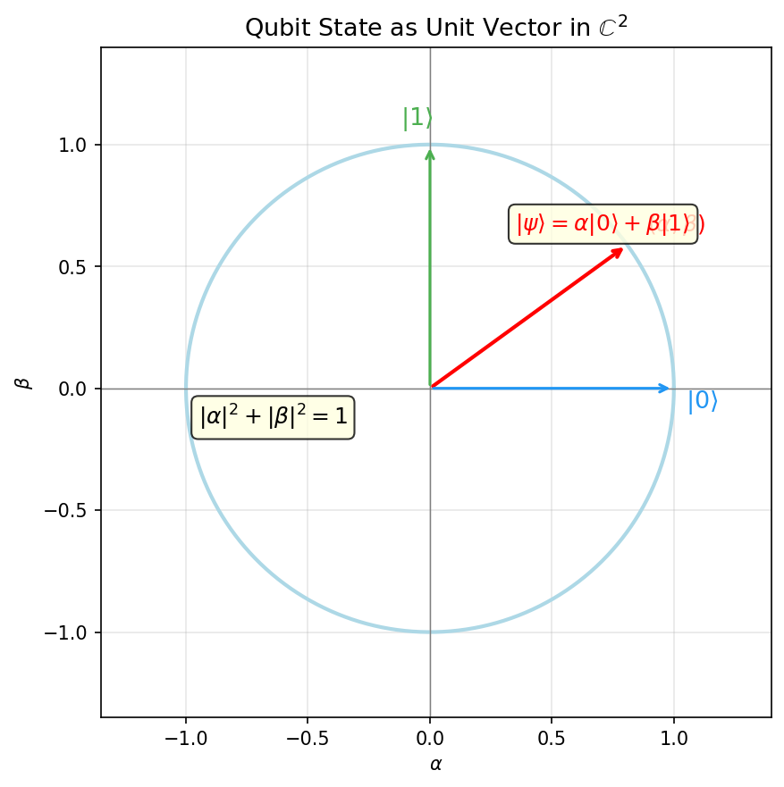
The qubit is the quantum analogue of the classical bit. Classically, a bit takes a definite value of 0 or 1. A qubit, by contrast, can exist in a continuous superposition of the two possibilities. Mathematically, the state of a qubit is a unit vector in the complex Hilbert space \(\mathbb{C}^2\).
Dirac’s bra-ket notation is the universal language for quantum mechanics. Its elegance lies in keeping track of the difference between a state vector and its dual, making inner products visually transparent.
Definition 1.1.1 (Ket). A quantum state vector is written in Dirac notation as \(|\psi\rangle \in \mathbb{C}^2\). This is called a ket.
The ket \(|\psi\rangle\) is simply a column vector in \(\mathbb{C}^2\), normalized to unit length. The name “ket” is the second half of “bracket” — its dual is the “bra” \(\langle\psi|\), and the inner product \(\langle\phi|\psi\rangle\) is a “bra-ket” or bracket.
The two standard basis states are the computational basis vectors:
\[|0\rangle = \begin{pmatrix}1\\0\end{pmatrix}, \qquad |1\rangle = \begin{pmatrix}0\\1\end{pmatrix}.\]A general single-qubit state is
\[|\psi\rangle = \alpha|0\rangle + \beta|1\rangle, \qquad \alpha,\beta \in \mathbb{C}, \quad |\alpha|^2 + |\beta|^2 = 1.\]The scalars \(\alpha\) and \(\beta\) are the probability amplitudes for outcomes \(|0\rangle\) and \(|1\rangle\), respectively. Unlike classical probabilities, amplitudes are complex numbers and can interfere constructively or destructively — a feature that quantum algorithms exploit.
Definition 1.1.2 (Probability Amplitude). Given a quantum state \(\alpha|0\rangle + \beta|1\rangle\), the coefficients \(\alpha, \beta \in \mathbb{C}\) are the probability amplitudes of \(|0\rangle\) and \(|1\rangle\) respectively.
The probability of observing outcome \(|0\rangle\) is \(|\alpha|^2\) and of \(|1\rangle\) is \(|\beta|^2\); normalization requires \(|\alpha|^2 + |\beta|^2 = 1\).
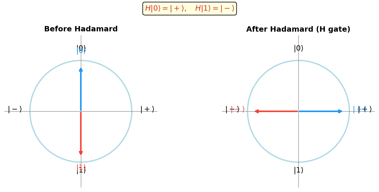
Important single-qubit states beyond the computational basis include the Hadamard basis states:
\[|{+}\rangle = \tfrac{1}{\sqrt{2}}(|0\rangle + |1\rangle), \qquad |{-}\rangle = \tfrac{1}{\sqrt{2}}(|0\rangle - |1\rangle).\]The concept of the dual vector completes the bra-ket framework, allowing inner products and measurement probabilities to be written compactly.
Definition 1.1.3 (Bra). The dual vector (conjugate transpose) of \(|\psi\rangle\) is \(\langle\psi|\). For \(|\psi\rangle = \alpha|0\rangle + \beta|1\rangle\), we have \(\langle\psi| = \bar\alpha\langle 0| + \bar\beta\langle 1|\).
The inner product of two states is written in bra-ket notation as \(\langle\phi|\psi\rangle\). For the computational basis: \(\langle 0|0\rangle = \langle 1|1\rangle = 1\) and \(\langle 0|1\rangle = 0\). The normalization condition \(\langle\psi|\psi\rangle = 1\) is the quantum analogue of requiring probabilities to sum to one — and both normalization conditions are mathematically equivalent to saying the state is a unit vector in the Hilbert space.
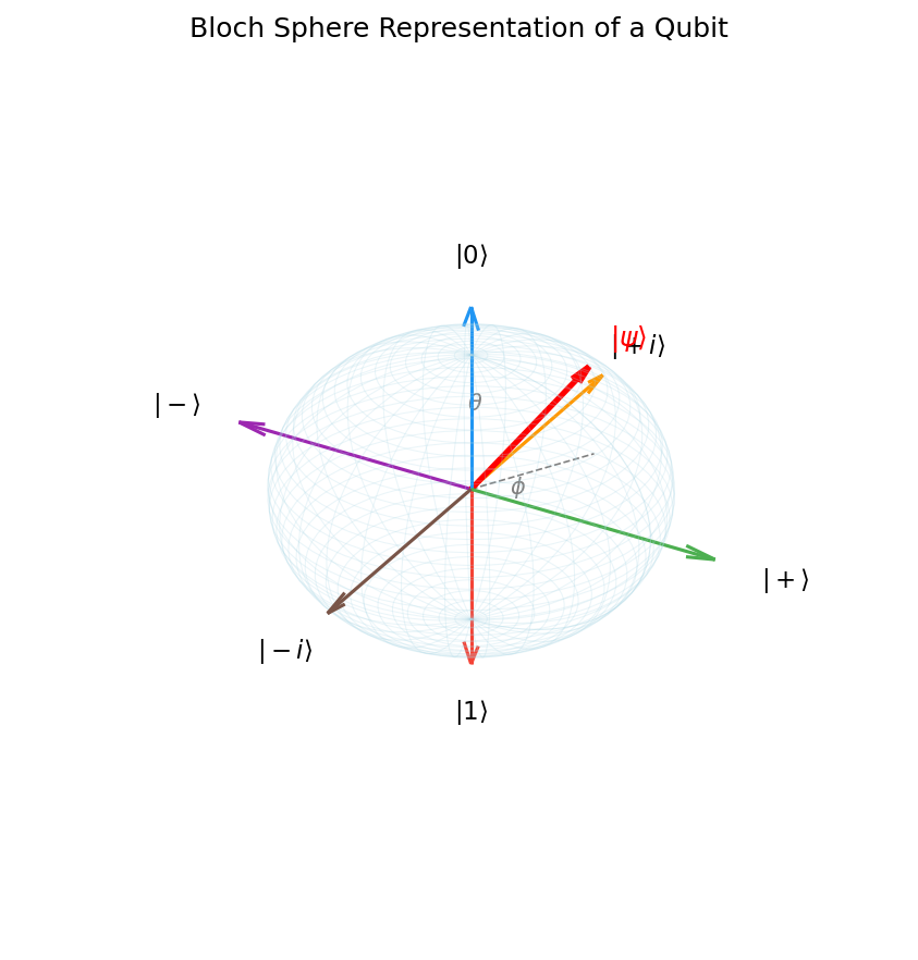
The Bloch Sphere. For a single qubit, the state space (up to a global phase) can be visualized as the surface of the unit sphere \(S^2\), called the Bloch sphere. Parameterizing by two real angles \(\theta \in [0,\pi]\) and \(\phi \in [0,2\pi)\),
\[|\psi\rangle = \cos\tfrac{\theta}{2}|0\rangle + e^{i\phi}\sin\tfrac{\theta}{2}|1\rangle.\]The north pole \((\theta = 0)\) is \(|0\rangle\), the south pole \((\theta = \pi)\) is \(|1\rangle\), and the equatorial states \((\theta = \pi/2)\) are superpositions. The Hadamard states \(|+\rangle\) and \(|-\rangle\) lie on opposite poles of the \(x\)-axis.
1.2 Projective Measurement and Bit Commitment
What happens when we look at a quantum system? Measurement is the bridge between the quantum world and classical observation. In quantum mechanics, measurement disturbs the system — after measuring, the state collapses to one of the eigenstates of the observable. This is fundamentally different from classical measurement, which we can imagine as passively reading out a pre-existing value.
After the measurement, the state collapses to \(|u_i\rangle\).
The probability formula \(p_i = |\langle u_i|\psi\rangle|^2\) is the Born rule — the fundamental link between the mathematical formalism and experimental outcomes. The squared modulus turns complex amplitudes into nonnegative probabilities, and the normalization \(\langle\psi|\psi\rangle = 1\) ensures they sum to one.
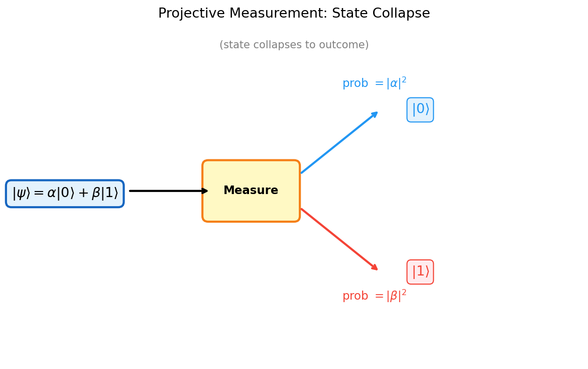
The collapse postulate is non-classical: measuring a state yields a random outcome and irreversibly changes the state. This is why quantum states cannot be copied (the no-cloning theorem) — measurement always disturbs the system.
A coarser notion is a projective measurement, specified by orthogonal projectors \(\{P_i\}_{i=1}^k\) with \(\sum_i P_i = I\). On state \(|\psi\rangle\):
Definition 1.4.2 (Projective Measurement). A projective measurement is specified by a sequence of orthogonal projection operators \(\{P_i : i \in [k]\}\) with \(\sum_{i=1}^k P_i = I\). On state \(|\psi\rangle \in \mathbb{C}^d\), outcome \(i\) occurs with probability \(\|P_i|\psi\rangle\|^2\), and the post-measurement state is \(P_i|\psi\rangle / \|P_i|\psi\rangle\|\).
General measurements are the most powerful. A general measurement of register \(M\) consists of preparing an ancilla register \(M'\) in the fixed state \(|\bar 0\rangle\), then performing a projective measurement on the composite system \(MM'\). This framework subsumes projective measurements as a special case.
Definition 1.4.3 (General Measurement). A general measurement of a register \(M\) with state space \(\mathbb{C}^{d_1}\) consists of preparing another register \(M'\) with state space \(\mathbb{C}^{d_2}\) in the fixed pure state \(|\bar{0}\rangle\), and measuring the composite system \(MM'\) according to a projective measurement on \(\mathbb{C}^{d_1} \otimes \mathbb{C}^{d_2}\).
Any other kind of measurement can be formulated as a general measurement, making this the most general framework for quantum measurement.
With a general measurement, the probability can be \(2/3\).
This illustrates why general measurements are strictly more powerful than projective measurements for state discrimination.
This means the probabilistic security of the quantum bit commitment protocol cannot be improved by using any more general measurement strategy.
1.3 Information Content of Quantum States
A striking fact about quantum mechanics is that despite the apparent richness of the qubit state — described by two continuous complex numbers — it cannot carry more classical information than a classical bit. This counterintuitive result is one of the most important theorems in quantum information theory.
The proof is dimension-theoretic: the \(2^m\) possible encoded states all lie in a subspace of dimension at most \(2^n\), and no measurement can perfectly distinguish more states than the dimension of the space. This is the quantum analogue of the classical source coding theorem — with the Hilbert space dimension playing the role of the codebook size.
This implies that \(n\) qubits can reliably encode at most \(n\) classical bits — there is no quantum advantage in terms of classical information capacity with a fixed distribution. This is related to the Holevo bound (Holevo 1973).
1.4 Quantum Bit Commitment
Bit commitment is a cryptographic primitive in which Alice commits to a bit \(a\) without revealing it, and later opens the commitment so Bob can verify. Classically, perfect bit commitment is impossible: either Bob can deduce \(a\) from the commitment (hiding fails), or Alice can later claim a different value (binding fails).
Quantum mechanics offers a near-solution. Let \(|\psi_0\rangle = \cos(\pi/8)|0\rangle + \sin(\pi/8)|1\rangle\) and \(|\psi_1\rangle = \sin(\pi/8)|0\rangle + \cos(\pi/8)|1\rangle\).
Commit: Alice prepares qubit M in state \(|\psi_a\rangle\) and sends M to Bob.
Reveal: Alice announces \(a\). Bob measures M in the basis \(\{|\psi_a\rangle, |\tilde\psi_a\rangle\}\) and accepts if the outcome is \(|\psi_a\rangle\).
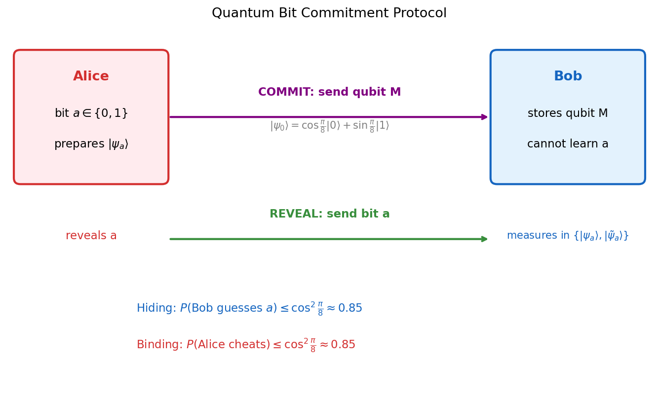
Proposition 1.2.1. The quantum bit commitment protocol satisfies the hiding and binding properties probabilistically:
- Hiding: \(\min_{a \in \{0,1\}} P(\text{Bob guesses } a) \leq \cos^2(\pi/8) \approx 0.85\), regardless of the measurement Bob makes.
- Binding: \(\min_{b \in \{0,1\}} P(\text{Bob accepts } b \mid \text{Alice cheats}) \leq \cos^2(\pi/8) \approx 0.85\).
While not perfectly secure (unlike classical impossibility, it provides probabilistic security with \(\delta \approx 0.85\)), this demonstrates a genuine quantum advantage. Importantly, even the most general quantum strategy for Alice cannot improve the cheating probability beyond \(\cos^2(\pi/8)\).
This shows the binding property of the quantum protocol holds against any quantum adversary, not just those restricted to pure states.
Chapter 2: Multiple Qubits and Entanglement
When we combine multiple quantum systems, the resulting state space is dramatically larger than the sum of its parts. Chapter 2 introduces the tensor product formalism for multi-qubit systems and the phenomenon of entanglement — quantum correlations that have no classical analogue and underlie the most powerful quantum protocols.
2.1 Multi-Qubit States and Tensor Products
The state space of \(n\) qubits is not \(n\) copies of \(\mathbb{C}^2\) laid side by side — it is their tensor product: a \(2^n\)-dimensional Hilbert space \((\mathbb{C}^2)^{\otimes n}\). This exponential scaling is both the source of quantum computational power and the fundamental obstacle to simulating quantum systems classically.
where \(d = 2^n\).
The \(2^n\) amplitudes \(\{\alpha_x\}_{x \in \{0,1\}^n}\) are complex numbers whose squared moduli are probabilities. Storing and manipulating this vector classically requires exponential resources — which is why quantum computers, which naturally manipulate such states, may offer exponential advantages.
The tensor product is bilinear and captures the idea of independent quantum systems: if system \(A\) is in state \(|u\rangle\) and system \(B\) is in state \(|v\rangle\), their joint state is \(|u\rangle \otimes |v\rangle\). Not all states in \(\mathbb{C}^{d_1} \otimes \mathbb{C}^{d_2}\) are of this product form — the ones that are not are entangled.
Proposition 1.3.2. The tensor product operation is bilinear:
- For all \(\alpha \in \mathbb{C}\), \(|u\rangle \in \mathbb{C}^{d_1}\), \(|v\rangle \in \mathbb{C}^{d_2}\): \((\alpha|u\rangle) \otimes |v\rangle = \alpha(|u\rangle \otimes |v\rangle) = |u\rangle \otimes (\alpha|v\rangle)\).
- For all \(|u_1\rangle, |u_2\rangle \in \mathbb{C}^{d_1}\), \(|v\rangle \in \mathbb{C}^{d_2}\): \((|u_1\rangle + |u_2\rangle) \otimes |v\rangle = |u_1\rangle \otimes |v\rangle + |u_2\rangle \otimes |v\rangle\).
- For all \(|u\rangle \in \mathbb{C}^{d_1}\), \(|v_1\rangle, |v_2\rangle \in \mathbb{C}^{d_2}\): \(|u\rangle \otimes (|v_1\rangle + |v_2\rangle) = |u\rangle \otimes |v_1\rangle + |u\rangle \otimes |v_2\rangle\).
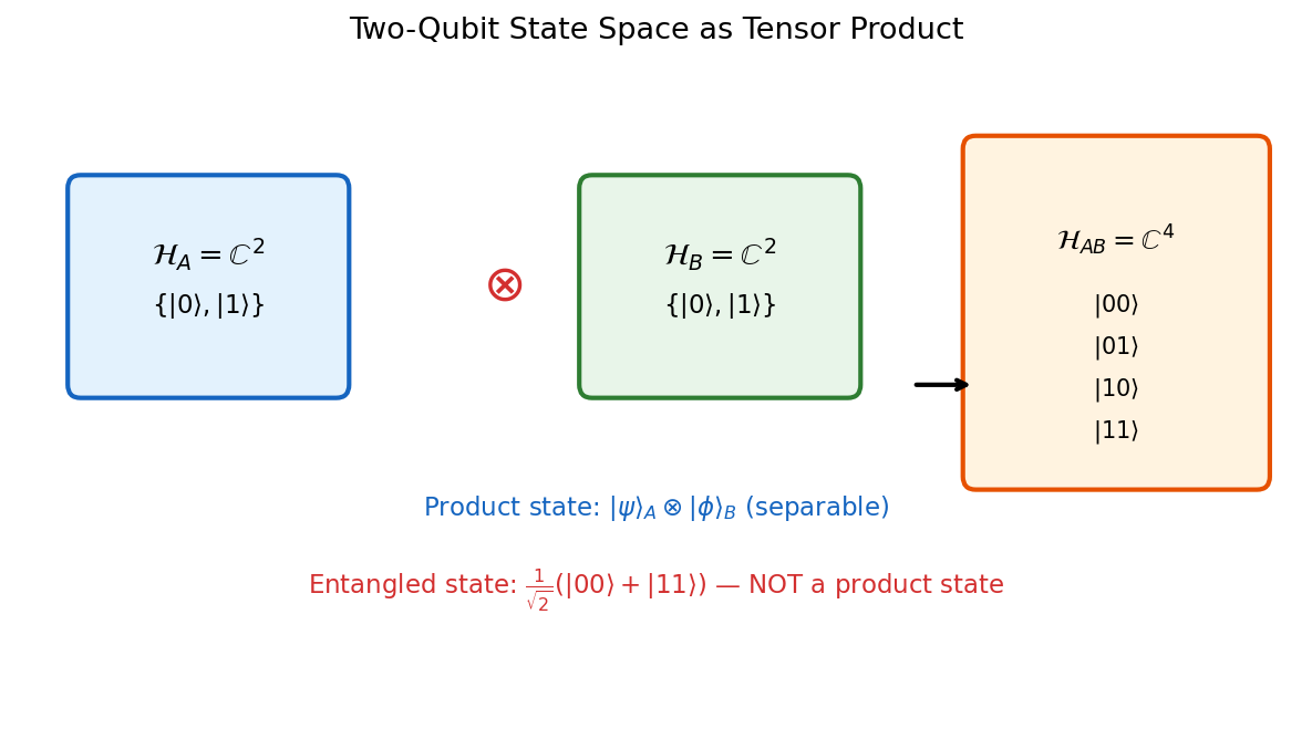
The tensor product is bilinear. Crucially, not every vector in \(\mathbb{C}^{d_1} \otimes \mathbb{C}^{d_2}\) is a product state.
The distinction between product states and entangled states is the most important conceptual divide in quantum information theory.
Definition 1.3.3 (Product State). Vectors which may be written as the tensor product of two vectors are product states. The rest — those unable to be written this way — are entangled states.
The state \(\frac{1}{\sqrt{2}}(|01\rangle + |10\rangle)\) cannot be written as \(|u\rangle \otimes |v\rangle\) for any single-qubit states — this is entanglement. Entanglement is a purely quantum phenomenon with no classical analogue: the two qubits exhibit correlations that are stronger than any classical correlations, even when the qubits are spatially separated. The Bell inequalities make this formal: no local hidden variable theory can reproduce the correlations of an entangled pair.
Bell’s Inequality and Nonlocality
Entanglement is not merely a mathematical curiosity — it has physical consequences that sharply distinguish quantum mechanics from any classical theory. The question of whether quantum correlations can be explained by classical means was posed precisely by John Bell in 1964 and refined into a testable inequality by Clauser, Horne, Shimony, and Holt (CHSH) in 1969. Their work answers a foundational question: can the outcomes of quantum measurements be explained by pre-determined “hidden variables” that each particle carries with it?
A hidden variable theory posits that every physical system has a definite, pre-existing value for every possible measurement, and that the apparent randomness of quantum mechanics arises only from our ignorance of these values. Bell’s profound insight was that such theories impose quantitative constraints on the correlations between measurements on separate systems — constraints that quantum mechanics violates.
Since \(B_0, B_1 \in \{-1, +1\}\), exactly one of \(B_0 + B_1\) and \(B_0 - B_1\) is zero and the other is \(\pm 2\). Therefore the entire expression has absolute value at most \(2\). \(\square\)
The CHSH inequality has an elegant reformulation in the language of computer science. Consider a cooperative game played by Alice and Bob: a referee samples bits \(s, t \in \{0,1\}\) uniformly at random and sends \(s\) to Alice and \(t\) to Bob. Without communicating, Alice outputs a bit \(a\) and Bob outputs a bit \(b\). They win if and only if \(a \oplus b = s \cdot t\). This is called the CHSH game. When \(s \cdot t = 0\) (three of the four input pairs), they need to agree; when \(s \cdot t = 1\), they need to disagree.
Theorem 2.1.4 (Classical Bound for the CHSH Game). For any classical strategy (including shared randomness but no communication), the maximum winning probability in the CHSH game is \(\frac{3}{4}\).
The surprise is that quantum entanglement breaks this barrier. Suppose Alice and Bob share the Bell state \(\frac{1}{\sqrt{2}}(|00\rangle - |11\rangle)\). Upon receiving \(s\), Alice rotates her qubit by angle \(\frac{\pi}{16}\) when \(s = 0\) and by \(\frac{3\pi}{16}\) when \(s = 1\), then measures; Bob applies a rotation by \(\frac{\pi}{16}\) when \(t = 0\) and by \(-\frac{3\pi}{16}\) when \(t = 1\), then measures. For each input pair, the probability of satisfying \(a \oplus b = s \cdot t\) is exactly \(\cos^2(\pi/8)\).
which exceeds the classical bound of \(\frac{3}{4}\).
The quantum winning probability corresponds, via the CHSH expression, to a value of \(2\sqrt{2} \approx 2.83\), violating the classical bound of \(2\). A natural question is whether even stronger quantum strategies exist.
Tsirelson’s bound shows that quantum mechanics is strictly stronger than classical mechanics for this task, but not maximally so — a hypothetical theory could in principle achieve a winning probability of \(1\) without communication. That quantum mechanics saturates the bound at \(2\sqrt{2}\) rather than \(4\) is a deep fact whose full information-theoretic explanation remains an active area of research.
In 1982, Alain Aspect and collaborators carried out the first convincing experimental test of Bell’s inequality, confirming the quantum prediction and ruling out local hidden variable theories. Subsequent experiments with ever-tightening loopholes have reaffirmed this conclusion: nature is nonlocal in the precise sense that entangled particles exhibit correlations that no classical theory respecting locality can reproduce. From the perspective of computer science, nonlocality means that entanglement is a genuine computational resource — it enables cooperative tasks that are provably impossible classically without communication.
2.2 The Bell States
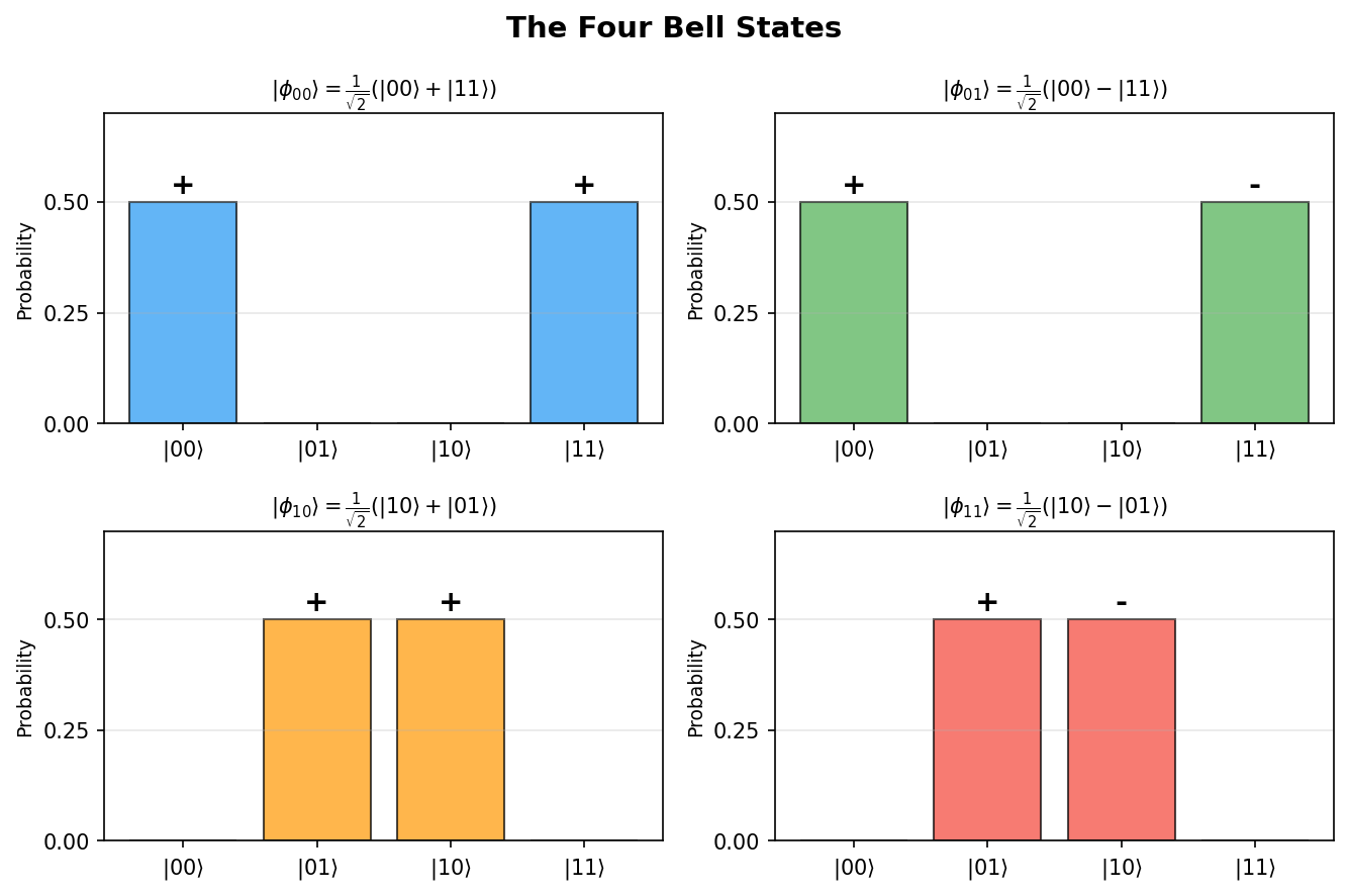
Among all two-qubit states, the Bell states are the maximally entangled ones — they are the canonical resource for quantum communication protocols like superdense coding and teleportation. Every quantum information student should know these four states by heart.
The four Bell states (also called EPR pairs) are the maximally entangled two-qubit states:
\[|\phi_{00}\rangle = \tfrac{1}{\sqrt{2}}(|00\rangle + |11\rangle), \qquad |\phi_{01}\rangle = \tfrac{1}{\sqrt{2}}(|00\rangle - |11\rangle),\]\[|\phi_{10}\rangle = \tfrac{1}{\sqrt{2}}(|10\rangle + |01\rangle), \qquad |\phi_{11}\rangle = \tfrac{1}{\sqrt{2}}(|10\rangle - |01\rangle).\]These four states form an orthonormal basis of \(\mathbb{C}^2 \otimes \mathbb{C}^2\), called the Bell basis. A key identity is
\[|\phi_{ab}\rangle = (X^a Z^b \otimes I)|\phi_{00}\rangle,\]which says that all four Bell states can be obtained from a single EPR pair by applying Pauli operators to one qubit.
2.3 Measuring a Subsystem
When we measure only part of a composite system, the measurement on the subsystem \(A\) of \(AB\) is equivalent to measuring the entire system according to the operators \(\{P_i \otimes I_B\}\).
By the Schmidt decomposition theorem, any state \(|\psi\rangle \in \mathbb{C}^{d_1} \otimes \mathbb{C}^{d_2}\) can be written as
\[|\psi\rangle = \sum_{i=1}^{d_1} \alpha_i |u_i\rangle_A |v_i\rangle_B,\]where \(\{|u_i\rangle\}\), \(\{|v_i\rangle\}\) are orthonormal sets and \(\alpha_i \geq 0\). Measuring register \(A\) in the basis \(\{|u_i\rangle\}\) yields outcome \(i\) with probability \(|\alpha_i|^2\), leaving the system in the product state \(|u_i\rangle_A |v_i\rangle_B\). This is how entanglement is broken by measurement.
2.4 Tensor Products of Operators
If \(U\) acts on system \(A\) and \(V\) acts on system \(B\), the joint operator on \(AB\) is \(U \otimes V\), defined on product states by
\[(U \otimes V)(|u\rangle \otimes |v\rangle) = U|u\rangle \otimes V|v\rangle.\]and extended by linearity.
Key properties include \((U_1 \otimes V_1)(U_2 \otimes V_2) = (U_1 U_2) \otimes (V_1 V_2)\), \((U \otimes V)^\dagger = U^\dagger \otimes V^\dagger\), \((U \otimes V)^{-1} = U^{-1} \otimes V^{-1}\), and \(\|U \otimes V\| = \|U\| \cdot \|V\|\). When only subsystem \(A\) evolves by \(U\), the full evolution is \(U \otimes I_B\).
The outer product is the fundamental building block for writing operators in terms of basis vectors: any operator \(U = (\alpha_{ij})\) can be expressed as \(U = \sum_{i,j} \alpha_{ij} |e_i\rangle\langle e_j|\).
2.5 Density Matrices and the Partial Trace
So far, every quantum state we have considered has been a pure state — a unit vector \(|\psi\rangle\) in some Hilbert space. Pure states suffice when we have complete knowledge of a quantum system in isolation. But when we measure only part of a composite system, or when a system is prepared by a random process, the resulting state of the subsystem is in general not a pure state. To describe such situations, we need a more general formalism: density matrices.
Observables and Expected Values
Before introducing density matrices, we formalize the notion of a quantum observable. In quantum mechanics, every measurable physical quantity corresponds to a Hermitian operator.
where \(a_j \in \mathbb{R}\) are the distinct eigenvalues and \(P_j\) are the projections onto the corresponding eigenspaces, with \(\sum_j P_j = I\).
Example 2.5.1. The Pauli \(Z\) operator has spectral decomposition \(Z = (+1)|0\rangle\langle 0| + (-1)|1\rangle\langle 1|\). Measuring \(Z\) on \(|\psi\rangle = \alpha|0\rangle + \beta|1\rangle\) yields \(+1\) with probability \(|\alpha|^2\) and \(-1\) with probability \(|\beta|^2\). The projector \(P_1 = |1\rangle\langle 1|\) is also a valid observable, with eigenvalues \(0\) and \(1\); measuring \(P_1\) gives the same outcome probabilities as a computational basis measurement, but the eigenvalues are \(0, 1\) instead of \(+1, -1\).
The Density Matrix
The need for density matrices arises naturally from the study of composite systems. Suppose Alice and Bob share the Bell state \(\frac{1}{\sqrt{2}}(|00\rangle + |11\rangle)\). If we ask “what is the state of Alice’s qubit alone?”, the answer cannot be any pure state — Alice’s qubit is equally likely to be found in \(|0\rangle\) or \(|1\rangle\), but it is not in the superposition \(\frac{1}{\sqrt{2}}(|0\rangle + |1\rangle)\), because that state has definite measurement outcomes in the \(|+\rangle, |-\rangle\) basis, whereas Alice’s qubit is maximally uncertain in every basis. The correct description is a mixed state, represented by a density matrix.
Definition 2.5.2 (Density Matrix). A density matrix (or density operator) on \(\mathbb{C}^d\) is a positive semidefinite operator \(\rho\) with \(\operatorname{Tr}(\rho) = 1\).
- A pure state \(|\psi\rangle\) corresponds to the density matrix \(\rho = |\psi\rangle\langle\psi|\).
- A mixed state described by the ensemble \(\{(p_i, |\psi_i\rangle)\}\) — meaning state \(|\psi_i\rangle\) occurs with classical probability \(p_i\) — corresponds to the density matrix \(\rho = \sum_i p_i |\psi_i\rangle\langle\psi_i|\).
The key properties of density matrices mirror and generalize the pure-state formalism:
Proposition 2.5.1. Let \(\rho\) be a density matrix on \(\mathbb{C}^d\). Then:
- \(\rho \geq 0\) (positive semidefinite) and \(\operatorname{Tr}(\rho) = 1\).
- The probability that a projective measurement \(\{\Pi_j\}\) yields outcome \(j\) is \(\operatorname{Tr}(\Pi_j \rho)\).
- The expected value of an observable \(M\) is \(\langle M \rangle = \operatorname{Tr}(M\rho)\). For a pure state \(\rho = |\psi\rangle\langle\psi|\), this reduces to \(\langle\psi|M|\psi\rangle\).
- Under unitary evolution \(U\), the density matrix transforms as \(\rho \mapsto U\rho U^\dagger\).
A crucial conceptual point is that a given density matrix may admit multiple ensemble decompositions, and these are physically indistinguishable.
and indeed as \(\frac{1}{2}|u\rangle\langle u| + \frac{1}{2}|u^\perp\rangle\langle u^\perp|\) for any orthonormal basis \(\{|u\rangle, |u^\perp\rangle\}\). No measurement can distinguish these preparations.
Since \(\rho\) is Hermitian and positive semidefinite, it admits a spectral decomposition \(\rho = \sum_j \lambda_j |e_j\rangle\langle e_j|\) where \(\lambda_j \geq 0\), \(\sum_j \lambda_j = 1\), and \(\{|e_j\rangle\}\) are orthonormal eigenvectors. A state is pure if and only if \(\rho^2 = \rho\), equivalently if and only if \(\operatorname{Tr}(\rho^2) = 1\). For mixed states, \(\operatorname{Tr}(\rho^2) < 1\), and this quantity — called the purity — measures how far the state is from being pure.
The Partial Trace
The partial trace is the mathematical operation that extracts the local description of a subsystem from the global state of a composite system.
and extended by linearity. The reduced density matrix of the first system is \(\rho_1 = \operatorname{Tr}_2(\rho)\).
In concrete matrix terms, if \(\rho\) is written in block form with \(d_2 \times d_2\) blocks \(B_{ik}\), then the \((i,k)\)-entry of \(\operatorname{Tr}_2(\rho)\) is \(\operatorname{Tr}(B_{ik})\).
Alice’s qubit is in the maximally mixed state — she has no local information about the entangled pair.
The partial trace has a fundamental operational property: local operations on one subsystem cannot affect the reduced density matrix of the other.
Anything Bob does to his subsystem leaves Alice’s reduced density matrix unchanged. This is the no-signaling principle: entanglement alone cannot transmit information.
Purification
The relationship between pure and mixed states is made precise by the concept of purification: every mixed state arises as the reduced state of some pure state in a larger system.
Theorem 2.5.4 (Purification). For any density matrix \(\rho\) on \(\mathbb{C}^{d_1}\), there exists a pure state \(|\psi\rangle \in \mathbb{C}^{d_1} \otimes \mathbb{C}^{d_2}\) (with \(d_2 \geq \operatorname{rank}(\rho)\)) such that \(\operatorname{Tr}_2(|\psi\rangle\langle\psi|) = \rho\).
Purifications are not unique, but any two purifications of the same density matrix in the same dimension are related by a local unitary on the purifying system.
Proposition 2.5.5. If \(|\psi\rangle\) and \(|\phi\rangle\) are both purifications of \(\rho\) in \(\mathbb{C}^{d_1} \otimes \mathbb{C}^{d_2}\), then there exists a unitary \(U\) on \(\mathbb{C}^{d_2}\) such that \(|\phi\rangle = (I \otimes U)|\psi\rangle\).
This result, combined with the no-signaling principle, yields the impossibility of quantum bit commitment: if a commitment protocol is perfectly hiding (Bob’s reduced state is the same for both committed values), then Alice’s global states for the two commitments are purifications of the same density matrix. By Proposition 2.5.5, a local unitary on Alice’s register converts one to the other — so Alice can cheat by switching her commitment after the commit phase, an operation Bob cannot detect.
Chapter 3: Quantum Gates and Circuits
Armed with the formalism of quantum states and measurement, we now ask: how do we process quantum information? Chapter 3 develops the quantum circuit model — the quantum analogue of the Boolean circuit model — and establishes universality results showing that a small set of quantum gates suffices for all quantum computation.
3.1 Classical and Quantum Computation Models
To understand quantum computation, it helps to first recall the classical model precisely. A classical circuit consists of memory bits and logic gates. The time complexity is the number of gates, and the space complexity is the number of bits. A gate set is universal if any boolean function can be computed using it; \(\{\text{NOT}, \text{AND}\}\) suffices.
Theorem 3.1.1. Any function \(f : \{0,1\}^n \to \{0,1\}^m\) can be computed by a Boolean circuit over the gate set \(\{\text{NOT}, \text{AND}\}\).
Definition 3.1.1 (Universal). A set of gates \(G\) is universal if any function \(\{0,1\}^n \to \{0,1\}^m\) can be computed by a Boolean circuit over \(G\).
Definition 3.1.2 (Efficient). A circuit/algorithm is efficient if its time complexity is \(O(n^k)\) for some constant \(k\), where \(n\) denotes the number of input bits.
for all inputs \(x\).
A randomized circuit initializes some memory bits to uniformly random values, giving a distribution over outputs. It computes \(f\) if the probability of a correct output exceeds \(2/3\). The quantum model generalizes this by replacing bits with qubits, random initialization with prepared quantum states, and probabilistic gates with unitary transformations.
3.2 Quantum Gates and Circuits
The quantum circuit model is the standard model for quantum computation. It closely parallels the classical circuit model, with qubits replacing bits and unitary matrices replacing Boolean gates.
Definition 3.2.1 (Quantum Circuit). A quantum circuit consists of:
- The memory, consisting of qubits.
- Quantum gates, which perform unitary operations on a small constant number of qubits.
- Measurements in the standard (Z) basis.
The restriction to unitary gates on a constant number of qubits at a time reflects a physical constraint: we can only apply local interactions. The requirement for unitarity (as opposed to arbitrary linear maps) is the mathematical expression of the physical law that quantum evolution is reversible.
Because quantum evolution must be reversible (unitary), quantum gates are invertible. The evolution of a closed quantum system is linear, reversible, and norm-preserving — hence described by a unitary operator.
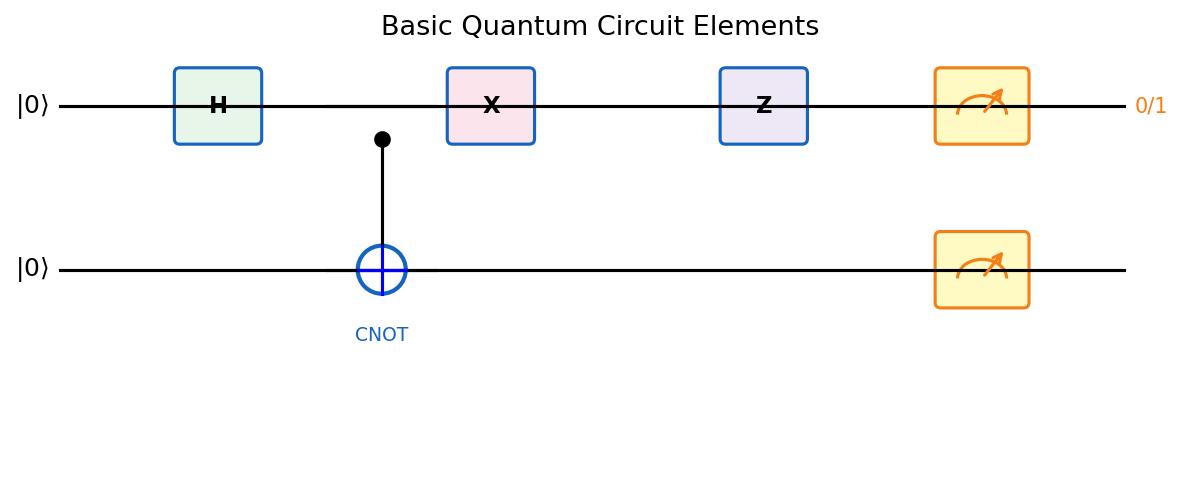
Key single-qubit gates include:
- Hadamard gate: \(H = \frac{1}{\sqrt{2}}\begin{pmatrix}1&1\\1&-1\end{pmatrix}\), maps \(|0\rangle \mapsto |{+}\rangle\), \(|1\rangle \mapsto |{-}\rangle\).
- Pauli X (NOT): \(X = \begin{pmatrix}0&1\\1&0\end{pmatrix}\), flips \(|0\rangle \leftrightarrow |1\rangle\).
- Pauli Z (phase flip): \(Z = \begin{pmatrix}1&0\\0&-1\end{pmatrix}\), maps \(|+\rangle \leftrightarrow |-\rangle\).
- Pauli Y: \(Y = \begin{pmatrix}0&-i\\i&0\end{pmatrix} = iXZ\).
- T gate: \(T = \begin{pmatrix}1&0\\0&e^{i\pi/4}\end{pmatrix}\), a \(\pi/4\) phase rotation.
The Hadamard gate is especially important: applied to a computational basis state, it creates an equal superposition over all values, enabling quantum parallelism.
The CNOT gate (controlled-NOT) is the canonical two-qubit gate:
\[\text{CNOT}: |a\rangle|b\rangle \mapsto |a\rangle|b \oplus a\rangle.\]It flips the target qubit if and only if the control qubit is \(|1\rangle\). The CNOT, combined with single-qubit gates, is universal for quantum computation.
The Toffoli gate is a 3-qubit gate: \(|a\rangle|b\rangle|c\rangle \mapsto |a\rangle|b\rangle|c \oplus (a \cdot b)\rangle\). It is a controlled-controlled-NOT. With ancillas initialized to \(|0\rangle\) and \(|1\rangle\), the Toffoli gate can simulate both AND and NOT gates, giving universal classical computation.
3.3 Universality of Quantum Gate Sets
Just as classical computation can be realized with a small finite gate set (e.g., NAND), quantum computation can be realized with a small finite gate set. The universality theorems justify why we need only a handful of standard gates in all quantum algorithms.
Theorem 3.3.1. For any unitary operation \(U\) on \(\mathbb{C}^d\), \(d = 2^n\), there is a quantum circuit using only CNOT gates and single-qubit gates that computes \(U\). Hence \(\{\text{CNOT}\} \cup U(2)\) is a universal gate set.
Definition 3.3.1 (Universal Gate Set, exact version). A gate set \(G\) is universal if for any unitary operation \(U\) on \(\mathbb{C}^d\), \(d = 2^n\), there is a quantum circuit using only gates from \(G\) that computes \(U\).
This tells us that all quantum computation reduces to two-qubit interactions (CNOT) and single-qubit rotations. The infinite gate set \(U(2)\) is not physically implementable, but it can be approximated with a finite set — and the approximation error is quantitatively controlled by the Solovay-Kitaev theorem.
For practical purposes, we want a finite gate set. Approximation is the key concept:
Definition 3.3.2 (Operator Approximation). We say that a unitary operator \(V\) on \(\mathbb{C}^d\), \(d = 2^n\), approximates another, \(U\), with error \(\varepsilon \in (0,1)\) if \(\|U - V\| \leq \varepsilon\).
Definition 3.3.3 (Circuit Approximation). We say a quantum circuit approximates a unitary operator \(U\) with error \(\varepsilon \in (0,1)\) if it computes a unitary operator \(V\) such that \(\|U - V\| \leq \varepsilon\).
Definition 3.3.4 (Universal Gate Set, approximate version). Let \(G\) be a gate set. We say \(G\) is universal if for any unitary operation \(U\) on \(\mathbb{C}^d\), \(d = 2^n\), and any \(\varepsilon \in (0,1)\), there is a quantum circuit using only gates from \(G\) computing \(V\) with \(\|U - V\| \leq \varepsilon\).
Theorem 3.3.4. The gate set \(\{CNOT, H, T\}\) is universal.
The surprising fact that just three gates — CNOT, Hadamard, and the T gate — suffice for all quantum computation is the quantum analogue of the universality of NAND in classical computation.
Theorem 3.3.6 (Solovay-Kitaev). For any \(\varepsilon \in (0,1)\) and \(U \in U(2)\), there exists a sequence of \(O(\log^c(1/\varepsilon))\) gates from \(\{H,T\}\) that approximates \(U\) to within \(\varepsilon\), where \(c\) is a universal constant close to 2.
If each gate in a circuit of size \(m\) is approximated with error \(\varepsilon/m\), the entire circuit has error at most \(\varepsilon\) — this is the key composability result for approximate circuits.
In particular, if each \(\varepsilon_i = \varepsilon/t\), the composed circuits have total error at most \(\varepsilon\).
3.4 Implementing Measurements and Complexity Classes
The quantum circuit model handles measurements by a simple basis-change trick: any projective measurement can be reduced to a standard-basis measurement.
Any projective measurement can be implemented by:
- Applying a basis-change unitary \(U\) so that the measurement basis becomes the computational basis.
- Measuring in the standard basis.
- Applying \(U^\dagger\) to restore the original basis.
For quantum algorithms, the relevant complexity classes are:
Definition 3.5.1 (Polynomial Time). The complexity class \(\mathbf{P}\) consists of all families of Boolean functions \(\{f_n : \{0,1\}^n \to \{0,1\}\}\) which have efficient deterministic classical circuits.
\(\mathbf{P}\) is the class of problems a deterministic computer can solve efficiently. It is worth understanding the hierarchy of these three classes — P, BPP, BQP — as three increasingly powerful computational models, each obtained by broadening the resources available. P allows only deterministic computation. BPP adds the ability to flip coins. BQP adds the ability to manipulate quantum superpositions and interference.
Definition 3.5.2 (Bounded-Error Probabilistic Polynomial Time). The complexity class \(\mathbf{BPP}\) consists of all families of Boolean functions \(\{f_n : \{0,1\}^n \to \{0,1\}\}\) which have efficient randomized classical circuits (success probability at least \(2/3\)).
Notice that the error threshold \(2/3\) in the BPP definition is a convention, not a hard boundary. Any constant success probability strictly above \(1/2\) defines the same class — by running the algorithm \(O(\log(1/\delta))\) times and taking the majority vote, the error can be reduced to any desired \(\delta\) while increasing the running time by only a logarithmic factor. This amplification trick applies equally to BQP. In practice, BPP contains many problems of practical importance: primality testing (before Agrawal-Kayal-Saxena, and still used in fast cryptographic practice), polynomial identity testing, approximate counting, and most optimization heuristics.
Definition 3.5.3 (Bounded-Error Quantum Polynomial Time). The complexity class \(\mathbf{BQP}\) consists of all families of Boolean functions \(\{f_n : \{0,1\}^n \to \{0,1\}\}\) which have efficient quantum circuits (success probability at least \(2/3\)).
BQP is the quantum analogue of BPP. The threshold \(2/3\) is conventional but not critical: by repeating and majority-voting, any constant success probability above \(1/2\) can be boosted to exponentially close to 1 using polynomially many repetitions.
Before stating the containment theorems, let us pause to think about what they ought to say. We have built an entirely new model of computation — qubits, unitaries, interference — and it would be alarming if this model could not reproduce what a classical computer does. Classical deterministic computation is just a degenerate special case of quantum computation (use only computational basis states and permutation matrices), so \(P \subseteq BQP\) is conceptually immediate. The more interesting question is whether a quantum computer can also simulate a classical randomized algorithm — one that uses random coin flips. The answer is yes, but the argument requires a moment’s care: we must simulate coin flips with Hadamard gates and then uncompute the randomness so the ancilla qubits are returned to \(|0\rangle\), avoiding unwanted entanglement between the random register and the computation register.
Theorem 3.5.1. The complexity classes \(\mathbf{P}\) and \(\mathbf{BQP}\) satisfy \(P \subseteq BQP\).
Theorem 3.5.2. The complexity classes \(\mathbf{BPP}\) and \(\mathbf{BQP}\) satisfy \(BPP \subseteq BQP\).
The chain \(P \subseteq BPP \subseteq BQP\) establishes that quantum computers are at least as powerful as classical ones. But the deeper and more exciting question is whether the containment \(BPP \subsetneq BQP\) is strict — that is, whether quantum computers can solve problems that are intractable for any classical probabilistic algorithm. The consensus answer is yes: Shor’s algorithm gives the strongest evidence, since factoring is widely believed not to be in BPP. Yet no formal proof of \(BPP \neq BQP\) exists; proving it would require proving \(P \neq PSPACE\), which remains one of the great open problems in complexity theory. What we can say is that the evidence strongly favors strict containment — and that the power of quantum computation arises precisely from interference effects that have no classical probabilistic analogue.
The relations \(P \subseteq BPP \subseteq BQP\) hold, meaning quantum computers can efficiently simulate both deterministic and randomized classical computation. Simulating a classical circuit \(U_f : |x,\bar 0,\bar 0\rangle \mapsto |x, f(x), \bar 0\rangle\) quantumly requires a “compute-copy-uncompute” procedure to clean up ancilla qubits, using at most \(s + 2t + m\) qubits and \(O(t)\) quantum gates for a circuit of space \(s\) and time \(t\).
The “compute-copy-uncompute” structure deserves emphasis because it illustrates a fundamental principle of quantum computation: ancilla qubits must be returned to a fixed state (usually \(|0\rangle\)) before they are discarded. If they are simply thrown away while entangled with the computation, their entanglement with the output register causes decoherence — the quantum state of the output becomes mixed, losing the superposition needed for interference. This is why quantum circuits require careful bookkeeping of all intermediate state, and it is one of the central challenges in designing efficient quantum algorithms: every intermediate classical bit must ultimately be “uncomputed” or stored in a separate register.
NP and Certificate-Based Computation
We now broaden our view of computational complexity to include nondeterministic classes, quantum analogues, and interactive proof systems.
The string \(y\) is called a certificate (or witness) for \(x\).
Intuitively, NP is the class of problems for which a “yes” answer can be efficiently verified, even if finding the answer may be hard. For example, a valid 3-colouring of a graph is a certificate for membership in 3-COLOURABLE: given the colouring, one can check in polynomial time that every edge connects vertices of different colours.
Definition 3.5.5 (Polynomial-time reduction). A language \(L_1\) is polynomial-time reducible to \(L_2\), written \(L_1 \leq_p L_2\), if there exists a polynomial-time computable function \(R\) such that \(x \in L_1 \iff R(x) \in L_2\).
Definition 3.5.6 (NP-completeness). A language \(L\) is NP-hard if every language in NP is polynomial-time reducible to \(L\). It is NP-complete if, additionally, \(L \in \text{NP}\).
NP-complete problems are the “hardest” problems in NP: solving any one of them in polynomial time would imply \(\text{P} = \text{NP}\).
Theorem 3.5.7 (Cook–Levin). CIRCUIT_SAT is NP-complete.
From this single result, a rich web of reductions establishes NP-completeness for SAT, 3-SAT, 3-COLOURING, TRAVELLING SALESMAN, SUBSET SUM, and many others. Not every problem in NP is believed to be either in P or NP-complete. Several important problems — graph automorphism, integer factoring, the discrete logarithm — are conjectured to inhabit the intermediate region. Factoring is particularly significant: Shor’s algorithm places it in BQP, yet no efficient classical algorithm is known.
QMA: Quantum Certificates
Definition 3.5.8 (QMA — Quantum Merlin-Arthur). A language \(L\) is in QMA if there exists a quantum polynomial-time verifier \(V\) and a polynomial \(p\) such that:
- Completeness: if \(x \in L\), there exists a \(p(|x|)\)-qubit quantum state \(|\psi\rangle\) with \(\Pr[V(x, |\psi\rangle) \text{ accepts}] \geq \frac{2}{3}\).
- Soundness: if \(x \notin L\), then for all \(p(|x|)\)-qubit states \(|\psi\rangle\), \(\Pr[V(x, |\psi\rangle) \text{ accepts}] \leq \frac{1}{3}\).
QMA is the quantum analogue of NP: a computationally unbounded prover prepares a quantum proof state, and a polynomial-time quantum verifier checks it. The \(k\)-local Hamiltonian problem — given \(H = \sum_i H_i\) where each \(H_i\) acts on at most \(k\) qubits, decide whether the ground state energy is below \(a\) or above \(b\) — is QMA-complete (Kitaev), the quantum analogue of the Cook-Levin theorem.
Interactive Proof Systems
Theorem 3.5.9 (Shamir, 1992). \(\mathrm{IP} = \mathrm{PSPACE}\).
Theorem 3.5.10 (Jain, Ji, Upadhyay, Watrous, 2011). \(\mathrm{QIP} = \mathrm{PSPACE}\).
All the containments \(\text{P} \subseteq \text{BPP} \subseteq \text{BQP}\) and \(\text{P} \subseteq \text{NP}\) are believed strict. The relationship between NP and BQP remains open: neither \(\text{NP} \subseteq \text{BQP}\) nor \(\text{BQP} \subseteq \text{NP}\) is known.
Chapter 4: Quantum Protocols
With the quantum circuit model established, Chapter 4 applies the theory to concrete protocols. Superdense coding and teleportation reveal how entanglement and quantum channels can be combined to achieve communication feats impossible classically. QKD shows that quantum mechanics provides unconditional security for key distribution — a guarantee impossible with any classical system.
4.1 Superdense Coding
Superdense coding is a striking protocol in which Alice transmits two classical bits to Bob by sending only one qubit — provided they share an entangled pair. At first glance, this seems to violate Holevo’s theorem, but the resolution is that the pre-shared entanglement is a non-trivial resource that augments the classical capacity of the quantum channel.
The protocol uses the key algebraic identity \(|\phi_{ab}\rangle = (X^a Z^b \otimes I)|\phi_{00}\rangle\) to encode bits into Bell states, which Bob then decodes by a Bell measurement.
Theorem 2.1.1 (Bennett, Wiesner ‘92). Suppose Alice and Bob share an EPR pair \(|\phi_{00}\rangle = \frac{1}{\sqrt{2}}(|00\rangle + |11\rangle)\). To send two bits \(a, b \in \{0,1\}\):
- Alice applies \(U_{ab} = X^a Z^b\) to her qubit \(E_1\).
- Alice sends \(E_1\) to Bob.
- Bob measures \(E_1 E_2\) in the Bell basis \(\{|\phi_{xy}\rangle : x,y \in \{0,1\}\}\) to recover \((a,b)\) with probability 1.
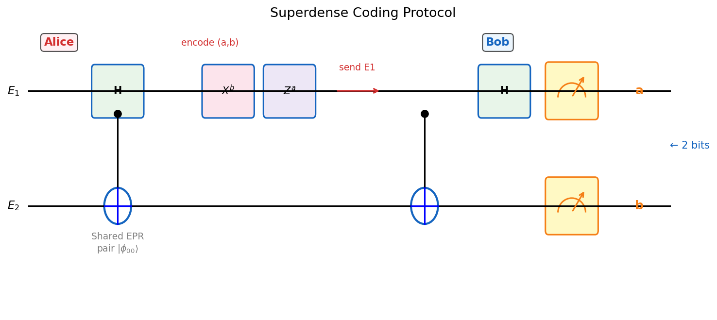
The key identity is \(|\phi_{ab}\rangle = (X^a Z^b \otimes I)|\phi_{00}\rangle\), so Alice’s encoding maps the shared state to exactly the Bell state \(|\phi_{ab}\rangle\), which Bob can identify by measuring in the Bell basis.
Physical intuition. The entanglement acts as a shared resource that amplifies the classical capacity of the quantum channel. Without the EPR pair, sending one qubit can transmit at most one classical bit (by Holevo’s theorem). The pre-shared entanglement doubles this capacity.
Importantly, no classical analogue of superdense coding exists. Moreover, without the pre-shared entanglement, local quantum operations alone cannot communicate any classical information.
4.2 Quantum Teleportation
Teleportation is the complementary protocol to superdense coding: while superdense coding uses one qubit to send two classical bits (doubling the classical capacity of a quantum channel), teleportation uses two classical bits to transmit one qubit (delivering a quantum channel through a classical channel). Together, these two protocols reveal a fundamental resource equivalence between quantum entanglement, quantum channels, and classical communication.
Alice transmits a quantum state to Bob by sending only two classical bits — again using a pre-shared EPR pair.
Theorem 2.2.1 (Teleportation). Suppose Alice and Bob share \(E_1, E_2\) in state \(|\phi_{00}\rangle = \frac{1}{\sqrt{2}}(|00\rangle + |11\rangle)\), and Alice has qubit \(M\) in state \(|\psi\rangle = \alpha|0\rangle + \beta|1\rangle\). Alice can help Bob construct \(|\psi\rangle\) by sending only 2 classical bits:
- Alice measures qubits \(ME_1\) in the Bell basis \(\{|\phi_{ab}\rangle : a,b \in \{0,1\}\}\).
- She sends the 2-bit outcome \((a,b)\) to Bob.
- Bob applies the correction operator \(X^a Z^b\) to \(E_2\).
- \(E_2\) is now in state \(|\psi\rangle\).
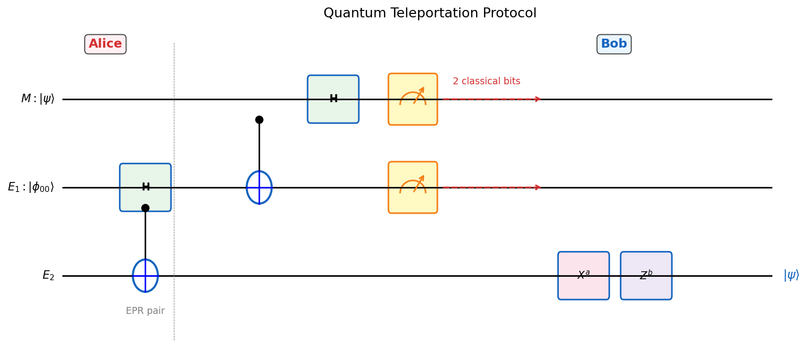
The proof works by expanding the joint state in the Bell basis and reading off the post-measurement states. The elegance of the protocol is that the four Bell-basis outcomes are equally probable (probability \(1/4\) each), regardless of the unknown state \(|\psi\rangle\) — so Alice’s measurement reveals nothing about \(|\psi\rangle\) to anyone, and the classical bits she sends to Bob merely tell him which correction to apply.
Proposition 2.2.2. After the teleportation protocol, the final state of \(E_2\) is \(|\psi\rangle\).
Example 2.2.3. Suppose Alice and Bob have an imperfect communication channel which applies the \(Z\) operator with probability 1% to any qubit sent over it. If Alice teleports \(|\psi\rangle\) and sends the 2 classical bits (possibly via superdense coding) through the channel, Bob can correctly apply the correction operator with arbitrarily high probability by repeating the classical transmission.
Physical intuition. Teleportation does not violate relativity: Alice must send classical bits to Bob before he can complete the recovery, so no information travels faster than light. The quantum state \(|\psi\rangle\) is “destroyed” at Alice’s end (her measurement collapses the state), so no copy is created — consistent with the no-cloning theorem.
Teleportation and superdense coding are dual: one converts one EPR pair + 1 qubit → 2 classical bits; the other converts one EPR pair + 2 classical bits → 1 quantum channel use. Together, they reveal the fundamental equivalence and interconvertibility of quantum and classical resources.
4.3 Quantum Key Distribution
Quantum Key Distribution (QKD) enables Alice and Bob to establish a shared secret key that is provably secure against any eavesdropper — with security guaranteed by quantum mechanics, not computational hardness assumptions.
This is a profound departure from all classical cryptography. Classical key distribution protocols — including RSA, Diffie-Hellman, and elliptic curve cryptography — base their security on the computational hardness of number-theoretic problems. A computationally unbounded adversary (or a large enough quantum computer) breaks all of them. QKD, by contrast, bases its security on two fundamental laws of quantum mechanics: the no-cloning theorem and the disturbance-upon-measurement principle. No adversary — regardless of computational power, even with a full quantum computer — can break a correctly implemented QKD protocol. The security is information-theoretic, not computational.
The threat model: Eve intercepts both the quantum and classical channels, is computationally unbounded, and knows the protocol. This is the strongest possible adversarial model, and yet QKD remains secure.
The key insight is that eavesdropping disturbs quantum states detectably. Here is the physical intuition in its starkest form. Suppose Alice sends a qubit in the state \(|+\rangle = \frac{1}{\sqrt{2}}(|0\rangle + |1\rangle)\). If Eve measures it in the computational basis, she collapses the state to either \(|0\rangle\) or \(|1\rangle\). When she forwards it to Bob, he receives a computational-basis state, not the original \(|+\rangle\). If Bob measures in the Hadamard basis (as he expected to), he now gets a random result — and when Alice and Bob compare results, they see an anomalous error rate. Eve cannot avoid this: she cannot learn anything about the qubit without interacting with it, and any interaction disturbs it, and any disturbance is statistically detectable. This is the physical core of QKD security, made mathematically precise by the security proof below. Any measurement Eve makes on the transmitted qubits introduces errors that Alice and Bob can detect by comparing a random subset of their received bits.
- Alice prepares \(k\) Bell pairs \(|\phi_{00}\rangle^{\otimes k}\) in registers \(A_1 B_1\).
- Alice encodes \(B_1\) with a CSS quantum error-correcting code \(C\) tolerating error rate \(\epsilon\), producing register \(B_1'\).
- Alice prepares \(n\) check Bell pairs in \(A_2 B_2\).
- Alice randomly permutes and sends all qubits \(B_1' \cup B_2\) to Bob.
- After Bob acknowledges receipt, Alice reveals the permutation.
- Alice selects a random string \(S \in \{0,1\}^n\); both measure check qubits \(B_2\) in standard basis (if \(S_i = 0\)) or Hadamard basis (if \(S_i = 1\)).
- If the observed error fraction exceeds threshold \(\epsilon - \nu\), output FAIL.
- Bob decodes \(B_1'\) using CSS error correction; both measure \(A_1, B_1\) to obtain key bits \(K_A, K_B\).
The security argument proceeds in two parts. When there is no eavesdropper, the protocol outputs PASS and \(K_A = K_B\) uniformly distributed over \(\{0,1\}^k\). When an eavesdropper is present and applies bit-flip or phase-flip errors, Alice and Bob detect these errors through the check qubits with probability exponentially close to 1 (by the Hoeffding bound), and either output FAIL or produce a key about which Eve has negligible information.
where \(H\) is the binary entropy function. This bound is used to control the probability of Alice and Bob failing to detect an eavesdropper.
Proposition 6.1.2. Suppose Eve applies a unitary operator \(U := P \otimes V\) to the \(2n\) qubits sent by Alice and a private register \(E\), where \(P := \bigotimes_{i=1}^{2n} P_i\) with each \(P_i \in \{I, X, Z, XZ\}\). If at least \(2\varepsilon n\) of the \(P_i \in \{X, XZ\}\), then Alice and Bob output FAIL with probability at least \(1 - 2e^{-cn}\) for a positive constant \(c\) depending only on \(\varepsilon, \nu\).
The use of CSS codes is essential: they can correct both bit-flip errors (in the standard basis) and phase-flip errors (in the Hadamard basis) simultaneously, which is required because Alice and Bob cannot measure both bases simultaneously on the same qubit.
It is worth pausing to understand why both bit-flip and phase-flip errors matter in QKD. Eve can attack in two ways. She can intercept a qubit and measure it in the computational basis — this introduces bit-flip errors detectable in the standard-basis check qubits. Or she can measure in the Hadamard basis — this introduces phase-flip errors detectable in the Hadamard-basis check qubits. Alice and Bob check both by randomly choosing between the two bases for each check qubit (via the random string \(S\)). A sophisticated adversary would try to hide between the two types of errors, but the CSS error correction structure ensures that any error pattern affecting more than a \(\varepsilon\) fraction of qubits in either basis will be detected. The no-cloning theorem makes it impossible for Eve to make a perfect copy and measure the copy later — any information Eve gains necessarily disturbs the original. This combination of physical law and algebraic structure is what gives QKD its unconditional security guarantee.
Chapter 5: Quantum Algorithms
Chapter 5 is the algorithmic heart of the course. Starting from the query model, we develop four landmark quantum algorithms — Deutsch-Jozsa, Simon’s, Shor’s, and Grover’s — each illustrating a different way that quantum mechanics provides computational advantages over classical methods.
5.1 The Query Model and Oracle Access
Many quantum algorithms are formulated in the query model (or black-box model): the algorithm has access to an oracle \(O_f\) that computes some function \(f\), and the goal is to determine a property of \(f\) using as few queries as possible. The query complexity captures the inherent algorithmic difficulty independently of implementation details, making it the cleanest setting for proving quantum advantages.
Example 4.1.1. Given a Boolean formula \(\varphi\) over \(n\) variables in CNF, an assignment \(a \in \{0,1\}^n\) satisfies \(\varphi\) if \(\varphi(a) = 1\). A classical circuit \(C_\varphi\) or quantum circuit \(O_\varphi\) checking whether a given assignment satisfies \(\varphi\) is an oracle with domain \(D = \{0,1\}^n\). The number of queries needed to determine satisfiability is the query complexity.
Unlike classical oracles, the quantum oracle can be queried in superposition, allowing the algorithm to “see” many inputs simultaneously.
5.2 The Deutsch-Jozsa Algorithm
The Deutsch-Jozsa algorithm is historically the first quantum algorithm to demonstrate an exact (not just approximate) exponential separation between quantum and classical query complexity. While the problem it solves is artificial, it establishes the key technique of quantum interference that all later algorithms exploit.
Problem 1 (Deutsch-Jozsa). Given an oracle for \(f : \{0,1\}^n \to \{0,1\}\) promised to be either constant (same output on all inputs) or balanced (output 0 on exactly half the domain), determine which it is.
Classically, \(2^{n-1} + 1\) queries are needed in the worst case — you might check half the inputs and still not be sure. Quantum mechanically, the structure of the function is revealed in a single measurement, after two queries.
Theorem 4.2.1 (Deutsch-Jozsa). There is a quantum algorithm DJ making 2 oracle queries that gives the correct output with probability 1.
The algorithm applies \(H^{\otimes n}\) to \(|0^n\rangle\), queries the oracle (twice using the phase kickback trick), then applies \(H^{\otimes n}\) again. The key insight is the Hadamard transform identity:
\[H^{\otimes n}|x\rangle = \frac{1}{\sqrt{2^n}}\sum_{y \in \{0,1\}^n} (-1)^{x \cdot y} |y\rangle,\]where \(x \cdot y = \bigoplus_{i=1}^n x_i y_i\). After two oracle queries, the \(|0^n\rangle\) component has amplitude \(\pm 1\) if \(f\) is constant, and amplitude 0 if \(f\) is balanced.
This identity is the heart of the Deutsch-Jozsa algorithm: constant functions give all amplitudes aligned, while balanced functions have cancellation leaving zero amplitude on \(|0^n\rangle\).
Versus randomized classical. A randomized algorithm sampling 2 random inputs solves the problem with one-sided error at most \(1/2\). By repeating \(t\) times, the error is \(1/2^t\). So a randomized algorithm with \(O(\log(1/\varepsilon))\) queries achieves error \(\varepsilon\) — comparable to the quantum algorithm asymptotically. The quantum advantage here is exact versus approximate, not asymptotic.
5.3 Simon’s Algorithm
Simon’s algorithm is the historical bridge between the Deutsch-Jozsa problem and Shor’s factoring algorithm. It demonstrates an exponential quantum speedup for a structured search problem and introduces the core idea of using quantum Fourier analysis to extract hidden algebraic structure.
Here is the key conceptual point that makes Simon’s problem so important. Classically, finding the hidden secret \(s\) is a search problem: you query the oracle on random inputs until two inputs collide — that is, until you find \(x \neq y\) with \(f(x) = f(y)\), at which point \(s = x \oplus y\). By the birthday paradox, this collision occurs after roughly \(\sqrt{2^n} = 2^{n/2}\) queries. And the lower bound theorem confirms this is tight — you cannot do better classically. Quantumly, however, you do not search for the secret directly. Instead, you prepare a superposition, query the oracle (which entangles the query register with the output register), and then apply the Hadamard transform. The measurement result is a random vector orthogonal to \(s\). Repeating \(O(n)\) times gives enough orthogonality constraints to pin down \(s\) exactly. The quantum algorithm learns about \(s\) not by finding it, but by sampling from its orthogonal complement — an entirely different strategy that has no classical counterpart.
Problem 2 (Simon). Given oracle access to \(f : \{0,1\}^n \to \{0,1\}^n\) that hides a secret \(s \in \mathbb{Z}_2^n\) in the sense that \(f(x) = f(y) \iff y = x \oplus s\), find \(s\).
Classically, finding \(s\) requires \(\Omega(2^{n/2})\) queries by a birthday-paradox argument. Simon’s quantum algorithm uses only \(O(n)\) queries — an exponential improvement — by sampling from the orthogonal complement of the hidden subgroup.
Theorem 4.3.1. There is a randomized algorithm that finds \(s\) with probability at least \(\frac{2}{3}\), using \(O(2^{n/2})\) queries to the oracle for \(f\).
Theorem 4.3.2. Any randomized algorithm that solves the Simon problem with success probability at least \(\frac{2}{3}\) requires \(\Omega(2^{n/2})\) queries.
These two theorems establish that the classical query complexity of Simon’s problem is \(\Theta(2^{n/2})\), making Simon’s quantum algorithm an exponential improvement. The lower bound is crucial: it rules out the possibility that some clever classical algorithm finds \(s\) without the birthday-paradox collision strategy, and it makes the quantum-classical separation unconditional in the query model — a rarity in complexity theory. This is one of the few places in the entire theory where we have a proven, unconditional exponential separation between quantum and classical computation.
Core subroutine. The SAMPLE(\(f\)) circuit applies \(H^{\otimes n}\) to \(|0^n\rangle\), queries the oracle, then applies \(H^{\otimes n}\) again. The key calculation shows:
\[H^{\otimes n}\left(\tfrac{1}{\sqrt{2}}(|x\rangle + |x \oplus s\rangle)\right) = \frac{1}{\sqrt{2^{n-1}}} \sum_{y \in S^\perp} (-1)^{x \cdot y}|y\rangle,\]where \(S^\perp = \{y \in \mathbb{Z}_2^n : y \cdot s = 0\}\) is the orthogonal complement of \(S = \{0^n, s\}\). Measuring gives a uniformly random element of \(S^\perp\).
Full algorithm:
- Run SAMPLE(\(f\)) for \(t = 8n\) times.
- Let \(Y_1, \ldots, Y_t\) be the outcomes. Solve \(\{Y_i \cdot w = 0\}\) over \(\mathbb{Z}_2\) by Gaussian elimination.
- The unique non-zero solution is \(s\).
Proposition 4.3.3. Let \(Y_1, Y_2, \ldots, Y_t\) be i.i.d. random variables uniform over the subspace \(S^\perp\). Then the probability that the \(Y_i\)’s span \(S^\perp\) when \(t = 8n\) is at least \(\frac{3}{4}\).
Theorem 4.3.4 (Simon’s Algorithm). Simon’s algorithm has query complexity \(O(n)\), uses \(O(n^2)\) qubits and \(O(n^2)\) quantum gates, with classical post-processing using \(O(n^2)\) bits and time \(O(n^3)\). It produces output \(\tilde{s}\) with probability at least \(\frac{3}{4}\), and \(P(\tilde{s} = s \mid \text{not fail}) = 1\).
The proof reduces to a linear-algebraic argument: enough random vectors in a subspace eventually span it, and the probability of success is controlled by a standard coupon-collector bound.
When Peter Shor saw Simon’s algorithm in 1994, he recognized that factoring could be reduced to a similar hidden-period problem over the integers. The connection is profound: if you want to factor \(n\), pick a random \(a\) and look at the sequence \(a^0, a^1, a^2, \ldots\) modulo \(n\). This sequence is periodic with period \(r\) (the order of \(a\) modulo \(n\)), and knowing \(r\) lets you extract a nontrivial factor of \(n\) via a simple GCD computation. Finding \(r\) classically is as hard as factoring, but quantumly it reduces to Simon’s core idea: query a superposition, measure the output to collapse into a periodic state, and then use the Fourier transform to read off the period. Simon’s algorithm was the proof of concept that this strategy works; Shor’s algorithm was its full realization.
Simon’s algorithm is the historical precursor to Shor’s factoring algorithm: both solve a hidden subgroup problem (HSP) over an abelian group (\(\mathbb{Z}_2^n\) for Simon, \(\mathbb{Z}\) for period-finding).
The Hidden Subgroup Framework. The Simon problem is a special case of the HSP: given a group \(G\) and a function \(f : G \to S\) that is constant and distinct on cosets of a hidden subgroup \(H \leq G\), find \(H\). Simon’s algorithm applies to \(G = \mathbb{Z}_2^n\), \(H = \{0, s\}\). Shor’s period-finding applies to \(G = \mathbb{Z}\), \(H = r\mathbb{Z}\). Both use the quantum Fourier transform on \(G\) to sample uniformly from the dual group \(H^\perp\), then classically recover \(H\) from enough dual samples. The abelian HSP is efficiently solvable on a quantum computer for any finite abelian group. The non-abelian HSP (e.g., the symmetric group \(S_n\), which would give a quantum algorithm for graph isomorphism) remains open and is a major research frontier.
5.4 Phase Estimation and Quantum Fourier Transform
Phase estimation is the crucial subroutine that connects the quantum Fourier transform to eigenvalue problems — and from there to factoring. The idea is to “read out” the eigenvalue of a unitary by encoding it in the phase of a quantum state and then using the QFT to decode it.
To understand why this is powerful, recall the classical analogy. If you want to know the frequency of a signal, you listen for a long time and apply the Fourier transform — a longer observation window gives finer frequency resolution. Phase estimation is the quantum version of this procedure. The “signal” is the action of repeated applications of a unitary \(U\), and the “frequency” is the phase \(\theta\) of the eigenvalue \(e^{2\pi i\theta}\). By applying \(U^1, U^2, U^4, \ldots, U^{2^{m-1}}\) in a controlled fashion (using \(m\) ancilla qubits in superposition), you build up a quantum state whose Fourier coefficients encode \(\theta\). Applying the inverse QFT then produces a measurement outcome that is an \(m\)-bit approximation to \(\theta\). The key quantum advantage is that you can prepare all \(m\) powers simultaneously through controlled-\(U\) gates, giving an \(O(m)\)-query algorithm that would require exponential resources classically.
Phase estimation is not just a subroutine for Shor’s algorithm — it is the central primitive for a whole landscape of quantum algorithms: it underlies quantum simulation (estimating energy eigenvalues of a Hamiltonian), quantum linear systems algorithms (HHL), and quantum principal component analysis. Understanding phase estimation deeply is understanding the engine of most of practical quantum computation.
Phase estimation is the central subroutine in Shor’s algorithm and eigenvalue estimation.
Problem 3 (Phase Estimation). Given a unitary \(U = \begin{pmatrix}1 & 0 \\ 0 & e^{2\pi i\theta}\end{pmatrix}\) (with circuits for \(U^{2^k}\)) and accuracy \(\varepsilon \in (1/2^m, 1)\), output an estimate \(\tilde\theta\) such that \(|\theta - \tilde\theta| \leq \varepsilon\).
The QFT is the quantum analogue of the classical Discrete Fourier Transform, implemented exponentially faster: a classical DFT on \(2^m\) points requires \(O(m 2^m)\) operations, while the QFT requires only \(O(m^2)\) quantum gates. This exponential speedup is one of the core quantum advantages.
The Fourier basis \(\{|\chi_x\rangle\}\) is orthonormal. If \(\theta = a/2^m\) exactly, measuring the state \(|\psi_\theta\rangle = \frac{1}{\sqrt{2^m}}\sum_y e^{2\pi i\theta y}|y\rangle\) in the Fourier basis yields outcome \(a\) with probability 1.
Theorem 4.4.1 (Kitaev). Given circuits for applying \(U^{2^k}\) where \(U = \begin{pmatrix}1 & 0 \\ 0 & e^{2\pi i\theta}\end{pmatrix}\) for \(k \in [m]\), we can learn \(\theta\) up to \(m\) bits of precision using \(O(m)\) qubits and \(O(m)\) other gates and measurements.
Notice the remarkable efficiency: \(m\) bits of precision from \(m\) qubits and \(m\) queries. Classically, learning a number to \(m$ bits of precision naively requires \(2^m\) function evaluations. The quantum Fourier transform compresses all of this into a single measurement after \(m\) controlled-unitary applications. This is the heart of the exponential speedup for period-finding and eigenvalue estimation.
This geometric inequality is used in the analysis of the phase estimation success probability.
Theorem 4.5.1. There is a quantum circuit for \(F_{2^m}\) over \(\mathbb{Z}_{2^m}\) that uses \(m\) qubits, has no measurements, and has \(O(m^2)\) single- or two-qubit gates.
The circuit applies controlled phase gates \(R_j = \begin{pmatrix}1&0\\0&e^{2\pi i/2^j}\end{pmatrix}\) in a structured pattern, analogous to the classical Fast Fourier Transform.
5.5 Eigenvalue Estimation and Period Finding
Eigenvalue estimation generalizes phase estimation to arbitrary unitaries: given \(V|\psi\rangle = e^{2\pi i\theta}|\psi\rangle\), estimate \(\theta\). The circuit combines \(H^{\otimes m}\), controlled-\(V^x\) operations, and the inverse QFT \(F_{2^m}^\dagger\).
It is worth stepping back to appreciate the scope of this subroutine. Eigenvalue estimation is the quantum analogue of computing the spectrum of an operator — one of the most fundamental tasks in all of mathematics. Classically, computing eigenvalues of an \(N \times N\) matrix requires at least \(\Omega(N)\) operations, and for exponentially large matrices (like the Hamiltonian of a physical system), this is simply intractable. Quantumly, if the matrix \(V\) can be implemented as a quantum circuit, eigenvalue estimation runs in time polynomial in the number of qubits — an exponential speedup. This is why quantum simulation of physical systems (quantum chemistry, condensed matter) is one of the most promising near-term applications of quantum computers: the Hamiltonians of molecular systems are precisely the kind of operators for which eigenvalue estimation gives an exponential advantage. It is also why HHL — the quantum linear systems algorithm — can achieve exponential speedups: solving \(Ax = b\) can be reduced to eigenvalue estimation on \(A\). Phase estimation is not a curiosity; it is the engine of practical quantum advantage.
Theorem 4.6.1. Let \(m := \lfloor\log(1/\varepsilon)\rfloor\). With probability at least \(\frac{1}{4}\), the eigenvalue estimation circuit produces an estimate \(\tilde\theta \in [0,1)\) such that \(|\theta - \tilde\theta| \leq \varepsilon\), when \(|\psi\rangle\) is an eigenvector of \(V\) with eigenvalue \(e^{2\pi i\theta}\).
Period finding reduces to eigenvalue estimation via the following insight: if \(a\) has order \(r\) modulo \(n\), define
\[|ψ_k\rangle = \frac{1}{\sqrt{r}} \sum_{j=0}^{r-1} \omega^{-kj} |a^j \bmod n\rangle, \quad \omega = e^{-2\pi i/r}.\]This state satisfies \(V_a|ψ_k\rangle = e^{2\pi ik/r}|\psi_k\rangle\), where \(V_a: |x\rangle \mapsto |ax \bmod n\rangle\). Furthermore, \(|1\rangle = \frac{1}{\sqrt{r}}\sum_{k=0}^{r-1}|\psi_k\rangle\), so initializing with \(|1\rangle\) and running eigenvalue estimation gives an approximation \(\tilde\theta_k \approx k/r\). From \(\tilde\theta_k\), the classical continued fractions algorithm recovers \(r\) when \(\gcd(k,r) = 1\).
The continued fractions step is a beautiful piece of classical number theory. The algorithm produces a floating-point approximation \(\tilde\theta_k \approx k/r\) accurate to about \(\log n\) bits. Among all fractions \(p/q\) with denominator \(q \leq n\), there is at most one fraction within \(1/(2n^2)\) of any given real number — a classical theorem. So if \(\tilde\theta_k\) is close enough to \(k/r\), the continued fractions algorithm uniquely identifies \(k/r\) and hence \(r\). The only remaining requirement is that \(\gcd(k,r) = 1\) (so that the fraction \(k/r\) is in lowest terms, with denominator exactly \(r\)). Euler’s totient function guarantees that a constant fraction of values \(k\) are coprime with \(r\), so a constant number of repetitions suffice. The quantum computer does the exponentially hard part — finding the period — while classical number theory does the polynomial cleanup.
Lemma 4.7.1. Let \(1 < n \in \mathbb{Z}\) and \(\gcd(a,n) = 1\). The function \(f_a : \mathbb{Z}_n \to \mathbb{Z}_n\) given by \(f_a(x) := ax \bmod n\) is invertible.
Proposition 4.7.2. The number of \(k \in [r-1]\) that are coprime with \(r\) is \(\Omega(r / \log\log r)\). Hence repeating the sampling procedure \(O(\log\log r) \subseteq O(\log\log n)\) times, we sample \(\tilde\theta_k\) for \(k\) coprime with \(r\) at least once with high probability.
Theorem 4.7.3. There is a polynomial-time algorithm that outputs the order of \(a \bmod n\) with probability at least \(\frac{2}{3}\). Moreover, the algorithm makes no incorrect outputs and outputs “FAIL” if it fails to find the order.
5.6 Shor’s Factoring Algorithm
Shor’s algorithm is arguably the most important result in quantum computing. By reducing factoring to period finding, and period finding to phase estimation via the QFT, it achieves a superpolynomial speedup over all known classical algorithms — with immediate implications for the security of virtually all modern cryptosystems.
Problem 5 (Integer Factorization). Given integer \(n > 1\), output “prime”, or \(1 < n_1 < n\) such that \(n_1 \mid n\).
No polynomial-time classical algorithm for factoring is known. The best known algorithm (the General Number Field Sieve) runs in time \(\exp\left(O((\log n)^{1/3}(\log\log n)^{2/3})\right)\) — sub-exponential but far from polynomial.
Theorem 4.8.1. If the integer \(n > 1\) has at least two distinct prime factors, then at least a constant fraction of numbers \(a \in \mathbb{Z}_n^*\) satisfy the following property: letting \(r := |a|\) be the order of \(a \bmod n\), \(r\) is even and \(a^{r/2} - 1\) has a non-trivial factor in common with \(n\).
Theorem 4.8.2 (Shor). There is an efficient quantum algorithm for integer factorization that computes all the prime factors of a given integer \(n\), in time \(\mathrm{poly}(\log n)\), with probability at least \(\frac{2}{3}\).
This is a polynomial-time algorithm on a quantum computer for a problem that is believed to require superpolynomial time classically. It is the strongest evidence that \(BQP \not\subseteq BPP\) — though no formal proof of this separation is known.
The reduction from factoring to period finding works as follows. For \(n\) with at least two distinct prime factors, a constant fraction of \(a \in \mathbb{Z}_n^*\) have the property that the order \(r = |a|\) is even and \(\gcd(a^{r/2} - 1, n) > 1\). The algorithm: pick \(a\) at random, compute \(r\) using period finding, check if \(r\) is even and \(\gcd(a^{r/2}-1, n) \notin \{1, n\}\).
Security implications. Shor’s algorithm breaks RSA encryption and discrete-log based cryptosystems (ECC, DSA). This motivates the field of post-quantum cryptography, which designs classical cryptosystems secure against quantum adversaries.
5.7 The Discrete Logarithm Problem
The discrete logarithm problem (DLP) is, alongside integer factoring, one of the pillars on which modern public-key cryptography rests. Diffie–Hellman key exchange, the Digital Signature Algorithm, and elliptic-curve cryptography all derive their security from the presumed classical hardness of computing discrete logarithms. Like factoring, the DLP yields to the quantum toolkit — specifically, to a double application of eigenvalue estimation.
Problem 7 (Discrete Logarithm). Let \(G\) be a finite cyclic group of known order \(r\), with generator \(a\). Given \(b \in G\) such that \(b = a^s\) for some \(s \in \{0, 1, \ldots, r-1\}\), find \(s\).
Classically, the best generic algorithm (baby-step giant-step, or Pollard’s rho) runs in time \(O(\sqrt{r})\). No polynomial-time classical algorithm is known. On a quantum computer, the DLP can be solved in polynomial time by combining two eigenvalue estimation subroutines.
Eigenvector structure. Define the unitary \(U_a : |x\rangle \mapsto |ax\rangle\). Because \(a\) has order \(r\), the operator \(U_a\) has eigenvectors
\[|\psi_k\rangle = \frac{1}{\sqrt{r}} \sum_{j=0}^{r-1} e^{-i2\pi jk/r} |a^j\rangle, \qquad k = 0, 1, \ldots, r-1,\]with eigenvalues \(e^{i2\pi k/r}\). The key insight is that the unitary \(U_b : |x\rangle \mapsto |bx\rangle\) shares the same eigenvectors. Since \(b = a^s\):
\[U_b |\psi_k\rangle = e^{i2\pi ks/r} |\psi_k\rangle.\]Proposition 4.11.1. The eigenvectors \(|\psi_k\rangle\) of \(U_a\) are simultaneously eigenvectors of \(U_b\). The eigenvalue of \(U_a\) on \(|\psi_k\rangle\) is \(e^{i2\pi k/r}\), and the eigenvalue of \(U_b\) on \(|\psi_k\rangle\) is \(e^{i2\pi ks/r}\).
The algorithm. The circuit uses two control registers and one target register initialized to \(|1\rangle\):
- Prepare both control registers in uniform superposition via \(H^{\otimes m}\).
- Using the first control register, apply controlled-\(U_a^x\) to the target.
- Using the second control register, apply controlled-\(U_b^y\) to the target.
- Apply inverse QFT to each control register independently.
- Measure both control registers to obtain estimates of \(k/r\) and \(ks/r\).
Classical post-processing via continued fractions recovers \(k\) and \(ks \bmod r\). When \(\gcd(k, r) = 1\), we compute \(s = (ks) \cdot k^{-1} \bmod r\).
Theorem 4.11.2 (Shor). There is an efficient quantum algorithm for the discrete logarithm problem that outputs \(s\) in time \(\mathrm{poly}(\log r)\) with probability at least \(\frac{2}{3}\).
Cryptographic implications. Just as Shor’s factoring algorithm breaks RSA, the discrete logarithm algorithm breaks Diffie–Hellman key exchange, DSA, and elliptic-curve cryptography, further motivating the transition to post-quantum cryptographic primitives.
5.8 Grover’s Search Algorithm
Grover’s algorithm provides a quadratic quantum speedup for unstructured search — one of the most fundamental problems in computing. Unlike Shor’s algorithm, which exploits specific algebraic structure (periodicity), Grover’s algorithm works for any search problem, making its quadratic speedup universal.
The geometric picture is the key to understanding why Grover’s algorithm works. Think of two unit vectors in a two-dimensional plane: the target state \(|a\rangle\) (the “answer”) and the uniform superposition \(|u\rangle\) (where we start). Our goal is to rotate from \(|u\rangle\) toward \(|a\rangle\). The initial angle between \(|u\rangle\) and the subspace orthogonal to \(|a\rangle\) is very small — roughly \(\theta \approx 1/\sqrt{N}\) for \(N = 2^n\) items. Each iteration of the Grover operator rotates the state by \(2\theta\) toward \(|a\rangle\). After about \(\pi/(4\theta) \approx \pi\sqrt{N}/4\) iterations, the state has rotated to \(|a\rangle\), and measuring yields the correct answer with near-certainty. This geometric picture immediately explains both the correctness and the optimality: to move an angle of order 1 in steps of size \(1/\sqrt{N}\) requires \(O(\sqrt{N})\) steps.
Problem 6 (Unordered Search). Given oracle access to \(f : \{0,1\}^n \to \{0,1\}\), output 1 if there is some \(a\) such that \(f(a) = 1\), and 0 otherwise.
Classically, this requires \(\Omega(2^n)\) queries in the worst case — every element must potentially be checked. Remarkably, the quantum speedup is exactly quadratic and provably optimal.
Definition 4.9.1 (Non-Deterministic Polynomial Time). The complexity class \(\mathbf{NP}\) consists of computational problems for which, given a potential solution, one can verify it is valid efficiently (in polynomial time).
Theorem 4.9.1 (Bennett, Bernstein, Brassard, Vazirani). Any quantum algorithm for the unordered search problem with oracle access requires \(\Omega(2^{n/2})\) queries.
The lower bound proof is a hybrid argument: it tracks how quickly the quantum state can “learn” the location of the marked element by measuring the distance between executions on different oracles. This style of argument — comparing the algorithm’s state on two nearly identical oracles — is a fundamental tool in quantum query complexity.
Theorem 4.9.2 (Grover). There is a quantum algorithm for the unordered search problem with query complexity \(O(2^{n/2})\) and \(O(n \cdot 2^{n/2})\) other single/two-qubit gates. Moreover, the algorithm makes no error when \(f \equiv 0\), and makes error at most \(\frac{1}{3}\) otherwise.
Theorem 4.9.3. Any classical algorithm for element distinctness (given \(x_1, \ldots, x_n \in [n]\), decide if all are distinct) requires \(\Omega(n \log n)\) comparisons. A straightforward application of Grover search solves element distinctness in \(O(n)\) queries; a more sophisticated quantum algorithm achieves the optimum \(O(n^{2/3})\) comparisons.
The algorithm. The core idea is to rotate the initial uniform superposition \(|u\rangle = H^{\otimes n}|0^n\rangle\) towards the marked state \(|a\rangle\):
- Initialize \(|u\rangle = \frac{1}{\sqrt{2^n}}\sum_x |x\rangle\) and prepare ancilla in \(|-\rangle\).
- Apply \(t = \lfloor\pi/4\theta\rfloor\) iterations of the Grover operator \(G = R \cdot R_f\):
- Phase oracle \(R_f = I - 2|a\rangle\langle a|\): flips the sign of the marked state (using phase kickback with the \(|-\rangle\) ancilla).
- Diffusion operator \(R = 2|u\rangle\langle u| - I\): reflects about the uniform superposition, implemented as \(H^{\otimes n}(2|0^n\rangle\langle 0^n| - I)H^{\otimes n}\).
- Measure the query register; output 1 if \(f(\text{outcome}) = 1\).
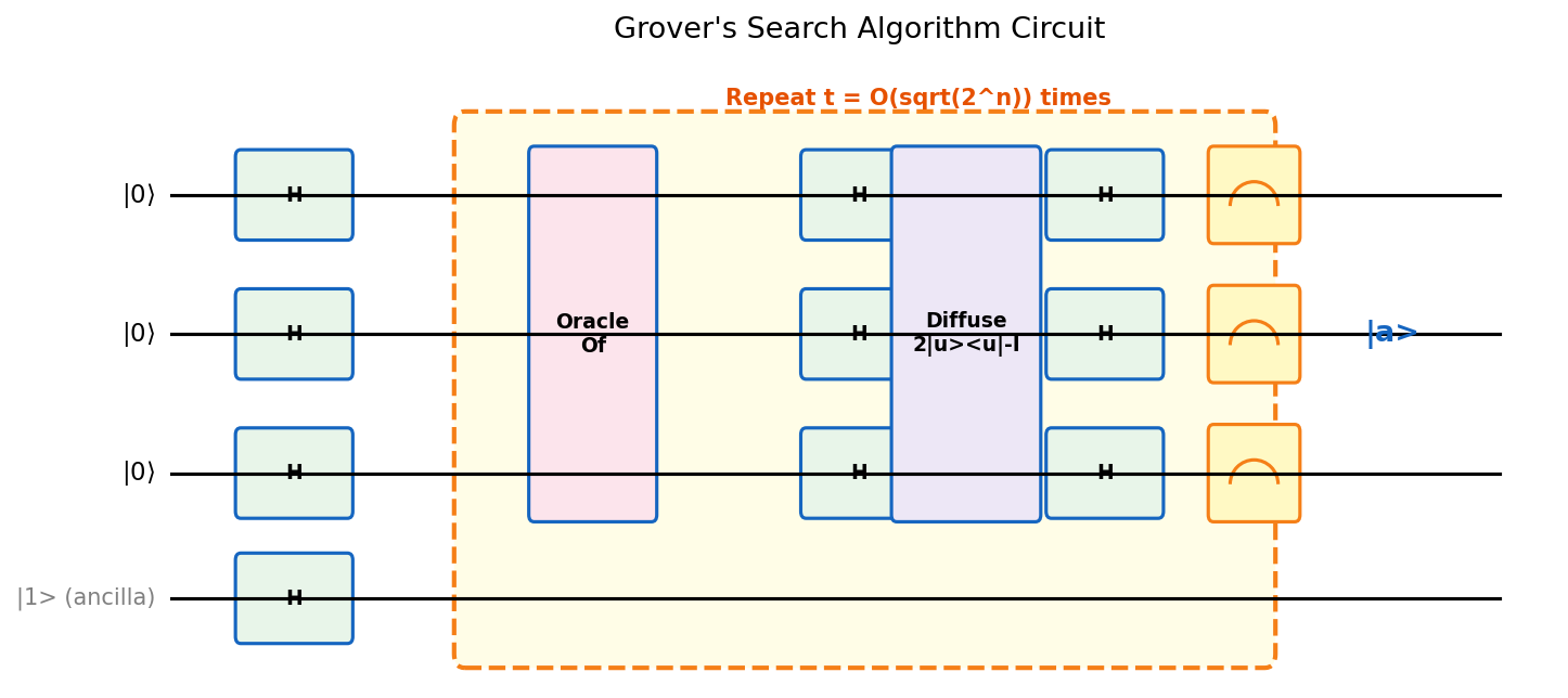
The two lemmas below make the geometric picture rigorous. Lemma 4.10.1 shows that the diffusion operator — the reflection about \(|u\rangle\) — can be implemented cheaply. It is built from a reflection about \(|0^n\rangle\) conjugated by Hadamards, costing only \(O(n)\) gates with no oracle queries at all. Lemma 4.10.2 is the core geometric result: it proves that the composition \(G = R \cdot R_f\) of two reflections is a rotation, and it computes the rotation angle exactly. Two reflections always compose to a rotation — this is a classical fact from Euclidean geometry — but the beauty here is that the rotation angle \(2\theta\) is determined entirely by the initial overlap \(\sin\theta = 1/\sqrt{N}\) between the uniform superposition and the target state. Together, these two lemmas provide a complete and elementary proof of Grover’s correctness.
without any queries to \(f\), using \(O(n)\) single- and two-qubit gates.
The reflection about \(|0^n\rangle\) is implemented by conjugating a multi-controlled Z gate with single-qubit X gates: first flip all bits so that \(|0^n\rangle\) maps to \(|1^n\rangle\), apply a \((n-1)\)-controlled Z gate that phases \(|1^n\rangle\) by \(-1\), then flip the bits back. The global minus sign on all \(|x\rangle \neq |0^n\rangle\) is equivalent to a single minus sign on \(|0^n\rangle\) up to a global phase, which is all we need.
through angle \(2\theta\) (in the basis \(|a\rangle, |v\rangle\)), and as \(-I\) on \(V^\perp\).
This lemma is the geometric heart of Grover’s algorithm. The key insight is that the initial state \(|u\rangle\) lies in the 2D subspace \(V = \text{span}\{|a\rangle, |v\rangle\}\), and both reflections \(R_f\) and \(R\) preserve this subspace. Therefore, all of Grover’s dynamics are confined to a 2D plane — regardless of how large \(N\) is — and the algorithm is equivalent to a single rotation problem in that plane. The rotation angle \(2\theta\) satisfies \(\sin\theta = 1/\sqrt{N}\), so \(\theta \approx 1/\sqrt{N}\) and it takes approximately \(\pi/(4\theta) = O(\sqrt{N})\) rotations to reach \(|a\rangle\) from \(|u\rangle\). The proof that \(G\) acts as \(-I\) on the orthogonal complement \(V^\perp\) ensures that no amplitude leaks out of the relevant 2D subspace.
Correctness. The operator \(G = RR_f\) acts as a rotation by angle \(2\theta\) (where \(\sin\theta = 1/\sqrt{2^n}\)) in the 2D subspace \(\operatorname{span}\{|a\rangle, |v\rangle\}\). After \(t\) iterations, the state of the query register is \(\sin((2t+1)\theta)|a\rangle + \cos((2t+1)\theta)|v\rangle\). With \(t = \lfloor\pi/(4\theta)\rfloor\), the angle \((2t+1)\theta \approx \pi/2\), giving success probability \(\sin^2((2t+1)\theta) \geq 1 - 1/2^n\).
This correctness argument reveals an important subtlety: the algorithm must stop at exactly the right step. If you run too many iterations, the state rotates past \(|a\rangle\) and the success probability starts decreasing again. This is fundamentally unlike classical search, where adding more computation never hurts. The quadratic speedup is therefore precise: \(t = \lfloor\pi\sqrt{N}/4\rfloor\) steps, not more and not fewer. For multiple marked elements (say \(m\) out of \(N\) total), the rotation angle becomes \(\sin\theta = \sqrt{m/N}\), and the algorithm terminates in \(O(\sqrt{N/m})\) steps — a continuous tradeoff between the density of solutions and the query complexity. This multi-solution generalization is practically important: most real search problems have many valid solutions, and Grover’s algorithm adapts gracefully.
Applications. Grover’s algorithm gives a quadratic speedup for any brute-force search. For domain of size \(m\), the query complexity is \(O(\sqrt{m})\). This has immediate implications: element distinctness can be solved in \(O(n)\) queries (vs. \(\Omega(n\log n)\) classically), and many combinatorial optimization problems admit Grover-based speedups.
5.9 Quantum Counting and Amplitude Estimation
Grover’s algorithm assumes we know (at least approximately) how many solutions exist — the optimal number of iterations depends on the fraction of marked elements. What if the number of solutions is unknown? And can we count the number of solutions quantumly? Both questions are answered by amplitude estimation, which reduces counting and probability estimation to phase estimation on the Grover operator.
The amplitude estimation framework. Suppose a quantum circuit \(A\) satisfies
\[A|0\rangle = \sin(\theta)|{\Psi_1}\rangle|1\rangle + \cos(\theta)|{\Psi_0}\rangle|0\rangle.\]The goal is to estimate \(\sin^2(\theta)\). The Grover operator \(Q = -A S_0 A^{-1} S_\chi\) has eigenvalues \(e^{\pm i2\theta}\) in the relevant two-dimensional subspace, and the initial state \(A|0\rangle\) is a superposition of the two eigenvectors. Applying phase estimation to \(Q\) yields an estimate of \(\theta\) and hence \(\sin^2(\theta)\).
Theorem 4.12.2 (Brassard, Hoyer, Mosca, Tapp). There is a quantum algorithm that estimates \(\sin^2(\theta)\) to additive accuracy \(\varepsilon\) using \(O(1/\varepsilon)\) applications of \(A\) and \(A^{-1}\), with success probability at least \(\frac{2}{3}\).
This is a quadratic improvement over the classical \(\Theta(1/\varepsilon^2)\) sample complexity. The speedup arises because phase estimation extracts information from the eigenvalue structure of the Grover operator rather than simply sampling and averaging.
Application to quantum counting. Given an oracle \(f : \{0,1\}^n \to \{0,1\}\), let \(t = |\{x : f(x) = 1\}|\) and \(N = 2^n\). Using the standard Grover setup, \(\sin^2(\theta) = t/N\), so amplitude estimation gives an estimate of \(t\).
Theorem 4.12.3 (Quantum Counting). Given oracle access to \(f:\{0,1\}^n \to \{0,1\}\) with \(t\) marked elements among \(N = 2^n\), there is a quantum algorithm that estimates \(t\) to additive accuracy \(\varepsilon N\) using \(O(1/\varepsilon)\) oracle queries.
Exact counting requires distinguishing \(\sqrt{t/N}\) from \(\sqrt{(t+1)/N}\), which needs precision \(O(1/\sqrt{tN})\). By the amplitude estimation bound, this requires \(O(\sqrt{tN})\) queries. A symmetrized analysis shows exact counting requires \(O(\sqrt{t(N-t)})\) queries — tight up to constants.
Searching without knowing the number of solutions. Amplitude estimation resolves the practical difficulty that Grover’s optimal iteration count depends on the unknown \(t\): first estimate \(t\) to sufficient precision, then run Grover’s algorithm with the correct number of iterations. This achieves expected query complexity \(O(\sqrt{N/t})\) — matching Grover when \(t\) is known.
5.10 The Hidden Subgroup Problem
The quantum algorithms we have studied — Deutsch–Jozsa, Simon, order finding, discrete logarithm, and factoring — all share a common algebraic backbone: each finds a hidden subgroup of some group. The hidden subgroup problem (HSP) provides a unifying framework that clarifies why these algorithms work and identifies the frontier of quantum algorithmic power.
Definition 4.13.1 (Hidden Subgroup Problem). Let \(G\) be a finitely generated group, \(X\) a finite set, and \(f : G \to X\) a function satisfying \(f(x) = f(y)\) if and only if \(xS = yS\) for some subgroup \(S \leq G\). Given oracle access to \(f\), determine a generating set for \(S\).
Every quantum algorithm in this chapter that achieves a superpolynomial speedup is an instance of the HSP:
- Deutsch–Jozsa: \(G = \mathbb{Z}_2\), \(S = \mathbb{Z}_2\) (constant) or \(S = \{0\}\) (balanced).
- Simon’s problem: \(G = \mathbb{Z}_2^n\), \(S = \{0^n, s\}\).
- Order finding: \(G = \mathbb{Z}\), \(f(x) = a^x \bmod N\), \(S = r\mathbb{Z}\).
- Discrete logarithm: \(G = \mathbb{Z}_r \times \mathbb{Z}_r\), \(f(x,y) = a^x b^y\), \(S = \langle(1, -s)\rangle\).
Theorem 4.13.2 (Abelian HSP). Let \(G\) be a finite abelian group. There is an efficient quantum algorithm that solves the hidden subgroup problem over \(G\) using \(\mathrm{poly}(\log |G|)\) queries and gates.
The algorithm generalizes the approach of Simon’s and Shor’s algorithms: (1) prepare a uniform superposition over \(G\) and query the oracle to collapse onto a random coset of \(S\), (2) apply the QFT over \(G\) to convert the coset state into a random element of the annihilator \(S^\perp\), (3) repeat \(O(\log|G|)\) times and reconstruct \(S\) from \(S^\perp\) via Gaussian elimination.
The non-abelian frontier. When \(G\) is non-abelian, the situation changes dramatically. The key open case is the symmetric group \(S_n\): an efficient quantum algorithm for the HSP over \(S_n\) would yield an efficient algorithm for graph isomorphism and graph automorphism. Despite substantial effort, the standard Fourier sampling approach provably fails for \(S_n\), and the problem remains one of the most important open questions in quantum computing.
5.11 Query Complexity Lower Bounds
Grover’s algorithm finds a marked item among \(N\) elements using \(O(\sqrt{N})\) queries. Can we do better? The theory of query complexity — also known as the black-box or oracle model — provides unconditional lower bounds proving that Grover’s algorithm is optimal.
The black-box model. An algorithm accesses input \(X = (X_0, \ldots, X_{N-1}) \in \{0,1\}^N\) through an oracle \(O_X : |j, b\rangle \mapsto |j, b \oplus X_j\rangle\). After \(T\) queries interspersed with arbitrary unitaries, the final state is measured to produce the output. The number of queries \(T\) is the resource to minimize.
The polynomial method (Beals, Buhrman, Cleve, Mosca, de Wolf, 2001) connects query complexity to polynomial degree.
where \(\deg(F)\) is the exact degree and \(\widetilde{\deg}(F)\) the approximate degree of \(F\).
The unique multilinear polynomial computing OR is \(p(X) = 1 - \prod_j(1-X_j)\), which has degree \(N\), giving \(Q_E(\mathrm{OR}) \geq N/2\). For bounded error, the approximate degree of OR is \(\Theta(\sqrt{N})\), proving \(Q_2(\mathrm{OR}) = \Theta(\sqrt{N})\) — Grover’s algorithm is optimal.
The adversary method (Ambainis, 2000) directly analyzes how well the algorithm’s state can distinguish “hard” pairs of inputs.
Total functions. For total Boolean functions, Beals et al. showed \(D(F) = O(Q_2(F)^6)\), meaning quantum algorithms achieve at most a sixth-power query speedup. This contrasts sharply with partial functions (like Simon’s problem), where exponential separations exist — underscoring that dramatic quantum advantages rely on algebraic problem structure.
Chapter 6: Quantum Error Correction
For quantum computers to outperform classical ones on large-scale problems like Shor’s algorithm, they must run deep circuits reliably. But physical qubits are noisy, and errors accumulate. Chapter 6 confronts this challenge: can we protect quantum information against noise without the ability to simply copy bits? The answer, surprisingly, is yes — through quantum error-correcting codes.
Let us appreciate how surprising this is. Classical error correction works by redundancy: copy the bit three times (\(0 \to 000\), \(1 \to 111\)) and take the majority vote. This is forbidden in the quantum world by the no-cloning theorem — you cannot make a copy of an unknown quantum state \(\alpha|0\rangle + \beta|1\rangle\). Moreover, quantum states are continuous, so errors are continuous: an error might rotate the qubit by any angle, not just flip it. And measuring the state to diagnose the error collapses the superposition. At first glance, it seems impossible to do quantum error correction at all. Yet all three obstacles can be circumvented — through ideas that are genuinely surprising and elegant.
6.1 The Challenge of Quantum Noise
Quantum states are fragile. Real quantum systems inevitably interact with their environment (decoherence), and gate implementations are imperfect. Unlike classical bits, quantum states live in a continuous space, so errors can be continuous. Moreover, measuring the state to diagnose errors disturbs it. The no-cloning theorem prevents simple redundancy.
These challenges might seem fatal, but quantum error correction overcomes all of them — through a combination of entanglement, syndrome measurement, and the discretization of errors.
6.2 Classical Error-Correcting Codes
Quantum error correction builds on classical ideas, so it is worth briefly reviewing the classical theory. The key insight — encoding information with redundancy so that errors can be detected and corrected — carries over to the quantum setting, but requires significant modification.
where \(\Delta(x,y) = |\{i \in [n] : x_i \neq y_i\}|\) is the Hamming distance.
The minimum distance \(d\) is the key parameter: it quantifies how different any two codewords are, and hence how many errors can occur before one codeword is confused with another.
Lemma 5.1.1. Suppose we encode a \(k\)-bit string \(x\) as \(C(x)\) using an \((n,k,d)_2\) code \(C\). Suppose the codeword \(C(x)\) is subject to \(t\) errors, giving us the “received word” \(y \in \mathbb{Z}_2^n\). We can recover \(x\) provided that \(t \leq \frac{d-1}{2}\).
Example 5.1.2 (Hadamard Code). The Hadamard code maps \(x \in \mathbb{Z}_2^k\) to a \(2^k\)-bit string \(C(x)\), where the \(y\)-th bit of \(C(x)\) is \(x \cdot y\) for \(y \in \mathbb{Z}_2^k\). This yields a \((2^k, k, 2^{k-1})_2\) code.
The Hadamard code achieves excellent minimum distance (\(2^{k-1}\)) at the cost of an exponential blowup in block length.
Theorem 5.1.3. For any error rate \(\varepsilon \in (0, 1/4)\) and information rate \(r < 1 - H(2\varepsilon)\), for all \(n\) sufficiently large, there exist \((n, k, d)\) error-correction codes with \(k := \lfloor rn \rfloor\) and \(d \geq 2\varepsilon n + 1\). Here \(H(p) = -p\log_2 p - (1-p)\log_2(1-p)\) is the binary entropy function.
Definition 5.1.2 (Linear Code). An \((n,k,d)\) code is linear if the encoding function \(C : \mathbb{Z}_2^k \to \mathbb{Z}_2^n\) is linear. We denote such a code as an \([n,k,d]\) code.
A linear code is specified by its generator matrix (the matrix representing the linear encoding function \(C\)). The error syndrome — a sequence of parities of the received word — uniquely identifies the error pattern for up to \(\lfloor(d-1)/2\rfloor\) errors.
6.3 Quantum Error Correction
The three obstacles are resolved as follows. No-cloning is circumvented by encoding the logical qubit into an entangled state of many physical qubits — not by copying, but by spreading the information across correlations. The continuous nature of errors is tamed by discretization: the syndrome measurement projects any error onto a discrete Pauli basis, so we only ever have to correct a finite list of errors. And measurement-induced disturbance is avoided by measuring only the syndrome — the error parity information — using ancilla qubits, without ever measuring the data qubits themselves. Together, these three ideas make quantum error correction possible, and the following constructions make it explicit.
Bit-flip correction. Encoding \(\alpha|0\rangle + \beta|1\rangle \mapsto \alpha|000\rangle + \beta|111\rangle\) and computing the syndrome (parity of bits 1&2 and bits 2&3) via ancilla qubits allows correction of any single-qubit X error without disturbing the encoded state.
Notice how this encoding respects the no-cloning theorem. We are not making three copies of \(\alpha|0\rangle + \beta|1\rangle\) — that would be forbidden. Instead, we are making one entangled three-qubit state whose entire correlational structure encodes the logical qubit. If you measure any single physical qubit of \(\alpha|000\rangle + \beta|111\rangle\), you get a random bit and learn nothing about \(\alpha\) or \(\beta\). The information is stored in the non-local correlations between the three qubits. The syndrome measurement asks “are bits 1 and 2 the same?” and “are bits 2 and 3 the same?” — two questions that a bit-flip error pattern answers definitively, but that reveal nothing about the encoded superposition \(\alpha, \beta\). This is the key to non-destructive error diagnosis: measure the error, not the data.
Phase-flip correction. Since \(HZH = X\), a phase flip in the computational basis is a bit flip in the Hadamard basis. Encoding \(\alpha|0\rangle + \beta|1\rangle \mapsto \alpha|{+}{+}{+}\rangle + \beta|{-}{-}{-}\rangle\) corrects single-qubit Z errors.
Shor code. Composing both procedures yields the 9-qubit Shor code:
\[\alpha|0\rangle + \beta|1\rangle \mapsto \alpha\left(\tfrac{|000\rangle + |111\rangle}{\sqrt{2}}\right)^{\otimes 3} + \beta\left(\tfrac{|000\rangle - |111\rangle}{\sqrt{2}}\right)^{\otimes 3}.\]The key insight is that any single-qubit error can be decomposed in the Pauli basis \(\{I, X, Z, XZ\}\), since \(\{I, X, Z, XZ\}\) spans the space of \(2 \times 2\) complex matrices. The error correction procedure for the Shor code handles all four Pauli errors, and therefore all single-qubit unitary errors.
Lemma 5.2.1. The operators \(I, X, Z, XZ\) form a basis for the vector space of \(2 \times 2\) complex matrices.
This lemma is what allows discretization of errors: any single-qubit unitary error can be written as a linear combination of \(I, X, Z, XZ\), and the syndrome measurement projects the error onto one of these discrete Pauli operators. This is the quantum analogue of how an analog signal is digitized — the code structure forces the continuous error into a discrete channel, and we only need to handle four cases instead of infinitely many. It is one of the most elegant ideas in all of quantum information theory: continuous noise becomes discrete by the act of measurement.
- Despite infinitely many possible errors, we need only correct \(X\) and \(Z\) errors.
- Redundancy can be introduced without violating no-cloning, by encoding into entangled states.
- The error syndrome (computed via ancilla qubits) is independent of the encoded state, so measuring it does not disturb the logical information.
- Good quantum codes with constant rate and constant error-fraction correction exist.
6.4 Calderbank-Shor-Steane (CSS) Codes
The Shor code, while demonstrating that quantum error correction is possible, uses nine physical qubits to protect one logical qubit. CSS codes provide a systematic, efficient construction that scales much better, forming the foundation of all modern fault-tolerant quantum computation.
The beautiful engineering insight behind CSS codes is this: bit-flip errors (\(X\) errors) act in the computational basis, and phase-flip errors (\(Z\) errors) act in the Hadamard basis. These two types of errors are independent, and they can be corrected by two independent classical codes — one applied in each basis. The genius of Calderbank, Shor, and Steane was to see that if you choose the two classical codes to be dual to each other (so that their parity-check structure is compatible), you can correct both error types simultaneously with a single quantum code. The nesting condition \(C_1 \subseteq C_2\) is exactly what ensures the two correction procedures do not interfere with each other.
Before presenting the construction, it is worth pausing to appreciate why quantum error correction is possible at all given the apparent obstacles. The key insight is discretization of errors: even though a general physical error is a continuous unitary acting on the qubit and its environment, the structure of linear algebra forces the error syndrome measurement to project the error onto a discrete set of Pauli operators \(\{I, X, Z, XZ\}\). This is analogous to how a continuous analog signal can be transmitted over a noisy digital channel — the discreteness of the code space absorbs the continuous noise.
CSS codes provide a systematic construction of quantum codes from pairs of classical linear codes.
The CSS construction requires two nested classical codes — one for correcting bit-flip errors and one (via its dual) for correcting phase-flip errors. To understand why two codes are needed, recall that quantum errors come in two fundamentally different flavors. A bit-flip error (\(X\) error) rotates the qubit around the \(X\)-axis of the Bloch sphere — it maps \(|0\rangle \to |1\rangle\) and \(|1\rangle \to |0\rangle\), corrupting the computational-basis amplitudes. A phase-flip error (\(Z\) error) rotates around the \(Z\)-axis — it maps \(|+\rangle \to |-\rangle\) and \(|-\rangle \to |+\rangle\), corrupting the Hadamard-basis amplitudes. These two error types are Fourier duals of each other, which is why the parity-check matrices of the two codes must satisfy the orthogonality condition \(C_1 \subseteq C_2\) (equivalently, the rows of the parity-check matrix of \(C_2\) are orthogonal to the codewords of \(C_1\)). Without this nesting condition, the syndrome measurement for one type of error would accidentally disturb the correction of the other type.
is a quantum codeword that can correct \(t\) errors.
Proposition 5.2.3. Let \(C_1\) be an \([n,k_1,d_1]\)-code and \(C_2\) be an \([n,k_2,d_2]\)-code such that \(C_1 \subseteq C_2\). Then the cosets of \(C_1\) in \(C_2\) are also \((n,k_1,d_2)\) codes.
Lemma 5.2.4. For two elements \(a, b \in C_2\), either \(a \oplus C_1 = b \oplus C_1\), or \((a \oplus C_1) \cap (b \oplus C_1) = \emptyset\). The number of cosets of \(C_1\) in \(C_2\) is \(|C_2|/|C_1| = 2^{k_2 - k_1}\).
Theorem 5.2.5 (CSS Construction). Let \(C_1\) be an \([n,k_1,d_1]\) code and \(C_2\) be an \([n,k_2,d_2]\) code with \(C_1 \subseteq C_2\), \(C_1^\perp\) having distance \(d_3 \geq 2t+1\), and \(d_2 \geq 2t+1\). Then there is a quantum code encoding \((k_2 - k_1)\) logical qubits into \(n\) physical qubits that corrects any \(t\)-qubit error.
The construction: for each coset representative \(u_i \in C_2/C_1\), define the quantum codeword
\[|\hat\psi_i\rangle = \frac{1}{\sqrt{|C_1|}}\sum_{c \in C_1} |u_i \oplus c\rangle.\]These codewords are orthogonal (distinct cosets) and correct bit-flip errors by the code \(C_2\) and phase-flip errors by the code \(C_1^\perp\) (using the Hadamard transform identity \(H^{\otimes n}|a \oplus C_1\rangle = \frac{1}{\sqrt{|C_1^\perp|}}\sum_{c \in C_1^\perp}(-1)^{a \cdot c}|c\rangle\)).
The codeword \(|\hat\psi_i\rangle\) has a beautiful structure: it is a uniform superposition over an entire coset of \(C_1\) inside \(C_2\). The index \(i\) (the coset label) is the logical information being protected — it is spread uniformly over all elements of the coset, so no single physical qubit carries any information about \(i\). A bit-flip error on any \(t\) qubits moves the string to a nearby coset, and since \(C_2\) has minimum distance \(d_2 \geq 2t+1\), no two cosets are within \(t\) bit-flips of each other — so bit-flip errors can be identified and corrected by syndrome measurement. The Hadamard transform identity shows that in the Hadamard basis, the codeword looks like a uniform superposition over the dual code \(C_1^\perp\), so the same argument applies for phase-flip errors: since \(C_1^\perp\) has minimum distance \(d_3 \geq 2t+1\), phase-flip errors can also be identified and corrected. The two correction procedures work independently and do not interfere, which is the core virtue of the nesting condition \(C_1 \subseteq C_2\).
Good quantum error-correcting codes exist: for any constant error fraction \(\varepsilon < 1/2\) and any \(k \in (0, 1 - 2H(2\varepsilon))\), there exist CSS codes with rate \((k_2 - k_1)/n \geq k\) and error-correction fraction \(t/n \geq \varepsilon\).
CSS codes are the foundation of fault-tolerant quantum computation — the ability to perform quantum algorithms reliably even with noisy gates and imperfect qubits. The threshold theorem (not proved here) states that if the physical error rate per gate is below a constant threshold (roughly \(1\%\) for many codes), then quantum computation of arbitrary depth can be performed reliably by adding only a polylogarithmic overhead in the number of physical qubits per logical qubit. This is the theoretical guarantee that makes large-scale quantum computing physically plausible: noise does not preclude computation, it merely demands redundancy.
6.5 The Stabilizer Formalism and Fault Tolerance
The stabilizer formalism provides a powerful algebraic language for describing quantum error-correcting codes. Rather than specifying a code by listing its codewords, one specifies the code by listing the operators that stabilize those codewords — operators for which every codeword is a \(+1\) eigenstate.
Stabilizer perspective on the 3-qubit bit-flip code. The codespace \(\{|000\rangle, |111\rangle\}\) is the simultaneous \(+1\) eigenspace of:
\[S_1 = Z \otimes Z \otimes I, \qquad S_2 = Z \otimes I \otimes Z.\]Error correction proceeds by measuring each stabilizer generator. An \(X\) error on qubit \(i\) anticommutes with specific stabilizers (since \(XZ = -ZX\)), flipping their eigenvalues:
| Error | \(ZZI\) eigenvalue | \(ZIZ\) eigenvalue | Syndrome |
|---|---|---|---|
| No error | \(+1\) | \(+1\) | \((0,0)\) |
| \(X_1\) | \(-1\) | \(-1\) | \((1,1)\) |
| \(X_2\) | \(-1\) | \(+1\) | \((1,0)\) |
| \(X_3\) | \(+1\) | \(-1\) | \((0,1)\) |
Each single-qubit \(X\) error produces a unique syndrome, enabling correction without revealing the encoded information.
Phase-flip code in stabilizer language. The 3-qubit phase-flip code uses stabilizers \(S_1 = XXI\) and \(S_2 = XIX\). A \(Z\) error on qubit \(i\) flips eigenvalues of stabilizers containing \(X\) on that position — the Fourier dual of the bit-flip case.
Shor’s 9-qubit code. The code is stabilized by eight generators: six detecting bit-flip errors within each three-qubit block (\(Z_1Z_2, Z_2Z_3, Z_4Z_5, Z_5Z_6, Z_7Z_8, Z_8Z_9\)) and two detecting phase-flip errors across blocks (\(X_1X_2X_3X_4X_5X_6\) and \(X_4X_5X_6X_7X_8X_9\)). Any single-qubit Pauli error produces a unique syndrome.
Discretization of errors. For an arbitrary single-qubit error \(U = aI + bX + cY + dZ\), the syndrome measurement projects the error onto one of the Pauli basis elements. With probability \(|b|^2\) the syndrome indicates an \(X\) error, and so on. The continuous error has been discretized into correctable Pauli errors.
for all codewords and error pairs, where \((c_{ij})\) depends only on the errors, not the codewords.
The \(\delta_{lm}\) factor ensures different codewords remain orthogonal after errors; the codeword-independence of \(c_{ij}\) ensures the syndrome reveals nothing about the encoded information. A code satisfying this condition for errors \(\{E_i\}\) automatically corrects any error whose Kraus operators are linear combinations of the \(E_i\) — a consequence of linearity.
Concatenation. A single round of error correction reduces the effective error rate from \(p\) to \(O(p^2)\). By concatenating codes — encoding each physical qubit into another copy of the code — the effective error rate drops to \(O(p^{2^k})\) after \(k\) levels. As long as \(p < p_{\mathrm{th}}\), each level reduces error doubly exponentially.
DiVincenzo Criteria. For a physical system to serve as a scalable quantum computer:
- A scalable physical system with well-characterized qubits.
- The ability to initialize qubits to a fiducial state (e.g., \(|0\rangle^{\otimes n}\)).
- Long decoherence times, much longer than gate operation time.
- A universal set of quantum gates.
- A qubit-specific measurement capability.
Beyond these, fault-tolerant computation requires: low gate error rates (below threshold \(\sim 10^{-3}\) to \(10^{-2}\)), parallel gate operations, a supply of fresh ancilla qubits, and an error model without pathological correlations.
Chapter 7: Quantum Cryptography and Post-Quantum Security
Quantum information theory has profound implications for cryptography — both destructive and constructive. On the destructive side, Shor’s algorithm breaks the number-theoretic assumptions underpinning modern public-key cryptography. On the constructive side, quantum mechanics enables fundamentally new cryptographic primitives whose security rests on the laws of physics rather than computational hardness.
7.1 Classical Encryption
The one-time pad (Vernam cipher). Alice and Bob share a secret random key \(K \in \{0,1\}^n\). To encrypt \(M\), Alice computes \(C = M \oplus K\). Since \(K\) is uniformly random, the ciphertext reveals nothing about \(M\).
Theorem 7.1.1 (Shannon, 1949). The one-time pad achieves perfect secrecy. Conversely, any perfectly secret scheme requires \(|K| \geq |M|\).
Public-key cryptography resolves key distribution by exploiting computational asymmetry. RSA relies on the hardness of integer factorization; ECC relies on discrete logarithm. Both are broken by Shor’s algorithm. Data encrypted today can be recorded and decrypted later once quantum computers exist (“harvest now, decrypt later”), making quantum-safe cryptography urgent.
7.2 Quantum Key Distribution
Quantum key distribution exploits the principle that measurement disturbs quantum states to establish a shared secret key whose security is guaranteed by physics.
BB84 Protocol (Bennett and Brassard, 1984).
- Quantum transmission. For each bit, Alice chooses a random bit \(b\) and a random basis: \(\mathcal{Z} = \{|0\rangle, |1\rangle\}\) or \(\mathcal{X} = \{|+\rangle, |-\rangle\}\). She prepares the corresponding qubit and sends it to Bob.
- Measurement. Bob independently chooses a random basis and measures. If his basis matches Alice's, he obtains her bit with certainty. If the bases differ, his outcome is uniformly random.
- Sifting. Over an authenticated classical channel, they publicly compare bases (not bit values) and discard mismatched rounds. The surviving bits form the sifted key.
- Error estimation and privacy amplification. They sacrifice a random subset to estimate the error rate. If below threshold (~11%), they perform error correction and privacy amplification to distill a secret shared key.
Intercept-resend attack detection. If Eve intercepts each qubit, measures in a random basis, and resends the post-measurement state, she introduces a \(25\%\) error rate in the sifted key. When Eve’s basis differs from Alice’s (probability \(1/2\)), she sends a state in the wrong basis; in the matching-basis rounds (the sifted key), this introduces errors with probability \(1/2\). Overall error: \(\frac{1}{2} \times \frac{1}{2} = 25\%\), far above threshold. Alice and Bob detect this and abort.
More generally, any attempt to extract information about the key necessarily disturbs the transmitted qubits (a consequence of the no-cloning theorem), introducing detectable errors.
Theorem 7.2.1 (Unconditional Security of BB84). The BB84 protocol with error correction and privacy amplification produces a key exponentially close to uniform and uncorrelated with Eve’s quantum state, provided the observed error rate is below approximately 11%. Security holds against the most general (coherent) quantum attack (Mayers 1996, Lo-Chau 1998, Shor-Preskill 2000).
Practical considerations. Optical fiber attenuation limits QKD distance to roughly 100 km. Quantum repeaters (using entanglement swapping and purification) and satellite-based QKD (demonstrated by the Micius satellite in 2017 over 1,200 km) are under active development. Key rates range from kilobits to megabits per second.
7.3 Post-Quantum Cryptography
Mosca’s Inequality. Let \(x\) = time data must remain secure, \(y\) = time to deploy quantum-safe crypto, \(z\) = time until large-scale quantum computers. If \(x + y > z\), begin transitioning now.
Post-quantum cryptography uses classical algorithms designed to resist quantum attacks. Leading families include:
- Lattice-based (CRYSTALS-Kyber, CRYSTALS-Dilithium): security from Learning With Errors. NIST primary post-quantum standards (2022).
- Hash-based signatures (SPHINCS+): security from collision resistance. Grover weakens by quadratic factor; doubling hash length restores security.
- Code-based (McEliece): well-studied, larger key sizes.
7.4 Hamiltonian Simulation
Simulating quantum systems was Feynman’s original motivation for quantum computers. A classical computer requires exponential resources (\(O(2^n)\) just to store the state of \(n\) qubits), but a quantum computer can simulate another quantum system with only polynomial overhead.
The Schrödinger equation. Time evolution is governed by \(i\hbar \frac{d}{dt}|\psi(t)\rangle = H(t)|\psi(t)\rangle\). For time-independent \(H\):
\[|\psi(t)\rangle = e^{-iHt}|\psi(0)\rangle.\]Local Hamiltonians. Most physically relevant Hamiltonians are local: \(H = \sum_{k=1}^{L} H_k\), where each \(H_k\) acts on a constant number of qubits. Each \(e^{-iH_k t}\) is easy to implement, but \(e^{-iHt} \neq \prod_k e^{-iH_k t}\) when the terms don’t commute.
More generally, for \(H = \sum_{k=1}^L H_k\), the product formula \(\left(\prod_k e^{-iH_k t/r}\right)^r \approx e^{-iHt}\) with error \(O(L^2 t^2 / r)\).
Proposition 7.4.2. A local Hamiltonian \(H = \sum_{k=1}^L H_k\) can be simulated for time \(t_f\) to accuracy \(\delta\) using \(O(\mathrm{poly}(L, t_f, 1/\delta))\) elementary quantum gates.
Applications include molecular dynamics, materials science, and high-energy physics. Finding the ground state energy of local Hamiltonians is QMA-complete (Kitaev) — hard even for quantum computers.
7.5 Other Quantum Algorithms
Adiabatic algorithms. The adiabatic theorem states that if a system starts in the ground state of \(H_0\) and the Hamiltonian changes slowly to \(H_1\), the system remains in the ground state. Choose \(H_0\) with an easy-to-prepare ground state and \(H_1\) whose ground state encodes the solution to an optimization problem. The required evolution time is \(O(1/\Delta^2)\) where \(\Delta\) is the minimum spectral gap. Adiabatic quantum computation is polynomially equivalent to the circuit model.
Quantum walks. The quantum analogue of classical random walks. Quantum walks can achieve quadratic speedups in mixing time and exponential speedups in hitting time. The glued trees problem (Childs et al., 2003) is the most celebrated example: two binary trees of depth \(n\) with leaves connected by a random matching. A classical random walk requires exponential time (trapped in one tree), but a continuous-time quantum walk traverses from one root to the other in polynomial time.
Topological algorithms. Quantum computers can approximate the Jones polynomial — a knot invariant central to low-dimensional topology — at roots of unity in polynomial time, whereas classically this is \(\#P\)-hard. This connection underpins topological quantum computing, in which information is encoded in global topological properties robust against local noise.
7.6 Physical Implementations
| Platform | Qubit type | Strengths | Weaknesses |
|---|---|---|---|
| Trapped Ion | Valence electron levels | High fidelity, long coherence | Slow gates, complex control |
| Superconducting | Josephson junction | Fast gates, scalable | Short coherence, cryogenic cooling |
| Linear Optics | Photon polarization | Room temperature, fast gates | Non-deterministic CNOT, loss |
| NMR | Nuclear spin | High coherence times | Hard to scale |
Summary: Key Theorems and Quantum Advantages
| Topic | Classical bound | Quantum result | Speedup |
|---|---|---|---|
| Deutsch-Jozsa | \(\Theta(2^n)\) deterministic | \(O(1)\) exact | Exponential (exact) |
| Simon’s problem | \(\Omega(2^{n/2})\) randomized | \(O(n)\) | Exponential |
| Integer factoring | \(e^{O(n^{1/3}\log^{2/3} n)}\) | \(\mathrm{poly}(n)\) | Superpolynomial |
| Unordered search | \(\Theta(2^n)\) | \(O(2^{n/2})\) | Quadratic |
| Information encoding | \(n\) bits from \(n\) bits | \(n\) bits from \(n\) qubits | None (Holevo) |
| Superdense coding | 1 qubit → 1 bit | 1 qubit + EPR → 2 bits | Factor 2 |
Quantum information processing does not offer a universal speedup — it provides targeted advantages for specific problems exploiting superposition, interference, and entanglement. The field continues to develop, with open questions including whether \(BQP \supsetneq BPP\) and which NP-complete problems admit quantum speedups.
Open Problems and Future Directions
Several major open questions animate current research:
Is BQP strictly larger than BPP? We know \(P \subseteq BPP \subseteq BQP \subseteq PSPACE\), but it is unknown whether any containment is strict. Proving \(BQP \supsetneq BPP\) would require showing quantum computers are fundamentally more powerful than randomized classical ones — a result that would have profound mathematical and physical implications.
Can quantum computers solve NP-hard problems efficiently? The oracle lower bound (\(\Omega(2^{n/2})\) queries for search) shows Grover is optimal in the black-box model, suggesting NP-complete problems cannot be solved in polynomial time on a quantum computer. But this is not a proof — \(NP \not\subseteq BQP\) is an open question.
Non-abelian Hidden Subgroup Problem. Solving HSP over the symmetric group \(S_n\) would yield an efficient quantum algorithm for graph isomorphism. Current techniques handle the abelian case but not the non-abelian case.
Fault-tolerant quantum computation at scale. Current quantum devices have tens to hundreds of noisy physical qubits. Implementing Shor’s algorithm to break RSA-2048 would require millions of high-quality logical qubits after error correction. Achieving this is the central engineering challenge of the field.
Quantum advantage for machine learning and optimization. Recent work explores whether quantum speedups exist for optimization, sampling, and learning problems beyond the well-studied query-complexity setting. The landscape here is less well-understood and rapidly evolving.
The theoretical framework of quantum information processing — built on the mathematics of Hilbert spaces, unitary operators, and entanglement — provides the foundation for answering these questions and for designing the quantum technologies of the future.