CO 463/663: Convex Optimization and Analysis
Walaa Moursi
Estimated study time: 2 hr 13 min
Table of contents
These notes are based on Felix Zhou’s course notes. Additional explanations, visualizations, and examples have been added for clarity.
Convex optimization sits at the intersection of analysis, geometry, and computation. It asks: given a convex objective function over a convex feasible region, how do we find and certify minimizers, and how fast can algorithms converge? The special structure of convexity — every local minimum is global, every sublevel set is convex, every supporting hyperplane touches from below — makes these questions far more tractable than general nonlinear programming.
This course, taught by Prof. Walaa Moursi at the University of Waterloo (Winter 2021), develops the theory from first principles: convex sets, convex functions, conjugate duality, subdifferential calculus, and modern proximal splitting algorithms.
Chapter 1: Convex Sets
1.1 Introduction and Motivation
\[ \min_{x \in C \subseteq \mathbb{R}^n} f(x) \tag{P} \]When \(C = \mathbb{R}^n\) and \(f\) is differentiable, minimizers satisfy Fermat’s rule \(\nabla f(x) = 0\). The course extends this to the harder setting where \(f\) is convex but not necessarily differentiable and \(\emptyset \neq C \subsetneq \mathbb{R}^n\) is a convex constraint set.
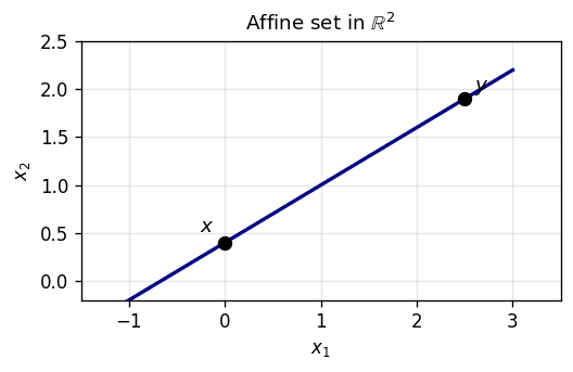
1.2 Affine Sets and Subspaces
Before defining convex sets, it is useful to introduce affine sets — the simpler, “flat” sets that form the backdrop for convex geometry. Affine sets allow unrestricted linear combinations, while convex sets only allow convex (weighted-average) combinations.
Definition 1.2.2 (Affine Subspace). An affine subspace is any nonempty affine set \(\emptyset \neq S \subseteq \mathbb{R}^n\).
Example 1.2.1. Let \(L\) be a linear subspace of \(\mathbb{R}^n\) and \(a \in \mathbb{R}^n\). Then \(L\), \(a + L\), \(\emptyset\), and \(\mathbb{R}^n\) are all examples of affine sets.
Unlike convex sets, affine sets are closed under arbitrary “linear interpolation-and-extrapolation”. Geometrically, an affine set is a “flat” — a point, line, plane, or hyperplane that extends infinitely in all directions along itself. Every linear subspace is affine (set \(\lambda = 0\) to see it contains \(0\)), and every translate \(a + L\) of a linear subspace \(L\) is affine. Conversely, every nonempty affine set \(A\) has a corresponding linear subspace \(L := A - A = \bigcup_{a \in A}(A - a)\).
The affine hull is the analogue of the linear span: just as the span is the smallest subspace containing a set, the affine hull is the smallest flat containing it. The dimension of a convex set is defined as the dimension of its affine hull, which captures the “intrinsic” dimension irrespective of the ambient space.
1.3 Convex Sets
With affine sets as our backdrop, we now define the central objects of this course. Convex sets are the natural setting for minimization because any local minimum of a convex function over a convex set is automatically a global minimum — a guarantee impossible in the general nonconvex setting.
The geometric picture is the key intuition: a set is convex if you can “see” every point from every other point without leaving the set. This “no hidden corners” property is precisely what makes convex optimization tractable.
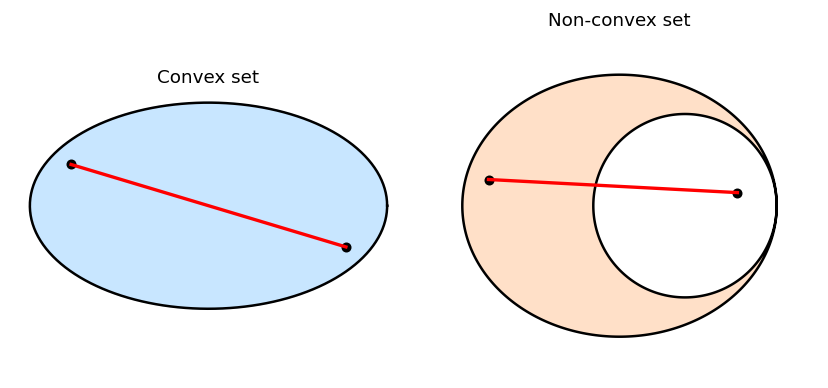
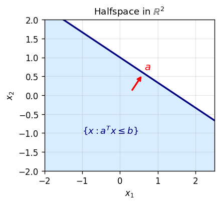
Example 1.3.1. \(\emptyset\), \(\mathbb{R}^n\), closed balls, affine sets, and halfspaces \(\{x : \langle a, x\rangle \leq b\}\) are all examples of convex sets.
One of the most important properties of convex sets is that they are stable under intersection — a fact that lets us build complex feasible regions by intersecting simple ones.
This theorem, whose proof is almost immediate, has enormous practical consequences: any optimization problem with multiple linear or convex constraints defines a convex feasible set, and the intersection theorem ensures we inherit all the geometric benefits of convexity.
1.4 Convex Combinations and the Convex Hull
The definition of convexity involves combinations of just two points. But iterating this, we can take weighted averages of arbitrarily many points — the resulting objects are convex combinations, and they characterize convex sets internally.
A convex combination is a generalized weighted average with nonnegative weights summing to one. Geometrically, it is a point strictly “inside” the simplex spanned by \(x_1, \ldots, x_m\).
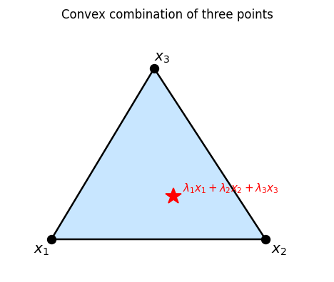
The inductive step re-normalizes the first \(m-1\) weights to sum to one, making the outer combination a two-point convex combination — a clean reduction to the base case. This argument also shows that convexity is equivalent to closure under finite convex combinations.
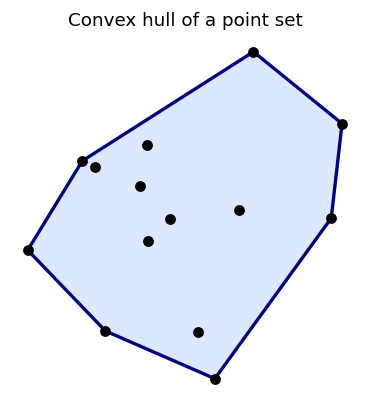
Theorem 1.4.2. \(\operatorname{conv} S\) consists of all convex combinations of elements of \(S\).
This gives a constructive description of the convex hull: any point in \(\operatorname{conv} S\) can be written as a finite convex combination of elements of \(S\).
The convex hull is the “tightest shrink-wrap” around a set — the smallest convex container. Its two equivalent descriptions (as an intersection and as a set of combinations) are both useful: the intersection description makes existence and closure properties immediate, while the combination description gives a constructive handle on the hull’s elements.
1.5 The Projection Theorem
The metric projection onto a convex set is a cornerstone of the theory, enabling both theoretical results (separation, supporting hyperplanes) and algorithms (projected gradient descent). The key question is: given a point \(x\) outside a convex set \(C\), is there a unique closest point in \(C\)?
The distance function measures how far a point is from the set. For closed sets, the infimum is attained; for convex sets, the attaining point is unique.
The projection operator is the geometric analogue of rounding to the nearest element: given any point, project it to the nearest feasible point in \(C\). Both closedness and convexity are needed for the projection to exist and be unique.
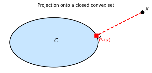
Without closedness, \(P_C(x)\) may not exist (no closest point reached). Without convexity, the projection may be non-unique.
Two lemmas prepare the proof of the Projection Theorem.
The Projection Theorem is one of the central results of this chapter: it not only guarantees existence and uniqueness of the projection, but gives a clean variational characterization that generalizes Fermat’s rule.
- For every \(x \in \mathbb{R}^n\), \(P_C(x)\) exists and is unique.
- For every \(x \in \mathbb{R}^n\) and \(p \in \mathbb{R}^n\), \[ p = P_C(x) \iff p \in C \text{ and } \forall y \in C,\ \langle y - p,\, x - p\rangle \leq 0. \]
Uniqueness follows by applying the same identity to two minimizers \(p, q\): it forces \(\|p - q\|^2 \leq 0\).
Characterization (ii): \(p = P_C(x)\) iff \(p\) minimizes \(\|x - \cdot\|\) over \(C\). For any \(y \in C\) and \(\alpha \in [0,1]\), the point \(\alpha y + (1-\alpha)p \in C\) gives \(\|x - p\|^2 \leq \|x - \alpha y - (1-\alpha)p\|^2\). Expanding and dividing by \(\alpha > 0\), then letting \(\alpha \to 0^+\) yields \(\langle y - p, x - p\rangle \leq 0\). \(\square\)
The existence proof uses the parallelogram identity to show that a minimizing sequence is Cauchy, then appeals to closedness; uniqueness uses the same identity to force any two minimizers to coincide. The variational characterization is derived by a first-order condition along segments from \(p\) towards any other feasible point.
That is, \(P_C(x) = x\) if \(x \in C\), and otherwise \(x\) is scaled to have norm \(\varepsilon\).
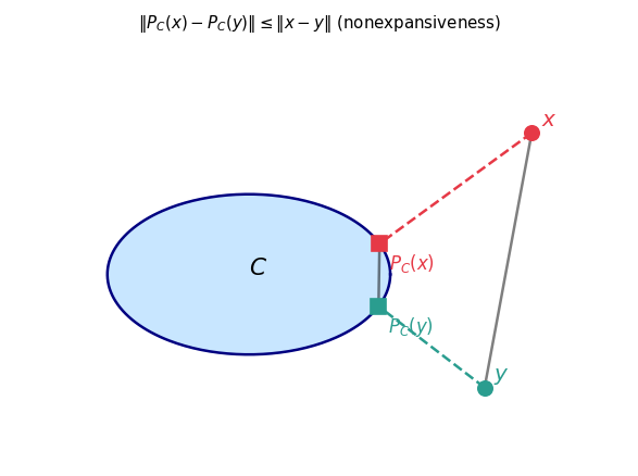
In particular, \(P_C\) is nonexpansive: \(\|P_C(x) - P_C(y)\| \leq \|x - y\|\).
1.6 Convex Set Operations
1.7 Topological Properties
- Interior: \(\operatorname{int} C = \{x : \exists \varepsilon > 0,\, x + \varepsilon B \subseteq C\}\) where \(B = \overline{B}(0;1)\).
- Closure: \(\overline{C} = \bigcap_{\varepsilon > 0} (C + \varepsilon B)\).
- Relative interior: \(\operatorname{ri} C = \{x \in \operatorname{aff} C : \exists \varepsilon > 0,\, (x + \varepsilon B) \cap \operatorname{aff} C \subseteq C\}\).
- Dimension of convex \(C\): \(\dim C := \dim(\operatorname{aff} C)\).
Proposition 1.7.1. Let \(C \subseteq \mathbb{R}^n\). If \(\operatorname{int} C \neq \emptyset\), then \(\operatorname{int} C = \operatorname{ri} C\).
When \(\operatorname{int} C \neq \emptyset\), we have \(\operatorname{ri} C = \operatorname{int} C\), since \(\operatorname{aff} C = \mathbb{R}^n\) in that case.
This is the key “line from interior to boundary stays in interior” property. An analogous result holds for the relative interior:
Theorem 1.7.3. Let \(C \subseteq \mathbb{R}^n\) be convex. For all \(x \in \operatorname{ri} C\) and \(y \in \overline{C}\), \([x,y) \subseteq \operatorname{ri} C\).
This implies:
- \(\overline{C}\) is convex.
- \(\operatorname{int} C\) is convex.
- If \(\operatorname{int} C \neq \emptyset\), then \(\operatorname{int} C = \operatorname{int} \overline{C}\) and \(\overline{C} = \overline{\operatorname{int} C}\).
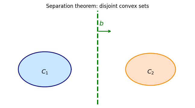
1.8 Separation Theorems
Separation theorems are among the most powerful tools in convex analysis. The geometric intuition is vivid: if two convex sets are disjoint, a hyperplane can be “slid between” them, separating them cleanly. This geometric fact has far-reaching analytic and algorithmic consequences — it is the foundation of duality theory, optimality conditions, and the theory of supporting hyperplanes.
Geometrically, separation says that the sets lie on opposite sides of the hyperplane \(\{x : \langle x, b\rangle = c\}\) for some \(c\). Strong separation means there is a positive gap between the sets, while weak separation allows them to touch the separating hyperplane from opposite sides.
The proof is elegantly short: the vector \(b = x - p\) pointing from the projection to \(x\) is exactly the separating direction, and the projection characterization gives the required inequality for free.
Corollary 1.8.1.1. Let \(C_1 \cap C_2 = \emptyset\) be nonempty subsets of \(\mathbb{R}^n\) such that \(C_1 - C_2\) is closed and convex. Then \(C_1\) and \(C_2\) are strongly separated.
Corollary 1.8.1.2. Let \(\emptyset \neq C_1, C_2 \subseteq \mathbb{R}^n\) be closed and convex such that \(C_1 \cap C_2 = \emptyset\) and \(C_2\) is bounded. Then \(C_1\) and \(C_2\) are strongly separated.
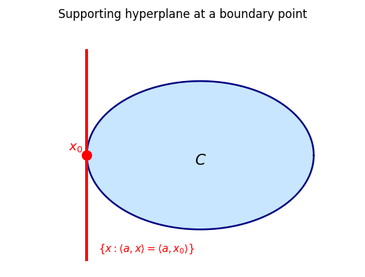
1.9 Cones, Tangent Cones, and Normal Cones
The separation theorems motivate a closer look at the local geometry of convex sets near their boundaries. The tangent cone and normal cone formalize the notion of “which directions are feasible” and “which gradients are inward-pointing” at a boundary point — concepts that are indispensable for optimality conditions.
- A set \(C\) is a cone if \(C = \mathbb{R}_{++} C\) (closed under positive scaling).
- The conical hull \(\operatorname{cone} C = \mathbb{R}_{++} C\) is the smallest cone containing \(C\).
- The closed conical hull \(\overline{\operatorname{cone}}(C)\) is the smallest closed cone containing \(C\).
- The tangent cone to \(C\) at \(x\) is \(T_C(x) = \overline{\operatorname{cone}(C - x)}\) for \(x \in C\), and \(\emptyset\) otherwise.
- The normal cone to \(C\) at \(x\) is \(N_C(x) = \{u : \sup_{c \in C}\langle c - x, u\rangle \leq 0\}\) for \(x \in C\), and \(\emptyset\) otherwise.
Proposition 1.9.1. Let \(C \subseteq \mathbb{R}^n\). The following hold:
- \(\operatorname{cone} C = \mathbb{R}_{++} C\).
- \(\operatorname{cone} C = \overline{\operatorname{cone}}(C)\) when \(C\) is a cone.
- \(\overline{\operatorname{cone}}(\operatorname{conv} C) = \operatorname{conv}(\operatorname{cone} C)\).
- \(\overline{\operatorname{cone}}(\operatorname{conv} C) = \operatorname{conv}(\operatorname{cone} C)\).
Lemma 1.9.2. Let \(0 \in C \subseteq \mathbb{R}^n\) be convex with \(\operatorname{int} C \neq \emptyset\). The following are equivalent:
- \(0 \in \operatorname{int} C\).
- \(\operatorname{cone} C = \mathbb{R}^n\).
- \(\overline{\operatorname{cone}}(C) = \mathbb{R}^n\).
Theorem 1.9.3. Let \(\emptyset \neq C \subseteq \mathbb{R}^n\) be closed and convex, and \(x \in \mathbb{R}^n\). Both \(N_C(x)\) and \(T_C(x)\) are closed convex cones.
Theorem 1.9.5. Let \(C \subseteq \mathbb{R}^n\) be convex with \(\operatorname{int} C \neq \emptyset\), and \(x \in C\). The following are equivalent:
- \(x \in \operatorname{int} C\).
- \(T_C(x) = \mathbb{R}^n\).
- \(N_C(x) = \{0\}\).
Tangent vectors point “into” or “along” the set from \(x\), while normal vectors point “outward” — making negative inner products with all feasible directions. Normal and tangent cones are dual to each other: \(u \in N_C(x)\) if and only if \(\langle u, t\rangle \leq 0\) for all \(t \in T_C(x)\). When \(x \in \operatorname{int} C\), \(T_C(x) = \mathbb{R}^n\) and \(N_C(x) = \{0\}\).
Chapter 2: Convex Functions
With the geometry of convex sets in place, we turn to convex functions — the functions that preserve the geometric structure of convex sets in their graphs. Chapter 2 develops the theory from the epigraph definition through the key analytic tools of subdifferentials, conjugates, and proximal operators.
2.1 Definitions and Basic Results
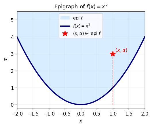
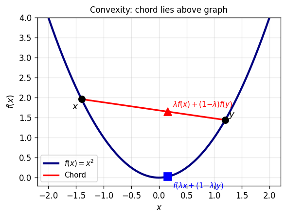
A convex function is one whose graph “curves upward” — the chord between any two points on the graph lies above the graph. The cleanest algebraic encoding of this is through the epigraph.
The epigraph is the set of points on or above the graph of \(f\). Demanding that this set is convex is equivalent to the classical Jensen inequality — the two formulations are interchangeable, but the epigraph viewpoint makes geometric arguments more transparent.
Definition 2.1.3 (Proper Function). We say \(f\) is proper if \(\operatorname{dom} f \neq \emptyset\) and \(f(\mathbb{R}^n) > -\infty\) (i.e., \(f\) never takes the value \(-\infty\)).
Properness is a mild regularity condition that rules out degenerate functions that are identically \(+\infty\) or take the value \(-\infty\). Most functions encountered in practice are proper, but the condition becomes important when taking conjugates and infimal convolutions.
Proposition 2.1.1. Let \(f : \mathbb{R}^n \to [-\infty, \infty]\) be convex. Then \(\operatorname{dom} f\) is convex.
Lower semicontinuity is the natural continuity condition for functions taking values in \([-\infty, \infty]\): it says that the function cannot “jump down” at a limit point.
The equivalence between the two definitions — one geometric (closed epigraph) and one analytic (liminf condition) — is one of the many places where the epigraph viewpoint unifies disparate characterizations.
We say \(f\) is l.s.c. if it is l.s.c. at every point.
Theorem 2.2.1. Let \(C \subseteq \mathbb{R}^m\). The following hold:
- \(C \neq \emptyset\) if and only if \(\delta_C\) is proper.
- \(C\) is convex if and only if \(\delta_C\) is convex.
- \(C\) is closed if and only if \(\delta_C\) is l.s.c.
Key examples: \(\delta_C\) (indicator function) is proper iff \(C \neq \emptyset\), convex iff \(C\) is convex, l.s.c. iff \(C\) is closed.
2.2 The Support Function
The support function is a canonical tool for encoding the geometry of a convex set as a function — it records, for each direction \(u\), the maximum extent of the set in that direction.
Proposition 2.3.1. Let \(\emptyset \neq C \subseteq \mathbb{R}^n\). Then \(\sigma_C\) is convex, l.s.c., and proper.
\(\sigma_C\) is always convex, l.s.c., and proper (it is a supremum of linear functions, which are affine hence convex). Crucially, \(\sigma_C\) determines \(C\) completely when \(C\) is closed and convex: the set \(C\) can be recovered as the intersection of the halfspaces \(\{\langle \cdot, u\rangle \leq \sigma_C(u)\}\) over all \(u\). This duality between convex sets and their support functions is the geometric heart of conjugate duality.
2.3 Further Notions of Convexity
For proper \(f\):
- Strict convexity: the Jensen inequality holds strictly for \(x \neq y\).
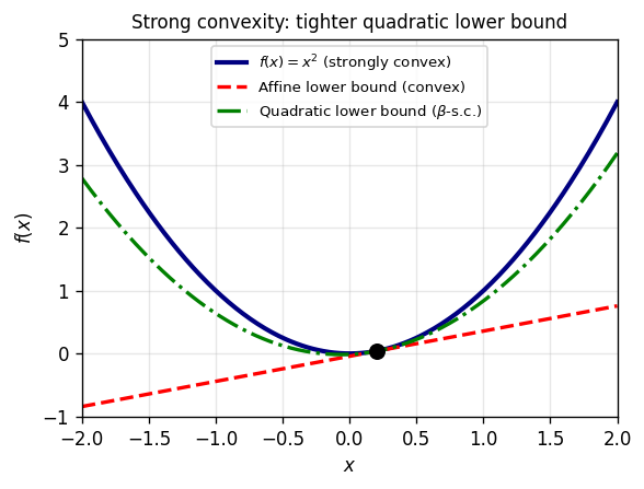
- \(\beta\)-strong convexity (constant \(\beta > 0\)): \(f(\lambda x + (1-\lambda)y) \leq \lambda f(x) + (1-\lambda)f(y) - \frac{\beta}{2}\lambda(1-\lambda)\|x-y\|^2\).
Strong \(\Rightarrow\) strict \(\Rightarrow\) convex. Equivalently, \(f\) is \(\beta\)-strongly convex iff \(f - \frac{\beta}{2}\|\cdot\|^2\) is convex.
A strongly convex, l.s.c., proper function has a unique minimizer.
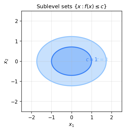
2.4 Further Notions of Convexity and Sublevel Sets
Every sublevel set of a convex function is convex. Conversely, convexity of all sublevel sets is strictly weaker than convexity of \(f\) (such functions are called quasiconvex).
Proposition 2.5.1. Let \(I\) be a finite index set and \((f_i)_{i \in I}\) a family of convex functions \(\mathbb{R}^m \to [-\infty, \infty]\). Then \(\sum_{i \in I} f_i\) is convex.
Proposition 2.5.2. Let \(f\) be convex, l.s.c., proper and \(\lambda > 0\). Then \(\lambda f\) is convex and l.s.c.
2.5 Minimizers
Definition 2.6.1 (Global Minimizer). Let \(f : \mathbb{R}^m \to (-\infty, \infty]\) be proper and \(x \in \mathbb{R}^m\). Then \(x\) is a (global) minimizer of \(f\) if \(f(x) = \min f(\mathbb{R}^m)\). We write \(\operatorname{argmin} f\) for the set of minimizers.
Definition 2.6.2 (Local Minimum). Let \(f : \mathbb{R}^m \to (-\infty, \infty]\) be proper. Then \(\bar{x}\) is a local minimum of \(f\) if there exists \(\delta > 0\) such that \(\|x - \bar{x}\| < \delta \Rightarrow f(\bar{x}) \leq f(x)\).
Proposition 2.6.2. Let \(f : \mathbb{R}^m \to (-\infty, \infty]\) be proper and convex, and \(C \subseteq \mathbb{R}^m\). If \(x\) minimizes \(f\) over \(C\) and \(x \in \operatorname{int} C\), then \(x\) is an (unconstrained) minimizer of \(f\).
Theorem 2.12.1. Let \(f : \mathbb{R}^m \to \mathbb{R}\) be proper, l.s.c., and let \(C \subseteq \mathbb{R}^m\) be compact with \(C \cap \operatorname{dom} f \neq \emptyset\). Then:
- \(f\) is bounded below over \(C\).
- \(f\) attains its minimal value over \(C\).
Definition 2.12.1 (Coercive Function). \(f : \mathbb{R}^m \to (-\infty, \infty]\) is coercive if \(\lim_{\|x\| \to \infty} f(x) = \infty\).
Definition 2.12.2 (Super Coercive). \(f : \mathbb{R}^m \to (-\infty, \infty]\) is super coercive if \(\lim_{\|x\| \to \infty} \frac{f(x)}{\|x\|} = \infty\).
Theorem 2.12.2. Let \(f : \mathbb{R}^m \to (-\infty, \infty]\) be proper, l.s.c., and coercive, and \(C \subseteq \mathbb{R}^m\) closed with \(C \cap \operatorname{dom} f \neq \emptyset\). Then \(f\) attains its minimal value over \(C\).
Existence via coercivity. \(f\) is coercive if \(f(x) \to \infty\) as \(\|x\| \to \infty\). If \(f\) is proper, l.s.c., and coercive, it attains its minimum over any nonempty closed set (reducing to minimization over a compact ball).
2.6 Conjugate Functions and Fenchel Duality
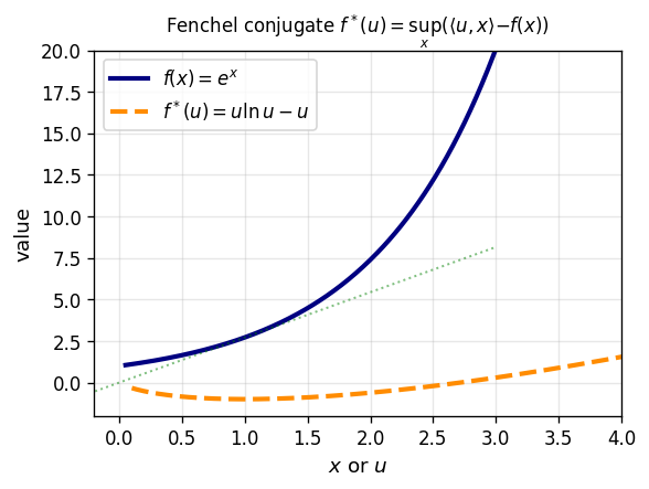
Duality is one of the most profound ideas in convex analysis: every convex minimization problem has a “mirror” dual problem, and the relationship between primal and dual reveals structural information about both. The Fenchel conjugate is the analytic mechanism that makes this duality precise.
Geometric interpretation. Given slope \(u\), the conjugate \(f^*(u)\) is the best intercept \(\alpha\) such that the affine function \(\langle u, \cdot\rangle - \alpha\) is a global lower bound on \(f\). In other words, \(f^*\) records the tightest affine underestimate of \(f\) in every direction — a “dual” description of \(f\) through its supporting hyperplanes. The convex, l.s.c. epigraph of \(f\) is recovered as the intersection of all supporting halfspaces from below.
Example 2.7.4. Let \(C \subseteq \mathbb{R}^m\). Then \(\delta_C^* = \sigma_C\). In other words, the conjugate of the indicator function of a set is its support function.
Key examples:
- \(f(x) = |x|^p/p\) \(\Rightarrow\) \(f^*(u) = |u|^q/q\) where \(1/p + 1/q = 1\).
- \(f(x) = e^x\) \(\Rightarrow\) \(f^*(u) = u\ln u - u\) for \(u > 0\), \(0\) for \(u = 0\), \(\infty\) for \(u < 0\).
- \(f = \delta_C\) \(\Rightarrow\) \(f^* = \sigma_C\) (indicator’s conjugate is the support function).
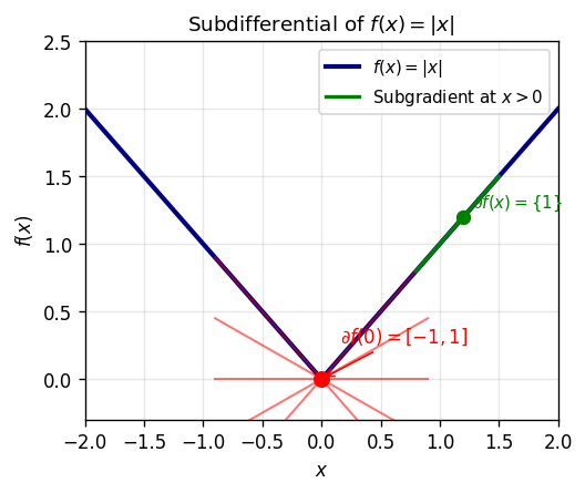
2.7 The Subdifferential Operator
For non-smooth convex functions, the gradient is replaced by the subdifferential. While a smooth function has a unique tangent plane at each point (its gradient), a non-smooth function like \(|x|\) can have many supporting hyperplanes at a kink — the subdifferential collects all of them.
Geometrically, \(u\) is a subgradient at \(x\) if the affine function \(f(x) + \langle u, \cdot - x\rangle\) is a global supporting hyperplane to the graph of \(f\) from below. At smooth points, \(\partial f(x) = \{\nabla f(x)\}\) is a singleton; at kinks, it is an interval or convex set recording all supporting hyperplanes.
Lemma 2.8.3. Let \(f : \mathbb{R}^m \to (-\infty, \infty]\) be proper. Then \(\operatorname{dom} \partial f \subseteq \operatorname{dom} f\).
Proposition 2.8.4. Let \(\emptyset \neq C \subseteq \mathbb{R}^m\) be closed and convex. Then \(\partial \delta_C(x) = N_C(x)\).
Connection to indicator functions. \(\partial \delta_C(x) = N_C(x)\) for closed convex \(C\).
Fermat’s rule for non-smooth functions is the fundamental optimality condition that generalizes \(\nabla f(x^*) = 0\) to the non-smooth setting.
This is the non-smooth analogue of the first-order condition: \(x^*\) minimizes \(f\) if and only if \(0\) is a subgradient of \(f\) at \(x^*\) — meaning the zero affine function is a global underestimate of \(f - f(x^*)\). The elegance of this condition is that it unifies smooth and non-smooth optimality in a single framework.
When \(f\) is differentiable at \(x\), \(f'(x; d) = \langle \nabla f(x), d\rangle\).
Theorem 2.10.2. Let \(f : \mathbb{R}^m \to (-\infty, \infty]\) be convex and proper, and \(x \in \operatorname{dom} f\). Then \(u \in \partial f(x)\) if and only if \(f'(x; d) \geq \langle u, d\rangle\) for all \(d \in \mathbb{R}^m\).
Lemma 2.10.4. Let \(\varphi : \mathbb{R} \to (-\infty, \infty]\) be proper and differentiable on a nonempty interval \(I \subseteq \operatorname{dom} \varphi\). If \(\varphi'\) is increasing on \(I\), then \(\varphi\) is convex on \(I\).
Proposition 2.10.5. Let \(f : \mathbb{R}^m \to (-\infty, \infty]\) be proper, with \(\operatorname{dom} f\) open and convex, and \(f\) differentiable on \(\operatorname{dom} f\). The following are equivalent:
- \(f\) is convex.
- For all \(x, y \in \operatorname{dom} f\): \(f(x) \geq f(y) + \langle \nabla f(y), x - y\rangle\).
- For all \(x, y \in \operatorname{dom} f\): \(\langle \nabla f(x) - \nabla f(y), x - y\rangle \geq 0\).
Example 2.10.6. Let \(A\) be an \(m \times m\) matrix and \(f(x) = \langle x, Ax\rangle\). Then \(\nabla f(x) = (A + A^T)x\) and \(f\) is convex if and only if \(A + A^T\) is positive semidefinite.
always exists, and \(u \in \partial f(x)\) iff \(f'(x; d) \geq \langle u, d\rangle\) for all \(d\).
2.8 Calculus of Subdifferentials
The fundamental question: when does \(\partial(f + g)(x) = \partial f(x) + \partial g(x)\)?
Definition 2.9.1 (Properly Separated). Let \(\emptyset \neq C_1, C_2 \subseteq \mathbb{R}^m\). Then \(C_1, C_2\) are properly separated if they are separated (i.e., \(\sup_{c_1 \in C_1}\langle b, c_1\rangle \leq \inf_{c_2 \in C_2}\langle b, c_2\rangle\) for some \(b \neq 0\)) and \(C_1 \cup C_2\) is not fully contained in the separating hyperplane.
Proposition 2.9.2. Let \(\emptyset \neq C_1, C_2 \subseteq \mathbb{R}^m\) be convex. Then \(C_1, C_2\) are properly separated if and only if \(\operatorname{ri} C_1 \cap \operatorname{ri} C_2 = \emptyset\).
Moreover, \(\operatorname{ri}(\lambda C) = \lambda(\operatorname{ri} C)\) for all \(\lambda \in \mathbb{R}\).
Proposition 2.9.4. Let \(C_1 \subseteq \mathbb{R}^m\) and \(C_2 \subseteq \mathbb{R}^p\) be convex. Then \(\operatorname{ri}(C_1 \oplus C_2) = \operatorname{ri} C_1 \oplus \operatorname{ri} C_2\).
The proof uses proper separation of epigraphs in \(\mathbb{R}^{n+2}\) and the normal cone sum formula \(N_{C_1 \cap C_2}(x) = N_{C_1}(x) + N_{C_2}(x)\) when \(\operatorname{ri} C_1 \cap \operatorname{ri} C_2 \neq \emptyset\).
\[ \bar{x} \text{ solves } (P) \iff 0 \in \partial f(\bar{x}) + N_C(\bar{x}) \iff \partial f(\bar{x}) \cap (-N_C(\bar{x})) \neq \emptyset. \]Example 2.9.8. Let \(d \in \mathbb{R}^m\) and \(\emptyset \neq C \subseteq \mathbb{R}^m\) be closed and convex. Consider \(\min_{x \in C} \langle d, x\rangle\). Then \(\bar{x}\) solves this problem if and only if \(-d \in N_C(\bar{x})\).
This is a powerful symmetry used in algorithmic duality.
2.9 Lipschitz Continuity and Second-Order Conditions
For twice continuously differentiable \(f\): \(\nabla f\) is \(L\)-Lipschitz iff \(\|\nabla^2 f(x)\| \leq L\) everywhere; for PSD Hessians, this equals \(\lambda_{\max}(\nabla^2 f(x)) \leq L\).
Example 2.13.1. Let \(f : \mathbb{R}^m \to \mathbb{R}\) be given by \(f(x) = \frac{1}{2}\langle x, Ax\rangle + \langle b, x\rangle + c\) where \(A \succeq 0\), \(b \in \mathbb{R}^m\), \(c \in \mathbb{R}\). Then:
- \(\nabla f(x) = Ax + b\) for all \(x\).
- \(\nabla f\) is Lipschitz with constant \(\|A\|\) (the operator norm of \(A\)).
Example 2.13.2. Let \(\emptyset \neq C \subseteq \mathbb{R}^m\) be closed and convex. Then \(P_C\) is Lipschitz continuous with constant \(1\).
Theorem 2.13.7 (Second Order Characterization). Let \(f : \mathbb{R}^m \to \mathbb{R}\) be twice continuously differentiable on \(\mathbb{R}^m\) and \(L \geq 0\). The following are equivalent:
- \(\nabla f\) is \(L\)-Lipschitz.
- For all \(x \in \mathbb{R}^m\), \(\|\nabla^2 f(x)\| \leq L\) (operator norm).
where \(\lambda_i\) are the eigenvalues of \(A\).
Proposition 2.13.9. A twice continuously differentiable function \(f : \mathbb{R}^m \to \mathbb{R}\) is convex if and only if \(\nabla^2 f(x)\) is positive semidefinite for all \(x\).
Corollary 2.13.9.1. Let \(f : \mathbb{R}^m \to \mathbb{R}\) be convex and twice continuously differentiable, and \(L \geq 0\). Then \(\nabla f\) is \(L\)-Lipschitz if and only if \(\lambda_{\max}(\nabla^2 f(x)) \leq L\) for all \(x \in \mathbb{R}^m\).
Example 2.13.10. Let \(f : \mathbb{R}^m \to \mathbb{R}\) be given by \(f(x) = \sqrt{1 + \|x\|^2}\). Then:
- \(f\) is convex.
- \(\nabla f\) is \(1\)-Lipschitz.
Proposition 2.13.11. Let \(\beta > 0\). Then \(f : \mathbb{R}^m \to (-\infty, \infty]\) is \(\beta\)-strongly convex if and only if \(f - \frac{\beta}{2}\|\cdot\|^2\) is convex.
Proposition 2.13.12. Let \(f, g : \mathbb{R}^m \to (-\infty, \infty]\) and \(\beta > 0\). Suppose \(f\) is \(\beta\)-strongly convex and \(g\) is convex. Then \(f + g\) is \(\beta\)-strongly convex.
Proposition 2.13.13. Let \(f : \mathbb{R}^m \to (-\infty, \infty]\) be strongly convex, l.s.c., and proper. Then \(f\) has a unique minimizer.
2.10 The Proximal Operator
The proximal operator is the workhorse of modern first-order algorithms, generalizing projection to arbitrary convex functions. Where the projection operator finds the nearest point in a convex set, the proximal operator finds the nearest point that also has a small function value — a regularized nearest-point problem.
The proximal operator interpolates between the identity map (when \(f = 0\)) and the projection onto a convex set (when \(f = \delta_C\)). For a general convex function, it moves from \(x\) towards the minimizer of \(f\), with the quadratic term preventing too large a step.
This tells us that the proximal operator is a well-defined function — not just a set-valued map — because the \(\frac{1}{2}\|u-x\|^2\) term breaks ties by selecting the unique closest minimizer.
Equivalently, \(x - p \in \partial f(p)\), i.e., \(p = (\operatorname{Id} + \partial f)^{-1}(x)\).
Example 2.14.2. For \(\emptyset \neq C \subseteq \mathbb{R}^m\) closed and convex, \(\operatorname{Prox}_{\delta_C} = P_C\). That is, the proximal operator of the indicator function is the projection.
Example 2.14.6. Convexity is crucial for the proximal operator to be well-defined (singleton-valued). For a non-convex function such as \(h(x) = 0\) for \(x \neq 0\) and \(h(0) = -\lambda\), the proximal operator can be empty-valued.
and for \(x = 0\), \(\operatorname{Prox}_f(0) = \{u \in \mathbb{R}^m : \|u\| = \operatorname{Prox}_g(0)\}\).
equivalently \(x - p \in \partial f(p)\), i.e., \(p = (\operatorname{Id} + \partial f)^{-1}(x)\).
Key examples:
- \(f = \delta_C\): \(\operatorname{Prox}_{\delta_C} = P_C\) (projection is the special case).
- \(f(x) = |x|\): soft-thresholding \(\operatorname{Prox}_f(x) = \operatorname{sign}(x)(|x|-1)_+\).
- \(f(x) = \lambda|x|\): \(\operatorname{Prox}_f(x) = \operatorname{sign}(x)(|x|-\lambda)_+ =: S_\lambda(x)\).
2.11 Nonexpansive and Averaged Operators
The convergence theory for iterative algorithms rests on the notion of nonexpansive operators — maps that never increase distances. Understanding which operators are nonexpansive (or the stronger “firmly nonexpansive”) is the key to proving convergence.
- \(T : \mathbb{R}^n \to \mathbb{R}^n\) is nonexpansive if \(\|Tx - Ty\| \leq \|x - y\|\).
- \(T\) is firmly nonexpansive (f.n.e.) if \(\|Tx - Ty\|^2 + \|(I-T)x - (I-T)y\|^2 \leq \|x - y\|^2\), equivalently \(\|Tx - Ty\|^2 \leq \langle x - y, Tx - Ty\rangle\).
- \(T\) is \(\alpha\)-averaged (\(\alpha \in (0,1)\)) if \(T = (1-\alpha)\operatorname{Id} + \alpha N\) for some nonexpansive \(N\).
Proposition 2.15.1. Let \(T : \mathbb{R}^m \to \mathbb{R}^m\). The following are equivalent:
- \(T\) is firmly nonexpansive.
- \(\operatorname{Id} - T\) is firmly nonexpansive.
- \(2T - \operatorname{Id}\) is nonexpansive.
- For all \(x, y\): \(\|Tx - Ty\|^2 \leq \langle x - y, Tx - Ty\rangle\).
- For all \(x, y\): \(\langle Tx - Ty, (\operatorname{Id}-T)x - (\operatorname{Id}-T)y\rangle \geq 0\).
Proposition 2.15.2. Let \(T : \mathbb{R}^m \to \mathbb{R}^m\) be linear. The following are equivalent:
- \(T\) is f.n.e.
- \(\|2T - \operatorname{Id}\| \leq 1\).
- For all \(x\): \(\|Tx\|^2 \leq \langle x, Tx\rangle\).
- For all \(x\): \(\langle Tx, x - Tx\rangle \geq 0\).
Example 2.15.3. Let \(\emptyset \neq C \subseteq \mathbb{R}^m\) be convex and closed. Then \(P_C\) is firmly nonexpansive: for all \(x, y \in \mathbb{R}^m\), \(\|P_C(x) - P_C(y)\|^2 \leq \langle P_C(x) - P_C(y), x - y\rangle\).
Example 2.15.4. \(T = -\frac{1}{2}\operatorname{Id}\) is averaged (specifically, \(\frac{3}{4}\)-averaged via \(T = \frac{1}{4}\operatorname{Id} + \frac{3}{4}(-\operatorname{Id})\)) but NOT firmly nonexpansive.
Example 2.15.5. \(T = -\operatorname{Id}\) is nonexpansive but NOT averaged. Indeed, writing \(-\operatorname{Id} = (1-\alpha)\operatorname{Id} + \alpha N\) for nonexpansive \(N\) would require \(\|N\| = \frac{2-\alpha}{\alpha} > 1\) for any \(\alpha \in (0,1)\).
Proposition 2.15.6. Let \(T : \mathbb{R}^m \to \mathbb{R}^m\) be nonexpansive. Then \(T\) is continuous.
The hierarchy firm nonexpansive \(\Rightarrow\) averaged \(\Rightarrow\) nonexpansive is strict at each step. Firm nonexpansiveness is the “just right” condition for convergence: strong enough to guarantee convergence to a fixed point, but weak enough to include the proximal operator and the projection. Firm nonexpansiveness \(\Leftrightarrow\) \(\frac{1}{2}\)-averaged \(\Leftrightarrow\) \(2T - \operatorname{Id}\) is nonexpansive.
2.12 Féjer Monotonicity and Convergence
Here is one of the most beautiful ideas in iterative optimization: what if an algorithm does not know where the solution is, yet we can still prove it is getting closer?
This is exactly what Féjer monotonicity captures. Imagine you are lost in a forest, and you know there is a village somewhere — but you do not know where. You cannot tell whether you are converging toward it. Féjer monotonicity is the remarkable condition that, for every possible position the village might be, your distance to that position is non-increasing at every step. You are not searching randomly — you are monotonically approaching every candidate solution simultaneously, without knowing which one you will land at.
This notion is far stronger than it might first appear. Consider the geometry: if a sequence \((x_n)\) satisfies \(\|x_{n+1} - c\| \leq \|x_n - c\|\) for every \(c\) in a nonempty target set \(C\), then the entire sequence is trapped in the closed ball of radius \(\|x_0 - c\|\) around each target point \(c\). These constraints, taken together, force the sequence to be bounded. Moreover, since the distance from \(x_n\) to any fixed \(c \in C\) is monotone and bounded below by zero, it must converge — we know the limit of the distance even without knowing the limit of the iterates themselves.
The conceptual leap comes next: proving that an algorithm produces a Féjer monotone sequence reduces the entire convergence problem to showing that cluster points land in \(C\). Once you establish that, the convergence theorem does the rest. This is why Féjer monotonicity appears again and again as the keystone in convergence proofs for proximal gradient, Douglas–Rachford, and subgradient methods alike.
Example 2.16.1. Suppose \(\operatorname{Fix} T \neq \emptyset\) for some nonexpansive \(T : \mathbb{R}^m \to \mathbb{R}^m\). For any \(x_0 \in \mathbb{R}^m\), the sequence defined recursively by \(x_n := T(x_{n-1})\) is Féjer monotone with respect to \(\operatorname{Fix} T\).
Proposition 2.16.2. Let \(\emptyset \neq C \subseteq \mathbb{R}^m\) and \((x_n)_{n \geq 0}\) be a Féjer monotone sequence with respect to \(C\). The following hold:
- \((x_n)\) is bounded.
- For every \(c \in C\), \((\|x_n - c\|)_{n \geq 0}\) converges.
- \((d_C(x_n))_{n \geq 0}\) is decreasing and converges.
Féjer-monotone sequences are automatically bounded (since all points stay in the closed ball around the starting point) and have converging distance sequences (since \(d(x_n, C)\) is monotone and bounded below by 0).
These three consequences are not merely technical bookkeeping — they embody a profound structural fact: Féjer monotone sequences are “well-behaved” in the strongest sense. They cannot escape to infinity. They cannot oscillate wildly in distance to the target set. The only remaining question is whether the sequence converges as opposed to having multiple cluster points scattered across \(C\). The next two results close this gap completely.
Proposition 2.16.3. A bounded sequence \((x_n)_{n \in \mathbb{N}}\) in \(\mathbb{R}^m\) converges if and only if it has a unique cluster point.
Lemma 2.16.4. Let \((x_n)_{n \in \mathbb{N}}\) be a sequence in \(\mathbb{R}^m\) and \(\emptyset \neq C \subseteq \mathbb{R}^m\) such that for all \(c \in C\), the sequence \((\|x_n - c\|)_{n \in \mathbb{N}}\) converges, and every cluster point of \((x_n)\) lies in \(C\). Then \((x_n)\) converges to a point in \(C\).
The proof is a two-line argument: because the sequence is Féjer monotone, distances \(\|x_n - c\|\) converge for every \(c \in C$; if there were two cluster points \(x, y \in C\), then \(\|x_n - x\|\) and \(\|x_n - y\|\) must converge to the same limit along two subsequences, forcing \(x = y\) by the triangle inequality. The uniqueness of the cluster point, combined with boundedness, gives full convergence.
This theorem is the engine behind virtually every convergence proof in this chapter. The recipe is always the same: (1) establish Féjer monotonicity, (2) show cluster points lie in the target set, (3) conclude convergence. Theorem 2.16.6 instantiates this recipe for averaged operators — the broadest class of maps for which fixed-point iterations provably converge.
- \((x_n)\) is Féjer monotone w.r.t. \(\operatorname{Fix} T\).
- \(Tx_n - x_n \to 0\).
- \(x_n\) converges to a point in \(\operatorname{Fix} T\).
Corollary 2.16.6.1. Let \(T : \mathbb{R}^m \to \mathbb{R}^m\) be firmly nonexpansive with \(\operatorname{Fix} T \neq \emptyset\). Put \(x_0 \in \mathbb{R}^m\) and define \(x_{n+1} := Tx_n\) recursively. Then there exists \(\bar{x} \in \operatorname{Fix} T\) such that \(x_n \to \bar{x}\).
Corollary 2.16.7.1. Let \(f : \mathbb{R}^m \to (-\infty, \infty]\) be convex, l.s.c., and proper with \(\operatorname{argmin} f \neq \emptyset\). Let \(x_0 \in \mathbb{R}^m\) with \(x_{n+1} := \operatorname{Prox}_f(x_n)\). Then there exists \(\bar{x} \in \operatorname{argmin} f\) such that \(x_n \to \bar{x}\).
What does this mean practically? If you have a convex function with a nonempty solution set and you simply iterate the proximal operator — a fixed-point iteration that is “nothing but” moving toward the nearest minimizer — you are guaranteed to converge. Note there is no step-size tuning, no line search, no learning rate to hand-select. The firmly nonexpansive structure of \(\operatorname{Prox}_f\) makes convergence automatic. This is the power of working in the right abstract framework: the Féjer–averaged operator theory simultaneously covers gradient descent (for smooth functions), the proximal point algorithm, projected subgradient, and all the splitting algorithms we encounter in Chapter 5, through a single convergence engine.
Composition of averaged operators. If \(T_1\) is \(\alpha_1\)-averaged and \(T_2\) is \(\alpha_2\)-averaged, then \(T_1 T_2\) is \(\alpha\)-averaged with \(\alpha = \frac{\alpha_1 + \alpha_2 - 2\alpha_1\alpha_2}{1 - \alpha_1\alpha_2}\).
Proposition 2.17.1. Let \(T : \mathbb{R}^m \to \mathbb{R}^m\) be nonexpansive and \(\alpha \in (0,1)\). The following are equivalent:
- \(T\) is \(\alpha\)-averaged.
- \(\left(1 - \frac{1}{\alpha}\right)\operatorname{Id} + \frac{1}{\alpha}T\) is nonexpansive.
- For each \(x, y \in \mathbb{R}^m\): \(\|Tx - Ty\|^2 \leq \|x - y\|^2 - \frac{1-\alpha}{\alpha}\|({\operatorname{Id}} - T)x - (\operatorname{Id} - T)y\|^2\).
Chapter 3: Conjugate Functions and Duality
The conjugate function, introduced in Chapter 2 as a tool for studying individual functions, now takes center stage as the mechanism for constructing dual problems. Chapter 3 shows that every convex minimization problem has a “dual” formulation — obtained by conjugating the objective and constraints — and that strong duality (primal equals dual optimal value) holds under mild regularity conditions.
3.1 Conjugacy and the Biconjugate Theorem
We have already introduced the Fenchel conjugate \(f^*\) in Chapter 2. Let us now collect the key conjugacy results, culminating in the biconjugate theorem — which says that the double conjugate of a convex l.s.c. function recovers the original function exactly.
Proposition 2.11.1. Let \(f, g : \mathbb{R}^m \to [-\infty, \infty]\). Then:
- \(f^{**} := (f^*)^* \leq f\) always.
- \(f \leq g \Rightarrow f^* \geq g^*\) and \(f^{**} \leq g^{**}\) (conjugation reverses order).
Proposition 2.11.4. Let \(f : \mathbb{R}^m \to (-\infty, \infty]\) be convex and proper. If \(\partial f(x) \neq \emptyset\) for some \(x\), then \(f^{**}(x) = f(x)\).
Proposition 2.11.5. Let \(f : \mathbb{R}^m \to (-\infty, \infty]\) be proper. Then \(f\) is convex and l.s.c. if and only if \(f = f^{**}\). In this case, \(f^*\) is also proper.
Corollary 2.11.5.1. Let \(f : \mathbb{R}^m \to (-\infty, \infty]\) be convex, l.s.c., and proper. Then:
- \(f^*\) is convex, l.s.c., and proper.
- \(f^{**} = f\).
- \(f^{**} \leq f\) always.
- \(f \leq g \Rightarrow f^* \geq g^*\) (conjugation reverses order).
- If \(f\) is convex and l.s.c., \(f^{**} = f\) (the biconjugate theorem).
- For convex, l.s.c., proper \(f\): \(u \in \partial f(x) \Leftrightarrow f(x) + f^*(u) = \langle x, u\rangle \Leftrightarrow x \in \partial f^*(u)\).
3.2 Fenchel Duality
Duality is a lens that transforms a difficult minimization problem into a different — sometimes easier — one while preserving the optimal value. The Fenchel duality framework is the most elegant instantiation of this idea for convex programs: it produces a dual problem whose optimal value equals the primal’s under a mild regularity condition called constraint qualification.
The intuition is variational. For the sum \(f + g\), the conjugate of the sum is in general not the sum of conjugates — but by introducing an auxiliary variable \(z\) and forcing \(x = z\) via a Lagrange multiplier, we decouple \(f\) and \(g\) and can take conjugates independently. The resulting dual problem is expressed entirely in terms of \(f^*\) and \(g^*\), so the two functions appear in “dual form.” Weak duality — that the dual optimal value is always a lower bound on the primal — follows immediately from the Fenchel–Young inequality. Strong duality, that the two are equal, requires the regularity condition \(\operatorname{ri}\operatorname{dom} f \cap \operatorname{ri}\operatorname{dom} g \neq \emptyset\), which ensures the Lagrangian is well-behaved.
\[ L(x, z; y) = f(x) + g(z) + \langle y, z - x\rangle. \]The dual function is \(d(u) = \inf_{x,z} L(x,z;u) = -f^*(u) - g^*(-u)\). Setting \(p = \inf(f + g)\) and \(d^* = \inf(f^* + g^*(\cdot \circ (-\operatorname{Id})))\), weak duality gives \(p \geq -d^*\).
3.3 Fenchel–Rockafellar Duality
The Fenchel–Rockafellar theorem is the canonical strong duality result for convex programs with a linear coupling \(Ax\). It generalizes Lagrangian duality, LP duality, and semidefinite duality as special cases, and is the theoretical foundation underlying all the primal-dual algorithms in Chapter 5.
The key idea is that the linear map \(A\) passes through the conjugation operation cleanly: the conjugate of \(x \mapsto g(Ax)\) is \(u \mapsto g^*(A^{-T}u)\) — or more precisely, for the adjoint \(A^T\), the conjugate becomes \(g^* \circ (\cdot)^T\) evaluated at the dual variable. This is why the dual problem involves \(f^*(-A^T y)\) and \(g^*(y)\): the linear map in the primal is “absorbed” into the conjugate, and the dual variable \(y\) plays the role of a Lagrange multiplier for the constraint \(Ax = z\). Plugging in specific choices of \(f\), \(g\), and \(A\) recovers the LP dual, the semidefinite dual, and the dual of the LASSO problem respectively.
\[ (D): \quad \min_{y \in \mathbb{R}^m} f^*(-A^T y) + g^*(y). \]Strong duality holds (primal = dual optimal values) under regularity conditions such as \(\operatorname{ri}(\operatorname{dom} f) \cap A^{-1}(\operatorname{ri}(\operatorname{dom} g)) \neq \emptyset\).
Chapter 4: Optimality Conditions and Subdifferentials
With the theory of subdifferentials and duality established, Chapter 4 translates these tools into concrete optimality conditions for constrained problems. The subdifferential sum rule, the KKT conditions, and the normal cone characterization are all facets of the same underlying principle: at a minimizer, no feasible descent direction exists.
4.1 Optimality for Constrained Problems
Consider the constrained problem \(\min_{x \in C} f(x)\) with \(f\) convex, l.s.c., proper and \(C\) closed convex. Encoding the constraint as \(\min f + \delta_C\) and applying the sum rule brings us to a clean characterization of optimality in terms of normal cones.
4.2 Smooth + Non-smooth Optimality
- If \(f\) is differentiable at a local minimum \(x^*\), then \(-\nabla f(x^*) \in \partial g(x^*)\).
- If additionally \(f\) is convex, then \(x^*\) is global iff \(-\nabla f(x^*) \in \partial g(x^*)\).
4.3 KKT Conditions
The KKT conditions are the central tool of constrained optimization theory: they give necessary and, under convexity, sufficient conditions for a point to solve a constrained minimization problem. Their power lies in converting a constrained problem into an unconstrained system of equations and inequalities.
The Fritz-John conditions follow from a key lemma. Setting \(F(x) := \max\{f(x) - \mu, g_1(x), \ldots, g_n(x)\}\) where \(\mu\) is the optimal value:
Lemma 3.1.2. For all \(x \in \mathbb{R}^m\), \(F(x) \geq 0\). Moreover, the solutions of \((P)\) are precisely the minimizers of \(F\), i.e., \(\{x : F(x) = 0\}\).
The Fritz-John conditions are a weaker form that does not guarantee \(\alpha_0 > 0\): the objective function might be multiplied by zero, yielding degenerate conditions. Slater’s constraint qualification rules this out.
The sufficiency theorem completes the picture: for convex problems, the KKT conditions are not just necessary but also sufficient for global optimality. This is in sharp contrast to the nonconvex setting, where KKT points can be saddle points or local maxima.
\[ \partial g(x) = \operatorname{conv}\Bigl\{\partial g_i(x) : i \in A(x)\Bigr\}, \quad A(x) = \{i : g_i(x) = g(x)\}. \]Chapter 5: Algorithms for Convex Optimization
Having developed the theory of convex functions, subdifferentials, and optimality conditions, we now turn to algorithms. Chapter 5 presents a hierarchy of methods — from simple gradient descent to accelerated proximal algorithms — each suited to a different setting determined by the smoothness and structure of the objective.
There is a beautiful connection between the theory we have built and the algorithms we are about to study. The subdifferential Fermat rule says \(x^*\) is optimal if and only if \(0 \in \partial f(x^*)\), or equivalently \(x^* \in (\operatorname{Id} + \partial f)^{-1}(x^*)\) — that is, \(x^*\) is a fixed point of the proximal operator. This reformulation turns every convex minimization problem into a fixed-point problem for a firmly nonexpansive operator, which is exactly the setting where the averaged-operator convergence theory from Section 2.12 applies. The algorithmic content of Chapter 5 is thus: how to construct, for each problem class, the right firmly nonexpansive operator whose fixed points are the solutions; then iterate.
5.1 Gradient Descent
For smooth unconstrained minimization \(\min_{x \in \mathbb{R}^n} f(x)\) with \(f\) differentiable, the simplest algorithm is gradient descent: repeatedly move in the direction of steepest descent.
Definition 3.2.1 (Descent Direction). Let \(f : \mathbb{R}^m \to (-\infty, \infty]\) be proper and \(x \in \operatorname{int}\operatorname{dom} f\). A vector \(d \in \mathbb{R}^m \setminus \{0\}\) is a descent direction of \(f\) at \(x\) if the directional derivative satisfies \(f'(x; d) < 0\).
If \(0 \neq \nabla f(x)\) exists, then \(-\nabla f(x)\) is a descent direction, since \(f'(x; -\nabla f(x)) = -\|\nabla f(x)\|^2 < 0\).
Algorithm. Initialize \(x_0\). Update \(x_{n+1} = x_n - t_n \nabla f(x_n)\) where \(t_n := \operatorname{argmin}_{t \geq 0} f(x_n - t\nabla f(x_n))\) (exact line search) or a fixed step size \(1/L\).
Theorem 3.2.1 (Peressini, Sullivan, Uhl). If \(f\) is strictly convex and coercive, then the gradient descent iterates \(x_n\) converge to the unique minimizer of \(f\).
For non-smooth functions, the negative subgradient is not necessarily a descent direction — a key pathology that motivates the subgradient method instead.
Then \(f\) is convex and differentiable on \(\mathbb{R}^2 \setminus ((-\infty, 0] \times \{0\})\), yet the steepest descent method starting from \(x_0 = (\gamma, 1)\) generates iterates \(x_n \to (0, 0)\), which is not a minimizer of \(f\) (in fact \(\operatorname{argmin} f = \emptyset\)).
5.2 Projected Subgradient Method
Gradient descent is elegant, but it relies on differentiability. The moment we encounter a non-smooth function — a sparsity-inducing \(\ell^1\) norm, a max-function, a distance function — the gradient does not exist at kinks, and the method cannot be applied. Worse, even when a subgradient exists, it is not guaranteed to be a descent direction: stepping in the direction \(-g\) for \(g \in \partial f(x)\) might increase the function value. The subgradient method accepts this pathology and instead proves convergence through a different mechanism entirely.
Now add a constraint: the feasible set \(C\) is closed and convex. After a subgradient step, the iterate \(x_n - t_n f'(x_n)\) will typically leave \(C\). The fix is immediate and geometrically natural — project back to \(C\). This is the geometric picture of the projected subgradient method: take a step in the (approximate) descent direction, then snap back to the feasible set by computing the nearest feasible point. The projection does not just enforce feasibility — by the projection theorem’s variational characterization, it also reduces distance to any point in \(C\), including any solution.
Crucially, unlike gradient descent, the subgradient step does not guarantee a decrease in function value at every iteration. The method may temporarily increase \(f\) on its way toward the solution set. What it does guarantee — and this is where Féjer monotonicity re-enters — is that the distance to the solution set is controlled. The key lemma below quantifies exactly the trade-off between progress toward the solution and the squared step size.
For \(\min_{x \in C} f(x)\) with \(C \subseteq \operatorname{int}\operatorname{dom} f\) and bounded subgradients \(\sup_{c \in C}\|\partial f(c)\| \leq L < \infty\):
Algorithm.
- Initialize \(x_0 \in C\).
- Pick subgradient \(f'(x_n) \in \partial f(x_n)\), step size \(t_n > 0\).
- Update \(x_{n+1} = P_C(x_n - t_n f'(x_n))\).
- \((x_n)\) is Féjer monotone w.r.t. \(S = \operatorname{argmin}_C f\).
- \(f(x_n) \to \mu\).
- \(\mu_n - \mu \leq \frac{L \cdot d_S(x_0)}{\sqrt{n+1}}\) where \(\mu_n = \min_{0 \leq k \leq n} f(x_k)\).
- \(x_n \to s \in S\).
Theorem 3.3.3 (Convergence of Projected Subgradient). Suppose \(x_n\) is generated by the projected subgradient method with Polyak’s rule. Then \(x_n \to s \in S\).
Let us pause to appreciate what Polyak’s step size accomplishes. In ordinary gradient descent, the step size \(1/L\) is chosen relative to the Lipschitz constant of the gradient — a smoothness parameter of \(f\). Polyak’s rule replaces this with an adaptive step size that depends on the current “suboptimality gap” \(f(x_n) - \mu\) and the current subgradient norm. When the iterate is far from optimal, the step is large; as the iterate approaches the solution, the step size shrinks proportionally. This adaptivity is precisely what enables Féjer monotonicity: substituting Polyak’s step into the key lemma causes the \(-2t_n(f(x_n) - \mu) + t_n^2 \|f'(x_n)\|^2\) term to collapse to \(-(f(x_n)-\mu)^2/\|f'(x_n)\|^2 \leq 0\). Every step contracts the distance to the solution set.
The \(O(1/\sqrt{n})\) rate in function value is slower than gradient descent’s \(O(1/n)\) — and this gap is provably unavoidable for non-smooth functions without additional structure. The price of generality is a slower convergence rate. This trade-off — smooth versus non-smooth, faster versus slower — motivates the hierarchy of algorithms we build next.
In particular, \(\sup\|\partial d_C(x)\| \leq 1\).
Lemma 3.3.5. Let \(f\) be convex, l.s.c., and proper. Fix \(\lambda > 0\). Then \(\partial(\lambda f) = \lambda \partial f\).
Convergence rate. The subgradient method achieves \(O(1/\sqrt{n})\) convergence in function value — significantly slower than gradient descent’s \(O(1/n)\) under smoothness.
Application: Convex Feasibility. To find a point in \(\bigcap_{i=1}^k S_i\), minimize \(f(x) = \max_i d_{S_i}(x)\). The projected subgradient step simplifies to: find the most violated constraint \(S_{\bar{\imath}}\) and project: \(x_{n+1} = P_{S_{\bar\imath}}(x_n)\) — this is the alternating projections algorithm.
5.3 Proximal Gradient Method (PGM)
Many important problems — including LASSO regression, basis pursuit, and sparse signal recovery — have a composite objective: a smooth term plus a non-smooth regularizer. The proximal gradient method handles this structure by applying gradient descent to the smooth part and the proximal operator to the non-smooth part in alternation.
To understand why the proximal gradient method is the right algorithm for this class of problems, we need to understand what the proximal operator is doing geometrically. Recall that \(\operatorname{Prox}_f(x)\) solves the problem \(\min_u \{f(u) + \frac{1}{2}\|u - x\|^2\}\). The quadratic term \(\frac{1}{2}\|u - x\|^2\) acts as a trust region: it penalizes moving too far from the current point \(x\), while the \(f(u)\) term pulls the result toward the minimizer of \(f\). The net effect is that \(\operatorname{Prox}_f(x)\) is the unique point that balances these two competing forces — it is as close as possible to \(x\) while also accounting for the shape of \(f\).
This is the Moreau envelope interpretation: the function \(e_f(x) := \min_u \{f(u) + \frac{1}{2}\|u - x\|^2\}\) is a smooth approximation to \(f$ — the "inf-convolution" of \(f\) with \(\frac{1}{2}\|\cdot\|^2\) — and \(\operatorname{Prox}_f(x)\) is the point at which this minimum is attained. As the parameter governing the proximal operator varies, the Moreau envelope interpolates between \(f\) itself (when the quadratic weight is very large, so we barely move) and the constant \(\min f\) (when the quadratic weight is very small, so we jump all the way to the minimizer). Crucially, the Moreau envelope is always differentiable, with gradient exactly \(x - \operatorname{Prox}_f(x)\) — the vector pointing from the proximal point back to \(x\).
The proximal gradient method exploits this structure for the composite problem \(F = f + g\). The smooth term \(f\) is handled by a gradient step — a linear approximation that is accurate within the Lipschitz ball. The non-smooth term \(g\) cannot be linearized, but its proximal operator handles it exactly. The two operations together define the update operator \(T = \operatorname{Prox}_{g/L}(\operatorname{Id} - \frac{1}{L}\nabla f)\), which is interpretable as: first take a gradient descent step for \(f\), then take a proximal step for \(g\).
For the composite problem \(\min_{x} F(x) := f(x) + g(x)\) where:
- \(f\) is convex, l.s.c., differentiable with \(L\)-Lipschitz gradient,
- \(g\) is convex, l.s.c., proper with \(\operatorname{dom} g \subseteq \operatorname{int}\operatorname{dom} f\).
Update operator. Define \(T = \operatorname{Prox}_{g/L}\bigl(\operatorname{Id} - \frac{1}{L}\nabla f\bigr)\). Fixed points of \(T\) are exactly the minimizers of \(F\):
where \(D_f(x, y) := f(x) - f(y) - \langle \nabla f(y), x - y\rangle\) is the Bregman distance.
Algorithm. \(x_{n+1} = Tx_n = \operatorname{Prox}_{g/L}\!\left(x_n - \frac{1}{L}\nabla f(x_n)\right)\).
- \((x_n)\) is Féjer monotone w.r.t. \(S\).
- \(0 \leq F(x_n) - \mu \leq \frac{L \cdot d_S^2(x_0)}{2n} \in O(1/n)\).
- \(x_n \to s \in S\).
The \(O(1/n)\) rate deserves careful attention. The bound \(F(x_n) - \mu \leq \frac{L \cdot d_S^2(x_0)}{2n}\) has a clean interpretation: the numerator \(L \cdot d_S^2(x_0)\) is a “problem-dependent constant” measuring the smoothness of \(f\) (via \(L\)) and the distance from the starting point to the solution set. The denominator grows linearly with the number of iterations, giving exactly \(O(1/n)\) convergence in function value. For practical purposes, to achieve \(\varepsilon\)-accuracy (i.e., \(F(x_n) - \mu \leq \varepsilon\)), PGM requires approximately \(n \approx \frac{L d_S^2(x_0)}{2\varepsilon}\) iterations.
This is strictly better than the subgradient method’s \(O(1/\sqrt{n})\) under the same assumptions — the smooth structure of \(f\) can be exploited through the gradient step, buying us an extra factor of \(\sqrt{n}\) in convergence speed. And the proximal operator handles the non-smooth part \(g\) exactly, without any approximation error. For LASSO, this translates directly: ISTA (PGM applied to \(\frac{1}{2}\|Ax - b\|^2 + \lambda\|x\|_1\)) converges at \(O(1/n)\) in the composite objective, requiring only soft-thresholding at each step.
Theorem 3.4.7 (Convergence of PGM). The iterates \(x_n\) converge to some solution in \(S := \operatorname{argmin}_{\mathbb{R}^m} F(x)\).
Proposition 3.4.8. The following hold:
- \(\frac{1}{L}\nabla f\) is firmly nonexpansive.
- \(\operatorname{Id} - \frac{1}{L}\nabla f\) is firmly nonexpansive.
- \(T = \operatorname{Prox}_{g/L}(\operatorname{Id} - \frac{1}{L}\nabla f)\) is \(\frac{2}{3}\)-averaged.
The update operator \(T\) is \(\frac{2}{3}\)-averaged (since \(\operatorname{Prox}_{g/L}\) and \(\operatorname{Id} - \frac{1}{L}\nabla f\) are both \(\frac{1}{2}\)-averaged, and the composition formula applies).
Corollary 3.4.9.1 (Classical Proximal Point Algorithm). Let \(g : \mathbb{R}^m \to (-\infty, \infty]\) be convex, l.s.c., and proper. Fix \(c > 0\). Assume \(S := \operatorname{argmin} g \neq \emptyset\). Update \(x_{n+1} := \operatorname{Prox}_{cg}(x_n)\). Then:
- \(g(x_n) \downarrow \mu := \min g(\mathbb{R}^m)\).
- \(0 \leq g(x_n) - \mu \leq \dfrac{d_S^2(x_0)}{2cn}\).
- \(x_n\) converges to a point in \(S\).
- \(\|x_{n-1} - x_n\| \leq \dfrac{\sqrt{2}\, d_S(x_0)}{\sqrt{n}}\).
Convergence: \(g(x_n) - \min g \leq \frac{d_S^2(x_0)}{2cn}\).
\[ \operatorname{Prox}_{g/L}(x) = \left(\operatorname{sign}(x_i)\max\!\left\{0, |x_i| - \frac{\lambda}{L}\right\}\right)_{i=1}^n, \]the soft-thresholding operator. Applied to \(\min \frac{1}{2}\|Ax - b\|^2 + \lambda\|x\|_1\) (LASSO), ISTA gives \(O(1/n)\) convergence.
where \(\lambda > 0\) and \(A \in \mathbb{R}^{n \times m}\). Set \(f(x) = \frac{1}{2}\|Ax-b\|_2^2\) and \(g(x) = \lambda\|x\|_1\). Then \(\nabla f(x) = A^T(Ax - b)\), which is \(L\)-Lipschitz for \(L := \lambda_{\max}(A^T A)\). The problem has a solution since \(f\) is coercive and continuous. Applying PGM (ISTA) gives \(O(1/n)\) convergence; applying FISTA gives \(O(1/n^2)\).
5.4 FISTA: Accelerated Proximal Gradient
The proximal gradient method achieves \(O(1/n)\) convergence, which is optimal for gradient-based methods without additional structure. But Nesterov’s remarkable insight is that by adding a carefully chosen “momentum” step — extrapolating beyond the current iterate — one can improve the convergence to \(O(1/n^2)\) without any additional oracle calls. FISTA (Fast Iterative Shrinkage–Thresholding Algorithm) implements this idea.
The key question is: where does the acceleration come from, and why does it feel like “cheating”? Intuitively, gradient descent and PGM are memoryless: the update at step \(n\) depends only on \(x_n\), discarding all history. Nesterov’s acceleration uses the previous iterate \(x_{n-1}\) as well, extrapolating in the direction of recent progress — a “momentum” that allows the method to overshoot slightly and explore further. The remarkable fact is that the momentum coefficients are determined by a specific algebraic sequence (the \(t_n\) sequence below) that precisely cancels the error terms in the telescoping convergence bound, upgrading \(O(1/n)\) to \(O(1/n^2)\). This is not a heuristic — it is an exact algebraic identity discovered by Nesterov in 1983, and FISTA (Beck–Teboulle, 2009) is its proximal instantiation.
\[ t_{n+1} = \frac{1 + \sqrt{1 + 4t_n^2}}{2}, \quad x_{n+1} = Ty_n, \quad y_{n+1} = x_{n+1} + \frac{t_n - 1}{t_{n+1}}(x_{n+1} - x_n). \]Proposition 3.5.1. The sequence \((t_n)_{n \in \mathbb{N}}\) satisfies \(t_n \geq \dfrac{n+2}{2}\).
This is a dramatic improvement over PGM’s \(O(1/n)\). For LASSO-type problems, FISTA is the method of choice.
The \(O(1/n^2)\) bound has a striking practical consequence. To achieve \(\varepsilon\)-accuracy in the composite objective, PGM requires approximately \(n = O(1/\varepsilon)\) iterations, while FISTA requires only \(n = O(1/\sqrt{\varepsilon})\) — a quadratic speedup for the same oracle cost per iteration. For LASSO with \(\varepsilon = 10^{-6}\), PGM might require one million iterations while FISTA requires only one thousand. This is not a constant-factor improvement — it is a qualitative change in the practical feasibility of the algorithm.
It is also worth noting that Nesterov proved this \(O(1/n^2)\) rate is optimal among all first-order methods for smooth convex minimization — no algorithm that uses only gradient evaluations can do better, even in principle. So FISTA achieves the information-theoretic lower bound with the same per-iteration cost as PGM. The price is that FISTA’s convergence analysis is more delicate: the iterates \(x_n\) themselves need not decrease monotonically in function value (unlike PGM), and the proof relies on a more sophisticated energy argument rather than simple Féjer monotonicity.
5.5 Douglas–Rachford Algorithm
When neither \(f\) nor \(g\) is smooth — for instance, in \(\ell^1 + \ell^2\) problems or feasibility problems with two constraint sets — neither gradient descent nor the proximal gradient method applies. The Douglas–Rachford algorithm is designed precisely for this fully non-smooth setting: it uses only the proximal operators of \(f\) and \(g\), not their gradients.
To build intuition, start with the special case where \(f = \delta_A\) and \(g = \delta_B\) for two closed convex sets \(A\) and \(B\). Then the problem \(\min \delta_A + \delta_B\) is simply the feasibility problem: find a point in \(A \cap B\). The proximal operators reduce to projections: \(\operatorname{Prox}_f = P_A\) and \(\operatorname{Prox}_g = P_B\). One might first try the alternating projections algorithm — project onto \(A\), then onto \(B\), repeat — and indeed this converges when \(A\) and \(B\) have nonempty intersection. But alternating projections can be slow when the sets are nearly parallel or nearly tangent, and it has no natural extension to general non-smooth optimization.
The Douglas–Rachford method makes a more subtle move. Instead of projecting, it uses reflections: \(R_f = 2P_A - \operatorname{Id}\) “reflects” a point through the set \(A\) — it maps a point to the mirror image of itself across the boundary of \(A\). The DR update \(T_{\mathrm{DR}} = \frac{1}{2}(\operatorname{Id} + R_g R_f)\) composes two such reflections and averages with the identity. This averaging is what converts the nonexpansive composition \(R_g R_f\) into a firmly nonexpansive operator, enabling the Féjer monotone convergence theory to apply.
Geometrically, one step of Douglas–Rachford does the following: from the current point \(x_n\), first reflect through \(A\) to get \(R_f(x_n)\), then reflect through \(B\) to get \(R_g R_f(x_n)\), then average with \(x_n\). The averaged point is \(x_{n+1}\). Critically, it is not the iterates \(x_n\) themselves that converge to the solution — it is the projections \(\operatorname{Prox}_f(x_n)\) that converge to a minimizer of \(f + g\). The iterates \(x_n\) live in an “auxiliary space” and converge to a fixed point of \(T_{\mathrm{DR}}\), which is not itself a solution. Extracting the solution requires one final proximal application.
This indirect structure is unusual but powerful: it allows Douglas–Rachford to handle fully non-smooth problems where no gradient information is available, relying entirely on the proximal structure of \(f\) and \(g\). The algorithm naturally extends beyond feasibility problems to general composite minimization, image reconstruction, compressed sensing, and machine learning problems with structured sparsity constraints.
For \(\min f(x) + g(x)\) when neither \(f\) nor \(g\) is smooth (no gradient available), but both proximal operators are computable.
Setup. Define the reflections \(R_f = 2\operatorname{Prox}_f - \operatorname{Id}\) and \(R_g = 2\operatorname{Prox}_g - \operatorname{Id}\).
- \(R_f, R_g\) are nonexpansive (since \(\operatorname{Prox}_f\) is f.n.e.).
- \(T_{\mathrm{DR}} = \operatorname{Id} - \operatorname{Prox}_f + \operatorname{Prox}_g R_f\).
- \(T_{\mathrm{DR}}\) is firmly nonexpansive (\(\frac{1}{2}\)-averaged).
Proposition 3.7.2. \(\operatorname{Fix} T_{\mathrm{DR}} = \operatorname{Fix} R_g R_f\).
Proposition 3.7.3. \(\operatorname{Prox}_f(\operatorname{Fix} T_{\mathrm{DR}}) \subseteq S\).
Then \(\operatorname{Prox}_f(x_n)\) tends to a minimizer of \(f + g\).
Self-Duality. Remarkably, the Douglas–Rachford operator for the primal problem \(f + g\) equals the DR operator for the Fenchel dual problem \(f^* + (g^*)^v\) (where \(h^v(x) = h(-x)\)). This means a single DR iteration simultaneously tracks both primal and dual iterates.
Lemma 3.9.1. Let \(h : \mathbb{R}^m \to (-\infty, \infty]\) be convex, l.s.c., and proper. Define \(h^v(x) := h(-x)\). Then:
- \(h^v\) is convex, l.s.c., and proper.
- \(\partial h^v = -\partial h \circ (-\operatorname{Id})\).
Lemma 3.9.2. Let \(h : \mathbb{R}^m \to (-\infty, \infty]\) be convex, l.s.c., and proper. The following hold:
- \(\operatorname{Prox}_{h^v} = -\operatorname{Prox}_h \circ (-\operatorname{Id})\).
- \(R_{h^*} = -R_h\).
- \(R_{(h^*)^v} = R_h \circ (-\operatorname{Id})\).
Theorem 3.9.3. The primal DR operator \(T_p = \frac{1}{2}(\operatorname{Id} + R_g R_f)\) and the dual DR operator \(T_d = \frac{1}{2}(\operatorname{Id} + R_{(g^*)^v} R_{f^*})\) satisfy \(T_p = T_d\).
Theorem 3.9.4. Let \(x_0 \in \mathbb{R}^m\). Update via \(x_{n+1} := T_p x_n\). Then \(\operatorname{Prox}_f(x_n)\) converges to a minimizer of \(f + g\), and \(x_n - \operatorname{Prox}_f(x_n)\) converges to a minimizer of \(f^* + (g^*)^v\).
The self-duality theorem (3.9.3) and its corollary (3.9.4) constitute the most striking result in Chapter 5. Let us appreciate what they say. In most optimization algorithms, you run the primal method and get a primal solution. To obtain the dual solution — the Lagrange multiplier certifying optimality — you must run a separate dual algorithm or post-process the primal output. Douglas–Rachford breaks this pattern entirely: the same iteration, driven by the same operator \(T_p = T_d\), simultaneously tracks both primal and dual iterates. The primal solution is extracted by applying \(\operatorname{Prox}_f\) to the fixed-point iterates; the dual solution is extracted from the residual \(x_n - \operatorname{Prox}_f(x_n)\).
This is the saddle-point perspective made algorithmic. Recall from Fenchel duality that a pair \((x^*, y^*)\) is primal-dual optimal if and only if it is a saddle point of the Lagrangian \(L(x, y) = f(x) + g^*(y) - \langle Ax, y\rangle\) — the primal minimizes \(L\) and the dual maximizes \(L\). Douglas–Rachford finds this saddle point by operating in a product space of primal and dual variables, using a single fixed-point iteration. Each step of DR is thus implicitly solving two optimization problems at once, courtesy of the elegant algebra of conjugate functions and proximal operators.
This primal-dual simultaneous convergence is the theoretical foundation for the Chambolle–Pock primal-dual algorithm and the ADMM (Alternating Direction Method of Multipliers) — two of the most widely deployed optimization methods in modern image processing, compressed sensing, and machine learning. The Douglas–Rachford self-duality result reveals that these algorithms are, at their core, implementing the same abstract fixed-point iteration, viewed through different primal-dual coordinate systems.
5.6 Stochastic Projected Subgradient Method
The algorithms developed so far — projected subgradient, PGM, FISTA, Douglas–Rachford — all require evaluating either the full gradient or the proximal operator of the objective at each step. In large-scale settings, this may be prohibitively expensive. Consider empirical risk minimization in machine learning: the objective is \(f(x) = \frac{1}{r}\sum_{i=1}^r f_i(x)\) where \(r\) is the number of training samples, which may be in the millions. Computing the full gradient at each step requires a pass over all data — costing \(O(r)\) per iteration.
The stochastic projected subgradient method breaks this bottleneck by using a random subgradient at each step: sample one component \(f_{i_n}\) uniformly, compute its subgradient, and scale by \(r\) to make it an unbiased estimator of the full subgradient. The iteration is then \(x_{n+1} = P_C(x_n - t_n \cdot r f_{i_n}'(x_n))\) — identical to the projected subgradient method, except the gradient is replaced by a single-sample estimate. The cost per iteration is \(O(1)\) in the number of components, independent of \(r\).
The trade-off is that the stochastic gradient is noisy: even at the optimal point \(x^*\), we are taking a random step with nonzero variance. This prevents the exact Féjer monotonicity of the deterministic method — the stochastic iterates fluctuate near the solution rather than converging to it. The step size schedule \(t_n \to 0\) controls this noise: step sizes that are large at first (to make progress) and shrink over time (to suppress noise) yield the balanced trade-off between bias and variance that guarantees \(E[\mu_n] \to \mu\).
When \(f = \sum_{i=1}^r f_i\) is a large sum and evaluating the full subgradient is expensive, we may use a stochastic approximation.
\[ g_n = r f_{i_n}'(x_n), \quad x_{n+1} = P_C(x_n - t_n g_n). \]Key properties. \(E[g_n \mid x_n] \in \partial f(x_n)\) (unbiased) and \(E[\|g_n\|^2 \mid x_n] \leq r \sum_i L_i^2\) (bounded variance). With step sizes satisfying \(\sum t_n = \infty\) and \(\sum t_n^2 / \sum t_n \to 0\) (e.g., \(t_n = \alpha/(n+1)\)):
Proposition 3.8.2. \(\sup\|\partial f_i(C)\| \leq L_i\) if and only if \(f_i|_C\) is \(L_i\)-Lipschitz. In particular, this holds when \(C\) is bounded.
Summary of Convergence Rates
| Algorithm | Setting | Rate |
|---|---|---|
| Projected Subgradient (Polyak) | Non-smooth, constrained | \(O(1/\sqrt{n})\) in \(f\) value |
| Proximal Gradient Method | Smooth \(f\) + non-smooth \(g\) | \(O(1/n)\) in \(F\) value |
| FISTA | Same as PGM | \(O(1/n^2)\) in \(F\) value |
| Douglas–Rachford | Fully non-smooth \(f + g\) | Convergence guaranteed |
| Stochastic PSM | Large-sum, non-smooth | \(E[\mu_n] \to \mu\) |
The proximal gradient and FISTA hierarchy. For LASSO-type problems \(\min \frac{1}{2}\|Ax - b\|^2 + \lambda\|x\|_1\): ISTA (PGM) needs \(O(1/\varepsilon)\) iterations for \(\varepsilon\)-accuracy; FISTA needs only \(O(1/\sqrt{\varepsilon})\) — a quadratic speedup.
Reading the algorithm hierarchy. The five algorithms in the table form a coherent progression, not a menu of unrelated methods. Gradient descent is the base case: differentiable, unconstrained, fastest rate for smooth problems. Add non-smoothness and you need subgradients, but you lose the guarantee of descent — hence the \(O(1/\sqrt{n})\) rate. Add smoothness back to just one component of the objective (the composite \(f + g\) setting) and the proximal gradient method recovers \(O(1/n)\) by exploiting gradient information where it is available and proximal structure where it is not. Add momentum — memory of the previous iterate — and FISTA pushes the rate to the information-theoretic optimum of \(O(1/n^2)\). Remove all smoothness and both proximal operators are computable: Douglas–Rachford enters, sacrificing a rate guarantee for breadth of applicability.
Underlying every algorithm in this table is the same abstract engine: a firmly nonexpansive or averaged operator whose fixed points are the solutions, iterated from an arbitrary starting point. Féjer monotonicity is the common thread — every algorithm produces iterates that are monotonically approaching the solution set, even when function values may temporarily increase. The theory says: if you can show your iteration is Féjer monotone and cluster points land in the solution set, you have proved convergence. The algorithms differ only in how they construct the underlying firmly nonexpansive operator and what price in convergence rate they pay for generality.
Attribution. These notes are based on Prof. Walaa Moursi’s CO 463/663 lectures at the University of Waterloo, Winter 2021, as recorded by Felix Zhou. Supplementary material drawn from Boyd–Vandenberghe Convex Optimization (2004), Rockafellar Convex Analysis (1970), and standard references in the field.