CO 444/644: Algebraic Graph Theory

These notes are based on Felix Zhou’s course notes. Additional explanations, visualizations, and examples have been added for clarity.

Algebraic graph theory is the study of graphs through the lens of algebra — primarily group theory and linear algebra. The central questions are: what symmetries does a graph possess, how can we classify graphs up to these symmetries, and what do the eigenvalues of natural matrix representations reveal about a graph’s structure? This course develops the machinery to answer all three.

Chapter 1: Graphs and Morphisms

1.1 Graphs and Isomorphisms

We work primarily with finite simple graphs. A graph \(X = (V, E)\) consists of a vertex set \(V\) and an edge set \(E \subseteq \binom{V}{2}\). Important special cases include complete graphs \(K_n\), cycles \(C_n\), bipartite graphs, and the null graph (\(V = \emptyset\)). We will occasionally need multigraphs when the combinatorics demands it, but simplicity is the default.

Before we can study graph symmetry, we need a precise notion of when two graphs are “the same” — the same combinatorial object drawn with different labels. This is the role of isomorphism.

Isomorphism is the equivalence relation for graphs: it captures when two graphs have identical combinatorial structure, regardless of labelling. Thinking of an isomorphism as a “relabelling” of the vertices makes clear why the edge relation must be preserved in both directions — we are not just mapping edges forward, but asserting that the entire adjacency structure is identical up to renaming. A subgraph \(Y\) of \(X\) satisfies \(V(Y) \subseteq V(X)\) and \(E(Y) \subseteq E(X)\). A spanning subgraph keeps all vertices; an induced subgraph \(X[S]\) on \(S \subseteq V\) keeps all edges with both endpoints in \(S\).

1.2 Automorphisms

An automorphism is a self-isomorphism — a permutation of the vertices that preserves adjacency. Understanding the automorphism group of a graph is the central object of study for most of this course.

The key step from isomorphism to automorphism is to restrict attention to a graph’s symmetries with itself. Where isomorphisms compare two graphs, automorphisms reveal the internal symmetry of a single graph — they are the graph’s “motions.”

The collection \(\mathrm{Aut}(X)\) is not just a set of permutations; it carries the structure of a group under composition, and this algebraic structure encodes the graph’s symmetry in a precise sense.

This proposition, while easy to verify, is the conceptual foundation of algebraic graph theory: every graph has a symmetry group, and studying that group reveals deep structural information about the graph.

We adopt the notation \(v^g := g(v)\) for the image of vertex \(v\) under \(g \in \mathrm{Aut}(X)\), and extend this to subgraphs: if \(Y\) is a subgraph of \(X\), then \(Y^g\) has \(V(Y^g) = V(Y)^g\) and \(E(Y^g) = \{u^g v^g : uv \in E(Y)\}\). Crucially, \(Y^g \cong Y\).

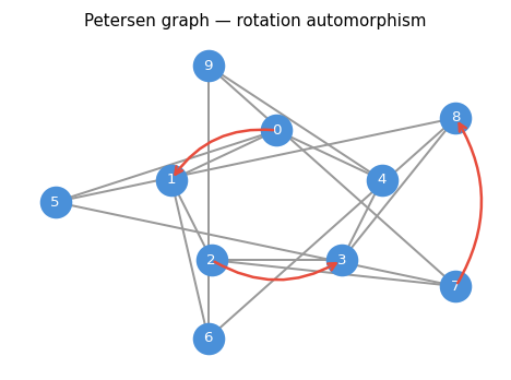
The Petersen graph, with arrows indicating one automorphism: a cyclic rotation of the outer ring.

The next two lemmas make precise the intuition that automorphisms are “invisible” symmetries — they cannot be detected by local measurements like degree or distance.

The proof works by transferring the local neighbourhood structure through the isomorphism; the same argument applies to any graph invariant that is determined locally around a vertex.

The proof proceeds by a clean bijection between paths: \(g\) maps every \(uv\)-walk of length \(\ell\) to a \(u^g v^g\)-walk of the same length, and \(g^{-1}\) reverses this bijection.

These two lemmas encode a powerful constraint: automorphisms act as symmetries that are invisible to local graph invariants like degree and distance. Any graph property invariant under relabelling is automatically preserved by automorphisms.

1.3 Homomorphisms

A homomorphism relaxes the isomorphism condition from a two-way implication to a one-way implication: edges must map to edges, but non-edges may also map to edges. This makes homomorphisms a vastly richer class of maps.

Homomorphisms arise naturally in graph colouring: assigning colours to vertices so that no two adjacent vertices share a colour is precisely a homomorphism into a complete graph. By relaxing the bijectivity and edge-reflection requirements of isomorphism, we obtain a framework that connects graph structure to chromatic properties.

The notation \(X \to Y\) defines a preorder on graphs: \(X \to X\) (via the identity), and if \(X \to Y\) and \(Y \to Z\) then \(X \to Z\) (by composition). This preorder organizes the entire universe of graphs according to their “homomorphic complexity.”

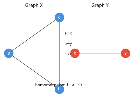
Left: triangle \(K_3\). Right: single edge \(K_2\). The map \(a \mapsto x, b \mapsto y, c \mapsto x\) is a valid homomorphism, sending a triangle to an edge — a non-injective map.

Homomorphisms are not required to be injective or surjective, and they need not reflect the edge relation. This flexibility makes them the right notion for graph colouring theory.

The following lemma makes the connection to colouring precise and is one of the most useful restatements of a classical concept in all of combinatorics.

This lemma is fundamental: graph colourings are exactly graph homomorphisms into complete graphs. The minimum such target is the chromatic number. Among homomorphisms, one particularly structured type plays a starring role in the theory of retracts and in algorithmic graph theory.

Intuitively, a retract is a subgraph that is “topologically inert” — the whole graph can be continuously collapsed onto it without tearing any edges. Retracts arise naturally in the study of core graphs and in the categorical theory of graph homomorphisms.

Chapter 2: Families of Graphs

This chapter surveys the three principal families of graphs that appear throughout algebraic graph theory: circulant graphs, Johnson graphs, and line graphs. Each arises naturally from algebraic or combinatorial constructions and possesses rich symmetry structure.

2.1 Circulant Graphs

The cycle \(C_n\) is the simplest example of a vertex-transitive graph, with automorphism group equal to the dihedral group \(D_{2n}\). Circulant graphs generalise cycles by allowing additional edge connections dictated by an arithmetic structure on \(\mathbb{Z}_n\).

To build a graph with a built-in cyclic symmetry, we need only decide which “steps” along \(\mathbb{Z}_n\) constitute edges — the arithmetic structure of the group does the rest.

The inverse-closure condition is precisely what makes the edge relation symmetric: if \(i\) is connected to \(j\) because \(i - j \in C\), then \(j - i = -(i-j) \in C\), so \(j\) is connected back to \(i\). The set \(C\) is called the connection set of the circulant.

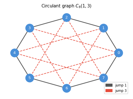
The circulant graph \(C_8(1,3)\): an 8-cycle (solid edges) augmented with “chord” connections of jump 3 (dashed red edges). The symmetry group acts by cyclic shifts and the reflection \(i \mapsto -i\).

The cyclic shift \(g : i \mapsto i+1\) and the reflection \(h : i \mapsto -i\) both belong to \(\mathrm{Aut}(X(\mathbb{Z}_n, C))\). The rotation subgroup \(R = \langle g \rangle\) and the coset \(hR\) are distinct, giving \(|\mathrm{Aut}(X(\mathbb{Z}_n, C))| \geq 2n\).

2.2 Johnson Graphs

Johnson graphs arise from set intersections and constitute a fundamental family in algebraic combinatorics.

If circulant graphs encode group arithmetic, Johnson graphs encode combinatorial arithmetic: here, the “vertices” are subsets of a ground set, and adjacency measures how much two subsets overlap. This shift from groups to sets yields a rich family that includes the Kneser graphs and the Petersen graph as key special cases.

The three parameters \((v, k, i)\) control the density and structure of the graph: increasing \(i\) requires more overlap for adjacency, making the graph sparser; decreasing \(i\) allows less overlap, making it denser. The entire Johnson scheme — the collection of all \(J(v,k,i)\) for fixed \(v,k\) — forms the basis of association scheme theory.

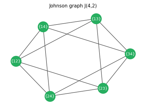
The Johnson graph \(J(4,2)\): vertices are 2-element subsets of \(\{1,2,3,4\}\), and two vertices are adjacent when their intersection has exactly 1 element. This is the octahedron graph.

Since every \(k\)-subset of \([v]\) plays the same role, we expect the graph to be regular — and it is.

The proof uses a clean double-counting argument: first fix the intersection, then count the ways to complete the neighbour. This regularity confirms that the graph looks the same from every vertex — an early hint of the vertex-transitivity we will prove shortly.

The isomorphism is given by complementation: \(S \mapsto \bar{S} = [v] \setminus S\). An important special case: the Kneser graphs \(J(v,k,0)\). In particular, \(J(5,2,0)\) is the Petersen graph, one of the most important graphs in combinatorics.

The automorphism group of the Johnson graph is at least as large as the symmetric group on \([v]\), since any permutation of the ground set induces a graph automorphism.

The key observation is that permutations of the ground set preserve intersection sizes — a clean example of a symmetry acting at one level (the ground set) inducing a symmetry at another level (the subsets). Typically \(\mathrm{Aut}(J(v,k,i)) \cong \mathrm{Sym}(v)\), but there are exceptions.

2.3 Line Graphs

The line graph construction replaces edges by vertices and adjacency by shared endpoints.

The line graph construction shifts perspective from vertices to edges: instead of asking how vertices relate to each other, we ask how edges interact. This “dual” viewpoint often simplifies spectral analysis and appears naturally in network flow and matching theory.

The definition encodes a simple geometric idea: two edges in a graph “interact” if they share a vertex — just as two roads intersect at a junction. The line graph makes this interaction structure into a new graph, amenable to the same algebraic techniques as any other graph.

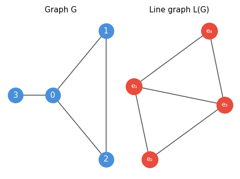
Left: a triangle with a pendant edge. Right: the corresponding line graph. Each edge of \(G\) becomes a vertex in \(L(G)\), with adjacencies reflecting shared endpoints.

If \(X \cong Y\) then \(L(X) \cong L(Y)\), but the converse fails: \(L(C_3) \cong L(K_{1,3})\) yet \(C_3 \not\cong K_{1,3}\). The converse does hold when both graphs have minimum degree at least 4. Not every graph is a line graph: for instance, \(K_{1,3}\) is not, since any preimage would need an edge incident to three others at a common endpoint, leading to a contradiction.

Line graphs appear prominently in spectral theory: if \(B = B(X)\) is the incidence matrix, then \(B^T B = 2I + A(L(X))\), and the positive semidefiniteness of \(B^T B\) immediately implies \(\lambda_{\min}(L(X)) \geq -2\).

Chapter 3: Group Actions on Graphs

Group actions provide the algebraic framework to study graph symmetry systematically. Instead of studying automorphisms of a specific graph in isolation, we study the action of abstract groups on sets and graphs.

3.1 Group Actions

To study graph symmetry systematically, we need the language of group actions. An abstract group acting on a set captures the idea of “symmetry” in a way that is both flexible and algebraically tractable.

With this in place, a group action is simply a homomorphism into a symmetric group.

A group action is faithful when no non-identity element acts trivially — every element of the group “does something” to the set. Faithfulness is the natural condition when we want to identify the group with a genuine set of symmetries, rather than a group that partially acts on the set.

We write \(v^g\) for \(f(g)(v)\), the image of \(v \in V\) under \(g \in G\). For \(S \subseteq V\), \(S^g = \{v^g : v \in S\}\). A subset \(S\) is \(G\)-invariant if \(S^g = S\) for all \(g \in G\).

Two fundamental concepts attach to every element of \(V\) under a group action: the orbit (all elements reachable from it) and the stabilizer (all group elements that fix it).

Orbits and stabilizers are complementary: the orbit measures how far the group can move \(x\), while the stabilizer measures how much of the group leaves \(x\) fixed. Together they partition the group action into structured pieces.

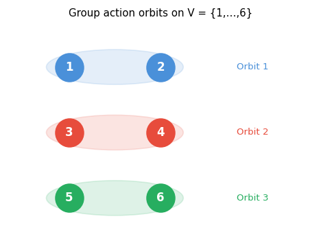
Three orbits of a group action on \(V = \{1,2,3,4,5,6\}\). The group permutes elements within each coloured oval but never moves elements between ovals.

The orbits partition \(V\) into disjoint \(G\)-invariant subsets. The stabilizer \(G_x\) is always a subgroup of \(G\).

3.2 The Orbit-Stabilizer Theorem

The Orbit-Stabilizer theorem is the cornerstone of enumeration in group theory. It relates the size of a group to the size of its orbits and stabilizers. The key preliminary observation is that the set of group elements sending \(x\) to any fixed \(y\) is not arbitrary — it forms an entire coset of the stabilizer.

This lemma reveals a clean partition of \(G\): each element of the orbit \(x^G\) corresponds to a unique coset of \(G_x\), giving the orbit-stabilizer theorem.

The proof constructs a bijection between orbit elements and cosets, then invokes Lagrange’s theorem. This is both elegant and powerful: it implies that the size of every orbit divides \(|G|\), a constraint that severely limits which subsets of \(V\) can be orbits.

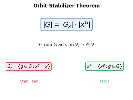
The Orbit-Stabilizer equation \(|G| = |G_x| \cdot |x^G|\): the group splits into cosets of the stabilizer, each coset corresponding to exactly one element of the orbit.

A key consequence involves the notion of conjugation.

The stabilizers along an orbit are all conjugate to each other, as the following lemma makes precise.

3.3 Burnside’s Lemma

Having established that orbits partition \(V\), the natural enumeration problem is: how many orbits are there? Burnside’s lemma gives a beautiful answer by converting the orbit-count into an average fixed-point count.

The proof is an elegant double-counting of the incidence set \(\Lambda\): the same set counted two ways yields, after dividing by \(|G|\), the number of orbits. This technique — picking a convenient auxiliary set and counting it in two ways — is one of the most versatile tools in combinatorics.

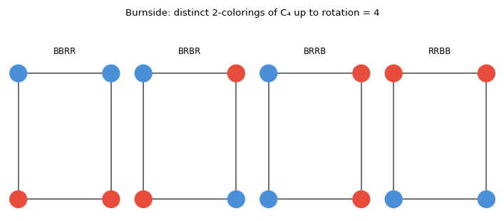
Four rotationally distinct 2-colourings of \(C_4\). Burnside’s lemma computes: \((16+0+4+0+4+0+16+0+\ldots)/8 = 6\) for necklaces, or \(4\) if only rotations are allowed.

Application to counting graph isomorphism classes. Let \(G = \mathrm{Sym}(n)\) act on \(\mathcal{G}_n\) (all graphs on \([n]\)) by \(X \mapsto X^g\). The orbits are exactly the isomorphism classes. Write \(\mathrm{Iso}(X) = \{Y \in \mathcal{G}_n : Y \cong X\}\) for the isomorphism class of \(X\).

Burnside then gives:

The key insight is that the identity permutation dominates the Burnside sum, contributing \(2^{\binom{n}{2}}\), while all other permutations contribute a negligible \(o(1)\) fraction.

3.4 Asymmetric Graphs

Burnside’s lemma gives us the tools to ask a fundamental probabilistic question: how symmetric is a “typical” graph? The answer is perhaps surprising.

Asymmetric graphs are those with no symmetry whatsoever — the only automorphism is the identity. The following theorem, while counterintuitive (highly structured objects seem interesting, yet typical objects have no structure), is one of the foundational results in random graph theory.

The proof exploits the asymmetry of counting: an asymmetric isomorphism class is exactly \(n!\) times larger than its representative, while a symmetric class is smaller by at least a factor of 2. This size advantage forces asymmetric classes to dominate.

3.5 Primitivity

When a group acts transitively on a set, it may or may not respect additional structure. This leads to the notion of primitive versus imprimitive actions, which is the analogue for group actions of the distinction between a prime and a composite number.

A block of imprimitivity is a subset that the group can only either entirely preserve or entirely move away from — a kind of indivisible “chunk” with respect to the action. The trivial blocks are singletons \(\{v\}\) and all of \(V\).

Primitivity is to group actions what primality is to integers: it identifies actions with no intermediate structure.

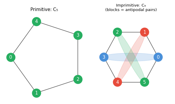
Left: \(C_5\) is primitive (prime \(n\), no non-trivial block structure). Right: \(C_6\) is imprimitive — the three coloured pairs of antipodal vertices form the blocks of imprimitivity.

The characterization of primitivity in terms of maximal subgroups is one of the deepest results of this chapter, connecting the geometric notion of a block structure to the algebraic notion of a maximal subgroup.

Both directions of the proof construct a bijection between the two types of intermediate structure — blocks on one side, intermediate subgroups on the other. This is a recurring pattern in group theory: geometric structure and algebraic structure shadow each other precisely.

Chapter 4: Transitive and Primitive Graphs

Transitivity conditions on graphs — vertex-transitivity, edge-transitivity, arc-transitivity — measure how “symmetric” a graph is. These properties have deep implications for graph structure, connectivity, and matchings.

4.1 Vertex-Transitive Graphs

With the group-theoretic machinery from Chapter 3 in place, we can now define and study transitivity conditions on graphs. These conditions measure how “symmetric” a graph is in a precise algebraic sense.

Intuitively, a vertex-transitive graph “looks the same from every vertex.” All such graphs are regular, since automorphisms preserve degree and can move any vertex to any other.

The \(k\)-cube is also a Cayley graph: \(Q_k = X(\mathbb{Z}_2^k, \{e_i : i \in [k]\})\), where \(e_i\) is the \(i\)-th standard basis vector. By the same left-multiplication argument, circulant graphs \(X(\mathbb{Z}_n, C)\) are vertex-transitive.

In general, \(J(v,k,i)\) are not Cayley graphs.

4.2 Cayley Graphs

Cayley graphs are the canonical examples of vertex-transitive graphs. They arise directly from the multiplication structure of a group — making explicit the connection between group theory and graph symmetry.

The idea is simple: take a group \(G\) and a generating set \(C\), and declare two group elements adjacent whenever one can be obtained from the other by multiplying by an element of \(C\). The resulting graph automatically inherits the group’s symmetry.

The condition \(1 \notin C\) ensures no loops; inverse-closure ensures undirectedness. The Cayley graph gives a visual and combinatorial representation of the group: its structure encodes how the generators interact and generate the whole group.

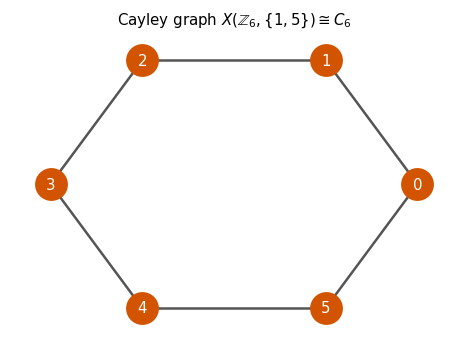
The Cayley graph \(X(\mathbb{Z}_6, \{1,5\}) \cong C_6\): the group \(\mathbb{Z}_6\) with generators \(\pm 1\) yields the 6-cycle. The left-multiplication maps \(\tau_g : x \mapsto gx\) act transitively on vertices.

The left-multiplication structure of the group immediately provides the required automorphisms.

This tells us that the group itself acts as a transitive subgroup of the automorphism group, via left multiplication. The transitive action of \(G\) on itself is called the regular representation, and it is the algebraic backbone of all Cayley graph constructions.

This clean equivalence means that connectivity of the Cayley graph reflects the generating property of \(C\): the graph is connected precisely when \(C\) is rich enough to “reach” the whole group from the identity by iterated multiplication.

Not every vertex-transitive graph is a Cayley graph. The Petersen graph \(J(5,2,0)\) is vertex-transitive but is not a Cayley graph, since neither \(\mathbb{Z}_{10}\) nor the dihedral group \(D_{10}\) produces a Cayley graph isomorphic to it.

To characterise exactly which vertex-transitive graphs are Cayley graphs, we use the notion of regularity for group actions.

This gives a clean characterisation: vertex-transitive graphs are precisely those admitting a regular subgroup in their automorphism group — which is exactly a Cayley graph structure.

Two Cayley graphs on the same group are isomorphic when their connection sets are related by a group automorphism.

Note that \(X(G,C) \cong X(G,\theta(C))\) does not require \(\theta\) to be an automorphism — the converse is false in general.

Furthermore:

4.3 Edge-Transitive and Arc-Transitive Graphs

Beyond vertex-transitivity, we can ask whether the automorphism group acts transitively on edges or on directed edges (arcs). These finer conditions capture increasingly strong symmetry requirements.

Arc-transitivity is strictly stronger than edge-transitivity: an arc-transitive automorphism can not only carry any edge to any other, but can also reverse the direction of any edge. Equivalently, for any two arcs \((u,v)\) and \((x,y)\), there is an automorphism sending \(u \mapsto x\) and \(v \mapsto y\). Arc-transitivity implies both vertex and edge transitivity, but the converses fail. The triangular prism is vertex-transitive but not edge-transitive; \(K_{n,m}\) for \(n \neq m\) is edge-transitive but not vertex-transitive.

The proof uses the concept of an oriented graph.

The proof exploits the parity of the two arc-orbits: if they are distinct, the indegree equals the outdegree in the oriented graph \(\Omega_1\), forcing the total degree to be even.

4.4 Connectivity and Matchings of Vertex-Transitive Graphs

The symmetry of vertex-transitive graphs constrains their connectivity and matching properties in remarkable ways. These results show that high symmetry forces high connectivity — a striking instance of algebraic structure controlling combinatorial properties.

For general graphs, the edge connectivity can be as small as the minimum degree. For vertex-transitive graphs, vertex symmetry forces a much tighter result. Two preparatory lemmas are needed.

The proof is a beautiful interplay between graph theory and group theory: edge atoms are used to construct blocks of imprimitivity, and the block structure then gives the lower bound on connectivity by a direct counting argument.

This bound is tight for certain families of graphs.

The matching theory of vertex-transitive graphs rests on two structural lemmas. A vertex is critical if it is saturated in every maximum matching.

This is proved by a careful induction on vertices and edges, using the vertex-transitivity to propagate matching properties from subgraphs back to \(X\).

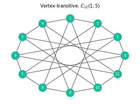
The circulant \(C_{12}(1,5)\): a vertex-transitive graph on 12 vertices. Every vertex has degree 4, and the automorphism group acts transitively — every vertex looks identical.

Chapter 5: Eigenvalues and the Adjacency Matrix

The second major algebraic tool in graph theory is linear algebra: the adjacency matrix and the spectrum of its eigenvalues encode surprising information about graph structure.

5.1 The Adjacency Matrix and Spectrum

The adjacency matrix is the bridge between combinatorics and linear algebra. Once we encode a graph as a matrix, the full machinery of linear algebra — eigenvalues, eigenvectors, spectral decompositions — becomes available.

The symmetry of \(A\) is not incidental — it is the matrix-theoretic reflection of the graph’s undirectedness, and it guarantees that all eigenvalues are real and that the matrix is orthogonally diagonalizable. This makes spectral graph theory possible.

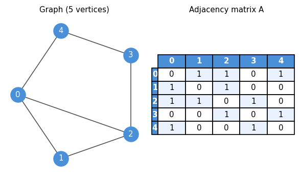
A 5-vertex graph alongside its adjacency matrix. The symmetry \(A = A^T\) reflects the undirectedness of the graph; the zero diagonal reflects the absence of loops.

Since \(A(X)\) is real and symmetric, all its eigenvalues are real and it has an orthonormal eigenvector basis. Isomorphic graphs have the same spectrum — but the converse fails (non-isomorphic graphs can be cospectral). The existence of cospectral non-isomorphic graphs is a fundamental limitation of the spectral approach: eigenvalues do not fully classify graphs, and the study of graph invariants that go beyond the spectrum is an active research area.

Computing eigenvalues. If \(f : V(X) \to \mathbb{R}\) satisfies \(\sum_{v \sim u} f(v) = \lambda f(u)\) for all \(u\), then \(\lambda\) is an eigenvalue of \(A(X)\) with eigenvector \(f\).

5.2 Incidence Matrix and the Laplacian

The adjacency matrix is not the only natural matrix associated to a graph. The incidence matrix encodes how vertices relate to edges, and it leads to the Laplacian — perhaps the most analytically rich matrix in all of spectral graph theory.

The incidence matrix records vertex-edge membership rather than vertex-vertex adjacency. Its rank captures how many “independent” ways to traverse the graph — a fact made precise by the following theorem.

The proof characterizes the null space of \(B^T\) directly: the only “harmonic” signed vertex-labellings are those that alternate \(\pm 1\) on bipartition classes, one degree of freedom per bipartite component.

The key matrix identity \(BB^T = D(X) + A(X)\) (where \(D\) is the diagonal degree matrix) and \(B^T B = 2I + A(L(X))\) connect the incidence matrix to both the adjacency matrix and the line graph.

The Laplacian might initially look like a slight variation on the adjacency matrix, but it is far more — it encodes the graph’s connectivity, flow, and expansion properties in a single matrix, and its eigenvalues govern everything from random walks to network robustness.

The Laplacian measures the “roughness” of a function on the graph: \(x^T L x\) is large when adjacent vertices have very different \(x\)-values. The smallest eigenvalue of \(L\) is always 0 (with eigenvector \(\mathbf{1}\)), and:

5.3 Symmetric Matrices and the Spectral Theorem

Since \(A(X)\) is real symmetric, the spectral theorem applies in full. The key properties are:

• Eigenvectors for distinct eigenvalues are orthogonal.
• All eigenvalues are real.
• \(\mathbb{R}^n\) has an orthonormal eigenvector basis.
• \(A = P D P^T\) for orthogonal \(P\), giving \(A = \sum_{i=1}^n \lambda_i v_i v_i^T\).

5.4 The Courant-Fisher Theorem

The Courant-Fisher theorem characterises eigenvalues as solutions to min-max optimisation problems over the Rayleigh quotient — a perspective that connects spectral theory to variational calculus and turns eigenvalue bounds into optimization problems.

The Rayleigh quotient measures, for a given direction \(x\), how much the matrix \(A\) “stretches” in that direction. Maximizing it gives the largest eigenvalue; more generally, a min-max characterization gives every eigenvalue.

The proof uses a dimension-counting argument: any \(k\)-dimensional subspace must intersect the bottom \((n-k+1)\)-dimensional eigenspace nontrivially, providing a vector with Rayleigh quotient at most \(\lambda_k\). This intersection argument is the core of many spectral bounds in combinatorics.

5.5 The Maximum Eigenvalue

Among all eigenvalues, the largest — called the spectral radius — has the most direct combinatorial interpretation: it measures how well-connected the graph is on average, and bounds the chromatic number from above.

The lower bound uses the constant vector as a test vector in the Rayleigh quotient; the upper bound localizes at the vertex of maximum eigenvector weight. Together, they sandwich \(\lambda_1\) between two natural degree-based quantities.

This is a spectacular result: a purely spectral quantity (the largest eigenvalue) controls the chromatic number — a property that in general requires exponential computation to determine. The proof is an inductive vertex-deletion argument, with interlacing providing the key hereditary property.

5.6 Eigenvalue Interlacing

Interlacing theorems are the spectral analogue of the inclusion-exclusion principle: when a graph is reduced by deleting a vertex or restricting to an induced subgraph, the eigenvalues of the smaller graph are interleaved with those of the larger graph. This is one of the most powerful techniques in spectral graph theory.

Interlacing shows that removing a vertex from a graph cannot decrease the minimum eigenvalue or increase the maximum eigenvalue. In other words, the extreme eigenvalues are “monotone” under induced subgraph taking — a fact used constantly in spectral arguments. Combined with the positive semidefinite matrix argument, this gives:

5.7 Perron-Frobenius Theorem

The Perron-Frobenius theorem is the spectral theorem of nonnegative matrix theory, and for connected graphs it reveals a striking rigidity: the largest eigenvalue is simple, achieved by a strictly positive eigenvector, and its magnitude controls the symmetry of the spectrum.

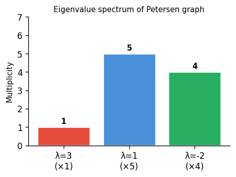
Eigenvalue spectrum of the Petersen graph: eigenvalue 3 (multiplicity 1), eigenvalue 1 (multiplicity 5), eigenvalue \(-2\) (multiplicity 4). The Petersen graph is 3-regular, and \(\lambda_1 = 3\) confirms regularity.

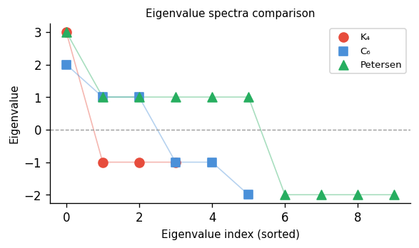
Comparing spectra of \(K_4\), \(C_6\), and the Petersen graph. \(K_4\) has one large eigenvalue; \(C_6\)’s spectrum is symmetric (bipartite complement); the Petersen graph has a characteristic gap between \(\lambda_1=3\) and \(\lambda_2=1\).

5.8 Strongly Regular Graphs

The spectrum of a graph encodes a great deal of information, but for a very special class of graphs — the strongly regular graphs — the spectrum is essentially determined by the combinatorial parameters and vice versa. This makes strongly regular graphs both highly structured and highly constrained.

Why are strongly regular graphs (SRGs) so interesting? They occupy a remarkable middle ground in the landscape of graphs. A random graph looks different from every vertex and every pair of vertices; a complete graph looks the same but is trivially uniform. Strongly regular graphs are neither: they are highly non-trivial, yet they impose an iron uniformity on every pair of vertices simultaneously. This tension between structure and non-triviality makes them the central objects of algebraic combinatorics.

They arise naturally in many areas of mathematics. In finite geometry, the points of a projective or polar space form an SRG. In coding theory, the minimum-weight codewords of a linear code often form the vertices of an SRG, with the graph encoding the combinatorial structure of the code. In design theory, every symmetric 2-design gives rise to an SRG on its points. In group theory, the orbital graphs of rank-3 permutation groups are always strongly regular — this is one of the central reasons that the classification of rank-3 groups (a chapter in the classification of finite simple groups) is intimately tied to the theory of SRGs. And in spectral graph theory, SRGs provide the cleanest examples of the three-eigenvalue phenomenon we are about to prove.

The parameters \((n, k, a, c)\) are simple to state but severely constraining. Most tuples \((n, k, a, c)\) satisfying even obvious necessary conditions — the parameter equation, the integrality of eigenvalue multiplicities — turn out not to be realizable by any actual graph. Determining whether a given parameter set is realizable, and if so, how many non-isomorphic SRGs have those parameters, is one of the central open problems in algebraic combinatorics. Some parameter sets admit a unique graph (up to isomorphism); others admit thousands; some admit none at all. This unpredictability is part of what makes the subject so rich and difficult.

The definition imposes a remarkable uniformity: not only is the graph regular (every vertex has the same degree), but every pair of vertices has the same number of common neighbours — a property depending only on whether they are adjacent. This is a dramatically stronger condition than regularity alone.

The complement of a strongly regular graph is also strongly regular.

A strongly regular graph is primitive if both it and its complement are connected.

The complement of a strongly regular graph is also strongly regular, which immediately doubles our supply of examples and tells us that SRGs come in complementary pairs.

The four parameters \((n,k,a,c)\) are not independent — they satisfy a necessary integrality and consistency condition. Think of this as a bookkeeping identity: fixing a vertex \(u\) and counting the edges between its neighbourhood \(N(u)\) and its non-neighbourhood \(\bar{N}(u) = V \setminus (N(u) \cup \{u\})\) in two ways must give the same answer. This kind of double-counting argument is one of the foundational techniques of combinatorics, and here it immediately yields a strong constraint.

The proof is a clean double-counting of a bipartite graph between the neighbourhood and non-neighbourhood of a fixed vertex. This relation is a useful first check: any putative parameter set \((n,k,a,c)\) failing this identity cannot be realized by a strongly regular graph.

Now we arrive at the spectral core of the theory. The key algebraic identity for SRGs is that \(A^2 = kI + aA + c(J-I-A)\), which comes directly from the definition: the \((u,v)\)-entry of \(A^2\) counts walks of length 2 from \(u\) to \(v\), and for an SRG this count depends only on whether \(u \sim v\) (giving \(a\)) or \(u \not\sim v\) (giving \(c\)). This matrix equation constrains the minimal polynomial of \(A\), and that constraint forces there to be at most three eigenvalues.

Conversely, a connected regular graph with exactly three distinct eigenvalues is strongly regular — and this converse is also true. This is a beautiful rigidity result: the spectral data (number of distinct eigenvalues) forces the combinatorial data (exact common-neighbour counts). The three eigenvalues and the SRG parameters completely determine each other, making SRGs one of the most tightly controlled families in all of combinatorics.

The requirement that \(m_\theta, m_\tau\) be positive integers is a strong integrality constraint on the parameters \((n,k,a,c)\). It rules out vast families of parameter tuples that otherwise satisfy the parameter relation. When \(\Delta = (a-c)^2 + 4(k-c)\) is a perfect square, the multiplicities are automatically integers. When it is not, the multiplicities can still be integers but the constraint becomes more subtle — this is the case of “irrational” SRGs, which are particularly hard to construct or rule out, and where the interplay between number theory and combinatorics is most vivid.

5.9 Paley Graphs

The Paley graphs are a remarkable family that sits at the intersection of number theory, algebra, and combinatorics. They are constructed from finite fields and provide concrete examples of strongly regular, arc-transitive, self-complementary graphs — a rare combination of desirable properties.

The condition \(q \equiv 1 \pmod 4\) ensures \(-1\) is a square in \(\mathrm{GF}(q)\), which is precisely what makes the edge relation symmetric: \(u - v\) is a square if and only if \(v - u = -(u-v)\) is a square. Without this condition, the graph would be a tournament rather than an undirected graph.

The condition \(q \equiv 1 \pmod 4\) ensures that \(-1\) is a square in \(\mathrm{GF}(q)\), making the edge relation symmetric. Paley graphs are \(\frac{q-1}{2}\)-regular and arc-transitive.

Beyond Paley graphs, there are several other important families of strongly regular graphs.

The lattice graph \(L_n\) is the special case where the Latin square is the addition table of \(\mathbb{Z}_n\).

5.10 Expanders and the Second Eigenvalue

The second eigenvalue of the Laplacian, \(\mu_2\), measures how well-connected a graph is beyond mere connectivity. A graph with large \(\mu_2\) is a good expander: every small set of vertices has many edges leaving it.

Expanders are among the most important objects in theoretical computer science and combinatorics. The motivation is practical: in communication networks, you want a graph that is simultaneously sparse (cheap to build, few connections per node) and highly connected (messages can propagate quickly, with no “bottlenecks” where traffic is forced through a tiny cut). These two desiderata are in apparent tension — sparse graphs should have poor connectivity — but expanders achieve both simultaneously. The spectral gap \(\mu_2\) is the mathematical measure of expansion: a large gap means no small cut exists relative to the set’s size. The Cheeger inequality below makes this precise, relating a purely algebraic quantity (an eigenvalue) to a purely combinatorial one (the minimum boundary-to-volume ratio).

This inequality — sometimes called the Cheeger inequality for graphs — is one of the most important results in spectral graph theory. It says that a graph with a large spectral gap \(\mu_2\) is necessarily a good expander. The proof is a clean application of Courant-Fisher: choose a test vector that is the characteristic function of \(S\), shifted to be orthogonal to \(\mathbf{1}\), and evaluate the Rayleigh quotient for the Laplacian.

The converse direction — that expanders have large \(\mu_2\) — is also true (and slightly harder): \(\mu_2 \geq \theta(X)^2 / 2k\) for \(k\)-regular graphs. Together, the two directions say that \(\mu_2\) and \(\theta(X)\) are within a polynomial factor of each other, making the spectral gap and the combinatorial expansion equivalent up to polynomial losses.

The study of graph families with simultaneously large degree and large \(\mu_2\) is the theory of Ramanujan graphs. A \(k\)-regular Ramanujan graph achieves the optimal spectral gap: \(\lambda_2 \leq 2\sqrt{k-1}\). This bound, proved by the Alon-Boppana theorem, is optimal — no sequence of \(k\)-regular graphs can do better. Explicit constructions of Ramanujan graphs (by Lubotzky-Phillips-Sarnak and Margulis) use deep number theory (the Ramanujan conjecture, now a theorem of Deligne) and show that the worlds of spectral graph theory, finite group theory, and analytic number theory are intimately connected.

Chapter 6: Generalized Polygons

Incidence geometry provides a rich source of highly symmetric graphs. In this chapter we study incidence structures, projective planes, and their associated bipartite graphs (incidence graphs). The key insight is that projective planes correspond exactly to bipartite graphs of diameter 3 and girth 6.

Up to now, our graphs have come from groups (Cayley graphs, circulants), from set combinatorics (Johnson graphs), or from matrix spectra (strongly regular graphs). This chapter opens a completely different door: classical incidence geometry. The objects here — projective planes, generalized polygons — were studied by geometers long before graph theory existed, and yet they produce some of the most symmetric, most structurally rigid graphs known.

The central idea is to convert a geometric system (points and lines with an incidence relation) into a graph, called the incidence graph or Levi graph. This translation is lossless: every property of the geometry can be read off from the graph, and vice versa. The payoff is that powerful graph-theoretic and algebraic tools — automorphism groups, eigenvalue bounds, girth-diameter relations — all become available to study geometric structures.

Projective planes in particular sit at a remarkable intersection: they arise from finite fields (the construction \(PG(2,q)\) below), they are characterized by a beautifully clean diameter-girth condition on their incidence graphs, and their automorphism groups turn out to be linear groups over the field. Understanding this chapter means understanding why the geometry of finite fields and the combinatorics of graphs are two faces of the same mathematical object.

6.1 Incidence Structures and Incidence Graphs

The dual \(\mathcal{I}^* = (\mathcal{L}, P, I^*)\) where \(I^* = \{(L, p) : (p,L) \in I\}\) swaps the roles of points and lines. Many important incidence structures are self-dual. Duality is a deep organizing principle: a theorem about points and lines automatically yields a theorem about lines and points, at no extra cost.

To bring graph-theoretic tools to bear on incidence structures, we encode the geometry as a bipartite graph.

The incidence graph is the Rosetta Stone of this chapter: geometric properties of \(\mathcal{I}\) (how many points lie on a line, how many lines pass through a point, when two lines meet) translate directly into graph-theoretic properties (regularity, degree, girth, diameter). The bipartiteness is automatic: edges always run between the point-side and the line-side, never within either side. An automorphism of \(\mathcal{I}\) that preserves point-and line-types becomes exactly a graph automorphism that preserves the bipartition. Translating incidence geometry into graph theory allows us to apply spectral and automorphism-group techniques.

Notice that the automorphism group of \(\mathcal{I}\) embeds naturally into the automorphism group of its incidence graph \(X(\mathcal{I})\). This is one of the key tools we will exploit: by studying the incidence graph’s symmetry, we learn about the symmetry of the underlying geometry.

There is a subtle point here that is easy to miss: the automorphism group of \(X(\mathcal{I})\) may be strictly larger than the automorphism group of \(\mathcal{I}\). The incidence graph is a bipartite graph, and an automorphism of the graph might swap the two sides — swapping all points with all lines. This corresponds to a duality of the incidence structure, a concept that is meaningful only for self-dual geometries. For projective planes, which are self-dual, these “improper” automorphisms (dualities) are geometrically meaningful and important. For non-self-dual geometries, they are graph automorphisms that have no geometric interpretation. This distinction will matter when we analyze the automorphism group of \(PG(2,q)\).

6.2 Partial Linear Spaces

Before reaching the full definition of a projective plane, we introduce the key regularity axiom that geometries must satisfy. In a “nice” incidence structure, any two points should determine at most one line — just as in the Euclidean plane, two points determine a unique line. This is the defining property of a partial linear space.

This lemma says that the “at most one” condition is symmetric in points and lines — it holds for lines as well as points. This is the first hint that duality is a deep feature of the theory.

Two lines incident with a common point are called concurrent. The girth constraint on the incidence graph captures the partial linearity condition exactly. This is the graph-theoretic translation of the geometric axiom, and it is the key lemma that allows us to pass freely between the geometric and graph-theoretic perspectives.

The proof is a one-sentence geometric-to-combinatorial translation: a 4-cycle in the incidence graph says precisely that two points lie on two common lines, which is forbidden. This establishes a clean lower bound on the girth of incidence graphs of “reasonable” geometries — and projective planes will turn out to achieve the girth exactly as small as possible while also being as “connected” as possible.

This girth-6 lower bound is part of a general phenomenon in extremal graph theory: the girth of an incidence graph is tightly controlled by the “complexity” of the geometry. Affine planes (projective planes with one line removed) have incidence graphs of girth 6 and diameter 4; projective planes achieve diameter 3, which is optimal. This optimality — girth 6 and diameter 3 simultaneously — is precisely the Moore bound for bipartite graphs of girth 6, and it is one of the most striking manifestations of the connection between geometry and extremal combinatorics.

6.3 Projective Planes

We now arrive at the central geometric object of this chapter. A projective plane is what you get when you take the ordinary Euclidean plane and add “points at infinity” to ensure that every pair of lines meets — eliminating the special case of parallel lines. The result is a geometry so symmetric that it is, in a precise sense, the simplest non-trivial geometry.

Why should algebraic graph theorists care about projective planes? There are several reasons. First, their incidence graphs are among the most highly symmetric bipartite graphs known — they are arc-transitive, and their automorphism groups are classical linear groups. Second, these incidence graphs achieve an extremal property: for a given vertex degree (corresponding to the order of the plane), they simultaneously maximize girth and minimize diameter among all bipartite graphs — a combinatorial miracle called the Moore bound. Third, the eigenvalues of the incidence graph can be computed explicitly from the order of the plane, and these eigenvalues control expansion and mixing properties that have applications to coding theory and computer science.

Conditions (C1) and (C2) are exact duals of each other — swapping “points” and “lines” converts one into the other. This is the principle of projective duality: every theorem about a projective plane yields a dual theorem for free, by swapping points and lines throughout. Condition (C3) is a nondegeneracy condition that rules out trivial “planes” consisting of a single line with all points on it.

Let us pause to appreciate why axiom (C1) — any two distinct lines meet in a unique point — represents such a clean conceptual move from the Euclidean setting. In the ordinary Euclidean plane, two lines either meet in a unique point or are parallel. The existence of parallel lines is an anomaly — a special case that forces geometric arguments to split into cases. Projective geometry eliminates this anomaly by postulating that “points at infinity” exist, one for each direction, and that parallel lines meet at the corresponding point at infinity. The projective plane is the completion of the Euclidean plane under this extension, and it is dramatically more symmetric: there are no special lines, no special points, and every pair of lines meets exactly once.

The finite case captures the same spirit: in \(PG(2,q)\), every two lines meet in exactly one point. The classical Euclidean messiness of parallelism simply disappears. What remains is a perfectly symmetric geometry on \(q^2+q+1\) points, where every line contains exactly \(q+1\) points and every point lies on exactly \(q+1\) lines. This symmetry is so complete that the geometry looks identical from the perspective of any incident point-line pair — the defining property of arc-transitivity, which we will prove in Section 6.4.

A useful consequence: if a projective plane has any line with \(n+1\) points on it, then every line has exactly \(n+1\) points and every point lies on exactly \(n+1\) lines. The integer \(n\) is called the order of the projective plane, and the total number of points (and lines) is \(n^2 + n + 1\). For \(n=2\), this gives the Fano plane — 7 points and 7 lines, every line containing 3 points, every point on 3 lines. It is the smallest projective plane and one of the most important combinatorial objects in mathematics.

The following theorem gives a clean graph-theoretic characterisation of projective planes, connecting combinatorial geometry to spectral graph theory. It is the payoff of the entire incidence-graph translation program: geometric axioms on points and lines become conditions on diameter and girth.

This theorem is remarkable: it says that the axioms of projective geometry — expressed in terms of points, lines, and incidence — are equivalent to two simple numerical conditions on a bipartite graph. The girth condition (at least 6) encodes the partial linearity; the diameter condition (exactly 3) encodes that any two elements are “connected” in the strongest possible sense. Graphs achieving both simultaneously are called cages in this context, and projective planes give the unique family of regular bipartite cages of diameter 3 — the so-called (q+1,6)-cages. This connects incidence geometry to the famous cage problem in extremal graph theory.

The theorem also reveals why the incidence graph is the right object to study, rather than some other graph derived from the geometry. The two key axioms of a projective plane — (C1) uniqueness of line through two points, (C2) uniqueness of intersection point of two lines — become the two key numerical conditions on the graph. The translation is lossless, and working with the graph gives us access to the entire toolkit of algebraic graph theory: degree sequences, girth bounds, spectral methods, automorphism groups. All of these will be deployed in what follows.

A word on what is not yet known: projective planes need not arise from finite fields. There exist projective planes of order \(n\) for all prime powers \(n\), but it is an open problem whether any projective plane of non-prime-power order exists. The order-10 case was settled by an exhaustive computer search (Lam, 1991) — no projective plane of order 10 exists. For other non-prime-power orders, the question remains wide open. This is one of the most tantalizing open problems in finite combinatorics, and it illustrates how constrained these geometric structures really are.

6.4 A Family of Projective Planes: \(PG(2,q)\)

We have seen that projective planes exist (at least in the abstract sense of the axioms), but do concrete, explicit families exist? The answer is yes, and the construction uses finite fields in a beautiful way.

Fix a prime power \(q\) and the finite field \(\mathbb{F}_q\). Let \(V = \mathbb{F}_q^3\). The projective plane \(PG(2,q)\) is the incidence structure where \(P\) consists of all 1-dimensional subspaces of \(V\), \(\mathcal{L}\) consists of all 2-dimensional subspaces, and incidence is subspace containment.

The notation “\(PG\)” stands for “projective geometry.” The construction is the finite analogue of the real projective plane \(\mathbb{RP}^2\): instead of lines through the origin in \(\mathbb{R}^3\), we take lines through the origin in \(\mathbb{F}_q^3\). The finite field replaces the real numbers, and the result is a finite combinatorial object with all the essential properties of a projective plane.

Since \(|\mathbb{F}_q^3 \setminus \{0\}| = q^3 - 1\) and each 1-dimensional subspace contains \(q-1\) nonzero vectors, we get \(|P| = |{\mathcal{L}}| = 1 + q + q^2\). Each line contains \(1 + q\) points and each point lies on \(1 + q\) lines, so \(X(PG(2,q))\) has \(2(q^2+q+1)\) vertices and is \((q+1)\)-regular. The case \(q = 2\) gives the Fano plane.

The counting here is a clean exercise in linear algebra over finite fields: the number of nonzero vectors in \(\mathbb{F}_q^3\) is \(q^3-1\), and dividing by \(q-1\) (the size of each nonzero scalar multiple class) gives the number of 1-dimensional subspaces. The same argument for 2-dimensional subspaces — via their annihilators in the dual space — shows that \(|P| = |\mathcal{L}|\), confirming the self-duality of \(PG(2,q)\).

This self-duality is not a coincidence: in \(PG(2,q)\), there is a canonical bijection between points and lines given by orthogonal complementation (using the standard inner product on \(\mathbb{F}_q^3\)). The point \(\mathrm{span}\{u\}\) is dual to the line \(\{v : u \cdot v = 0\} = u^\perp\). This duality is a fundamental symmetry of the construction and explains why so many results about \(PG(2,q)\) come in symmetric pairs.

Now let us verify that this construction actually satisfies the axioms of a projective plane. The proof is a direct exercise in linear algebra over \(\mathbb{F}_q\) — the three axioms translate into three standard linear-algebraic facts about subspaces of a 3-dimensional vector space over a finite field.

The automorphism group of \(PG(2,q)\) is extraordinarily rich, and understanding it is one of the central goals of the classical theory of projective geometry. The general linear group \(GL(3,q)\) acts on \(V\) and induces automorphisms of the projective plane. But since scalar multiples of the identity act trivially on subspaces, the “effective” group of linear automorphisms is the projective linear group \(PGL(3,q) = GL(3,q)/Z\), where \(Z\) is the scalar subgroup. In addition, field automorphisms of \(\mathbb{F}_q\) also induce automorphisms of \(PG(2,q)\), giving the full automorphism group \(P\Gamma L(3,q)\). This group is a finite simple group (up to small modifications), and its structure is one of the crown jewels of the classification of finite simple groups.

The key observation is that \(GL(3,q)\) preserves subspace containment: if \(U \subseteq W\) then \(A(U) \subseteq A(W)\) for any invertible linear map \(A\). Since incidence in \(PG(2,q)\) is defined by subspace containment, invertible linear maps automatically preserve incidence. The next two lemmas make this precise.

The fact that \(GL(3,q)\) acts as automorphisms is powerful, but the group is large and redundant: scalar matrices \(\lambda I\) act trivially on every subspace (since \(\mathrm{span}\{\lambda u\} = \mathrm{span}\{u\}\)). The “effective” group is thus \(PGL(3,q)\), which has order \(q^3(q^3-1)(q^2-1)/(q-1)\). For \(q = 2\) (the Fano plane), this gives \(|\mathrm{Aut}(PG(2,2))| = 168\), which is the well-known simple group \(PSL(2,7)\), the smallest non-abelian simple group after \(A_5\).

The incidence graph of \(PG(2,q)\) has the strongest possible symmetry. This is the culmination of the chapter: we started with a geometric object defined by simple linear-algebra axioms, translated it into a bipartite graph, and now discover that this graph is arc-transitive — the automorphism group acts transitively on directed edges, meaning the graph “looks the same” from every incident point-line pair.

To establish arc-transitivity, we need to show two things: (1) for any two incident pairs \((p_1, L_1)\) and \((p_2, L_2)\), there is an automorphism mapping one to the other; and (2) for any incident pair \((p, L)\), there is an automorphism mapping the arc \((p, L)\) to \((L, p)\) — i.e., reversing the direction. The first follows from the transitivity of \(GL(3,q)\) on ordered bases; the second follows from the self-duality of \(PG(2,q)\).

The proof illustrates the power of the linear-algebraic construction: arc-transitivity reduces to the ability of \(GL(3,q)\) to map any ordered basis to any other — which is precisely the defining property of invertible linear maps. The geometry does the heavy lifting for us.

Arc-transitivity means the incidence graph of \(PG(2,q)\) is, in a strong sense, the most uniform possible bipartite graph at its parameters. Combined with the girth-diameter characterization of Theorem 4.2.1, this makes \(X(PG(2,q))\) an extremal object in multiple senses simultaneously: extremal in girth, extremal in diameter, extremal in symmetry. These extremal properties make it a central example in algebraic graph theory and a testing ground for conjectures about symmetric graphs.

To summarize what we have built: starting from the finite field \(\mathbb{F}_q\), we construct the vector space \(\mathbb{F}_q^3\) and form the projective plane \(PG(2,q)\) by taking 1-dimensional and 2-dimensional subspaces as points and lines. The incidence graph \(X(PG(2,q))\) is a \((q+1)\)-regular bipartite graph on \(2(q^2+q+1)\) vertices with girth 6 and diameter 3. It is arc-transitive with automorphism group containing \(PGL(3,q)\). It achieves the Moore bound for bipartite graphs of degree \(q+1\) and girth 6. It is the most symmetric, most extremal graph we have encountered in this course, and it connects finite geometry, linear algebra over finite fields, and the theory of symmetric graphs in a single beautiful object.

Chapter 7: Homomorphisms, Cores, and Products

The theory of graph homomorphisms develops a rich categorical structure on the class of all graphs. Two central notions emerge: the core of a graph (its minimal homomorphic image) and the direct product (which represents homomorphisms universally). Together they give a lattice structure on the set of graph isomorphism classes.

We encountered homomorphisms in Chapter 1, where the key example was graph coloring: a proper \(k\)-coloring of \(X\) is precisely a homomorphism \(X \to K_k\). At the time, homomorphisms were a convenient language for coloring. In this chapter, we develop them as a subject in their own right, revealing a rich algebraic structure on the entire class of graphs.

The central question is: what does the homomorphism preorder \(X \to Y\) look like? Which graphs can be mapped to which? The answer involves two key ideas. First, the core of a graph: every graph \(X\) can be “compressed” to a unique minimal subgraph \(X^\bullet\) that captures all the homomorphic information of \(X\). Two graphs are homomorphically equivalent precisely when they have isomorphic cores. This makes cores the “canonical representatives” of equivalence classes — think of them as the simplest graph in each equivalence class, the one with no redundant structure.

Second, the direct product \(X \times Y\): this construction satisfies a universal property exactly analogous to the categorical product, making the class of graphs (modulo homomorphic equivalence) into a lattice. This connects graph theory to category theory in a precise way: graphs form a category, homomorphisms are morphisms, and products and coproducts exist with the expected universal properties.

The upshot is that graph homomorphisms are not merely a convenience for coloring theory — they organize all graphs into a structured hierarchy, with cores as the minimal elements of each class and the direct product giving the operation that “combines” two graphs in the most efficient way.

7.1 Basic Results on Homomorphisms

We begin by establishing the basic algebraic properties of the homomorphism relation. These are simple to state and verify, but they determine the overall structure of the theory.

Before diving into the lemmas, let us ground ourselves in the category-theoretic perspective. Graphs form a category \(\mathbf{Graph}\): objects are graphs, morphisms are homomorphisms, the identity morphism is the identity map, and composition is function composition. In this language, the homomorphism relation \(X \to Y\) says precisely that there is a morphism from \(X\) to \(Y\). The preorder structure of \(\to\) is then the coarse structure of the category: which objects can be mapped to which.

Category theory tells us that this preorder structure is deeply connected to the existence of categorical products and coproducts — and indeed, we will see in Section 7.3 that the direct product of graphs is exactly the categorical product in \(\mathbf{Graph}\). The coproduct is the disjoint union. This is not a formal observation but a theorem with content: it gives the direct product a universal property, which will be our main tool for analyzing the lattice of cores.

This means \(\to\) is a preorder, not a partial order, on the class of all graphs. Reflexivity is the identity map; transitivity is composition of homomorphisms. The failure of antisymmetry is the interesting part: there exist non-isomorphic graphs \(X\) and \(Y\) with \(X \to Y\) and \(Y \to X\). This is precisely why we need the notion of homomorphic equivalence to get a partial order.

Homomorphic equivalence is the right notion of “sameness” for homomorphism theory, coarser than isomorphism. Two graphs are homomorphically equivalent when they can be mapped to each other — they are “the same” in the homomorphism preorder. For example, any graph is homomorphically equivalent to its core (since we can map the graph to the core and include the core back). In contrast, isomorphic graphs are of course homomorphically equivalent, but the converse is wildly false: a triangle \(K_3\) and any odd cycle \(C_{2k+1}\) are all homomorphically equivalent (they can all map to each other), but they are not isomorphic. This is what makes the core — the unique minimal representative of each equivalence class — such a valuable object.

Surjectivity is the key hypothesis here. Without it, \(X \to Y \to X\) could “fold” \(X\) down and then “expand” it back, arriving at a different graph. The lemma says that surjective homomorphisms in both directions are so constraining that they force isomorphism — a rigidity result that will be central in our analysis of cores.

One of the most powerful tools for showing that a homomorphism does not exist is to use invariants that are monotone with respect to \(\to\). Two such invariants are the chromatic number and the odd girth. The general strategy is: to prove \(X \not\to Y\), find a monotone invariant \(\phi\) and show \(\phi(X) > \phi(Y)\). The chromatic number and odd girth are the two most useful such invariants in practice, because they are computable and reflect genuinely different aspects of graph structure.

Lemma 5.1.3 is our main obstruction tool: to show \(X \not\to Y\), it suffices to exhibit a chromatic or odd-girth gap. Observe that (a) says homomorphisms can only decrease the chromatic number — mapping to a “simpler” graph — and (b) says odd cycles can only shrink, never lengthen. These two monotone invariants organize the homomorphism preorder in a coarse but powerful way.

Part (c) of the corollary is particularly striking: it says the Petersen graph cannot be “compressed” into any smaller subgraph via a homomorphism. This is exactly the property that makes a graph a core, and we are now ready to develop that theory.

7.2 Cores

What does it mean for a graph to be “minimal” in the homomorphism preorder? There are many notions of minimality one might consider, but the right one for our purposes is: a graph \(X\) is minimal if no proper subgraph of \(X\) is a homomorphic image of \(X\). Equivalently, every endomorphism of \(X\) — every self-homomorphism — must be a bijection, i.e., an automorphism. This is the definition of a core.

Think of cores as the “irreducible” graphs in the homomorphism preorder. Just as every rational number can be uniquely expressed as a fraction in lowest terms, every graph has a unique “lowest-terms representative” in its homomorphic equivalence class — its core. Two graphs are homomorphically equivalent precisely when they share the same core (up to isomorphism). The core is thus a canonical invariant of the equivalence class, and it is the best notion of “the simplest graph in the class.”

The connection to graph colouring is immediate: the chromatic number of \(X\) is the size of the clique core that \(X\) maps to. More precisely, \(\chi(X) = |X^\bullet|\) when \(X^\bullet\) is a complete graph — which happens for “chromatic” graphs whose chromatic structure is tight. For other graphs, the core may be more complex than a clique, encoding richer homomorphic structure than mere colourability.

The complete graph example tells us that every chromatic number is “realized” by a core: the core \(K_n\) represents the equivalence class of all \(n\)-chromatic graphs that are homomorphically equivalent to \(K_n\) (i.e., all graphs whose chromatic number is exactly \(n\) and which admit a surjective homomorphism to \(K_n\)). The existence of cores that are not complete graphs is precisely what makes the homomorphism preorder richer than the chromatic number alone.

This lemma is the key structural result: cores are not just abstract minimal objects, they are concretely embedded in the graph as retracts. This means there is a “projection” from \(X\) to its core, a map that collapses the redundant parts of \(X\) and fixes the core pointwise. Topologically, this is analogous to a deformation retraction — the graph can be “continuously collapsed” onto its core. This geometric intuition is helpful, though the graph-theoretic definition is purely combinatorial.

Lemma 5.2.4 is crucial: it says that cores are the “canonical representatives” of homomorphic equivalence classes. If we restrict attention to cores, the preorder \(\to\) becomes a genuine partial order — there is a unique representative for each equivalence class, and two distinct cores can never be equivalent. This is the analog of reducing a fraction to lowest terms: each equivalence class has a unique minimal representative (the core), and that representative is determined up to isomorphism.

The following lemma is one of the most fundamental results in homomorphism theory: every graph has a unique (up to isomorphism) minimal homomorphic image that is itself a core.

We now have a complete picture of the homomorphism preorder’s structure at the level of equivalence classes: it is a genuine partial order on isomorphism classes of cores. This partial order is rich and complex — it has the complete graphs at its “top” (in terms of chromatic number), with odd cycles below, and the bipartite graphs (with core \(K_2\) or \(K_1\)) at the bottom. The study of this poset is one of the central themes of graph homomorphism theory, connecting to topological methods (the Lovász theta function, hom complexes) and algorithmic questions (the complexity of deciding \(X \to H\) for fixed \(H\)).

The next lemma gives a sufficient condition for a connected graph to be a core, based on the geometry of its shortest odd cycles. It is a beautiful application of the odd-girth monotonicity of Lemma 5.1.3.

The Petersen graph corollary is one of the most cited results about this graph. It explains why the Petersen graph is a “hard” graph to color: it cannot be reduced to any simpler graph via homomorphisms, and its chromatic structure is irreducible. Any graph that maps to the Petersen graph must have odd girth at least 5, and any graph to which the Petersen graph maps must have chromatic number at least 3. The Petersen graph sits in its own “stratum” of the homomorphism order, between \(K_3\) and \(K_4\), and this isolation is part of what makes it so ubiquitous as a counterexample in graph theory.

7.3 Direct Products and the Lattice of Cores

Having established that homomorphic equivalence classes are indexed by cores, we now ask: what algebraic structure do these classes form? The answer is a lattice — and the key operation is the direct product, which turns out to be the categorical product in \(\mathbf{Graph}\).

The direct product construction has a beautiful combinatorial interpretation: vertices of \(Y \times Z\) are pairs, and two pairs are adjacent when both coordinates are simultaneously adjacent. This is the most “restrictive” product: an edge in the product requires edges in both factors simultaneously. The result is that the product is in some sense the “smallest common object” below both \(Y\) and \(Z\) in the homomorphism order — and this is exactly the definition of the categorical product.

Property (a) deserves a moment’s pause. In the category of sets, the product of two connected objects is connected. In the category of graphs with the direct product, bipartiteness creates a parity obstruction: a walk in \(Y \times Z\) must simultaneously traverse edges in both factors, so parity in both factors must match. When both \(Y\) and \(Z\) are bipartite, this parity clash splits the product into two components. This is a fundamentally graph-theoretic phenomenon — the direct product is more subtle than the set-theoretic product precisely because of the parity constraint in bipartite graphs. Property (d) is the homomorphism version of the universal projection: the direct product “forgets” one coordinate while mapping correctly.

The direct product satisfies a universal property: it is the categorical product in the category of graphs.

This product formula for counting homomorphisms is a powerful computational tool. It says that homomorphisms into a product decompose uniquely into a pair of independent homomorphisms into each factor. In coding theory, this corresponds to a product of codes; in probability, it corresponds to independence. The formula makes the direct product a “generating function” object for homomorphism counting, and it is one of the reasons the product plays such a central role in the theory.

We are now in a position to establish the main structural theorem of this chapter: the lattice structure on cores.

The partial order \(\to\) on isomorphism classes of cores forms a complete lattice.

The lattice structure is the crowning result of this chapter and, in many ways, of the entire course. Let us appreciate what it says. The class of all graphs, modulo homomorphic equivalence, is not just a poset — it is a lattice, meaning every pair of equivalence classes has both a least common “upper bound” (the join, given by the core of the disjoint union) and a greatest common “lower bound” (the meet, given by the core of the direct product). This is the algebraic structure of a complete lattice, analogous to the lattice of subgroups of a group or the lattice of subspaces of a vector space.

The meet operation \(X \wedge Y = (X \times Y)^\bullet\) has a beautiful interpretation: it is the “smallest” core that can be mapped to by both \(X\) and \(Y\) simultaneously. When \(X\) and \(Y\) are complete graphs \(K_m\) and \(K_n\), the direct product \(K_m \times K_n\) is the complete graph \(K_{\min(m,n)}\) (since adjacency in the product requires adjacency in both factors, which forces a proper coloring with at most \(\min(m,n)\) colors). So the lattice meet of \(K_m\) and \(K_n\) is \(K_{\min(m,n)}\) — the meet operation recovers the minimum of chromatic numbers, extending it to a lattice operation on all graphs.

The join \(X \vee Y = (X + Y)^\bullet\) is the “largest” core that maps to both \(X\) and \(Y\). For complete graphs, \((K_m + K_n)^\bullet = K_{\max(m,n)}\), so the join recovers the maximum. The lattice of cores thus generalizes the lattice of natural numbers ordered by divisibility or the lattice of chromatic numbers — but it is vastly richer, encoding all the homomorphic structure of the graph universe in a single algebraic object.

This lattice perspective also connects to deep questions in computational complexity. For a fixed graph \(H\), the problem \(\mathrm{CSP}(H)\) — determining whether a given graph \(X\) admits a homomorphism to \(H\) — has complexity determined entirely by \(H^\bullet\): \(\mathrm{CSP}(H)\) is polynomial if and only if \(\mathrm{CSP}(H^\bullet)\) is. This is the dichotomy theorem of Feder and Vardi (conjectured) and Hell and Nešetřil (proved for graphs): for every fixed graph \(H\), either \(H\) is bipartite (and \(X \to H\) is polynomial to decide) or \(H\) contains an odd cycle (and \(X \to H\) is NP-complete). The core is the canonical object that determines which regime we are in.