AMATH 455/655: Control Theory
Jun Liu
Estimated study time: 5 hr 1 min
Table of contents
Introduction and State-Space Models
Introduction and State-Space Models
A Minimal Set of Notation
Before entering the substance of the course, it is useful to fix notation. We denote by \(\mathbb{R}\) the set of real numbers, and by \(\mathbb{R}^n\) the \(n\)-dimensional Euclidean space. For a vector \(x \in \mathbb{R}^n\), the Euclidean norm (also called the \(L^2\) norm or 2-norm) is defined by
\[\|x\| = \sqrt{\sum_{i=1}^{n} x_i^2}.\]We write \(\mathbb{R}^{n \times m}\) for the space of real matrices with \(n\) rows and \(m\) columns, and \(\mathbb{C}\) for the set of complex numbers, where the imaginary unit is denoted \(j\). The time derivative of a function \(x\) of time is written \(x'\); alternative notations include \(\frac{dx}{dt}\) and \(\dot{x}\). Transposes of a vector \(x\) and a matrix \(A\) are written \(x^T\) and \(A^T\), respectively.
Introduction
Feedback is ubiquitous in nature and engineering. It is a fundamental principle that underpins the effects of influence and dependence throughout both biological and technological systems. It is perhaps not an exaggeration to say that living organisms would not exist without feedback, and that most if not all advanced technologies must rely on feedback to achieve their intended functionalities. Control theory can be seen as the systematic mathematical study of feedback.
To make this study mathematically precise, we employ mathematical models. The models introduced in this course are the so-called state-space models, which are systems of ordinary differential equations equipped with inputs and outputs. Like ordinary differential equations, they may be classified as linear or nonlinear, and as time-varying or time-invariant.
Linear Time-Varying (LTV) Systems
A control system of the form
\[\begin{align} x'(t) &= A(t)x(t) + B(t)u(t), \tag{1.1a} \\ y(t) &= C(t)x(t) + D(t)u(t), \tag{1.1b} \end{align}\]is called a linear time-varying (LTV) system. Here \(x(t) \in \mathbb{R}^n\), \(u(t) \in \mathbb{R}^k\), and \(y(t) \in \mathbb{R}^m\) are called the state, input, and output of the system, respectively. The coefficient matrices \(A(t) \in \mathbb{R}^{n \times n}\), \(B(t) \in \mathbb{R}^{n \times k}\), \(C(t) \in \mathbb{R}^{m \times n}\), and \(D(t) \in \mathbb{R}^{m \times k}\) are time-varying. The integer \(n\) is called the dimension or order of the state space.
Linear Time-Invariant (LTI) Systems
A special and especially important case arises when all coefficient matrices are constant. An linear time-invariant (LTI) system has the form
\[\begin{align} x'(t) &= Ax(t) + Bu(t), \tag{1.2a} \\ y(t) &= Cx(t) + Du(t), \tag{1.2b} \end{align}\]where \(A\), \(B\), \(C\), \(D\) are constant matrices of appropriate dimensions. We often write the system in the compact form
\[\begin{align} x' &= Ax + Bu, \tag{1.3a} \\ y &= Cx + Du, \tag{1.3b} \end{align}\]or simply denote it by the quadruple \((A, B, C, D)\). LTI systems will be our primary focus throughout the course.
Nonlinear Systems
More generally, a continuous-time control system can be described by a system of ordinary differential equations with inputs and outputs of the form
\[\begin{align} x' &= f(x, u), \tag{1.4a} \\ y &= h(x, u), \tag{1.4b} \end{align}\]where \(x \in \mathbb{R}^n\) is the state, \(u \in \mathbb{R}^k\) the input, \(y \in \mathbb{R}^m\) the output, and
\[f \colon \mathbb{R}^n \times \mathbb{R}^k \to \mathbb{R}^n, \qquad h \colon \mathbb{R}^n \times \mathbb{R}^k \to \mathbb{R}^m\]are potentially nonlinear functions defining the state equation (1.4a) and the output equation (1.4b), respectively. We refer to system (1.4) as a nonlinear system. We typically assume that both \(f\) and \(h\) are sufficiently smooth, for instance continuously differentiable with respect to both variables. By input, state, and output signals we mean functions \(u(t)\), \(x(t)\), and \(y(t)\) satisfying equations (1.4a) and (1.4b).
Linearization around a Trajectory
A general nonlinear system can be difficult to analyze directly. A standard technique is linearization, which aims to approximate the behavior of the nonlinear system (1.4) in some neighborhood of a given solution. Let \((\bar{x}(t), \bar{u}(t))\) be a solution to (1.4), meaning this pair of functions satisfies the state equation. The linearization of (1.4) around the trajectory \((\bar{x}(t), \bar{u}(t))\) is the LTV system
\[\begin{aligned} x' &= A(t)x + B(t)u, \\ y &= C(t)x + D(t)u, \end{aligned}\]where the coefficient matrices are the Jacobians of \(f\) and \(h\) evaluated along the trajectory:
\[A(t) = \left.\frac{\partial f}{\partial x}\right|_{\substack{x=\bar{x}(t)\\ u=\bar{u}(t)}}, \qquad B(t) = \left.\frac{\partial f}{\partial u}\right|_{\substack{x=\bar{x}(t)\\ u=\bar{u}(t)}},\]\[C(t) = \left.\frac{\partial h}{\partial x}\right|_{\substack{x=\bar{x}(t)\\ u=\bar{u}(t)}}, \qquad D(t) = \left.\frac{\partial h}{\partial u}\right|_{\substack{x=\bar{x}(t)\\ u=\bar{u}(t)}}.\]Here \(\frac{\partial f}{\partial x}\) denotes the Jacobian matrix of \(f\) with respect to \(x\), defined entry-wise by
\[\frac{\partial f}{\partial x} = \left(\frac{\partial f_i}{\partial x_j}\right) = \begin{bmatrix} \frac{\partial f_1}{\partial x_1} & \cdots & \frac{\partial f_1}{\partial x_n} \\ \vdots & \ddots & \vdots \\ \frac{\partial f_n}{\partial x_1} & \cdots & \frac{\partial f_n}{\partial x_n} \end{bmatrix}.\]The Jacobians \(\frac{\partial f}{\partial u}\), \(\frac{\partial h}{\partial x}\), and \(\frac{\partial h}{\partial u}\) are similarly defined.
Linearization around an Equilibrium Point
A particularly important special case of the above is linearization around an equilibrium point. A pair of vectors \((x^*, u^*) \in \mathbb{R}^n \times \mathbb{R}^k\) is said to be an equilibrium point (EP) of the system (1.4) if \(f(x^*, u^*) = 0\). At an equilibrium, the state does not change if the input is held fixed at \(u^*\). The linearization of (1.4) around the equilibrium \((x^*, u^*)\) yields the LTI system
\[\begin{aligned} x' &= Ax + Bu, \\ y &= Cx + Du, \end{aligned}\]where the constant matrices are
\[A = \left.\frac{\partial f}{\partial x}\right|_{\substack{x=x^*\\ u=u^*}}, \qquad B = \left.\frac{\partial f}{\partial u}\right|_{\substack{x=x^*\\ u=u^*}}, \qquad C = \left.\frac{\partial h}{\partial x}\right|_{\substack{x=x^*\\ u=u^*}}, \qquad D = \left.\frac{\partial h}{\partial u}\right|_{\substack{x=x^*\\ u=u^*}}.\]A large body of control theory is concerned with the analysis and design of controllers for stabilizing an otherwise unstable equilibrium — a classical example being the task of balancing an inverted pendulum with one’s hand. Because an LTI system accurately captures the local behavior of a nonlinear system near an equilibrium point, the study of LTI systems is of central importance, and this course will primarily focus on them.
Some Terminology
A control system of the form (1.2), (1.3), or (1.4) is called single input (SI) if \(k = 1\), that is, if \(u \in \mathbb{R}\), and multiple input (MI) if \(k > 1\). Similarly, it is single output (SO) if \(m = 1\) and multiple output (MO) if \(m > 1\). Using this terminology, a system with a single input and single output is called a SISO system, while a system with multiple inputs and multiple outputs is called a MIMO system.
Matrix Exponential and Solutions to LTI Systems
The Matrix Exponential
For a square matrix \(A \in \mathbb{R}^{n \times n}\), the matrix exponential of \(A\) is defined by the power series
\[e^A = \sum_{k=0}^{\infty} \frac{A^k}{k!}.\]It can be shown that this infinite series is well defined and converges element-wise to a fixed matrix. The matrix exponential is the key tool for solving LTI systems explicitly.
Proposition 2.1 (Properties of Matrix Exponential). Let \(A \in \mathbb{R}^{n \times n}\). The following properties hold.
(1) \(e^0 = I\), where \(0\) and \(I\) are the \(n \times n\) zero and identity matrices, respectively.
(2) \(\frac{d}{dt} e^{At} = A e^{At} = e^{At} A\) for all \(t \in \mathbb{R}\).
(3) If \(P^{-1}AP = B\) for some matrices \(P\) and \(B\), then \(e^A = P e^B P^{-1}\).
(4) If \(AB = BA\), then \(e^A B = B e^A\).
(5) If \(AB = BA\), then \(e^A e^B = e^B e^A\).
(6) \(e^{A(t_1 + t_2)} = e^{At_1} e^{At_2} = e^{At_2} e^{At_1}\) for all \(t_1, t_2 \in \mathbb{R}\).
(7) \([e^{At}]^{-1} = e^{-At}\) for all \(t \in \mathbb{R}\).
Proof. Items (1), (2), (3), and (4) can be verified directly using the definition. We verify item (2) as an illustration. Differentiating term by term,
\[\frac{d}{dt} e^{At} = \frac{d}{dt} \sum_{k=0}^{\infty} \frac{t^k A^k}{k!} = \sum_{k=0}^{\infty} \frac{t^{k-1}}{(k-1)!} A^k = A \sum_{k=0}^{\infty} \frac{t^k A^k}{k!} = \left(\sum_{k=0}^{\infty} \frac{t^k A^k}{k!}\right) A = Ae^{At} = e^{At}A.\]Item (5) can be proved using Theorem 2.2 below (left as an exercise). Items (6) and (7) follow from (5) together with (1) and (2). \(\square\)
The Fundamental Theorem for LTI Systems
The preceding properties of the matrix exponential allow us to solve the unforced LTI system exactly.
Theorem 2.2 (Fundamental Theorem for LTI Systems). The unique solution of
\[x' = Ax, \qquad x(0) = x_0,\]is given by
\[x(t) = e^{At} x_0, \qquad t \in \mathbb{R}.\]Proof. We first verify that \(x(t) = e^{At}x_0\) is indeed a solution. By Proposition 2.1(2),
\[x'(t) = Ae^{At}x_0 = Ax(t),\]and by Proposition 2.1(1), \(x(0) = e^0 x_0 = I x_0 = x_0\). To prove uniqueness, suppose \(y(t)\) is any other solution defined on some interval \(I\) containing \(0\), satisfying \(y'(t) = Ay(t)\) and \(y(0) = x_0\). Define
\[z(t) = e^{-At} y(t).\]By Proposition 2.1(1) and (2), we have \(z(0) = y(0) = x_0\) and
\[z'(t) = -Ae^{-At}y(t) + e^{-At}Ay(t) = -e^{-At}Ay(t) + e^{-At}Ay(t) = 0, \qquad t \in I.\]It follows that \(z(t) = x_0\) is constant, and therefore \(y(t) = e^{At}x_0\) for all \(t \in I\). \(\square\)
Solutions to LTI Systems with Input
When a control input is present, the solution is given by the variation of constants (or Duhamel) formula.
Corollary 2.3 (Solutions to LTI Systems). Given a control input \(u \colon [0,\infty) \to \mathbb{R}^k\), the unique solution to the LTI system
\[x' = Ax + Bu, \qquad y = Cx + Du\]with initial condition \(x(0) = x_0 \in \mathbb{R}^n\) is given by
\[x(t) = e^{At}x_0 + \int_0^t e^{A(t-\tau)} Bu(\tau)\,d\tau, \tag{2.1a}\]\[y(t) = Ce^{At}x_0 + \int_0^t Ce^{A(t-\tau)}Bu(\tau)\,d\tau + Du(t). \tag{2.1b}\]Proof. One can directly verify that (2.1a) satisfies the state equation and initial condition, and then invoke the uniqueness argument from the proof of Theorem 2.2. Alternatively, (2.1a) can be derived directly from Theorem 2.2 by the method of variation of constants. The output formula (2.1b) then follows by substituting (2.1a) into the output equation. \(\square\)
The formula (2.1a) has a natural interpretation: the first term \(e^{At}x_0\) is the free response, describing how the initial state evolves under the unforced dynamics, while the integral term is the forced response (or convolution), capturing the effect of the input accumulated over time. In particular, the quantity \(Ce^{At}\) in (2.1b) is the impulse response of the output due to the initial state, and the kernel \(Ce^{A(t-\tau)}B\) is the system’s impulse response matrix.
Computing Matrix Exponentials
Given \(A \in \mathbb{R}^{n \times n}\), how does one compute \(e^{At}\) in practice? For numerical work, one uses a computer algebra system. For example, the following MATLAB script computes \(e^{At}\) symbolically for \(A = \begin{bmatrix} 1 & 1 \\ 0 & 1 \end{bmatrix}\):
A = [1 1; 0 1];
syms t;
Q = expm(A*t);
The result is
\[e^{At} = \begin{bmatrix} e^t & te^t \\ 0 & e^t \end{bmatrix}.\]How to compute matrix exponentials analytically is an important theoretical question. A general and systematic approach uses the Jordan normal form. Every square matrix \(A\) is similar to a block diagonal matrix
\[J = \begin{bmatrix} J_1 & 0 & \cdots & 0 \\ 0 & J_2 & \ddots & \vdots \\ \vdots & \ddots & \ddots & 0 \\ 0 & \cdots & 0 & J_k \end{bmatrix},\]where each Jordan block \(J_i\) is a \(k_i \times k_i\) upper-bidiagonal matrix of the form
\[J_i = \begin{bmatrix} \lambda_i & 1 & 0 & \cdots & 0 \\ 0 & \lambda_i & \ddots & \ddots & \vdots \\ \vdots & \ddots & \ddots & \ddots & 0 \\ 0 & \ddots & \ddots & \lambda_i & 1 \\ 0 & 0 & \cdots & 0 & \lambda_i \end{bmatrix}_{k_i \times k_i},\]and \(\lambda_i\) is a (possibly complex) eigenvalue of \(A\). The exponential of the full Jordan form is block diagonal:
\[e^{Jt} = \begin{bmatrix} e^{J_1 t} & 0 & \cdots & 0 \\ 0 & e^{J_2 t} & \ddots & \vdots \\ \vdots & \ddots & \ddots & 0 \\ 0 & \cdots & 0 & e^{J_p t} \end{bmatrix},\]and the exponential of a single Jordan block is given explicitly by
\[e^{J_i t} = e^{\lambda_i t} \begin{bmatrix} 1 & t & \frac{t^2}{2!} & \cdots & \frac{t^{k_i-1}}{(k_i-1)!} \\ 0 & 1 & \ddots & \ddots & \vdots \\ \vdots & \ddots & \ddots & \ddots & \frac{t^2}{2!} \\ 0 & \ddots & \ddots & 1 & t \\ 0 & 0 & \cdots & 0 & 1 \end{bmatrix}.\]The procedure for computing \(e^{At}\) is thus as follows. First, find an invertible matrix \(P\) such that \(P^{-1}AP = J\) is in Jordan normal form. Second, compute \(e^{Jt}\) using the block formula above. Third, use Proposition 2.1(3) to obtain \(e^{At} = P e^{Jt} P^{-1}\).
Structure of the Matrix Exponential
One important consequence of the Jordan normal form computation is the following structural result.
Corollary 2.4. Each entry of \(e^{At}\) is a linear combination of terms of the form
\[t^k e^{\alpha t} \cos \beta t \qquad \text{or} \qquad t^k e^{\alpha t} \sin \beta t,\]where \(\lambda = \alpha + j\beta\) is an eigenvalue of \(A\) and \(k\) is a non-negative integer. Consequently, if all eigenvalues of \(A\) have strictly negative real parts, then \(e^{At} \to 0\) as \(t \to \infty\) (entry-wise).
This corollary has profound implications for stability: the long-term behavior of the free response \(x(t) = e^{At}x_0\) is entirely governed by the eigenvalues of \(A\). If every eigenvalue has negative real part, the state decays to zero regardless of the initial condition; if any eigenvalue has positive real part, there exist initial conditions for which the state grows without bound.
Controllability
Controllability
The Controllability Question
Consider the LTI system
\[x' = Ax + Bu, \qquad x \in \mathbb{R}^n, \quad u \in \mathbb{R}^k,\]which we denote simply by \((A, B)\), omitting the output equation for now. From Lecture 2, we know that given a control input \(u(t)\) and an initial condition \(x_0\), the unique solution is
\[x(t) = e^{At}x_0 + \int_0^t e^{A(t-\tau)}Bu(\tau)\,d\tau.\]Controllability asks a fundamental question about the capabilities of this system: given any initial state \(x_0\) and any desired final state \(x_1\), can we always find a control input \(u(t)\) that steers the system from \(x_0\) to \(x_1\) in finite time? The answer depends on the structure of the matrices \(A\) and \(B\), and characterizing exactly when such steering is possible is the central problem of this lecture.
Definition 3.1. The LTI system \((A, B)\) is said to be controllable if for any initial state \(x_0 \in \mathbb{R}^n\), any final state \(x_1 \in \mathbb{R}^n\), and any time \(t_1 > 0\), there exists an input \(u \colon [0, t_1] \to \mathbb{R}^k\) such that the solution satisfies \(x(0) = x_0\) and \(x(t_1) = x_1\).
The Main Controllability Theorem
The following theorem provides four equivalent characterizations of controllability, each offering a different perspective and practical utility.
Theorem 3.2 (Controllability). The following statements are equivalent:
(1) The LTI system \((A, B)\) is controllable.
(2) The controllability Gramian
\[W(t) = \int_0^t e^{A\tau} BB^T e^{A^T \tau}\,d\tau\]is positive definite for all \(t > 0\).
(3) (Kalman’s rank condition) The controllability matrix
\[\mathcal{C}(A,B) = \begin{bmatrix} B & AB & \cdots & A^{n-1}B \end{bmatrix}\]has rank \(n\) (i.e., full row rank).
(4) (Popov-Belevitch-Hautus test) The matrix
\[\begin{bmatrix} A - \lambda I & B \end{bmatrix}\]has rank \(n\) for every \(\lambda \in \mathbb{C}\).
Proof. We prove the equivalences in the order \((2) \Rightarrow (1) \Rightarrow (2) \Rightarrow (3) \Leftrightarrow (2)\), leaving the PBH test to Lecture 4.
\((2) \Rightarrow (1)\): Suppose \(W(t)\) is positive definite for all \(t > 0\). For any \(x_0, x_1 \in \mathbb{R}^n\) and \(t_1 > 0\), define the control input
\[u(t) = -B^T e^{A^T(t_1-t)} W^{-1}(t_1) \left[e^{At_1}x_0 - x_1\right].\]Substituting into the solution formula and recalling the definition of \(W(t_1)\),
\[\begin{aligned} x(t_1) &= e^{At_1}x_0 + \int_0^{t_1} e^{A(t_1-\tau)} B \left[-B^T e^{A^T(t_1-\tau)} W^{-1}(t_1)(e^{At_1}x_0 - x_1)\right] d\tau \\ &= e^{At_1}x_0 - \left[\int_0^{t_1} e^{A(t_1-\tau)} BB^T e^{A^T(t_1-\tau)}\,d\tau\right] W^{-1}(t_1)(e^{At_1}x_0 - x_1) \\ &= e^{At_1}x_0 - W(t_1)W^{-1}(t_1)(e^{At_1}x_0 - x_1) = x_1. \end{aligned}\]Hence \((A,B)\) is controllable.
\((1) \Rightarrow (2)\): Suppose that \(W(t_1)\) is not positive definite for some \(t_1 > 0\). Since \(W(t_1)\) is positive semi-definite by definition, there exists a nonzero vector \(v \in \mathbb{R}^n\) such that
\[v^T W(t_1) v = \int_0^{t_1} \|v^T e^{A\tau} B\|^2\,d\tau = 0,\]which implies \(v^T e^{A\tau} B = 0\) for all \(\tau \in [0, t_1]\). Because \((A,B)\) is controllable, there exists an input \(u(\cdot)\) on \([0, t_1]\) steering \(x(0) = e^{-At_1}v\) to \(x(t_1) = 0\), which means
\[0 = e^{At_1}(e^{-At_1}v) + \int_0^{t_1} e^{A(t_1-\tau)}Bu(\tau)\,d\tau = v + \int_0^{t_1} e^{A(t_1-\tau)}Bu(\tau)\,d\tau.\]Left-multiplying by \(v^T\) and using \(v^T e^{A\tau}B = 0\),
\[0 = v^T v + \int_0^{t_1} v^T e^{A(t_1-\tau)}Bu(\tau)\,d\tau = \|v\|^2,\]so \(v = 0\), a contradiction. Therefore \(W(t)\) is positive definite for all \(t > 0\).
\((2) \Rightarrow (3)\): We require the following lemma.
Lemma 3.3. Let \(A \in \mathbb{R}^{n \times n}\). There exist scalar functions \(\alpha_0(t), \alpha_1(t), \ldots, \alpha_{n-1}(t)\) such that
\[e^{At} = \sum_{i=0}^{n-1} \alpha_i(t) A^i, \qquad \forall t \in \mathbb{R}.\]Proof of Lemma. By the Cayley-Hamilton theorem, \(A\) satisfies its own characteristic polynomial:
\[A^n + a_1 A^{n-1} + a_2 A^{n-2} + \cdots + a_{n-1}A + a_n I = 0,\]where \(P(\lambda) = \lambda^n + a_1 \lambda^{n-1} + \cdots + a_{n-1}\lambda + a_n\) is the characteristic polynomial of \(A\). It follows that every power \(A^k\) for \(k \geq n\) can be written as a linear combination of \(I, A, A^2, \ldots, A^{n-1}\). Writing \(A^k = \sum_{i=0}^{n-1} b_i(k) A^i\), we obtain
\[e^{At} = \sum_{k=0}^{\infty} \frac{t^k}{k!} A^k = \sum_{k=0}^{\infty} \frac{t^k}{k!} \sum_{i=0}^{n-1} b_i(k) A^i = \sum_{i=0}^{n-1} \left(\sum_{k=0}^{\infty} \frac{t^k}{k!} b_i(k)\right) A^i = \sum_{i=0}^{n-1} \alpha_i(t) A^i,\]where we define \(\alpha_i(t) = \sum_{k=0}^{\infty} \frac{t^k}{k!} b_i(k)\). \(\square\)
Returning to \((2) \Rightarrow (3)\): suppose that \(\mathrm{rank}\,[B\ AB\ \cdots\ A^{n-1}B] < n\). Then there exists a nonzero \(v \in \mathbb{R}^n\) such that \(v^T [B\ AB\ \cdots\ A^{n-1}B] = 0\), which means \(v^T A^i B = 0\) for all \(i = 0, 1, \ldots, n-1\). By Lemma 3.3,
\[v^T e^{At} B = \sum_{i=0}^{n-1} \alpha_i(t)\, v^T A^i B = 0, \qquad \forall t \in \mathbb{R}.\]Hence \(v^T e^{At} BB^T e^{A^Tt} v = 0\) for all \(t\), so
\[v^T W(t) v = \int_0^t v^T e^{A\tau} BB^T e^{A^T\tau} v\,d\tau = 0\]for all \(t\). This shows \(W(t)\) is not positive definite for any \(t\).
\((3) \Rightarrow (2)\): Suppose \(W(t)\) is not positive definite for some \(t > 0\). As shown in the proof of \((1) \Rightarrow (2)\), there exists a nonzero \(v\) with \(v^T e^{A\tau} B = 0\) for all \(\tau \in [0, t]\). Differentiating repeatedly with respect to \(\tau\) and evaluating at \(\tau = 0\),
\[v^T A^i B = 0, \qquad \forall i = 0, 1, 2, \ldots,\]and in particular \(v^T [B\ AB\ \cdots\ A^{n-1}B] = 0\), so the controllability matrix has rank less than \(n\). The proof of the PBH test (statement (4)) is deferred to Lecture 4. \(\square\)
The PBH Test in Practice
Remark 3.4. The Popov-Belevitch-Hautus test is commonly referred to as the PBH test. To apply it, one need only check \(\mathrm{rank}[A - \lambda I\ \ B] = n\) for eigenvalues \(\lambda\) of \(A\), because for any \(\lambda\) that is not an eigenvalue of \(A\), the matrix \(A - \lambda I\) is already invertible and hence has rank \(n\) on its own.
Examples
Example 3.5. Consider the LTI system
\[x' = \begin{bmatrix} 0 & 1 \\ 1 & 0 \end{bmatrix} x + \begin{bmatrix} 1 \\ 1 \end{bmatrix} u.\]The controllability matrix is
\[\mathcal{C}(A,B) = \begin{bmatrix} B & AB \end{bmatrix} = \begin{bmatrix} 1 & 1 \\ 1 & 1 \end{bmatrix},\]which has rank 1. Hence \((A, B)\) is not controllable. We can confirm this with the PBH test. The eigenvalues of \(A\) are \(\lambda = -1\) and \(\lambda = 1\). For \(\lambda = -1\),
\[\mathrm{rank}[A - \lambda I \quad B] = \mathrm{rank}\begin{bmatrix} 1 & 1 & 1 \\ 1 & 1 & 1 \end{bmatrix} = 1 < 2.\]The matrix fails to have full rank, confirming that \((A,B)\) is not controllable.
Example 3.6 (Coupled cart-spring system). A coupled cart-spring system consists of two masses \(m_1 = 1\) and \(m_2 = 1/2\) connected by a spring with constant \(k = 1\). The equations of motion are
\[m_1 \ddot{y}_1 = u_1 + k(y_2 - y_1), \qquad m_2 \ddot{y}_2 = u_2 + k(y_1 - y_2).\]Introducing the state vector \(x = (x_1, x_2, x_3, x_4)^T = (y_1, \dot{y}_1, y_2, \dot{y}_2)^T\), the system takes the form \(x' = Ax + Bu\) with
\[A = \begin{bmatrix} 0 & 1 & 0 & 0 \\ -1 & 0 & 1 & 0 \\ 0 & 0 & 0 & 1 \\ 2 & 0 & -2 & 0 \end{bmatrix}, \qquad B = \begin{bmatrix} 0 & 0 \\ 1 & 0 \\ 0 & 0 \\ 0 & 2 \end{bmatrix}.\]The controllability matrix \(\mathcal{C}(A,B) = [B\ AB\ A^2B\ A^3B]\) is the \(4 \times 8\) matrix
\[\mathcal{C}(A,B) = \begin{bmatrix} 0 & 0 & 1 & 0 & 0 & 0 & -1 & 2 \\ 1 & 0 & 0 & 0 & -1 & 2 & 0 & 0 \\ 0 & 0 & 0 & 2 & 0 & 0 & 2 & -4 \\ 0 & 2 & 0 & 0 & 2 & -4 & 0 & 0 \end{bmatrix}.\]This matrix has rank 4, so \((A,B)\) is controllable. When both carts are independently actuated, the system can be steered to any desired configuration.
Example 3.7. Consider the same cart-spring system but with only a single input \(u\) applied to both carts simultaneously (Figure 3.2). The question of whether this single-input system remains controllable is an important practical one — can a single actuator still achieve full control? The analysis follows the same procedure, and the answer depends on the specific structure of \(B\) in that configuration.
Controllability (continued)
Controllability under State Transformation
Before proving the PBH test, we establish that controllability is a property intrinsic to the system and not an artifact of the particular choice of state coordinates. Consider the state transformation \(z = Px\), where \(P \in \mathbb{R}^{n \times n}\) is a non-singular matrix. Differentiating and substituting the state equation,
\[z' = Px' = PAx + PBu = PAP^{-1}z + PBu.\]We obtain the transformed LTI system \((PAP^{-1}, PB)\).
Theorem 4.8 (Controllability is invariant under state transformation). Let \(P \in \mathbb{R}^{n \times n}\) be non-singular. Then \((A, B)\) is controllable if and only if \((PAP^{-1}, PB)\) is controllable.
Proof. Observe that
\[\begin{aligned} \mathcal{C}(PAP^{-1}, PB) &= \begin{bmatrix} PB & PAP^{-1} \cdot PB & \cdots & (PAP^{-1})^{n-1} PB \end{bmatrix} \\ &= \begin{bmatrix} PB & PAB & \cdots & PA^{n-1}B \end{bmatrix} \\ &= P\begin{bmatrix} B & AB & \cdots & A^{n-1}B \end{bmatrix} = P\,\mathcal{C}(A,B). \end{aligned}\]Since \(P\) is non-singular, left-multiplying by \(P\) does not change the rank. The conclusion follows from Kalman’s rank condition. \(\square\)
Remark 4.9. The above proof also shows that \(\mathcal{C}(A,B)\) and \(\mathcal{C}(PAP^{-1}, PB)\) have the same rank for any non-singular \(P\).
Controllable Decomposition
When \((A,B)\) is not controllable, the state space can be decomposed into a part that is reachable by the input and a part that evolves freely and cannot be influenced. This decomposition is formalized as follows.
Suppose \((A,B)\) is not controllable, so the controllability matrix \(\mathcal{C}(A,B) = [B\ AB\ \cdots\ A^{n-1}B]\) has rank \(n_1 < n\). Let \(v_1, v_2, \ldots, v_{n_1}\) be \(n_1\) linearly independent columns of \(\mathcal{C}(A,B)\), and choose additional vectors \(v_{n_1+1}, \ldots, v_n\) so that \(P^{-1} = [v_1\ v_2\ \cdots\ v_n]\) is invertible. Introduce the state transformation \(z = Px\).
A key structural observation is that the image of the controllability matrix is invariant under \(A\): that is, \(A \cdot \mathrm{Im}(\mathcal{C}(A,B)) \subseteq \mathrm{Im}(\mathcal{C}(A,B))\). This follows from the Cayley-Hamilton theorem, since every column of \(A^n B\) lies in the span of the columns of \([B\ AB\ \cdots\ A^{n-1}B]\). Consequently, in the new coordinates, \(PAP^{-1}\) and \(PB\) take the block forms
\[PAP^{-1} = \begin{pmatrix} A_c & A_{12} \\ 0 & A_u \end{pmatrix}, \qquad PB = \begin{pmatrix} B_c \\ 0 \end{pmatrix}, \tag{4.1, 4.2}\]where \(A_c \in \mathbb{R}^{n_1 \times n_1}\) and \(B_c \in \mathbb{R}^{n_1 \times k}\). Writing the new state as \(z = (z_1^T, z_2^T)^T\) with \(z_1 \in \mathbb{R}^{n_1}\) and \(z_2 \in \mathbb{R}^{n-n_1}\), the system in the new coordinates becomes
\[\begin{align} z_1' &= A_c z_1 + A_{12} z_2 + B_c u, \tag{4.3a} \\ z_2' &= A_u z_2. \tag{4.3b} \end{align}\]The subsystem (4.3b) evolves autonomously, entirely independent of the input \(u\). No matter what control is applied, \(z_2\) cannot be influenced. The subsystem (4.3a) is driven by the input, and the pair \((A_c, B_c)\) is called the controllable part of \((A,B)\).
We claim that \((A_c, B_c)\) is itself controllable. To see this, compute the controllability matrix of \((PAP^{-1}, PB)\) using the block structure:
\[\mathcal{C}(PAP^{-1}, PB) = \begin{bmatrix} B_c & A_c B_c & A_c^2 B_c & \cdots & A_c^{n-1}B_c \\ 0 & 0 & 0 & \cdots & 0 \end{bmatrix}.\]This matrix clearly has the same rank as \(\mathcal{C}(A_c, B_c) = [B_c\ A_c B_c\ \cdots\ A_c^{n_1-1}B_c]\). By Remark 4.9, the rank of \(\mathcal{C}(PAP^{-1}, PB)\) equals the rank of \(\mathcal{C}(A,B)\), which is \(n_1\). Therefore \(\mathcal{C}(A_c, B_c)\) has rank \(n_1\), which is full row rank for a system of dimension \(n_1\). By Kalman’s rank condition, \((A_c, B_c)\) is controllable.
Theorem 4.10 (Controllable Decomposition). If \((A,B)\) is not controllable, then there exists a non-singular matrix \(P\) such that
\[PAP^{-1} = \begin{bmatrix} A_c & A_{12} \\ 0 & A_u \end{bmatrix}, \qquad PB = \begin{bmatrix} B_c \\ 0 \end{bmatrix},\]where \((A_c, B_c)\) is controllable (provided \(n_1 > 0\).
Example of Controllable Decomposition
Example 4.11. Consider the LTI system
\[x' = \begin{bmatrix} 1 & 1 & 0 \\ 0 & 1 & 0 \\ 0 & 1 & 1 \end{bmatrix} x + \begin{bmatrix} 0 & 1 \\ 1 & 0 \\ 0 & 1 \end{bmatrix} u.\]The controllability matrix is
\[\mathcal{C}(A,B) = \begin{bmatrix} B & AB & A^2B \end{bmatrix} = \begin{bmatrix} 0 & 1 & 1 & 1 & 2 & 1 \\ 1 & 0 & 1 & 0 & 1 & 0 \\ 0 & 1 & 1 & 1 & 2 & 1 \end{bmatrix},\]which has rank 2. Hence \((A,B)\) is not controllable. To find the controllable decomposition, pick two linearly independent columns of \(\mathcal{C}(A,B)\) spanning its column space and one additional vector:
\[v_1 = \begin{bmatrix} 0 \\ 1 \\ 0 \end{bmatrix}, \quad v_2 = \begin{bmatrix} 1 \\ 0 \\ 1 \end{bmatrix}, \quad v_3 = \begin{bmatrix} 1 \\ 0 \\ 0 \end{bmatrix}.\]Then
\[P^{-1} = \begin{bmatrix} 0 & 1 & 1 \\ 1 & 0 & 0 \\ 0 & 1 & 0 \end{bmatrix} \implies P = \begin{bmatrix} 0 & 1 & 0 \\ 0 & 0 & 1 \\ 1 & 0 & -1 \end{bmatrix}.\]Computing the transformed matrices,
\[PAP^{-1} = \begin{bmatrix} 1 & 0 & 0 \\ 1 & 1 & 0 \\ 0 & 0 & 1 \end{bmatrix}, \qquad PB = \begin{bmatrix} 1 & 0 \\ 0 & 1 \\ 0 & 0 \end{bmatrix}.\]The controllable part is \((A_c, B_c) = \left(\begin{bmatrix}1 & 0 \\ 1 & 1\end{bmatrix}, \begin{bmatrix}1 & 0 \\ 0 & 1\end{bmatrix}\right)\), and it is straightforward to verify that this pair is indeed controllable by checking that its controllability matrix has rank 2.
Proof of the PBH Test
We can now prove the PBH test, restated here for completeness.
Theorem 4.12 (PBH Test). Let \(A \in \mathbb{R}^{n \times n}\) and \(B \in \mathbb{R}^{n \times k}\). The pair \((A,B)\) is controllable if and only if
\[\mathrm{rank}\begin{bmatrix} A - \lambda I & B \end{bmatrix} = n \qquad \text{for all } \lambda \in \mathbb{C}.\]Proof. We prove both directions.
(\(\Rightarrow\) contrapositive): Suppose \([A - \lambda I\ \ B]\) does not have full rank for some \(\lambda \in \mathbb{C}\). Then there exists a nonzero complex vector \(v\) such that
\[v^T [A - \lambda I \quad B] = \begin{bmatrix} v^T A - \lambda v^T & v^T B \end{bmatrix} = 0,\]so \(v^T A = \lambda v^T\) (meaning \(v\) is a left eigenvector of \(A\) with eigenvalue \(\lambda\) and \(v^T B = 0\). It follows that
\[v^T A^i B = \lambda^i v^T B = 0, \qquad i = 0, 1, \ldots, n-1,\]so \(v^T [B\ AB\ \cdots\ A^{n-1}B] = 0\). The controllability matrix fails to have full row rank, so \((A,B)\) is not controllable by Kalman’s rank condition.
(\(\Leftarrow\) contrapositive): Now suppose \((A,B)\) is not controllable. By the Controllable Decomposition Theorem (Theorem 4.10), there exists a non-singular \(P\) such that
\[PAP^{-1} = \begin{bmatrix} A_c & A_{12} \\ 0 & A_u \end{bmatrix}, \qquad PB = \begin{bmatrix} B_c \\ 0 \end{bmatrix}.\]Let \(\lambda\) be an eigenvalue of \(A_u\) and let \(v^T\) be the corresponding left eigenvector, so \(v^T A_u = \lambda v^T\). Then
\[\begin{bmatrix} 0 & v^T \end{bmatrix} \begin{bmatrix} PAP^{-1} - \lambda I & PB \end{bmatrix} = \begin{bmatrix} 0 & v^T \end{bmatrix} \begin{bmatrix} A_c - \lambda I_{n_1} & A_{12} & B_c \\ 0 & A_u - \lambda I_{n-n_1} & 0 \end{bmatrix} = \begin{bmatrix} 0 & v^T A_u - \lambda v^T & 0 \end{bmatrix} = 0.\]Setting \(w = [0\ v^T] P\), we have \(w \neq 0\) and
\[w [A - \lambda I \quad B] = \begin{bmatrix} 0 & v^T \end{bmatrix} P [A - \lambda I \quad B] = \begin{bmatrix} 0 & v^T \end{bmatrix} [PAP^{-1} - \lambda I \quad PB] P_{\mathrm{aug}} = 0,\]where the last step uses the block calculation above (right-multiplying \([PAP^{-1} - \lambda I\quad PB]\) by \(P\) in the state part). Hence \(\mathrm{rank}[A - \lambda I\ \ B] < n\). The proof is complete. \(\square\)
The PBH test has an elegant interpretation: the system \((A,B)\) is uncontrollable if and only if there exists a left eigenvector of \(A\) that is orthogonal to the range of \(B\). In other words, if the input cannot excite some eigendirection of the dynamics, that mode is forever inaccessible to control.
Observability and Transfer Functions
Observability
The preceding lectures established the theory of controllability, which concerns whether a system’s state can be driven to any desired value by choosing an appropriate input. The complementary concept, observability, addresses the dual question: can the internal state of the system be reconstructed from external measurements? This is of central practical importance, since the state \( x(t) \) is often not directly accessible to measurement; only the output \( y(t) \) is observed.
Consider the LTI system \( (A, B, C, D) \), that is,
\[\begin{aligned} x'(t) &= Ax(t) + Bu(t) \\ y(t) &= Cx(t) + Du(t), \end{aligned}\]where \( x(t) \in \mathbb{R}^n \), \( u(t) \in \mathbb{R}^k \), and \( y(t) \in \mathbb{R}^m \).
Definition 5.1 (Observability). The LTI system is said to be observable if, for any \( t_1 > 0 \), one can uniquely determine \( x(0) \) from the input \( u : [0, t_1] \to \mathbb{R}^k \) and the output \( y : [0, t_1] \to \mathbb{R}^m \).
To understand what this definition entails, recall the variation-of-constants formula for the output:
\[ y(t) = Ce^{At}x(0) + \int_0^t Ce^{A(t-\tau)}Bu(\tau)\,d\tau + Du(t). \]Rearranging, we isolate the term involving the unknown initial condition:
\[ Ce^{At}x(0) = y(t) - \int_0^t Ce^{A(t-\tau)}Bu(\tau)\,d\tau - Du(t). \]The right-hand side is a known signal whenever \( u(\cdot) \) and \( y(\cdot) \) are known. Hence the observability problem reduces to determining \( x(0) \) from the signal \( Ce^{At}x(0) \) on the interval \( [0, t_1] \). This is entirely equivalent to observability of the autonomous system
\[\begin{aligned} x'(t) &= Ax(t) \\ y(t) &= Cx(t), \end{aligned}\]and therefore observability of \( (A, B, C, D) \) depends only on the pair \( (A, C) \). We accordingly say that the pair \( (A, C) \) is observable.
The Observability Gramian
The first characterization of observability uses an integral criterion analogous to the controllability Gramian.
Theorem 5.2. The pair \( (A, C) \) is observable if and only if the observability Gramian
\[ W_o(t) = \int_0^t e^{A^T\tau} C^T C e^{A\tau}\,d\tau \]is positive definite for all \( t > 0 \).
Proof. We first prove the sufficiency direction. Suppose \( W_o(t) \) is positive definite for all \( t > 0 \). Left-multiplying both sides of \( Ce^{A\tau}x(0) = y(\tau) \) by \( e^{A^T\tau}C^T \) and integrating over \( [0, t] \) gives
\[ \int_0^t e^{A^T\tau}C^T C e^{A\tau}x(0)\,d\tau = \int_0^t e^{A^T\tau}C^T y(\tau)\,d\tau, \]that is,
\[ W_o(t)\,x(0) = \int_0^t e^{A^T\tau}C^T y(\tau)\,d\tau. \]Since \( W_o(t) \) is positive definite (hence invertible), we can uniquely recover the initial condition as
\[ x(0) = W_o^{-1}(t)\int_0^t e^{A^T\tau}C^T y(\tau)\,d\tau. \]This establishes observability.
For the necessity direction, suppose that \( W_o(t_1) \) is not positive definite for some \( t_1 > 0 \). Then there exists a nonzero vector \( v \neq 0 \) such that \( v^T W_o(t_1)v = 0 \), which implies
\[ \int_0^{t_1} v^T e^{A^T\tau}C^T C e^{A\tau}v\,d\tau = \int_0^{t_1} \|Ce^{A\tau}v\|^2\,d\tau = 0. \]It follows that \( Ce^{At}v = 0 \) for all \( t \in [0, t_1] \). Now consider two initial conditions \( x(0) = 0 \) and \( x(0) = v \). Both produce the identical output \( y(t) = Ce^{At}x(0) = 0 \) for \( t \in [0, t_1] \). Since two distinct initial conditions produce indistinguishable outputs, \( x(0) \) cannot be uniquely determined and the pair \( (A,C) \) is not observable. \( \square \)
The observability Gramian is structurally parallel to the controllability Gramian
\[ W_c(t) = \int_0^t e^{A\tau}BB^T e^{A^T\tau}\,d\tau, \]and the analogy between the two runs deeper than mere structural resemblance, as the next theorem reveals.
Duality of Observability and Controllability
Theorem 5.3 (Duality). The pair \( (A, C) \) is observable if and only if the pair \( (A^T, C^T) \) is controllable.
Proof. By Theorem 5.2, \( (A, C) \) is observable if and only if
\[ \int_0^t e^{A^T\tau}C^T C e^{A\tau}\,d\tau \]is positive definite for all \( t > 0 \). Comparing with the controllability Gramian applied to the pair \( (A^T, C^T) \), namely
\[ \int_0^t e^{A^T\tau}(C^T)(C^T)^T e^{(A^T)^T\tau}\,d\tau = \int_0^t e^{A^T\tau}C^T C e^{A\tau}\,d\tau, \]the condition for observability of \( (A, C) \) is exactly the condition for controllability of \( (A^T, C^T) \). \( \square \)
This elegant duality allows the rich theory of controllability to be immediately translated into results about observability, simply by transposing the relevant matrices.
Equivalent Conditions for Observability
Theorem 5.4 (Observability — equivalent conditions). The following statements are equivalent:
The pair \( (A, C) \) is observable.
The observability Gramian \( W_o(t) = \int_0^t e^{A^T\tau}C^T Ce^{A\tau}\,d\tau \) is positive definite for all \( t > 0 \).
(Kalman’s rank condition) The observability matrix
has rank \( n \), i.e., full column rank.
- (PBH test) The matrix
has rank \( n \) for every \( \lambda \in \mathbb{C} \).
The proof of the equivalences follows by duality from the analogous controllability theorem: applying the controllability rank and PBH conditions to the transposed pair \( (A^T, C^T) \) and translating back yields conditions (3) and (4) above.
Example 5.5. Consider
\[ A = \begin{bmatrix} 1 & 0 & 0 \\ 0 & 0 & 0 \\ 0 & 0 & -1 \end{bmatrix}, \quad C = [c_1 \; c_2 \; c_3]. \]We ask: for which values of \( c_1, c_2, c_3 \) is \( (A, C) \) observable? The observability matrix is
\[ \mathcal{O}(A, C) = \begin{bmatrix} C \\ CA \\ CA^2 \end{bmatrix} = \begin{bmatrix} c_1 & c_2 & c_3 \\ c_1 & 0 & -c_3 \\ c_1 & 0 & c_3 \end{bmatrix}. \]For this \( 3 \times 3 \) matrix to have rank 3, its determinant must be nonzero. Expanding along the second column gives
\[ \det(\mathcal{O}(A,C)) = -c_2 \det\begin{bmatrix} c_1 & -c_3 \\ c_1 & c_3 \end{bmatrix} = -c_2(2c_1 c_3) = -2c_1 c_2 c_3. \]Hence \( (A, C) \) is observable if and only if \( c_1 c_2 c_3 \neq 0 \); in other words, all three output coefficients must be nonzero.
Observable Decomposition
The duality between observability and controllability also produces an analog to the controllable decomposition. Suppose that \( (A, C) \) is not observable, so that the observability matrix
\[ \mathcal{O}(A, C) = \begin{bmatrix} C \\ CA \\ \vdots \\ CA^{n-1} \end{bmatrix} \]has rank \( n_1 < n \). Let \( v_1, \ldots, v_{n_1} \) be \( n_1 \) linearly independent rows of \( \mathcal{O}(A, C) \) and choose additional vectors \( v_{n_1+1}, \ldots, v_n \) so that the matrix
\[ P = \begin{bmatrix} v_1 \\ v_2 \\ \vdots \\ v_n \end{bmatrix} \]is invertible. Under the state transformation \( z = Px \), the LTI system \( (A, B, C, D) \) becomes
\[\begin{align} z'(t) &= PAP^{-1}z(t) + PBu(t) \\ y(t) &= CP^{-1}z(t) + Du(t), \end{aligned}\tag{5.1}\]where the transformed system matrix has the block structure
\[ PAP^{-1} = \begin{pmatrix} A_o & 0 \\ A_{21} & A_u \end{pmatrix} \tag{5.2} \]with the blocks partitioned according to dimensions \( n_1 \) and \( n - n_1 \), and the transformed output matrix takes the form
\[ CP^{-1} = (C_o \;\; 0). \tag{5.3} \]The pair \( (A_o, C_o) \) is called the observable part of the system. By duality, \( (A_o, C_o) \) is indeed observable whenever \( n_1 > 0 \). The crucial structural feature is that the unobservable states (those corresponding to the zero block in \( CP^{-1} \) do not appear in the output at all; no measurement can reveal their values.
Example 5.6. Consider
\[ A = \begin{bmatrix} 1 & 0 & 0 \\ 0 & 0 & 0 \\ 0 & 0 & -1 \end{bmatrix}, \quad C = [1 \; 0 \; 1]. \]The observability matrix is
\[ \mathcal{O}(A, C) = \begin{bmatrix} 1 & 0 & 1 \\ 1 & 0 & -1 \\ 1 & 0 & 1 \end{bmatrix}, \]which has rank 2 (since row 3 equals row 1). We choose \( v_1 = [1\;0\;1] \), \( v_2 = [1\;0\;-1] \) (two linearly independent rows) and augment with \( v_3 = [0\;1\;0] \) to obtain the invertible matrix
\[ P = \begin{bmatrix} 1 & 0 & 1 \\ 1 & 0 & -1 \\ 0 & 1 & 0 \end{bmatrix}, \quad P^{-1} = \begin{bmatrix} \tfrac{1}{2} & \tfrac{1}{2} & 0 \\ 0 & 0 & 1 \\ \tfrac{1}{2} & -\tfrac{1}{2} & 0 \end{bmatrix}. \]Computing the transformed matrices gives
\[ PAP^{-1} = \begin{bmatrix} 0 & 1 & 0 \\ 1 & 0 & 0 \\ 0 & 0 & 0 \end{bmatrix}, \qquad CP^{-1} = [1\;0\;0]. \]The observable part is therefore
\[ (A_o, C_o) = \left(\begin{bmatrix} 0 & 1 \\ 1 & 0 \end{bmatrix},\; [1\;0]\right). \]One can verify directly that this two-dimensional pair is observable.
Transfer Functions
The preceding lectures developed state-space methods for analyzing LTI systems, working entirely in the time domain. A complementary approach operates in the frequency domain, representing signals and systems in terms of their frequency content rather than their time-domain trajectories. The central tool for frequency-domain analysis is the transfer function, which we develop rigorously via the Laplace transform.
Laplace Transforms
Consider a signal \( x : [0, \infty) \to \mathbb{R}^n \). The Laplace transform of \( x \) is defined by
\[ \hat{x}(s) = \mathcal{L}[x(t)] = \int_0^\infty x(t)e^{-st}\,dt, \]where \( s \) is a complex variable. The Laplace transform thus maps a time-domain signal to a function of the complex variable \( s \). Several standard pairs are frequently used:
\[\begin{align} \mathcal{L}[t^k] &= \frac{k!}{s^{k+1}}, \quad k = 0, 1, 2, \ldots \\ \mathcal{L}[e^{at}] &= \frac{1}{s-a} \\ \mathcal{L}[\sin(\omega t)] &= \frac{\omega}{s^2 + \omega^2} \\ \mathcal{L}[\cos(\omega t)] &= \frac{s}{s^2 + \omega^2}. \end{align}\]The transform of derivatives, which is the key property for analyzing differential equations, is given by
\[\begin{aligned} \mathcal{L}[x'(t)] &= s\hat{x}(s) - x(0) \\ \mathcal{L}[x''(t)] &= s^2\hat{x}(s) - s\,x(0) - x'(0). \end{aligned}\]The appearance of the initial condition \( x(0) \) in the first formula is crucial: it separates the effects of the initial state from the effects of the input signal.
Laplace Transform of the LTI System
Consider the LTI system \( (A, B, C, D) \):
\[\begin{aligned} x'(t) &= Ax(t) + Bu(t) \\ y(t) &= Cx(t) + Du(t). \end{aligned}\]Taking the Laplace transform of both equations and applying the derivative rule yields
\[\begin{aligned} s\hat{x}(s) - x(0) &= A\hat{x}(s) + B\hat{u}(s) \\ \hat{y}(s) &= C\hat{x}(s) + D\hat{u}(s). \end{aligned}\]Solving the first equation for \( \hat{x}(s) \) gives
\[ \hat{x}(s) = (sI - A)^{-1}x(0) + (sI - A)^{-1}B\hat{u}(s). \]Substituting into the output equation:
\[ \hat{y}(s) = \underbrace{C(sI-A)^{-1}x(0)}_{\text{zero-input response}} + \underbrace{[C(sI-A)^{-1}B + D]\hat{u}(s)}_{\text{zero-state response}}. \]The zero-state response captures the input-output relationship when the system starts from rest. Setting \( x(0) = 0 \) gives
\[ \hat{y}(s) = \underbrace{[C(sI - A)^{-1}B + D]}_{\text{transfer function}}\hat{u}(s). \]Transfer Functions
Definition 6.7 (Transfer function). The transfer function (matrix) of the LTI system \( (A, B, C, D) \) is defined by
\[ G(s) = C(sI - A)^{-1}B + D. \]Using this notation, the zero-state input-output relation in the Laplace domain is simply
\[ \hat{y}(s) = G(s)\hat{u}(s). \]To compute \( G(s) \) explicitly, one applies Cramer’s rule for matrix inversion:
\[ G(s) = C\,\frac{\text{adj}(sI - A)}{\det(sI - A)}\,B + D, \]where \( \text{adj}(\cdot) \) denotes the adjugate matrix. Since \( \det(sI - A) \) is a polynomial in \( s \) and each entry of \( \text{adj}(sI - A) \) is also a polynomial in \( s \), every entry of \( G(s) \) is a rational function of \( s \).
Example 6.8. Consider the system
\[ x' = \begin{bmatrix} 0 & 1 \\ 1 & 0 \end{bmatrix}x + \begin{bmatrix} 0 \\ 1 \end{bmatrix}u, \qquad y = [1 \; 0]x. \]Computing \( (sI - A)^{-1} \):
\[ G(s) = [1\;0]\begin{bmatrix} s & -1 \\ -1 & s \end{bmatrix}^{-1}\begin{bmatrix} 0 \\ 1 \end{bmatrix} = [1\;0]\,\frac{1}{s^2-1}\begin{bmatrix} s & 1 \\ 1 & s \end{bmatrix}\begin{bmatrix} 0 \\ 1 \end{bmatrix} = \frac{1}{s^2 - 1}. \]Example 6.9. Consider the \( n \)th-order scalar differential equation
\[ x^{(n)}(t) + b_{n-1}x^{(n-1)}(t) + \cdots + b_0 x(t) = u(t), \]with output
\[ y(t) = a_0 x(t) + a_1 x'(t) + \cdots + a_{n-1}x^{(n-1)}(t). \]Taking the Laplace transform with zero initial conditions gives \( (s^n + b_{n-1}s^{n-1} + \cdots + b_0)\hat{x}(s) = \hat{u}(s) \), and consequently
\[ \hat{y}(s) = (a_0 + a_1 s + \cdots + a_{n-1}s^{n-1})\hat{x}(s) = \frac{a_{n-1}s^{n-1} + \cdots + a_1 s + a_0}{s^n + b_{n-1}s^{n-1} + \cdots + b_0}\,\hat{u}(s). \]Hence the transfer function of this higher-order scalar system is
\[ G(s) = \frac{a_{n-1}s^{n-1} + \cdots + a_1 s + a_0}{s^n + b_{n-1}s^{n-1} + \cdots + b_0}. \]This example shows explicitly that the transfer function of a scalar system described by a linear ODE with constant coefficients is a rational function whose denominator degree equals the order of the equation.
Impulse Response
The Laplace transform connects elegantly to a time-domain representation of the input-output map. Taking the inverse Laplace transform of \( \hat{y}(s) = G(s)\hat{u}(s) \) gives
\[ y(t) = (g * u)(t), \]where \( g(t) = \mathcal{L}^{-1}[G(s)] \) and \( * \) denotes convolution. The function \( g(t) \) is the impulse response of the system.
To understand its physical meaning, consider the approximate impulse given by the pulse
\[ P_\varepsilon(t) = \begin{cases} 0 & t < 0 \\ \tfrac{1}{\varepsilon} & 0 \leq t < \varepsilon \\ 0 & t \geq \varepsilon, \end{cases} \]which has duration \( \varepsilon \), amplitude \( 1/\varepsilon \), and unit area. The Dirac delta function \( \delta(t) \) is defined as the limiting distribution \( \delta(t) = \lim_{\varepsilon \to 0} P_\varepsilon(t) \), a generalized function of zero duration, infinite amplitude, and unit area.
Definition 6.10 (Impulse response). The impulse response \( g(t) \) of the system \( (A, B, C, D) \) is the output corresponding to an impulse input with zero initial condition:
\[ g(t) = C\int_0^t e^{A(t-\tau)}B\,\delta(\tau)\,d\tau + D\delta(t) = Ce^{At}B + D\delta(t). \]The general output can then be interpreted as a superposition of impulse responses scaled by the input values:
\[\begin{aligned} y(t) &= C\int_0^t e^{A(t-\tau)}Bu(\tau)\,d\tau + Du(t) \\ &= \int_0^t g(t-\tau)u(\tau)\,d\tau \\ &= (g * u)(t). \end{aligned}\]Since \( \hat{y}(s) = G(s)\hat{u}(s) \), it follows that \( \mathcal{L}[g(t)] = G(s) \): the transfer function is precisely the Laplace transform of the impulse response.
Realizations of Transfer Functions
We have seen how to compute \( G(s) \) from a state-space model \( (A, B, C, D) \). The converse question — finding a state-space model for a prescribed transfer function — is equally important.
Definition 6.11 (Realization). An LTI system \( (A, B, C, D) \) is said to be a realization of a transfer function \( G(s) \) if
\[ C(sI - A)^{-1}B + D = G(s). \]Example 6.12 (Realizability of proper transfer functions). From Example 6.9, the nth-order system
\[ x^{(n)}(t) + b_{n-1}x^{(n-1)}(t) + \cdots + b_0 x(t) = u(t), \quad y(t) = a_0 x(t) + a_1 x'(t) + \cdots + a_{n-1}x^{(n-1)}(t) \]is a realization of
\[ G(s) = \frac{a_{n-1}s^{n-1} + \cdots + a_1 s + a_0}{s^n + b_{n-1}s^{n-1} + \cdots + b_0}. \]A natural question is whether the realization of a given transfer function is unique. One immediate source of non-uniqueness is a state transformation: any invertible change of coordinates in state space preserves the transfer function.
Proposition 6.13 (Invariance under state transformation). If \( (A, B, C, D) \) is a realization of \( G(s) \), then so is \( (PAP^{-1}, PB, CP^{-1}, D) \) for any invertible matrix \( P \).
Proof. The result follows directly from the computation
\[ (CP^{-1})(sI - PAP^{-1})^{-1}(PB) + D = CP^{-1}(P(sI-A)P^{-1})^{-1}PB + D = C(sI-A)^{-1}B + D = G(s). \quad \square \]In other words, transfer functions are invariant under state transformation. The question of whether realization is unique modulo state transformation — that is, whether every two realizations of the same transfer function are related by an invertible state transformation — leads naturally to the concept of minimality developed in the next lecture.
Realizations and Frequency Response
Realizations of Transfer Functions
In the previous lecture we introduced the notion of a realization and observed that any proper rational function arises as the transfer function of some LTI system. This lecture develops that idea systematically. We characterize precisely which transfer functions are realizable, explain a canonical construction that produces a realization from any proper rational function, and then address the fundamental question of uniqueness: when are two realizations related by a state transformation?
Proper Rational Functions and Realizability
Definition 7.1. A rational function is a ratio of two polynomials, \( r(s) = p(s)/q(s) \). It is called strictly proper if \( \deg(p) < \deg(q) \), and proper if \( \deg(p) \leq \deg(q) \). A rational function matrix is (strictly) proper if every entry is (strictly) proper.
Theorem 7.2 (Realizability). A transfer function \( G(s) \) is realizable (i.e., it is the transfer function of some LTI system) if and only if \( G(s) \) is proper.
Proof. We first show necessity. If \( G(s) = C(sI-A)^{-1}B + D \), then
\[ G(s) = C\,\frac{\text{adj}(sI - A)}{\det(sI - A)}\,B + D. \]Since each entry of \( \text{adj}(sI - A) \) is a polynomial of degree at most \( n-1 \) while \( \det(sI - A) \) is a polynomial of degree \( n \), the term \( C(sI-A)^{-1}B \) is strictly proper, and hence \( G(s) \) is proper.
For sufficiency, we construct realizations explicitly. Every proper \( G(s) \) can be decomposed as \( G(s) = G_{sp}(s) + D \), where \( \lim_{s \to \infty} G(s) = D \) and \( G_{sp}(s) \) is strictly proper.
SISO case. A general proper SISO transfer function takes the form
\[ G(s) = \frac{a_{n-1}s^{n-1} + a_{n-2}s^{n-2} + \cdots + a_0}{s^n + b_{n-1}s^{n-1} + \cdots + b_1 s + b_0} + D. \]One verifies directly that the nth-order system
\[\begin{cases} x^{(n)}(t) + b_{n-1}x^{(n-1)}(t) + b_{n-2}x^{(n-2)}(t) + \cdots + b_0 x(t) = u(t) \\ y(t) = a_0 x(t) + a_1 x'(t) + \cdots + a_{n-1}x^{(n-1)}(t) + Du(t) \end{cases}\]realizes \( G(s) \). Writing this as a first-order system with state vector \( x = [x', x'', \ldots, x^{(n-1)}]^T \) yields the companion form matrices:
\[ A = \begin{bmatrix} 0 & 1 & 0 & \cdots & 0 \\ 0 & 0 & 1 & \cdots & 0 \\ \vdots & \vdots & \vdots & \ddots & \vdots \\ 0 & 0 & 0 & \cdots & 1 \\ -b_0 & -b_1 & -b_2 & \cdots & -b_{n-1} \end{bmatrix}, \quad B = \begin{bmatrix} 0 \\ 0 \\ \vdots \\ 0 \\ 1 \end{bmatrix}, \quad C = [a_0 \; a_1 \; \cdots \; a_{n-1}]. \]MIMO case. A general proper MIMO transfer function of dimension \( m \times k \) can be written as \( G(s) = G_{sp}(s) + D \), where
\[ G_{sp}(s) = \frac{A_{r-1}s^{r-1} + A_{r-2}s^{r-2} + \cdots + A_1 s + A_0}{s^r + b_{r-1}s^{r-1} + \cdots + b_1 s + b_0} \]with scalar coefficients \( b_0, \ldots, b_{r-1} \) and \( m \times k \) matrix coefficients \( A_0, \ldots, A_{r-1} \). A realization \( (A, B, C, D) \) is given by the block companion form
\[ A = \begin{bmatrix} 0 & I & 0 & \cdots & 0 \\ 0 & 0 & I & \cdots & 0 \\ \vdots & \vdots & \vdots & \ddots & \vdots \\ 0 & 0 & 0 & \cdots & I \\ -b_0 I & -b_1 I & -b_2 I & \cdots & -b_{r-1}I \end{bmatrix}, \quad B = \begin{bmatrix} 0 \\ 0 \\ \vdots \\ 0 \\ I \end{bmatrix}, \quad C = [A_0 \; A_1 \; \cdots \; A_{r-1}], \]where \( 0 \) and \( I \) are \( k \times k \) matrices, \( A \) is \( rk \times rk \), \( B \) is \( rk \times k \), and \( C \) is \( m \times rk \). \( \square \)
Remark 7.3. The realizations constructed in the proof above are called controllable canonical realizations. It can be verified that they are indeed controllable.
Remark 7.4. Since any proper transfer function decomposes as \( G(s) = G_{sp}(s) + D \), we have
\[ \lim_{s \to \infty} G(s) = \lim_{s \to \infty} G_{sp}(s) + D = D. \]This gives a direct method to read off the \( D \) matrix: it is the limit of the transfer function as \( s \to \infty \).
Example 7.5. Consider the strictly proper SISO transfer function
\[ G(s) = \frac{s}{s^2 + s + 1}. \]Here \( D = \lim_{s \to \infty} G(s) = 0 \). The controllable canonical realization is
\[ A = \begin{bmatrix} 0 & 1 \\ -1 & -1 \end{bmatrix}, \quad B = \begin{bmatrix} 0 \\ 1 \end{bmatrix}, \quad C = [0 \; 1], \quad D = 0. \]For the improper transfer function \( G(s) = (s+1)^2/(s^2 + s + 1) = s/(s^2+s+1) + 1 \), we extract \( D = 1 \) and use the same state matrices with \( D = 1 \).
Example 7.6. Find a realization for the MIMO transfer function
\[ G(s) = \begin{bmatrix} \dfrac{s}{s+1} \\[6pt] \dfrac{1}{s+2} \end{bmatrix}. \]We compute \( D = \lim_{s \to \infty} G(s) = [1, \; 0]^T \) and write the strictly proper part
\[ G_{sp}(s) = G(s) - D = \begin{bmatrix} -\tfrac{1}{s+1} \\[4pt] \tfrac{1}{s+2} \end{bmatrix} = \frac{1}{(s+1)(s+2)}\begin{bmatrix} -(s+2) \\ (s+1) \end{bmatrix} = \frac{1}{s^2 + 3s + 2}\left(\begin{bmatrix}-1 \\ 1\end{bmatrix}s + \begin{bmatrix}-2 \\ 1\end{bmatrix}\right). \]Identifying \( b_1 = 3 \), \( b_0 = 2 \), \( A_1 = [-1, \; 1]^T \), \( A_0 = [-2, \; 1]^T \), the controllable canonical realization (with \( m=2 \), \( k=1 \) is
\[ A = \begin{bmatrix} 0 & 1 \\ -2 & -3 \end{bmatrix}, \quad B = \begin{bmatrix} 0 \\ 1 \end{bmatrix}, \quad C = \begin{bmatrix} -2 & -1 \\ 1 & 1 \end{bmatrix}, \quad D = \begin{bmatrix} 1 \\ 0 \end{bmatrix}. \]Example 7.7. Consider
\[ G(s) = \begin{bmatrix} \dfrac{-2}{s+1} & \dfrac{1}{s+1} \end{bmatrix}. \]Here \( D = \lim_{s \to \infty} G(s) = [2 \; 1] \) and the strictly proper part factors as
\[ G_{sp}(s) = G(s) - D = \frac{1}{s+1}[-2 \;\; 1]. \]The controllable canonical realization is
\[ A = -I_{2\times 2} = \begin{bmatrix} -1 & 0 \\ 0 & -1 \end{bmatrix}, \quad B = I_{2\times 2} = \begin{bmatrix} 1 & 0 \\ 0 & 1 \end{bmatrix}, \quad C = [-2 \;\; 1], \quad D = [2 \;\; 1]. \]Controllable and Observable Realizations
The controllable canonical realizations may not be the most compact realizations one can find. If a realization is not observable, one can apply observable decomposition to obtain a lower-dimensional system with the same transfer function.
Theorem 7.8. The controllable decomposition \( (A_c, B_c, C_c, D) \) and the observable decomposition \( (A_o, B_o, C_o, D) \) of an LTI system \( (A, B, C, D) \) have the same transfer function as \( (A, B, C, D) \).
Proof. Recall that the controllable decomposition takes the form
\[ (P_1 AP_1^{-1},\, P_1 B,\, CP_1^{-1},\, D) = \left(\begin{bmatrix} A_c & A_{12} \\ 0 & A_u \end{bmatrix},\; \begin{bmatrix} B_c \\ 0 \end{bmatrix},\; [C_c \;\; C_u],\; D\right) \]and the observable decomposition takes the form
\[ (P_2 AP_2^{-1},\, P_2 B,\, CP_2^{-1},\, D) = \left(\begin{bmatrix} A_o & 0 \\ A_{21} & A_u \end{bmatrix},\; \begin{bmatrix} B_o \\ B_u \end{bmatrix},\; [C_o \;\; 0],\; D\right). \]For the controllable decomposition, the block-triangular structure of \( sI - P_1 AP_1^{-1} \) implies
\[ (sI - P_1 AP_1^{-1})^{-1} = \begin{pmatrix} (sI - A_c)^{-1} & * \\ 0 & (sI - A_u)^{-1} \end{pmatrix}, \]and multiplying out gives
\[ [C_c \;\; C_u](sI - P_1AP_1^{-1})^{-1}\begin{bmatrix} B_c \\ 0 \end{bmatrix} + D = C_c(sI - A_c)^{-1}B_c + D = G(s). \]The observable decomposition case is analogous. \( \square \)
By Theorem 7.8, if a system is not controllable or not observable, one can always find a lower-dimensional system realizing the same transfer function through decomposition. This process terminates when a realization that is simultaneously controllable and observable is found, motivating the central concept below.
Minimal Realization
Definition 7.9 (Minimal realization). A realization of \( G(s) \) is called minimal if no other realization of \( G(s) \) has smaller state dimension.
The following theorem is the cornerstone result on minimality: it characterizes minimal realizations by a simple structural property and establishes their uniqueness up to state transformation.
Theorem 7.10. Let \( G(s) \) be a transfer function. Then:
A realization of \( G(s) \) is minimal if and only if it is both controllable and observable.
If \( (A, B, C, D) \) and \( (A_1, B_1, C_1, D_1) \) are both minimal realizations of \( G(s) \), then there exists a non-singular matrix \( P \) such that
Proof of part (1). For the direction “minimal implies controllable and observable”: suppose \( (A, B, C, D) \) is minimal but fails to be controllable or observable. By Theorem 7.8, we could then apply controllable or observable decomposition to obtain a strictly lower-dimensional realization of \( G(s) \), contradicting minimality.
For the converse, suppose \( (A, B, C, D) \) is controllable and observable of order \( n \), but is not minimal, so there exists another realization \( (A_1, B_1, C_1, D_1) \) of order \( n_1 < n \). Let \( \mathcal{C} \) and \( \mathcal{O} \) be the controllability and observability matrices of \( (A, B, C, D) \). Since \( \text{rank}\,\mathcal{O} = \text{rank}\,\mathcal{C} = n \), one shows that \( \text{rank}(\mathcal{O}\mathcal{C}) = n \).
The key tool is the following lemma.
Lemma 7.11. Two systems \( (A, B, C, D) \) and \( (A_1, B_1, C_1, D_1) \) share the transfer function \( G(s) \) if and only if \( D = D_1 \) and \( CA^i B = C_1 A_1^i B_1 \) for all \( i = 0, 1, 2, \ldots \)
Proof of Lemma 7.11. Using the matrix exponential series, the transfer function expands as
\[ G(s) = C(sI - A)^{-1}B + D = C\,\mathcal{L}[e^{At}]B + D = C\,\mathcal{L}\left[\sum_{k=0}^\infty \frac{t^k A^k}{k!}\right]B + D = \sum_{k=0}^\infty CA^k B\,s^{-(k+1)} + D. \]By uniqueness of the Laurent expansion in \( s^{-1} \), two transfer functions are identical if and only if all coefficients match: \( D_1 = D \) and \( CA^k B = C_1 A_1^k B_1 \) for all \( k \geq 0 \). \( \square \)
Returning to the proof of Theorem 7.10 part (1): by Lemma 7.11, \( \mathcal{O}\mathcal{C} = \mathcal{O}_1 \mathcal{C}_1 \), so
\[ \text{rank}(\mathcal{O}\mathcal{C}) = \text{rank}(\mathcal{O}_1 \mathcal{C}_1) \leq \min(\text{rank}\,\mathcal{O}_1, \text{rank}\,\mathcal{C}_1) \leq n_1 < n, \]contradicting \( \text{rank}(\mathcal{O}\mathcal{C}) = n \). \( \square \)
Proof of part (2). From Lemma 7.11 and the condition that both systems realize \( G(s) \), we have \( \mathcal{O}\mathcal{C} = \mathcal{O}_1\mathcal{C}_1 \). We use the following algebraic fact.
Lemma 7.12. A full column rank matrix \( M \) has a left inverse \( (M^T M)^{-1}M^T \), and a full row rank matrix \( N \) has a right inverse \( N^T(NN^T)^{-1} \).
Since \( \mathcal{C} \) has full row rank and \( \mathcal{O} \) has full column rank, we define
\[ P = \mathcal{C}_1\mathcal{C}^T(\mathcal{C}\mathcal{C}^T)^{-1}. \]One can verify that \( P \) is non-singular, with inverse \( P^{-1} = (\mathcal{O}^T\mathcal{O})^{-1}\mathcal{O}^T\mathcal{O}_1 \). Right-multiplying \( \mathcal{O}\mathcal{C} = \mathcal{O}_1\mathcal{C}_1 \) by the right inverse of \( \mathcal{C} \) gives
\[ \mathcal{O} = \mathcal{O}_1\mathcal{C}_1\mathcal{C}^T(\mathcal{C}\mathcal{C}^T)^{-1} = \mathcal{O}_1 P. \tag{7.1} \]From the definition of the observability matrix, equation (7.1) implies \( C = C_1 P \), i.e., \( CP^{-1} = C_1 \). Left-multiplying (7.1) by the left inverse of \( \mathcal{O}_1 \) yields \( P = (\mathcal{O}_1^T\mathcal{O}_1)^{-1}\mathcal{O}_1^T\mathcal{O} \), and using this together with \( \mathcal{O}\mathcal{C} = \mathcal{O}_1\mathcal{C}_1 \) gives \( P\mathcal{C} = \mathcal{C}_1 \), hence \( PB = B_1 \).
Finally, Lemma 7.11 gives \( \mathcal{O}A\mathcal{C} = \mathcal{O}_1 A_1 \mathcal{C}_1 \). Left-multiplying by the left inverse of \( \mathcal{O}_1 \) and right-multiplying by the right inverse of \( \mathcal{C} \) produces \( PA = A_1 P \), i.e., \( PAP^{-1} = A_1 \). \( \square \)
In summary, the minimal realization is uniquely determined by the transfer function up to an invertible state transformation. To find a minimal realization in practice, one constructs any realization (e.g., controllable canonical), then applies controllable and observable decomposition to reduce the state dimension until the result is both controllable and observable.
Example 7.13. Find a minimal realization for
\[ G(s) = \begin{bmatrix} \dfrac{-2}{s+1} & \dfrac{1}{s+1} \end{bmatrix}. \]We already found the controllable canonical realization (see Example 7.7):
\[ A = -I_{2\times 2}, \quad B = I_{2\times 2}, \quad C = [-2 \;\; 1], \quad D = [2 \;\; 1]. \]One verifies that this realization is controllable. Computing the observability matrix:
\[ \mathcal{O}(A, C) = \begin{bmatrix} C \\ CA \end{bmatrix} = \begin{bmatrix} -2 & 1 \\ 2 & -1 \end{bmatrix}, \]which has rank 1 since row 2 is \( -1 \) times row 1. The system is not observable, so we apply observable decomposition. Let
\[ P = \begin{bmatrix} -2 & 1 \\ 0 & 1 \end{bmatrix}, \quad P^{-1} = \begin{bmatrix} -\tfrac{1}{2} & \tfrac{1}{2} \\ 0 & 1 \end{bmatrix}. \]Computing:
\[ PAP^{-1} = \begin{bmatrix} -1 & 0 \\ 0 & -1 \end{bmatrix}, \quad PB = \begin{bmatrix} -2 & 1 \\ 0 & 1 \end{bmatrix}, \quad CP^{-1} = [1 \;\; 0]. \]The observable decomposition reveals that the observable part is
\[ A_o = -1, \quad B_o = [-2 \;\; 1], \quad C_o = 1, \quad D = [2 \;\; 1]. \]This one-dimensional realization is both controllable and observable, hence minimal. One can verify directly that \( C_o(sI - A_o)^{-1}B_o + D = \frac{1}{s+1}[-2\;\;1] + [2\;\;1] = G(s) \).
Frequency Response and Bode Plots
The time response of a control system describes how the output evolves in time for a given time-varying input. The frequency response is the complementary description: it characterizes how the steady-state output amplitude and phase depend on the frequency of a sinusoidal input. This frequency-domain perspective is indispensable for engineering analysis and design, because it provides an intuitive and graphically accessible summary of system behaviour across all frequencies simultaneously. We focus on SISO systems throughout.
Frequency Response
Consider an exponential input of the form
\[ u(t) = e^{st}, \quad s = \sigma + j\omega \in \mathbb{C}. \]Note that sinusoidal inputs are special cases; for instance, \( \cos(\omega t) = (e^{j\omega t} + e^{-j\omega t})/2 \). Starting from the variation-of-constants formula and assuming \( s \notin \lambda(A) \) (i.e., \( s \) is not an eigenvalue of \( A \), one computes the state trajectory:
\[\begin{aligned} x(t) &= e^{At}x(0) + \int_0^t e^{A(t-\tau)}Be^{s\tau}\,d\tau \\ &= e^{At}x(0) + e^{At}(sI - A)^{-1}\left[e^{(sI-A)t} - I\right]B \\ &= e^{At}[x(0) - (sI - A)^{-1}B] + (sI - A)^{-1}Be^{st}. \end{aligned}\]The output is then
\[ y(t) = \underbrace{Ce^{At}[x(0) - (sI-A)^{-1}B]}_{\text{transient response}} + \underbrace{[C(sI-A)^{-1}B + D]e^{st}}_{\text{steady-state response}}. \]Since all eigenvalues of \( A \) have negative real parts for a stable system, the transient term decays to zero as \( t \to \infty \). The steady-state response is then
\[ y_{ss}(t) = G(s)\,e^{st}, \]where \( G(s) \) is the transfer function. This elegant result shows that a stable LTI system transmits an exponential signal \( e^{st} \) with its amplitude and phase modified by \( G(s) \).
For the purely imaginary case \( s = j\omega \) (a sinusoidal input), we write
\[ G(j\omega) = M e^{j\phi}, \]where \( M = |G(j\omega)| \) is the gain and \( \phi = \angle G(j\omega) = \arctan\dfrac{\operatorname{Im} G(j\omega)}{\operatorname{Re} G(j\omega)} \) is the phase. The steady-state response becomes
\[ y_{ss}(t) = Me^{j(\omega t + \phi)} = M[\cos(\omega t + \phi) + j\sin(\omega t + \phi)]. \]By linearity, for a real sinusoidal input \( u(t) = \cos(\omega t) \), the steady-state output is
\[ y_{ss}(t) = M\cos(\omega t + \phi). \]If \( \phi > 0 \), the output leads the input; if \( \phi < 0 \), the output lags the input.
Definition 8.14 (Frequency response). The frequency response of the system is the transfer function evaluated on the imaginary axis,
\[ G(j\omega) = Me^{j\phi}, \]where \( M = |G(j\omega)| \) is the gain and \( \phi = \angle G(j\omega) \) is the phase. Since \( G(-j\omega) = \overline{G(j\omega)} \), it suffices to consider \( \omega \geq 0 \).
Example 8.15. Consider the first-order transfer function \( G(s) = \dfrac{1}{s+1} \). The frequency response is
\[ G(j\omega) = \frac{1}{j\omega + 1} = Me^{j\phi}, \quad M = |G(j\omega)| = \frac{1}{\sqrt{\omega^2 + 1}}, \quad \phi = \angle G(j\omega) = -\arctan(\omega). \]For \( \omega = 1 \), the gain is \( M = 1/\sqrt{2} \approx 0.707 \) and the phase lag is \( 45^\circ \). For \( \omega = 10 \), the gain is much smaller (\( M \approx 0.1 \) and the phase lag approaches \( 90^\circ \). This illustrates that higher-frequency inputs are attenuated more strongly, and that the output always lags the input for this system.
More generally, the frequency response provides comprehensive information about a system: a large gain \( |G(j\omega)| \) at a particular frequency \( \omega \) means the system amplifies sinusoidal inputs at that frequency, while a small gain means the system attenuates them.
Bode Plots
The frequency response can be measured experimentally by sweeping through a range of frequencies \( \omega = \omega_1, \omega_2, \ldots, \omega_N \), applying a sinusoid at each frequency, waiting for the transient to die out, and measuring the steady-state amplitude ratio and phase shift. The result can be displayed in several ways. Plotting the real and imaginary parts of \( G(j\omega) \) as a curve in the complex plane as \( \omega \) varies is called a Nyquist plot. Plotting both the gain \( |G(j\omega)| \) and the phase \( \angle G(j\omega) \) as functions of \( \omega \) separately is called a Bode plot.
Definition 8.16 (Bode plot). A Bode plot for the frequency response \( G(j\omega) \) consists of two curves: the gain curve (or magnitude plot), which shows \( |G(j\omega)| \) as a function of \( \omega \), and the phase curve (or phase plot), which shows \( \angle G(j\omega) \) as a function of \( \omega \).
Remark 8.17. In standard engineering practice, the Bode gain curve is plotted on a log/log scale (i.e., both axes are logarithmic) and the phase curve on a log/linear scale (logarithmic frequency axis, linear phase axis). The magnitude is expressed in decibels (dB):
\[ |G(j\omega)|_{\rm dB} = 20\log_{10}|G(j\omega)|. \]Bode plots are particularly powerful because of the following multiplicative property. For a transfer function \( G(s) = G_1(s)G_2(s)/G_3(s) \), we have
\[\begin{aligned} \log|G(j\omega)| &= \log|G_1(j\omega)| + \log|G_2(j\omega)| - \log|G_3(j\omega)| \\ \angle G(j\omega) &= \angle G_1(j\omega) + \angle G_2(j\omega) - \angle G_3(j\omega). \end{aligned}\]The Bode gain and phase of a composite transfer function are thus obtained by addition and subtraction of the individual component curves. Since any polynomial factors into terms of the form
\[ k, \quad s, \quad s + a, \quad s^2 + 2\zeta\omega_0 s + \omega_0^2, \]it suffices to understand the Bode plots of these four elementary building blocks and then combine them.
Example 8.18 (Constant gain). For \( G(s) = k \), the frequency response is the constant \( k \), giving
\[ \text{gain (dB)} = 20\log|k|, \qquad \angle k = \begin{cases} 0^\circ & k > 0 \\ 180^\circ & k < 0. \end{cases} \]The gain curve is a horizontal line at \( 20\log|k| \) dB and the phase curve is constant at \( 0^\circ \) or \( 180^\circ \).
Example 8.19 (Pure integrator/differentiator). For \( G(s) = s^k \) where \( k \) is an integer, evaluating at \( s = j\omega \) gives \( G(j\omega) = (j\omega)^k = \omega^k e^{jk\pi/2} \), so
\[ \text{gain (dB)} = 20\log|G(j\omega)| = 20k\log\omega, \qquad \text{phase (deg)} = \angle G(j\omega) = k \cdot 90^\circ. \]The gain curve is a straight line with slope \( 20k \) dB per decade on the log-log scale, passing through 0 dB at \( \omega = 1 \). The phase is a constant \( k \cdot 90^\circ \). For an integrator (\( k = -1 \), the gain falls at \( -20 \) dB/decade and the phase is a constant \( -90^\circ \).
Example 8.20 (First-order system). Consider the first-order transfer function
\[ G(s) = \frac{a}{s + a}. \]Evaluating at \( s = j\omega \):
\[ \text{gain (dB)} = 20\log a - 10\log(\omega^2 + a^2), \qquad \text{phase (deg)} = -\frac{180^\circ}{\pi}\arctan\frac{\omega}{a}. \]At low frequencies \( \omega \ll a \), the gain is approximately \( 20\log(a/a) = 0 \) dB (normalized) and the phase approaches \( 0^\circ \). At the corner frequency (or break frequency) \( \omega = a \), the gain is \( -3 \) dB and the phase is \( -45^\circ \). At high frequencies \( \omega \gg a \), the gain rolls off at \( -20 \) dB/decade and the phase asymptotically approaches \( -90^\circ \). The asymptotic Bode approximation models the gain curve as two straight-line segments: 0 dB for \( \omega < a \), and a line of slope \( -20 \) dB/decade for \( \omega > a \).
Example 8.21 (Second-order system). Consider the second-order transfer function
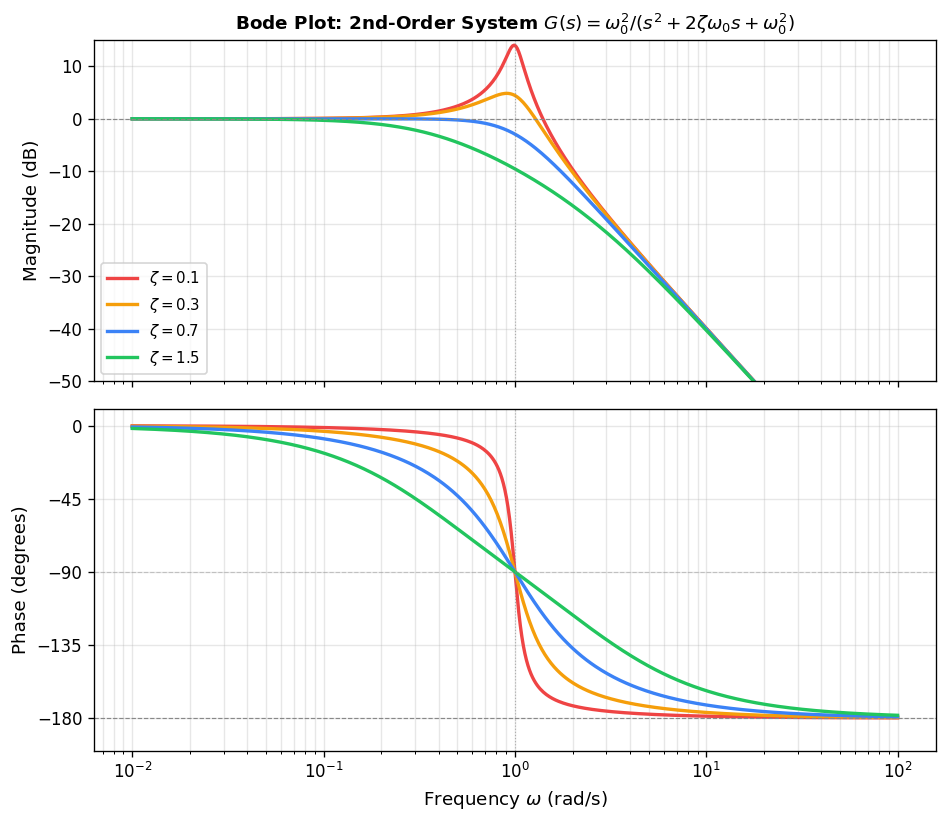
\[ G(s) = \frac{\omega_0^2}{s^2 + 2\zeta\omega_0 s + \omega_0^2}, \]where \( \omega_0 > 0 \) is the natural frequency and \( \zeta > 0 \) is the damping ratio. The gain and phase of the frequency response are
\[ \text{gain (dB)} = 40\log\omega_0 - 10\log\!\left(\omega^4 + 2\omega_0^2\omega^2(2\zeta^2 - 1) + \omega_0^4\right), \]\[ \text{phase (deg)} = -\frac{180^\circ}{\pi}\arctan\frac{2\zeta\omega_0\,\omega}{\omega_0^2 - \omega^2}. \]For \( \omega \ll \omega_0 \), the gain is approximately 0 dB and the phase approaches \( 0^\circ \). For \( \omega \gg \omega_0 \), the gain falls at \( -40 \) dB/decade and the phase approaches \( -180^\circ \). The transition near \( \omega = \omega_0 \) depends strongly on the damping ratio: for small \( \zeta \) (lightly damped systems), a sharp resonance peak appears in the gain curve near \( \omega_0 \), while large \( \zeta \) (heavily damped systems) produces a much smoother roll-off. The height of the resonance peak grows as \( \zeta \to 0 \), approaching infinity for an undamped system (which has poles on the imaginary axis at \( \pm j\omega_0 \). The higher the damping ratio, the flatter the Bode curves.
In MATLAB, for a defined transfer function object G, the command bode(G) generates the Bode plot automatically. For instance, to plot the Bode diagram for the second-order system with \( \omega_0 = 1 \) and \( \zeta = 0.1 \):
s = tf('s');
zeta = 0.1;
G = 1/(s^2 + 2*zeta*s + 1);
bode(G);
The resulting Bode plot shows the characteristic resonance peak in the gain curve near \( \omega = 1 \) rad/s and the transition in the phase curve from \( 0^\circ \) to \( -180^\circ \).
Poles, Zeros, and Internal Stability
Poles and Zeros
The input-output behavior of a linear control system is shaped, to a remarkable degree, by the locations of certain special points in the complex plane associated with its transfer function. These points — the poles and zeros — encode information about the system’s natural frequencies, resonances, and the signals it can block. In this lecture we define poles and zeros precisely, relate them to the underlying state-space realization, and examine their influence on the step response.
Poles and Zeros for a SISO Transfer Function
Definition 9.1 (Poles and zeros). Consider a SISO transfer function written in the coprime form
\[ G(s) = \frac{n(s)}{d(s)}, \]where \(n(s)\) and \(d(s)\) are coprime polynomials (i.e., their greatest common divisor is 1). The roots of the numerator \(n(s)\) are called the zeros of \(G(s)\), and the roots of the denominator \(d(s)\) are called the poles of \(G(s)\).
This definition parallels the notion of poles and zeros from complex analysis. Note that complex poles and zeros always appear in conjugate pairs when the coefficients of \(n(s)\) and \(d(s)\) are real.
Example 9.2. Consider
\[ G(s) = \frac{s+1}{s^2 + s + 1}. \]There is a single zero at \(s = -1\) and two poles at \(s = \frac{-1 \pm j\sqrt{3}}{2}\). Tools such as pzplot or pzmap in MATLAB render these graphically: poles are indicated by a cross (\(\times\) and zeros by a circle (\(\circ\).
Relationship with the Frequency Response
Any SISO transfer function can be factored as
\[ G(s) = k \frac{(s - z_1)(s - z_2)\cdots(s - z_r)}{(s - p_1)(s - p_2)\cdots(s - p_n)}, \]where \(z_1, \ldots, z_r\) are the zeros, \(p_1, \ldots, p_n\) are the poles, and \(k\) is a scalar gain. Evaluating on the imaginary axis at \(s = j\omega\) yields
\[ G(j\omega) = k \frac{(j\omega - z_1)(j\omega - z_2)\cdots(j\omega - z_r)}{(j\omega - p_1)(j\omega - p_2)\cdots(j\omega - p_n)}. \]Taking logarithms and arguments, we obtain
\[\begin{aligned} \log |G(j\omega)| &= \log k + \sum_{i=1}^{r} |j\omega - z_i| - \sum_{i=1}^{n} |j\omega - p_i|, \\ \angle G(j\omega) &= \sum_{i=1}^{r} \angle(j\omega - z_i) - \sum_{i=1}^{n} \angle(j\omega - p_i). \end{aligned}\]In other words, both the magnitude and phase of the frequency response are completely determined by the pole-zero locations up to an overall gain constant. The geometric interpretation — each term is the angle or distance from \(j\omega\) to a specific pole or zero in the complex plane — provides an intuitive way to reason about Bode plots without explicit computation.
Relationship with State-Space Realizations
Poles Versus Eigenvalues
Let \((A, B, C, D)\) be a state-space realization of \(G(s)\). Recall that
\[ G(s) = C(sI - A)^{-1}B + D = \frac{C\,\mathrm{adj}(sI - A)B + D\det(sI - A)}{\det(sI - A)} = \frac{n(s)}{d(s)}. \]It is possible for \(C\,\mathrm{adj}(sI-A)B + D\det(sI-A)\) and \(\det(sI-A)\) to share common factors, which must be cancelled to reach the coprime form. Nevertheless, every root of \(d(s)\) is always a root of \(\det(sI-A)\), the characteristic polynomial of \(A\). Hence every pole of \(G(s)\) is an eigenvalue of \(A\). The converse holds precisely when the realization is minimal.
Theorem 9.3. Let \((A, B, C, D)\) be a realization of a SISO transfer function \(G(s)\). Then every pole of \(G(s)\) is an eigenvalue of \(A\). Furthermore, the following statements are equivalent:
- All eigenvalues of \(A\) are poles of \(G(s)\).
- \((A, B, C, D)\) is a minimal realization of \(G(s)\).
- \(C\,\mathrm{adj}(sI-A)B\) and \(\det(sI-A)\) are coprime.
The proof follows from the observation that if \((A_1, B_1, C_1, D_1)\) is a minimal realization, then its denominator has strictly smaller degree than \(\det(sI-A)\) whenever \((A, B, C, D)\) is non-minimal, so \(\det(sI-A)\) and \(C\,\mathrm{adj}(sI-A)B\) cannot be coprime in that case.
Zeros Versus Invariant Zeros
Let \(u(t) = e^{st}u_0\) be an exponential input with \(u_0 \in \mathbb{R}\) and let \(s \neq \lambda(A)\) (i.e., \(s\) is not an eigenvalue of \(A\). A computation using the variation-of-parameters formula shows that if one chooses the initial condition \(x_0 = (sI - A)^{-1}Bu_0\), then
\[\begin{aligned} x(t) &= (sI - A)^{-1}B\,e^{st}u_0, \\ y(t) &= \bigl[C(sI-A)^{-1}B + D\bigr]e^{st}u_0 = G(s)\,e^{st}u_0. \end{aligned}\]If \(s\) is a zero of \(G(s)\), then \(y(t) = 0\) for all \(t \geq 0\): the system completely blocks the transmission of the exponential \(e^{st}\). Substituting \(x(t) = e^{st}x_0\) back into the state equations yields
\[ \begin{bmatrix} sI - A & -B \\ -C & -D \end{bmatrix} \begin{bmatrix} x_0 \\ u_0 \end{bmatrix} = 0, \]which has a nonzero solution only if the matrix on the left loses rank. This motivates the following definition.
Definition 9.4 (Invariant zeros). A complex number \(s\) is called an invariant zero of the state-space model \((A, B, C, D)\) if
\[ \mathrm{rank}\begin{bmatrix} sI - A & -B \\ -C & -D \end{bmatrix} < n + 1. \]Theorem 9.5. Let \((A, B, C, D)\) be a realization of a SISO transfer function \(G(s)\). Then every zero of \(G(s)\) is an invariant zero of \((A, B, C, D)\). Furthermore, the following statements are equivalent:
- All invariant zeros of \((A, B, C, D)\) are zeros of \(G(s)\).
- \((A, B, C, D)\) is a minimal realization of \(G(s)\).
- \(C\,\mathrm{adj}(sI-A)B\) and \(\det(sI-A)\) are coprime.
Proof. Let \(s\) be a zero of \(G(s)\), so that \(C\,\mathrm{adj}(sI-A)B + D\det(sI-A) = 0\). By Cramer’s rule one verifies that
\[ C\,\mathrm{adj}(sI-A)B + D\det(sI-A) = \det\begin{bmatrix} sI-A & -B \\ -C & -D \end{bmatrix}. \]Hence this determinant vanishes, meaning the matrix loses rank and \(s\) is an invariant zero. The remainder of the equivalences follows by an argument parallel to that for Theorem 9.3.
Proposition 9.6 (Transmission blocking). Consider a SISO system \((A, B, C, D)\) with transfer function \(G(s)\). Let \(s_0\) be an invariant zero of \((A, B, C, D)\) that is not an eigenvalue of \(A\). Then there exists a nonzero input of the form \(u(t) = e^{s_0 t}u_0\) and an initial condition \(x_0\) such that the corresponding output \(y(t) = 0\) for all \(t \geq 0\). In particular, the same conclusion holds for any zero of \(G(s)\).
Proof. Since \(s_0\) is an invariant zero, there exists a nonzero vector \((x_0, u_0) \in \mathbb{R}^{n+1}\) satisfying
\[ \begin{bmatrix} s_0 I - A & -B \\ -C & -D \end{bmatrix} \begin{bmatrix} x_0 \\ u_0 \end{bmatrix} = 0. \]Because \(s_0\) is not an eigenvalue of \(A\), we can write \(x_0 = (s_0 I - A)^{-1}Bu_0\); in particular \(u_0 \neq 0\). Setting \(x(t) = e^{s_0 t}x_0\) and \(u(t) = e^{s_0 t}u_0\), the condition \(s_0 x_0 = Ax_0 + Bu_0\) ensures \(x'(t) = Ax(t) + Bu(t)\), and the condition \(Cx_0 + Du_0 = 0\) gives \(y(t) = 0\) for all \(t \geq 0\).
Effects of Zeros and Poles on the Step Response
The unit step response is the output produced by the input \(u(t) = 1\) for \(t \geq 0\) and zero initial conditions. Its Laplace transform is \(\hat{u}(s) = 1/s\), so the step response in the frequency domain is \(\hat{y}(s) = G(s)/s\).
Example 9.7 (Step response of a first-order system). A general first-order strictly proper transfer function is
\[ G(s) = \frac{a_0}{s + b_0} = \frac{k}{\tau s + 1}, \]where \(k = a_0/b_0\) is the DC gain (also called the steady-state gain) and \(\tau = 1/b_0\) is the time constant. With a unit step input, \(\hat{y}(s) = k/(s(\tau s+1))\), and taking the inverse Laplace transform yields the step response
\[ y(t) = k\!\left[1 - e^{-t/\tau}\right], \quad t \geq 0. \]The system rises monotonically from zero to the steady state \(k\), reaching approximately \(63\%\) of its final value after one time constant.
Example 9.8 (Step response of a second-order system). Consider
\[ G(s) = k\frac{\omega_n^2}{s^2 + 2\zeta\omega_n s + \omega_n^2}, \]where \(k\) is the DC gain, \(\omega_n = \sqrt{b_0}\) is the natural frequency, and \(\zeta = b_1/(2\omega_n)\) is the damping ratio. In the underdamped case \(\zeta < 1\), the step response is
\[ y(t) = k\!\left[1 - \frac{1}{\beta}e^{-\zeta\omega_n t}\sin(\beta\omega_n t + \theta)\right], \]where \(\beta = \sqrt{1-\zeta^2}\) and \(\theta = \arctan(\beta/\zeta)\).
Adding a pole. Inserting an additional pole at location \(-a\) gives
\[ G_n(s) = \frac{ka\,\omega_n^2}{(s^2 + 2\zeta\omega_n s + \omega_n^2)(s+a)}, \]where the factor \(a\) in the numerator preserves the DC gain. Partial-fraction decomposition introduces an additional decaying exponential \(Ae^{-at}\) in the step response. If \(a\) is small (pole near the origin), this term dominates and slows the response considerably. As \(a\) grows large (pole far in the left half-plane), the term \(Ae^{-at}\) decays very rapidly and the original behavior is largely recovered. In general, adding a left-half-plane pole makes the step response slower, with the effect diminishing as the pole moves away from the origin.
Adding a zero. Inserting a zero at \(-a\) gives
\[ G_n(s) = k\frac{\omega_n^2(s + a)}{a(s^2 + 2\zeta\omega_n s + \omega_n^2)} = \left[\frac{s}{a} + 1\right]G(s). \]In the time domain the step response becomes
\[ y_n(t) = \frac{\dot{y}(t)}{a} + y(t), \]where \(y(t)\) is the original step response. Two cases arise. When \(a > 0\) (the zero lies in the left half-plane), the derivative contribution increases the overshoot and speeds up the response; larger \(a\) diminishes this effect. When \(a < 0\) (the zero lies in the right half-plane), the derivative contribution opposes the initial rise, reducing overshoot or even introducing an undershoot — a phenomenon in which the response initially moves in the wrong direction before ultimately settling. Right-half-plane zeros are often called non-minimum phase zeros and impose fundamental limitations on achievable closed-loop performance.
Internal Stability
From this lecture onward the focus turns from modeling to the analysis and design of control systems. The most fundamental property a control system must possess is stability: loosely, the assurance that trajectories do not grow without bound. Among the several stability notions in the literature, we study here internal stability, which concerns the free evolution of the state under no external input.
Definition of Internal Stability
Definition 10.9. An \(n \times n\) matrix \(A\) is said to be Hurwitz if \(\mathrm{Re}(\lambda) < 0\) for every eigenvalue \(\lambda\) of \(A\). Equivalently, all eigenvalues of \(A\) lie in the open left half of the complex plane, denoted \(\mathbb{C}^-\).
Definition 10.10. An LTI system \((A, B, C, D)\) is said to be internally stable if \(A\) is Hurwitz.
The terminology “internal” distinguishes this notion from input-output stability (which concerns whether bounded inputs produce bounded outputs) and from the stability of specific equilibria for nonlinear systems. For an unforced linear system \(x'= Ax\), the question reduces entirely to the spectral properties of \(A\).
Example 10.11. Consider the inverted pendulum, whose equations of motion linearized about the hanging equilibrium \((\pi, 0)\) are
\[ x' = \begin{bmatrix} 0 & 1 \\ -g/\ell & -b/(m\ell^2) \end{bmatrix} x + \begin{bmatrix} 0 \\ 1 \end{bmatrix} u, \quad y = \begin{bmatrix} 1 & 0 \end{bmatrix} x. \]The eigenvalues of the system matrix satisfy
\[ \lambda\!\left(\lambda + \frac{b}{m\ell^2}\right) + \frac{g}{\ell} = 0 \implies \lambda = -\frac{b}{2m\ell^2} \pm \sqrt{\left(\frac{b}{2m\ell^2}\right)^2 - \frac{g}{\ell}}. \]Both eigenvalues have negative real parts, so the hanging equilibrium is internally stable. In contrast, the linearization about the upright equilibrium \((0,0)\) has system matrix
\[ A = \begin{bmatrix} 0 & 1 \\ g/\ell & -b/(m\ell^2) \end{bmatrix}, \]with eigenvalues
\[ \lambda = -\frac{b}{2m\ell^2} \pm \sqrt{\left(\frac{b}{2m\ell^2}\right)^2 + \frac{g}{\ell}}. \]One eigenvalue has positive real part, confirming that the upright equilibrium is internally unstable and requires active control to stabilize.
The Internal Stability Theorem
The following central result provides four equivalent characterizations of internal stability, connecting the spectral condition on \(A\) to the long-run behavior of solutions and to the existence of a quadratic Lyapunov function.
Theorem 10.12 (Internal stability). The following statements are equivalent:
- \(A\) is Hurwitz (all eigenvalues have negative real parts).
- \(\lim_{t\to\infty} e^{At}x_0 = 0\) for all \(x_0 \in \mathbb{R}^n\).
- There exist constants \(M, c > 0\) such that \(\|x(t)\| \leq M e^{-ct}\|x_0\|\) for all \(t \geq 0\), where \(x(t) = e^{At}x_0\) solves \(x' = Ax\) with \(x(0) = x_0\).
- For every positive definite matrix \(Q\), there exists a unique positive definite matrix \(P\) satisfying the Lyapunov equation
Remark 10.13. Item (2) is called asymptotic stability and item (3) is called exponential stability. For unforced linear systems these two notions coincide, and both are equivalent to the existence of the quadratic Lyapunov function \(V(x) = x^T P x\) solving the Lyapunov equation in (4). The matrix \(P\) and the function \(V\) play a central role not only in linear analysis but also in the stability theory of nonlinear systems.
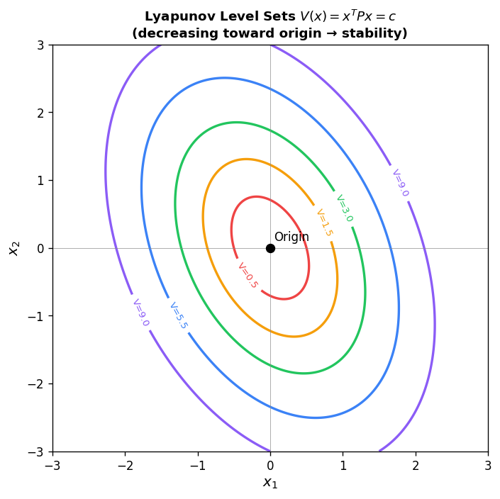
Proof (selected directions).
(1) \(\Rightarrow\) (3) \(\Rightarrow\) (2). Every entry of \(e^{At}\) is a linear combination of terms of the form \(e^{\alpha t}\cos\beta t\) and \(e^{\alpha t}\sin\beta t\), where \(\lambda = \alpha + j\beta\) is an eigenvalue of \(A\). Since all eigenvalues satisfy \(\alpha < 0\), these entries decay exponentially, giving (3) and then (2).
(4) \(\Rightarrow\) (2). Take \(Q = I\) and let \(V(x) = x^T Px\). Along any trajectory \(x(t)\) of \(x' = Ax\),
\[ \frac{dV(x(t))}{dt} = x^T(t)\bigl[A^T P + PA\bigr]x(t) = -\|x(t)\|^2 \leq 0. \]To convert this into decay of \(x(t)\) itself, we invoke the following lemma.
Lemma 10.14. If \(P \in \mathbb{R}^{n\times n}\) is positive definite, then
\[ \lambda_{\min}(P)\|x\|^2 \leq x^T Px \leq \lambda_{\max}(P)\|x\|^2, \quad \forall\, x \in \mathbb{R}^n, \]where \(\lambda_{\min}(P)\) and \(\lambda_{\max}(P)\) are the smallest and largest eigenvalues of \(P\).
Proof of Lemma. Since \(P\) is real symmetric it is orthogonally diagonalizable: there exists an orthogonal matrix \(W\) with \(W^T P W = \mathrm{diag}(\lambda_1, \ldots, \lambda_n)\) and all \(\lambda_i > 0\). Then
\[ x^T P x = (W^T x)^T \mathrm{diag}(\lambda_1,\ldots,\lambda_n)(W^T x) \leq \lambda_{\max}(P)\,\|W^Tx\|^2 = \lambda_{\max}(P)\|x\|^2, \]with the lower bound following similarly.
Using Lemma 10.14 in the Lyapunov derivative inequality gives
\[ \frac{dV(x(t))}{dt} = -\|x(t)\|^2 \leq -\frac{1}{\lambda_{\max}(P)} x^T(t)Px(t) = -\frac{1}{\lambda_{\max}(P)} V(x(t)). \]Hence
\[ \frac{d}{dt}\!\left[e^{t/\lambda_{\max}(P)} V(x(t))\right] \leq 0, \]so the quantity \(e^{t/\lambda_{\max}(P)}V(x(t))\) is non-increasing. This implies
\[ V(x(t)) \leq e^{-t/\lambda_{\max}(P)} V(x(0)), \quad \forall\, t \geq 0. \]Applying Lemma 10.14 once more yields
\[ \|x(t)\| \leq \sqrt{\frac{\lambda_{\max}(P)}{\lambda_{\min}(P)}}\,e^{-t/(2\lambda_{\max}(P))}\|x(0)\|, \]which establishes (3).
(2) \(\Rightarrow\) (1) (Sketch). Suppose some eigenvalue \(\lambda\) of \(A\) satisfies \(\mathrm{Re}(\lambda) \geq 0\). Then there exists \(x_0 \in \mathbb{R}^n\) such that \(e^{At}x_0\) does not tend to zero (since the corresponding Jordan block contributes a non-decaying term), contradicting (2).
(1) \(\Rightarrow\) (4). Define
\[ P = \int_0^\infty e^{A^T t} Q\, e^{At}\,dt. \]Since \(A\) is Hurwitz, the integrand decays exponentially and \(P\) is well-defined and positive definite. Differentiating under the integral,
\[\begin{aligned} A^T P + PA &= \int_0^\infty \frac{d}{dt}\!\left[e^{A^T t}Q\,e^{At}\right]dt \\ &= e^{A^T t}Q\,e^{At}\Big|_0^\infty = 0 - Q = -Q, \end{aligned}\]where the boundary term at infinity vanishes because \(A\) and \(A^T\) are both Hurwitz.
Stabilizability and Stabilization
Stabilizability
Having established what internal stability means, a natural question arises: if a system is not internally stable, can we design a control input to drive all trajectories to zero? This question is not always answerable in the affirmative — the answer depends on a structural property of the pair \((A, B)\) called stabilizability.
Definition and Basic Properties
Consider an LTI system \(x' = Ax + Bu\).
Definition 11.1. The system \((A, B)\) is said to be stabilizable if, for every initial state \(x_0 \in \mathbb{R}^n\), there exists a control input \(u: [0,\infty) \to \mathbb{R}^k\) such that
\[ \lim_{t\to\infty} x(t) = \lim_{t\to\infty}\!\left[e^{At}x_0 + \int_0^t e^{A(t-\tau)}Bu(\tau)\,d\tau\right] = 0. \]In other words, for every initial condition a control exists that asymptotically steers the state to the origin.
Proposition 11.2. The following hold:
- If \((A, B)\) is controllable, then \((A, B)\) is stabilizable, because controllability allows one to drive the state exactly to zero in finite time, after which the zero input keeps it there.
- If \(A\) is Hurwitz, then \((A, B)\) is stabilizable, because all trajectories decay to zero even under zero input.
- Stabilizability is invariant under state transformation: if \(P\) is nonsingular, then \((A, B)\) is stabilizable if and only if \((PAP^{-1}, PB)\) is stabilizable.
Equivalent Characterizations
The following theorem gives six equivalent ways to detect stabilizability, each illuminating a different facet of the concept.
Theorem 11.3 (Stabilizability). The following statements are equivalent:
- \((A, B)\) is stabilizable.
- The uncontrollable part \(A_u\) of \((A, B)\) (the matrix governing the uncontrollable modes in the Kalman decomposition, if it exists) is Hurwitz.
- (Stabilization by state feedback) There exists a matrix \(K \in \mathbb{R}^{k \times n}\) such that \(A + BK\) is Hurwitz.
- (PBH test) \(\mathrm{rank}[A - \lambda I \;\; B] = n\) for every complex number \(\lambda\) with \(\mathrm{Re}(\lambda) \geq 0\).
- (Eigenvector test) Every eigenvector of \(A^T\) corresponding to an eigenvalue \(\lambda\) with \(\mathrm{Re}(\lambda) \geq 0\) is not in the kernel of \(B^T\).
- (Lyapunov test) There exists a positive definite matrix \(P\) such that
Proof (selected directions).
(6) \(\Rightarrow\) (3). Let \(K = -\tfrac{1}{2}B^T P^{-1}\). Then
\[\begin{aligned} (A + BK)P + P(A + BK)^T &= \left(A - \tfrac{1}{2}BB^T P^{-1}\right)P + P\left(A - \tfrac{1}{2}BB^T P^{-1}\right)^T \\ &= AP + PA^T - BB^T < 0. \end{aligned}\]Left- and right-multiplying by \(Q = P^{-1}\) gives \(Q(A+BK) + (A+BK)^T Q < 0\), which by the Lyapunov characterization (Theorem 10.12, item (4)) shows that \(A + BK\) is Hurwitz.
(3) \(\Rightarrow\) (1). With the state feedback \(u(t) = Kx(t)\), the closed-loop system becomes \(x' = (A + BK)x\). Since \(A + BK\) is Hurwitz, all solutions decay exponentially to zero for any initial condition.
(4) \(\Rightarrow\) (5). Suppose there is a left eigenvector \(v \neq 0\) of \(A^T\) for an unstable eigenvalue \(\lambda\) (meaning \(\mathrm{Re}(\lambda) \geq 0\) with \(B^T v = 0\). Then
\[ \begin{bmatrix} B^T \\ A^T - \lambda I \end{bmatrix} v = 0, \]so the matrix has less than full column rank, and after transposing, \([A - \lambda I \;\; B]\) fails to have full row rank, violating (4).
(5) \(\Rightarrow\) (4). Essentially the reverse of the argument above.
(2) \(\Rightarrow\) (5). If no uncontrollable part exists, \((A,B)\) is controllable and the eigenvector test for controllability yields the conclusion. Otherwise, via a nonsingular transformation \(P\), write
\[ PAP^{-1} = \begin{bmatrix} A_c & A_{12} \\ 0 & A_u \end{bmatrix}, \quad PB = \begin{bmatrix} B_c \\ 0 \end{bmatrix}. \]Suppose for contradiction that \(A^T\) has an eigenvector \(v\) in \(\ker(B^T)\) for an unstable eigenvalue \(\lambda\). Translating via \((P^T)^{-1}\), one finds that the lower block component \(v_u \neq 0\) and \(A_u^T v_u = \lambda v_u\), giving \(\lambda\) as an eigenvalue of \(A_u\) with \(\mathrm{Re}(\lambda) \geq 0\), contradicting that \(A_u\) is Hurwitz.
(1) \(\Rightarrow\) (2). If \(A_u\) exists and is not Hurwitz, the coordinate change \(z = Px\) decouples the uncontrollable subsystem \(z_2' = A_u z_2\). Since \(A_u\) is not Hurwitz, \(z_2\) cannot be driven to zero, and hence \((A, B)\) is not stabilizable.
(4) \(\Rightarrow\) (2). If \(A_u\) is not Hurwitz, pick an unstable eigenvalue \(\lambda\) of \(A_u^T\) with eigenvector \(v\). Setting \(w = [0 \;\; v^T]\) and computing \(w[PAP^{-1} - \lambda I \;\; PB]\) gives the zero row vector, so \(wP[A - \lambda I \;\; B] = 0\) with \(wP \neq 0\), and \(\mathrm{rank}[A - \lambda I \;\; B] < n\).
The proof of (2) \(\Rightarrow\) (6) is deferred to Lecture 12, where it follows from the Lyapunov test for controllability.
Example 11.4. Consider the system
\[ x' = \begin{bmatrix} 1 & -1 \\ 0 & -1 \end{bmatrix} x + \begin{bmatrix} 1 \\ 0 \end{bmatrix} u. \]The controllability matrix is \(\begin{bmatrix}1 & 1 \\ 0 & 0\end{bmatrix}\), which has rank 1 < 2, so the system is not controllable. However, a controllable decomposition reveals the uncontrollable part \(A_u = -1\), which is Hurwitz, so the system is stabilizable by statement (2) of Theorem 11.3.
Verification via the PBH test: the eigenvalues of \(A\) are \(\pm 1\). The only unstable eigenvalue is \(\lambda = 1\), and
\[ [A - I \;\; B] = \begin{bmatrix} 0 & -1 & 1 \\ 0 & 1 & 0 \end{bmatrix} \]has rank 2 = n, confirming stabilizability.
For a direct construction, let \(K = [k_1 \;\; k_2]\). Then
\[ A + BK = \begin{bmatrix} 1+k_1 & -1+k_2 \\ 0 & -1 \end{bmatrix}. \]Choosing \(k_1 < -1\) makes both diagonal entries negative, rendering \(A + BK\) Hurwitz. Notice that the uncontrollable eigenvalue \(-1\) cannot be altered by state feedback, but since it is already stable, stabilization is achievable.
Stabilization of Controllable Systems
Theorem 11.3 tells us that a stabilizable system can be stabilized by a state feedback \(u = Kx\) making \(A + BK\) Hurwitz. For controllable systems, a much stronger result holds: not only can the closed-loop matrix be made Hurwitz, but its eigenvalues can be placed anywhere in the complex plane (subject to the conjugate-pair constraint). This lecture establishes that claim and provides a constructive proof via the controllable canonical form.
Lyapunov Tests for Controllability and Stabilizability
Before reaching the main theorem, we establish two Lyapunov-based characterizations that complete the proof of Theorem 11.3 and prepare the ground for eigenvalue placement.
Proposition 12.5 (Eigenvalue test for controllability). The pair \((A, B)\) is controllable if and only if no eigenvector of \(A^T\) lies in the kernel of \(B^T)\).
Proof. Suppose some eigenvector \(v \neq 0\) of \(A^T\) satisfies \(B^T v = 0\) and \(A^T v = \lambda v\). Then
\[ \begin{bmatrix} B^T \\ A^T - \lambda I \end{bmatrix} v = 0, \]so this matrix lacks full column rank; transposing, \([A - \lambda I \;\; B]\) lacks full row rank, and by the PBH test \((A, B)\) is uncontrollable. The “if” direction follows by reversing the argument.
Proposition 12.6 (Lyapunov test for controllability). Suppose \(A\) is Hurwitz. The pair \((A, B)\) is controllable if and only if there exists a unique positive definite solution \(W\) to the Lyapunov equation
\[ AW + WA^T = -BB^T. \]Proof. (\(\Rightarrow\) Define
\[ W = \int_0^\infty e^{A\tau} BB^T e^{A^T\tau}\,d\tau. \]Since \(A\) is Hurwitz the integral converges. Controllability of \((A, B)\) ensures \(W\) is positive definite (it is the controllability Gramian). A computation analogous to the proof of Theorem 10.12 shows \(AW + WA^T = -BB^T\). For uniqueness, suppose \(\hat{W}\) also satisfies the equation. Then \(A(W - \hat{W}) + (W-\hat{W})A^T = 0\). Left- and right-multiplying by \(e^{At}\) and \(e^{A^T t}\) shows that \(e^{At}(W - \hat{W})e^{A^T t}\) is constant in \(t\); since both \(A\) and \(A^T\) are Hurwitz this expression tends to zero as \(t \to \infty\), forcing it to be identically zero; at \(t = 0\) we get \(W = \hat{W}\).
(\(\Leftarrow\) Let \(v\) be an eigenvector of \(A^T\) with eigenvalue \(\lambda\). Then
\[ v^*(AW + WA^T)v = 2\,\mathrm{Re}(\lambda)\,v^*Wv = -\|B^Tv\|^2. \]Since \(W\) is positive definite, \(v^*Wv > 0\). Hence \(\|B^Tv\|^2 > 0\), i.e., \(v \notin \ker(B^T)\). By Proposition 12.5, \((A, B)\) is controllable.
Stabilization with Arbitrary Decay Rate
Theorem 12.7 (Stabilization by state feedback for controllable systems). The following statements are equivalent:
- \((A, B)\) is controllable.
- For every \(\mu > 0\), there exists a matrix \(K\) such that \(A + BK\) is Hurwitz and \(\mathrm{Re}(\lambda) \leq -\mu\) for all eigenvalues \(\lambda\) of \(A + BK\).
Proof. (\(\Rightarrow\) Since eigenvectors of \(A^T\) and \(-\mu I - A^T\) are in bijection (via \(A^T v = \lambda v \Leftrightarrow (-\mu I - A^T)v = -(\mu+\lambda)v\), the pair \((A, B)\) is controllable if and only if \((-\mu I - A, B)\) is controllable for any \(\mu \in \mathbb{R}\). Choose \(\mu\) large enough that \(-\mu I - A\) is Hurwitz. By the Lyapunov test for controllability, there exists a positive definite \(W\) such that
\[ W(-\mu I - A)^T + (-\mu I - A)W = -BB^T, \tag{12.1} \]which simplifies to
\[ AW + WA^T - BB^T = -2\mu W. \]Setting \(P = W^{-1}\) and multiplying through, this becomes
\[ P(A + BK) + (A + BK)^T P = -2\mu P, \quad K = -\tfrac{1}{2}B^T P. \]The quadratic Lyapunov function \(V(x) = x^T P x\) then satisfies \(V(x(t)) = V(x(0))e^{-2\mu t}\), so \(\|x(t)\|\) decays at rate \(\mu\) and all eigenvalues of \(A + BK\) have real part at most \(-\mu\).
(\(\Leftarrow\) If \((A, B)\) is not controllable, a coordinate transformation gives the decomposed form
\[ PAP^{-1} = \begin{bmatrix} A_c & A_{12} \\ 0 & A_u \end{bmatrix}, \quad PB = \begin{bmatrix} B_c \\ 0 \end{bmatrix}. \]For any \(K\), the closed-loop matrix in the new coordinates is
\[ P(A+BK)P^{-1} = \begin{bmatrix} A_c + B_c K_1 & A_{12} + B_c K_2 \\ 0 & A_u \end{bmatrix}, \]which is block upper triangular with \(A_u\) unchanged in the lower-right corner. The eigenvalues of \(A_u\) remain eigenvalues of \(A + BK\) and cannot be shifted, so statement (2) fails.
The Lyapunov Test for Stabilizability (Completing Theorem 11.3)
Corollary 12.8 (Lyapunov test for stabilizability). The pair \((A, B)\) is stabilizable if and only if there exists a positive definite matrix \(P\) such that
\[ AP + PA^T - BB^T < 0. \]Proof. The “if” direction is the implication (6) \(\Rightarrow\) (3) in Theorem 11.3. For the “only if” direction, suppose \((A, B)\) is stabilizable. If it is also controllable, equation (12.1) gives a positive definite \(W\) satisfying \(AW + WA^T - BB^T = -2\mu W < 0\). If it is not controllable, the Kalman decomposition gives controllable pair \((A_c, B_c)\) and Hurwitz uncontrollable part \(A_u\). Let \(W_c > 0\) satisfy \(A_c W_c + W_c A_c^T - B_c B_c^T = -2\mu W_c\), and let \(W_u > 0\) satisfy \(W_u A_u^T + A_u W_u = -I\) (by the Lyapunov stability test for \(A_u\). Set
\[ W = \begin{bmatrix} W_c & 0 \\ 0 & \rho W_u \end{bmatrix}. \]Then
\[ A_1 W + WA_1^T - B_1 B_1^T = \begin{bmatrix} -2\mu W_c & \rho A_{12}W_u \\ \rho W_u A_{12}^T & -\rho I \end{bmatrix}, \]where \(A_1 = PAP^{-1}\) and \(B_1 = PB\). For \(\rho > 0\) chosen sufficiently small (completing the square in the off-diagonal blocks shows this is feasible), the right-hand side is negative definite, completing the proof.
Eigenvalue Assignment by State Feedback
Theorem 12.7 guarantees that a controllable system can be stabilized with eigenvalues pushed as far left as desired. The following theorem sharpens this to full freedom of eigenvalue placement.
Theorem 12.9 (Eigenvalue assignment by state feedback for controllable systems). The following statements are equivalent:
- The pair \((A, B)\) is controllable.
- For every set of complex numbers \(\{\lambda_1, \lambda_2, \ldots, \lambda_n\}\) in which complex values appear in conjugate pairs, there exists a matrix \(K \in \mathbb{R}^{k \times n}\) such that the eigenvalues of \(A + BK\) are exactly \(\{\lambda_1, \ldots, \lambda_n\}\).
This is the pole placement theorem, one of the foundational results of linear control theory. The condition that complex eigenvalues appear in conjugate pairs is required to ensure \(K\) is real.
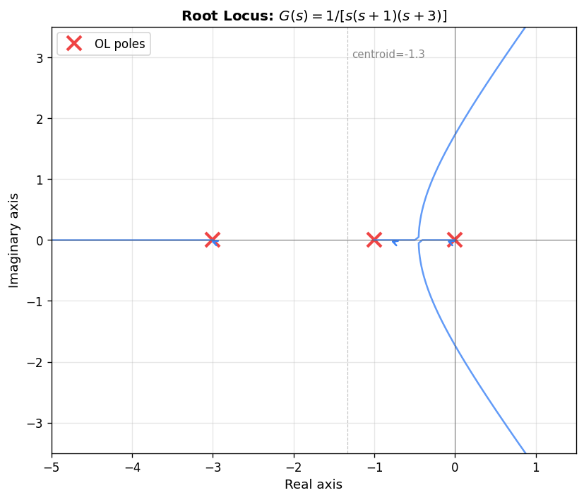
Proof. (2) \(\Rightarrow\) (1) follows from the same argument as the converse direction in Theorem 12.7: uncontrollable eigenvalues are immune to state feedback.
For (1) \(\Rightarrow\) (2), we prove the single-input case. The multi-input case is in [AM06]. The proof uses the controllable canonical form.
Lemma 12.10 (Controllable canonical form). If \((A, B)\) is controllable (with \(B \in \mathbb{R}^{n\times 1}\), there exists a nonsingular matrix \(P\) such that
\[ PAP^{-1} = \begin{bmatrix} 0 & 1 & 0 & \cdots & 0 \\ 0 & 0 & 1 & \cdots & 0 \\ \vdots & \vdots & \vdots & \ddots & \vdots \\ 0 & 0 & 0 & \cdots & 1 \\ -b_0 & -b_1 & -b_2 & \cdots & -b_{n-1} \end{bmatrix}, \quad PB = \begin{bmatrix} 0 \\ \vdots \\ 0 \\ 1 \end{bmatrix}, \]where \(b_0, b_1, \ldots, b_{n-1}\) are the coefficients of the characteristic polynomial
\[ \det(sI - A) = b_0 + b_1 s + \cdots + b_{n-1}s^{n-1} + s^n. \]Proof of Lemma. Since \((A, B)\) is controllable, the columns of the controllability matrix \([B \;\; AB \;\; A^2 B \;\; \cdots \;\; A^{n-1}B]\) are linearly independent and form a square invertible matrix. Define new basis vectors
\[\begin{aligned} v_n &= B, \\ v_{n-1} &= Av_n + b_{n-1}v_n = AB + b_{n-1}B, \\ v_{n-2} &= Av_{n-1} + b_{n-2}v_n = A^2B + b_{n-1}AB + b_{n-2}B, \\ &\vdots \\ v_1 &= Av_2 + b_1 v_n = A^{n-1}B + b_{n-1}A^{n-2}B + \cdots + b_1 B. \end{aligned}\]These vectors \(\{v_1, \ldots, v_n\}\) are linearly independent because they are related to \(\{B, AB, \ldots, A^{n-1}B\}\) by a triangular change of basis. Setting \(P^{-1} = [v_1 \;\; v_2 \;\; \cdots \;\; v_n]\), one has \(PB = e_n\) (the last standard basis vector). For \(PAP^{-1}\), the Cayley-Hamilton theorem gives \(A^n B = -b_0 B - b_1 AB - \cdots - b_{n-1}A^{n-1}B\), from which
\[\begin{aligned} Av_1 &= -b_0 v_n, \\ Av_2 &= v_1 - b_1 v_n, \\ &\vdots \\ Av_n &= v_{n-1} - b_{n-1}v_n, \end{aligned}\]yielding exactly the companion matrix form above.
Completion of proof of Theorem 12.9. In the canonical coordinates, with \(\hat{K} = [\hat{k}_0 \;\; \hat{k}_1 \;\; \cdots \;\; \hat{k}_{n-1}]\), the matrix \(PAP^{-1} + PB\hat{K}\) is again companion-form with last row \([-b_0 + \hat{k}_0, \; -b_1 + \hat{k}_1, \; \ldots, \; -b_{n-1}+\hat{k}_{n-1}]\), so its characteristic polynomial is
\[ s^n + (b_{n-1} - \hat{k}_{n-1})s^{n-1} + \cdots + (b_1 - \hat{k}_1)s + (b_0 - \hat{k}_0). \]Given any target polynomial \((s - \lambda_1)(s-\lambda_2)\cdots(s-\lambda_n) = s^n + a_{n-1}s^{n-1} + \cdots + a_1 s + a_0\), we simply choose \(\hat{k}_i = b_i - a_i\) for each \(i\). Setting \(K = \hat{K}P\) gives \(P(A+BK)P^{-1} = PAP^{-1} + PB\hat{K}\), so \(A + BK\) has the desired eigenvalues.
Example 12.11. Let
\[ A = \begin{bmatrix} 0 & 1 & 0 \\ 0 & 0 & 1 \\ 1 & 2 & 3 \end{bmatrix}, \quad B = \begin{bmatrix} 0 \\ 0 \\ 1 \end{bmatrix}. \]We want the eigenvalues of \(A + BK\) to be \(-1, -2\pm j\). The target characteristic polynomial is
\[ (\lambda+1)(\lambda+2-j)(\lambda+2+j) = \lambda^3 + 5\lambda^2 + 9\lambda + 5. \]Since \(A\) is already in controllable canonical form with coefficients \(b_0 = -1, b_1 = -2, b_2 = -3\) (note the signs from the last row \([1, 2, 3]\), setting \(K = [k_0 \;\; k_1 \;\; k_2]\) gives
\[ A + BK = \begin{bmatrix} 0 & 1 & 0 \\ 0 & 0 & 1 \\ 1+k_0 & 2+k_1 & 3+k_2 \end{bmatrix} \]with characteristic polynomial \(\lambda^3 - (3+k_2)\lambda^2 - (2+k_1)\lambda - (1+k_0)\). Matching coefficients:
\[ 1 + k_0 = -5, \quad 2 + k_1 = -9, \quad 3 + k_2 = -5, \]giving \(k_0 = -6, \; k_1 = -11, \; k_2 = -8\).
Example 12.12. Let
\[ A = \begin{bmatrix} 0 & 1 & 1 \\ 1 & 5 & 2 \\ -1 & -4 & -2 \end{bmatrix}, \quad B = \begin{bmatrix} 0 \\ 1 \\ -1 \end{bmatrix}. \]Again targeting eigenvalues \(-1, -2 \pm j\) with characteristic polynomial \(\lambda^3 + 5\lambda^2 + 9\lambda + 5\), with \(K = [k_0 \;\; k_1 \;\; k_2]\) one computes
\[ \det(\lambda I - (A + BK)) = \lambda^3 + (k_2 - k_1 - 3)\lambda^2 + (-k_2 - 2)\lambda + (-k_0 - 1). \]Matching gives \(k_0 = -6, \; k_1 = -19, \; k_2 = -11\).
Remark 12.13. For SISO systems, the gain matrix \(K\) for eigenvalue assignment is uniquely determined. In some textbooks the state feedback is written as \(u = -Kx\) rather than \(u = Kx\), leading to the closed-loop matrix \(A - BK\) instead of \(A + BK\). These are purely notational conventions and completely equivalent in content. Be aware that MATLAB’s place(A, B, P) command uses the convention \(A - BK\) and returns \(K\) such that \(A - BK\) has eigenvalues listed in the vector P.
Detectability and External Stability
Detectability and Stabilization by Output Feedback
In previous lectures we examined how state feedback of the form \( u = Kx \) can be used to stabilize a linear time-invariant (LTI) system. In many practical situations, however, it is impossible or prohibitively expensive to measure the full state vector. This lecture addresses how stabilization can still be achieved when only the output \( y \) is accessible, by coupling a state estimator — called an observer — with a state-feedback controller.
Observers and the Estimation Error
Suppose the governing state equation is \( x'(t) = Ax(t) + Bu(t) \) and we use it directly to build a copy of the dynamics:
\[ \hat{x}' = A\hat{x} + Bu. \tag{13.1} \]This system, driven by the same input \( u \) but without correction from observations, is the simplest state observer (or state estimator). To assess how well \( \hat{x} \) tracks the true state, define the estimation error
\[ e = \hat{x} - x. \tag{13.2} \]Differentiating and substituting the state equation yields
\[ e' = \hat{x}' - x' = A\hat{x} + Bu - (Ax + Bu) = A(\hat{x} - x) = Ae. \]If \( A \) is Hurwitz, then \( e(t) \to 0 \) as \( t \to \infty \), and the observer provides an asymptotically accurate estimate of the true state. When \( A \) is not Hurwitz, however, this open-loop observer fails to converge.
To remedy this, we exploit the measured output. Let \( y = Cx + Du \) be the observed output and \( \hat{y} = C\hat{x} + Du \) the output predicted by the estimator. The discrepancy \( \hat{y} - y \) is fed back to correct the estimator:
\[ \hat{x}' = A\hat{x} + Bu + L(\hat{y} - y), \tag{13.3} \]where \( L \) is the observer gain matrix, to be designed. Because \( \hat{y} - y = C\hat{x} - Cx = Ce \), the error dynamics become
\[ e' = \hat{x}' - x' = A\hat{x} + Bu + L(\hat{y} - y) - (Ax + Bu) = (A + LC)e. \tag{13.4} \]The estimation error converges to zero asymptotically if and only if \( A + LC \) is Hurwitz. The central question is therefore: can we find a matrix \( L \) such that \( A + LC \) has all eigenvalues strictly in the open left-half plane?
Detectability
This question is precisely the dual of stabilizability. Recall that \( (A, B) \) is stabilizable if and only if there exists a matrix \( K \) such that \( A + BK \) is Hurwitz. By analogy we make the following definition.
Definition 13.1 (Detectability). We call \( (A, C) \) detectable if there exists some matrix \( L \) such that \( A + LC \) is Hurwitz.
The precise duality between stabilizability and detectability is captured in the next result.
Proposition 13.2. The pair \( (A, B) \) is stabilizable if and only if \( (A^T, B^T) \) is detectable.
Proof. The pair \( (A, B) \) is stabilizable if and only if there exists a matrix \( K \) such that \( A + BK \) is Hurwitz. Since a matrix is Hurwitz if and only if its transpose is Hurwitz, \( A + BK \) is Hurwitz if and only if \( A^T + K^T B^T \) is Hurwitz. Setting \( L = K^T \) shows this is precisely the definition of \( (A^T, B^T) \) being detectable. \( \square \)
This duality immediately transfers the algebraic characterizations of stabilizability to detectability.
Theorem 13.3 (Detectability). The following statements are equivalent:
- \( (A, C) \) is detectable.
- The unobservable part \( A_u \) of the system (if it exists) is Hurwitz.
- (PBH test) For every complex number \( \lambda \) with \( \mathrm{Re}(\lambda) \geq 0 \),
The equivalence of these conditions follows by duality from the corresponding characterizations of stabilizability (via the PBH test and the Kalman decomposition). Condition 2 says that any mode which cannot be observed must at least be stable on its own. Condition 3 says that the only modes that can be “hidden” from the output — those for which the rank drops — must lie in the stable left-half plane.
Stabilization by Output Feedback
With an observer in hand, we can construct a state-feedback law that uses the estimated state in place of the true state. Set
\[ u = K\hat{x}, \tag{13.5} \]where \( \hat{x} \) is generated by the observer (13.3). Substituting into the state equation and writing \( \hat{x} = x + e \) gives
\[ x' = Ax + Bu = Ax + BK\hat{x} = Ax + BK(x + e) = (A + BK)x + BKe. \]Combining this with the error dynamics \( e' = (A + LC)e \) from (13.4), the closed-loop system is
\[\begin{align} \begin{bmatrix} x' \\ e' \end{bmatrix} = \begin{bmatrix} A + BK & BK \\ 0 & A + LC \end{bmatrix} \begin{bmatrix} x \\ e \end{bmatrix}. \tag{13.6} \end{align}\]Because the closed-loop matrix is block upper triangular, its characteristic polynomial factors as the product of the characteristic polynomials of the two diagonal blocks. This observation is the content of the following fundamental theorem.
Theorem 13.4 (Separation Principle). The closed-loop system (13.6) has characteristic polynomial
\[ \lambda(s) = \det(sI - (A + BK)) \cdot \det(sI - (A + LC)). \]Consequently, the eigenvalues of the closed-loop system are precisely the union of the eigenvalues of \( A + BK \) (determined by the state-feedback gain \( K \) and the eigenvalues of \( A + LC \) (determined by the observer gain \( L \). The separation principle allows the controller design and the observer design to be carried out independently.
Corollary 13.5 (Stabilization by Output Feedback). If \( (A, B) \) is stabilizable and \( (A, C) \) is detectable, then the output feedback law (13.5) with the observer (13.3) stabilizes the system.
Under the stronger assumption of full controllability and observability, eigenvalue placement is entirely free.
Theorem 13.6 (Eigenvalue Assignment by Output Feedback). If \( (A, B) \) is controllable and \( (A, C) \) is observable, then any desired characteristic polynomial for the closed-loop system (13.6) can be achieved by appropriate choice of the gain matrices \( K \) and \( L \).
Example 13.7. Consider the double-integrator system
\[ x' = \begin{bmatrix} 0 & 1 \\ 0 & 0 \end{bmatrix} x + \begin{bmatrix} 0 \\ 1 \end{bmatrix} u, \qquad y = \begin{bmatrix} 1 & 0 \end{bmatrix} x. \tag{13.7, 13.8} \]The controllability matrix is \( \begin{bmatrix} B & AB \end{bmatrix} = \begin{bmatrix} 0 & 1 \\ 1 & 0 \end{bmatrix} \), which has rank 2, so the system is controllable. The observability matrix is \( \begin{bmatrix} C \\ CA \end{bmatrix} = \begin{bmatrix} 1 & 0 \\ 0 & 1 \end{bmatrix} \), which also has rank 2, so the system is observable.
To illustrate the design procedure, choose \( L = \begin{bmatrix} \ell_1 \\ \ell_2 \end{bmatrix} \). Then
\[ A + LC = \begin{bmatrix} \ell_1 & 1 \\ \ell_2 & 0 \end{bmatrix}, \]with characteristic polynomial \( s^2 - \ell_1 s - \ell_2 \). By choosing \( \ell_1 \) and \( \ell_2 \) appropriately, any degree-2 polynomial can be achieved. Similarly, with \( K = \begin{bmatrix} k_1 & k_2 \end{bmatrix} \),
\[ A + BK = \begin{bmatrix} 0 & 1 \\ k_1 & k_2 \end{bmatrix}, \]with characteristic polynomial \( s^2 - k_2 s - k_1 \). Again any desired polynomial is achievable. The closed-loop system resulting from this procedure is called observer-based dynamic output feedback, because the output is processed via a dynamic state estimator rather than fed back directly.
Static Output Feedback
A natural follow-up question is whether one can dispense with the dynamic observer entirely and use a static output feedback law \( u = KCx \), seeking a gain \( K \) such that \( A + BKC \) is Hurwitz. Remarkably, this question — known as the stabilization by static output feedback problem — remains one of the fundamental open problems in control theory. Its difficulty is believed to be rooted in deep combinatorial complexity; in particular, pole placement via static output feedback has been shown to be NP-hard in general.
External Stability
The preceding lectures established a theory of internal stability: conditions on the system matrix \( A \) (or the poles of the state-space realization) that guarantee the free response decays to zero. We now turn to external stability, also called input-output stability, which characterizes how the magnitude of the output signal is bounded relative to the magnitude of the input signal when the initial conditions are set to zero. An externally stable system produces well-behaved outputs for all well-behaved inputs.
Signal Norms and \( L^p \) Spaces
To make precise what “well-behaved” means, we assign norms to signals. First recall that the \( p \)-norm of a vector \( x \in \mathbb{R}^k \) is
Definition 14.8. For \( p \geq 1 \), the \( p \)-norm of a vector \( x \in \mathbb{R}^k \) is
\[ \|x\|_p = \left( \sum_{i=1}^k |x_i|^p \right)^{1/p}. \]The case \( p = 2 \) is the Euclidean norm, written simply as \( \|x\| \). The infinity norm (or maximum norm) is
\[ \|x\|_\infty = \max_{1 \leq i \leq k} |x_i|. \]These vector norms extend to signal norms for functions \( u : [0,\infty) \to \mathbb{R}^k \).
Definition 14.9. Let \( u : [0,\infty) \to \mathbb{R}^k \). Define
\[\begin{aligned} \|u\|_\infty &= \sup_{t \geq 0} \|u(t)\|_\infty = \sup_{t \geq 0} \max_{1 \leq i \leq k} |u_i(t)|, \\[6pt] \|u\|_2 &= \sqrt{\int_0^\infty \|u(t)\|_2^2\, dt} = \sqrt{\int_0^\infty u^T(t)u(t)\, dt}, \\[6pt] \|u\|_1 &= \int_0^\infty \|u(t)\|_1\, dt = \int_0^\infty \sum_{i=1}^k |u_i(t)|\, dt. \end{aligned}\]More generally, for \( 1 \leq p < \infty \),
\[ \|u\|_p = \left( \int_0^\infty \|u(t)\|_p^p\, dt \right)^{1/p} = \left( \int_0^\infty \sum_{i=1}^k |u_i(t)|^p\, dt \right)^{1/p}. \]The signal space \( L^p[0,\infty) \) consists of all signals with finite \( \|\cdot\|_p \).
Definition 14.10 (\( L^p \)-stability). An LTI system is \( L^p \)-stable if there exists a constant \( \gamma \) such that
\[ \|y\|_p \leq \gamma \|u\|_p \]for all input-output pairs \( u, y \) with zero initial condition.
Remark 14.11. The constant \( \gamma \) is an upper bound on the \( L^p \)-gain of the system; the gain itself is the infimum of all such constants. For finite-dimensional LTI systems, all notions of \( L^p \)-stability (for different \( p \) turn out to be equivalent, although the corresponding gains may differ.
BIBO Stability
Because all \( L^p \)-stability notions are equivalent for LTI systems, we focus on the case \( p = \infty \), which yields bounded-input, bounded-output (BIBO) stability. A system is BIBO stable if every bounded input produces a bounded output (from zero initial conditions). The terminology “input-output stability” and “external stability” are used interchangeably with BIBO stability throughout this course.
Time-Domain Conditions for BIBO Stability
Recall that the zero-state output is given by the convolution
\[ y(t) = \int_0^t g(t - \tau) u(\tau)\, d\tau, \]where the impulse response is
\[ g(t) = Ce^{At}B + D\delta(t). \]Theorem 14.12. The LTI system \( (A, B, C, D) \) is BIBO stable if and only if every entry of \( g(t) \) is absolutely integrable, i.e.,
\[ \int_0^\infty |g_{ij}(t)|\, dt < \infty \]for all \( 1 \leq i \leq m \) and \( 1 \leq j \leq k \).
Proof. (\( \Leftarrow \) Suppose each entry of \( g \) is absolutely integrable. Then
\[\begin{aligned} \|y(t)\|_\infty &= \left\| \int_0^t g(t-\tau) u(\tau)\, d\tau \right\|_\infty \\ &= \max_{1 \leq i \leq m} \left| \int_0^t \sum_{j=1}^k g_{ij}(t-\tau) u_j(\tau)\, d\tau \right| \\ &\leq \max_{1 \leq i \leq m} \int_0^t \sum_{j=1}^k |g_{ij}(t-\tau)|\, |u_j(\tau)|\, d\tau \\ &\leq \max_{1 \leq i \leq m} \int_0^t \sum_{j=1}^k |g_{ij}(t-\tau)|\, d\tau \cdot \sup_{\tau \geq 0} \max_{1 \leq j \leq k} |u_j(\tau)| \\ &\leq \max_{1 \leq i \leq m} \sum_{j=1}^k \int_0^\infty |g_{ij}(\tau)|\, d\tau \cdot \|u\|_\infty. \end{aligned}\]Setting \( \gamma = \max_{1 \leq i \leq m} \sum_{j=1}^k \int_0^\infty |g_{ij}(t)|\, dt \), which is finite by assumption, we obtain \( \|y\|_\infty \leq \gamma \|u\|_\infty \), so the system is BIBO stable.
(\( \Rightarrow \) Suppose instead that \( \int_0^\infty |g_{ij}(t)|\, dt \) diverges for some indices \( i, j \). Then for each \( M > 0 \) there exists \( t > 0 \) such that \( \int_0^t |g_{ij}(\tau)|\, d\tau > M \). Fix such a \( t \) and define the bounded input
\[ u(\tau) = \begin{cases} e_j & \text{if } g_{ij}(t-\tau) \geq 0, \\ -e_j & \text{if } g_{ij}(t-\tau) < 0, \end{cases} \]where \( e_j \) is the standard basis vector in \( \mathbb{R}^k \) with 1 in position \( j \). Then the \( i \)-th component of the output satisfies \( y_i(t) = \int_0^t |g_{ij}(\tau)|\, d\tau > M \). Setting \( u(\tau) = 0 \) for \( \tau \geq t \) gives \( \|u\|_\infty = 1 \) yet \( \|y\|_\infty > M \). Since \( M \) is arbitrary, the system is not BIBO stable. \( \square \)
Remark 14.13. Suppose the system is BIBO stable, so \( \gamma = \max_{1 \leq i \leq m} \sum_{j=1}^k \int_0^\infty |g_{ij}(t)|\, dt < \infty \). For any \( \varepsilon > 0 \), one can construct an input with \( \|u\|_\infty = 1 \) such that \( \|y\|_\infty > \gamma - \varepsilon \), by choosing input signs to align with the sign of each \( g_{ij} \) entry. This shows that \( \gamma \) as defined is exactly the \( L^\infty \)-gain of the system — the smallest constant for which \( \|y\|_\infty \leq \gamma \|u\|_\infty \) holds.
Corollary 14.14. If \( A \) is Hurwitz (i.e., the system is internally stable), then the system is BIBO stable.
Proof. Since \( g(t) = Ce^{At}B + D\delta(t) \) and \( A \) Hurwitz implies the entries of \( e^{At} \) decay exponentially, each entry \( g_{ij}(t) \) is absolutely integrable on \( [0,\infty) \). The conclusion follows from Theorem 14.12. \( \square \)
The converse of Corollary 14.14 is false in general, as the following example demonstrates.
Example 14.15. Consider the system
\[ x' = \begin{bmatrix} 2 & 0 \\ 0 & -1 \end{bmatrix} x + \begin{bmatrix} 0 \\ 1 \end{bmatrix} u, \qquad y = \begin{bmatrix} 1 & 1 \end{bmatrix} x. \]The matrix exponential is \( e^{At} = \begin{bmatrix} e^{2t} & 0 \\ 0 & e^{-t} \end{bmatrix} \), and the impulse response entry is
\[ Ce^{At}B = \begin{bmatrix} 1 & 1 \end{bmatrix} \begin{bmatrix} e^{2t} & 0 \\ 0 & e^{-t} \end{bmatrix} \begin{bmatrix} 0 \\ 1 \end{bmatrix} = e^{-t}. \]Since \( e^{-t} \) is absolutely integrable, the system is BIBO stable by Theorem 14.12. However, the eigenvalue \( \lambda = 2 \) of \( A \) lies in the right-half plane, so the system is not internally stable. The unstable mode at \( s = 2 \) is hidden from the input-output map because of a structural pole-zero cancellation in the transfer function.
Frequency-Domain Conditions for BIBO Stability
Taking the Laplace transform, the transfer matrix is
\[ G(s) = \mathcal{L}[g(t)] = C(sI - A)^{-1}B + D. \]Each scalar entry \( G_{ij}(s) \) can be written in partial fraction form with poles \( p_1, p_2, \ldots, p_r \). Its inverse Laplace transform \( g_{ij}(t) \) involves terms of the form \( t^k e^{p_\ell t} \), which are absolutely integrable on \( [0,\infty) \) if and only if \( \mathrm{Re}(p_\ell) < 0 \). This analysis yields the frequency-domain characterization.
Theorem 14.16. The LTI system \( (A, B, C, D) \) is BIBO stable if and only if all poles of \( G(s) \) (meaning all poles of every entry \( G_{ij}(s) \) have negative real parts.
Example 14.17. For the system of Example 14.15 with \( A = \begin{bmatrix} 2 & 0 \\ 0 & -1 \end{bmatrix} \), \( B = \begin{bmatrix} 0 \\ 1 \end{bmatrix} \), \( C = \begin{bmatrix} 1 & 1 \end{bmatrix} \), \( D = 0 \), the transfer function is
\[ G(s) = C(sI - A)^{-1}B = \begin{bmatrix} 1 & 1 \end{bmatrix} \frac{1}{(s-2)(s+1)} \begin{bmatrix} s+1 & 0 \\ 0 & s-2 \end{bmatrix} \begin{bmatrix} 0 \\ 1 \end{bmatrix} = \frac{s-2}{(s-2)(s+1)} = \frac{1}{s+1}. \]The only pole is at \( p = -1 \), so the system is BIBO stable, consistent with Example 14.15. The pole at \( s = 2 \) cancelled with the zero at \( s = 2 \) in the transfer function.
Corollary 14.18. If \( (A, B, C, D) \) is a minimal realization (i.e., both controllable and observable), then BIBO stability is equivalent to internal stability.
In a minimal realization there are no hidden pole-zero cancellations: every eigenvalue of \( A \) appears as a pole of \( G(s) \). The equivalence then follows from Theorems 14.12 and 14.16. When a realization is non-minimal, unstable modes may be cancelled in the transfer function (as in Example 14.15), making BIBO stability a strictly weaker property than internal stability.
Closed-loop Stability and Nyquist Criterion
Closed-loop Stability
Having established the foundations of state-space analysis and design, we now shift to frequency-domain analysis. The central goal remains ensuring stability of the closed-loop system when a controller is placed in feedback around a plant.
The Unity Feedback Configuration
Consider the standard unity feedback configuration in which a controller with transfer function \( C(s) \) is placed in series with a plant \( P(s) \). The exogenous signals driving the system are the reference input \( r \), the plant disturbance \( d \), and the measurement noise \( n \). The internal signals are:
- \( e \): tracking error,
- \( u \): control signal,
- \( v \): actuating signal entering the plant,
- \( \eta \): plant output (the physical variable to be controlled),
- \( y \): measured output signal.
The transfer function \( C(s) \) maps \( e \) to \( u \), and \( P(s) \) maps \( v \) to \( \eta \). All signals are treated in the \( s \)-domain.
Example 15.1. To compute the transfer function from \( r \) to \( y \), trace signals around the loop:
\[ e = r - y, \quad u = Ce, \quad v = u + d, \quad \eta = Pv, \quad y = \eta + n. \]Substituting gives \( y = P(C(r - y) + d) + n \), so
\[ y = \frac{PC}{1+PC}\, r + \frac{1}{1+PC}\, n + \frac{P}{1+PC}\, d. \]The transfer function from \( r \) to \( y \) is therefore \( G_{yr}(s) = \frac{PC}{1+PC} \), and as by-products we obtain \( G_{yn}(s) = \frac{1}{1+PC} \) and \( G_{yd}(s) = \frac{P}{1+PC} \).
The Gang of Four
By similar loop-tracing arguments, one can compute all transfer functions from \( (r, d, n) \) to every signal of interest \( (y, \eta, v, u, e) \). The full matrix of 15 transfer functions is actually determined by just four fundamental functions, sometimes called the gang of four:
The sensitivity function \( S = \dfrac{1}{1+PC} \), which measures how a relative change in the plant affects the closed-loop behavior. Indeed, computing \( \frac{dT/T}{dP/P} \) where \( T = \frac{PC}{1+PC} \) gives exactly \( S \).
The complementary sensitivity function \( T = \dfrac{PC}{1+PC} \), so named because \( T + S = 1 \).
The load sensitivity function \( \dfrac{P}{1+PC} = PS \) (transfer from disturbance \( d \) to output \( y \).
The noise sensitivity function \( \dfrac{C}{1+PC} = CS \) (transfer from noise \( n \) to control signal \( u \).
Definition 15.2. The system depicted in the unity feedback configuration is closed-loop stable if all four transfer functions \( S \), \( T \), \( PS \), and \( CS \) are BIBO stable, i.e., all their poles lie in the open left-half plane.
The Characteristic Polynomial
Let \( P(s) = n_p(s)/d_p(s) \) and \( C(s) = n_c(s)/d_c(s) \) where each pair is coprime. Define the characteristic polynomial
\[ \kappa(s) = n_p(s)n_c(s) + d_p(s)d_c(s). \]Theorem 15.3 (Closed-loop Stability). The system is closed-loop stable if and only if all zeros of \( \kappa(s) \) have negative real parts.
Proof. (\( \Leftarrow \) All poles of the four gang-of-four transfer functions are zeros of \( \kappa \), so if all zeros of \( \kappa \) lie in the open LHP, all four are stable.
(\( \Rightarrow \) We show that every zero of \( \kappa \) is actually a pole of at least one of the four transfer functions. Writing them in terms of \( \kappa \),
\[\begin{aligned} S &= \frac{d_p d_c}{\kappa}, &\quad T &= \frac{n_p n_c}{\kappa}, \\ PS &= \frac{n_p d_c}{\kappa}, &\quad CS &= \frac{n_c d_p}{\kappa}. \end{aligned}\]Let \( s_0 \) be a zero of \( \kappa \). If \( s_0 \) were not a pole of any of the four functions, then all four numerators would vanish at \( s_0 \), giving \( d_p(s_0)d_c(s_0) = 0 \), \( n_p(s_0)n_c(s_0) = 0 \), etc. But \( d_p(s_0) = 0 \) implies \( n_p(s_0) \neq 0 \) (by coprimeness), which forces \( n_c(s_0) = 0 \) and also \( d_c(s_0) = 0 \), contradicting the coprimeness of \( (n_c, d_c) \). The same contradiction arises from \( d_c(s_0) = 0 \). Hence \( s_0 \) must be a pole of at least one transfer function. \( \square \)
PID and PI Controllers
Example 15.4 (PI Controller). A PID controller in the time domain has the form
\[ u(t) = k_p e(t) + k_i \int_0^t e(\tau)\, d\tau + k_d \frac{de}{dt}, \]with transfer function
\[ C_{\mathrm{pid}}(s) = k_p + \frac{k_i}{s} + k_d s. \]The special case with \( k_d = 0 \) is the PI controller,
\[ C_{\mathrm{pi}}(s) = k_p + \frac{k_i}{s} = \frac{k_p s + k_i}{s}. \]For a first-order plant \( P(s) = b/(s+a) \), the characteristic polynomial becomes
\[ \kappa(s) = s(s+a) + b(k_p s + k_i) = s^2 + (a + bk_p)s + bk_i. \]Provided \( b \neq 0 \), the coefficients \( k_p \) and \( k_i \) can be chosen to achieve any desired degree-2 characteristic polynomial.
Routh–Hurwitz Stability Criterion
The Routh–Hurwitz criterion provides an algebraic test — without computing roots explicitly — for whether all roots of a polynomial lie in the open LHP. Given a polynomial
\[ p(s) = a_n s^n + a_{n-1} s^{n-1} + \cdots + a_1 s + a_0, \]construct the Routh table (also called the Routh–Hurwitz table) as follows. The first two rows are filled with alternating coefficients:
\[\begin{aligned} &\text{Row 1:} \quad a_n,\; a_{n-2},\; a_{n-4},\; \ldots \\ &\text{Row 2:} \quad a_{n-1},\; a_{n-3},\; a_{n-5},\; \ldots \end{aligned}\]Each subsequent entry \( \star \) is computed from the four surrounding entries \( x, y \) (row above) and \( z, w \) (current row) by
\[ \star = -\frac{1}{z} \begin{vmatrix} x & y \\ z & w \end{vmatrix}. \]Missing entries are replaced by zero.
Theorem 15.5 (Routh–Hurwitz Stability Criterion). All roots of \( p(s) \) are in the open LHP (i.e., have negative real parts) if and only if all entries in the first column of the Routh table have the same sign.
The number of sign changes in the first column equals the number of roots with positive real parts.
Example 15.6. Consider \( p(s) = s^4 + s^3 + 2s + 1 \). The Routh table is
\[ \begin{array}{cccc} 1 & 2 \\ 1 & 1 \\ 1 & 0 \\ 1 & 0 \end{array} \]All entries in the first column are positive, so by the Routh–Hurwitz criterion all roots have negative real parts.
Example 15.7. Consider \( p(s) = s^4 + s^3 + 2s + 2 \). The Routh table begins
\[ \begin{array}{cc} 1 & 2 \\ 1 & 2 \\ 0 & \cdots \end{array} \]A zero appears in the first column, indicating that not all roots have negative real parts; the system fails the stability test.
Example 15.8. For a general degree-2 polynomial \( p(s) = s^2 + a_1 s + a_0 \), the Routh table is
\[ \begin{array}{cc} 1 & a_0 \\ a_1 & 0 \\ a_0 & 0 \end{array} \]The first-column entries are \( 1, a_1, a_0 \). All have the same sign if and only if \( a_0 > 0 \) and \( a_1 > 0 \). This is the familiar necessary-and-sufficient stability condition for a second-order system.
Example 15.9. For a degree-3 polynomial \( p(s) = s^3 + a_2 s^2 + a_1 s + a_0 \), the Routh table is
\[ \begin{array}{cc} 1 & a_1 \\ a_2 & a_0 \\ \frac{a_1 a_2 - a_0}{a_2} & 0 \\ a_0 & 0 \end{array} \]All roots have negative real parts if and only if \( a_0 > 0 \), \( a_2 > 0 \), and \( a_0 < a_1 a_2 \). In particular, the Routh–Hurwitz conditions require positivity of all coefficients as a necessary (but not sufficient for degree \( n \geq 3 \) condition, plus additional determinantal inequalities.
Nyquist Criterion
The Routh–Hurwitz criterion tells us whether the roots of the characteristic polynomial lie in the open LHP, but it offers limited geometric insight into why a system is unstable or how to modify the controller. The Nyquist criterion addresses this gap by providing a graphical tool that reveals the relationship between the loop transfer function and closed-loop stability.
The Loop Transfer Function
Feedback can destabilize a system that would otherwise be stable in open loop. The loop transfer function captures the cumulative gain and phase accumulated by a signal traversing the entire feedback loop.
Definition 16.10 (Loop Transfer Function). For the unity feedback configuration, the function
\[ L(s) = P(s)C(s) \]is called the loop transfer function.
The loop transfer function has a clear physical interpretation: if the feedback loop is broken at some point, \( L(s) \) is the transfer function from the break point input to the break point output (multiplied by \( -1 \) to account for the negative feedback sign). In particular, if \( L(j\omega) = -1 \) for some frequency \( \omega \), then a sinusoidal signal injected at the break point returns with exactly the same amplitude and phase, leading to sustained oscillations. This makes the critical point \( -1 \) in the complex plane the focal object of the Nyquist analysis.
While the characteristic polynomial \( \kappa(s) = d_p d_c + n_p n_c \) can always be used to check stability, the loop transfer function provides the additional insight needed for loop-shaping design: one can visualize directly how modifying the controller bends the Nyquist plot of \( L \) away from the critical point.
The Nyquist Contour and Nyquist Plot
Definition 16.11 (Nyquist Contour). The Nyquist contour \( \Gamma \) is a D-shaped contour enclosing the closed right-half plane of \( \mathbb{C} \), consisting of:
- The imaginary axis traversed from \( -j\infty \) to \( +j\infty \).
- A semicircular arc of radius \( R \to \infty \) connecting \( j\infty \) back to \( -j\infty \) through the right-half plane.
- Small semicircular indentations of radius \( r \to 0 \) around any poles of \( L(s) \) that lie on the imaginary axis, detouring into the right-half plane to keep those poles outside the contour.
Definition 16.12 (Nyquist Plot). The Nyquist plot of the loop transfer function \( L(s) \) is the image in the complex plane traced by \( L(s) \) as \( s \) traverses the Nyquist contour \( \Gamma \). In other words, it is the curve \( \{L(s) : s \in \Gamma\} \subset \mathbb{C} \).
When \( L \) is strictly proper (degree of denominator exceeds degree of numerator), the portion of the Nyquist contour at infinity maps to the origin, since \( L(s) \to 0 \) as \( |s| \to \infty \). The Nyquist plot is therefore effectively determined by the frequency response \( L(j\omega) \) for \( \omega \in (-\infty, \infty) \). The positive-frequency portion (\( \omega > 0 \) and negative-frequency portion (\( \omega < 0 \) are complex conjugates of each other, so one typically plots \( L(j\omega) \) for \( \omega \geq 0 \) as the solid curve and its reflection as the dashed curve.
Example 16.13. For the loop transfer function \( L(s) = \dfrac{1}{(s+1)^3} \), the Nyquist plot spirals from the point \( (1, 0) \) at \( \omega = 0 \), spiraling inward and clockwise as \( \omega \to \infty \). The critical point \( -1 \) is indicated with a marker. Nyquist plots can be generated in MATLAB with the command nyquist(L).
Cauchy’s Argument Principle
The Nyquist stability criterion is a corollary of the following classical result from complex analysis.
Lemma 16.14 (Cauchy’s Argument Principle). Let \( D \) be a closed region in \( \mathbb{C} \) with boundary \( \Gamma \). Assume the function \( f : \mathbb{C} \to \mathbb{C} \) is analytic in \( D \) and on \( \Gamma \), except at a finite number of poles and zeros, and that \( f \) has no poles or zeros on \( \Gamma \) itself. Then the winding number \( w_n \) — the net number of times the image \( f(\Gamma) \) winds counterclockwise around the origin — satisfies
\[ w_n = \frac{1}{2\pi} \Delta_\Gamma \arg f(z) = \frac{1}{2\pi j} \oint_\Gamma \frac{f'(z)}{f(z)}\, dz = Z - P, \]where \( \Delta_\Gamma \) denotes the net change in argument as \( z \) traverses \( \Gamma \) counterclockwise, \( Z \) is the number of zeros of \( f \) inside \( D \), and \( P \) is the number of poles of \( f \) inside \( D \) (each counted according to multiplicity).
The key insight is that encirclements of the origin by the image of \( f \) count the net excess of zeros over poles inside the contour.
The Nyquist Stability Criterion
We apply Cauchy’s argument principle with \( f(s) = 1 + L(s) \) and \( \Gamma \) the Nyquist contour, which encloses the entire closed right-half plane. The zeros of \( 1 + L(s) \) in the RHP are exactly the RHP closed-loop poles, and encirclements of the origin by the image of \( 1 + L(s) \) correspond to encirclements of \( -1 \) by the image of \( L(s) \).
Theorem 16.15 (Nyquist Stability Criterion). Consider a closed-loop system with loop transfer function \( L(s) \) having \( P \) poles in the region enclosed by the Nyquist contour \( \Gamma \) (i.e., in the closed RHP). Let \( N \) be the net number of clockwise encirclements of \( -1 \) by the Nyquist plot of \( L(s) \). Assume there are no RHP pole-zero cancellations in forming \( L(s) = P(s)C(s) \) (i.e., \( d_p \) and \( n_c \) have no common RHP roots, and neither do \( d_c \) and \( n_p \), and assume the Nyquist plot does not pass through \( -1 \). Then the number of RHP poles of the closed-loop system is
\[ Z = N + P. \]Proof. We first establish that, under the no-cancellation assumption, the closed-loop poles are precisely the zeros of \( 1 + L(s) \) in the RHP. Any zero \( s_0 \) of \( 1 + L(s) \) satisfies
\[ 0 = 1 + L(s_0) = 1 + \frac{n_p n_c}{d_p d_c} \implies \kappa(s_0) = d_p(s_0)d_c(s_0) + n_p(s_0)n_c(s_0) = 0, \]so \( s_0 \) is a closed-loop pole. Conversely, if \( \kappa(s_0) = 0 \) and there are no RHP cancellations, then \( d_p(s_0)d_c(s_0) \neq 0 \), and dividing by \( d_p d_c \) gives \( 1 + L(s_0) = 0 \).
Now apply Cauchy’s argument principle to \( f(s) = 1 + L(s) \) on the Nyquist contour \( \Gamma \). The winding number \( w_n = Z - P \) equals the number of counterclockwise encirclements of \( 0 \) by the image of \( 1 + L(s) \) as \( s \) traverses \( \Gamma \) counterclockwise. Equivalently, traversing \( \Gamma \) clockwise (as is conventional for the Nyquist contour), the net number of clockwise encirclements of \( 0 \) by the image of \( 1 + L(s) \) equals \( Z - P \). Since the image of \( 1 + L(s) \) encircles \( 0 \) exactly when the Nyquist plot of \( L(s) \) encircles \( -1 \), we conclude \( N = Z - P \), hence \( Z = N + P \). \( \square \)
Corollary 16.16 (Nyquist Stability Criterion — Stability Form). The closed-loop system is stable if and only if all three of the following conditions hold: (1) the net number of counterclockwise encirclements of \( -1 \) by the Nyquist plot of \( L(s) \) equals \( P \) (the number of RHP poles of \( L(s) \); (2) the Nyquist plot does not pass through \( -1 \); and (3) there are no RHP pole-zero cancellations in \( L(s) = P(s)C(s) \).
Proof. (\( \Rightarrow \) First, any RHP pole-zero cancellation in \( L(s) \) forces the characteristic polynomial \( \kappa \) to vanish at the cancellation point, which lies in the RHP, giving a closed-loop RHP pole — so the system cannot be stable. Second, if the Nyquist plot passes through \( -1 \), then \( 1 + L(j\omega) = 0 \) for some real \( \omega \), placing a closed-loop pole on the imaginary axis. Finally, by \( Z = N + P \), stability requires \( Z = 0 \), i.e., \( -N = P \), meaning the number of counterclockwise encirclements equals \( P \).
(\( \Leftarrow \) Follows directly from Theorem 16.15. \( \square \)
Applications of the Nyquist Criterion
Example 16.17. Consider \( P(s) = \frac{1}{s} \) and \( C(s) = \frac{s}{s+1} \), giving
\[ L(s) = \frac{1}{s} \cdot \frac{s}{s+1} = \frac{1}{s+1}. \]There is a pole-zero cancellation at \( s = 0 \), which lies on the imaginary axis (the boundary of the RHP). By Corollary 16.16, this implies closed-loop instability. To confirm, while the transfer function from \( r \) to \( y \) is \( T = \frac{1}{s+2} \) (which is stable), the load sensitivity \( PS = \frac{P}{1+PC} = \frac{s+1}{s(s+2)} \) has a pole at \( s = 0 \). The lesson is that RHP pole-zero cancellation (including the imaginary axis) is always detrimental and leads to closed-loop instability in at least one channel.
Example 16.18. For \( L(s) = \frac{1}{s+1} \) (no RHP cancellations), the Nyquist plot does not encircle \( -1 \) and there are no RHP poles for \( L \). By Corollary 16.16 with \( P = 0 \) and counterclockwise encirclements \( = 0 = P \), the closed-loop system is stable. Valid realizations achieving this loop transfer function include, for instance, \( P(s) = \frac{1}{s+2} \) with \( C(s) = \frac{s+2}{s+1} \), or \( P(s) = \frac{1}{s+1} \) with \( C(s) = 1 \).
Example 16.19 (Inverted Pendulum). The linearized normalized inverted pendulum has transfer function
\[ P(s) = \frac{1}{s^2 - 1}, \]with a RHP pole at \( s = 1 \). A PD controller \( C(s) = k(s+2) \) gives loop transfer function
\[ L(s) = P(s)C(s) = \frac{k(s+2)}{s^2 - 1}, \]which also has a RHP pole at \( s = 1 \), so \( P = 1 \). For \( k = 1 \), the Nyquist plot encircles \( -1 \) counterclockwise exactly once, matching \( P = 1 \), so the closed-loop system is stable. As \( k \) is reduced, the Nyquist plot scales proportionally. At \( k = \frac{1}{2} \) the plot passes through \( -1 \), and for \( k < \frac{1}{2} \) the counterclockwise encirclement count drops to zero, so the system becomes unstable. This can be verified by the Routh–Hurwitz criterion: the closed-loop characteristic polynomial is \( \kappa(s) = s^2 + ks + 2k - 1 \), and the Routh–Hurwitz conditions require \( k > 0 \) and \( 2k - 1 > 0 \), i.e., \( k > \frac{1}{2} \).
Example 16.20. Consider
\[ L(s) = \frac{(s-1)(s+2)}{(s+1)^2}. \]Here \( L(s) \) has no RHP poles, so \( P = 0 \). However, the Nyquist plot encircles \( -1 \) clockwise exactly once, giving \( N = 1 \). By the Nyquist criterion, \( Z = N + P = 1 > 0 \), so the closed-loop system has a RHP pole and is unstable.
Example 16.21. To check closed-loop stability for
\[ P(s) = \frac{s+1}{s(s-1)}, \qquad C(s) = k, \]the loop transfer function is \( L(s) = \frac{k(s+1)}{s(s-1)} \). This has RHP poles at \( s = 1 \) (and a pole on the imaginary axis at \( s = 0 \), handled by an imaginary-axis indentation in the Nyquist contour). The Nyquist criterion can be applied by computing the number of counterclockwise encirclements of \( -1 \) as a function of \( k \) and comparing with \( P \) (the number of RHP poles, here \( P = 1 \). The range of \( k \) for which the counterclockwise encirclements equal 1 gives the stabilizing gains.
Robust Stability and Asymptotic Tracking
Robust Stability
A mathematical model is only an approximation to a real physical system. The gap between model and reality is captured by the notion of modeling uncertainty, which refers to approximation errors of all kinds. In this lecture we study robust stability, meaning stability that is guaranteed not merely for a single nominal plant but for an entire family of plants representing the range of possible modeling errors. Our treatment is confined to SISO transfer functions.
Plant Uncertainty
Uncertainties are broadly classified as structured or unstructured. Structured uncertainty arises when one or more physical parameters of the model are known only to within a bounded interval, so the set of all admissible plants can be described explicitly.
Example 17.1. Consider a plant of the form
\[ P(s) = \frac{1}{s^2 + as + 1}, \]where \(a/2\) represents the damping ratio. Suppose the parameter \(a\) is only known to lie in an interval \([a_{\min}, a_{\max}]\). The entire family of admissible plants is then the structured set
\[ \mathcal{P} = \left\{ \frac{1}{s^2 + as + 1} : a_{\min} \leq a \leq a_{\max} \right\}. \]This kind of structured uncertainty is tractable: suppose we use a PI controller of the form \(C(s) = k\bigl(1 + \tfrac{1}{s}\bigr)\). The closed-loop characteristic polynomial is
\[ \kappa(s) = k(s+1) + s(s^2 + as + 1) = s^3 + as^2 + (k+1)s + k. \]Applying the Routh–Hurwitz criterion, the necessary and sufficient conditions for stability are \(k > 0\), \(a > 0\), and \(\tfrac{k}{k+1} < a\). Therefore, for closed-loop stability to hold for every \(P \in \mathcal{P}\), we require \(a_{\min} > 0\) and \(\tfrac{k}{k+1} < a_{\min}\).
Multiplicative Uncertainty
A general and widely used way to parameterise unstructured uncertainty is the multiplicative uncertainty model.
Definition 17.2 (Multiplicative uncertainty). We consider a plant with multiplicative uncertainty of the form
\[ \tilde{P} = (1 + \Delta W_2)\,P, \]where \(P\) is a nominal plant transfer function, \(W_2\) is a fixed stable transfer function called the uncertainty weight, and \(\Delta\) is a variable stable transfer function satisfying \(\|\Delta\|_\infty < 1\), where the \(\mathcal{H}_\infty\)-norm of a transfer function \(G\) is defined by
\[ \|G\|_\infty = \sup_{\omega} |G(j\omega)|. \]We assume there are no right-half-plane zero–pole cancellations when forming \(\tilde{P}\). For a plant perturbed by multiplicative uncertainty, one computes
\[ \left|\frac{\tilde{P}(j\omega)}{P(j\omega)} - 1\right| = |\Delta(j\omega)|\,|W_2(j\omega)|, \]so the condition \(\|\Delta\|_\infty \leq 1\) is equivalent to
\[ \left|\frac{\tilde{P}(j\omega)}{P(j\omega)} - 1\right| \leq |W_2(j\omega)|, \qquad \forall\,\omega. \]This shows that \(W_2(j\omega)\) bounds the relative error of the perturbed plant at each frequency. A structured uncertainty can always be embedded into a multiplicative uncertainty description, as the next example illustrates.
Example 17.3. Consider \(\tilde{P}(s) = \tfrac{a}{s-10}\) with \(a \in [0.1, 10]\), and a nominal model \(P(s) = \tfrac{a_0}{s-10}\). To represent this as multiplicative uncertainty we require
\[ \max_{0.1 \leq a \leq 10} \left|\frac{a}{a_0} - 1\right| \leq |W_2(j\omega)|, \qquad \forall\,\omega. \]The left-hand side is minimised over the choice of \(a_0\) when \(a_0 = 5.05\), giving the constant weight \(W_2(s) = \tfrac{4.95}{5.05}\).
Robust Stability Theorem for Multiplicative Uncertainty
Definition 17.4 (Robust stability). A controller \(C\) is said to provide robust stability to a family of plants \(\mathcal{P}\) if it provides closed-loop stability to every plant in this family.
Recall that the complementary sensitivity function is
\[ T = 1 - S = \frac{PC}{1 + PC}, \]where \(S = \tfrac{1}{1+PC}\) is the sensitivity function, and \(L = PC\) is the loop transfer function.
Theorem 17.5 (Multiplicative uncertainty model). Assume that a controller \(C\) provides stability to the nominal model \(P\). Then \(C\) provides robust stability for the multiplicative uncertainty model of \(P\) if and only if
\[ \|W_2 T\|_\infty < 1. \]Proof (outline). Let \(L = PC\). Since the nominal model is stable under \(C\), the Nyquist plot of \(L\) does not pass through \(-1\) and makes the correct number of counterclockwise encirclements of \(-1\) equal to the number of right-half-plane poles of \(P\). Now consider the Nyquist plot of the perturbed loop \(\tilde{P}C = (1 + \Delta W_2)L\). Since \(\Delta\) and \(W_2\) are both stable, they introduce no poles on the imaginary axis. The key observation is that the pointwise distance between \((1+\Delta W_2)L\) and \(L\) is \(|\Delta W_2 L|\). If this distance is strictly less than the distance from \(L(j\omega)\) to the critical point \(-1\), i.e.
\[ |\Delta W_2 L| < |1 + L|, \]then the perturbed Nyquist plot cannot pass through or change its encirclement count of \(-1\). Dividing both sides by \(|1+L|\) and taking the supremum over all admissible \(\Delta\) (with \(\|\Delta\|_\infty < 1\) yields the condition
\[ \left\|W_2 \frac{L}{1+L}\right\|_\infty = \|W_2 T\|_\infty < 1. \]Example 17.6. Let \(\tilde{P} = (1 + \Delta W_2)P\) with \(P(s) = \tfrac{1}{s-1}\), \(W_2(s) = \tfrac{1}{s+10}\), and \(\|\Delta\|_\infty \leq 1\). For the proportional controller \(C(s) = k\), robust stability requires
\[ \|W_2 T\|_\infty = \sup_\omega \left|\frac{1}{j\omega + 10} \cdot \frac{k}{j\omega - 1 + k}\right| = \sup_\omega \frac{k}{\sqrt{(k+9)^2\omega^2 + (10k - \omega^2 - 10)^2}} < 1. \]The controller must also stabilise the nominal plant; the characteristic polynomial of the nominal closed loop gives the necessary condition \(k > 1\). The precise condition for robust stability is obtained by maximising the left-hand side with respect to \(\omega\) and requiring the result to remain below one.
Additive Uncertainty
A second fundamental model is additive uncertainty.
Definition 17.7 (Additive uncertainty). We consider a plant with additive uncertainty of the form
\[ \tilde{P} = P + \Delta W_2, \]where \(P\), \(W_2\), and \(\Delta\) are as before, with \(\|\Delta\|_\infty < 1\).
Theorem 17.8 (Additive uncertainty model). Assume that \(C\) provides stability to the nominal model \(P\). Then \(C\) provides robust stability for the additive uncertainty model of \(P\) if and only if
\[ \|W_2 C S\|_\infty < 1. \]Proof. By the same Nyquist argument as in Theorem 17.5, the perturbed loop is \(\tilde{P}C = (P + \Delta W_2)C\), whose pointwise distance from \(L = PC\) is \(|\Delta W_2 C|\). Requiring this to be strictly less than \(|1+L|\) and dividing by \(|1+L|\) yields
\[ \left\|W_2 C \frac{1}{1+L}\right\|_\infty = \|W_2 CS\|_\infty < 1. \]Example 17.9. Let \(\tilde{P} = P + \Delta W_2\) with \(P(s) = \tfrac{1}{s-1}\), \(W_2(s) = \tfrac{1}{s+10}\), \(\|\Delta\|_\infty \leq 1\), and \(C(s) = k\). The robust stability condition \(\|W_2 CS\|_\infty < 1\) becomes
\[ \sup_\omega \sqrt{\frac{k^2(\omega^2+1)}{(k+9)^2\omega^2 + (10k - 10 - \omega^2)^2}} < 1. \]Again the nominal stability requirement gives \(k > 1\), and the exact robust-stability condition is left as an exercise.
Asymptotic Tracking
Tracking Error and the Sensitivity Function
Consider the SISO unity-feedback system with a feedforward filter \(F(s)\), feedback controller \(C(s)\), and plant \(P(s)\). External inputs are the reference \(r\), process disturbance \(d\), and measurement noise \(n\). For simplicity we set \(d = n = 0\). Recall that the transfer function from the reference \(r\) to the tracking error \(e = r - y\) is
\[ G_{er}(s) = \frac{1}{1 + P(s)C(s)} = \frac{1}{1 + L(s)} =: S(s), \]the sensitivity function, where \(L(s) = P(s)C(s)\) is the loop transfer function. In practice we wish not merely to bound the tracking error but to drive it to zero asymptotically. This is the notion of asymptotic tracking: the requirement that \(\lim_{t \to \infty} e(t) = 0\) for the prescribed class of reference signals.
The Final Value Theorem
The main analytic tool for computing the steady-state error directly in the frequency domain, without first inverting the Laplace transform, is the Final Value Theorem.
Theorem 18.10 (Final Value Theorem). Suppose that \(y(t)\) is integrable on \([0,\infty)\) and that \(\lim_{t \to \infty} y(t)\) exists. Let \(\hat{y}(s)\) be its Laplace transform. Then
\[ \lim_{t \to \infty} y(t) = \lim_{s \to 0} s\,\hat{y}(s). \]Proof. Let \(\alpha = \lim_{t\to\infty} y(t)\). For real \(s > 0\),
\[\begin{aligned} |s\hat{y}(s) - \alpha| &= \left|s\int_0^\infty y(t)e^{-st}\,dt - s\int_0^\infty \alpha e^{-st}\,dt\right| \\ &= \left|s\int_0^\infty (y(t)-\alpha)e^{-st}\,dt\right| \\ &\leq s\int_0^\infty |y(t)-\alpha|\,e^{-st}\,dt \\ &\leq s\int_0^T |y(t)-\alpha|\,dt + \sup_{t \geq T}|y(t)-\alpha|, \end{aligned}\]where we used \(s\int_T^\infty e^{-st}\,dt = e^{-sT} < 1\) for \(s,T > 0\). For any \(\varepsilon > 0\), choose \(T\) so that \(\sup_{t \geq T}|y(t)-\alpha| \leq \varepsilon/2\), then choose \(\delta > 0\) so that \(s\int_0^T |y(t)-\alpha|\,dt \leq \varepsilon/2\) for all \(|s| \leq \delta\). It follows that \(|s\hat{y}(s)-\alpha| \leq \varepsilon\), proving \(\lim_{s\to 0} s\hat{y}(s) = \alpha\).
Step and Ramp Tracking
Two prototypical reference signals are the step \(r(t) = c\) (for \(t \geq 0\) with Laplace transform \(\hat{r}(s) = c/s\), and the ramp \(r(t) = ct\) with \(\hat{r}(s) = c/s^2\).
Theorem 18.11. Consider the SISO unity-feedback system with \(d = n = 0\). Suppose the closed-loop system is stable. Then:
- The system tracks a step input with zero steady-state error if and only if \(S(s) = \tfrac{1}{1+L(s)}\) has at least one zero at the origin.
- The system tracks a ramp input with zero steady-state error if and only if \(S(s)\) has at least two zeros at the origin.
Proof. For part 1, the Laplace transform of the error is \(\hat{e}(s) = S(s)\cdot c/s\). By the Final Value Theorem,
\[ e_{ss} = \lim_{t\to\infty} e(t) = \lim_{s\to 0} s \cdot S(s) \cdot \frac{c}{s} = c\,S(0). \]Hence \(e_{ss} = 0\) if and only if \(S(0) = 0\), i.e. \(S\) has a zero at the origin. Part 2 follows analogously for the ramp, whose transform is \(c/s^2\).
Example 18.12. Let \(P(s) = 1/s\) and \(C(s) = 1\). Then
\[ S(s) = \frac{1}{1 + \tfrac{1}{s}} = \frac{s}{s+1}. \]Since \(S\) has exactly one zero at \(s = 0\), the system can track a step signal but not a ramp.
Example 18.13. Let \(P(s) = 1/s\) and \(C(s) = 1/s + 1 = (s+1)/s\). Then
\[ S(s) = \frac{1}{1 + \frac{1}{s}\cdot\frac{s+1}{s}} = \frac{s^2}{s^2 + s + 1}. \]Since \(S\) has two zeros at the origin, the system tracks both step and ramp inputs perfectly.
Example 18.14 (Steady-state error of a PI controller). Let \(P(s) = 1/s\) and \(C(s) = k_i/s + k_p\). By the Final Value Theorem, for a unit step input the steady-state error is
\[ e_{ss} = \lim_{s\to 0} S(s) = \lim_{s\to 0} \frac{1}{1+P(s)C(s)} = \lim_{s\to 0} \frac{s}{s + P(s)(k_p s + k_i)} = \begin{cases} 0, & k_i \neq 0,\; P(0) \neq 0, \\ \dfrac{1}{1+P(0)k_p}, & k_i = 0. \end{cases} \]When \(k_i = 0\) (purely proportional control), the steady-state error cannot be eliminated unless \(P(0) = \infty\). The integral action of a PI controller forces a zero at \(s=0\) in \(S\), thereby guaranteeing zero steady-state error for step inputs.
Tracking in State-Space Formulation
The frequency-domain analysis of tracking has a clean counterpart in the state-space framework. Consider the LTI system
\[\begin{aligned} x'(t) &= Ax(t) + Bu(t), \\ y(t) &= Cx(t) + Du(t). \end{aligned}\]We wish the output \(y(t)\) to satisfy \(\lim_{t\to\infty} y(t) = y_d \in \mathbb{R}\). Consider the state-feedback law
\[ u = r + Kx, \]where \(r \in \mathbb{R}\) is a constant reference. The closed-loop dynamics become
\[\begin{aligned} x' &= (A+BK)x + Br, \\ y &= (C+DK)x + Dr. \end{aligned}\]The transfer function from \(r\) to \(y\) is
\[ G_{yr}(s) = (C+DK)(sI - (A+BK))^{-1}B + D. \]Applying the Final Value Theorem to a unit step in \(r\) gives
\[ \lim_{t\to\infty} y(t) = G_{yr}(0)\,r, \]where \(G_{yr}(0)\) is called the DC gain of the closed-loop system. To achieve \(\lim_{t\to\infty} y(t) = y_d\), one simply sets \(r = [G_{yr}(0)]^{-1} y_d\).
Example 18.15. Let
\[ A = \begin{bmatrix} 0 & 1 \\ 0 & 0 \end{bmatrix},\quad B = \begin{bmatrix} \gamma \\ 1 \end{bmatrix}\;(\gamma > 0),\quad C = \begin{bmatrix} 1 & 0 \end{bmatrix},\quad D = 0. \]Design a state-feedback law \(u = r + Kx\) with \(K = [k_1\; k_2]\) so that (i) the closed-loop eigenvalues are at \(-1 \pm j\) and (ii) \(y\) asymptotically tracks a unit step. The desired characteristic polynomial is \(s^2 + 2s + 2\). Computing \(|sI - (A+BK)|\) and matching coefficients gives \(k_1 = -2\) and \(k_2 = 2(\gamma-1)\). The DC gain is
\[ G_{yr}(0) = -(C+DK)(A+BK)^{-1}B + D = -\frac{1}{k_1} = \frac{1}{2}. \]To track a unit step (\(y_d = 1\), set \(r = [G_{yr}(0)]^{-1} \cdot 1 = 2\). Wait — more precisely, \(r = [G_{yr}(0)]^{-1}y_d = \tfrac{1}{2}\) since \(G_{yr}(0) = 2\).
Asymptotic Tracking with Output Feedback
The same principle applies when only the output is measured. Recall that a state estimator (observer) is constructed as
\[\begin{aligned} \hat{x}' &= A\hat{x} + Bu + L(\hat{y} - y), \\ \hat{y} &= C\hat{x} + Du, \end{aligned}\]with estimation error \(e = \hat{x} - x\) satisfying \(e' = (A + LC)e\). An output-feedback law of the form \(u = r + K\hat{x}\) leads to the closed-loop dynamics
\[ \begin{bmatrix} x' \\ e' \end{bmatrix} = \begin{bmatrix} A+BK & BK \\ 0 & A+LC \end{bmatrix} \begin{bmatrix} x \\ e \end{bmatrix} + \begin{bmatrix} B \\ 0 \end{bmatrix} r. \]This block-triangular structure is the foundation of the separation principle: the gains \(K\) and \(L\) can be designed independently. Furthermore, the transfer function from \(r\) to \(y\) is exactly the same as in the state-feedback case,
\[ G_{yr}(s) = (C+DK)(sI-(A+BK))^{-1}B + D, \]so the DC-gain-based pre-compensation formula \(r = [G_{yr}(0)]^{-1}y_d\) remains valid.
Example 18.16. Let
\[ A = \begin{bmatrix} 0 & 1 \\ 2 & 1 \end{bmatrix},\quad B = \begin{bmatrix} 0 \\ 1 \end{bmatrix},\quad C = \begin{bmatrix} 1 & 0 \end{bmatrix},\quad D = 0. \]Design an output-feedback law \(u = r + K\hat{x}\) so that (i) the eigenvalues of \(A+BK\) are at \(-1\pm j\), (ii) the eigenvalues of \(A+LC\) are at \(-1,-1\), and (iii) \(y\) tracks a desired output \(y_d\). Setting \(K = [k_1\; k_2]\) and matching to the desired polynomial \(s^2+2s+2\) gives \(k_1 = -4\), \(k_2 = -3\). Setting \(L = [l_1\; l_2]^T\) and matching to \((s+1)^2 = s^2+2s+1\) gives \(l_1 = -3\), \(l_2 = -6\). The DC gain is \(G_{yr}(0) = \tfrac{1}{2}\), so the reference input required to track \(y_d\) is \(r = 2y_d\).
PID Control and Frequency Domain Design
PID Control
Proportional–integral–derivative (PID) controllers are by far the most widely deployed controllers in industrial practice; it is estimated that more than 90% of all industrial control loops use PID feedback. In this lecture we introduce PID controller design and the effects of each individual gain on closed-loop performance.
The PID Controller
Consider the standard unity-feedback loop with plant \(P(s)\) and controller \(C(s)\). A PID controller generates its control signal as
\[ u(t) = k_P\,e(t) + k_I\int_0^t e(\tau)\,d\tau + k_D\,e'(t), \]where \(k_P\), \(k_I\), and \(k_D\) are the proportional, integral, and derivative gains, respectively. Taking the Laplace transform yields the transfer function
\[ C(s) = k_P + \frac{k_I}{s} + k_D s = \frac{k_D s^2 + k_P s + k_I}{s}. \]Note that this transfer function is not strictly proper (it is improper because of the derivative term). In practice the derivative term is always paired with a first-order low-pass filter to make the controller proper. In MATLAB, a PID controller can be created with the command pid(kP, kI, kD).
Effects of Each Gain
The table below summarises the qualitative effects of independently increasing each gain. These are useful guidelines that hold in most cases but not universally.
| Gain | Rise time | Overshoot | Settling time | Steady-state error |
|---|---|---|---|---|
| \(k_P\) | Decrease | Increase | Small change | Decrease |
| \(k_I\) | Decrease | Increase | Increase | Decrease |
| \(k_D\) | Small change | Decrease | Decrease | No change |
Increasing \(k_P\) improves tracking speed and reduces steady-state error but at the cost of increased overshoot. The integral term \(k_I\) eliminates steady-state error (because it introduces a pole at the origin in \(C(s)\), forcing a zero of \(S(s)\) at the origin) but tends to slow the transient response. The derivative term \(k_D\) damps oscillations and reduces overshoot and settling time but has little influence on steady-state error.
Design Example
Example 19.1. Consider the second-order plant
\[ P(s) = \frac{1}{s^2 + 5s + 10}. \]The open-loop step-response steady-state value, computed via the Final Value Theorem, is
\[ \lim_{s\to 0} s\cdot P(s)\cdot\frac{1}{s} = P(0) = \frac{1}{10}, \]giving a steady-state error of \(1 - 0.1 = 0.9\) — quite large. The rise time is approximately 0.9 s and the settling time approximately 2 s.
P control (\(k_P = 200\), \(k_I = k_D = 0\). The closed-loop transfer function from \(r\) to \(y\) is
\[ \frac{200}{s^2 + 5s + 210}. \]This reduces the rise time and steady-state error but increases the overshoot.
PD control (\(k_P = 200\), \(k_D = 10\), \(k_I = 0\). The closed-loop transfer function is
\[ \frac{10s + 200}{s^2 + 15s + 210}. \]Adding the derivative term reduces both overshoot and settling time with negligible effect on rise time or steady-state error.
PI control (\(k_P = 50\), \(k_I = 70\), \(k_D = 0\). The closed-loop transfer function is
\[ \frac{50s + 70}{s^3 + 5s^2 + 60s + 70}. \]The integral gain eliminates the steady-state error. The proportional gain is reduced from 200 to 50 because integral action already reduces rise time and adding too much proportional gain would worsen overshoot.
Full PID control (\(k_P = 200\), \(k_I = 170\), \(k_D = 30\). Combining all three terms yields a closed-loop system with no overshoot, fast rise time, and zero steady-state error. MATLAB’s automatic tuning command pidtune(P,'pid') finds the gains \(k_P \approx 23.5\), \(k_I \approx 51\), \(k_D \approx 2.42\) for this plant.
PID Design Procedure
A standard iterative procedure for PID design proceeds as follows. First, determine the control objectives from the open-loop step response, identifying deficiencies in rise time, overshoot, settling time, and steady-state error. Second, add proportional control and increase \(k_P\) to improve rise time. Third, add derivative control and increase \(k_D\) to reduce overshoot and settle the transient. Fourth, add integral control and tune \(k_I\) to eliminate steady-state error. Fifth, iterate on all three gains until the overall closed-loop response satisfies the specifications. Automated tuning methods exist, with MATLAB’s pidtune being a convenient example.
Frequency Domain Design
In this lecture we develop a more systematic frequency-domain perspective on controller design. The starting point is the gang of four: the four closed-loop transfer functions
\[\begin{aligned} S &= \frac{1}{1+PC} \quad \text{(sensitivity)}, \\ T &= \frac{PC}{1+PC} \quad \text{(complementary sensitivity)}, \\ PS &= \frac{P}{1+PC} \quad \text{(load sensitivity, from } d \text{ to } y\text{)}, \\ CS &= \frac{C}{1+PC} \quad \text{(noise sensitivity, from } n \text{ to } u\text{)}, \end{aligned}\]which together characterise the closed-loop behaviour.
Design Specifications
Three overarching requirements govern feedback design.
Stability. The designed controller must render the closed-loop system stable. This can be verified via the characteristic polynomial or via the Nyquist criterion applied to \(L(s) = P(s)C(s)\): the zeros of \(1 + L(s)\) are precisely the closed-loop poles (assuming no pole–zero cancellations).
Robustness. We have seen that robust stability for multiplicative uncertainty requires \(\|W_2 T\|_\infty < 1\) and for additive uncertainty \(\|W_2 CS\|_\infty < 1\). The Nyquist plot offers an intuitive measure of robustness through the gain margin \(g_m\) and phase margin \(\phi_m\). The gain margin is the factor by which the loop gain can be increased before the system loses stability (measured at the frequency where \(\angle L(j\omega) = -180^\circ\). The phase margin is the amount of additional phase lag at the gain crossover frequency (where \(|L(j\omega)| = 1\) that would bring the system to the verge of instability. The stability margin \(s_m\) is the shortest Euclidean distance from the Nyquist curve of \(L\) to the critical point \(-1\). These margins can be read from both the Nyquist plot and the Bode plot.
Performance. Performance requirements capture how the system should respond to references, disturbances, and noise. To track a reference at frequency \(\omega\) with small error, \(|S(j\omega)|\) must be small at that frequency. In particular, for low-frequency tracking and load-disturbance rejection (the load sensitivity from disturbance \(d\) to output \(y\) is \(P/(1+PC)\), one requires \(|L(j\omega)|\) to be large at low frequencies. Conversely, measurement noise is typically concentrated at high frequencies; since the transfer function from noise \(n\) to control \(u\) is \(-C/(1+PC) = -T/P\) and the transfer function from noise to output is \(T\), one requires \(|T(j\omega)|\) — and hence \(|L(j\omega)|\) — to be small at high frequencies. Because \(S + T = 1\), these low-frequency and high-frequency requirements do not conflict with each other.
Loop Shaping
Motivated by the discussion above, the design goal can be summarised as making the loop gain \(|L(j\omega)|\) large at low frequencies (for disturbance rejection and tracking) and small at high frequencies (for noise rejection), with an appropriate crossover region that preserves adequate stability margins. This philosophy is called loop shaping. A convenient family of compensators is the lead–lag family
\[ C(s) = k\frac{s + a}{s + b}. \]When \(a < b\) the compensator is a lead compensator (adds positive phase near the crossover frequency, improving phase margin). When \(a > b\) it is a lag compensator (increases low-frequency gain, reducing steady-state error). A PI controller is a special case of a lag compensator with \(b = 0\).
Loop shaping is an iterative procedure. One typically begins with the Bode plot of \(P(s)\) and attempts to shape \(L(s)\) by adding poles and zeros to the controller, evaluating each candidate controller against the full set of specifications.
Bode’s Integral Formula and Fundamental Limitations
A profound constraint on what feedback can achieve is captured by Bode’s integral formula.
Theorem 20.2 (Bode’s integral formula). Assume that the loop transfer function \(L(s)\) of a feedback system goes to zero faster than \(1/s\) as \(s \to \infty\). Let \(S\) be the sensitivity function and let \({p_k})) be the right-half-plane poles of \(L\). Then
\[ \int_0^\infty \log|S(j\omega)|\,d\omega = \int_0^\infty \log\frac{1}{|1+L(j\omega)|}\,d\omega = \pi\sum_k p_k. \]In the special case where \(L\) has no right-half-plane poles, the formula reduces to
\[ \int_0^\infty \log|S(j\omega)|\,d\omega = 0. \]This result, sometimes called the waterbed effect, reveals a fundamental limitation: if the sensitivity function is made smaller (better tracking or disturbance rejection) at some frequencies, it must necessarily become larger (worse performance) at other frequencies so that the integral of \(\log|S(j\omega)|\) remains constant. Equivalently, control design can be viewed as a redistribution of disturbance attenuation across frequencies rather than a free improvement at all frequencies simultaneously.
The X-29 aircraft provides a striking illustration. The X-29 has longitudinal dynamics with right-half-plane poles at approximately \(\pm 6\) and a zero at \(26\), with desired pitch control bandwidth \(\omega_1 = 3\) rad/s and actuator bandwidth \(\omega_a = 40\) rad/s. Analysis by Gunter Stein using Bode’s formula shows that achieving low sensitivity below \(\omega_1\) forces a sensitivity peak \(M_s\) somewhere between \(\omega_1\) and \(\omega_a\), quantifying the unavoidable cost of controlling an unstable plant.
Linear Quadratic Regulator
Linear Quadratic Regulator
The frequency-domain and PID methods studied so far rely heavily on physical intuition and iterative tuning. In this lecture and the next we turn to a systematic state-space optimisation approach: the Linear Quadratic Regulator (LQR), which computes the optimal state-feedback gain by minimising a quadratic performance index.
Problem Formulation
Consider the linear time-invariant system
\[ x'(t) = Ax(t) + Bu(t), \]where \(x \in \mathbb{R}^n\) is the state and \(u \in \mathbb{R}^k\) is the control input. The LQR problem is to find the control signal \(u(\cdot)\) that minimises the cost functional
\[ J = \int_0^\infty \bigl(x(t)^T Q\,x(t) + u(t)^T R\,u(t)\bigr)\,dt, \]where \(Q \in \mathbb{R}^{n\times n}\) and \(R \in \mathbb{R}^{k\times k}\) are symmetric weighting matrices with \(Q \geq 0\) (positive semi-definite) and \(R > 0\) (positive definite). The matrix \(Q\) penalises the state excursion and \(R\) penalises control effort; adjusting their relative magnitudes allows the designer to trade off performance against control cost.
Completing the Square and the Algebraic Riccati Equation
The derivation of the optimal controller hinges on a lemma that allows the cost integral to be expressed in terms of the initial condition alone.
Lemma 21.1. For every symmetric matrix \(P\), the functional
\[ H(x(\cdot), u(\cdot)) := -\int_0^\infty \bigl[(Ax+Bu)^T P\,x(t) + x(t)^T P(Ax+Bu)\bigr]\,dt \]depends only on the initial condition \(x_0 = x(0)\), provided \(\lim_{t\to\infty} x(t) = 0\).
Proof. By the product rule,
\[ H = -\int_0^\infty \frac{d}{dt}[x(t)^T P\,x(t)]\,dt = -x(t)^T P\,x(t)\Big|_0^\infty = x_0^T P\,x_0. \]Using this lemma, introduce an arbitrary symmetric matrix \(P\) and rewrite the cost as
\[\begin{aligned} J &= H(x(\cdot),u(\cdot)) + \int_0^\infty \bigl[x^T Q x + u^T R u + (Ax+Bu)^T P x + x^T P(Ax+Bu)\bigr]\,dt \\ &= H(x(\cdot),u(\cdot)) + \int_0^\infty \bigl[x^T(A^T P + PA + Q)x + u^T R u + 2u^T B^T P x\bigr]\,dt. \end{aligned}\]Completing the square in \(u\) with respect to the positive-definite matrix \(R\),
\[ u^T R u + 2u^T B^T P x = (u - Kx)^T R(u - Kx) - (Kx)^T R(Kx), \qquad K = -R^{-1}B^T P, \]gives
\[ J = H(x(\cdot),u(\cdot)) + \int_0^\infty \bigl[x^T(A^T P + PA + Q - PBR^{-1}B^T P)x + (u-Kx)^T R(u-Kx)\bigr]\,dt. \tag{21.1} \]If there exists a symmetric matrix \(P\) satisfying the Algebraic Riccati Equation (ARE)
\[ A^T P + PA + Q - PBR^{-1}B^T P = 0, \tag{21.2} \]and if \(A - BR^{-1}B^T P\) is Hurwitz (all eigenvalues in the open left half-plane), then the quadratic term in \(x\) in the integrand of (21.1) vanishes identically. The state-feedback law \(u = Kx\) with \(K = -R^{-1}B^T P\) makes the closed-loop system asymptotically stable (so Lemma 21.1 applies), reducing the cost to
\[ J = H(x(\cdot),u(\cdot)) = x_0^T P x_0. \]Moreover, since \((u-Kx)^T R(u-Kx) \geq 0\) for all \(u\) (because \(R > 0\), equation (21.1) shows that any other stabilising control satisfies \(J \geq x_0^T P x_0\). Therefore \(u = Kx\) is optimal among all stabilising inputs.
Theorem 21.2. Suppose there exists a symmetric matrix \(P \in \mathbb{R}^{n\times n}\) solving the algebraic Riccati equation (21.2) such that \(A - BR^{-1}B^T P\) is Hurwitz. Then the state-feedback law
\[ u = Kx, \qquad K = -R^{-1}B^T P, \]stabilises the system and minimises the LQR cost among all stabilising controllers. The optimal cost is
\[ J^* = x_0^T P x_0. \]Proof. For any stabilising control, equation (21.1) together with Lemma 21.1 gives
\[ J = x_0^T P x_0 + \int_0^\infty (u-Kx)^T R(u-Kx)\,dt. \]Since \(A + BK = A - BR^{-1}B^T P\) is Hurwitz, \(u = Kx\) is stabilising. Since \(R > 0\), the integral is non-negative and vanishes precisely when \(u = Kx\).
Existence, Uniqueness, and the Role of Stabilisability and Detectability
Theorem 21.2 raises natural questions: when does the ARE (21.2) admit a symmetric positive-semi-definite solution \(P\), is that solution unique, and when is \(A - BR^{-1}B^T P\) Hurwitz? The answers require two structural conditions on the system matrices.
Theorem 21.3. Assume \(Q \geq 0\) and \(R > 0\). The algebraic Riccati equation (21.2) has a unique solution \(P\) that is (1) symmetric and positive semi-definite and (2) makes \(A - BR^{-1}B^T P\) Hurwitz, if and only if \((A,B)\) is stabilisable and \((A,Q)\) is detectable. Under these conditions the state-feedback law \(u = -R^{-1}B^T P x\) stabilises the system and achieves the optimal cost \(J^* = x_0^T P x_0\).
The following examples illustrate why both conditions are necessary.
Example 21.4. Consider \(x' = u\) (so \(A = 0\), \(B = 1\) with cost \(J = \int_0^\infty u^2\,dt\) (\(Q = 0\), \(R = 1\). Here \((A,Q)\) is not detectable (the state is unobservable through the cost). The ARE reduces to \(-P^2 = 0\), giving \(P = 0\), and the control law \(u = 0\) is not stabilising. The cost is zero, but no stabilising controller can attain it: using \(u = -\varepsilon x\) for \(\varepsilon > 0\) gives cost \(J_\varepsilon = \varepsilon x_0^2/2 \to 0\) as \(\varepsilon \to 0\), but the infimum is not achieved by any stabilising law.
Example 21.5. Consider \(x' = x + u\) (\(A=1\), \(B=1\) with \(J = \int_0^\infty u^2\,dt\). Again \((A,Q)\) is not detectable. The ARE is \(2P - P^2 = 0\), with solutions \(P = 0\) (non-stabilising) and \(P = 2\) (stabilising). With \(P = 2\) the law \(u = -2x\) gives closed-loop system \(x' = -x\), and the cost is \(J = 2x_0^2\).
Example 21.6 (Double integrator). Consider \(y'' = u\), written in state-space form as
\[ x' = \begin{bmatrix}0 & 1\\0 & 0\end{bmatrix}x + \begin{bmatrix}0\\1\end{bmatrix}u, \qquad y = \begin{bmatrix}1 & 0\end{bmatrix}x. \]Let \(Q = C^T C = \begin{bmatrix}1&0\\0&0\end{bmatrix}\) and \(R = r > 0\). One can verify that \((A,Q)\) is detectable and \((A,B)\) is stabilisable, so Theorem 21.3 applies. Writing \(P = \begin{bmatrix}p_1 & p_2\p_2 & p_3\end{bmatrix}\) (symmetric) and substituting into the ARE yields the system
\[\begin{aligned} -\frac{1}{r}p_2^2 + 1 = 0 &\implies p_2 = \sqrt{r}, \\ p_1 - \frac{1}{r}p_2 p_3 = 0 &\implies p_1 = \frac{1}{r}p_2 p_3 = \sqrt{2}\,r^{1/4}, \\ 2p_2 - \frac{1}{r}p_3^2 = 0 &\implies p_3 = \sqrt{2r\,p_2} = \sqrt{2}\,r^{3/4}, \end{aligned}\]where the positive semi-definiteness constraint selects the positive roots. Hence
\[ P = \begin{bmatrix} \sqrt{2}\,r^{1/4} & \sqrt{r} \\ \sqrt{r} & \sqrt{2}\,r^{3/4} \end{bmatrix}, \]and the optimal gain is
\[ K = -R^{-1}B^T P = -\frac{1}{r}\begin{bmatrix} \sqrt{r} & \sqrt{2}\,r^{3/4} \end{bmatrix} = \begin{bmatrix} -r^{-1/2} & -\sqrt{2}\,r^{-1/4} \end{bmatrix}. \]The closed-loop matrix \(A + BK\) has characteristic polynomial \(s^2 + \sqrt{2}/r^{1/4}\,s + 1/\sqrt{r}\), whose roots have negative real parts for all \(r > 0\), confirming stability.
The Algebraic Riccati Equation — Existence and Uniqueness
In this lecture we investigate in detail the conditions under which the ARE (21.2) admits a stabilising solution and prove Theorem 21.3. The central tool is the Hamiltonian matrix associated with the LQR problem.
Example 22.7. Let
\[ A = \begin{bmatrix}2&0\\1&0\end{bmatrix},\quad B = \begin{bmatrix}1\\0\end{bmatrix},\quad C = \begin{bmatrix}1 & -1\end{bmatrix},\quad Q = C^T C,\quad R = 1. \]One can verify from the PBH test that \((A,B)\) is controllable and \((A,C)\) is observable, hence \((A,Q)\) is detectable. The ARE has three solutions (listed explicitly in the notes), but only one is symmetric and positive semi-definite:
\[ P = \begin{bmatrix} 2+\sqrt{7} & 1 \\ 1 & 1+\sqrt{7} \end{bmatrix}. \]With this \(P\), the matrix \(A - BR^{-1}B^T P\) is Hurwitz and the optimal gain is \(K = -(2+\sqrt{7})\; -1\).
The Hamiltonian Matrix
Definition. The Hamiltonian matrix associated with the LQR problem is
\[ \mathcal{H} = \begin{bmatrix} A & -BR^{-1}B^T \\ -Q & -A^T \end{bmatrix}. \tag{22.3} \]A key algebraic identity connects the ARE to an invariant subspace of \(\mathcal{H}\): one can show by direct computation that
\[ \begin{bmatrix} I & 0 \\ -P & I \end{bmatrix} \mathcal{H} \begin{bmatrix} I & 0 \\ P & I \end{bmatrix} = \begin{bmatrix} A - BR^{-1}B^T P & -BR^{-1}B^T \\ 0 & -A^T + PBR^{-1}B^T \end{bmatrix}. \tag{22.4} \]The ARE (21.2) is exactly the condition obtained by equating the lower-left block of the right-hand side to zero.
Lemma 22.8. \(P\) solves the ARE (21.2) if and only if
\[ \mathcal{H}\begin{bmatrix}I\P\end{bmatrix} = \begin{bmatrix}I\P\end{bmatrix} \mathcal{H}_-, \tag{22.5} \]for some matrix \(\mathcal{H}_-\). If this holds, then \(\mathcal{H}_- = A - BR^{-1}B^T P\).
Proof. Equation (22.4) is equivalent to
\[ \mathcal{H}\begin{bmatrix}I\P\end{bmatrix} = \begin{bmatrix}I\P\end{bmatrix}\mathcal{H}_-, \]obtained by equating the first column on both sides of (22.4) after left-multiplying by \(\begin{bmatrix}I&0\P&I\end{bmatrix}^{-1} = \begin{bmatrix}I&0\\-P&I\end{bmatrix}\). Equation (22.5) states that the column space of \(\begin{bmatrix}I\P\end{bmatrix}\) is an \(n\)-dimensional invariant subspace of \(\mathcal{H}\).
Symmetry, Positive Semi-definiteness, and Uniqueness of the Stabilising Solution
Three fundamental properties of the stabilising solution of the ARE follow from Lemma 22.8.
Symmetry. Let \(P\) be a stabilising solution (so \(\mathcal{H}_-\) is Hurwitz). By (22.5),
\[ [-P^T\;\;I]\,\mathcal{H}\begin{bmatrix}I\P\end{bmatrix} = (P - P^T)\mathcal{H}_-. \]Direct computation shows the left-hand side equals \(-P^T A + P^T BR^{-1}B^T P - Q - A^T P\), which is symmetric. Hence \((P - P^T)\mathcal{H}_-\) is symmetric, giving \(\mathcal{H}_-^T(P^T - P) + (P^T - P)\mathcal{H}_- = 0\). Multiplying on the left by \(e^{t\mathcal{H}_-^T}\) and on the right by \(e^{t\mathcal{H}_-}\) shows that \(e^{t\mathcal{H}_-^T}(P^T - P)e^{t\mathcal{H}_-}\) is constant. Since \(\mathcal{H}_-\) is Hurwitz, both \(e^{t\mathcal{H}_-} \to 0\) and \(e^{t\mathcal{H}_-^T} \to 0\) as \(t \to \infty\), forcing \(P^T - P = 0\).
Positive semi-definiteness. This follows from symmetry and Theorem 21.2 (exercise).
Uniqueness. Let \(P_1\) and \(P_2\) both be stabilising solutions. By Lemma 22.8 each column space \(\operatorname{Im}\begin{bmatrix}I\P_i\end{bmatrix}\) is an \(n\)-dimensional invariant subspace of \(\mathcal{H}\), and because \(\mathcal{H}_-^{(i)} = A - BR^{-1}B^T P_i\) is Hurwitz, these are stable invariant subspaces. Identity (22.4) shows that \(\mathcal{H}\) is similar to a matrix with diagonal blocks \(\mathcal{H}_-\) and \(-A^T + PBR^{-1}B^T\), which are negatives of each other’s transpose; hence \(\mathcal{H}\) has exactly \(n\) eigenvalues with negative real parts and \(n\) with positive real parts. The \(n\)-dimensional stable invariant subspace of \(\mathcal{H}\) is therefore unique, so \(\operatorname{Im}\begin{bmatrix}I\P_1\end{bmatrix} = \operatorname{Im}\begin{bmatrix}I\P_2\end{bmatrix}\), which implies \(P_1 = P_2\).
Construction of the Stabilising Solution via the Stable Subspace
The preceding uniqueness argument suggests a constructive approach: find the stable invariant subspace of \(\mathcal{H}\) and extract \(P\) from it.
Lemma 22.9. The algebraic Riccati equation has a solution \(P\) such that \(A - BR^{-1}B^T P\) is Hurwitz if and only if \(\mathcal{H}\) has no eigenvalues on the imaginary axis and \((A,B)\) is stabilisable. Any such solution is symmetric and unique.
Proof (construction). If \(\mathcal{H}\) has no imaginary-axis eigenvalues, one can verify (using \(J^{-1}\mathcal{H}J = -\mathcal{H}^T\) for \(J = \begin{bmatrix}0&-I\I&0\end{bmatrix}\), which shows \(\mathcal{H}\) and \(-\mathcal{H}\) have the same eigenvalues) that exactly \(n\) eigenvalues lie in the open left half-plane. Let \(V \in \mathbb{R}^{2n \times n}\) be a matrix whose columns span the stable invariant subspace of \(\mathcal{H}\), partitioned as \(V = \begin{bmatrix}X\Y\end{bmatrix}\) with \(X,Y \in \mathbb{R}^{n\times n}\). Then \(\mathcal{H}V = V\mathcal{H}_-\) for some Hurwitz \(\mathcal{H}_-\).
The key step is showing that \(X\) is invertible. Suppose for contradiction that \(Xz = 0\) for some nonzero \(z\). The upper block of \(\mathcal{H}V = V\mathcal{H}_-\) gives \(AX - BR^{-1}B^T Y = X\mathcal{H}_-\). Multiplying by \(z\) and using \(X^TY = Y^TX\) (proved by an argument analogous to the symmetry proof above), together with the lower block equation \(-QX - A^T Y = Y\mathcal{H}_-\), one deduces via the PBH test that \((A,B)\) is not stabilisable — a contradiction. Hence \(X\) is invertible and one can set \(P = YX^{-1}\), which by Lemma 22.8 is a stabilising solution to the ARE.
The Condition for No Imaginary-Axis Eigenvalues of \(\mathcal{H}\)
Lemma 22.10. The Hamiltonian matrix \(\mathcal{H}\) has no eigenvalues on the imaginary axis if and only if \((A,B)\) is stabilisable and \((A,Q)\) is detectable.
Proof. Suppose \(\mathcal{H}\) has an imaginary eigenvalue \(\lambda = j\omega\) with eigenvector \((x_1,x_2)^T \neq 0\). Forming the inner product
\[ [x_2^*\;\;x_1^*]\mathcal{H}\begin{bmatrix}x_1\x_2\end{bmatrix} + [x_1^*\;\;x_2^*]\mathcal{H}\begin{bmatrix}x_2\x_1\end{bmatrix} = (x_1^* x_2 + x_2^* x_1)(j\omega - j\omega) = 0, \]and expanding the left-hand side using the definition of \(\mathcal{H}\) gives
\[ -2x_1^* Q x_1 - 2x_2^* BR^{-1}B^T x_2 = 0. \]Since \(R > 0\) and \(Q \geq 0\), this forces \(Qx_1 = 0\) and \(B^T x_2 = 0\). Combined with the eigenvalue equation, the PBH test then shows that either \((A,Q)\) is not detectable or \((A^T,B^T)\) is not detectable (the latter being equivalent to \((A,B)\) not stabilisable). Conversely, if either condition fails, the PBH test provides an imaginary-axis eigenvector for \(\mathcal{H}\).
Proof of Theorem 21.3
The proof of Theorem 21.3 now follows directly from Lemmas 22.9 and 22.10. Under the assumptions that \((A,B)\) is stabilisable and \((A,Q)\) is detectable, Lemma 22.10 guarantees that \(\mathcal{H}\) has no imaginary-axis eigenvalues. Lemma 22.9 then guarantees the existence, symmetry, and uniqueness of a stabilising solution \(P\) to the ARE. The positive semi-definiteness follows from Theorem 21.2. The converse (necessity of the two conditions) is immediate from Lemma 22.10.
The original sufficiency result is due to Kalman (1960, 1964), who required the stronger conditions of controllability and observability. Wonham (1968) weakened these to stabilisability and detectability, and Kucera (1972) established their necessity. In MATLAB, the stabilising solution of the ARE and the optimal LQR gain are computed by the command lqr(A, B, Q, R).