AMATH 451: Introduction to Dynamical Systems

These notes integrate two sets of course materials: Sue Ann Campbell’s lecture notes (Winter 2020, 144 pp.) and Xinzhi Liu’s course notes (January 2021, 116 pp.). Together they provide a rigorous treatment of continuous dynamical systems, from existence theory through linear analysis, local and global nonlinear behavior, to periodic orbits and bifurcations.

---

Chapter 1: Introduction and Fundamental Theory

1.1 What Is a Dynamical System?

A dynamical system describes the evolution of some state over time according to a fixed rule. In continuous time, this rule takes the form of an ordinary differential equation. We concentrate on autonomous systems — those where the rule does not depend explicitly on time — of the form

\[ \dot{x} = f(x), \quad x \in \mathbb{R}^n, \]

where \( f: \mathbb{R}^n \to \mathbb{R}^n \) is a smooth (at least \( C^1 \) vector field. The term autonomous means that \( f \) does not depend on \( t \); the state \( x \) alone determines how the system evolves. A solution to this system is a differentiable curve \( x(t) \) satisfying the equation on some interval \( (a, b) \).

1.2 Motivating Examples

Competing Species

A classical motivation comes from population dynamics. Suppose two species compete for the same resource, with populations \( x_1(t) \) and \( x_2(t) \). A simple model is

\[ \begin{aligned} \dot{x}_1 &= a_1 x_1 - b_{11} x_1^2 - b_{12} x_1 x_2, \\ \dot{x}_2 &= a_2 x_2 - b_{21} x_1 x_2 - b_{22} x_2^2, \end{aligned} \]

where \( a_i > 0 \) are intrinsic growth rates and \( b_{ij} > 0 \) are competition coefficients. The term \( -b_{ii} x_i^2 \) represents intraspecies competition (logistic self-limiting), while \( -b_{ij} x_i x_j \) captures interspecies competition. This system has up to four equilibria: the origin (mutual extinction), two single-species equilibria, and potentially a coexistence equilibrium. Determining which equilibrium is stable — and hence which species persists or whether coexistence is possible — is a central question of dynamical systems analysis.

The Mass-Spring System

A second fundamental example is the damped harmonic oscillator. A mass \( m \) attached to a spring (stiffness \( k \) with damping coefficient \( c \) satisfies

\[ m \ddot{q} + c \dot{q} + k q = 0. \]

Introducing state variables \( x_1 = q \) and \( x_2 = \dot{q} \), this becomes the first-order system

\[ \begin{pmatrix} \dot{x}_1 \\ \dot{x}_2 \end{pmatrix} = \begin{pmatrix} 0 & 1 \\ -k/m & -c/m \end{pmatrix} \begin{pmatrix} x_1 \\ x_2 \end{pmatrix}. \]

When \( c = 0 \) (undamped), solutions are periodic oscillations. When \( c > 0 \) (overdamped, critically damped, or underdamped), solutions decay to the rest state at the origin. The mass-spring system thus illustrates the three qualitatively different behaviors of a 2D linear system.

1.3 Fundamental Definitions

Definition 1.1 (Equilibrium). A point \( x^* \in \mathbb{R}^n \) is an equilibrium point (or fixed point, rest point, steady state) of \( \dot{x} = f(x) \) if \( f(x^*) = 0 \). The constant function \( x(t) = x^* \) is then a solution.

Definition 1.2 (Flow). Given initial data \( x(t_0) = x_0 \), the unique solution (when it exists) defines a map \( \phi_t: \mathbb{R}^n \to \mathbb{R}^n \) by \( \phi_t(x_0) = x(t_0 + t) \). This family of maps is called the flow of the system and satisfies the group property

\[ \phi_0 = \text{id}, \qquad \phi_{s+t} = \phi_s \circ \phi_t. \]

Definition 1.3 (Orbit). The orbit (or trajectory) through \( x_0 \) is the set \( \{\phi_t(x_0) : t \in \mathbb{R}\} \). A phase portrait is the collection of all orbits drawn in state space, which is called the phase space.

Orbits of autonomous systems never cross. If two orbits shared a point \( x_0 \) at possibly different times, uniqueness of solutions would force them to be the same orbit. This non-crossing property is one of the most powerful structural features of autonomous systems.

1.4 Stability

We distinguish several notions of stability for an equilibrium \( x^* \). Without loss of generality, we may translate so that \( x^* = 0 \).

Definition 1.4 (Lyapunov Stability). The equilibrium \( x^* = 0 \) is Lyapunov stable if for every \( \epsilon > 0 \) there exists \( \delta > 0 \) such that

\[ \|x(0)\| < \delta \implies \|x(t)\| < \epsilon \quad \text{for all } t \geq 0. \]

Definition 1.5 (Asymptotic Stability). The equilibrium is asymptotically stable if it is Lyapunov stable and there exists \( \delta > 0 \) such that \( \|x(0)\| < \delta \) implies \( x(t) \to 0 \) as \( t \to \infty \).

Definition 1.6 (Unstable). An equilibrium that is not Lyapunov stable is called unstable.

The distinction between Lyapunov stability and asymptotic stability is important: a center of a conservative system is Lyapunov stable but not asymptotically stable. Asymptotic stability requires both that nearby trajectories stay close and that they eventually return to the equilibrium.

1.5 Existence and Uniqueness

The theoretical foundation of dynamical systems rests on the following theorem.

Theorem 1.7 (Picard–Lindelöf / Cauchy–Lipschitz). Let \( f: U \to \mathbb{R}^n \) be continuous on an open set \( U \subseteq \mathbb{R}^n \), and suppose \( f \) is locally Lipschitz in \( x \): for each compact \( K \subset U \) there exists \( L > 0 \) such that

\[ \|f(x) - f(y)\| \leq L\|x - y\| \quad \forall x, y \in K. \]

Then for each \( x_0 \in U \) there exists \( T > 0 \) and a unique solution \( x: (-T, T) \to U \) satisfying \( \dot{x} = f(x) \) and \( x(0) = x_0 \). In particular, if \( f \in C^1(U) \), then the Lipschitz condition is automatically satisfied.

The proof proceeds by Picard iteration: one converts the ODE into the integral equation

\[ x(t) = x_0 + \int_0^t f(x(s)) \, ds, \]

and defines the iterates \( x^{(0)}(t) = x_0 \) and

\[ x^{(k+1)}(t) = x_0 + \int_0^t f(x^{(k)}(s)) \, ds. \]

The Lipschitz condition ensures that \( \{x^{(k)}\} \) is a Cauchy sequence in the space of continuous functions on a sufficiently small interval, and the limit is the unique solution. The Lipschitz constant also controls the rate of convergence: the error after \( k \) steps is bounded by \( (Lt)^k / k! \) times a constant.

Remark. The local Lipschitz condition (implied by \( C^1 \) is sufficient for local existence and uniqueness but does not prevent solutions from blowing up in finite time. For example, \( \dot{x} = x^2 \) with \( x(0) = 1 \) has the solution \( x(t) = 1/(1-t) \), which blows up as \( t \to 1^- \). The maximal interval of existence is the largest interval on which the solution remains in \( U \).

Theorem 1.8 (Continuation). If \( f \) is locally Lipschitz on \( U \), the maximal interval of existence is open. If it is bounded, say \( (a, b) \) with \( b < \infty \), then \( x(t) \) must leave every compact subset of \( U \) as \( t \to b^- \).

---

Chapter 2: Linear Systems

2.1 The Matrix Exponential

A linear system takes the form

\[ \dot{x} = Ax, \quad x \in \mathbb{R}^n, \]

where \( A \) is an \( n \times n \) real matrix. The unique solution with initial condition \( x(0) = x_0 \) is

\[ x(t) = e^{At} x_0, \]

where the matrix exponential is defined by the convergent series

\[ e^{At} = \sum_{k=0}^{\infty} \frac{(At)^k}{k!} = I + At + \frac{A^2 t^2}{2!} + \cdots \]

This series converges absolutely for all \( t \) and all matrices \( A \). The matrix exponential satisfies several key properties:

• \( e^{A \cdot 0} = I \)
• \( \frac{d}{dt} e^{At} = A e^{At} = e^{At} A \)
• If \( AB = BA \), then \( e^{(A+B)t} = e^{At} e^{Bt} \)
• \( (e^{At})^{-1} = e^{-At} \)

The last property shows that \( e^{At} \) is always invertible, so the flow of a linear system is a bijection. Note that \( e^{At} e^{Bt} = e^{(A+B)t} \) holds only when \( A \) and \( B \) commute — a common source of error.

2.2 Computing the Matrix Exponential

For an \( n \times n \) matrix \( A \), the series definition is impractical. We instead use the eigenstructure of \( A \).

Case 1: Diagonalizable. If \( A = P D P^{-1} \) where \( D = \text{diag}(\lambda_1, \ldots, \lambda_n) \), then

\[ e^{At} = P e^{Dt} P^{-1} = P \begin{pmatrix} e^{\lambda_1 t} & & \\ & \ddots & \\ & & e^{\lambda_n t} \end{pmatrix} P^{-1}. \]

The columns of \( P \) are eigenvectors. The solution is then a linear combination of modes \( e^{\lambda_i t} v_i \) where \( v_i \) is the \( i \)-th eigenvector.

Case 2: Complex conjugate eigenvalues. If \( A \) is real and has complex eigenvalues \( \lambda = \alpha \pm \beta i \), write the complex eigenvector as \( v = a + bi \). The real solutions form the pair

\[ e^{\alpha t}(\cos(\beta t) a - \sin(\beta t) b), \qquad e^{\alpha t}(\sin(\beta t) a + \cos(\beta t) b). \]

2.3 Jordan Canonical Form

When \( A \) is not diagonalizable, it may still be brought to Jordan canonical form by a change of basis over \( \mathbb{C} \).

Theorem 2.1 (Jordan Normal Form). For any \( n \times n \) matrix \( A \) over \( \mathbb{C} \), there exists an invertible matrix \( P \) such that \( P^{-1}AP = J \) where \( J \) is block-diagonal with Jordan blocks:

\[ J_k(\lambda) = \begin{pmatrix} \lambda & 1 & & \\ & \lambda & \ddots & \\ & & \ddots & 1 \\ & & & \lambda \end{pmatrix}_{k \times k}. \]

The matrix exponential of a Jordan block satisfies

\[ e^{J_k(\lambda)t} = e^{\lambda t} \begin{pmatrix} 1 & t & \frac{t^2}{2!} & \cdots & \frac{t^{k-1}}{(k-1)!} \\ 0 & 1 & t & \cdots & \frac{t^{k-2}}{(k-2)!} \\ \vdots & & \ddots & & \vdots \\ 0 & \cdots & & & 1 \end{pmatrix}. \]

The presence of Jordan blocks introduces polynomial growth factors \( t^j e^{\lambda t} \), which appear in solutions corresponding to repeated eigenvalues.

Definition 2.2. The generalized eigenspace corresponding to eigenvalue \( \lambda \) is

\[ V_\lambda = \ker(A - \lambda I)^n. \]

Generalized eigenvectors \( v \) of rank \( r \) satisfy \( (A - \lambda I)^r v = 0 \) but \( (A - \lambda I)^{r-1} v \neq 0 \). They are found by solving the chain of equations \( (A - \lambda I) w_r = w_{r-1}, \ldots, (A - \lambda I) w_1 = 0 \), where \( w_1 \) is a genuine eigenvector.

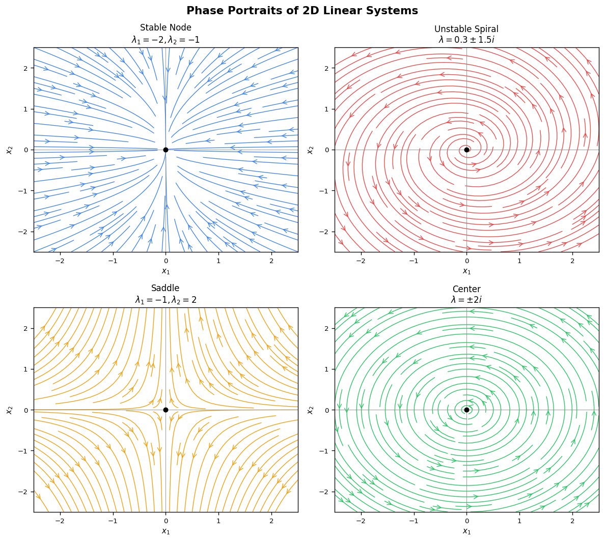
2.4 Classification of 2D Linear Systems

The long-term behavior of solutions to \( \dot{x} = Ax \) is determined by the eigenvalues of \( A \). For \( n = 2 \), let \( \lambda_1, \lambda_2 \) be the eigenvalues (real or complex conjugates). Define the trace \( \tau = \text{tr}(A) = \lambda_1 + \lambda_2 \) and determinant \( \Delta = \det(A) = \lambda_1 \lambda_2 \).

Real distinct eigenvalues (\( \Delta > 0 \), \( \tau^2 > 4\Delta \):

• Both negative (\( \lambda_1 < \lambda_2 < 0 \): stable node. All trajectories approach the origin tangent to the eigenvector of the less negative eigenvalue.
• Both positive (\( 0 < \lambda_1 < \lambda_2 \): unstable node. Time-reversed version.
• Opposite signs (\( \Delta < 0 \): saddle. The unstable manifold aligns with the eigenvector of the positive eigenvalue, the stable manifold with that of the negative eigenvalue.

Complex conjugate eigenvalues \( \lambda = \alpha \pm \beta i \) (\( \beta \neq 0 \):

• \( \alpha < 0 \): stable spiral. Trajectories spiral inward.
• \( \alpha > 0 \): unstable spiral. Trajectories spiral outward.
• \( \alpha = 0 \): centre. Trajectories are ellipses. Lyapunov stable but not asymptotically stable.

Repeated eigenvalues (\( \tau^2 = 4\Delta \):

• Diagonalizable (\( A = \lambda I \): star node. All lines through the origin are invariant.
• One Jordan block: improper node (degenerate node). Trajectories approach tangent to the single eigenvector direction.

The stability of the origin is summarized by the sign of the real parts: the origin is asymptotically stable if and only if all eigenvalues have strictly negative real part, i.e., \( \tau < 0 \) and \( \Delta > 0 \).

2.5 Contractions and Expansions

Liu’s notes emphasize the geometric interpretation of linear flows in terms of volume and distance.

Definition 2.3. The linear system \( \dot{x} = Ax \) is called a contraction if all eigenvalues of \( A \) have negative real parts, and an expansion if all eigenvalues have positive real parts.

For a contraction, the flow \( e^{At} \) shrinks distances: there exist constants \( C > 0 \) and \( \alpha > 0 \) such that

\[ \|e^{At} x\| \leq C e^{-\alpha t} \|x\| \quad \text{for all } t \geq 0. \]

This exponential decay rate is related to the spectral abscissa \( \mu(A) = \max_i \text{Re}(\lambda_i) \). Any \( \alpha < |\mu(A)| \) works as the decay rate, with the constant \( C \) absorbing the transient polynomial factors from Jordan blocks.

The Liouville formula connects the determinant of the flow to the trace of \( A \):

\[ \det(e^{At}) = e^{\text{tr}(A) \cdot t}. \]

Since \( \text{tr}(A) = \sum_i \lambda_i \), the flow expands volumes if \( \text{tr}(A) > 0 \), preserves them if \( \text{tr}(A) = 0 \), and contracts them if \( \text{tr}(A) < 0 \).

2.6 Nonhomogeneous Systems: Variation of Parameters

For the nonhomogeneous system \( \dot{x} = Ax + g(t) \), the solution with \( x(0) = x_0 \) is given by the variation of parameters formula:

\[ x(t) = e^{At} x_0 + \int_0^t e^{A(t-s)} g(s) \, ds. \]

This formula follows from multiplying both sides of the equation by the integrating factor \( e^{-At} \) and integrating. It shows that the response is a superposition of the free motion \( e^{At} x_0 \) and the convolution of the impulse response \( e^{At} \) with the forcing \( g(t) \).

2.7 Stability of Linear Systems

The long-term behavior of \( \dot{x} = Ax \) is completely characterized by the eigenvalues of \( A \):

• The equilibrium \( x^* = 0 \) is asymptotically stable if and only if all eigenvalues of \( A \) have strictly negative real parts.
• It is Lyapunov stable (but not asymptotically stable) if all eigenvalues have non-positive real parts and all purely imaginary eigenvalues correspond to diagonalizable blocks.
• It is unstable if any eigenvalue has positive real part, or if there is a purely imaginary eigenvalue with a non-trivial Jordan block.

Definition 2.4 (Stable, Unstable, Centre Subspaces). Decompose \( \mathbb{R}^n \) according to the eigenvalues of \( A \):

\[ E^s = \bigoplus_{\text{Re}(\lambda) < 0} V_\lambda, \quad E^u = \bigoplus_{\text{Re}(\lambda) > 0} V_\lambda, \quad E^c = \bigoplus_{\text{Re}(\lambda) = 0} V_\lambda. \]

These are \( A \)-invariant subspaces satisfying \( E^s \oplus E^u \oplus E^c = \mathbb{R}^n \). Trajectories starting in \( E^s \) decay to zero exponentially; those in \( E^u \) grow; those in \( E^c \) neither grow nor decay (they oscillate, or remain constant).

2.8 Coupled Oscillators and Normal Modes

The linear systems framework extends naturally to mechanical systems with multiple interacting bodies. Consider \( n \) masses coupled by springs. Each mass obeys Newton’s second law, but the forces depend on the positions of neighboring masses, coupling the equations of motion.

Equations of Motion. For two masses \( m_1, m_2 \) connected by three springs (spring constants \( k_1, k_2, k_3 \) between two walls, application of Hooke’s law and Newton’s second law gives

\[ \begin{pmatrix} m_1 & 0 \\ 0 & m_2 \end{pmatrix} \begin{pmatrix} \ddot{y}_1 \\ \ddot{y}_2 \end{pmatrix} + \begin{pmatrix} k_1 + k_2 & -k_2 \\ -k_2 & k_2 + k_3 \end{pmatrix} \begin{pmatrix} y_1 \\ y_2 \end{pmatrix} = \underline{c}, \]

which in operator notation is \( \hat{O}[y] = \underline{c} \) with \( \hat{O} \equiv MD^2 + K \). Here \( M \) is the mass matrix (diagonal, positive definite), \( K \) is the stiffness matrix (symmetric, positive semi-definite), and \( \underline{c} \) is a constant vector encoding the natural lengths of the springs.

Reduction to Homogeneous Form. By linearity, the general solution is the particular (equilibrium) solution plus the homogeneous solution. Setting \( y_i = \eta_i + x_i \) where \( K\underline{\eta} = \underline{c} \) defines the equilibrium positions \( \eta_i \), the displacements \( x_i(t) \) from equilibrium satisfy

\[ M\ddot{x} + Kx = 0. \]

For equal unit masses \( M = I \), this simplifies to \( \ddot{x} + Gx = 0 \) with \( G = K \). (When \( M \neq I \), one rescales coordinates to reduce to this form.)

Normal Mode Analysis. Substituting the trial solution \( x(t) = \underline{p}\cos(\omega t - \phi) \) into \( \ddot{x} + Gx = 0 \) gives

\[ \left[G - \omega^2 I\right]\underline{p} = 0. \]

This is an eigenvalue problem: \( \underline{p} \) must be an eigenvector of \( G \) with eigenvalue \( \lambda = \omega^2 \). Non-trivial solutions exist only when \( \det(G - \lambda I) = 0 \). Since \( G \) is real symmetric, all eigenvalues are real and eigenvectors are orthogonal.

Symmetric Example. Take \( m_1 = m_2 = 1 \) and \( k_1 = k_3 \) (left-right symmetric system). Then

\[ G = \begin{pmatrix} k_1 + k_2 & -k_2 \\ -k_2 & k_1 + k_2 \end{pmatrix}. \]

The characteristic equation \( (k_1 + k_2 - \lambda)^2 - k_2^2 = 0 \) gives two eigenvalues:

\[ \lambda_1 = k_1, \qquad \lambda_2 = k_1 + 2k_2, \]

with corresponding normalized eigenvectors (normal modes):

\[ \underline{p}^{(1)} = \frac{1}{\sqrt{2}}\begin{pmatrix}1\\1\end{pmatrix}, \qquad \underline{p}^{(2)} = \frac{1}{\sqrt{2}}\begin{pmatrix}1\\-1\end{pmatrix}. \]

Physical Interpretation.

• Mode 1 (frequency \( \omega_1 = \sqrt{k_1} \): the two masses oscillate in phase — \( x_1(t) = x_2(t) \). The central spring neither stretches nor compresses, so only the wall springs \( k_1 = k_3 \) determine the frequency.
• Mode 2 (frequency \( \omega_2 = \sqrt{k_1 + 2k_2} \): the two masses oscillate in antiphase — \( x_1(t) = -x_2(t) \). The central spring stretches twice as much as the wall springs, and both \( k_1 \) and \( k_2 \) contribute to the frequency.

General Solution. The general solution is a superposition of the two normal modes:

\[ x(t) = \beta^{(1)} \underline{p}^{(1)} \cos\left(\omega_1 t - \phi^{(1)}\right) + \beta^{(2)} \underline{p}^{(2)} \cos\left(\omega_2 t - \phi^{(2)}\right), \]

where the four constants \( \beta^{(1)}, \beta^{(2)}, \phi^{(1)}, \phi^{(2)} \) are determined by the four initial conditions \( x_1(0), x_2(0), \dot{x}_1(0), \dot{x}_2(0) \). Any motion of the system, however complex, decomposes uniquely into these two fundamental oscillations.

Connection to Linear Systems Theory. The normal mode analysis connects directly to the eigenstructure of the matrix \( A \) in the first-order reformulation. Writing \( z = (x, \dot{x})^T \), the system \( \ddot{x} + Gx = 0 \) becomes \( \dot{z} = Az \) with

\[ A = \begin{pmatrix} 0 & I \\ -G & 0 \end{pmatrix}. \]

The eigenvalues of \( A \) are \( \pm i\omega_j \) — purely imaginary, confirming that the undamped oscillator is a centre (Lyapunov stable but not asymptotically stable). The normal mode eigenvectors of \( G \) encode the spatial patterns of oscillation, while the eigenvalues \( \omega_j^2 \) give the squared frequencies.

---

Chapter 3: Nonlinear Local Theory

3.1 Linearization

The fundamental idea of local analysis is to approximate a nonlinear system near an equilibrium by its linearization.

Definition 3.1. Let \( x^* \) be an equilibrium of \( \dot{x} = f(x) \). Writing \( x = x^* + u \) and expanding,

\[ \dot{u} = f(x^* + u) = f(x^*) + Df(x^*) u + O(\|u\|^2) = Df(x^*) u + O(\|u\|^2), \]

since \( f(x^*) = 0 \). The linearization at \( x^* \) is the linear system \( \dot{u} = Df(x^*) u \) where \( Df(x^*) \) is the Jacobian matrix evaluated at the equilibrium.

Definition 3.2 (Hyperbolic Equilibrium). An equilibrium \( x^* \) is hyperbolic if no eigenvalue of \( Df(x^*) \) has zero real part — that is, \( E^c = \{0\} \).

3.2 The Hartman–Grobman Theorem

The Hartman–Grobman theorem is one of the cornerstones of dynamical systems theory. It states that, near a hyperbolic equilibrium, the nonlinear flow is topologically equivalent to the linearized flow.

Theorem 3.3 (Hartman–Grobman). Let \( x^* \) be a hyperbolic equilibrium of \( \dot{x} = f(x) \) with \( f \in C^1 \). Then there exists a neighborhood \( U \) of \( x^* \) and a homeomorphism \( h: U \to V \) (a continuous bijection with continuous inverse) mapping orbits of \( \dot{x} = f(x) \) to orbits of the linearization \( \dot{u} = Df(x^*) u \), preserving the direction of time.

The theorem says that near a hyperbolic equilibrium, the qualitative phase portrait of the nonlinear system is the same as that of its linearization — the two are related by a continuous (but generally not differentiable) change of coordinates. In particular:

• A hyperbolic stable equilibrium (all eigenvalues with negative real parts) of the linearization remains a stable equilibrium of the nonlinear system.
• A hyperbolic unstable equilibrium or saddle retains its character.
• If the equilibrium is non-hyperbolic (has purely imaginary eigenvalues), the Hartman–Grobman theorem does not apply, and the nonlinear terms can change the qualitative behavior (e.g., a center for the linearization might be a spiral for the nonlinear system).

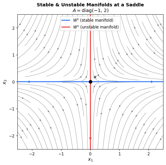
3.3 Stable and Unstable Manifold Theorem

For hyperbolic equilibria, the linear stable and unstable subspaces generalize to curved manifolds in the nonlinear setting.

Theorem 3.4 (Stable Manifold Theorem). Let \( x^* \) be a hyperbolic equilibrium of \( \dot{x} = f(x) \), with linearization having stable subspace \( E^s \) and unstable subspace \( E^u \). Then there exist locally invariant manifolds \( W^s_{\text{loc}}(x^*) \) and \( W^u_{\text{loc}}(x^*) \) (the local stable and unstable manifolds) such that:

1. \( W^s_{\text{loc}}(x^*) \) is tangent to \( E^s \) at \( x^* \), and every trajectory starting in \( W^s_{\text{loc}}(x^*) \) satisfies \( x(t) \to x^* \) as \( t \to +\infty \).
2. \( W^u_{\text{loc}}(x^*) \) is tangent to \( E^u \) at \( x^* \), and every trajectory starting in \( W^u_{\text{loc}}(x^*) \) satisfies \( x(t) \to x^* \) as \( t \to -\infty \).
3. Both manifolds are \( C^r \) if \( f \in C^r \).

The global stable manifold \( W^s(x^*) \) is obtained by flowing the local manifold backwards in time. Similarly, the global unstable manifold \( W^u(x^*) \) flows the local manifold forward. These objects organize the global phase portrait; the stable and unstable manifolds of saddle points in particular act as separatrices dividing the phase plane into qualitatively different regions.

3.4 Centre Manifold Theory

When the equilibrium is non-hyperbolic — when \( Df(x^*) \) has eigenvalues with zero real parts in addition to the stable/unstable ones — we cannot immediately apply Hartman–Grobman. The dynamics on the centre subspace \( E^c \) are not determined by the linear terms alone; nonlinear terms are crucial. The Centre Manifold Theorem allows us to reduce the study of the full system to a lower-dimensional system on the centre manifold.

Theorem 3.5 (Centre Manifold Theorem). Let the origin be an equilibrium of \( \dot{x} = f(x) \) with \( f \in C^r \), \( r \geq 2 \), and write the system in block form using the decomposition \( \mathbb{R}^n = E^c \oplus E^s \oplus E^u \):

\[ \dot{u} = Cu + F(u, v, w), \quad \dot{v} = Sv + G(u, v, w), \quad \dot{w} = Uw + H(u, v, w), \]

where \( C \) has eigenvalues with zero real part, \( S \) has eigenvalues with negative real part, and \( U \) has eigenvalues with positive real part. Then there exists a \( C^r \) centre manifold \( W^c \) of the form

\[ W^c = \{(u, v, w) : v = h_1(u), \ w = h_2(u), \ h_i(0) = 0, \ Dh_i(0) = 0\} \]

for smooth functions \( h_i \) defined in a neighborhood of the origin. The centre manifold is locally invariant and tangent to \( E^c \) at the origin.

The reduced system on the centre manifold is \( \dot{u} = Cu + F(u, h_1(u), h_2(u)) \), which is a system on \( \dim E^c \) dimensions. If the origin is stable for this reduced system, it is stable for the full system; if unstable on the centre manifold, it is unstable in the full system.

Finding the Centre Manifold. The functions \( h_i \) satisfy a quasilinear PDE called the centre manifold equation, obtained by differentiating \( v = h_1(u) \):

\[ Dh_1(u)(Cu + F(u,h_1(u), h_2(u))) = Sh_1(u) + G(u, h_1(u), h_2(u)). \]

This is typically solved approximately by expanding in power series, matching terms order by order. At leading order, \( h_i(u) = O(\|u\|^2) \), and higher-order terms can be computed iteratively.

3.5 Lyapunov Functions

Lyapunov’s direct method provides stability information without requiring an explicit formula for solutions.

Definition 3.6. A function \( V: U \to \mathbb{R} \) defined on a neighborhood \( U \) of the origin is called a Lyapunov function for \( \dot{x} = f(x) \) if:

1. \( V(0) = 0 \) and \( V(x) > 0 \) for \( x \neq 0 \) in \( U \) (positive definite).
2. The orbital derivative \( \dot{V}(x) = \nabla V(x) \cdot f(x) \leq 0 \) in \( U \) (non-increasing along trajectories).

Theorem 3.7 (Lyapunov Stability Theorem). If a Lyapunov function \( V \) exists with \( \dot{V}(x) \leq 0 \), the origin is Lyapunov stable. If additionally \( \dot{V}(x) < 0 \) for \( x \neq 0 \) (strictly negative definite), the origin is asymptotically stable.

The intuition is elegant: \( V \) measures a generalized “energy” or “distance from the origin.” If the energy is always non-increasing along orbits, the system cannot escape from level sets of \( V \), ensuring stability.

Example. For the nonlinear system \( \dot{x}_1 = -x_1 + x_2^2 \), \( \dot{x}_2 = -x_2 \), take \( V(x) = x_1^2 + x_2^2 \). Then

\[ \dot{V} = 2x_1(-x_1 + x_2^2) + 2x_2(-x_2) = -2x_1^2 + 2x_1 x_2^2 - 2x_2^2. \]

Near the origin, the term \( 2x_1 x_2^2 \) is dominated by \( -2x_1^2 - 2x_2^2 \), so \( \dot{V} < 0 \) in a sufficiently small neighborhood, confirming asymptotic stability.

3.6 La Salle’s Invariance Principle

Lyapunov’s direct method requires \( \dot{V} < 0 \) for asymptotic stability. La Salle’s principle weakens this requirement by using the geometric properties of the flow.

Theorem 3.8 (La Salle’s Invariance Principle). Let \( V: \mathbb{R}^n \to \mathbb{R} \) be a \( C^1 \) function with \( \dot{V}(x) \leq 0 \) along trajectories of \( \dot{x} = f(x) \). Let \( \Omega_c = \{x: V(x) \leq c\} \) be a compact positively invariant set. Define \( E = \{x \in \Omega_c : \dot{V}(x) = 0\} \) and let \( M \) be the largest invariant set contained in \( E \). Then every solution starting in \( \Omega_c \) converges to \( M \) as \( t \to \infty \).

La Salle’s principle is particularly useful when \( \dot{V} = 0 \) on a set larger than just the equilibrium. For instance, in the mass-spring system with linear damping, \( \dot{V} = 0 \) only when the velocity is zero; but checking that the only invariant set in \( E \) is the origin confirms asymptotic stability even when \( \dot{V} \) is not strictly negative definite everywhere.

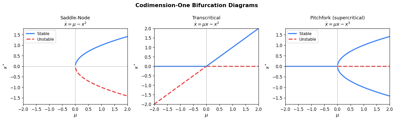
3.7 Introduction to Bifurcations

A bifurcation occurs when a qualitative change in the phase portrait takes place as a parameter passes through a critical value. We introduce here the three primary codimension-one bifurcations for equilibria.

Consider a one-parameter family \( \dot{x} = f(x, \mu) \) where \( \mu \in \mathbb{R} \) is a parameter, and suppose the origin is an equilibrium with one zero eigenvalue of \( D_x f(0, 0) \).

Saddle-Node Bifurcation. This is the generic way in which two equilibria (one stable, one unstable) collide and annihilate, or are created. The normal form on the centre manifold is

\[ \dot{x} = \mu - x^2. \]

For \( \mu < 0 \), no equilibria exist; at \( \mu = 0 \), a semi-stable equilibrium appears at the origin; for \( \mu > 0 \), two equilibria exist at \( x = \pm\sqrt{\mu} \) (one stable, one unstable).

Transcritical Bifurcation. Two equilibria exist for all parameter values near \( \mu = 0 \) but exchange stability as \( \mu \) passes through zero. The normal form is

\[ \dot{x} = \mu x - x^2 = x(\mu - x). \]

For any \( \mu \), there are equilibria at \( x = 0 \) and \( x = \mu \). When \( \mu < 0 \), \( x = 0 \) is stable and \( x = \mu \) is unstable; when \( \mu > 0 \), the stabilities exchange.

Pitchfork Bifurcation. A symmetric bifurcation where one equilibrium splits into three. The normal form (supercritical) is

\[ \dot{x} = \mu x - x^3. \]

For \( \mu \leq 0 \), only \( x = 0 \) is an equilibrium (stable). For \( \mu > 0 \), the origin becomes unstable and two new stable equilibria appear at \( x = \pm\sqrt{\mu} \). The subcritical pitchfork has the form \( \dot{x} = \mu x + x^3 \), where for \( \mu < 0 \) the origin is stable with two flanking unstable equilibria at \( x = \pm\sqrt{-\mu} \), and for \( \mu > 0 \) only the unstable origin remains.

---

Chapter 4: Nonlinear Global Theory and Periodic Solutions

4.1 Periodic Solutions

While local theory studies behavior near equilibria, global theory concerns the long-time behavior for general initial conditions. A particularly important class of behavior consists of periodic solutions.

Definition 4.1. A solution \( x(t) \) is periodic with period \( T > 0 \) if \( x(t + T) = x(t) \) for all \( t \). The smallest such \( T \) is the minimal period. The orbit of a periodic solution is a closed curve in phase space called a closed orbit or cycle.

Periodic solutions are especially important in two-dimensional systems, where they are the only type of recurrent behavior besides equilibria (by the Poincaré–Bendixson theorem, treated below).

4.2 Floquet Theory

When a periodic solution exists, one can study the stability of nearby solutions using Floquet theory. Consider a system with a known periodic solution \( \gamma(t) \) of period \( T \). Write \( x(t) = \gamma(t) + u(t) \) and linearize to obtain the variational equation:

\[ \dot{u} = Df(\gamma(t)) u, \]

a linear system with \( T \)-periodic coefficients.

Theorem 4.2 (Floquet). Let \( \Phi(t) \) be the fundamental matrix solution of \( \dot{u} = A(t) u \) with \( \Phi(0) = I \), where \( A(t) \) is \( T \)-periodic. Then

\[ \Phi(t + T) = \Phi(t) M, \]

where \( M = \Phi(T) \) is the monodromy matrix. There exists a (possibly complex) matrix \( B \) with \( e^{BT} = M \) and a \( T \)-periodic matrix function \( P(t) \) such that

\[ \Phi(t) = P(t) e^{Bt}. \]

The eigenvalues of the monodromy matrix \( M \) are called Floquet multipliers (or characteristic multipliers). Their logarithms divided by \( T \) are the Floquet exponents (or characteristic exponents).

Stability via Floquet multipliers. A periodic solution is asymptotically stable (orbitally) if all Floquet multipliers except one lie strictly inside the unit circle \( |\mu| < 1 \). (One multiplier is always exactly 1, corresponding to perturbations along the periodic orbit itself.) It is unstable if any multiplier has \( |\mu| > 1 \).

Proposition 4.3 (Product Formula for Floquet Multipliers). For the \( n \times n \) variational equation, the product of all Floquet multipliers is

\[ \prod_{i=1}^n \mu_i = \det(\Phi(T)) = \exp\left(\int_0^T \text{tr}(Df(\gamma(t))) \, dt\right). \]

This follows from Liouville’s formula. For a 2D system \( \dot{x} = f(x) \), one multiplier is always \( \mu_1 = 1 \), so the other is

\[ \mu_2 = \exp\left(\int_0^T \text{tr}(Df(\gamma(t))) \, dt\right) = \exp\left(\int_0^T (\partial_{x_1} f_1 + \partial_{x_2} f_2) \, dt\right). \]

The sign of this exponent determines the orbital stability: \( |\mu_2| < 1 \) (stable) if and only if \( \int_0^T \text{div}(f) \, dt < 0 \).

4.3 Poincaré Maps and Limit Cycles

An important tool for studying periodic solutions is the Poincaré map (or first return map). Given a periodic orbit \( \Gamma \), choose a codimension-one section \( \Sigma \) transverse to \( \Gamma \). For points \( x \in \Sigma \) near \( \Gamma \cap \Sigma \), the forward orbit returns to \( \Sigma \) at a point \( P(x) \). The map \( P: \Sigma \to \Sigma \) is the Poincaré map.

Fixed points of \( P \) correspond to periodic orbits of the flow. The stability of the periodic orbit is determined by the eigenvalues of \( DP(x^*) \) at the fixed point — these are precisely the non-trivial Floquet multipliers.

Definition 4.4 (Limit Cycle). An isolated closed orbit — a periodic orbit that has no other closed orbits in a neighborhood — is called a limit cycle. A limit cycle is stable (or attracting) if nearby trajectories spiral toward it as \( t \to +\infty \), unstable (or repelling) if they spiral away, and semi-stable if attracted from one side and repelled from the other.

Limit cycles are a purely nonlinear phenomenon; linear systems cannot have isolated closed orbits (in a linear center, every closed orbit is part of a family parameterized by initial conditions, not isolated).

4.4 The Poincaré–Bendixson Theorem

In the plane, the possible long-term behaviors of trajectories are highly restricted.

Theorem 4.5 (Poincaré–Bendixson). Let \( \dot{x} = f(x) \) be a \( C^1 \) system in \( \mathbb{R}^2 \). If a trajectory \( x(t) \) remains in a compact region \( D \) for all \( t \geq 0 \), and \( D \) contains only finitely many equilibria, then the \( \omega \)-limit set \( \omega(x) \) is one of:

1. An equilibrium point,
2. A periodic orbit,
3. A homoclinic or heteroclinic cycle — a collection of equilibria connected by orbits.

Here the \( \omega \)-limit set of a trajectory is \( \omega(x) = \{y : \exists t_n \to \infty, \phi_{t_n}(x) \to y\} \).

Proof sketch. The key insight uses the Jordan curve theorem: any closed curve in \( \mathbb{R}^2 \) divides the plane into an interior and exterior. If the \( \omega \)-limit set contains a point that is not an equilibrium, any trajectory in the \( \omega \)-limit set that starts at such a point must have its own \( \omega \)-limit set again within \( D \). Using the non-crossing property of orbits and the topology of the plane, one shows the only possibilities are closed orbits or connections between equilibria.

The Poincaré–Bendixson theorem is a powerful tool for proving the existence of periodic orbits: if one can construct an annular trapping region — a compact set bounded by two curves such that the vector field points inward on both boundaries — and this region contains no equilibria, then it must contain a periodic orbit.

4.5 Dulac’s Criterion

Dulac’s criterion provides a sufficient condition for the absence of closed orbits.

Theorem 4.6 (Dulac’s Criterion). Let \( \dot{x} = f(x) \) be a \( C^1 \) system on a simply connected region \( D \subseteq \mathbb{R}^2 \). If there exists a \( C^1 \) function \( B(x) \) (a Dulac function) such that

\[ \text{div}(B f) = \frac{\partial (B f_1)}{\partial x_1} + \frac{\partial (B f_2)}{\partial x_2} \]

is of one sign (does not change sign and is not identically zero) in \( D \), then \( \dot{x} = f(x) \) has no closed orbits in \( D \).

Proof. Suppose for contradiction that \( \Gamma \) is a closed orbit in \( D \), enclosing a region \( R \). By Green’s theorem (divergence theorem in 2D),

\[ \iint_R \text{div}(Bf) \, dA = \oint_{\Gamma} B f \cdot n \, ds. \]

But since \( \Gamma \) is an orbit of \( f \), the vector \( f \) is tangent to \( \Gamma \), so \( f \cdot n = 0 \) on \( \Gamma \). Thus the right side is zero. But the left side is nonzero since \( \text{div}(Bf) \) has one sign. Contradiction.

Special case: Bendixson’s criterion. Taking \( B \equiv 1 \), we get: if \( \text{div}(f) = \partial f_1/\partial x_1 + \partial f_2/\partial x_2 \) has one sign on a simply connected region \( D \), there are no closed orbits in \( D \).

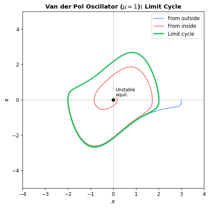
4.6 Liénard Systems and the Van der Pol Equation

A broad class of oscillator models fits the Liénard equation:

\[ \ddot{x} + f(x) \dot{x} + g(x) = 0, \]

or equivalently in system form with \( y = \dot{x} \):

\[ \dot{x} = y, \qquad \dot{y} = -f(x)y - g(x). \]

The Van der Pol equation is the canonical example, with \( f(x) = \mu(x^2 - 1) \) and \( g(x) = x \):

\[ \ddot{x} + \mu(x^2 - 1)\dot{x} + x = 0. \]

For \( \mu > 0 \), the damping is negative for \( |x| < 1 \) (energy input) and positive for \( |x| > 1 \) (energy dissipation). This self-sustaining oscillation is responsible for the existence and uniqueness of a stable limit cycle for any \( \mu > 0 \).

Theorem 4.7 (Liénard, Uniqueness of Limit Cycle). For the Van der Pol equation with \( \mu > 0 \), there exists a unique stable limit cycle, and all non-equilibrium orbits tend to this cycle as \( t \to \infty \).

More generally, for a Liénard system, suppose:

1. \( g \) is odd: \( g(-x) = -g(x) \), and \( g(x) > 0 \) for \( x > 0 \).
2. \( f \) is even: \( f(-x) = f(x) \).
3. \( F(x) = \int_0^x f(s) \, ds \) has exactly one positive zero at \( x = a \), is negative for \( 0 < x < a \), and tends to \( +\infty \) for \( x \to \infty \).

Theorem 4.8 (Liénard’s Theorem). Under the above conditions, the Liénard system has exactly one limit cycle, and it is stable.

4.7 Hamiltonian Systems

Definition 4.9. A Hamiltonian system on \( \mathbb{R}^{2n} \) with coordinates \( (q, p) \in \mathbb{R}^n \times \mathbb{R}^n \) is defined by a smooth function \( H(q, p) \) (the Hamiltonian or total energy) via

\[ \dot{q}_i = \frac{\partial H}{\partial p_i}, \qquad \dot{p}_i = -\frac{\partial H}{\partial q_i}, \quad i = 1, \ldots, n. \]

The Hamiltonian is a first integral (conserved quantity): \( \dot{H} = \sum_i (\partial H/\partial q_i) \dot{q}_i + (\partial H/\partial p_i) \dot{p}_i = 0 \) along any solution. Thus every trajectory lies on a level set \( H = \text{const} \).

Proposition 4.10 (No Asymptotically Stable Equilibria). A Hamiltonian system has no asymptotically stable equilibria. More strongly, it is volume-preserving: the divergence of the vector field is

\[ \text{div}(f) = \sum_i \left(\frac{\partial^2 H}{\partial q_i \partial p_i} - \frac{\partial^2 H}{\partial p_i \partial q_i}\right) = 0. \]

By Liouville’s theorem, the flow \( \phi_t \) preserves phase-space volume. This rules out attracting limit cycles and attracting equilibria alike.

Corollary 4.11 (No Limit Cycles). A Hamiltonian system in \( \mathbb{R}^2 \) has no limit cycles. Any closed orbit is a member of a continuous family parameterized by the energy level.

Proposition 4.12 (Centers near Stable Equilibria). In a 2D Hamiltonian system, if \( (q^*, p^*) \) is an equilibrium and the Hessian of \( H \) at \( (q^*, p^*) \) is positive definite (a local energy minimum), then the equilibrium is a center — it is surrounded by closed orbits.

4.8 Gradient Systems

Definition 4.13. A system \( \dot{x} = f(x) \) is a gradient system if there exists a smooth function \( V: \mathbb{R}^n \to \mathbb{R} \) such that \( f(x) = -\nabla V(x) \).

Gradient systems are in many ways opposite to Hamiltonian systems: they dissipate energy and have no closed orbits.

Proposition 4.14. A gradient system has no closed orbits.

Proof. Suppose \( x(t) \) is a periodic solution with period \( T \). Then

\[ 0 = V(x(T)) - V(x(0)) = \int_0^T \frac{d}{dt} V(x(t)) \, dt = \int_0^T \nabla V(x) \cdot \dot{x} \, dt = -\int_0^T \|\nabla V(x)\|^2 \, dt. \]

This forces \( \nabla V = 0 \) along the entire orbit, so every point on the orbit is an equilibrium. But a periodic orbit consists of non-equilibrium points, contradiction.

Proposition 4.15. Every \( \omega \)-limit set of a gradient system consists entirely of equilibria. Generically (when all equilibria are isolated), every bounded trajectory converges to an equilibrium.

This is because \( \dot{V} = -\|\nabla V\|^2 \leq 0 \), so \( V \) decreases along orbits. The \( \omega \)-limit set lies on the set where \( \dot{V} = 0 \), i.e., where \( \nabla V = 0 \) — precisely the equilibria.

4.9 Homoclinic and Heteroclinic Orbits

Definition 4.16. A homoclinic orbit is an orbit whose \( \alpha \)-limit set and \( \omega \)-limit set are both the same equilibrium — it connects an equilibrium to itself. A heteroclinic orbit connects two distinct equilibria, with one as the \( \alpha \)-limit and the other as the \( \omega \)-limit.

A homoclinic cycle (or saddle connection) consists of a homoclinic orbit together with its equilibrium. In the plane, such connections form the third possibility in the Poincaré–Bendixson theorem. They can appear at bifurcation points, and their presence or destruction plays a role in creating or destroying limit cycles.

4.10 Structural Stability

A dynamical system is structurally stable if its qualitative behavior is preserved under small perturbations of the vector field. More precisely:

Definition 4.17. A \( C^1 \) vector field \( f \) on a compact region \( D \) is structurally stable if for every \( \epsilon > 0 \), there exists \( \delta > 0 \) such that any vector field \( g \) with \( \|f - g\|_{C^1} < \delta \) is topologically equivalent to \( f \) on \( D \).

Theorem 4.18 (Peixoto, 1962). A \( C^1 \) vector field on a compact 2-manifold is structurally stable if and only if:

1. All equilibria are hyperbolic.
2. All periodic orbits are hyperbolic (non-unit Floquet multipliers other than the trivial one).
3. There are no homoclinic or heteroclinic connections.

Structurally unstable systems — those with non-hyperbolic equilibria, non-hyperbolic periodic orbits, or saddle connections — are the “bifurcation points” in the space of all vector fields. They represent the codimension-one boundaries between structurally stable regions in function space.

4.11 Bifurcation Theory

We return to bifurcations, now in the global context. A bifurcation of a parametrized family \( \dot{x} = f_\mu(x) \) occurs at a parameter value \( \mu_0 \) where the system is not structurally stable. We have already encountered codimension-one equilibrium bifurcations (saddle-node, transcritical, pitchfork). We now discuss bifurcations involving periodic orbits.

Saddle-Node Bifurcation of Periodic Orbits. Two periodic orbits (one stable, one unstable) collide and disappear, analogous to the equilibrium case. The Poincaré map’s fixed point undergoes a fold bifurcation.

Period-Doubling Bifurcation. A Floquet multiplier passes through \( -1 \). The original periodic orbit loses stability, and a new orbit of twice the period is born.

Torus Bifurcation (Neimark–Sacker). Two complex conjugate Floquet multipliers cross the unit circle. A periodic orbit loses stability and is replaced by an invariant torus (quasi-periodic or periodic motion on the torus).

4.12 Hopf Bifurcation

The Hopf bifurcation is the most important mechanism by which equilibria give birth to periodic orbits. It occurs when, as a parameter \( \mu \) varies, a pair of complex conjugate eigenvalues of the linearization crosses the imaginary axis.

Setup. Consider \( \dot{x} = f(x, \mu) \) in \( \mathbb{R}^2 \) (or in the plane of the centre manifold for higher-dimensional systems). Suppose the origin is an equilibrium for all \( \mu \), and the linearization \( A(\mu) = D_x f(0, \mu) \) has complex conjugate eigenvalues

\[ \lambda(\mu) = \alpha(\mu) \pm i \beta(\mu) \]

with \( \alpha(0) = 0 \), \( \beta(0) = \beta_0 \neq 0 \), and the transversality condition \( \alpha'(0) = d\alpha/d\mu|_{\mu=0} \neq 0 \).

Example (polar coordinates). The canonical Hopf bifurcation is:

\[ \dot{r} = \mu r - r^3, \qquad \dot{\theta} = 1. \]

In Cartesian coordinates, this is \( \dot{x}_1 = \mu x_1 - x_2 - x_1(x_1^2 + x_2^2) \), \( \dot{x}_2 = x_1 + \mu x_2 - x_2(x_1^2 + x_2^2) \). The radial equation decouples: for \( \mu \leq 0 \), \( r = 0 \) is the only non-negative equilibrium of \( \dot{r} = r(\mu - r^2) \) and it is stable. For \( \mu > 0 \), a new equilibrium appears at \( r^* = \sqrt{\mu} \), corresponding to a periodic orbit of the original system with radius \( \sqrt{\mu} \) and frequency \( 1 \).

Theorem 4.19 (Poincaré–Andronov–Hopf). Under the above transversality condition, there exists a family of periodic orbits bifurcating from the origin at \( \mu = 0 \). Define the first Lyapunov coefficient \( \sigma \) via the Taylor expansion of \( f \) at the origin:

\[ \sigma = \frac{1}{16}\left[ f^1_{xxx} + f^1_{xyy} + f^2_{xxy} + f^2_{yyy} \right] + \frac{1}{16\beta_0}\left[ f^1_{xy}(f^1_{xx} + f^1_{yy}) - f^2_{xy}(f^2_{xx} + f^2_{yy}) - f^1_{xx}f^2_{xx} + f^1_{yy}f^2_{yy} \right], \]

where superscripts denote components and subscripts denote partial derivatives evaluated at the origin.

• Supercritical Hopf bifurcation (\( \sigma < 0 \): For \( \mu < 0 \), the origin is a stable spiral. At \( \mu = 0 \) it is a stable (weakly) nonlinear center. For \( \mu > 0 \), a stable limit cycle of radius \( O(\sqrt{\mu}) \) is born, and the origin becomes an unstable spiral.
• Subcritical Hopf bifurcation (\( \sigma > 0 \): For \( \mu < 0 \), an unstable limit cycle surrounds the stable equilibrium. At \( \mu = 0 \), the cycle collapses onto the origin. For \( \mu > 0 \), the origin is unstable with no limit cycle nearby — trajectories may escape to large amplitude.

The Hopf bifurcation is fundamentally important in applications: it is the generic mechanism by which oscillations arise spontaneously in physical, biological, and engineering systems as a parameter (such as a feedback gain or flow rate) is varied.

---

Appendix: Key Theorems Reference

The table below collects the principal results of the course.

Theorem	Statement	Context
Picard–Lindelöf	Local existence and uniqueness for locally Lipschitz \( f \)	Ch. 1
Hartman–Grobman	Nonlinear flow ≈ linearized flow near hyperbolic equilibria	Ch. 3
Stable Manifold	\( W^s, W^u \) are \( C^r \) manifolds tangent to \( E^s, E^u \)	Ch. 3
Centre Manifold	Reduce dynamics to the centre subspace	Ch. 3
Lyapunov	\( V > 0, \dot{V} \leq 0 \Rightarrow \) stable	Ch. 3
La Salle	Trajectories converge to largest invariant set where \( \dot{V} = 0 \)	Ch. 3
Floquet	Periodic linear systems via monodromy matrix	Ch. 4
Floquet (product)	\( \prod \mu_i = \exp\int_0^T \text{tr}(Df(\gamma)) \, dt \)	Ch. 4
Poincaré–Bendixson	\( \omega \)-limit sets in \( \mathbb{R}^2 \): equilibrium, periodic orbit, or connection	Ch. 4
Dulac’s Criterion	\( \text{div}(Bf) \) of one sign \( \Rightarrow \) no closed orbits	Ch. 4
Liénard	Conditions for unique stable limit cycle	Ch. 4
Hopf Bifurcation	Eigenvalues cross imaginary axis \( \Rightarrow \) limit cycle born	Ch. 4
No Cycles (Hamiltonian)	Volume-preserving \( \Rightarrow \) no asymptotically stable sets	Ch. 4
No Cycles (Gradient)	\( f = -\nabla V \Rightarrow \) no closed orbits	Ch. 4
Peixoto	Characterization of structurally stable 2D flows	Ch. 4