Quantum mechanics is, without exaggeration, the most precisely tested physical theory ever constructed. Its predictions agree with experiment to better than one part in a billion in some domains, and yet its conceptual foundations remain genuinely strange: particles that exist as probability waves, quantities that cannot be simultaneously measured with arbitrary precision, and a measurement process that seems to disturb the very system being observed. This course develops the mathematical machinery of non-relativistic quantum mechanics from first principles, moving from the historical motivations through the formal axioms to applications ranging from atomic structure to perturbation theory.

The logical arc of the notes proceeds as follows. We first recall the Hamiltonian formulation of classical mechanics, which already contains the seeds of quantum theory in the algebraic structure of Poisson brackets. We then examine the experimental evidence that forced physicists in the early twentieth century to abandon classical wave theory in favour of a probabilistic description of matter waves. The bulk of the course is concerned with solving the Schrödinger equation — first for free particles, then for a variety of one-dimensional potentials, then in three dimensions leading to the hydrogen atom. We conclude with electron spin, the Zeeman effect, and the two principal approximation methods: perturbation theory and the variational principle.

Chapter 1: From Classical to Quantum

Section 1.1: The Classical Framework and the Quantum Revolution

1.1 Hamiltonian Mechanics

Classical mechanics admits two equivalent formulations: the Lagrangian, which describes dynamics via a variational principle, and the Hamiltonian, which reformulates everything in terms of generalized coordinates and their conjugate momenta. The Hamiltonian framework is the natural precursor to quantum mechanics, because the algebraic relations it introduces — Poisson brackets — survive the passage to the quantum theory as commutators.

For a particle of mass \(m\) moving in a potential \(U(x)\), the Hamiltonian is the total mechanical energy expressed as a function of position \(x\) and momentum \(p\):

\[H(x,p) = \frac{p^2}{2m} + U(x).\]

Hamilton’s equations of motion then determine how \(x\) and \(p\) evolve in time:

\[\dot{x} = \frac{\partial H}{\partial p} = \frac{p}{m}, \qquad \dot{p} = -\frac{\partial H}{\partial x} = -\frac{dU}{dx}.\]

The first equation identifies momentum as \(p = m\dot{x}\), and the second is Newton’s second law \(\dot{p} = F = -dU/dx\). The Hamiltonian framework thus reproduces Newtonian mechanics while simultaneously making the momentum \(p\) an independent dynamical variable on equal footing with the position \(x\).

The Poisson bracket of two phase-space functions \(f(x,p)\) and \(g(x,p)\) is defined as

\[\{f, g\} = \frac{\partial f}{\partial x}\frac{\partial g}{\partial p} - \frac{\partial f}{\partial p}\frac{\partial g}{\partial x}.\]

In this language, Hamilton’s equations take the compact form \(\dot{x} = \{x, H\}\) and \(\dot{p} = \{p, H\}\), and more generally any dynamical variable \(f\) satisfies \(\dot{f} = \{f, H\}\). The fundamental Poisson brackets of position and momentum are

\[\{x, p\} = 1, \qquad \{x, x\} = 0, \qquad \{p, p\} = 0.\]

A quantity is conserved if and only if its Poisson bracket with the Hamiltonian vanishes: \(\{f, H\} = 0\). In particular, the energy \(H\) itself satisfies \(\{H, H\} = 0\), so total energy is conserved whenever \(H\) does not depend explicitly on time.

When we pass to quantum mechanics, the Poisson bracket structure is replaced by commutators of operators. Dirac’s quantization rule — which we will make precise in Chapter 6 — replaces \(\{f, g\} \to \frac{1}{i\hbar}[\hat{f}, \hat{g}]\), so the classical relation \(\{x, p\} = 1\) becomes the canonical commutation relation \([\hat{x}, \hat{p}] = i\hbar\). This algebraic bridge between the classical and quantum worlds is not a derivation but a correspondence that has proven extraordinarily successful.

1.2 The Quantum Hypothesis: Photons and Matter Waves

By the end of the nineteenth century, classical physics appeared triumphant. Maxwell’s electromagnetic theory described light as a continuous wave propagating through the ether, and statistical mechanics gave a satisfying account of heat and thermodynamics. Two clouds on the horizon — the ultraviolet catastrophe in blackbody radiation and the photoelectric effect — would ultimately require an entirely new physics.

Light as a wave. Maxwell’s equations predict that electromagnetic waves in vacuum satisfy the wave equation

\[\frac{\partial^2 E}{\partial x^2} - \frac{1}{c^2}\frac{\partial^2 E}{\partial t^2} = 0,\]

with plane-wave solutions \(E \propto e^{i(kx - \omega t)}\) obeying the linear dispersion relation \(\omega = ck\). Here \(k = 2\pi/\lambda\) is the wave number, \(\omega = 2\pi f\) is the angular frequency, and \(c \approx 3\times 10^8\) m/s is the speed of light. Because the dispersion is linear, all frequencies travel at the same speed: a light pulse maintains its shape indefinitely in vacuum.

The photoelectric effect and photons. In 1887, Hertz discovered that ultraviolet light can eject electrons from a metal surface — the photoelectric effect. Classical wave theory predicts that increasing the light intensity should increase the kinetic energy of the ejected electrons, and that sufficiently intense low-frequency light should also eject electrons. Neither prediction is correct. Instead, experiment shows:

• There is a minimum frequency \(f_0\) (the threshold frequency) below which no electrons are emitted, regardless of intensity.
• Above the threshold, the kinetic energy of ejected electrons is \(K = hf - W\), where \(W\) is the work function of the metal and \(h\) is Planck’s constant.
• The intensity of light controls the number of ejected electrons, not their energy.

Einstein explained this in 1905 by proposing that light consists of discrete quanta — photons — each carrying energy \(E = hf = \hbar\omega\), where \(\hbar = h/(2\pi) \approx 1.055 \times 10^{-34}\) J·s is the reduced Planck constant. The photoelectric effect then becomes a collision between one photon and one electron: the photon gives up all its energy, some of which overcomes the work function and the rest appears as kinetic energy.

The photon also carries momentum. Since photons are massless and travel at speed \(c\), their energy and momentum are related by \(E = pc\), so \(p = E/c = \hbar\omega/c = \hbar k\). In terms of the de Broglie wavelength \(\lambda\), this reads \(p = h/\lambda\).

Matter waves and de Broglie. In 1924, de Broglie made a bold conjecture: if light — traditionally a wave — behaves like a particle, then perhaps matter — traditionally a particle — should also exhibit wave-like behaviour. He proposed that a particle of momentum \(p\) is associated with a wave of wavelength

\[\lambda = \frac{h}{p}, \quad \text{or equivalently} \quad p = \hbar k.\]

This hypothesis was confirmed experimentally by Davisson and Germer in 1927, who observed diffraction of electrons from a crystalline nickel surface. The diffraction pattern was exactly what one would predict for a wave with the de Broglie wavelength corresponding to the electron’s momentum.

Dispersion for matter waves. A free non-relativistic particle of mass \(m\) has kinetic energy \(E = p^2/(2m) = \hbar^2 k^2/(2m)\). Since \(E = \hbar\omega\), this gives the quadratic dispersion relation

\[\omega(k) = \frac{\hbar k^2}{2m}.\]

This is fundamentally different from the linear dispersion \(\omega = ck\) of light. As we will see in Chapter 2, the quadratic dispersion causes wave packets of matter to spread in time — a purely quantum-mechanical effect with no classical analogue.

1.3 Classical Wave Packets

Before diving into quantum mechanics, it is instructive to understand how wave packets behave in classical physics. A monochromatic plane wave \(e^{i(kx-\omega t)}\) is spatially delocalized — it extends to infinity in both directions and carries no information about the position of a particle. To describe a localized object, we form a wave packet by superposing plane waves with a range of wave numbers:

\[\Psi(x,t) = \frac{1}{\sqrt{2\pi}}\int_{-\infty}^{\infty} \Phi(k)\, e^{i(kx-\omega(k)t)}\, dk.\]

The function \(\Phi(k)\) is the Fourier transform of the initial profile \(\Psi(x,0)\) and determines how much each wave number contributes to the packet. A narrow packet in position space requires a broad spread of wave numbers (and vice versa), anticipating the Heisenberg uncertainty principle.

For electromagnetic waves with \(\omega = ck\), consider a wave packet peaked around wave number \(k_0\). Each frequency component travels at the same speed \(c\), so the entire packet moves rigidly at speed \(c\) without distortion. This undistorted propagation is a special property of linear dispersion and does not persist for matter waves, where \(\omega \propto k^2\).

Chapter 2: The Schrödinger Wave Mechanics

Section 2.1: Wave Packets and Probabilistic Interpretation

2.1 Born’s Rule and the Momentum Representation

Given the de Broglie hypothesis, how do we interpret the wave function \(\Psi(x,t)\) that describes a quantum particle? The answer — provided by Max Born in 1926 — is that \(\Psi\) is a probability amplitude: the probability of finding the particle in the interval \([x, x+dx]\) at time \(t\) is

\[dP = |\Psi(x,t)|^2\, dx.\]

The quantity \(\rho(x,t) = |\Psi(x,t)|^2\) is the probability density. For this interpretation to be consistent, the wave function must be normalizable:

\[\int_{-\infty}^{\infty} |\Psi(x,t)|^2\, dx = 1.\]

A wave function is written as a superposition of momentum eigenstates (plane waves) via the Fourier transform:

\[\Psi(x,t) = \frac{1}{\sqrt{2\pi\hbar}}\int_{-\infty}^{\infty} \tilde{\phi}(p,t)\, e^{ipx/\hbar}\, dp,\]

where \(\tilde{\phi}(p,t)\) is the momentum-space wave function. By Parseval’s theorem (proved below), the normalization in position space equals the normalization in momentum space:

\[\int_{-\infty}^{\infty} |\Psi(x,t)|^2\, dx = \int_{-\infty}^{\infty} |\tilde{\phi}(p,t)|^2\, \frac{dp}{\hbar} = 1.\]

So \(D(p) = |\tilde{\phi}(p,t)|^2/\hbar\) plays the role of a probability density for momentum, and the probability of measuring momentum in \([p, p+dp]\) is \(D(p)\,dp = |\tilde{\phi}(p,t)|^2\, dp/\hbar\).

In terms of wave number \(k = p/\hbar\), we write

\[\Psi(x,t) = \frac{1}{\sqrt{2\pi}}\int_{-\infty}^{\infty} \Phi(k,t)\, e^{ikx}\, dk, \qquad \Phi(k,t) = \frac{1}{\sqrt{2\pi}}\int_{-\infty}^{\infty} \Psi(x,t)\, e^{-ikx}\, dx.\]

The Fourier transform is its own inverse (up to sign), and Parseval’s theorem guarantees that \(\int|\Psi|^2\,dx = \int|\Phi|^2\,dk\).

2.2 The Dirac Delta Function

The Dirac delta \(\delta(x)\) is not a function in the ordinary sense but a distribution — a linear functional on the space of smooth test functions. It is defined by its sampling property:

\[\int_{-\infty}^{\infty} f(x)\, \delta(x - a)\, dx = f(a)\]

for any continuous function \(f\). One way to understand \(\delta(x)\) is as the limit of a family of peaked functions that become progressively taller and narrower while maintaining unit area. Several useful representations include:

Representation	Expression
Rectangular	(\delta(x) = \lim_{\epsilon\to 0} \frac{1}{2\epsilon}\mathbf{1}_{
Gaussian	\(\delta(x) = \lim_{\sigma\to 0} \frac{1}{\sigma\sqrt{2\pi}}e^{-x^2/(2\sigma^2)}\)
Lorentzian	\(\delta(x) = \lim_{\epsilon\to 0} \frac{1}{\pi}\frac{\epsilon}{x^2+\epsilon^2}\)
Sinc	\(\delta(x) = \lim_{L\to\infty} \frac{\sin(Lx)}{\pi x} = \lim_{L\to\infty}\frac{L}{\pi}\text{sinc}(Lx/\pi)\)

The Fourier representation is particularly important: the plane waves \(e^{ikx}/\sqrt{2\pi}\) form a complete orthonormal set with delta-function normalization, encoding the identity

\[\delta(x - x') = \frac{1}{2\pi}\int_{-\infty}^{\infty} e^{ik(x-x')}\, dk.\]

Several key properties of the delta function follow from its definition:

• Sifting: \(\int f(x)\delta(x-a)\,dx = f(a)\)
• Scaling: \(\delta(cx) = |c|^{-1}\delta(x)\) for real \(c \ne 0\)
• Composition: \(\delta(g(x)) = \sum_i |g'(x_i)|^{-1}\delta(x-x_i)\) where \(x_i\) are the zeros of \(g\)
• Integration by parts: \(\int f(x)\delta'(x-a)\,dx = -f'(a)\)

Parseval’s theorem. Using the sinc representation of the delta function, one can show that

\[\int_{-\infty}^{\infty} |\Psi(x)|^2\, dx = \int_{-\infty}^{\infty} |\Phi(k)|^2\, dk.\]

Proof. Expand \(|\Psi|^2 = \Psi^*\Psi\) using the inverse Fourier transform and use the identity \(\int e^{i(k-k')x}\,dx = 2\pi\delta(k-k')\):

\[\int|\Psi|^2\,dx = \frac{1}{2\pi}\int\!\!\int\!\!\int \Phi^*(k')\Phi(k)\,e^{i(k-k')x}\,dk\,dk'\,dx = \int\!\!\int \Phi^*(k')\Phi(k)\,\delta(k-k')\,dk\,dk' = \int|\Phi|^2\,dk.\]

Example: Window function. Consider the rectangular wave function

\[\psi(x) = A e^{i\alpha} \mathbf{1}_{|x| \le L/2}, \quad A = \frac{1}{\sqrt{L}},\]

representing a particle uniformly distributed over an interval of length \(L\). The position uncertainty is \(\Delta x = L/\sqrt{12}\) (the standard deviation of a uniform distribution on \([-L/2, L/2]\)). The Fourier transform gives

\[\Phi(k) = A\sqrt{L}\, e^{i\alpha}\, \text{sinc}\!\left(\frac{kL}{2}\right),\]

so the momentum probability density is \(D(p) \propto \text{sinc}^2(pL/2\hbar)\). The momentum spread scales as \(\Delta p \sim \hbar/L\), consistent with the uncertainty principle.

Example: Gaussian wave packet. The Gaussian wave packet is the most important example in quantum mechanics because it saturates the Heisenberg uncertainty relation. Take

\[\psi(x) = \left(\frac{1}{2\pi d^2}\right)^{1/4} \exp\!\left(-\frac{x^2}{4d^2}\right),\]

normalized so that \(\int|\psi|^2\,dx = 1\). The position uncertainty is \(\Delta x = d/\sqrt{2}\). The Fourier transform is also a Gaussian:

\[\Phi(k) = \left(\frac{2d^2}{\pi}\right)^{1/4}\exp(-d^2 k^2),\]

giving momentum uncertainty \(\Delta p = \hbar/({\sqrt{2}\,d})\). Therefore

\[\Delta x\,\Delta p = \frac{d}{\sqrt{2}}\cdot\frac{\hbar}{\sqrt{2}\,d} = \frac{\hbar}{2},\]

which is the minimum value allowed by the Heisenberg uncertainty relation. The Gaussian wave packet is thus the minimum-uncertainty state of position and momentum.

2.3 The Momentum Operator

How do we compute the expectation value of momentum from the position-space wave function? The momentum operator in the position representation is

\[\hat{p} = \frac{\hbar}{i}\frac{\partial}{\partial x}.\]

To see why, note that the expectation value of momentum should be

\[\langle p \rangle = \int_{-\infty}^{\infty} p\, |\Phi(k)|^2\, dk = \int_{-\infty}^{\infty} \hbar k\, |\Phi(k)|^2\, dk.\]

Translating back to position space via the Fourier transform and integrating by parts, one finds

\[\langle p \rangle = \int_{-\infty}^{\infty} \Psi^*(x)\left(\frac{\hbar}{i}\frac{\partial}{\partial x}\right)\Psi(x)\, dx,\]

which identifies \(\hat{p} = \frac{\hbar}{i}\partial_x\) as the momentum operator in position space. Similarly, position is simply multiplication: \(\hat{x} = x\). The Hamiltonian operator is then

\[\hat{H} = \frac{\hat{p}^2}{2m} + U(\hat{x}) = -\frac{\hbar^2}{2m}\frac{\partial^2}{\partial x^2} + U(x).\]

2.4 Phase Velocity, Group Velocity, and Wave Packet Spreading

For a plane wave \(e^{i(kx-\omega t)}\), the phase velocity is the speed at which a surface of constant phase moves:

\[v_{ph} = \frac{\omega}{k}.\]

For a free quantum particle, \(\omega = \hbar k^2/(2m)\), so \(v_{ph} = \hbar k/(2m) = p/(2m)\), which is half the classical particle velocity. This might seem alarming, but individual phase fronts are not physically observable — what matters is the speed of the wave packet as a whole.

The group velocity of a wave packet peaked at wave number \(k_0\) is

\[v_{gr} = \left.\frac{d\omega}{dk}\right|_{k_0}.\]

For a free particle, \(v_{gr} = \hbar k_0/m = p_0/m = v\), which is the classical velocity. The wave packet thus moves at the correct classical speed, even though individual phase fronts move at half that speed.

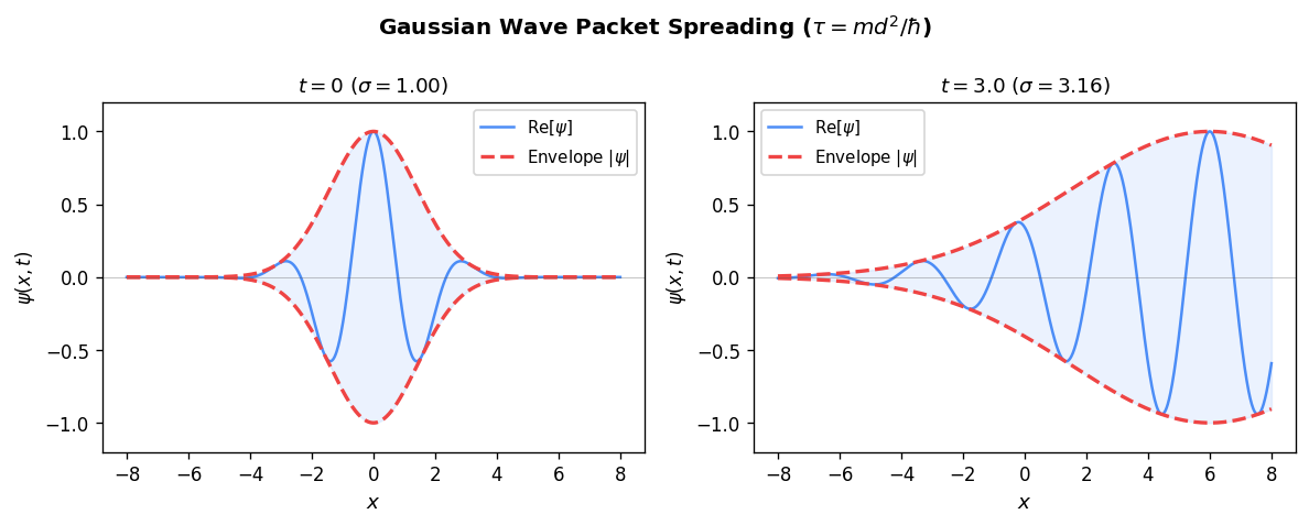
However, the quadratic dispersion \(\omega \propto k^2\) causes wave packet spreading. For the Gaussian packet with initial width \(\Delta x(0) = d/\sqrt{2}\), the width at time \(t\) is

\[\Delta x(t) = \frac{d}{\sqrt{2}}\sqrt{1 + \left(\frac{\hbar t}{md^2}\right)^2} = \frac{d}{\sqrt{2}}\sqrt{1 + (t/\tau)^2},\]

where \(\tau = md^2/\hbar\) is the spreading time scale. For an electron in a hydrogen atom, \(d \sim 0.5\) Å and \(\tau \sim 10^{-17}\) s — the packet spreads on an atomic timescale. For a macroscopic particle (say, a billiard ball with \(m \sim 0.1\) kg and \(d \sim 1\) mm), we get \(\tau \sim 10^{26}\) s, far larger than the age of the universe. Wave packet spreading is therefore a purely quantum phenomenon that is negligible for macroscopic objects but crucial at the atomic scale.

  Δx(t)
    |           ___________
    |          /
    |      ___/
    |   __/
    |__/
    |___________________________ t
    0       τ       2τ

The spreading is irreversible: once the wave packet spreads, the particle’s position becomes increasingly uncertain. This is not a limitation of measurement technology but a fundamental feature of quantum mechanics.

Section 2.2: The Time-Dependent Schrödinger Equation

3.1 The TDSE and Its Stationary Solutions

The central equation of quantum mechanics is the time-dependent Schrödinger equation (TDSE):

\[i\hbar\frac{\partial\Psi}{\partial t} = \hat{H}\Psi = \left(-\frac{\hbar^2}{2m}\frac{\partial^2}{\partial x^2} + U(x)\right)\Psi.\]

This is a first-order partial differential equation in time and second-order in space. It is linear, so any superposition of solutions is also a solution. The factor of \(i\) on the left-hand side is crucial: it ensures that probability is conserved (as we will prove in §3.5).

The TDSE is amenable to separation of variables whenever the potential \(U(x)\) does not depend on time. Suppose \(\Psi(x,t) = \psi(x)T(t)\). Substituting and dividing by \(\psi T\):

\[i\hbar\frac{\dot{T}}{T} = \frac{\hat{H}\psi}{\psi} = E,\]

where \(E\) is the separation constant, which will turn out to be the energy eigenvalue. The time equation gives \(T(t) = e^{-iEt/\hbar}\), and the spatial equation is the time-independent Schrödinger equation (TISE):

\[\hat{H}\psi = E\psi, \qquad \text{i.e.,} \qquad -\frac{\hbar^2}{2m}\psi'' + U(x)\psi = E\psi.\]

A solution \(\Psi_n(x,t) = \psi_n(x)e^{-iE_nt/\hbar}\) is called a stationary state because its probability density \(|\Psi_n|^2 = |\psi_n|^2\) is time-independent. Every observable computed from a stationary state is also time-independent. The general solution to the TDSE is a superposition of stationary states:

\[\Psi(x,t) = \sum_n C_n\,\psi_n(x)\,e^{-iE_nt/\hbar},\]

where the coefficients \(C_n\) are determined by the initial condition \(\Psi(x,0)\).

3.2 Sturm-Liouville Theory and Energy Spectra

The TISE \(\hat{H}\psi = E\psi\) is a Sturm-Liouville eigenvalue problem. The general theory of such equations guarantees three crucial properties for a particle moving under a confining potential (appropriate boundary conditions):

The nature of the energy spectrum depends on the shape of the potential:

• Bounded motion (the particle is classically confined): the eigenvalues form a discrete infinite sequence \(E_1 < E_2 < E_3 < \cdots \to \infty\).
• Unbounded motion (the particle can escape to infinity): the energy spectrum is continuous for \(E \ge E_{\min}\).
• Mixed spectrum: if a potential has a well that supports bound states at energies below some threshold and a continuum above, both types coexist.

    E
    |          _______________   continuum (E > 0)
    |         /
  0-|---------  - - - - - - -   threshold
    |
    |   ___  E_3
    |
    |   ___  E_2               discrete bound states
    |
    |   ___  E_1
    |
    |___________________________

This mixed spectrum appears in the hydrogen atom, where discrete bound states exist for \(E_n = -E_R/n^2 < 0\), and a continuum of ionized states for \(E > 0\).

3.3 The Free Particle and Dirac Notation

For a free particle (\(U=0\)), the TISE becomes \(-\frac{\hbar^2}{2m}\psi'' = E\psi\), with solutions \(\psi_p(x) = Ae^{ipx/\hbar}\) for energy \(E = p^2/(2m)\). These momentum eigenstates are not normalizable in the ordinary sense — they extend over all space. The correct normalization uses a delta function:

\[\psi_p(x) = \frac{1}{\sqrt{2\pi\hbar}}e^{ipx/\hbar}, \qquad \int_{-\infty}^{\infty}\psi_{p'}^*(x)\psi_p(x)\,dx = \delta(p-p').\]

This delta-function normalization replaces the Kronecker delta of the discrete case. The Dirac notation (bra-ket notation) provides an elegant way to write these relations:

\[\langle x'|x\rangle = \delta(x'-x), \qquad \langle p'|p\rangle = \delta(p'-p), \qquad \langle x|p\rangle = \frac{1}{\sqrt{2\pi\hbar}}e^{ipx/\hbar}.\]

Completeness relations (resolution of the identity) take the form

\[\int |x\rangle\langle x|\,dx = \hat{1}, \qquad \int |p\rangle\langle p|\,dp = \hat{1}.\]

These relations allow us to insert complete sets of states anywhere in an inner product, a technique that pervades the calculations of Chapter 6.

3.4 Boundary Conditions and the Particle in a Box

For a particle moving in a piecewise-constant potential, the solution in each region is a combination of exponentials (or sines and cosines), and these solutions must be joined at the interfaces using boundary conditions (BCs).

At a boundary where the potential has a finite jump (from \(U_L\) to \(U_R\) with \(|U_R - U_L| < \infty\)), both \(\psi\) and \(\psi'\) must be continuous — the wave function is \(C^1\). This follows from integrating the TISE across the interface and taking the jump to zero.

At a boundary where the potential is infinitely hard (a hard wall), only \(\psi\) must be continuous (and vanishes at the wall); \(\psi'\) may be discontinuous. This is because the delta-function-like derivative of an infinite potential step forces the derivative to jump.

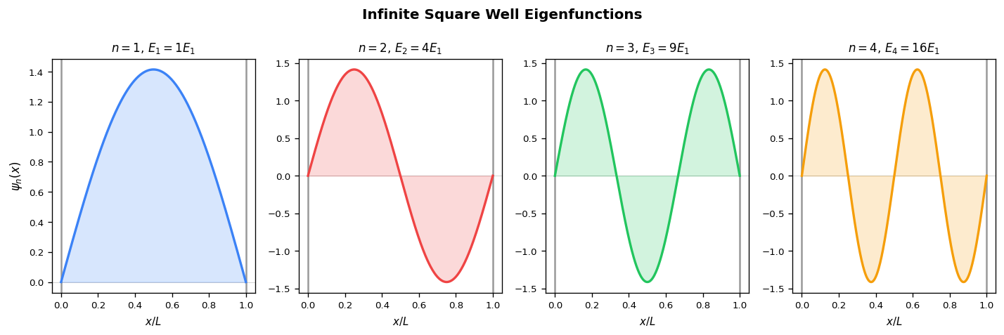
The particle in a box (PIB) is the prototypical quantum system. A particle of mass \(m\) is confined to \(0 \le x \le L\) by infinite walls: \(U=0\) inside and \(U=\infty\) outside. The BCs \(\psi(0)=\psi(L)=0\) select the stationary solutions

\[\psi_n(x) = \sqrt{\frac{2}{L}}\sin\!\left(\frac{n\pi x}{L}\right), \qquad E_n = \frac{\hbar^2}{2m}\left(\frac{n\pi}{L}\right)^2 = \frac{n^2\pi^2\hbar^2}{2mL^2},\]

for \(n = 1, 2, 3, \ldots\) The ground state (\(n=1\)) has energy \(E_1 = \pi^2\hbar^2/(2mL^2) > 0\) — the particle cannot be at rest, reflecting the zero-point energy demanded by the uncertainty principle. The energy levels scale as \(n^2\), so the spacing between adjacent levels grows with \(n\).

    E  |
       |                      ___   E_4 = 16 E_1
       |            ___       E_3 = 9 E_1
       |      ___             E_2 = 4 E_1
       |  ___                 E_1
    ___|________________________________
       0                    L

3.5 Probability Current and Norm Conservation

Multiply the TDSE by \(\Psi^*\) and subtract the complex conjugate equation multiplied by \(\Psi\):

\[i\hbar(\Psi^*\partial_t\Psi - \Psi\partial_t\Psi^*) = -\frac{\hbar^2}{2m}(\Psi^*\Psi'' - \Psi\Psi^{''*}) = -\frac{\hbar^2}{2m}\partial_x(\Psi^*\Psi' - \Psi\Psi'^*).\]

Dividing by \(i\hbar\) and rearranging yields the continuity equation:

\[\frac{\partial\rho}{\partial t} + \frac{\partial j}{\partial x} = 0,\]

where \(\rho = |\Psi|^2\) is the probability density and

\[j(x,t) = \frac{\hbar}{m}\,\text{Im}\!\left[\Psi^*\frac{\partial\Psi}{\partial x}\right] = \frac{\hbar}{2mi}\left(\Psi^*\frac{\partial\Psi}{\partial x} - \Psi\frac{\partial\Psi^*}{\partial x}\right)\]

is the probability current (probability flux). The continuity equation expresses local conservation of probability: if probability density decreases in some region, probability must be flowing out of that region. Integrating over all space and using vanishing BCs, we get \(\frac{d}{dt}\int|\Psi|^2\,dx = 0\), so the total probability is conserved.

3.6 Matrix Elements and Expectation Values

The expectation value of an observable \(\hat{A}\) in state \(\Psi\) is

\[\langle\hat{A}\rangle = \int\Psi^*\hat{A}\Psi\,dx = \langle\Psi|\hat{A}|\Psi\rangle.\]

For the PIB with \(\Psi(x,0) = \sum_n C_n\psi_n(x)\), the expectation value of energy is

\[\langle H\rangle = \sum_n |C_n|^2 E_n,\]

which is conserved in time since the \(|C_n|^2\) are time-independent (only the phases rotate).

The matrix element of operator \(\hat{A}\) between eigenstates \(\psi_m\) and \(\psi_n\) is

\[\langle m|\hat{A}|n\rangle = \int_0^L \psi_m^*(x)\hat{A}\psi_n(x)\,dx.\]

For the PIB, the matrix elements of \(\hat{x}\) and \(\hat{p}\) can be evaluated explicitly:

\[\langle n|\hat{x}|n\rangle = \frac{L}{2}, \qquad \langle n|\hat{p}|n\rangle = 0, \qquad \langle n|\hat{x}^2|n\rangle = L^2\left(\frac{1}{3} - \frac{1}{2n^2\pi^2}\right).\]

From these, the position and momentum uncertainties for the \(n\)-th PIB state are

\[\Delta x_n = \frac{L}{2\pi n}\sqrt{\frac{\pi^2 n^2}{3} - 2}, \qquad \Delta p_n = \frac{n\pi\hbar}{L},\]

giving \(\Delta x_n\Delta p_n > \hbar/2\) for all \(n \ge 1\), consistent with the Heisenberg uncertainty relation (with equality only in the limit \(n\to\infty\) up to corrections).

Chapter 3: Exactly Solvable Problems

Section 3.1: Scattering and Quantum Tunneling

4.1 Flux Conservation in Stationary Scattering States

For unbounded motion with a potential \(U(x)\) that is asymptotically constant as \(x\to\pm\infty\), we seek stationary scattering solutions. The probability current \(j(x,t) = j(x)\) is time-independent for a stationary state, and the continuity equation reduces to \(\partial_x j = 0\), meaning the current is constant throughout space. In particular, the probability flux to the left of the potential equals the flux to the right:

\[j_L = j_R.\]

This simple but profound statement is the basis for defining transmission and reflection coefficients.

4.2 Transmission and Reflection Coefficients

Consider a particle incident from the left with wave number \(k_L\) (energy \(E = \hbar^2 k_L^2/(2m)\) above the left-region potential \(U_L\)) and wave number \(k_R\) in the right region. The general form of the wave function is

\[\psi(x) = \begin{cases} Ae^{ik_L x} + Be^{-ik_L x} & x < 0\text{ (left region)}\\ Ce^{ik_R x} + De^{-ik_R x} & x > 0\text{ (right region)} \end{cases}\]

Setting \(D = 0\) (no wave incident from the right), \(A\) is the amplitude of the incident wave, \(B\) is the reflected amplitude, and \(C\) is the transmitted amplitude. The fluxes are

\[j_{\text{inc}} = \frac{\hbar k_L}{m}|A|^2, \quad j_{\text{ref}} = \frac{\hbar k_L}{m}|B|^2, \quad j_{\text{trans}} = \frac{\hbar k_R}{m}|C|^2.\]

The transmission probability and reflection probability are defined as

\[T = \frac{j_{\text{trans}}}{j_{\text{inc}}} = \frac{k_R}{k_L}\left|\frac{C}{A}\right|^2, \qquad R = \frac{j_{\text{ref}}}{j_{\text{inc}}} = \left|\frac{B}{A}\right|^2.\]

Conservation of probability flux requires \(T + R = 1\).

4.3 The Potential Step

The potential step is the simplest non-trivial scattering problem:

\[U(x) = \begin{cases} 0 & x < 0\\ V_0 & x > 0 \end{cases}\]

    U
    |            _______________
  V₀|           |
    |           |
    |___________|________________ x
                0

Case 1: \(E > V_0\) (above the step). Both regions admit oscillatory solutions. The matching conditions give

\[T = \frac{4k_1 k_2}{(k_1+k_2)^2}, \qquad R = \frac{(k_1-k_2)^2}{(k_1+k_2)^2},\]

where \(k_1 = \sqrt{2mE}/\hbar\) and \(k_2 = \sqrt{2m(E-V_0)}/\hbar\). Note that \(T < 1\) even when \(E > V_0\): a quantum particle is partially reflected by a step even when it has enough energy to surmount it. This has no classical analogue and is a direct consequence of wave mechanics.

Case 2: \(E < V_0\) (below the step). In the right region, the wave number becomes imaginary: \(k_2 = i\kappa\) with \(\kappa = \sqrt{2m(V_0-E)}/\hbar > 0\). The solution decays exponentially as \(e^{-\kappa x}\) — this is an evanescent wave. The reflection coefficient is \(R = 1\): the particle is totally reflected, but the wave function penetrates a distance \(\sim 1/\kappa\) into the classically forbidden region.

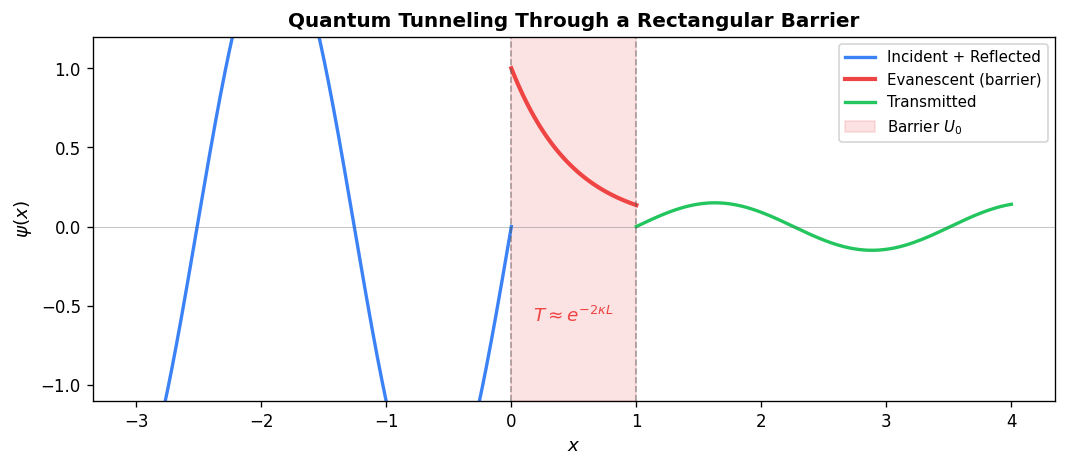
4.4 Rectangular Barrier and Quantum Tunneling

The rectangular barrier is the paradigmatic tunneling problem:

\[U(x) = \begin{cases} 0 & x < 0\\ U_0 & 0 \le x \le L\\ 0 & x > L \end{cases}\]

    U
    |     _________
  U₀|    |         |
    |    |         |
    |____|_________|_______ x
         0         L

For \(E < U_0\), the classically forbidden region \(0 \le x \le L\) admits solutions \(e^{\pm\kappa x}\) with \(\kappa = \sqrt{2m(U_0-E)}/\hbar\). By matching all four boundary conditions (continuity of \(\psi\) and \(\psi'\) at \(x=0\) and \(x=L\)), the transmission coefficient is

\[T = \frac{1}{\cosh^2(\kappa L) + \frac{(\kappa^2-k^2)^2}{4\kappa^2 k^2}\sinh^2(\kappa L)},\]

where \(k = \sqrt{2mE}/\hbar\). For an opaque barrier (\(\kappa L \gg 1\)), \(\cosh(\kappa L) \approx \sinh(\kappa L) \approx e^{\kappa L}/2\), so

\[T \approx \frac{16k^2\kappa^2}{(k^2+\kappa^2)^2}e^{-2\kappa L}.\]

The dominant factor \(e^{-2\kappa L}\) shows that tunneling is exponentially suppressed by both the barrier width \(L\) and the barrier height (which enters through \(\kappa\)). This exponential sensitivity explains why tunneling is dramatically important in some contexts (nuclear alpha decay, scanning tunnelling microscopy) but negligible in others (a billiard ball passing through a wall).

Resonant transmission. For \(E > U_0\), both regions have oscillatory solutions. The transmission is now \(T \le 1\), with \(T = 1\) (perfect transmission) at resonance energies

\[k'L = n\pi, \quad n = 1, 2, \ldots, \qquad \text{where } k' = \sqrt{2m(E-U_0)}/\hbar.\]

This Ramsauer-Townsend effect is the quantum analogue of anti-reflection coating in optics: at certain energies, the reflected waves from the two interfaces cancel exactly.

The delta-function barrier. In the limit \(L\to 0\), \(U_0\to\infty\) with \(U_0 L = \alpha/m\) fixed, the barrier becomes a delta function \(U(x) = \frac{\hbar^2\alpha}{2m}\delta(x)\). The transmission is

\[T = \frac{1}{1+\beta^2}, \qquad \beta = \frac{m\alpha}{\hbar^2 k},\]

where \(\beta\) is a dimensionless measure of the barrier strength relative to the particle’s kinetic energy.

4.5 The Transfer Matrix Method and Kronig-Penney Model

For a sequence of piecewise-constant potentials, matching boundary conditions at each interface produces a system of equations that can be organized into matrices. This transfer matrix method is especially powerful for periodic potentials.

In each region with wave number \(k\), the wave function is \(Ae^{ikx} + Be^{-ikx}\). A transfer matrix \(\underline{M}\) relates the amplitudes on the right to those on the left:

\[\begin{pmatrix}A_R\\B_R\end{pmatrix} = \underline{M}\begin{pmatrix}A_L\\B_L\end{pmatrix}.\]

The transfer matrix satisfies \(\det\underline{M} = 1\), and its elements obey \(M_{11}=M_{22}^*\), \(M_{12}=M_{21}^*\). The scattering matrix \(\underline{S}\) is unitary and symmetric, relating incoming to outgoing amplitudes.

For the Kronig-Penney model — a periodic array of identical barriers separated by free regions — Bloch’s theorem states that solutions must satisfy \(\psi(x+d) = e^{i\theta}\psi(x)\) for some phase \(\theta\). The propagator matrix over one period has trace

\[\text{Tr}(\underline{P}) = 2\left[\cos(kL) + \frac{\gamma}{kL}\sin(kL)\right],\]

where \(L\) is the period and \(\gamma\) parametrizes the barrier strength. Bloch solutions exist only when \(|\text{Tr}(\underline{P})| \le 2\) (since \(\theta\) must be real). This condition is satisfied for certain ranges of energy — the allowed energy bands — and violated for others — the energy gaps (band gaps).

  |Tr P|
    |     *       *     *
  2-|-  -   --  -   --     -  -   allowed band boundary
    |  * *  ** ** * ** *  * *
    |     ***    ***    ***
    |____________________________ E
       band gap   band gap

The Kronig-Penney model is the quantum mechanical basis for understanding the electronic band structure of crystalline solids. Electrons in allowed bands can propagate through the crystal and conduct electricity; those in band gaps cannot.

Section 3.2: Bound States in One Dimension

5.1 The Finite Potential Well

The finite potential well is more realistic than the infinite square well:

\[U(x) = \begin{cases} U_1 & x < 0 \\ 0 & 0 \le x \le L\\ U_2 & x > L \end{cases}\]

For \(0 < E < \min(U_1, U_2)\), we seek bound states. Inside the well, the solution oscillates; outside it decays exponentially. Matching boundary conditions at both interfaces gives a transcendental equation for the allowed energies. For the symmetric well (\(U_1 = U_2 = U_0\)):

\[kL = n\pi - \arcsin\!\left(\frac{\hbar k}{\sqrt{2mU_0}}\right) - \arcsin\!\left(\frac{\hbar k}{\sqrt{2mU_0}}\right), \quad n = 1, 2, \ldots\]

The number of bound states is finite, given approximately by

\[n_{\max} = \left\lceil\frac{\sqrt{2mU_0}\,L}{\pi\hbar}\right\rceil.\]

As \(U_0\to\infty\), the well becomes infinitely deep and we recover the particle-in-a-box levels. For a finite well, the wave function has tails that extend into the classically forbidden regions — the particle has a non-zero probability of being found outside the well.

        ψ₂(x)                   ψ₁(x)

  ~~~~~|  /\   |~~~~~     ~~~~~|  /\  |~~~~~
       | /  \  |               |/    \|
       |/    \ |
  _____|______\|_____     _____|______|_____
       0       L               0      L

5.2 The Simple Harmonic Oscillator

The simple harmonic oscillator (SHO) is the most important exactly-solvable problem in all of physics. Any smooth potential near a stable equilibrium can be approximated as a harmonic oscillator, so the SHO serves as the starting point for countless perturbative calculations. The potential is

\[U(x) = \frac{1}{2}\kappa x^2 = \frac{1}{2}m\omega^2 x^2, \qquad \omega = \sqrt{\kappa/m}.\]

Introducing the dimensionless variable \(\xi = \alpha x\) with \(\alpha = (m\omega/\hbar)^{1/2}\), the TISE becomes Hermite’s differential equation:

\[H'' - 2\xi H' + 2nH = 0,\]

where \(H(\xi)\) is the Hermite polynomial. For the solution to remain normalizable, the series must truncate, which requires the parameter \(n\) to be a non-negative integer. This gives the energy spectrum

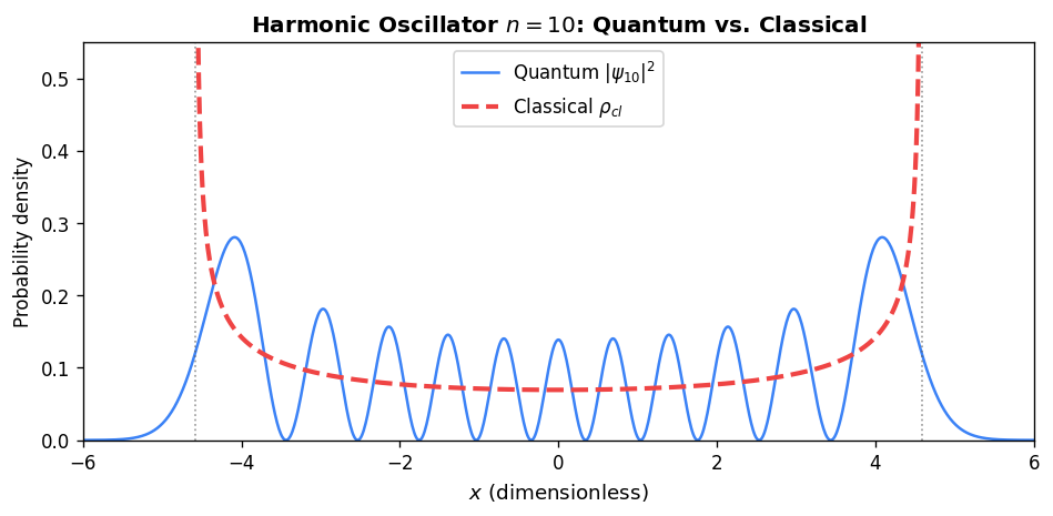
\[E_n = \hbar\omega\left(n + \frac{1}{2}\right), \qquad n = 0, 1, 2, \ldots\]

The equally spaced energy levels are a hallmark of the harmonic oscillator. The ground state energy \(E_0 = \frac{1}{2}\hbar\omega\) is the zero-point energy — the oscillator can never be at rest.

The eigenfunctions are

\[\psi_n(x) = C_n\, H_n(\alpha x)\, e^{-\alpha^2 x^2/2},\]

where \(H_n\) are the Hermite polynomials: \(H_0 = 1\), \(H_1 = 2\xi\), \(H_2 = 4\xi^2-2\), \(H_3 = 8\xi^3 - 12\xi\), etc. The normalization constant \(C_n = (\alpha/\sqrt{\pi})^{1/2}/\sqrt{2^n n!}\) can be derived from the generating function for Hermite polynomials.

    E
    |    ___    n=4, E=9ℏω/2
    |    ___    n=3, E=7ℏω/2
    |    ___    n=2, E=5ℏω/2
    |    ___    n=1, E=3ℏω/2
    |    ___    n=0, E=ℏω/2
    |__________________________  x
         U = mω²x²/2

The uncertainty relation for the SHO is saturated by the ground state: \(\Delta x\,\Delta p = \hbar(n+1/2) \ge \hbar/2\). For \(n=0\), the ground state is a Gaussian (as we saw in Chapter 2), achieving the minimum uncertainty \(\Delta x\,\Delta p = \hbar/2\). For higher \(n\), the uncertainty product grows linearly with \(n\), as the state becomes more spread out.

Chapter 4: The Mathematical Structure of Quantum Mechanics

Section 4.1: Hilbert Spaces, Operators, and the Axioms of Quantum Theory

The mathematical framework of quantum mechanics can be organized into four axioms. Rather than viewing these as postulates to be accepted uncritically, we should understand them as the minimal mathematical structure consistent with the experimental facts: the probabilistic nature of measurement, the superposition principle, and the uncertainty principle.

6.1 Axiom 1 — The Hilbert Space

A Hilbert space is a complex vector space equipped with an inner product \(\langle \cdot|\cdot\rangle\) that is complete (every Cauchy sequence converges). For one-dimensional quantum mechanics, \(\mathcal{H} = L^2(\mathbb{R})\) is the space of square-integrable functions, with inner product

\[\langle f|g\rangle = \int_{-\infty}^{\infty} f^*(x)\,g(x)\,dx.\]

The properties of the inner product are:

• Conjugate symmetry: \(\langle f|g\rangle = \langle g|f\rangle^*\)
• Linearity in second argument: \(\langle f|\alpha g + \beta h\rangle = \alpha\langle f|g\rangle + \beta\langle f|h\rangle\)
• Positive definiteness: \(\langle f|f\rangle \ge 0\), with equality iff \(f = 0\)

The norm of a state is \(\|f\| = \sqrt{\langle f|f\rangle}\). The Cauchy-Schwarz inequality states \(|\langle f|g\rangle| \le \|f\|\,\|g\|\), which is the key ingredient in proving the Heisenberg uncertainty relation.

Given a linearly independent set of vectors \(\{v_n\}\), the Gram-Schmidt procedure constructs an orthonormal basis: set \(e_1 = v_1/\|v_1\|\), then iteratively project out the components along previous basis vectors and normalize.

6.2 Axiom 2 — Hermitian Operators

The adjoint \(\hat{A}^\dagger\) of an operator \(\hat{A}\) is defined by \(\langle f|\hat{A}^\dagger|g\rangle = \langle g|\hat{A}|f\rangle^* = \langle\hat{A}f|g\rangle\). Note that:

• The derivative operator \(\hat{D} = \partial_x\) is anti-Hermitian: \(\hat{D}^\dagger = -\partial_x\). (Proof by integration by parts with vanishing boundary conditions.)
• The momentum operator \(\hat{p} = \frac{\hbar}{i}\partial_x\) is Hermitian: \(\hat{p}^\dagger = \frac{\hbar}{i}(-\partial_x)(-1) = \hat{p}\). ✓
• Products satisfy \((\hat{A}\hat{B})^\dagger = \hat{B}^\dagger\hat{A}^\dagger\) — the adjoint reverses the order of operators.

The expectation value of an observable in state \(|f\rangle\) is \(\langle A\rangle = \langle f|\hat{A}|f\rangle\). Hermiticity guarantees that this is real: \(\langle A\rangle^* = \langle f|\hat{A}^\dagger|f\rangle = \langle f|\hat{A}|f\rangle = \langle A\rangle\).

6.3 Axiom 3 — Measurement and Eigenvalues

Two fundamental theorems follow from the Hermitian nature of observables:

Proof of real eigenvalues. Suppose \(\hat{A}|\psi\rangle = a|\psi\rangle\). Then \(\langle\psi|\hat{A}|\psi\rangle = a\langle\psi|\psi\rangle\). But by Hermiticity, \(\langle\psi|\hat{A}|\psi\rangle = \langle\hat{A}\psi|\psi\rangle = a^*\langle\psi|\psi\rangle\). So \(a = a^*\), meaning \(a\) is real. \(\square\)

Proof of orthogonality. Suppose \(\hat{A}|\psi_m\rangle = a_m|\psi_m\rangle\) and \(\hat{A}|\psi_n\rangle = a_n|\psi_n\rangle\) with \(a_m \ne a_n\). Then

\[\langle\psi_m|\hat{A}|\psi_n\rangle = a_n\langle\psi_m|\psi_n\rangle = \langle\hat{A}\psi_m|\psi_n\rangle = a_m\langle\psi_m|\psi_n\rangle.\]

So \((a_n - a_m)\langle\psi_m|\psi_n\rangle = 0\). Since \(a_n \ne a_m\), we must have \(\langle\psi_m|\psi_n\rangle = 0\). \(\square\)

For continuous spectra, the eigenvalues form a continuum and the eigenfunctions are normalized with a delta function rather than a Kronecker delta. The probability of measuring a value in the interval \([a,a+da]\) is proportional to \(|\langle\psi_a|f\rangle|^2\,da\).

6.4 Axiom 4 — Time Evolution

The time-evolution operator \(\hat{U}(t) = e^{-i\hat{H}t/\hbar}\) is unitary: \(\hat{U}^\dagger\hat{U} = \hat{1}\). Unitarity is equivalent to the conservation of probability: \(\|f(t)\| = \|f(0)\| = 1\) for all time.

6.5 Commutators and the Uncertainty Principle

The commutator of two operators \(\hat{A}\) and \(\hat{B}\) is \([\hat{A},\hat{B}] = \hat{A}\hat{B} - \hat{B}\hat{A}\). Several fundamental commutators:

\[[\hat{x},\hat{p}] = i\hbar, \qquad [\hat{H},\hat{x}] = -\frac{i\hbar\hat{p}}{m}, \qquad [\hat{H},\hat{p}] = -\frac{\hbar}{i}\frac{dU}{dx}.\]

The first identity \([\hat{x},\hat{p}] = i\hbar\) (the canonical commutation relation) is the quantum counterpart of the classical Poisson bracket \(\{x,p\}=1\). It encodes the fundamental incompatibility of position and momentum measurements.

Compatible observables. Two observables \(\hat{A}\) and \(\hat{B}\) are compatible (simultaneously measurable) if and only if \([\hat{A},\hat{B}] = 0\). Compatible operators share a common eigenbasis — states that are simultaneously eigenstates of both operators. A complete set of commuting observables (CSCO) is the minimal set of mutually commuting operators whose simultaneous eigenvalues label the states of the system uniquely.

The parity operator \(\hat{P}\) acts as \(\hat{P}\psi(x) = \psi(-x)\). For a symmetric potential \(U(x) = U(-x)\), we have \([\hat{H},\hat{P}] = 0\), so energy eigenstates can be chosen to have definite parity. The SHO eigenfunctions alternate: \(\psi_n(-x) = (-1)^n\psi_n(x)\), so even \(n\) have even parity and odd \(n\) have odd parity.

The Heisenberg Uncertainty Relation. The general form of the uncertainty relation follows from the algebraic properties of Hilbert spaces.

Proof. Define the shifted operators \(\tilde{A} = \hat{A} - \langle\hat{A}\rangle\) and \(\tilde{B} = \hat{B} - \langle\hat{B}\rangle\) (note \([\tilde{A},\tilde{B}] = [\hat{A},\hat{B}]\)). Consider the non-Hermitian operator \(\hat{C} = \tilde{A} + i\lambda\tilde{B}\) for real \(\lambda\). Then

\[\|\hat{C}|f\rangle\|^2 = \langle f|\hat{C}^\dagger\hat{C}|f\rangle = (\Delta A)^2 + \lambda^2(\Delta B)^2 + i\lambda\langle[\tilde{A},\tilde{B}]\rangle \ge 0.\]

This is a quadratic function \(F(\lambda) = (\Delta B)^2\lambda^2 + i\lambda\langle[\hat{A},\hat{B}]\rangle + (\Delta A)^2\) that is non-negative for all real \(\lambda\). Its discriminant must be non-positive:

\[(i\langle[\hat{A},\hat{B}]\rangle)^2 - 4(\Delta A)^2(\Delta B)^2 \le 0,\]

which gives \((\Delta A)^2(\Delta B)^2 \ge \frac{1}{4}|\langle[\hat{A},\hat{B}]\rangle|^2\). Taking square roots yields the result. \(\square\)

For position and momentum, \([\hat{x},\hat{p}] = i\hbar\), so \(\Delta x\,\Delta p \ge \hbar/2\). The bound is achieved by Gaussian wave packets, as we saw in Chapter 2.

6.6 The Equation of Motion and Ehrenfest’s Theorem

For an observable \(\hat{A}\) that may depend explicitly on time, the equation of motion for its expectation value is

\[\frac{d}{dt}\langle\hat{A}\rangle = \frac{i}{\hbar}\langle[\hat{H},\hat{A}]\rangle + \left\langle\frac{\partial\hat{A}}{\partial t}\right\rangle.\]

This is Ehrenfest’s theorem. Using \([\hat{H},\hat{x}] = -i\hbar\hat{p}/m\) and \([\hat{H},\hat{p}] = -\frac{\hbar}{i}\frac{dU}{dx}\):

\[\frac{d\langle x\rangle}{dt} = \frac{\langle p\rangle}{m}, \qquad \frac{d\langle p\rangle}{dt} = -\left\langle\frac{dU}{dx}\right\rangle.\]

These are Newton’s equations for the expectation values — quantum mechanics reduces to classical mechanics in the sense of expectation values. The subtle point is that \(\langle dU/dx\rangle \approx dU(\langle x\rangle)/dx\) only when the wave packet is narrow compared to the scale on which \(U\) varies; in general, quantum corrections appear.

Chapter 5: Quantum Mechanics in Three Dimensions

Section 5.1: Central Potentials and the Hydrogen Atom

7.1 Separable Solutions in Cartesian Coordinates

In three dimensions, the Hamiltonian for a particle in a potential \(U(\vec{r})\) is

\[\hat{H} = -\frac{\hbar^2}{2m}\nabla^2 + U(\vec{r}) = -\frac{\hbar^2}{2m}\left(\frac{\partial^2}{\partial x^2}+\frac{\partial^2}{\partial y^2}+\frac{\partial^2}{\partial z^2}\right) + U(\vec{r}).\]

When the potential separates as \(U(\vec{r}) = U_x(x) + U_y(y) + U_z(z)\), the wave function separates as \(\psi(\vec{r}) = X(x)Y(y)Z(z)\), and the energy is additive: \(E = E_x + E_y + E_z\). The 3D particle in a box (a rectangular box with sides \(L_x, L_y, L_z\)) has energy levels

\[E_{n_xn_yn_z} = \frac{\hbar^2\pi^2}{2m}\left(\frac{n_x^2}{L_x^2}+\frac{n_y^2}{L_y^2}+\frac{n_z^2}{L_z^2}\right).\]

For a cubic box (\(L_x = L_y = L_z = L\)), the energy levels exhibit degeneracy: different combinations \((n_x,n_y,n_z)\) can give the same total energy. For example, the first excited level has energy \(E_{211} = E_{121} = E_{112}\) — threefold degenerate.

7.2 Central Potentials and Angular Momentum

A central potential depends only on the radial distance: \(U(\vec{r}) = U(r)\). Such potentials are spherically symmetric, meaning the Hamiltonian commutes with all three components of angular momentum \(\hat{\vec{L}} = \vec{r}\times\hat{\vec{p}}\).

In spherical coordinates \((r,\theta,\phi)\), the Laplacian separates as

\[\nabla^2 = \frac{1}{r^2}\frac{\partial}{\partial r}\left(r^2\frac{\partial}{\partial r}\right) - \frac{\hat{L}^2}{\hbar^2 r^2},\]

where the angular momentum squared operator is

\[\hat{L}^2 = -\hbar^2\left[\frac{1}{\sin\theta}\frac{\partial}{\partial\theta}\left(\sin\theta\frac{\partial}{\partial\theta}\right)+\frac{1}{\sin^2\theta}\frac{\partial^2}{\partial\phi^2}\right].\]

The key commutation relations are

\[[\hat{L}^2,\hat{H}] = 0, \quad [\hat{L}_z,\hat{H}] = 0, \quad [\hat{L}^2,\hat{L}_z] = 0, \quad [\hat{L}_x,\hat{L}_y] = i\hbar\hat{L}_z\]

(and cyclic permutations of the last). The first three relations mean that \(\{\hat{H},\hat{L}^2,\hat{L}_z\}\) forms a CSCO for a central potential — we can find simultaneous eigenstates of all three operators. The last relation shows that \(\hat{L}_x\) and \(\hat{L}_y\) are incompatible: their uncertainty relation gives \(\Delta L_x\,\Delta L_y \ge \frac{\hbar}{2}|\langle\hat{L}_z\rangle|\).

7.3 Separation of Variables

For a central potential, we seek solutions \(\psi(r,\theta,\phi) = R(r)Y(\theta,\phi)\). Substituting into the TISE:

\[\left[-\frac{\hbar^2}{2m}\frac{1}{r^2}\frac{d}{dr}\left(r^2\frac{d}{dr}\right) + \frac{\hbar^2 l(l+1)}{2mr^2} + U(r)\right]R = ER,\]

where the separation constant is \(\hbar^2 l(l+1)\) (to be justified below), and the angular equation is

\[\hat{L}^2 Y = \hbar^2 l(l+1)\,Y.\]

The radial equation has an effective potential \(U_{\text{eff}}(r) = U(r) + \hbar^2 l(l+1)/(2mr^2)\): the centrifugal barrier \(\sim l(l+1)/r^2\) adds to the physical potential, pushing particles with higher angular momentum away from the origin.

7.4 Spherical Harmonics

The angular equation \(\hat{L}^2 Y_{lm} = \hbar^2 l(l+1)Y_{lm}\) is solved by separation \(Y(\theta,\phi) = \Theta(\theta)\Phi(\phi)\).

Azimuthal equation. The \(\phi\)-equation is \(-\partial_\phi^2\Phi = m^2\Phi\), with solutions \(\Phi_m(\phi) = e^{im\phi}/\sqrt{2\pi}\). Single-valuedness requires \(e^{im\cdot 2\pi} = 1\), so \(m\) must be an integer: \(m = 0, \pm 1, \pm 2, \ldots\) The quantum number \(m\) is called the magnetic quantum number (because it determines the splitting in a magnetic field).

Polar equation. Substituting \(w = \cos\theta\) transforms the \(\theta\)-equation into the Legendre equation:

\[(1-w^2)P'' - 2wP' + \left[l(l+1) - \frac{m^2}{1-w^2}\right]P = 0.\]

For \(m=0\), the solutions regular at \(w = \pm 1\) (i.e., at the poles \(\theta = 0, \pi\)) are the Legendre polynomials, generated by Rodrigues’ formula:

\[P_l(w) = \frac{1}{2^l l!}\frac{d^l}{dw^l}(w^2-1)^l.\]

The series for \(P_l\) terminates (giving a polynomial of degree \(l\)) only when \(l\) is a non-negative integer. The first few are:

\[P_0 = 1, \quad P_1 = w = \cos\theta, \quad P_2 = \frac{3w^2-1}{2} = \frac{3\cos^2\theta-1}{2}, \quad P_3 = \frac{5w^3-3w}{2}.\]

For \(m\ne 0\), the solutions are the associated Legendre functions:

\[P_l^m(w) = (1-w^2)^{|m|/2}\frac{d^{|m|}}{dw^{|m|}}P_l(w),\]

and the constraint \(-l \le m \le l\) emerges from the requirement that \(P_l^m\) be non-singular.

The normalized spherical harmonics are

\[Y_{lm}(\theta,\phi) = (-1)^{(m+|m|)/2}\sqrt{\frac{2l+1}{4\pi}\frac{(l-m)!}{(l+m)!}}\,P_l^m(\cos\theta)\,e^{im\phi}.\]

They satisfy the eigenvalue equations

\[\hat{L}^2 Y_{lm} = \hbar^2 l(l+1)\,Y_{lm}, \qquad \hat{L}_z Y_{lm} = \hbar m\,Y_{lm},\]

and are orthonormal: \(\langle Y_{l'm'}|Y_{lm}\rangle = \delta_{ll'}\delta_{mm'}\).

The first few spherical harmonics are:

\(l\)	\(m\)	\(Y_{lm}(\theta,\phi)\)
0	0	\(\frac{1}{\sqrt{4\pi}}\)
1	0	\(\sqrt{\frac{3}{4\pi}}\cos\theta\)
1	±1	\(\mp\sqrt{\frac{3}{8\pi}}\sin\theta\,e^{\pm i\phi}\)
2	0	\(\sqrt{\frac{5}{16\pi}}(3\cos^2\theta-1)\)
2	±1	\(\mp\sqrt{\frac{15}{8\pi}}\sin\theta\cos\theta\,e^{\pm i\phi}\)
2	±2	\(\sqrt{\frac{15}{32\pi}}\sin^2\theta\,e^{\pm 2i\phi}\)

The angular distribution \(|Y_{lm}(\theta,\phi)|^2\) is a function only of \(\theta\). Schematically, the shapes are:

  Y₀₀: sphere       Y₁₀: dumbbell     Y₂₀: double dumbbell

     *               *   *              *  *   *  *
    ***             * * * *            * * * * * *
     *               *   *              *  *   *  *
  isotropic        along z-axis       elongated along z

The \(l=0\) state is spherically symmetric; \(l=1\) states have lobes along the Cartesian axes; higher \(l\) states have increasingly complex angular structures.

7.5 The Rigid Rotator

A diatomic molecule can be modelled as a rigid rotator — two masses at fixed distance \(d\), rotating about their centre of mass. The Hamiltonian is purely rotational:

\[\hat{H} = \frac{\hat{L}^2}{2I}, \qquad I = \mu d^2,\]

where \(I\) is the moment of inertia and \(\mu\) is the reduced mass. Since \([\hat{H},\hat{L}^2] = [\hat{H},\hat{L}_z] = 0\), the eigenfunctions are spherical harmonics and the energy levels are

\[E_l = \frac{\hbar^2 l(l+1)}{2I}, \qquad l = 0, 1, 2, \ldots\]

Each level is \((2l+1)\)-fold degenerate (for \(m = -l, \ldots, +l\)). The spacing between adjacent levels increases: \(E_{l+1} - E_l = \hbar^2(l+1)/I\). Rotational transitions of molecules (in the microwave spectrum) thus produce equally spaced lines whose spacing reveals the moment of inertia and hence the bond length.

7.6 The Hydrogen Atom

The hydrogen atom is the central exactly-solvable problem of atomic physics. It consists of a proton and an electron interacting via the Coulomb potential \(U(r) = -k_c Ze^2/r\) (where \(Z=1\) for hydrogen). Working in the centre-of-mass frame, the problem reduces to a single particle of reduced mass \(\mu = m_e m_p/(m_e+m_p) \approx m_e\) in a central Coulomb potential.

The radial equation. After separating the angular part (which gives spherical harmonics as above), the radial equation for \(R_{nl}(r)\) is

\[-\frac{\hbar^2}{2\mu}\frac{d^2w}{dr^2} + \left(-k_c\frac{Ze^2}{r} + \frac{\hbar^2 l(l+1)}{2\mu r^2}\right)w = Ew,\]

where \(w(r) = rR(r)\). The effective potential for each \(l\) is:

    U_eff
    |                      ← U_eff for l>0
    |              ____----
    |          ---/         ← centrifugal barrier
    |       --/
  --|-  ---/                ← l=0 (no barrier)
    |   -ke²/r
    |___________________________ r
          r_min    r_0

Introducing the dimensionless variable \(\rho = 2\kappa r\) with \(\kappa = \sqrt{-2\mu E}/\hbar\) (valid for bound states, \(E < 0\)), and a series solution for the regular part of the radial function, one finds that the series must truncate to ensure normalizability. This truncation condition gives the principal quantum number \(n = 1, 2, 3, \ldots\), with the constraint \(l \le n-1\), and yields the energy levels:

\[E_n = -\frac{Z^2 E_R}{n^2}, \qquad E_R = \frac{k_c^2\mu e^4}{2\hbar^2} \approx 13.6\text{ eV}.\]

Here \(E_R\) is the Rydberg energy. The natural length scale is the Bohr radius:

\[a_B = \frac{\hbar^2}{k_c\mu e^2} \approx 0.529\text{ Å}.\]

The radial eigenfunctions involve associated Laguerre polynomials \(L_{n-l-1}^{2l+1}(\rho)\):

\[R_{nl}(r) = N_{nl}\left(\frac{2Zr}{na_B}\right)^l e^{-Zr/(na_B)}L_{n-l-1}^{2l+1}\!\left(\frac{2Zr}{na_B}\right),\]

where \(N_{nl}\) is a normalization constant.

Quantum numbers and degeneracy. Each state is labelled by three quantum numbers:

• \(n = 1, 2, 3, \ldots\) (principal): determines energy
• \(l = 0, 1, \ldots, n-1\) (orbital angular momentum): determines angular shape
• \(m = -l, \ldots, +l\) (magnetic): determines orientation

The total degeneracy of level \(n\) is \(\sum_{l=0}^{n-1}(2l+1) = n^2\). (This \(n^2\)-fold degeneracy is specific to the Coulomb potential and is related to an extra symmetry — the Runge-Lenz vector.)

Spectroscopic notation. Orbital angular momentum states are labelled by letters: \(l=0,1,2,3,\ldots\) is denoted \(s,p,d,f,\ldots\) So the ground state \((n=1,l=0)\) is 1s; the first excited level includes 2s (\(l=0\)) and 2p (\(l=1\)), etc.

Energy level diagram:

    E (eV)
    0  ________________   n = ∞ (continuum)
       ________________   n = 4, E = -0.85 eV
       ________________   n = 3, E = -1.51 eV


       ________________   n = 2, E = -3.40 eV




       ________________   n = 1, E = -13.6 eV  (ground state)

The Rydberg formula for spectral lines:

\[\frac{1}{\lambda} = Z^2 R_\infty\left(\frac{1}{n_f^2} - \frac{1}{n_i^2}\right),\]

where \(R_\infty = E_R/(hc) \approx 1.097\times 10^7\) m\(^{-1}\) is the Rydberg constant. Series of lines with \(n_f=1\) (Lyman, UV), \(n_f=2\) (Balmer, visible), \(n_f=3\) (Paschen, IR) are all observed.

Expectation values. For the ground state (\(n=1,l=0,m=0\)):

\[\psi_{100} = \frac{1}{\sqrt{\pi}a_B^3}e^{-r/a_B}, \qquad \langle r\rangle = \frac{3}{2}a_B, \qquad \Delta r = \frac{\sqrt{3}}{2}a_B.\]

The virial theorem gives \(\langle E_k\rangle = -E_n\) and \(\langle U\rangle = 2E_n\), consistent with \(E_n = \langle E_k\rangle + \langle U\rangle = -E_R/n^2\).

7.7 Magnetic Effects and Orbital Angular Momentum

In a uniform magnetic field \(\vec{B} = B_0\hat{z}\), the orbital magnetic dipole moment of the electron is

\[\hat{\vec{\mu}}_L = -\frac{|e|}{2m_e c}\hat{\vec{L}}.\]

The interaction Hamiltonian is \(\hat{H}_{\text{mag}} = -\hat{\vec{\mu}}_L\cdot\vec{B} = \frac{|e|B_0}{2m_e c}\hat{L}_z = \omega_L\hat{L}_z\), where

\[\omega_L = \frac{|e|B_0}{2m_e c} = \frac{\mu_B B_0}{\hbar}\]

is the Larmor frequency, and \(\mu_B = |e|\hbar/(2m_e c) \approx 9.27\times 10^{-24}\) J/T is the Bohr magneton. The perturbed energy levels are

\[E_{nlm} = E_n + \hbar\omega_L m, \qquad m = -l,\ldots,+l.\]

The \((2l+1)\)-fold degenerate level \(E_n\) splits into \(2l+1\) equally spaced levels. This is the normal Zeeman effect (the anomalous Zeeman effect requires spin, treated in Chapter 8).

7.8 Ladder Operators for Angular Momentum

The angular momentum operators can be combined into raising and lowering operators:

\[\hat{L}_\pm = \hat{L}_x \pm i\hat{L}_y.\]

These satisfy the commutation relations

\[[\hat{L}^2, \hat{L}_\pm] = 0, \qquad [\hat{L}_z, \hat{L}_\pm] = \pm\hbar\hat{L}_\pm.\]

The second relation shows that \(\hat{L}_\pm\) raises (or lowers) the magnetic quantum number by one: if \(\hat{L}_z Y_{lm} = \hbar m Y_{lm}\), then \(\hat{L}_z(\hat{L}_\pm Y_{lm}) = \hbar(m\pm 1)(\hat{L}_\pm Y_{lm})\). Explicitly:

\[\hat{L}_\pm Y_{lm} = C_{lm}^\pm Y_{l,m\pm1}, \qquad C_{lm}^\pm = \hbar\sqrt{l(l+1)-m(m\pm1)}.\]

The ladder must terminate: there is a maximum \(m_{\max}\) such that \(\hat{L}_+Y_{l,m_{\max}} = 0\), and a minimum \(m_{\min}\) such that \(\hat{L}_-Y_{l,m_{\min}} = 0\). From these conditions one can show that \(m_{\max} = l\), \(m_{\min} = -l\), and crucially that \(l\) must be either an integer or a half-integer.

Integer values of \(l\) correspond to bosons (orbital angular momentum, photons); half-integer values correspond to fermions (particles with spin-1/2). The electron, as we discover in the next chapter, has spin \(s = 1/2\) — a half-integer angular momentum with no classical analogue.

Chapter 6: Spin

Section 6.1: Electron Spin and the Pauli Theory

8.1 The Stern-Gerlach Experiment

In 1922, Stern and Gerlach passed a beam of silver atoms through an inhomogeneous magnetic field. Classical physics predicts that the magnetic dipole moments of the atoms should be continuously distributed, giving a continuous spread in deflection. Instead, the beam split into exactly two discrete spots.

The explanation: the silver atom has one outer electron in an \(l=0\) (s-orbital) state, so it has zero orbital angular momentum and hence zero orbital magnetic moment. The observed splitting must therefore arise from an intrinsic spin angular momentum \(\hat{\vec{S}}\) of the electron. The two spots correspond to spin projection \(m_s = +1/2\) (“spin up,” \(\uparrow\)) and \(m_s = -1/2\) (“spin down,” \(\downarrow\)).

In the two-dimensional spin space, the spin states are represented as column vectors called spinors:

\[\chi_+ = \begin{pmatrix}1\\0\end{pmatrix} \quad (\text{spin up, } m_s=+1/2), \qquad \chi_- = \begin{pmatrix}0\\1\end{pmatrix} \quad (\text{spin down, } m_s=-1/2).\]

A general spin state is \(\chi = c_+\chi_+ + c_-\chi_-\) with \(|c_+|^2 + |c_-|^2 = 1\).

The Hamiltonian for spin in a magnetic field \(\vec{B} = B_0\hat{z}\) includes a factor of \(g \approx 2\) (the electron \(g\)-factor, measured experimentally):

\[\hat{H}_s = g\frac{|e|B_0}{2m_e c}\hat{S}_z = \omega_L\hbar\hat{\sigma}_z,\]

where \(\omega_L = \mu_B B_0/\hbar\) is the Larmor frequency and \(\hat{\sigma}_z = \hat{S}_z/(\hbar/2)\) is the dimensionless spin operator.

8.2 Pauli Spin Matrices

The spin operators \(\hat{S}_i = (\hbar/2)\hat{\sigma}_i\) are represented in the \(\{\chi_+,\chi_-\}\) basis by the Pauli spin matrices:

\[\hat{\sigma}_x = \begin{pmatrix}0&1\\1&0\end{pmatrix}, \qquad \hat{\sigma}_y = \begin{pmatrix}0&-i\\i&0\end{pmatrix}, \qquad \hat{\sigma}_z = \begin{pmatrix}1&0\\0&-1\end{pmatrix}.\]

These satisfy remarkable algebraic identities. First, the squares:

\[\hat{\sigma}_x^2 = \hat{\sigma}_y^2 = \hat{\sigma}_z^2 = \hat{1}.\]

Second, the commutation relations (same as orbital angular momentum with \(\hbar\to 2\)):

\[[\hat{\sigma}_x,\hat{\sigma}_y] = 2i\hat{\sigma}_z, \quad [\hat{\sigma}_y,\hat{\sigma}_z] = 2i\hat{\sigma}_x, \quad [\hat{\sigma}_z,\hat{\sigma}_x] = 2i\hat{\sigma}_y.\]

Third, the anticommutation relations:

\[\{\hat{\sigma}_i,\hat{\sigma}_j\} = \hat{\sigma}_i\hat{\sigma}_j + \hat{\sigma}_j\hat{\sigma}_i = 2\delta_{ij}\hat{1}.\]

Additional properties: each Pauli matrix has trace 0 and determinant \(-1\), and satisfies \(\hat{\sigma}_i^\dagger = \hat{\sigma}_i\) (Hermitian).

The eigenvalues of \(\hat{\sigma}_x\) are \(\pm 1\), with eigenvectors \(\frac{1}{\sqrt{2}}(1,\pm1)^T\). A spin measured along an arbitrary direction \(\hat{u} = (\sin\theta\cos\phi,\sin\theta\sin\phi,\cos\theta)\) is represented by

\[\hat{\sigma}_u = \hat{u}\cdot\hat{\vec{\sigma}} = \begin{pmatrix}\cos\theta & \sin\theta e^{-i\phi}\\\sin\theta e^{i\phi} & -\cos\theta\end{pmatrix},\]

with eigenvalues \(\pm 1\) and eigenvectors

\[\chi_+ = \begin{pmatrix}\cos(\theta/2)\\e^{i\phi}\sin(\theta/2)\end{pmatrix}, \qquad \chi_- = \begin{pmatrix}\sin(\theta/2)\\-e^{i\phi}\cos(\theta/2)\end{pmatrix}.\]

8.3 Spin Precession in a Magnetic Field

For an electron initially in the spin state \(\chi = \cos(\theta/2)\chi_+ + \sin(\theta/2)e^{i\phi_0}\chi_-\), the time-dependent Schrödinger equation with \(\hat{H}_s = \mu_B B_0\hat{\sigma}_z\) gives

\[\chi(t) = \cos(\theta/2)\,e^{-i\omega_L t}\chi_+ + \sin(\theta/2)\,e^{i(\phi_0+\omega_L t)}\chi_-.\]

The expectation values of the spin components are

\[\langle\hat{S}_x\rangle = \frac{\hbar}{2}\sin\theta\cos(2\omega_L t + \phi_0), \quad \langle\hat{S}_y\rangle = -\frac{\hbar}{2}\sin\theta\sin(2\omega_L t + \phi_0), \quad \langle\hat{S}_z\rangle = \frac{\hbar}{2}\cos\theta.\]

This describes Larmor precession: the spin vector precesses around the \(z\)-axis (the field direction) at frequency \(2\omega_L\). The \(z\)-component is constant (energy is conserved), while the transverse components oscillate. This precession is directly observed in NMR (nuclear magnetic resonance) and MRI.

       z
       |  B₀
       |  ↑
       | /
       |/θ  ←  spin vector traces out a cone
       +------------- x
      /
     / (precesses at 2ω_L)
    y

8.4 The Weak Zeeman Effect

When an electron is bound in an atom and simultaneously subject to an external magnetic field, both orbital motion and spin contribute to the interaction. The correct quantum Hamiltonian follows from the minimal coupling prescription: replace the classical momentum \(\vec{p}\) with \(\vec{p} - (e/c)\vec{A}\), where \(\vec{A}\) is the vector potential.

The resulting quantum Hamiltonian is

\[\hat{H}_Q = \frac{1}{2m_e}\left(\hat{\vec{p}} - \frac{e}{c}\vec{A}\right)^2 + e\phi(\vec{r}) = \frac{\hat{p}^2}{2m_e} - \frac{e}{m_e c}\vec{A}\cdot\hat{\vec{p}} + \frac{e^2\vec{A}^2}{2m_e c^2} + e\phi(\vec{r}).\]

In the Coulomb gauge \(\nabla\cdot\vec{A} = 0\), the operators \(\hat{p}\) and \(\vec{A}\) commute, simplifying the expression. For a uniform field \(\vec{B} = (0,0,B_0)\), the symmetric gauge gives \(\vec{A} = \frac{1}{2}(\vec{B}\times\vec{r}) = \frac{B_0}{2}(-y,x,0)\). A key identity from vector calculus gives

\[\vec{A}\cdot\hat{\vec{p}} = \frac{1}{2}(\vec{B}\times\vec{r})\cdot\hat{\vec{p}} = \frac{1}{2}\vec{B}\cdot(\vec{r}\times\hat{\vec{p}}) = \frac{1}{2}\vec{B}\cdot\hat{\vec{L}}.\]

For a weak magnetic field, we neglect the quadratic term \(\propto\vec{A}^2\) and obtain the orbital Hamiltonian

\[\hat{H}_{\text{orb}} = \underbrace{-\frac{\hbar^2}{2m_e}\nabla^2 - k_c\frac{e^2}{r}}_{\hat{H}_0} - \frac{e}{2m_e c}\vec{B}\cdot\hat{\vec{L}} = \hat{H}_0 + \omega_L\hat{L}_z.\]

Including the spin interaction \(\hat{H}_s = \omega_L\hbar\hat{\sigma}_z\), and extending \(\hat{H}_{\text{orb}}\) to act on the two-component spinor space, the full Zeeman Hamiltonian is

\[\hat{H}_Z = \left(\hat{H}_0 + \omega_L\hat{L}_z\right)\hat{1} + \hbar\omega_L\hat{\sigma}_z.\]

8.5 Spinor Eigenstates and Level Splitting

Since \(\hat{S}_z\) commutes with \(\hat{H}_0 + \omega_L\hat{L}_z\), the quantum number \(m_s = \pm 1/2\) is a good quantum number. The full hydrogen atom state in a magnetic field is a spinor:

\[\boldsymbol{\psi}(r,\theta,\phi) = \begin{pmatrix}\psi_+(r,\theta,\phi)\\\psi_-(r,\theta,\phi)\end{pmatrix} = c_+\psi_{nlm}(\vec{r})\chi_+ + c_-\psi_{nlm}(\vec{r})\chi_-.\]

The normalization requires \(|c_+|^2 + |c_-|^2 = 1\), with \(|c_\pm|^2\) being the probability that the spin is up or down regardless of position. The TISE for \(\hat{H}_Z\) decouples into two equations:

\[\hat{H}_0\psi_+ + \omega_L(\hat{L}_z + \hbar)\psi_+ = E\psi_+, \qquad \hat{H}_0\psi_- + \omega_L(\hat{L}_z - \hbar)\psi_- = E\psi_-.\]

These give the energy levels

\[E_{nlmm_s} = E_n + \hbar\omega_L(m + 2m_s) = E_n + \hbar\omega_L(m \pm 1).\]

The splitting pattern is striking. The \(n^2\)-fold degeneracy of the hydrogen atom is first doubled by adding spin (each orbital state has two spin states), then lifted by the magnetic field:

State	Conditions	Energy	\(m_s\)
1s	\(n=1,l=0,m=0\)	\(E_1 + \hbar\omega_L\)	\(+\frac{1}{2}\)
1s	\(n=1,l=0,m=0\)	\(E_1 - \hbar\omega_L\)	\(-\frac{1}{2}\)
2s	\(n=2,l=0,m=0\)	\(E_2 + \hbar\omega_L\)	\(+\frac{1}{2}\)
2s	\(n=2,l=0,m=0\)	\(E_2 - \hbar\omega_L\)	\(-\frac{1}{2}\)
2p	\(n=2,l=1,m=1\)	\(E_2 + 2\hbar\omega_L\)	\(+\frac{1}{2}\)
2p	\(n=2,l=1,m=0\)	\(E_2 + \hbar\omega_L\)	\(+\frac{1}{2}\)
2p	\(n=2,l=1,m=\pm1\)	\(E_2\)	\(\mp\frac{1}{2}\) (doubly degenerate)
2p	\(n=2,l=1,m=0\)	\(E_2 - \hbar\omega_L\)	\(-\frac{1}{2}\)
2p	\(n=2,l=1,m=-1\)	\(E_2 - 2\hbar\omega_L\)	\(-\frac{1}{2}\)

     B=0                     B > 0 (Zeeman splitting)
                          E₂ + 2ℏω_L    (m=1, m_s=+½)
                          E₂ + ℏω_L     (m=0, m_s=+½)
  ___  E₂ (4-fold)  →    E₂            (m=±1, m_s=∓½) [doubly degenerate]
                          E₂ - ℏω_L     (m=0, m_s=-½)
                          E₂ - 2ℏω_L   (m=-1, m_s=-½)

8.6 Spin-Orbit Coupling

The weak Zeeman effect treats orbital and spin magnetic moments separately. But even in the absence of an external field, the electron’s orbital motion through the proton’s electric field creates, in the electron’s rest frame, an effective magnetic field \(\tilde{B} \sim e/(m_e c^2 r^3)\cdot L\). This internal field couples to the electron’s spin via the spin-orbit interaction:

\[\hat{H}_{so} = -\hat{\tilde{B}}\cdot\hat{\vec{\mu}}_s = \frac{e^2}{m_e^2 c^2 r^3}\hat{\vec{L}}\cdot\hat{\vec{S}}.\]

(A factor of 1/2 from the Thomas precession is neglected here.) This term does not commute with \(\hat{L}_z\) or \(\hat{S}_z\) individually, because it mixes the orbital and spin angular momenta. The eigenstates of \(\hat{H}_{so}\) are therefore not characterized by \(m\) and \(m_s\) separately.

However, \(\hat{H}_{so}\) does commute with the total angular momentum \(\hat{\vec{J}} = \hat{\vec{L}} + \hat{\vec{S}}\). The good quantum numbers for the full problem (including spin-orbit coupling) are therefore \(l\), \(s\), \(j\), and \(m_j\), where \(j\) is the total angular momentum quantum number. For the electron (\(s=1/2\)), with fixed \(l\), the two possible values are

\[j = l + \frac{1}{2} \quad \text{or} \quad j = l - \frac{1}{2},\]

each with \(m_j = -j, \ldots, +j\) in unit steps. The total number of states is

\[(2j_1+1)+(2j_2+1) = (2l+2)+(2l) = 2(2l+1),\]

as expected (the \(n^2\)-fold degeneracy doubled by spin). The spin-orbit coupling lifts the degeneracy between the \(j = l+1/2\) and \(j=l-1/2\) multiplets — this is the fine structure of hydrogen.

The proper treatment of addition of angular momenta requires Clebsch-Gordan coefficients and goes beyond the scope of this course. The key physical message is: in an atom, spin and orbital angular momentum couple into a total angular momentum \(\vec{J}\), and this coupling produces observable splittings in atomic spectra.

Chapter 7: Approximation Methods

Section 7.1: Perturbation Theory and the Variational Principle

Most quantum mechanical problems cannot be solved exactly. The harmonic oscillator, the hydrogen atom, and the particle in a box are exceptional. In reality, we must often deal with potentials that are “close” to an exactly solvable case — for example, the hydrogen atom in an electric field (Stark effect) or a diatomic molecule modelled as a slightly anharmonic oscillator. The goal of perturbation theory is to develop systematic corrections to exact solutions when the Hamiltonian differs from a known, solvable one by a “small” amount.

We write

\[\hat{H} = \hat{H}_0 + \hat{H}_1,\]

where \(\hat{H}_0\) is the unperturbed Hamiltonian with known eigensystem \(\hat{H}_0\psi_n^{(0)} = E_n^{(0)}\psi_n^{(0)}\), and \(\hat{H}_1\) is the perturbation. We seek corrections to the eigenvalues and eigenfunctions.

9.1 Non-Degenerate Perturbation Theory

Suppose all unperturbed eigenvalues \(E_n^{(0)}\) are non-degenerate (distinct). Introduce a formal parameter \(\lambda\) and write \(\hat{H} = \hat{H}_0 + \lambda\hat{H}_1\), then expand the eigenvalue and eigenfunction in powers of \(\lambda\):

\[\psi_n = \psi_n^{(0)} + \lambda\psi_n^{(1)} + \lambda^2\psi_n^{(2)} + \cdots, \qquad E_n = E_n^{(0)} + \lambda E_n^{(1)} + \lambda^2 E_n^{(2)} + \cdots\]

At the end of the calculation, we set \(\lambda = 1\).

Zeroth order: the unperturbed TISE, satisfied by assumption.

First order in \(\lambda\): collecting terms linear in \(\lambda\) from the full TISE gives

\[\left(\hat{H}_0 - E_n^{(0)}\right)\psi_n^{(1)} = -\left(\hat{H}_1 - E_n^{(1)}\right)\psi_n^{(0)}. \quad (*)\]

Multiply by \(\psi_n^{(0)*}\) and integrate. The left side vanishes by Hermiticity of \(\hat{H}_0\), leaving

\[E_n^{(1)} = \langle\psi_n^{(0)}|\hat{H}_1|\psi_n^{(0)}\rangle.\]

To find the first-order wavefunction correction, expand \(\psi_n^{(1)} = \sum_{k\ne n}c_k\psi_k^{(0)}\) (the \(k=n\) term is excluded because it is already absorbed into the normalization). Substituting into (*) and projecting onto \(\psi_l^{(0)}\) for \(l\ne n\):

\[\left(E_l^{(0)} - E_n^{(0)}\right)c_l = -\langle\psi_l^{(0)}|\hat{H}_1|\psi_n^{(0)}\rangle.\]

Therefore

\[\psi_n^{(1)} = \sum_{k=1,k\ne n}^{\infty} \frac{\langle\psi_k^{(0)}|\hat{H}_1|\psi_n^{(0)}\rangle}{E_n^{(0)}-E_k^{(0)}}\,\psi_k^{(0)}.\]

Example 9.1. Consider a particle in a box \(0\le x\le b\) perturbed by a step potential:

\[U(x) = \begin{cases}0 & 0\le x\le a\\V_0 & a\le x\le b\end{cases}, \quad V_0 \text{ small.}\]

The unperturbed problem is a PIB of length \(b\): \(\psi_n^{(0)} = \sqrt{2/b}\sin(n\pi x/b)\), \(E_n^{(0)} = (n\pi)^2\hbar^2/(2mb^2)\), with \(\hat{H}_1 = V_0\mathbf{1}_{[a,b]}\).

The first-order energy correction is

\[E_n^{(1)} = \frac{2V_0}{b}\int_a^b\sin^2\!\left(\frac{n\pi x}{b}\right)dx = V_0\left[1 - \frac{a}{b} + \frac{1}{2n\pi}\sin\!\left(\frac{2n\pi a}{b}\right)\right].\]

The off-diagonal matrix elements needed for the wavefunction correction are

\[\langle\psi_k^{(0)}|\hat{H}_1|\psi_n^{(0)}\rangle = \frac{V_0}{\pi}\left\{\frac{\sin[(k+n)\pi a/b]}{k+n} - \frac{\sin[(k-n)\pi a/b]}{k-n}\right\}, \quad k\ne n.\]

Note that \(E_n^{(1)}\) approaches \(V_0(1-a/b)\) as \(n\to\infty\), which is just the fraction of the box occupied by the perturbation — a natural result.

9.2 Degenerate Perturbation Theory

When an unperturbed eigenvalue \(E_n^{(0)}\) is \(N\)-fold degenerate, the non-degenerate formula breaks down: the energy denominators \(E_n^{(0)} - E_k^{(0)}\) vanish for \(k\) within the degenerate subspace. The correct approach is to diagonalize the perturbation within the degenerate subspace first.

Let \(\{\psi_{n\alpha}^{(0)}\}_{\alpha=1}^N\) be an orthonormal basis for the degenerate subspace. We look for perturbed eigenstates \(\phi_n = \sum_{\alpha=1}^N c_\alpha\psi_{n\alpha}^{(0)}\) (to zeroth order in \(\lambda\)). Substituting into the perturbed TISE and projecting onto \(\psi_{n\beta}^{(0)}\):

\[\sum_\alpha\left[H^{(1)}_{\beta\alpha} - E_n^{(1)}\delta_{\beta\alpha}\right]c_\alpha = 0,\]

where \(H^{(1)}_{\beta\alpha} = \langle\psi_{n\beta}^{(0)}|\hat{H}_1|\psi_{n\alpha}^{(0)}\rangle\). This is an \(N\times N\) eigenvalue problem for \(E_n^{(1)}\):

\[\det\!\left(H^{(1)}_{\beta\alpha} - E_n^{(1)}\delta_{\beta\alpha}\right) = 0.\]

The perturbation may lift the degeneracy (if the \(N\) eigenvalues of \(\mathcal{H}^{(1)}\) are distinct), partially lift it (some eigenvalues coincide), or not lift it at all (all eigenvalues equal).

Example 9.2. Consider a 2D square box (\(0\le x,y\le L\)) perturbed by a 2D delta function:

\[U_1(x,y) = V_0\,\delta(x-x_0)\,\delta(y-y_0), \quad (x_0,y_0) = \left(\frac{L}{3},\frac{L}{6}\right).\]

The unperturbed eigenfunctions are \(\psi_{n_xn_y}^{(0)} = \frac{2}{L}\sin\!\left(\frac{n_x\pi x}{L}\right)\sin\!\left(\frac{n_y\pi y}{L}\right)\) with energies \(E_{n_xn_y}^{(0)} = (n_x^2+n_y^2)\frac{\pi^2\hbar^2}{2mL^2}\).

(a) Ground state (\(n_x=n_y=1\), non-degenerate):

\[E_{11}^{(1)} = \iint |\psi_{11}^{(0)}|^2 V_0\delta(x-x_0)\delta(y-y_0)\,dx\,dy = V_0|\psi_{11}^{(0)}(x_0,y_0)|^2 = \frac{3V_0}{4L^2}.\]

(b) First excited state (\(n_x=1,n_y=2\) and \(n_x=2,n_y=1\), doubly degenerate). Let \(\psi_{\text{I}}^{(0)} = \psi_{12}^{(0)}\) and \(\psi_{\text{II}}^{(0)} = \psi_{21}^{(0)}\). The perturbation matrix is

\[\mathcal{H}^{(1)} = \frac{3V_0}{4L^2}\begin{pmatrix}3&\sqrt{3}\\\sqrt{3}&1\end{pmatrix}.\]

The characteristic equation \(\det(\mathcal{H}^{(1)} - E^{(1)}\hat{1}) = 0\) gives eigenvalues

\[E_{\text{ex1}}^{(1)} = 0, \qquad E_{\text{ex2}}^{(1)} = \frac{3V_0}{L^2},\]

with corresponding eigenstates \(\phi_1 = \frac{1}{2}(\psi_{\text{I}}^{(0)} - \sqrt{3}\psi_{\text{II}}^{(0)})\) and \(\phi_2 = \frac{1}{2}(\sqrt{3}\psi_{\text{I}}^{(0)} + \psi_{\text{II}}^{(0)})\). The perturbation fully lifts the degeneracy: the two corrected energies are

\[E_{\text{ex}}^{(0)} \quad \text{and} \quad E_{\text{ex}}^{(0)} + \frac{3V_0}{L^2}.\]

The fact that \(E_{\text{ex1}}^{(1)} = 0\) means the delta function happens to sit on a node of \(\phi_1\) — a beautiful accident of this particular geometry.

9.3 The Variational Principle

The variational method provides a simple upper bound for the ground state energy without needing to solve the TISE. It follows from a fundamental inequality.

Rayleigh-Ritz inequality. Since the unperturbed eigenenergies are bounded below by \(E_1\), and any normalized state can be expanded in the eigenbasis:

\[\langle f|\hat{H}|f\rangle = \sum_n |c_n|^2 E_n \ge E_1\sum_n|c_n|^2 = E_1.\]

Strategy: Choose a family of trial functions \(f(x;\alpha)\) that (i) satisfy the boundary conditions of the problem, (ii) are normalizable, and (iii) contain a free parameter \(\alpha\). Compute \(\mathcal{E}(\alpha) = \langle f|\hat{H}|f\rangle\) and minimize over \(\alpha\). The resulting value of \(\mathcal{E}\) is an upper bound for \(E_1\), and the optimal \(f(x;\hat{\alpha})\) is the best approximation to \(\psi_1\) within the chosen family.

Example 9.3: The Quantum Bouncer. A particle of mass \(m\) moves in the linear gravitational potential:

\[U(x) = \begin{cases}mgx & x > 0\\\infty & x \le 0\end{cases}\]

The exact solution involves Airy functions. Changing variables to \(z = \gamma(x - E/(mg))\) with \(\gamma = (2m^2g/\hbar^2)^{1/3}\), the TISE becomes Airy’s equation \(\phi''(z) = z\phi(z)\). The solution regular at \(+\infty\) is the Airy function \(Ai(z)\), which has zeros at \(z = a_n\): \(a_1 \approx -2.338\), \(a_2 \approx -4.088\), etc. The BC \(\psi(0) = 0\) gives \(z|_{x=0} = -\gamma E/(mg) = a_n\), so

\[E_n = -a_n E_0 = |a_n|E_0, \qquad E_0 = \frac{mg}{\gamma} = \left(\frac{1}{2}mg^2\hbar^2\right)^{1/3}.\]

For an electron in Earth’s gravity, \(E_0 \approx 4.9\times 10^{-14}\) eV — an almost incomprehensibly small scale.

Variational estimate. Choose the trial function \(f(x;\alpha) = C(\alpha)xe^{-\alpha x}\) for \(x > 0\), which vanishes at \(x=0\) and decays exponentially. The normalization requires \(C(\alpha) = 2\alpha^{3/2}\). Computing the expectation value:

\[\mathcal{E}(\alpha) = \int_0^\infty f\left(-\frac{\hbar^2}{2m}\frac{d^2}{dx^2}+mgx\right)f\,dx = E_0\,\frac{2\alpha^3+3\gamma^3}{2\alpha\gamma^2}.\]

Minimizing over \(\alpha\): setting \(d\mathcal{E}/d\alpha = 0\) gives \(\alpha = \frac{1}{2}6^{1/3}\gamma\). Substituting back:

\[E_1 \le \mathcal{E}(\hat{\alpha}) = \frac{3}{4}6^{2/3}E_0 \approx 2.476\,E_0.\]

This is within 6% of the exact value \(E_1 = 2.338\,E_0\) — a remarkably good estimate from a simple one-parameter trial function.

The quality of variational estimates improves dramatically when we use trial functions with more parameters, or when we use variational families (such as Slater determinants in many-electron atoms) that incorporate the known symmetries of the problem.

---

Appendix: Key Formulas

Physical Constants

Symbol	Name	Value
\(\hbar\)	Reduced Planck constant	\(1.055\times10^{-34}\) J·s
\(m_e\)	Electron mass	\(9.109\times10^{-31}\) kg
\(e\)	Elementary charge	\(1.602\times10^{-19}\) C
\(a_B\)	Bohr radius	\(0.529\) Å
\(E_R\)	Rydberg energy	\(13.6\) eV
\(\mu_B\)	Bohr magneton	\(9.274\times10^{-24}\) J/T

Fundamental Commutators

\[[\hat{x},\hat{p}] = i\hbar, \quad [\hat{L}_x,\hat{L}_y] = i\hbar\hat{L}_z, \quad [\hat{L}^2,\hat{L}_z] = 0, \quad [\hat{\sigma}_i,\hat{\sigma}_j] = 2i\epsilon_{ijk}\hat{\sigma}_k\]

Energy Spectra

System	Energy levels
Particle in box (length \(L\))	\(E_n = \frac{n^2\pi^2\hbar^2}{2mL^2}\), \(n=1,2,3,\ldots\)
Harmonic oscillator (frequency \(\omega\))	\(E_n = \hbar\omega(n+\frac{1}{2})\), \(n=0,1,2,\ldots\)
Rigid rotator (moment \(I\))	\(E_l = \frac{\hbar^2 l(l+1)}{2I}\), \(l=0,1,2,\ldots\), \((2l+1)\)-fold degenerate
Hydrogen atom	\(E_n = -\frac{Z^2 E_R}{n^2}\), \(n=1,2,3,\ldots\), \(n^2\)-fold degenerate
Zeeman effect	\(E_{nlmm_s} = E_n + \hbar\omega_L(m+2m_s)\)

Perturbation Theory Summary

Order	Energy	Wavefunction
0th	\(E_n^{(0)}\)	\(\psi_n^{(0)}\)
1st	(E_n^{(1)} = \langle n	\hat{H}_1