Probability Review

Probability Spaces

A probability space is a triple \((\Omega, \mathcal{F}, P)\) consisting of a sample space \(\Omega\), a \(\sigma\)-field \(\mathcal{F}\), and a probability measure \(P\). A \(\sigma\)-field (or \(\sigma\)-algebra) \(\mathcal{F}\) on \(\Omega\) is a collection of subsets of \(\Omega\) satisfying three axioms: it contains \(\Omega\) itself, it is closed under complementation (if \(A \in \mathcal{F}\) then \(A^c \in \mathcal{F}\)), and it is closed under countable unions (if \(A_1, A_2, \ldots \in \mathcal{F}\) then \(\bigcup_{n=1}^\infty A_n \in \mathcal{F}\)). The elements of \(\mathcal{F}\) are called events.

A probability measure \(P : \mathcal{F} \to [0,1]\) satisfies the Kolmogorov axioms: \(P(A) \geq 0\), \(P(\Omega) = 1\), and countable additivity. Why require countable rather than finite additivity? Countable additivity is needed to handle limits — for instance, to conclude \(P(A_n) \to P(A)\) when \(A_n \uparrow A\), which in turn powers all convergence theorems in probability.

A random variable \(X : \Omega \to \mathbb{R}\) is a measurable function. Its associated functions include: the CDF \(F(x) = P(X \leq x)\), density \(f(x) = F'(x)\) (if absolutely continuous), PMF \(p_k = P(X = k)\) (if discrete), moment generating function \(M(t) = E[e^{tX}]\), probability generating function \(G(s) = E[s^X]\) for non-negative integer \(X\), survival function \(\bar{F}(x) = 1 - F(x)\), and hazard function \(h(x) = f(x)/\bar{F}(x)\). The hazard has a useful interpretation: \(h(x) \, dx \approx P(X \in [x, x+dx] \mid X \geq x)\), the conditional probability of “failure” in the next instant given survival to \(x\).

Example — Exponential distribution: For \(X \sim \text{Exp}(\lambda)\), we have \(f(x) = \lambda e^{-\lambda x}\), \(\bar{F}(x) = e^{-\lambda x}\), and \(h(x) = \lambda\). The constant hazard rate is the analytical expression of the memoryless property: \(P(X > s+t \mid X > s) = P(X > t)\). No matter how long you have waited, the remaining waiting time has the same distribution.

Conditional Expectation Given a \(\sigma\)-Field

\[ \int_G E[X \mid \mathcal{G}] \, dP = \int_G X \, dP \quad \text{for all } G \in \mathcal{G}. \]

Think of \(\mathcal{G}\) as capturing “partial information.” The conditional expectation \(E[X \mid \mathcal{G}]\) is the best prediction of \(X\) given that information, in the mean-square sense.

The key properties:

1. Tower property: If \(\mathcal{H} \subseteq \mathcal{G}\), then \(E[E[X \mid \mathcal{G}] \mid \mathcal{H}] = E[X \mid \mathcal{H}]\). Coarser information wins: averaging over finer information then coarser gives the same as averaging over coarser directly.
2. Linearity: \(E[aX + bY \mid \mathcal{G}] = a E[X \mid \mathcal{G}] + b E[Y \mid \mathcal{G}]\).
3. Known value: If \(X\) is \(\mathcal{G}\)-measurable, \(E[X \mid \mathcal{G}] = X\).
4. Independence: If \(X \perp \mathcal{G}\), then \(E[X \mid \mathcal{G}] = E[X]\).

Example — Computing mean return times with the tower property: Suppose a Markov chain is at state 0. We want \(E[T_0] = E[\text{first return time to } 0]\). Conditioning on the first step \(X_1 = j\): \(E[T_0 \mid X_0 = 0] = 1 + \sum_j p_{0j} E[T_0 \mid X_1 = j, X_0 = 0]\). By the Markov property, \(E[T_0 \mid X_1 = j, X_0 = 0] = E[T_0 \mid X_0 = j]\) (the time to reach 0 from \(j\)). This first-step analysis is an application of the tower property and is the primary tool for computing expected hitting times.

Multivariate Normal Distribution

\[ f(\mathbf{x}) = \frac{1}{(2\pi)^{k/2} |\Sigma|^{1/2}} \exp\!\left\{-\tfrac{1}{2}(\mathbf{x}-\boldsymbol{\mu})^T \Sigma^{-1} (\mathbf{x} - \boldsymbol{\mu})\right\}. \]

Key facts: (i) Closure under linear maps: \(A\mathbf{X} + \mathbf{b} \sim N(A\boldsymbol{\mu}+\mathbf{b}, A\Sigma A^T)\). (ii) Marginals are normal: Each \(X_i \sim N(\mu_i, \sigma_{ii})\). (iii) Uncorrelated \(\Rightarrow\) independent: Unlike general distributions, for jointly normal variables, zero covariance implies independence. (iv) Conditional distributions are normal: \(X_1 \mid X_2 = x_2\) is normal with mean \(\mu_1 + \Sigma_{12}\Sigma_{22}^{-1}(x_2 - \mu_2)\) and variance \(\Sigma_{11} - \Sigma_{12}\Sigma_{22}^{-1}\Sigma_{21}\).

Example: Let \((X, Y) \sim N_2(\mathbf{0}, \Sigma)\) with \(\Sigma = \begin{pmatrix} 4 & 2 \\ 2 & 1 \end{pmatrix}\). Then \(X \sim N(0,4)\), \(Y \sim N(0,1)\), \(\text{Corr}(X,Y) = 2/\sqrt{4} = 1\) — a perfect correlation, so \(Y = X/2\) almost surely. This degenerate case shows that \(\Sigma\) must be positive definite (not just semi-definite) for the density to exist in \(\mathbb{R}^2\).

---

Simple Random Walk

Setup and Counting Sample Paths

\[ P(S_n = b \mid S_0 = a) = \binom{n}{\frac{n+b-a}{2}} p^{\frac{n+b-a}{2}} q^{\frac{n+a-b}{2}}. \]

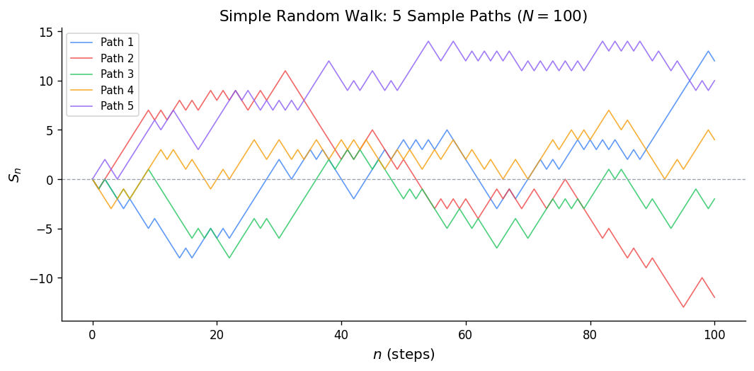
Example: With \(p = 1/2\), what is \(P(S_4 = 0)\)? We need \(u = 2\) up-steps out of 4, so \(P(S_4 = 0) = \binom{4}{2}(1/2)^4 = 6/16 = 3/8\).

\[ u_{2n} = \binom{2n}{n}\frac{1}{4^n} \approx \frac{1}{\sqrt{\pi n}}. \]

This decays to 0 but the sum \(\sum u_{2n}\) diverges (like \(\sum 1/\sqrt{n}\)), which will later confirm that the symmetric walk is recurrent.

Reflection Principle

The key idea: a path from \((0, a)\) to \((n, b)\) with \(a, b > 0\) that touches the axis must cross it at some first time \(\tau\). Reflecting the portion of the path before \(\tau\) about the \(x\)-axis gives a bijection between:

• paths from \((0, a)\) to \((n, b)\) that touch 0, and
• all unrestricted paths from \((0, -a)\) (n, b)).

\[ P(S_1 \neq 0, \ldots, S_n \neq 0, S_n = b \mid S_0 = a) = P(S_n = b \mid S_0 = a) - P(S_n = b \mid S_0 = -a). \]

Example: For the symmetric walk, what is \(P(S_1 > 0, S_2 > 0, S_3 > 0, S_4 > 0, S_4 = 2)\)? By the ballot theorem below, this equals \((2/4) P(S_4 = 2) = (1/2)\binom{4}{3}(1/2)^4 = (1/2)(4/16) = 1/8\).

Ballot Theorem

Setup: Candidate A receives \(a\) votes and candidate B receives \(b\) votes with \(a > b\). In a random ordering of the ballots, what is the probability that A leads B throughout the entire count?

Theorem: This probability is \((a - b)/(a + b)\).

\[ P(S_1 > 0, \ldots, S_n > 0 \mid S_0 = 0, S_n = b) = \frac{b}{n}. \]

Example: \(n = 6\) steps, \(S_6 = 2\) (net). The fraction of strictly-positive paths is \(2/6 = 1/3\). There are \(\binom{6}{4} = 15\) paths total (need 4 up-steps). The number staying positive is \(15 \cdot (1/3) = 5\). One can verify by enumeration.

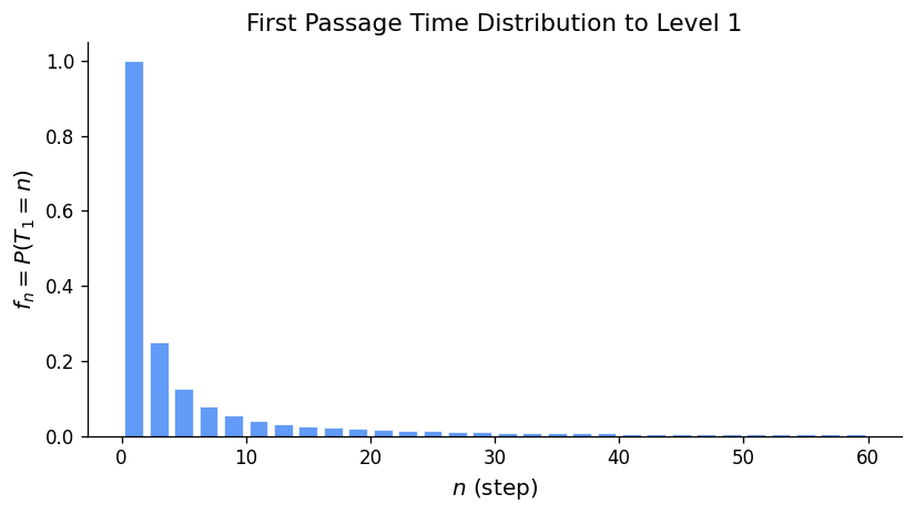
First Passage Times

\[ f_n(b) = P(T_b = n) = \frac{b}{n} P(S_n = b \mid S_0 = 0). \]

Intuition: Among all paths from 0 to \(b\) in \(n\) steps, the fraction that first hit \(b\) at the final step is exactly \(b/n\) — a consequence of a cyclic symmetry (cycle lemma).

\[ f_3(1) = \frac{1}{3} P(S_3 = 1) = \frac{1}{3}\binom{3}{2}(1/2)^3 = \frac{1}{3} \cdot \frac{3}{8} = \frac{1}{8}. \]

Verify directly: the paths from 0 to 1 in 3 steps that hit 1 for the first time at step 3 are those going 0→−1→0→1 (one such path, probability \((1/2)^3 = 1/8\)). ✓

The generating function for first passage to level 1 is \(\Lambda(s) = \frac{1 - \sqrt{1-4pqs^2}}{2qs}\), and by a multiplicative structure argument, the generating function for first passage to level \(b\) is \(F_b(s) = [\Lambda(s)]^b\) — reaching \(b\) requires \(b\) independent first passages of unit height.

Recurrence and Transience of the Random Walk

\[ P(\text{return to 0}) = F(1) = 1 - |p - q|. \]

• Symmetric walk (\(p = q = 1/2\)): \(P(\text{return}) = 1\). The walk is recurrent — it returns to the origin infinitely often.
• Asymmetric walk (\(p \neq 1/2\)): \(P(\text{return}) < 1\). The walk is transient — it drifts off to \(\pm\infty\).

Intuition for recurrence: With \(p = 1/2\), the walk has no drift, so it has “no reason” to escape to infinity. In higher dimensions, the random walk on \(\mathbb{Z}^d\) is recurrent for \(d \leq 2\) (Pólya’s theorem) and transient for \(d \geq 3\) — a striking dimension-dependent phenomenon.

Arcsine Laws

\[ P(L_{2n} = 2k) = u_{2k} \cdot u_{2n-2k} \quad \text{for } k = 0, 1, \ldots, n. \]

Example with \(n = 4\): The possible last-zero times are 0, 2, 4, 6, 8. Using \(u_0 = 1\), \(u_2 = 1/2\), \(u_4 = 3/8\), \(u_6 = 5/16\), \(u_8 = 35/128\):

• \(P(L_8 = 0) = u_0 \cdot u_8 = 35/128\)
• \(P(L_8 = 2) = u_2 \cdot u_6 = (1/2)(5/16) = 5/32 = 20/128\)
• \(P(L_8 = 4) = u_4 \cdot u_4 = (3/8)^2 = 9/64 = 18/128\)
• \(P(L_8 = 6) = u_6 \cdot u_2 = 20/128\)
• \(P(L_8 = 8) = u_8 \cdot u_0 = 35/128\)

Total: \((35 + 20 + 18 + 20 + 35)/128 = 128/128 = 1\). ✓

Notice the probabilities are largest at the extremes (last zero early or late) and smallest in the middle. This is the arcsine shape: the walk tends to spend most of its time on one side of the axis, flipping sides rarely.

In the limit, \(L_{2n}/(2n) \to \text{Arcsine}(0,1)\) distribution with density \(f(x) = \frac{1}{\pi\sqrt{x(1-x)}}\).

\[ P(L_{2n}/(2n) \leq 0.1) + P(L_{2n}/(2n) \geq 0.9) \approx 2 \cdot \frac{2}{\pi}\arcsin(\sqrt{0.1}) \approx 40.5\%. \]

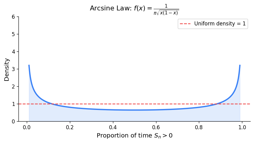
There is roughly a 40% chance the walk spends almost all its time on one side.

---

Generating Functions and Renewal Events

Probability Generating Functions

\[ G(s) = E[s^X] = \sum_{k=0}^\infty p_k s^k, \quad |s| \leq 1. \]\[ E[X] = G'(1), \qquad E[X(X-1)] = G''(1), \qquad \text{Var}(X) = G''(1) + G'(1) - [G'(1)]^2. \]

The PGF of a sum of independent variables is the product: \(G_{X+Y}(s) = G_X(s) G_Y(s)\).

\[ G(s) = \sum_{k=1}^\infty (1-p)^{k-1} p \cdot s^k = \frac{ps}{1-(1-p)s}. \]

Then \(G'(s) = \frac{p}{[1-(1-p)s]^2}\), so \(E[X] = G'(1) = p/p^2 = 1/p\). ✓

\[ G(s) = \sum_{k=0}^\infty \frac{\lambda^k e^{-\lambda}}{k!} s^k = e^{-\lambda} \sum_{k=0}^\infty \frac{(\lambda s)^k}{k!} = e^{\lambda(s-1)}. \]

Then \(G'(s) = \lambda e^{\lambda(s-1)}\), so \(E[X] = G'(1) = \lambda\). \(G''(1) = \lambda^2\), so \(\text{Var}(X) = \lambda^2 + \lambda - \lambda^2 = \lambda\). ✓

Renewal Events

A renewal event is an event that can occur repeatedly over discrete time, with independent and identically distributed inter-occurrence times. Define:

• \(u_n = P(\text{event occurs at time } n)\), with \(u_0 = 1\).
• \(f_n = P(\text{first recurrence at time } n)\) for \(n \geq 1\).

\[ u_n = \sum_{k=1}^n f_k u_{n-k}, \quad n \geq 1. \]

In generating functions: \(U(s) = 1 + F(s)U(s)\), hence \(U(s) = \frac{1}{1-F(s)}\).

Classification:

• Transient: \(F(1) = \sum f_n < 1\). The event occurs only finitely many times.
• Recurrent: \(F(1) = 1\). The event recurs infinitely often with probability 1.
• Positive recurrent: recurrent with \(\mu = \sum n f_n < \infty\) (finite mean inter-renewal time).
• Null recurrent: recurrent with \(\mu = \infty\).
• Periodic with period \(d\): \(f_n = 0\) unless \(d \mid n\).

Example: The symmetric random walk returns to 0. Take \(u_{2k} = P(S_{2k} = 0) = \binom{2k}{k}/4^k\) and \(u_n = 0\) for \(n\) odd. We showed \(\sum_{k=0}^\infty u_{2k} = \infty\) (the sum grows like \(\sum 1/\sqrt{k}\)), so the return event is recurrent. Moreover, the mean return time is \(\mu = \sum_{k=1}^\infty 2k \cdot f_{2k}\). Since \(u_{2k} \approx 1/\sqrt{\pi k} \to 0\), this is null recurrent — the mean return time is infinite, consistent with \(u_{2k} \to 0\).

The Renewal Theorem

Interpretation: In the long run, renewals occur at rate \(1/\mu\) — one per mean inter-renewal time. This is the discrete analogue of the result that a Poisson process with rate \(\lambda = 1/\mu\) has \(E[N(n)]/n \to \lambda\).

Example: Suppose inter-renewal times have \(f_1 = 1/3\), \(f_2 = 2/3\). Then \(\mu = 1 \cdot (1/3) + 2 \cdot (2/3) = 5/3\). The renewal theorem predicts \(u_n \to 3/5 = 0.6\). Let’s verify for small \(n\):

• \(u_0 = 1\)
• \(u_1 = f_1 u_0 = 1/3\)
• \(u_2 = f_1 u_1 + f_2 u_0 = (1/3)(1/3) + (2/3)(1) = 1/9 + 6/9 = 7/9 \approx 0.778\)
• \(u_3 = f_1 u_2 + f_2 u_1 = (1/3)(7/9) + (2/3)(1/3) = 7/27 + 6/27 = 13/27 \approx 0.481\)
• \(u_4 = f_1 u_3 + f_2 u_2 = (1/3)(13/27) + (2/3)(7/9) = 13/81 + 42/81 = 55/81 \approx 0.679\)

The sequence oscillates but converges toward \(0.6\). ✓

---

Branching Processes

Galton-Watson Process

\[ Z_{n+1} = \sum_{i=1}^{Z_n} \xi_i^{(n)}, \quad \xi_i^{(n)} \overset{\text{iid}}{\sim} \{p_k\}. \]\[ E[Z_n] = \mu^n, \qquad \text{Var}(Z_n) = \begin{cases} \sigma^2 \mu^{n-1} \dfrac{\mu^n - 1}{\mu - 1} & \mu \neq 1 \\ n\sigma^2 & \mu = 1 \end{cases} \]

where \(\mu = G'(1)\) (mean offspring) and \(\sigma^2 = G''(1) + G'(1) - [G'(1)]^2\) (offspring variance).

Example — Geometric offspring: Suppose \(P(\text{offspring} = k) = (1/2)^{k+1}\) for \(k = 0, 1, 2, \ldots\) (geometric starting at 0). Then \(G(s) = \sum_{k=0}^\infty (1/2)^{k+1} s^k = \frac{1/2}{1 - s/2} = \frac{1}{2-s}\) and \(\mu = G'(1) = 1/(2-1)^2 = 1\). Since \(\mu = 1\), this is the critical case. The variance of offspring is \(G''(1) + \mu - \mu^2 = \frac{2}{(2-1)^3} + 1 - 1 = 2\). Since \(\sigma^2 = 2 > 0\), extinction is certain.

Extinction Probability

The extinction probability \(\eta = P(\exists n : Z_n = 0)\) satisfies the fixed-point equation \(\eta = G(\eta)\), and is the smallest non-negative root of this equation.

Why \(\eta = G(\eta)\)? Conditioning on the first generation: \(\eta = P(Z_n = 0 \text{ eventually}) = \sum_{k=0}^\infty p_k \eta^k = G(\eta)\). Each of the \(k\) first-generation individuals independently goes extinct with probability \(\eta\).

Classification by \(\mu\):

• Subcritical (\(\mu < 1\)): \(G\) is concave, \(G'(1) < 1\), so the graph of \(G(s)\) on \([0,1]\) lies above the diagonal \(y = s\) everywhere except at \(s = 1\). The only fixed point in \([0,1]\) is \(\eta = 1\). Extinction is certain.
• Critical (\(\mu = 1\)): \(G'(1) = 1\). If \(\sigma^2 > 0\), \(G\) is strictly convex and tangent to \(y = s\) at \(s = 1\), making \(\eta = 1\) the only fixed point in \([0,1]\). Extinction is certain. If \(\sigma^2 = 0\), every individual has exactly one offspring (\(p_1 = 1\)) and the population stays constant forever.
• Supercritical (\(\mu > 1\)): \(G'(1) > 1\), so the line \(y = s\) cuts through the curve \(y = G(s)\) at a second point \(\eta^* \in (0,1)\). Survival with positive probability \(1 - \eta^*\).

Example — Poisson offspring, \(\mu = 1.5\): Let \(Z_1 \sim \text{Poisson}(1.5)\), so \(G(s) = e^{1.5(s-1)}\). Find \(\eta\) solving \(\eta = e^{1.5(\eta - 1)}\). Taking logs: \(\ln \eta = 1.5(\eta - 1)\). Numerically (Newton’s method starting from \(s = 0.5\)): \(\eta \approx 0.583\). So the probability of extinction is about 58.3% and of survival is 41.7%.

Example — Bernoulli offspring: Each individual has 0 children with probability \(1-p\) and 2 children with probability \(p\). Then \(\mu = 2p\).

• \(G(s) = (1-p) + ps^2\).
• Fixed points: \(ps^2 - s + (1-p) = 0\), giving \(s = \frac{1 \pm \sqrt{1 - 4p(1-p)}}{2p} = \frac{1 \pm |1-2p|}{2p}\).
• For \(p > 1/2\) (\(\mu > 1\)): two roots \(\eta = (1-p)/p < 1\) and \(s = 1\). So \(\eta = (1-p)/p\).
• Check: if \(p = 3/4\), then \(\eta = (1/4)/(3/4) = 1/3\). Probability of survival is \(2/3\). ✓

---

Discrete-Time Markov Chains — Definitions and Classification

The Markov Property

\[ P(X_{n+1} = j \mid X_n = i, X_{n-1} = i_{n-1}, \ldots, X_0 = i_0) = P(X_{n+1} = j \mid X_n = i) = p_{ij}. \]

The matrix \(P = (p_{ij})\) is stochastic: \(p_{ij} \geq 0\) and each row sums to 1. For time-homogeneous chains, \(P^n\) gives the \(n\)-step transitions: \(p_{ij}^{(n)} = (P^n)_{ij}\).

Chapman-Kolmogorov: \(p_{ij}^{(m+n)} = \sum_k p_{ik}^{(m)} p_{kj}^{(n)}\), equivalently \(P^{m+n} = P^m P^n\). This is just matrix multiplication — the probability of going from \(i\) to \(j\) in \(m+n\) steps equals the probability of going to some intermediate state \(k\) in \(m\) steps, then from \(k\) to \(j\) in \(n\) more.

Important caution: Satisfying Chapman-Kolmogorov is necessary but not sufficient for the Markov property. There exist processes with the correct marginal pairwise structure but non-Markovian dependencies.

A Worked Example: Two-State Chain

\[ P = \begin{pmatrix} 0.8 & 0.2 \\ 0.4 & 0.6 \end{pmatrix}. \]

This means: given a sunny day, the next day is sunny with probability 0.8; given a rainy day, the next day is sunny with probability 0.4.

\[ p_{00}^{(2)} = (0.8)(0.8) + (0.2)(0.4) = 0.64 + 0.08 = 0.72. \]\[ p_{01}^{(2)} = (0.8)(0.2) + (0.2)(0.6) = 0.16 + 0.12 = 0.28. \]

So starting from a sunny day, after 2 days: sunny with probability 0.72, rainy with probability 0.28.

Classification of States

State \(j\) is accessible from \(i\) (written \(i \to j\)) if \(p_{ij}^{(n)} > 0\) for some \(n\). States \(i, j\) communicate (\(i \leftrightarrow j\)) if \(i \to j\) and \(j \to i\). Communication classes partition \(S\).

Example: Consider the chain on \(\{1,2,3,4,5\}\) with transitions:

• State 1: goes to 2 with prob 1.
• State 2: goes to 1 with prob \(1/2\), goes to 3 with prob \(1/2\).
• State 3: goes to 4 with prob 1.
• State 4: goes to 3 with prob \(1/2\), stays at 4 with prob \(1/2\).
• State 5: goes to 5 with prob 1 (absorbing).

Communication classes: \(\{1,2\}\) (communicate), \(\{3,4\}\) (communicate), \(\{5\}\) (alone). Class \(\{1,2\}\) is open (can escape to 3). Class \(\{3,4\}\) is closed. Class \(\{5\}\) is closed (absorbing).

Recurrence and Transience

Let \(f_{jj} = P(T_j < \infty \mid X_0 = j)\) be the probability of ever returning to \(j\).

Proof sketch: The number of visits to \(j\) is \(V_j = \sum_{n=0}^\infty \mathbf{1}_{X_n = j}\). Each visit produces another visit with probability \(f_{jj}\), so \(V_j\) is geometric-like: \(E[V_j \mid X_0 = j] = 1/(1-f_{jj})\) if transient, and \(\infty\) if recurrent. Since \(E[V_j] = \sum p_{jj}^{(n)}\), the result follows.

Recurrence is a class property: If \(i \leftrightarrow j\), there exist \(m, n\) with \(p_{ij}^{(m)} > 0\) and \(p_{ji}^{(n)} > 0\). Since \(p_{jj}^{(m+k+n)} \geq p_{ji}^{(n)} p_{ii}^{(k)} p_{ij}^{(m)}\), summing over \(k\): if \(\sum p_{ii}^{(k)} = \infty\) then \(\sum p_{jj}^{(k)} = \infty\).

Example — Simple random walk: \(p_{00}^{(n)} = u_n \approx 1/\sqrt{\pi n}\) for even \(n\), zero for odd \(n\). Since \(\sum_{k=1}^\infty 1/\sqrt{k} = \infty\), state 0 is recurrent. ✓

Example — Asymmetric random walk (\(p = 0.6\), \(q = 0.4\)): The generating function \(U(s) = (1 - 4pqs^2)^{-1/2} = (1 - 0.96s^2)^{-1/2}\) converges at \(s = 1\) since \(U(1) = (1-0.96)^{-1/2} = (0.04)^{-1/2} = 5 < \infty\). So the walk is transient. The probability of ever returning to 0 is \(f_{00} = 1 - 1/U(1) = 1 - 1/5 = 0.8\). Wait — this gives \(f_{00} = F(1) = 1 - |p-q| = 1 - 0.2 = 0.8\). Then \(\sum p_{00}^{(n)} = 1/(1-0.8) = 5\). ✓

Period

The period \(d(i) = \gcd\{n \geq 1 : p_{ii}^{(n)} > 0\}\). State \(i\) is aperiodic if \(d(i) = 1\).

Example: Simple random walk on \(\mathbb{Z}\). From state 0, returns are only possible at even times: \(p_{00}^{(2k+1)} = 0\). So \(d(0) = 2\). The walk is periodic with period 2.

Example: The weather chain above — from state 0, \(p_{00}^{(1)} = 0.8 > 0\), so \(d(0) = 1\). The chain is aperiodic.

Practical tip: A chain is aperiodic if any state has a self-loop (\(p_{ii} > 0\)), since then \(\gcd\{1, \ldots\} = 1\).

Positive and Null Recurrence

For a recurrent state \(j\), let \(\mu_j = E[T_j \mid X_0 = j]\) be the mean return time. State \(j\) is positive recurrent if \(\mu_j < \infty\), null recurrent if \(\mu_j = \infty\).

Example — Positive recurrent (finite chain): The two-state weather chain is irreducible on a finite state space, so all states are positive recurrent. We can compute \(\mu_0 = 1/\pi_0\) once we find the stationary distribution.

Example — Null recurrent: The simple symmetric random walk on \(\mathbb{Z}\) is recurrent. The mean return time to 0 is infinite — you will return with probability 1, but on average it takes infinitely long. This is why \(u_{2n} \to 0\) (consistent with \(\mu_0 = \infty\), so \(\pi_0 = 1/\mu_0 = 0\)).

Finite state space: Any irreducible chain on a finite state space has all states positive recurrent. There are no null recurrent states in finite chains.

Gambler’s Ruin

The classic gambler’s ruin problem illustrates recurrence, first passage, and absorption in one example.

Setup: A gambler starts with $\(k\) and plays repeatedly, winning $1 with probability \(p\) and losing $1 with probability \(q = 1-p\). The game ends when wealth reaches 0 (ruin) or \(N\) (goal). Let \(r_k = P(\text{ruin} \mid \text{start at } k)\).

\[ r_k = p \cdot r_{k+1} + q \cdot r_k + \text{...wait, no:} \quad r_k = p \cdot r_{k+1} + q \cdot r_{k-1}, \]\[ r_k = \frac{(q/p)^k - (q/p)^N}{1 - (q/p)^N}. \]

For \(p = q = 1/2\): \(r_k = 1 - k/N\) (linear). For \(p > q\): \((q/p)^k < 1\), so as \(N \to \infty\), \(r_k \to (q/p)^k\). There is positive probability of never being ruined.

\[ r_5 = \frac{(2/3)^5 - (2/3)^{10}}{1 - (2/3)^{10}} = \frac{0.1317 - 0.01734}{1 - 0.01734} \approx \frac{0.1143}{0.9827} \approx 0.116. \]

A 11.6% chance of ruin starting at $5 with a $10 goal, even with a favourable 60% win probability.

---

Stationary Distributions and Limit Theorems

Stationary Distributions

A distribution \(\pi\) is stationary if \(\pi P = \pi\), i.e., \(\pi_j = \sum_i \pi_i p_{ij}\) for all \(j\), with \(\pi_j \geq 0\) and \(\sum_j \pi_j = 1\). If the chain starts in \(\pi\), it stays in \(\pi\) forever.

How to find \(\pi\): Solve the linear system \(\pi P = \pi\) with normalization \(\sum \pi_j = 1\). In matrix form, \(\pi(P - I) = \mathbf{0}\) — replace one equation with \(\sum \pi_j = 1\).

\[ P = \begin{pmatrix} 0.8 & 0.2 \\ 0.4 & 0.6 \end{pmatrix}. \]

Balance equations: \(\pi_0 = 0.8\pi_0 + 0.4\pi_1\) and \(\pi_1 = 0.2\pi_0 + 0.6\pi_1\). From the first: \(0.2\pi_0 = 0.4\pi_1\), so \(\pi_0 = 2\pi_1\). With \(\pi_0 + \pi_1 = 1\): \(\pi_0 = 2/3\), \(\pi_1 = 1/3\). In the long run, 2/3 of days are sunny.

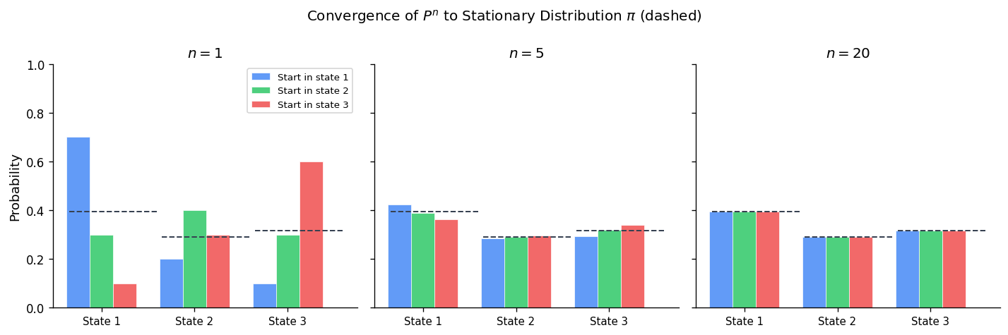
\[ P = \begin{pmatrix} 0 & 1/2 & 1/2 \\ 1/3 & 1/3 & 1/3 \\ 1/2 & 1/2 & 0 \end{pmatrix}. \]

Solve \(\pi P = \pi\):

• \(\pi_A = \pi_B/3 + \pi_C/2\)
• \(\pi_B = \pi_A/2 + \pi_B/3 + \pi_C/2\)
• \(\pi_C = \pi_A/2 + \pi_B/3\)

From symmetry between \(A\) and \(C\) (the matrix is symmetric under swapping \(A \leftrightarrow C\)): \(\pi_A = \pi_C\). Substituting into the first equation: \(\pi_A = \pi_B/3 + \pi_A/2\), so \(\pi_A/2 = \pi_B/3\), giving \(\pi_B = 3\pi_A/2\). Normalization: \(\pi_A + 3\pi_A/2 + \pi_A = 1 \Rightarrow 7\pi_A/2 = 1 \Rightarrow \pi_A = 2/7\). So \(\pi = (2/7, 3/7, 2/7)\).

Key implication: \(\pi_j = 1/\mu_j\) gives a beautiful interpretation — the stationary probability of being in state \(j\) is the reciprocal of the mean return time. States visited more often (smaller \(\mu_j\)) have higher stationary probability.

Example — Verifying \(\pi_j = 1/\mu_j\) for the weather chain: We found \(\pi_0 = 2/3\). So the mean return time to “Sunny” is \(\mu_0 = 1/\pi_0 = 3/2\). Let’s verify directly: starting from state 0 (Sunny), with probability 0.8 we return immediately in 1 step; with probability 0.2 we go to state 1, from which we return to 0 with probability 0.4 per step (geometric waiting time with mean \(1/0.4 = 2.5\) more steps). So \(\mu_0 = 1 \cdot 0.8 + (1 + 1/0.4) \cdot 0.2 = 0.8 + (3.5)(0.2) = 0.8 + 0.7 = 1.5\). ✓

First-Step Analysis for Mean Hitting Times

To compute mean hitting times, write a system of equations by conditioning on the first step.

Example — Three states \(\{0,1,2\}\): Transitions: \(p_{01} = p_{10} = p_{12} = p_{21} = 1/2\) and \(p_{02} = p_{20} = 1/2\). Find \(\mu_0 = E[T_0 \mid X_0 = 0]\).

Let \(h_i = E[T_0 \mid X_0 = i]\) for \(i \neq 0\). First-step analysis: \(h_1 = 1 + \frac{1}{2} h_0 + \frac{1}{2} h_2\) but \(h_0 = 0\) (already at 0, but we want the return time from 0, not the hitting time from 0). More carefully: \(\mu_0 = 1 + \frac{1}{2} h_1^{(0)} + \frac{1}{2} h_2^{(0)}\) where \(h_i^{(0)}\) is the expected time to reach 0 from \(i\). The symmetry of the chain gives \(h_1^{(0)} = h_2^{(0)}\) (not obvious here — better to just solve the system).

Limit Theorem

Proof via coupling: Construct two independent chains: \(\{X_n\}\) starting at \(i\) and \(\{Y_n\}\) started with \(Y_0 \sim \pi\). Since \(Y_n \sim \pi\) for all \(n\), the coupling time \(\tau = \min\{n : X_n = Y_n\}\) is almost surely finite (irreducibility + aperiodicity guarantee the chains meet). After meeting, they run together. Then \(|p_{ij}^{(n)} - \pi_j| \leq P(\tau > n) \to 0\).

Example — Two-state chain, convergence rate: The eigenvalues of the weather chain \(P\) are \(\lambda_1 = 1\) and \(\lambda_2 = 0.8 - 0.4 = 0.4\) (the second eigenvalue equals the trace minus 1 divided appropriately). The rate of convergence is \(|\lambda_2|^n = 0.4^n\).

\[ P^n = \begin{pmatrix} 2/3 & 1/3 \\ 2/3 & 1/3 \end{pmatrix} + 0.4^n \begin{pmatrix} 1/3 & -1/3 \\ -2/3 & 2/3 \end{pmatrix}. \]

For \(n = 5\): \(0.4^5 = 0.01024\), so the deviation from stationarity is about 1%. After 10 steps: \(0.4^{10} \approx 0.0001\) — essentially converged.

Periodic chains: For a periodic chain with period \(d\), the limit \(p_{ij}^{(n)}\) does not exist, but Cesàro averages converge: \(\frac{1}{n}\sum_{k=0}^{n-1} p_{ij}^{(k)} \to \pi_j\).

---

Reversibility and Detailed Balance

Time Reversal

\[ q_{ij} = \frac{\pi_j p_{ji}}{\pi_i}. \]

Verification that \(Q\) is stochastic: \(\sum_j q_{ij} = \sum_j \frac{\pi_j p_{ji}}{\pi_i} = \frac{1}{\pi_i}\sum_j \pi_j p_{ji} = \frac{\pi_i}{\pi_i} = 1\). ✓

Detailed Balance and Reversibility

\[ \pi_i p_{ij} = \pi_j p_{ji} \quad \text{for all } i,j. \]

These are the detailed balance equations. They say the probability flux from \(i\) to \(j\) equals the flux from \(j\) to \(i\) — a detailed microscopic balance, stronger than the global balance \(\pi_j = \sum_i \pi_i p_{ij}\).

Proof: Sum detailed balance over \(i\): \(\sum_i \pi_i p_{ij} = \sum_i \pi_j p_{ji} = \pi_j\). So \((\pi P)_j = \pi_j\). \(\square\)

When to use detailed balance: Detailed balance is easier to verify than \(\pi P = \pi\) directly — there are \(|S|^2\) equations instead of \(|S|\), but they are all of the simple form “product of two terms equals product of two terms.”

Birth-Death Chains and Detailed Balance

\[ \pi_n = \pi_0 \cdot \frac{\lambda_0 \lambda_1 \cdots \lambda_{n-1}}{\mu_1 \mu_2 \cdots \mu_n}. \]

All birth-death chains satisfy detailed balance and are therefore reversible.

Example — Random walk on \(\{0,1,2,3\}\) with reflecting boundaries. \(p_{01} = 1\), \(p_{32} = 1\), and for interior: \(p_{i,i+1} = p_{i,i-1} = 1/2\). Detailed balance: \(\pi_i \cdot (1/2) = \pi_{i+1} \cdot (1/2)\) for interior transitions, so \(\pi_0 = \pi_1 = \pi_2 = \pi_3\). Normalizing: \(\pi_i = 1/4\). The uniform distribution is stationary.

Example — Non-reversible chain: Cyclic chain on \(\{0, 1, 2\}\) with \(p_{01} = p_{12} = p_{20} = 1\). Check detailed balance: \(\pi_0 p_{01} = \pi_1 p_{10}\) requires \(\pi_0 \cdot 1 = \pi_1 \cdot 0 = 0\), impossible. Not reversible. The stationary distribution is \(\pi = (1/3, 1/3, 1/3)\), but detailed balance fails.

Using Detailed Balance to Find \(\pi\): A Full Example

\[ p_{01} = 0.3, \; p_{10} = 0.5, \; p_{12} = 0.5, \; p_{21} = 0.4, \; p_{23} = 0.6, \; p_{32} = 1. \]

(birth-death structure). Detailed balance:

• \(\pi_0 \cdot 0.3 = \pi_1 \cdot 0.5 \Rightarrow \pi_1 = 0.6\pi_0\)
• \(\pi_1 \cdot 0.5 = \pi_2 \cdot 0.4 \Rightarrow \pi_2 = (0.5/0.4)\pi_1 = 1.25 \cdot 0.6\pi_0 = 0.75\pi_0\)
• \(\pi_2 \cdot 0.6 = \pi_3 \cdot 1 \Rightarrow \pi_3 = 0.6 \cdot 0.75\pi_0 = 0.45\pi_0\)

Normalization: \(\pi_0(1 + 0.6 + 0.75 + 0.45) = 1 \Rightarrow \pi_0 = 1/2.8 \approx 0.357\).

---

Discrete Phase-Type Distributions

Definition and Setup

\[ P = \begin{pmatrix} Q & \tilde{q}\mathbf{e}' \\ \mathbf{0} & 1 \end{pmatrix} \]

where \(Q\) is \(m \times m\) sub-stochastic (transitions among transient states), \(\tilde{q} = \mathbf{1} - Q\mathbf{1}\) is the vector of one-step absorption probabilities. The absorption time \(T = \min\{n \geq 0 : X_n \text{ absorbing}\}\) with initial distribution \(\alpha_0\) over transient states satisfies \(T \sim \mathrm{DPH}_m(\alpha_0, Q)\).

PMF, CDF, and Mean

\[ P(T = k) = \alpha_0' Q^{k-1} \tilde{q}, \quad k = 1, 2, \ldots \]\[ P(T > k) = \alpha_0' Q^k \mathbf{1}, \quad F_T(k) = 1 - \alpha_0' Q^k \mathbf{1} \]\[ E[T] = \alpha_0'(I-Q)^{-1}\mathbf{1} \]

Why the mean formula works: \(E[T] = \sum_{k=1}^\infty P(T \geq k) = \sum_{k=1}^\infty P(T > k-1) = \sum_{k=0}^\infty \alpha_0' Q^k \mathbf{1} = \alpha_0'(I-Q)^{-1}\mathbf{1}\), using the matrix geometric series \(\sum_{k=0}^\infty Q^k = (I-Q)^{-1}\) which converges because all eigenvalues of \(Q\) satisfy \(|\lambda| < 1\).

Detailed Worked Example

Setup: A system has two transient phases. From phase 1, with probability 0.3 the system is completed (absorbed) and with probability 0.7 it moves to phase 2. From phase 2, with probability 0.5 the system is completed and with probability 0.5 it returns to phase 1. Let \(T\) be the total time until completion, starting always in phase 1.

\[ Q = \begin{pmatrix} 0 & 0.7 \\ 0.5 & 0 \end{pmatrix}, \quad \tilde{q} = \begin{pmatrix} 0.3 \\ 0.5 \end{pmatrix}. \]

PMF:

• \(P(T = 1) = \alpha_0' Q^0 \tilde{q} = (1,0)(0.3, 0.5)' = 0.3\). (Absorbed from phase 1 directly.)
• \(P(T = 2) = \alpha_0' Q \tilde{q} = (1,0)\begin{pmatrix}0&0.7\\0.5&0\end{pmatrix}\begin{pmatrix}0.3\\0.5\end{pmatrix}\). First compute \(Q\tilde{q} = (0 \cdot 0.3 + 0.7 \cdot 0.5, \; 0.5 \cdot 0.3 + 0 \cdot 0.5)' = (0.35, 0.15)'\). Then \(P(T=2) = (1,0)(0.35, 0.15)' = 0.35\).
• \(P(T = 3) = \alpha_0' Q^2 \tilde{q}\). Compute \(Q^2 = \begin{pmatrix}0.35 & 0 \\ 0 & 0.35\end{pmatrix}\). Then \(Q^2\tilde{q} = (0.35 \cdot 0.3, 0.35 \cdot 0.5)' = (0.105, 0.175)'\). So \(P(T=3) = 0.105\).

Check: \(P(T=1) + P(T=2) + P(T=3) + \cdots = 0.3 + 0.35 + \cdots\). We have \(P(T > 2) = \alpha_0' Q^2 \mathbf{1} = (1,0)(Q^2)\mathbf{1}\). Since \(Q^2 = 0.35 I\), \(P(T > 2) = 0.35\). Then \(P(T=1)+P(T=2) = 1 - 0.35 = 0.65\). ✓ (\(0.3 + 0.35 = 0.65\).)

\[ I - Q = \begin{pmatrix}1 & -0.7 \\ -0.5 & 1\end{pmatrix}, \quad (I-Q)^{-1} = \frac{1}{1 - 0.35}\begin{pmatrix}1 & 0.7 \\ 0.5 & 1\end{pmatrix} = \frac{1}{0.65}\begin{pmatrix}1 & 0.7 \\ 0.5 & 1\end{pmatrix}. \]\[ E[T] = \alpha_0'(I-Q)^{-1}\mathbf{1} = (1,0)\frac{1}{0.65}\begin{pmatrix}1 & 0.7\\ 0.5 & 1\end{pmatrix}\begin{pmatrix}1\\1\end{pmatrix} = \frac{1}{0.65}(1,0)\begin{pmatrix}1.7\\1.5\end{pmatrix} = \frac{1.7}{0.65} \approx 2.615. \]

Geometric Distribution as DPH

\(\text{Geometric}(p)\) with \(P(T = k) = (1-p)^{k-1}p\) for \(k \geq 1\) corresponds to \(\mathrm{DPH}_1(1, 1-p)\): one transient state, \(Q = (1-p)\), \(\alpha_0 = 1\), \(\tilde{q} = p\).

Check: \(P(T=k) = 1 \cdot (1-p)^{k-1} \cdot p\). ✓ Mean: \(E[T] = 1 \cdot (1-(1-p))^{-1} \cdot 1 = 1/p\). ✓

Closure Under Independent Sum

\[ \gamma = (\alpha, \mathbf{0}), \qquad C = \begin{pmatrix} Q & \tilde{q}\beta' \\ \mathbf{0} & R \end{pmatrix}. \]

Interpretation: The combined chain first runs through the \(X\)-phases (governed by \(Q\)). When it would be absorbed (with probability \(\tilde{q}_i\) from state \(i\)), instead of absorbing it jumps to start the \(Y\)-chain in state \(j\) with probability \(\beta_j\). It then runs through the \(Y\)-phases (governed by \(R\)) until true absorption.

\[ C = \begin{pmatrix} 1-p & p \\ 0 & 1-q \end{pmatrix}, \quad \gamma = (1,0). \]

This is the negative hypergeometric / convolution of two geometrics. Note that if \(p = q\), then \(Z\) has a negative binomial distribution.

---

The Poisson Process

Definition and Derivation

The Poisson process \(\{N(t)\}_{t \geq 0}\) counts events occurring in continuous time. The three defining axioms are:

1. Ordinarity (individuality): \(P(N(t+h) - N(t) \geq 2) = o(h)\) — at most one event per infinitesimal interval.
2. Stationarity and homogeneity: \(P(N(t+h) - N(t) = 1) = \lambda h + o(h)\) — the rate \(\lambda\) is constant.
3. Independence of increments: disjoint intervals are independent.

\[ p_k(t+h) = p_k(t)(1-\lambda h) + p_{k-1}(t)\lambda h + o(h). \]

Dividing by \(h\) and taking \(h \to 0\): \(p_k'(t) = -\lambda p_k(t) + \lambda p_{k-1}(t)\). With \(p_0(0) = 1\) and \(p_k(0) = 0\) for \(k \geq 1\), solving recursively gives \(p_k(t) = e^{-\lambda t}(\lambda t)^k/k!\).

Inter-Arrival Times

The waiting times between events \(X_k = S_k - S_{k-1}\) are iid Exponential(\(\lambda\)). Why? By the independence and stationarity of increments, \(P(X_1 > t) = P(N(t) = 0) = e^{-\lambda t}\). Given that the first event has not occurred by time \(s\), the waiting time from \(s\) onward has the same distribution as the original wait — the memoryless property.

Example: A call center receives calls at rate \(\lambda = 5\) per hour. What is the probability of waiting more than 20 minutes for the first call? \(P(X_1 > 1/3) = e^{-5/3} \approx 0.189\). Expected wait: \(E[X_1] = 1/5\) hour = 12 minutes.

Conditional Distribution of Arrival Times (Order Statistics Property)

Given \(N(t) = n\), the \(n\) arrival times \(S_1 < S_2 < \cdots < S_n\) have the same joint distribution as the order statistics of \(n\) iid Uniform\((0,t)\) random variables. Equivalently, the unordered arrival times are uniformly and independently scattered in \([0,t]\).

Example: Bus arrivals follow a Poisson process with rate 3 per hour. Given that 4 buses arrived in a 2-hour window, what is the probability that all 4 arrived in the first hour? This equals the probability that all 4 uniform\((0,2)\) points fall in \([0,1]\): \((1/2)^4 = 1/16\).

Example: Conditional on \(N(1) = 3\), the expected time of the first arrival is \(E[S_{(1)}] = E[\min(U_1, U_2, U_3)]\) where \(U_i \sim \text{Uniform}(0,1)\). Since the minimum of \(n\) uniforms has mean \(1/(n+1)\): \(E[S_1 \mid N(1) = 3] = 1/4\).

Superposition and Thinning

Superposition: If \(N_1(t) \sim \text{Poisson}(\lambda_1 t)\) and \(N_2(t) \sim \text{Poisson}(\lambda_2 t)\) are independent, then \(N_1(t) + N_2(t) \sim \text{Poisson}((\lambda_1+\lambda_2)t)\).

Proof via MGF: \(E[e^{s(N_1+N_2)}] = e^{\lambda_1 t(e^s-1)} e^{\lambda_2 t(e^s-1)} = e^{(\lambda_1+\lambda_2)t(e^s-1)}\). ✓

Thinning: If each arrival is independently type 1 with probability \(p\) or type 2 with probability \(1-p\), then \(N_1(t) \sim \text{Poisson}(\lambda p t)\) and \(N_2(t) \sim \text{Poisson}(\lambda(1-p)t)\) are independent.

Example: Emails arrive at rate 20 per hour. Spam emails are 30% of all arrivals. Then spam arrives at rate 6/hr and legitimate emails at rate 14/hr, and the two processes are independent Poisson.

Examples with Superposition and Thinning

Example: Customers arrive at a bank at rate 10/hour. Each customer is either a retail customer (prob 0.6) or a business customer (prob 0.4). What is the probability that the 5th business customer arrives before the 3rd retail customer?

Let \(N_R(t) \sim \text{Poisson}(6t)\) (retail) and \(N_B(t) \sim \text{Poisson}(4t)\) (business), independent. Let \(S_5^B\) be the time of the 5th business arrival and \(S_3^R\) the 3rd retail arrival. Since \(S_5^B \sim \text{Gamma}(5, 4)\) and \(S_3^R \sim \text{Gamma}(3, 6)\), computing \(P(S_5^B < S_3^R)\) requires integration (or simulation). Alternatively, note that each individual arrival is business with probability \(4/10 = 0.4\). We need the 5th business to come before the 3rd retail — equivalently, among the first 6 arrivals, at least 5 are business. By the binomial: \(P = P(\text{Bin}(6, 0.4) \geq 5) = \binom{6}{5}0.4^5 0.6 + \binom{6}{6}0.4^6 = 6(0.01024)(0.6) + 0.004096 = 0.03686 + 0.004096 \approx 0.041\).

---

Continuous-Time Markov Chains — Generator and Equations

Definition and Setup

A CTMC \(\{X(t)\}_{t \geq 0}\) on countable state space \(S\) satisfies the Markov property in continuous time. The transition functions \(P_{ij}(t) = P(X(t+s) = j \mid X(s) = i)\) form a semi-group: \(P(0) = I\), \(P(s+t) = P(s)P(t)\) (Chapman-Kolmogorov).

Infinitesimal Generator

\[ g_{ij} = \lim_{h \downarrow 0} \frac{P_{ij}(h) - \delta_{ij}}{h}. \]

For \(i \neq j\): \(g_{ij} \geq 0\) is the transition rate from \(i\) to \(j\). For \(i = j\): \(g_{ii} = -v_i \leq 0\) where \(v_i = \sum_{j \neq i} g_{ij}\) is the total exit rate from state \(i\). Row sums equal zero: \(g_{ii} + \sum_{j \neq i} g_{ij} = 0\).

\[ P_{ii}(h) = 1 - v_i h + o(h), \qquad P_{ij}(h) = g_{ij} h + o(h), \; i \neq j. \]

Sojourn Times and Embedded Chain

Sojourn time in state \(i\): The time spent in state \(i\) before jumping is \(\text{Exp}(v_i)\). This follows from the memoryless property and the small-\(h\) approximation: the probability of still being in state \(i\) at time \(h\) given just arrived is \(e^{-v_i h}\).

\[ \hat{p}_{ij} = \frac{g_{ij}}{v_i}. \]

The sequence of visited states forms a DTMC with transition matrix \(\hat{P}\) (no self-loops: \(\hat{p}_{ii} = 0\)).

\[ G = \begin{pmatrix} -\alpha & \alpha \\ \beta & -\beta \end{pmatrix}. \]

State 0 exits at rate \(\alpha\) (always to state 1) and state 1 exits at rate \(\beta\) (always to state 0). The chain alternates between 0 and 1, spending Exp(\(\alpha\)) time in state 0 and Exp(\(\beta\)) time in state 1.

Kolmogorov Equations and Matrix Exponential

\[ P(t) = e^{tG} = \sum_{n=0}^\infty \frac{(tG)^n}{n!}. \]\[ P(t) = \frac{1}{\alpha+\beta}\begin{pmatrix}\beta & \alpha \\ \beta & \alpha\end{pmatrix} + \frac{e^{-(\alpha+\beta)t}}{\alpha+\beta}\begin{pmatrix}\alpha & -\alpha \\ -\beta & \beta\end{pmatrix}. \]\[ P_{00}(t) = \frac{\beta}{\alpha+\beta} + \frac{\alpha}{\alpha+\beta}e^{-(\alpha+\beta)t}, \quad P_{01}(t) = \frac{\alpha}{\alpha+\beta} - \frac{\alpha}{\alpha+\beta}e^{-(\alpha+\beta)t}. \]

Interpretation: Starting from state 0, the probability of being in state 0 at time \(t\) decays exponentially from 1 toward the stationary probability \(\beta/(\alpha+\beta)\).

Numerical example: \(\alpha = 2\) (leave state 0 at rate 2), \(\beta = 3\) (leave state 1 at rate 3). Stationary: \(\pi_0 = 3/5\), \(\pi_1 = 2/5\). At \(t = 1\): \(P_{00}(1) = 3/5 + (2/5)e^{-5} \approx 0.6 + 0.00539 \approx 0.605\). Already close to stationary!

Uniformization

\[ \hat{P}_{ij} = \frac{g_{ij}}{\Lambda} + \delta_{ij}\left(1 - \frac{v_i}{\Lambda}\right). \]\[ P_{ij}(t) = \sum_{n=0}^\infty \frac{(\Lambda t)^n e^{-\Lambda t}}{n!} \hat{p}_{ij}^{(n)}. \]\[ \hat{P} = \begin{pmatrix} 1-2/3 & 2/3 \\ 1 & 0 \end{pmatrix} = \begin{pmatrix} 1/3 & 2/3 \\ 1 & 0 \end{pmatrix}. \]

Then \(P_{00}(t) = \sum_{n=0}^\infty \frac{(3t)^n e^{-3t}}{n!} \hat{p}_{00}^{(n)}\). This is useful when computing \(P(t)\) by hand is complex but matrix powers of \(\hat{P}\) can be computed iteratively.

---

CTMC — Classification and Stationary Distributions

Classification of States

Classification in CTMCs mirrors DTMCs, with one major simplification: there is no periodicity. Because sojourn times are continuous, the chain can return to any state at any positive time, eliminating the integer-period structure of DTMCs.

Accessibility: \(i \to j\) in the CTMC iff \(i \to j\) in the embedded DTMC (this equivalence holds because \(P_{ij}(t) > 0\) iff there is a positive-probability path of jumps from \(i\) to \(j\)).

Recurrence: Defined as in DTMCs. For the embedded chain, the classification via \(\sum_n \hat{p}_{jj}^{(n)}\) applies. But note:

Key subtlety — positive vs. null recurrence in CTMC vs. embedded DTMC: A state can be positive recurrent in the embedded DTMC (finite expected number of jumps to return) but null recurrent in the CTMC (infinite expected time to return). This happens when the mean sojourn times grow with each visit, inflating the total expected return time.

The mean CTMC return time: \(E[R_{ii}] = \mu_i^{\text{embedded}} / v_i\) — the mean number of embedded steps to return times the mean sojourn time per step. If \(1/v_i \to \infty\) along returning paths, the CTMC can be null recurrent even with a positive recurrent embedded chain.

Stationary Distribution

\[ \pi_j v_j = \sum_{i \neq j} \pi_i g_{ij} \quad \text{(rate out of } j\text{ = rate into }j\text{)}. \]\[ \pi_j = \frac{\psi_j / v_j}{\sum_k \psi_k / v_k}. \]

The CTMC weights each state by the mean sojourn time \(1/v_j\) — states with slow exit rates get extra probability because the chain lingers there longer.

\[ -\alpha \pi_0 + \beta \pi_1 = 0 \Rightarrow \pi_0 = \frac{\beta}{\alpha+\beta}, \quad \pi_1 = \frac{\alpha}{\alpha+\beta}. \]

With \(\alpha = 2\), \(\beta = 3\): \(\pi_0 = 3/5\), \(\pi_1 = 2/5\). Interpretation: the chain spends 60% of its time in state 0 and 40% in state 1 — weighted by the mean sojourn times \(1/\alpha = 0.5\) and \(1/\beta = 1/3\) (state 0 has longer sojourns, consistent with its higher stationary probability).

Limiting theorem:

There is no need to assume aperiodicity (unlike DTMCs) because CTMCs are automatically “aperiodic” in the continuous-time sense.

PASTA Property

PASTA (Poisson Arrivals See Time Averages): If customers arrive according to a Poisson process and the system evolves independently of arrival times, then an arriving customer sees the time-stationary distribution of the system state.

\[ \lim_{n\to\infty} P(X(S_n^-) = j) = \pi_j \]

where \(S_n\) is the \(n\)-th arrival epoch and \(X(S_n^-)\) is the system state just before the arrival.

Why this matters: For an M/M/1 queue, PASTA implies the fraction of arriving customers who find \(k\) customers in the system equals \(\pi_k = (1-\rho)\rho^k\) — which also equals the time-average probability of \(k\) customers. This identity simplifies performance analysis enormously.

Why PASTA fails for non-Poisson arrivals: A deterministic arrival process (e.g., one customer every 10 seconds) can be synchronized with the system dynamics, causing arrivals to systematically see atypical states.

Example — M/M/1 application: With \(\lambda = 4\) arrivals/hr and \(\mu = 6\) service rate, \(\rho = 4/6 = 2/3\). By PASTA:

• Fraction of arrivals finding an empty system: \(\pi_0 = 1/3\).
• Fraction finding 2 or more: \(\sum_{k=2}^\infty (1-2/3)(2/3)^k = (2/3)^2 = 4/9 \approx 44\%\).

---

Birth and Death Processes

Setup

\[ g_{i,i+1} = \lambda_i, \quad g_{i,i-1} = \mu_i \; (\mu_0 = 0), \quad g_{ii} = -(\lambda_i + \mu_i). \]

Stationary Distribution via Detailed Balance

\[ \pi_n = \pi_0 \cdot \frac{\lambda_0 \lambda_1 \cdots \lambda_{n-1}}{\mu_1 \mu_2 \cdots \mu_n} \equiv \pi_0 \rho_n, \quad \pi_0 = \frac{1}{\sum_{n=0}^\infty \rho_n}. \]

The chain is positive recurrent (stationary distribution exists) iff \(\sum_{n=0}^\infty \rho_n < \infty\).

Special Cases

Poisson process: \(\lambda_n = \lambda\), \(\mu_n = 0\). The chain is a pure birth process — \(N(t)\) counts arrivals. Since \(\mu_n = 0\), the chain is transient (never goes back down). No stationary distribution.

Yule process: \(\lambda_n = n\lambda\), \(\mu_n = 0\). Each individual reproduces at rate \(\lambda\), so the birth rate is proportional to the current population. Starting from \(X(0) = 1\), \(P(X(t) = k) = e^{-\lambda t}(1-e^{-\lambda t})^{k-1}\) for \(k \geq 1\) (geometric). The mean population is \(E[X(t)] = e^{\lambda t}\) — exponential growth.

\[ \pi_n = \frac{(\nu/\mu)^n e^{-\nu/\mu}}{n!}. \]

Why? Check: \(\rho_n = \nu^n / (\mu^n n!) \cdot \nu^0 = (\nu/\mu)^n/n!\) (a Poisson numerator), and \(\sum \rho_n = e^{\nu/\mu}\), so \(\pi_0 = e^{-\nu/\mu}\). ✓

Linear growth (simple birth-death): \(\lambda_n = n\lambda\), \(\mu_n = n\mu\). The chain can go extinct (reach 0) which is absorbing. For \(\lambda > \mu\): the process tends to grow with extinction probability \((\mu/\lambda)^{X_0}\). For \(\lambda \leq \mu\): extinction is certain. This mirrors the branching process.

Full Example: M/M/1/∞ as Birth-Death

The M/M/1 queue has \(\lambda_n = \lambda\) and \(\mu_n = \mu\) for \(n \geq 1\), \(\mu_0 = 0\). The traffic intensity is \(\rho = \lambda/\mu\).

\[ \pi_n = (1-\rho)\rho^n. \]

Performance measures:

• Mean queue length: \(E[N] = \sum_{n=0}^\infty n\pi_n = \rho/(1-\rho)\).

  Derivation: \(E[N] = (1-\rho)\sum_{n=0}^\infty n\rho^n = (1-\rho)\frac{\rho}{(1-\rho)^2} = \frac{\rho}{1-\rho}\).

• Server utilization: \(P(N \geq 1) = \rho\). Makes sense: rate in = rate out in steady state, so \(\lambda = \mu \cdot P(\text{server busy})\), giving \(P(\text{busy}) = \rho\).

• \[ E[W] = \frac{E[N]}{\lambda} = \frac{\rho}{\lambda(1-\rho)} = \frac{1}{\mu - \lambda}. \]

• Mean time in queue (excluding service): \(E[W_q] = E[W] - 1/\mu = \rho/(\mu-\lambda)\).

Numerical example: \(\lambda = 8\) customers/hr, \(\mu = 10\)/hr. Then \(\rho = 0.8\).

• \(\pi_0 = 0.2\) (20% of time server is idle)
• \(E[N] = 0.8/0.2 = 4\) customers in system on average
• \(E[W] = 1/(10-8) = 0.5\) hr = 30 minutes per customer
• \(E[W_q] = 0.8 \cdot 0.5 = 0.4\) hr = 24 minutes waiting

M/M/∞ Queue

\[ \pi_n = \frac{(\lambda/\mu)^n e^{-\lambda/\mu}}{n!} \sim \text{Poisson}(\lambda/\mu). \]

This always exists regardless of the traffic intensity \(\rho = \lambda/\mu\) — there is always capacity to serve.

---

Continuous Phase-Type Distributions

Definition

\[ G = \begin{pmatrix} T & \mathbf{t}_0 \\ \mathbf{0}' & 0 \end{pmatrix} \]

where \(T\) is the \(m\times m\) sub-generator (transitions among transient states), and \(\mathbf{t}_0 = -T\mathbf{1}\) is the vector of absorption rates (rate from transient state \(i\) to the absorbing state). The initial distribution over transient states is \(\alpha = (\alpha_1,\ldots,\alpha_m)\).

CDF, PDF, and Moments

\[ P(Y > y) = \alpha e^{yT}\mathbf{1}. \]\[ E[Y^k] = (-1)^k k! \, \alpha T^{-k}\mathbf{1}. \]

In particular, \(E[Y] = -\alpha T^{-1}\mathbf{1} = \alpha(−T)^{-1}\mathbf{1}\).

Special Cases

Exponential: \(\text{Exp}(\lambda) = \mathrm{CPH}_1(1, -\lambda)\). Here \(T = (-\lambda)\), \(\mathbf{t}_0 = \lambda\), and \(P(Y > y) = e^{-\lambda y}\). ✓

\[ T = \begin{pmatrix} -\lambda & \lambda & & \\ & -\lambda & \lambda & \\ & & \ddots & \lambda \\ & & & -\lambda \end{pmatrix}, \quad \mathbf{t}_0 = (0,\ldots,0,\lambda)'. \]

The chain must pass through all \(n\) phases before absorption, each spending Exp(\(\lambda\)) time. The resulting distribution has density \(f(y) = \frac{\lambda^n y^{n-1}e^{-\lambda y}}{(n-1)!}\), i.e., Gamma(\(n,\lambda\)).

Example — Erlang(3, 2): \(m=3\), \(T = \begin{pmatrix}-2&2&0\\0&-2&2\\0&0&-2\end{pmatrix}\). Then \(e^{yT}\) has entries that can be computed from the eigenvalue \(\lambda=-2\) (with multiplicity 3). Mean: \(E[Y] = 3/2\). Variance: \(E[Y^2] - E[Y]^2 = 6/4 - 9/4 = 3/4\), so \(\text{Var}(Y) = n/\lambda^2 = 3/4\). ✓

Hypo-exponential (phases with different rates): \(\mathrm{CPH}_n(\mathbf{e}_1, T)\) where \(T = \text{diag}(-\lambda_1,\ldots,-\lambda_n)\) plus super-diagonal entries \(\lambda_i\). The sum of exponentials with different rates — useful for modelling phases with distinct durations.

Hyper-exponential (mixture): \(P(Y > y) = \sum_i \alpha_i e^{-\lambda_i y}\). This is a CPH with \(T = \text{diag}(-\lambda_1,\ldots,-\lambda_m)\) (no transitions between phases, only absorption). Has higher variance than a single exponential with the same mean (coefficient of variation \(> 1\)).

Closure Properties

\[ Z = X+Y \sim \mathrm{CPH}_{m+n}(\delta, D), \quad \delta = (\alpha, \mathbf{0}), \quad D = \begin{pmatrix}T & \mathbf{t}_0\beta \\ \mathbf{0} & S\end{pmatrix}. \]

When \(X\) is absorbed (at rate \(\mathbf{t}_0\)), it immediately starts the \(Y\) CTMC in initial state \(\beta\).

Mixture: \(Z = X_I\) where \(P(I=i) = p_i\) gives a CPH where \(\delta = \sum_i p_i \alpha^{(i)}\) and the block-diagonal \(D\) couples the independent chains.

Density of CPH distributions in the class of all distributions on \(\mathbb{R}_+\): Any distribution on \([0,\infty)\) can be approximated arbitrarily closely in distribution by a CPH distribution. This makes CPH an extremely flexible model — for instance, any fitted parametric distribution (Weibull, log-normal, etc.) can be replaced by a CPH for the purpose of analysis within a Markov framework.

---

Queueing Theory

Kendall Notation and Setup

Queues are described by A/S/m/c/p notation: arrival process / service distribution / servers / system capacity / population. M (Markovian = Poisson/Exponential), G (general), D (deterministic), Eₖ (Erlang-k), PH (phase-type). Omitting c and p implies infinite capacity and population.

Traffic intensity: \(\rho = \lambda/(m\mu)\). Stability requires \(\rho < 1\).

M/M/1 Queue — Complete Analysis

Births: \(\lambda_n = \lambda\), deaths: \(\mu_n = \mu\), stationary distribution \(\pi_n = (1-\rho)\rho^n\). Detailed balance holds.

\[ P(W > t) = \rho e^{-(\mu-\lambda)t} \Rightarrow W \sim \text{Exp}(\mu-\lambda) \text{ with prob } \rho; \; W = 0 \text{ with prob } 1-\rho. \]\[ W \mid \text{find } k = \text{Erlang}(k+1, \mu) \Rightarrow P(W > t) = e^{-\mu t}\sum_{k=0}^\infty \pi_k \sum_{j=0}^k \frac{(\mu t)^j}{j!} = e^{-(\mu-\lambda)t}. \]

So \(W \sim \text{Exp}(\mu-\lambda)\), consistent with \(E[W] = 1/(\mu-\lambda)\).

Little’s Law: For any stable queue, \(E[N] = \lambda E[W]\) — the mean number in the system equals the arrival rate times the mean time spent. This is a general result requiring only stability, not any distributional assumptions.

Verify: \(\lambda E[W] = \lambda/((\mu-\lambda)) = (\lambda/\mu)/(1-\lambda/\mu) = \rho/(1-\rho) = E[N]\). ✓

M/M/c Queue

Setup: \(c\) servers, each with rate \(\mu\). \(\mu_n = \min(n,c)\mu\). Traffic intensity \(\rho = \lambda/(c\mu)\).

\[ \pi_0 = \left[\sum_{n=0}^{c-1}\frac{(c\rho)^n}{n!} + \frac{(c\rho)^c}{c!(1-\rho)}\right]^{-1}, \]\[ \pi_n = \pi_0 \cdot \begin{cases}\dfrac{(c\rho)^n}{n!} & n \leq c \\ \dfrac{(c\rho)^c \rho^{n-c}}{c!} & n > c.\end{cases} \]\[ C(c,\lambda/\mu) = \frac{(c\rho)^c}{c!(1-\rho)} \pi_0. \]\[ \pi_0 = \left[\frac{(2)^0}{0!} + \frac{(2)^1}{1!} + \frac{(2)^2}{2!} + \frac{(2)^3}{3!(1-2/3)}\right]^{-1} = \left[1 + 2 + 2 + 8/2\right]^{-1} = \frac{1}{9}. \]

Wait, let me recompute: \(c\rho = 6/3 = 2\). \(\frac{(c\rho)^3}{c!(1-\rho)} = \frac{8}{6 \cdot 1/3} = \frac{8}{2} = 4\). So \(\pi_0 = 1/(1+2+2+4) = 1/9\).

Erlang-C: \(C(3,2) = 4 \cdot (1/9) = 4/9 \approx 44\%\) of calls must wait.

Mean waiting time in queue: \(E[W_q] = \frac{C(c,\lambda/\mu)}{c\mu - \lambda} = \frac{4/9}{9-6} = \frac{4/9}{3} = \frac{4}{27} \approx 0.148\) hr \(\approx\) 8.9 minutes.

M/M/1/c — Finite Buffer

\[ \pi_n = \frac{\rho^n}{\sum_{k=0}^c \rho^k} = \begin{cases}\dfrac{(1-\rho)\rho^n}{1-\rho^{c+1}} & \rho \neq 1\\ \dfrac{1}{c+1} & \rho = 1.\end{cases} \]

The blocking probability (fraction of lost customers) is \(\pi_c\) — a key performance measure.

Example: \(\lambda = \mu = 1\), \(c = 3\). Then \(\rho = 1\), so \(\pi_n = 1/4\). Blocking probability: 25%.

PASTA and Little’s Law

PASTA applies to all M/G/c queues — Poisson arrivals see time averages. This means performance metrics computed from the time-average stationary distribution \(\pi\) directly give the distribution seen by arriving customers.

Little’s Law \(L = \lambda W\) is universal: it holds for any stable queue (even G/G/c), and connects system occupancy \(L = E[N]\), throughput \(\lambda\), and sojourn time \(W = E[\text{time in system}]\). It can be applied to subsystems: e.g., applying it to “customers in queue” gives \(E[N_q] = \lambda E[W_q]\).

Example: A hospital emergency department sees 20 patients/hour. A patient spends on average 3 hours in the ER. By Little’s Law: average occupancy \(L = 20 \times 3 = 60\) patients at any time.

G/M/1 Queue — Positive Recurrence

For a G/M/1 queue (general arrivals, exponential service), the queue length embedded at arrival epochs forms a DTMC. The queue is positive recurrent if and only if \(\rho = \lambda/\mu < 1\) where \(\lambda = 1/E[X]\) (reciprocal of mean inter-arrival time).

---

Renewal Theory

Renewal Processes

A renewal process \(\{N(t)\}_{t \geq 0}\) has iid inter-renewal times \(X_1, X_2, \ldots\) with distribution \(F\) and mean \(\mu = E[X_1] \in (0,\infty]\). The renewal epochs are \(S_n = X_1+\cdots+X_n\) and \(N(t) = \max\{n: S_n \leq t\}\).

By the SLLN: \(N(t)/t \to 1/\mu\) a.s. — renewals occur at rate \(1/\mu\) in the long run.

The renewal function \(m(t) = E[N(t)] = \sum_{n=1}^\infty F^{*n}(t)\) where \(F^{*n}\) is the \(n\)-fold convolution of \(F\).

Example — Poisson process: Inter-arrivals Exp(\(\lambda\)), so \(F(t) = 1-e^{-\lambda t}\). Then \(m(t) = \lambda t\) (linear in \(t\)). ✓

Example — Bernoulli renewal (discrete): \(P(X=1) = p\), \(P(X=2) = 1-p\). Then:

• \(u_1 = P(N(1) \geq 1) = p\) (renewal at time 1 iff \(X_1 = 1\)).
• \(u_2 = p^2 + (1-p)\) (either two renewals of size 1 or one of size 2).
• Mean: \(\mu = 1\cdot p + 2(1-p) = 2-p\). By renewal theorem: \(u_n \to 1/\mu = 1/(2-p)\).

For \(p = 1/2\): \(u_n \to 2/3\). Check: \(u_1 = 1/2\), \(u_2 = 1/4 + 1/2 = 3/4\), \(u_3 = p \cdot u_2 + (1-p) \cdot u_1 = (1/2)(3/4) + (1/2)(1/2) = 3/8 + 1/4 = 5/8\). These oscillate and converge to \(2/3 \approx 0.667\). ✓

The Renewal Equation

\[ m(t) = F(t) + \int_0^t m(t-s)\,dF(s). \]

Derivation: Condition on \(X_1 = x\). If \(x > t\), there are no renewals: contribution 0. If \(x \leq t\), there is one renewal at time \(x\), plus \(m(t-x)\) expected renewals in the remaining time \([x,t]\).

\[ Z(t) = g(t) + \int_0^t g(t-s)\,dm(s). \]

Life Lengths: Current Life, Residual Life, and the Inspection Paradox

At time \(t\):

• Current life (age): \(\delta_t = t - S_{N(t)}\), time since last renewal.
• Residual life (excess): \(\gamma_t = S_{N(t)+1} - t\), time until next renewal.
• Total life (spread): \(\beta_t = \delta_t + \gamma_t\).

\[ P(\gamma_\infty > x) = \frac{1}{\mu}\int_x^\infty \bar{F}(y)\,dy, \quad E[\gamma_\infty] = \frac{E[X^2]}{2\mu}. \]

Inspection paradox: The interval \(\beta_t\) containing a fixed time \(t\) has mean \(E[\beta_\infty] = E[X^2]/\mu \geq \mu\) (by Jensen’s inequality, equality iff \(X\) is deterministic). A randomly chosen interval is longer than average because longer intervals are more likely to contain any fixed time — a bias called length-biased sampling.

\[ E[\gamma_\infty] = \frac{E[X^2]}{2\mu} = \frac{\int_0^{10} x^2/10\,dx}{2 \cdot 5} = \frac{100/3}{10} = \frac{10}{3} \approx 3.33 \text{ minutes}. \]

But the mean inter-arrival time is 5 minutes. The expected wait is not half the mean inter-arrival time (which would be 2.5 min) — it’s 3.33 minutes. This is the inspection paradox: arriving at a random time tends to land in a longer-than-average interval.

Elementary Renewal Theorem

Example: For Uniform\((1,3)\) inter-renewals: \(\mu = 2\), so \(m(t)/t \to 1/2\). After 100 time units, expect approximately 50 renewals.

Renewal Reward Theorem

\[ \frac{1/\alpha}{1/\alpha + 1/\beta} = \frac{\beta}{\alpha+\beta}. \]

This matches the CTMC result: a two-state CTMC with rates \(\alpha\) (run→fail) and \(\beta\) (fail→run) has stationary probability \(\pi_{\text{run}} = \beta/(\alpha+\beta)\). ✓

Regenerative Processes

A process \(\{Y(t)\}\) is regenerative if there exist renewal times at which the process “forgets its past.” Any irreducible positive recurrent CTMC is regenerative (with renewal times = return times to any fixed state).

\[ \frac{1}{t}\int_0^t \mathbf{1}_{Y(s)=j}\,ds \to \frac{E[\text{time in }j\text{ per cycle}]}{E[\text{cycle length}]} = \pi_j. \]

Example: M/M/1 queue. Take cycles starting each time the queue empties (enters state 0). One cycle = excursion from 0 back to 0. Mean cycle length: \(E[\text{cycle}] = \mu_0^{\text{CTMC}} = 1/(\lambda \pi_0) = 1/(\lambda(1-\rho))\) (by the renewal reward theorem). Fraction of time in state \(j\): \(\pi_j = (1-\rho)\rho^j\). ✓

Key Renewal Theorem

Application: For a regenerative CTMC starting in state 0, the probability \(P(X(t) = j)\) satisfies a renewal equation with \(g(t) = E[\text{time in }j\text{ during first cycle, cycle} > t]\). The Key Renewal Theorem then gives \(P(X(t) = j) \to \pi_j\), recovering the limiting theorem.

---

Markov Chain Monte Carlo

Motivation

We want to compute \(E_\pi[f(X)] = \sum_i f(i)\pi_i\) or sample from a distribution \(\pi\) that is known up to a normalizing constant. Suppose \(\pi_i = \tilde\pi_i / Z\) where \(\tilde\pi\) is known but \(Z = \sum \tilde\pi_i\) is intractable (common in Bayesian statistics and statistical physics). MCMC constructs a Markov chain with stationary distribution \(\pi\), then uses the ergodic theorem: \(\frac{1}{n}\sum_{k=0}^{n-1} f(X_k) \to E_\pi[f]\) a.s.

Metropolis-Hastings Algorithm

\[ a_{ij} = \min\!\left\{1, \frac{\pi_j h_{ji}}{\pi_i h_{ij}}\right\} = \min\!\left\{1, \frac{\tilde\pi_j h_{ji}}{\tilde\pi_i h_{ij}}\right\}. \]\[ p_{ij} = h_{ij} a_{ij} \; (i \neq j), \qquad p_{ii} = 1 - \sum_{k\neq i} h_{ik}a_{ik}. \]\[ \pi_i p_{ij} = \pi_i h_{ij} \frac{\pi_j h_{ji}}{\pi_i h_{ij}} = \pi_j h_{ji} = \pi_j p_{ji}. \quad\square \]

Metropolis algorithm: Special case with symmetric proposal \(h_{ij} = h_{ji}\), giving \(a_{ij} = \min\{1, \tilde\pi_j/\tilde\pi_i\}\) — accept moves to higher probability states always, lower probability states with probability \(\tilde\pi_j/\tilde\pi_i\).

Full Worked Example

Target: \(\pi = (\pi_0, \pi_1, \pi_2, \pi_3)\) proportional to \((1, 2, 3, 4)\) on \(\{0,1,2,3\}\). Normalised: \(\pi = (1/10, 2/10, 3/10, 4/10)\).

Proposal: Random walk on \(\{0,1,2,3\}\) with reflecting boundaries. \(h_{01} = h_{32} = 1\), and \(h_{i,i-1} = h_{i,i+1} = 1/2\) for \(i = 1, 2\). This is symmetric (\(h_{ij} = h_{ji}\) when both are accessible).

Acceptance probabilities (Metropolis): \(a_{ij} = \min(1, \pi_j/\pi_i)\).

• Moving right (to higher index): \(a_{i,i+1} = \min(1, (i+2)/(i+1))\). For \(i=0\): \(a_{01} = \min(1, 2/1) = 1\). For \(i=1\): \(a_{12} = \min(1, 3/2) = 1\). For \(i=2\): \(a_{23} = \min(1, 4/3) = 1\). Always accept rightward moves.
• Moving left: \(a_{i,i-1} = \min(1, (i)/(i+1))\). For \(i=1\): \(a_{10} = 1/2\). For \(i=2\): \(a_{21} = 2/3\). For \(i=3\): \(a_{32} = 3/4\).

\[ P = \begin{pmatrix} 0 & 1 & 0 & 0 \\ 1/4 & 1/4 & 1/2 & 0 \\ 0 & 1/3 & 1/6 & 1/2 \\ 0 & 0 & 3/8 & 5/8 \end{pmatrix}. \]

(Row 1: from 0, always go to 1. Row 2: from 1, go left with prob \((1/2)(1/2)=1/4\), go right with prob \(1/2\), stay with prob \(1 - 1/4 - 1/2 = 1/4\). Etc.)

Verify stationarity: \((\pi P)_0 = \pi_0 \cdot 0 + \pi_1 \cdot (1/4) = (1/10)(0) + (2/10)(1/4) = 2/40 = 1/20 = \pi_0\). ✓

Gibbs Sampler

\[ x_k^{(t+1)} \sim \pi(x_k \mid x_1^{(t+1)},\ldots,x_{k-1}^{(t+1)}, x_{k+1}^{(t)},\ldots,x_d^{(t)}). \]

This avoids the need to design a global proposal, as full conditionals are often tractable. The Gibbs sampler is a special case of MH with acceptance probability 1.

Example: For an Ising model on two spins \((X_1, X_2) \in \{-1,+1\}^2\) with \(\pi(x_1,x_2) \propto e^{\beta x_1 x_2}\): the full conditional for \(X_1\) given \(X_2 = x_2\) is \(P(X_1 = 1 \mid X_2 = x_2) = e^{\beta x_2}/(e^{\beta x_2} + e^{-\beta x_2})\). For \(\beta = 1\) and \(x_2 = 1\): \(P(X_1 = 1) = e/(e+e^{-1}) = e^2/(e^2+1) \approx 0.88\) — strong tendency toward \(X_1 = X_2\) (ferromagnetic coupling).

Convergence Rate

\[ \max_i \|p_{i\cdot}^{(n)} - \pi\|_{\text{TV}} \leq C \cdot |\lambda_2|^n. \]

A larger spectral gap (further from 1) means faster mixing. Poor proposals (too local or too global) shrink the spectral gap and slow convergence.

---

General Stochastic Processes

Finite-Dimensional Distributions

A stochastic process \(\{X(t)\}_{t \geq 0}\) is characterised by its finite-dimensional distributions (fdds): the joint distributions of \((X(t_1),\ldots,X(t_n))\) for all finite collections \(t_1,\ldots,t_n\). Kolmogorov’s extension theorem guarantees that any consistent family of fdds (symmetric under permutation, consistent under marginalization) corresponds to a stochastic process.

A càdlàg function is right-continuous with left limits — the natural class for jump processes. The space \(D[0,T]\) with the Skorokhod topology is the appropriate framework for CTMCs, renewal processes, and Lévy processes.

Versions and Modifications

Two processes \(X\) and \(\tilde X\) are modifications of each other if \(P(X(t) = \tilde X(t)) = 1\) for each \(t\). They are indistinguishable if \(P(\forall t: X(t) = \tilde X(t)) = 1\). The latter is stronger and implies the former, but not vice versa.

Kolmogorov’s continuity criterion: If \(E[|X(t)-X(s)|^\alpha] \leq C|t-s|^{1+\varepsilon}\) for constants \(\alpha, \varepsilon, C > 0\), then \(X\) has a modification with continuous (even Hölder-continuous) sample paths.

Example: For Brownian motion, \(E[|B(t)-B(s)|^4] = 3(t-s)^2\) (fourth moment of a normal). This satisfies the criterion with \(\alpha = 4\), \(\varepsilon = 1\), confirming the existence of a continuous version.

Gaussian Processes

A process \(\{X(t)\}\) is Gaussian if all fdds are multivariate normal. A Gaussian process is completely determined by its mean function \(m(t) = E[X(t)]\) and covariance function \(K(s,t) = \text{Cov}(X(s),X(t))\).

Example — Brownian bridge: \(B^0(t) = B(t) - tB(1)\) for \(t \in [0,1]\), where \(B\) is standard BM. This is Gaussian with \(m(t) = 0\) and \(K(s,t) = s(1-t)\) for \(s \leq t\). The bridge satisfies \(B^0(0) = B^0(1) = 0\) almost surely.

Example — Ornstein-Uhlenbeck process: \(X(t) = e^{-\alpha t}X(0) + \sigma\int_0^t e^{-\alpha(t-s)}\,dB(s)\). This is a stationary Gaussian process with \(E[X(t)] = 0\) and \(K(s,t) = \frac{\sigma^2}{2\alpha}e^{-\alpha|t-s|}\). It is the continuous-time analogue of an AR(1) process.

Stationarity and Ergodicity

Strict stationarity: the joint distribution of \((X(t_1+h),\ldots,X(t_n+h))\) does not depend on \(h\).

Wide-sense (weak) stationarity: \(E[X(t)] = \mu\) is constant and \(\text{Cov}(X(s),X(t)) = K(t-s)\) depends only on the lag \(|t-s|\).

\[ \frac{1}{T}\int_0^T X(t)\,dt \to E[X(0)] \quad \text{a.s. as } T \to \infty. \]

This allows time averages to estimate ensemble averages — fundamental in statistical physics and signal processing.

Stopping Times and Martingales

A stopping time \(\tau\) satisfies \(\{\tau \leq t\} \in \mathcal{F}_t\) for all \(t\) — the event of stopping by time \(t\) is determined by information available at time \(t\). Examples: first hitting time \(T_x = \inf\{t : B(t) = x\}\) (stopping time), last zero of BM before time 1 (not a stopping time — requires knowledge of the future).

A martingale satisfies \(E[M(t) \mid \mathcal{F}_s] = M(s)\) for \(s \leq t\) — the process has no drift conditional on the past.

Optional stopping theorem: If \(M(t)\) is a martingale and \(\tau\) is a bounded stopping time, then \(E[M(\tau)] = E[M(0)]\). This is used extensively to compute expectations of first passage times and hitting probabilities.

---

Brownian Motion

Definition and Construction

Standard Brownian motion \(\{B(t)\}_{t \geq 0}\) satisfies:

1. \(B(0) = 0\) a.s.
2. Independent increments: \(B(t_1)-B(t_0), \ldots, B(t_n)-B(t_{n-1})\) are independent for \(0 \leq t_0 < t_1 < \cdots < t_n\).
3. Stationary Gaussian increments: \(B(t)-B(s) \sim N(0, t-s)\).
4. Continuous sample paths.

\[ \text{Cov}(B(s),B(t)) = \text{Cov}(B(s), B(s) + [B(t)-B(s)]) = \text{Var}(B(s)) + 0 = s. \]

Construction as a limit of random walks: Let \(B_n(t) = S_{\lfloor nt\rfloor}/\sqrt{n}\) where \(S_k\) is a simple random walk. By the Functional CLT (Donsker’s theorem), \(B_n \to B\) in distribution in \(C[0,1]\).

Sample Path Properties

Although continuous, Brownian paths are pathologically irregular:

• Nowhere differentiable: with probability 1, the derivative \(B'(t)\) does not exist at any \(t\). The intuition: \([B(t+h)-B(t)]/h \sim N(0,1/h) \to \infty\) in variance.
• Infinite total variation: \(\sum_k |B(t_{k+1})-B(t_k)| \to \infty\) as the partition gets finer.
• Finite quadratic variation: \(\sum_k [B(t_{k+1})-B(t_k)]^2 \to t\) in probability. This is the basis of stochastic integration — BM “accumulates” variance at rate 1.

Martingales of Brownian Motion

\[ = B(s)^2 + 2B(s) \cdot 0 + (t-s) - t = B(s)^2 - s = M_2(s). \quad\square \]

Using martingales via optional stopping: If \(\tau\) is a bounded stopping time, \(E[M(\tau)] = M(0)\).

\[ P(B(\tau) = b) = \frac{a}{a+b}, \quad P(B(\tau) = -a) = \frac{b}{a+b}. \]

From martingale \(M_2\): \(E[B(\tau)^2 - \tau] = 0\), so \(E[\tau] = E[B(\tau)^2] = b^2 \cdot \frac{a}{a+b} + a^2 \cdot \frac{b}{a+b} = ab\).

Mean exit time: \(E[\tau_{(-a,b)}] = ab\). For the symmetric case \(a=b\): \(E[\tau] = a^2\). The Brownian motion started at 0 exits \((-a,a)\) in expected time \(a^2\).

Reflection Principle

\[ P(M(t) \geq m) = P(B(t) \geq m) + P(B(t) \leq m, M(t) \geq m) = P(B(t) \geq m) + P(B(t) \leq m, T_m \leq t). \]\[ P(M(t) \geq m) = 2P(B(t) \geq m) = 2\left(1 - \Phi(m/\sqrt{t})\right), \quad m > 0. \]

Numerical example: \(t = 4\), \(m = 2\): \(P(M(4) \geq 2) = 2P(B(4) \geq 2) = 2P(Z \geq 1) = 2(1-\Phi(1)) = 2(0.1587) \approx 31.7\%\).

Hitting Time Distribution

\[ f_{T_x}(t) = \frac{x}{\sqrt{2\pi t^3}}\exp\!\left\{-\frac{x^2}{2t}\right\}, \quad t > 0. \]\[ f_{T_x}(t) = 2 \cdot \phi(x/\sqrt{t}) \cdot \frac{x}{2t^{3/2}} = \frac{x}{\sqrt{2\pi t^3}} e^{-x^2/(2t)}. \]

Note: \(P(T_x < \infty) = 1\) (BM reaches every level a.s.) but \(E[T_x] = \infty\) (the mean hitting time is infinite).

Zeros of Brownian Motion and Arcsine Law

The zeros of BM form a Cantor-like closed set of Lebesgue measure zero but uncountable cardinality. The arcsine law describes the distribution of the last zero before time \(t\):

Interpretation: The density of \(L_t/t\) is \(f(x) = \frac{1}{\pi\sqrt{x(1-x)}}\) — U-shaped, concentrated near 0 and 1. There is roughly a 41% probability that the last zero occurs in the first or last 10% of the time interval.

Connection to random walk: Exactly the continuous-time limit of the discrete arcsine law for the simple random walk, where \(L_{2n}/(2n) \to \text{Arcsine}(0,1)\).

Complementary result: \(P(\text{BM has no zero in }(a,b)) = \frac{2}{\pi}\arccos\sqrt{a/b}\) for \(0 < a < b\).