PHYS 358: Thermal Physics
J. D. D. Martin
Estimated study time: 3 hr 51 min
Table of contents
Sources and References
Primary textbook — Schroeder, D. V. An Introduction to Thermal Physics. Addison-Wesley, 2000.
Supplementary texts — Callen, H. B. Thermodynamics and an Introduction to Thermostatistics, 2nd ed. Wiley, 1985; Kittel, C. and Kroemer, H. Thermal Physics, 2nd ed. W. H. Freeman, 1980; Blundell, S. J. and Blundell, K. M. Concepts in Thermal Physics, 2nd ed. Oxford University Press, 2010; Reif, F. Fundamentals of Statistical and Thermal Physics. McGraw-Hill, 1965; Fermi, E. Thermodynamics. Dover, 1956.
Online resources — Tong, D. Statistical Physics (Cambridge Part II Mathematical Tripos lecture notes, 2012); MIT OpenCourseWare 8.044 Statistical Physics I; NIST Chemistry WebBook (webbook.nist.gov) for fluid and thermochemical reference data.
Part I: Macroscopic Phenomenological Thermal Physics
Chapter 1: Temperature and Thermometry
The empirical notion of temperature
Every student enters a first course in thermal physics carrying an informal notion of temperature picked up from everyday life — the burning sensation of a hot pan, the chill of a winter morning, the body’s fever. Before we can do any serious physics, we need to sharpen that intuition into a measurement procedure, and ultimately into a mathematical definition. That formal definition will come much later, grounded in the statistical behaviour of many-particle systems. For now we adopt an operational stance: temperature is what a thermometer reads.
This may sound circular, but it is less evasive than it appears. The statement is grounded in a physical fact: when two bodies are brought into thermal contact for long enough, they reach thermal equilibrium — a condition in which no further spontaneous heat flow occurs. We say the two bodies have reached the same temperature. This is the content of what is sometimes called the zeroth law of thermodynamics: if body A is in thermal equilibrium with body C, and body B is also in equilibrium with C, then A and B are in equilibrium with each other. The zeroth law makes temperature a well-defined equivalence relation and justifies the use of a single number — the thermometric reading — to characterise thermal equilibrium.
Liquid-in-glass thermometers
The most familiar thermometer exploits thermal expansion. A glass capillary contains a liquid — historically mercury, now more often red-dyed alcohol or mineral spirits — whose volume increases with temperature. As the liquid expands it rises in the capillary; by marking the position of the meniscus against a scale one obtains a temperature reading.
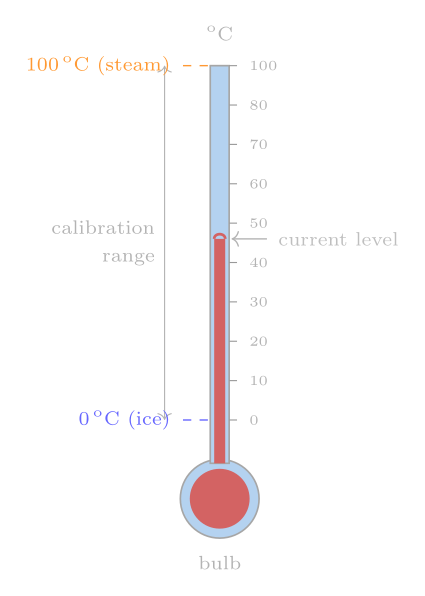
Constructing the scale requires fixed points: reproducible temperatures at which we all agree on the numerical value. Anders Celsius in 1742 chose the freezing point of water as 0 °C and the boiling point as 100 °C (his original scale was inverted, with boiling at 0 and freezing at 100 — later colleagues reversed it). Given those two anchor points, the simplest prescription is to divide the intervening column length into a hundred equal parts, assigning each one the label of one degree Celsius.
Here a subtle but important problem arises: the scale between the fixed points depends on which liquid is inside the thermometer. A mercury thermometer and an alcohol thermometer, both calibrated to agree at 0 °C and 100 °C, will disagree at intermediate temperatures because the thermal expansion coefficients of the two liquids vary with temperature in different ways. Measurements confirm this: an alcohol thermometer can read several degrees lower than mercury when both are immersed in a bath that mercury calls 50 °C. So the liquid-in-glass thermometer gives us an arbitrary, material-dependent scale. We need something better.
Constant-volume gas thermometers and absolute zero
A far more universal thermometer uses the pressure of a dilute gas confined to a fixed volume. The apparatus — a bulb containing gas connected via a manometer to a reservoir — can maintain constant volume by adjusting the height of a mercury column while reading the gas pressure. Early experimenters, following the work of Gay-Lussac and Charles, found that gases of different chemical identity (air, carbon dioxide, hydrogen) gave pressure-temperature curves that were very nearly identical when the gas was dilute enough, and that they all extrapolated to zero pressure at the same temperature, regardless of which gas was used.
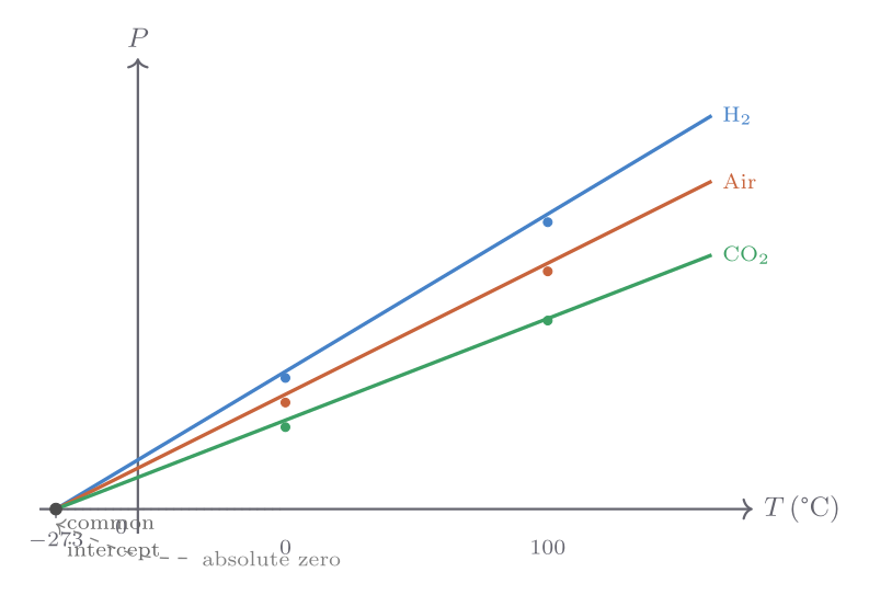
Extrapolating the pressure–temperature straight lines to zero pressure yields a common intercept at approximately \(-273.15\) °C. This is not a coincidence — it marks the point at which a classical ideal gas would have zero kinetic energy, and it defines a natural lower bound to temperature. We call this temperature absolute zero.
Shifting the origin to absolute zero gives the Kelvin scale: \(T(\text{K}) = T(°\text{C}) + 273.15\). In terms of absolute temperature the ideal-gas-thermometer relationship becomes simply
\[ PV = Nk_{\mathrm{B}}T, \]where \(N\) is the number of molecules and \(k_{\mathrm{B}} \approx 1.381 \times 10^{-23}\ \text{J K}^{-1}\) is Boltzmann’s constant. Equivalently, writing \(n\) for the number of moles and \(R = N_{\mathrm{A}} k_{\mathrm{B}} \approx 8.314\ \text{J mol}^{-1}\ \text{K}^{-1}\) for the ideal gas constant,
\[ PV = nRT. \]All four quantities — Boltzmann’s constant, Avogadro’s number \(N_{\mathrm{A}} \approx 6.022 \times 10^{23}\ \text{mol}^{-1}\), the ideal gas constant, and absolute temperature itself — are intimately linked through these two equations. The ideal gas law will serve as our operational definition of temperature throughout Part I; in Part II we will derive it from microscopic first principles.
The International Temperature Scale (ITS-90), adopted by international agreement in 1990, achieves reproducibility to better than a millikelvin by specifying a network of fixed reference points — the triple point of water at 273.16 K, the freezing points of various metals — and interpolation procedures between them. The Kelvin was formally redefined in 2019 in terms of a fixed numerical value of \(k_{\mathrm{B}}\), removing any dependence on physical artefacts.
A charming historical curiosity: Galileo thermometers exploit the temperature-dependence of fluid density rather than volume. Glass spheres of slightly different masses are sealed inside a liquid column; as temperature changes, the liquid’s density shifts and different spheres float or sink, with the lowest floating sphere indicating the temperature. The device is decorative but imprecise — a reminder that many of thermometry’s foundational concepts, including the notion of a fixed point, were worked out long before thermodynamics was a science.
Chapter 2: The Ideal Gas and the Microscopic Origin of Temperature
The ideal gas law revisited
The ideal gas law \(PV = Nk_{\mathrm{B}}T\) encodes a great deal of physics in a deceptively compact form. An ideal gas is one in which intermolecular interactions are negligible — the molecules move freely except during brief, elastic collisions. This is an excellent approximation for real gases at low densities and high temperatures, and it captures the essential behaviour that connects pressure, volume, temperature, and the amount of substance.
Before moving to a formal derivation, we should absorb what the law is saying. Pressure arises from molecular impacts on the container walls; doubling the number of molecules at fixed volume and temperature doubles the pressure. Doubling the temperature at fixed volume doubles the pressure because molecules move faster and hit harder. Doubling the volume at fixed temperature and molecule number halves the pressure because molecules strike the walls less frequently. Each of these statements is embedded in the single equation \(PV = Nk_{\mathrm{B}}T\).
Kinetic derivation of pressure and temperature
Consider a single molecule of mass \(m\) bouncing elastically between the walls of a rectangular box of length \(L\) in the \(x\)-direction. Every time the molecule strikes the right wall, it reverses its \(x\)-component of velocity from \(+v_x\) to \(-v_x\), transferring momentum \(2mv_x\) to the wall. The time between successive strikes on the same wall is \(2L/v_x\), so the average force exerted on the wall by this molecule is
\[ \bar{F}_x = \frac{2mv_x}{2L/v_x} = \frac{mv_x^2}{L}. \]For \(N\) molecules with a distribution of velocities, the total pressure on the wall of area \(A = V/L\) is
\[ P = \frac{N m \langle v_x^2 \rangle}{V}, \]where angle brackets denote an average over molecules. By isotropy — no direction is preferred — \(\langle v_x^2 \rangle = \langle v_y^2 \rangle = \langle v_z^2 \rangle = \tfrac{1}{3}\langle v^2 \rangle\), so
\[ P = \frac{2N}{3V}\left\langle \frac{1}{2}mv^2 \right\rangle = \frac{2N}{3V}\langle \epsilon_{\mathrm{kin}} \rangle. \]Comparing with the ideal gas law \(PV = Nk_{\mathrm{B}}T\) gives immediately
\[ \langle \epsilon_{\mathrm{kin}} \rangle = \frac{3}{2}k_{\mathrm{B}}T. \]This is a profound result: temperature is a measure of the mean translational kinetic energy per molecule. The factor \(\tfrac{3}{2}\) arises from the three independent spatial degrees of freedom. The total internal energy of a monatomic ideal gas of \(N\) molecules — each with no internal structure to store energy — is therefore
\[ U = \frac{3}{2}Nk_{\mathrm{B}}T. \]Two significant assumptions underlie this derivation: the collisions are elastic (no energy is lost to the walls), and all of the molecule’s energy is translational kinetic energy. For monatomic gases such as helium, neon, and argon these assumptions hold remarkably well at ordinary temperatures. For diatomic or polyatomic molecules the picture is richer: the molecule can also rotate and vibrate, storing energy in ways that do not contribute to the pressure.
Joule’s free-expansion experiment and the energy of an ideal gas
James Prescott Joule established experimentally that the internal energy of a real gas depends almost entirely on temperature and not on volume. In his famous free-expansion experiment, gas from a pressurised vessel was allowed to expand into an evacuated vessel, the whole apparatus being immersed in a water bath. Because the gas expanded into vacuum, it did no work; and Joule detected no change in the water temperature, indicating no heat flow. Since \(\Delta U = Q + W = 0\), the internal energy of the gas remained constant even though its volume doubled. The temperature also remained constant. Together these observations mean that, for an ideal gas, \(U\) depends only on \(T\) (and the fixed amount of substance), not on \(P\) or \(V\) independently. This is consistent with the kinetic result \(U = \tfrac{3}{2}Nk_{\mathrm{B}}T\) for a monatomic gas: once \(T\) is fixed, \(U\) is fixed.
The equipartition theorem and its limits
A broader empirical regularity appears when the constant-volume heat capacities of various gases are measured as a function of temperature. Monatomic gases give \(C_V = \tfrac{3}{2}Nk_{\mathrm{B}}\), diatomic gases give roughly \(\tfrac{5}{2}Nk_{\mathrm{B}}\) near room temperature and \(\tfrac{7}{2}Nk_{\mathrm{B}}\) at high temperatures, and polyatomic molecules yield still larger values. The pattern suggests a rule: each quadratic degree of freedom — one kinetic or potential energy term proportional to a coordinate or velocity squared — contributes \(\tfrac{1}{2}k_{\mathrm{B}}T\) to the mean energy and \(\tfrac{1}{2}Nk_{\mathrm{B}}\) to the heat capacity.
This is the equipartition theorem of classical statistical mechanics. For a diatomic molecule that can translate in three directions and rotate about two axes, \(f = 5\) quadratic degrees of freedom give \(U = \tfrac{5}{2}Nk_{\mathrm{B}}T\) and \(C_V = \tfrac{5}{2}Nk_{\mathrm{B}}\). At high enough temperatures vibrational modes unlock, adding two more (one kinetic, one potential per mode), raising \(f\) to 7.
The equipartition theorem is a classical result and fails dramatically when quantum effects are important. The energy spacings of rotational and vibrational levels are discrete, and at temperatures where \(k_{\mathrm{B}}T\) is much smaller than those spacings the modes are “frozen out” and do not contribute. This explains why the heat capacity of hydrogen rises in steps as temperature increases: translational modes are always active, rotational modes switch on around 100 K, and vibrational modes require several thousand kelvin. Equipartition should therefore be regarded as a useful approximation valid in specific temperature ranges rather than an exact theorem. Its proper derivation and limits are the subject of a full statistical-mechanics course; here we use its results empirically, taking \(C_V = \tfrac{3}{2}Nk_{\mathrm{B}}\) for noble gases and \(C_V \approx \tfrac{5}{2}Nk_{\mathrm{B}}\) for air near room temperature.
Chapter 3: The First Law, Work, and Heat Capacities
The first law of thermodynamics
Energy is conserved. For a thermodynamic system, energy can change in two ways: by heat flowing across its boundary, or by work being done on or by it. Writing \(Q\) for the heat flowing into the system and \(W\) for the work done on the system, the first law states
\[ \Delta U = Q + W. \]Several subtleties of notation deserve emphasis. Heat \(Q\) and work \(W\) are not properties of the system’s state — they describe processes, not states. There is no such thing as “the heat content” of a gas; there is only the heat that has flowed during a particular change. For this reason, writing the first law as \(\Delta U = \Delta Q + \Delta W\) is misleading, and the more careful notation with plain \(Q\) and \(W\) (understood as finite quantities associated with a process) is preferred. An infinitesimal version is often written \(dU = \delta Q + \delta W\), where the Greek \(\delta\) signals that \(\delta Q\) and \(\delta W\) are not exact differentials — they depend on the path taken, not just on the initial and final states.
Expansion and compression work
When a gas expands quasi-statically against an external pressure, it does work on its surroundings. Quasi-static means the process passes through a continuous sequence of equilibrium states: the gas pressure remains well-defined throughout. Under this condition, the work done on the gas in a volume change \(dV\) is
\[ \delta W = -P\,dV, \]with the sign convention that compression (\(dV < 0\)) is positive work done on the gas. For a finite quasi-static process,
\[ W = -\int_{V_i}^{V_f} P\,dV. \]On a pressure-volume indicator diagram — a plot of \(P\) versus \(V\) — the work done by the gas in going from state \(i\) to state \(f\) is the area under the curve. A crucial lesson: this area, and hence \(W\), depends on the path taken in \(PV\)-space, not just on the endpoints.
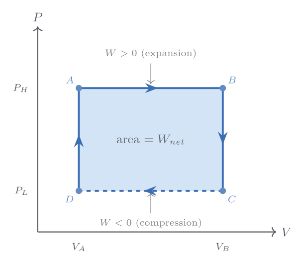
The path-dependence of work becomes vivid when we compare three ways of taking an ideal gas from a state \((P_i, V_i)\) to a state \((P_i/2,\, 2V_i)\) — the same initial and final temperatures since \(T = PV/Nk_{\mathrm{B}}\) is unchanged. Along an isotherm the work done on the gas is \(W = -Nk_{\mathrm{B}}T\ln 2 \approx -0.69\,Nk_{\mathrm{B}}T\); along the path of constant volume followed by constant pressure it is \(-Nk_{\mathrm{B}}T/2\); and along constant pressure followed by constant volume it is \(-Nk_{\mathrm{B}}T\). The internal energy change \(\Delta U = 0\) in all three cases (since \(\Delta T = 0\) for an ideal gas), but \(Q = -W\) takes three different values. This concretely demonstrates that \(Q\) and \(W\) are properties of the process, not of the states.
Non-quasi-static processes — such as Joule’s free expansion into vacuum — cannot be represented as paths on an indicator diagram because the pressure is not well-defined during the process. Such processes are indicated by dotted lines connecting the well-defined initial and final states.
Isothermal and adiabatic processes
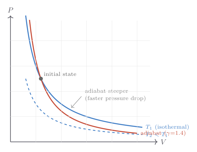
An isothermal process maintains constant temperature. For an ideal gas, \(PV = Nk_{\mathrm{B}}T = \text{const}\), so the indicator-diagram curve is a hyperbola \(P \propto V^{-1}\). Since \(\Delta U = 0\) for isothermal changes of an ideal gas, all heat flowing in exactly balances the work done by the gas: \(Q = -W = Nk_{\mathrm{B}}T\ln(V_f/V_i)\).
An adiabatic process allows no heat exchange: \(\delta Q = 0\). This can be achieved either by thermally insulating the system or by performing the process so rapidly that heat has no time to flow. When a gas is compressed adiabatically it heats up; when it expands it cools — phenomena familiar in the firing of a fire syringe (rapid compression of air ignites tinder) and in the cooling of rising air masses in meteorology.
For a quasi-static adiabatic process on an ideal gas with constant heat-capacity ratio \(\gamma = C_P/C_V\), the first law gives \(C_V\,dT = -P\,dV\), which together with the ideal gas law integrates to the adiabat relations:
\[ TV^{\gamma-1} = \text{const}, \qquad PV^{\gamma} = \text{const}. \]Since \(\gamma > 1\) always, adiabats are steeper than isotherms on a \(PV\) diagram — the gas cools faster than it would need to in order to maintain temperature. This steepness has a famous application: Newton computed the speed of sound assuming isothermal compression and obtained the wrong answer; Laplace’s correction using adiabatic compression (since sound waves oscillate too fast for heat to flow) gave the right result, \(v_s = \sqrt{\gamma P/\rho}\).
Internal energy and heat capacities
The heat capacity at constant volume is defined as the ratio of heat flow to temperature change under conditions of constant volume (so that no work is done):
\[ C_V = \left(\frac{\partial U}{\partial T}\right)_V. \]For a monatomic ideal gas, \(C_V = \tfrac{3}{2}Nk_{\mathrm{B}}\). For air (predominantly diatomic \(\mathrm{N_2}\) and \(\mathrm{O_2}\) near room temperature), \(C_V \approx \tfrac{5}{2}Nk_{\mathrm{B}}\).
The heat capacity at constant pressure \(C_P\) is more relevant for laboratory experiments on gases and for all work with condensed phases (solids and liquids), where constant volume is difficult to enforce. Under constant pressure, the first law gives
\[ Q = \Delta U + P\Delta V = \Delta H, \]where \(H \equiv U + PV\) is the enthalpy (discussed in Chapter 5). Hence
\[ C_P = \left(\frac{\partial H}{\partial T}\right)_P. \]For an ideal gas, Joule’s result that \(U\) depends only on \(T\) means \((\partial U/\partial T)_P = (\partial U/\partial T)_V = C_V\). The extra work term when the gas expands at constant pressure contributes \(P(\partial V/\partial T)_P = Nk_{\mathrm{B}}\), giving the Mayer relation:
\[ C_P - C_V = Nk_{\mathrm{B}} \quad \text{(ideal gas)}. \]This is not an approximation for an ideal gas — it is exact. For a real substance the general relation is \(C_P - C_V = TV\beta^2/\kappa_T\), where \(\beta = (1/V)(\partial V/\partial T)_P\) is the isobaric thermal expansivity and \(\kappa_T = -(1/V)(\partial V/\partial P)_T\) is the isothermal compressibility. For solids and liquids, \(\beta\) and \(\kappa_T\) are small, so \(C_P \approx C_V\) — the difference is typically a few percent of \(C_V\) near room temperature for crystalline solids. For gases, the Mayer correction is significant: for air, \(C_P/C_V = \gamma \approx 1.40\).
As a numerical example, for copper at 298 K: \(\beta = 5.0 \times 10^{-5}\ \text{K}^{-1}\), \(\kappa_T = 7.2 \times 10^{-12}\ \text{Pa}^{-1}\), molar volume \(V_m = 7.1 \times 10^{-6}\ \text{m}^3\text{mol}^{-1}\), and \(C_V = 22.6\ \text{J mol}^{-1}\text{K}^{-1}\). The correction is \(TV_m\beta^2/\kappa_T = 298 \times 7.1\times10^{-6} \times (5\times10^{-5})^2 / (7.2\times10^{-12}) \approx 0.73\ \text{J mol}^{-1}\text{K}^{-1}\), giving \(C_P \approx 24.5\ \text{J mol}^{-1}\text{K}^{-1}\) — a 3.2% correction, in agreement with the tabulated value of \(24.4\ \text{J mol}^{-1}\text{K}^{-1}\).
The general relation \(C_P - C_V = TV\beta^2/\kappa_T\) has an important consequence: since \(\beta^2 \geq 0\) and \(\kappa_T \geq 0\) (matter is mechanically stable), we always have \(C_P \geq C_V\). This is a thermodynamic stability condition, not an accident.
Deriving \(C_P - C_V = Nk_{\mathrm{B}}\) for an ideal gas
The Mayer relation deserves a careful derivation, because the argument is frequently glossed over. Starting from the definition \(C_P - C_V = (\partial H/\partial T)_P - (\partial U/\partial T)_V\), substitute \(H = U + PV\):
\[ C_P - C_V = \left(\frac{\partial U}{\partial T}\right)_P + P\left(\frac{\partial V}{\partial T}\right)_P - \left(\frac{\partial U}{\partial T}\right)_V. \]The first and third terms are not identical because \(U\) is evaluated at constant \(P\) and constant \(V\) respectively. Using the chain rule for \(U(T, V)\) evaluated at constant \(P\):
\[ \left(\frac{\partial U}{\partial T}\right)_P = \left(\frac{\partial U}{\partial T}\right)_V + \left(\frac{\partial U}{\partial V}\right)_T \left(\frac{\partial V}{\partial T}\right)_P. \]Substituting and collecting terms:
\[ C_P - C_V = \left[\left(\frac{\partial U}{\partial V}\right)_T + P\right]\left(\frac{\partial V}{\partial T}\right)_P. \]For an ideal gas, Joule’s free-expansion experiment established \((\partial U/\partial V)_T = 0\). The remaining factor is \(P(\partial V/\partial T)_P\). With \(V = Nk_{\mathrm{B}}T/P\), differentiation gives \((\partial V/\partial T)_P = Nk_{\mathrm{B}}/P\), and therefore
\[ C_P - C_V = P \cdot \frac{Nk_{\mathrm{B}}}{P} = Nk_{\mathrm{B}}. \]For a non-ideal substance, the internal pressure \((\partial U/\partial V)_T\) is not zero — it quantifies how intermolecular attractions store potential energy when the substance is expanded. In Chapter 18 the Maxwell relation \((\partial U/\partial V)_T = T(\partial P/\partial T)_V - P\) will be used to express this internal pressure in terms of measurable \(P\)–\(V\)–\(T\) derivatives, yielding the general formula \(C_P - C_V = TV\beta^2/\kappa_T\).
The heat-capacity ratio \(\gamma\) and its physical meaning
The dimensionless ratio \(\gamma \equiv C_P/C_V\) appears in nearly every formula involving adiabatic processes. For monatomic ideal gases \(\gamma = 5/3 \approx 1.667\); for diatomic gases near room temperature \(\gamma = 7/5 = 1.4\); for polyatomic gases with many modes \(\gamma \to 1\) from above. The significance of \(\gamma\) is most transparent in the adiabatic relations. When an ideal gas is compressed adiabatically, the first law gives \(C_V\,dT = -P\,dV\). Using the ideal gas law to eliminate \(P\) and integrating yields \(TV^{\gamma-1} = \text{const}\). Rewriting in terms of pressure: since \(T = PV/(Nk_{\mathrm{B}})\), one obtains \(PV^\gamma = \text{const}\).
The ratio \(\gamma\) also controls the speed of sound in an ideal gas. Newton originally computed the sound speed as \(v_s = \sqrt{P/\rho}\), assuming isothermal compression. Laplace corrected this by noting that acoustic oscillations are so rapid that heat has no time to flow between compression and rarefaction zones — they are adiabatic. The corrected result is \(v_s = \sqrt{\gamma P/\rho} = \sqrt{\gamma k_{\mathrm{B}}T/m}\), where \(m\) is the molecular mass. For air at 293 K with \(\gamma = 1.40\) and \(m = 29 \times 1.66 \times 10^{-27}\ \text{kg}\), this gives \(v_s \approx 343\ \text{m s}^{-1}\), in excellent agreement with measurement.
Worked example: isothermal and adiabatic processes
Isothermal expansion. One mole of an ideal diatomic gas (\(C_V = \tfrac{5}{2}R\), \(C_P = \tfrac{7}{2}R\), \(\gamma = 1.4\)) at \(T = 300\ \text{K}\) and \(P_i = 2\ \text{atm}\) expands isothermally to \(P_f = 1\ \text{atm}\). Since temperature is fixed, \(U\) does not change. The work done by the gas is \(W_\text{by} = nRT\ln(V_f/V_i) = nRT\ln(P_i/P_f) = (1)(8.314)(300)\ln 2 \approx 1730\ \text{J}\). All of this work is supplied by heat flowing in: \(Q = 1730\ \text{J}\).
Adiabatic compression. Now suppose the gas at \(T_i = 300\ \text{K}\), \(P_i = 1\ \text{atm}\) is compressed adiabatically by a factor \(V_i/V_f = 10\) (compression ratio \(r = 10\)). The final temperature follows from \(TV^{\gamma-1} = \text{const}\):
\[ T_f = T_i \left(\frac{V_i}{V_f}\right)^{\gamma-1} = 300 \times 10^{0.4} \approx 300 \times 2.512 \approx 754\ \text{K}. \]The temperature rises by 454 K purely from compression — no heat is added. The final pressure is \(P_f = P_i(V_i/V_f)^\gamma = 1 \times 10^{1.4} \approx 25.1\ \text{atm}\). The work done on the gas equals the increase in internal energy: \(W = \Delta U = nC_V(T_f - T_i) = (1)(\tfrac{5}{2} \times 8.314)(454) \approx 9430\ \text{J}\). This large quantity of work stored as internal energy is the principle behind diesel ignition: air compressed to a ratio of 15:1 reaches temperatures around 800–900 K, sufficient to ignite injected fuel without a spark.
Physical difference between \(C_P\) and \(C_V\) experiments
Measuring \(C_V\) at constant volume requires a rigid container — straightforward for liquids (place sample in a sealed bomb calorimeter), but mechanically demanding for gases under pressure, and essentially impossible for a gas that must remain at low pressure while spanning a large temperature range. In practice, gas heat capacities are almost always measured at constant pressure (typically atmospheric), and \(C_V\) is obtained by subtraction using the Mayer relation. For solids and liquids, maintaining strict constant volume is so difficult that \(C_P\) is measured and the difference \(TV\beta^2/\kappa_T\) (typically 1–5 % of \(C_V\) for crystalline solids near room temperature) is subtracted to get \(C_V\). This general formula thus has direct experimental utility beyond its aesthetic elegance.
Chapter 4: Phase Transitions and Latent Heat
What is a phase?
Ordinary matter appears in distinct phases: solid, liquid, and gas (and less familiar phases such as plasma and superfluid). Within a given phase, macroscopic properties such as density and compressibility vary smoothly with temperature and pressure. At a phase transition, properties can change discontinuously — ice melts at a sharp temperature, and the density jumps from roughly \(917\ \text{kg/m}^3\) to \(1000\ \text{kg/m}^3\).
The clearest way to approach phase transitions is to start with the ideal gas law and ask where it breaks down. Consider the isotherms of real nitrogen (\(\mathrm{N_2}\)) on a \(P\)–\(V\) diagram. At high temperatures and large volumes, the ideal gas law \(P = Nk_{\mathrm{B}}T/V\) is an excellent description. As the temperature drops or the pressure rises, the actual pressure at a given volume falls below the ideal prediction — intermolecular attractions pull the molecules together slightly. At low enough temperatures, something dramatic occurs: as the gas is compressed at constant temperature, the pressure stops changing over a finite range of volumes. During this pressure plateau, liquid is forming from gas; the two phases coexist in equilibrium, and the volume decreases as more gas condenses into denser liquid. Only when all gas has condensed does the pressure rise steeply again.
This constant-pressure plateau — a first-order phase transition — disappears above the critical temperature \(T_c\). Above \(T_c\), no amount of pressure can force the fluid to condense discontinuously; there is a single fluid phase that connects smoothly between what we might call gas and liquid. Nitrogen has \(T_c \approx 126\ \text{K}\), \(P_c \approx 3.4\ \text{MPa}\). This means liquid nitrogen cannot exist above 126 K at any pressure — an important fact for cryogenic applications.
A gas can be continuously transformed into a liquid by skirting around the critical point in \(P\)–\(T\) space, never crossing the phase boundary. This reveals that liquids and gases are not fundamentally different phases — they are continuously connected. Solids, however, are fundamentally different: in the solid phase, atoms or molecules are fixed in their relative positions, and no continuous path in \(P\)–\(T\) space connects solid to fluid without crossing a phase boundary.
Latent heat
At a first-order phase transition such as melting or vaporisation, heat flows into (or out of) the system at constant temperature and pressure. This heat, the latent heat \(L\), is associated with the rearrangement of molecular bonds rather than a change in kinetic energy. The temperature remains constant during the transition because the added thermal energy is used to break bonds (increasing potential energy) rather than to increase the kinetic energy of molecules. This behaviour is fundamentally different from what the equipartition theorem would predict for a smooth, single-phase substance — it is a signature of the discrete, discontinuous nature of first-order phase transitions. For fusion (solid \(\to\) liquid) and vaporisation (liquid \(\to\) gas):
| Substance | \(L_\text{fus}\ (\text{kJ/mol})\) | \(L_\text{vap}\ (\text{kJ/mol})\) |
|---|---|---|
| Water | 6.01 | 40.7 |
| Nitrogen | 0.72 | 5.57 |
| Iron | 13.8 | 340 |
| Helium-4 | 0.021 | 0.083 |
Vaporisation latent heats are typically much larger than fusion latent heats, because converting a liquid to a gas requires breaking most intermolecular bonds, while melting only partially disorders the structure.
At constant pressure, the heat required to melt a mass \(m\) of a substance is \(Q = mL_\text{fus}\), where \(L_\text{fus}\) is the specific latent heat (per kilogram). Since this occurs at constant pressure, it equals the enthalpy change: \(\Delta H_\text{fus} = mL_\text{fus}\). The entropy change at a first-order transition is
\[ \Delta S = \frac{Q}{T_\text{transition}} = \frac{\Delta H}{T_\text{transition}}. \]For the melting of one mole of ice at 273 K, \(\Delta S = 6010/273 \approx 22\ \text{J mol}^{-1}\text{K}^{-1}\). Entropy increases on melting, as expected — the liquid has far more accessible microstates than the ordered crystal.
A remarkable demonstration of thermal physics involves the fire syringe: a tightly fitting piston rapidly compresses a small volume of air. The adiabatic temperature rise — which, for a compression ratio of 10:1 with \(\gamma = 1.4\), brings the temperature from 300 K to about 753 K — is sufficient to ignite a piece of tinder placed inside. The device was known in Southeast Asia long before the invention of matches.
The phase diagram and the triple point
The two-dimensional \(P\)–\(T\) plane provides the most economical representation of the stable phases of a single-component substance. Each region of this phase diagram corresponds to a single stable phase; the boundaries between regions are the curves along which two phases coexist in equilibrium. Three such curves meet at a single invariant point — the triple point — where all three phases coexist simultaneously. For water, the triple point occurs at \(T_\text{tp} = 273.16\ \text{K}\) and \(P_\text{tp} = 611.7\ \text{Pa}\). It is used as the primary thermometric fixed point in the International Temperature Scale because, unlike the melting and boiling points at 1 atm, the triple point is independent of external pressure.
Above the critical point \((T_c, P_c)\), the liquid–gas phase boundary terminates and there is no longer a discontinuous distinction between liquid and gas. For water, \(T_c = 647.1\ \text{K}\) and \(P_c = 218\ \text{atm}\); for carbon dioxide, \(T_c = 304.1\ \text{K}\) and \(P_c = 72.8\ \text{atm}\). This means that \(\mathrm{CO_2}\) has a reachable critical point at temperatures accessible in a laboratory, making it easy to observe critical opalescence and supercritical fluid behaviour.
The Clausius-Clapeyron equation — a preview
The slope of any phase boundary in the \(P\)–\(T\) plane is not arbitrary; it is governed by the thermodynamic condition \(\mu_\alpha(T,P) = \mu_\beta(T,P)\), which must hold along the entire boundary. Differentiating this condition with respect to \(T\) along the boundary, and using \(d\mu = -S_m\,dT + V_m\,dP\) (where \(S_m\) and \(V_m\) are molar entropy and volume), one obtains the Clausius-Clapeyron equation:
\[ \frac{dP}{dT}\bigg|_\text{coexistence} = \frac{\Delta S_m}{\Delta V_m} = \frac{L}{T\Delta V_m}, \]where \(L = T\Delta S_m\) is the molar latent heat and \(\Delta V_m = V_m^\beta - V_m^\alpha\) is the molar volume difference between the two phases. This equation is derived in full detail in Chapter 19; here it explains the qualitative features of phase diagrams.
Why water’s melting curve has a negative slope
For almost every pure substance, the solid phase is denser than the liquid at the melting point, so \(\Delta V_m = V_m^\text{liq} - V_m^\text{solid} > 0\). Since \(L > 0\) always (melting absorbs heat), the Clausius-Clapeyron slope is positive: raising the pressure raises the melting temperature. Water is famous for its anomalous behaviour: ice at 0 °C has density \(917\ \text{kg m}^{-3}\) while liquid water has density \(1000\ \text{kg m}^{-3}\), so \(\Delta V_m < 0\) and \(dP/dT|_\text{melt} \approx -13.5\ \text{MPa K}^{-1}\). Increasing pressure by 1 atm lowers the melting point by only 0.0074 K — far too small to explain ice skating, which requires cooling of several degrees. The anomaly arises because ice forms an open hydrogen-bonded network (the wurtzite-type crystal structure of hexagonal ice) that collapses to a denser arrangement upon melting, unlike close-packed crystals.
The negative slope of water’s melting curve also means that, below the triple point, one cannot liquefy water by pressure alone — instead ice sublimes directly to vapour. This is why freeze-drying works: food is cooled below the triple-point temperature and placed in a low-pressure chamber so that ice sublimes without passing through the liquid phase, preserving texture and nutritional value.
More on latent heat physics
Latent heat reflects a fundamental competition between entropy and internal energy at the molecular level. At the melting point, the solid and liquid have equal Gibbs free energies: \(G_\text{solid} = G_\text{liq}\), meaning \(U_\text{solid} - TS_\text{solid} + PV_\text{solid} = U_\text{liq} - TS_\text{liq} + PV_\text{liq}\). Rearranging: \(L = T\Delta S = \Delta U + P\Delta V\). Most of the latent heat of fusion goes into breaking the rigid crystal lattice’s directional bonds (the \(\Delta U\) term), with a smaller contribution from the volume change \(P\Delta V\). For vaporisation, the dominant term is the intermolecular potential energy: bringing a molecule from the bulk liquid to the vapour requires breaking essentially all its close-range interactions, each of order \(\epsilon \sim k_{\mathrm{B}}T_\text{boil}\), with roughly \(z/2 \sim 5\) nearest neighbours. This gives a rough estimate \(L_\text{vap} \sim 5 N_A k_{\mathrm{B}} T_\text{boil}\), or about \(5RT_\text{boil}\) per mole. For water (\(T_\text{boil} = 373\ \text{K}\)), this gives \(L_\text{vap} \sim 5 \times 8.314 \times 373 \approx 15.5\ \text{kJ mol}^{-1}\), somewhat below the actual value of \(40.7\ \text{kJ mol}^{-1}\) because water’s hydrogen bonds are unusually strong. The ratio \(L_\text{vap}/L_\text{fus}\) is typically 6–10 for most substances, reflecting the larger disruption of intermolecular order in vaporisation than in melting.
Chapter 5: Enthalpy and Chemical-Reaction Energetics
Definition and motivation
The enthalpy is the combination
\[ H \equiv U + PV, \]which might at first look like an unmotivated algebraic construction. Its utility becomes clear in constant-pressure processes. When a system at constant pressure \(P_0\) changes state, the heat flowing in is
\[ Q_P = \Delta U + P_0 \Delta V = \Delta U + \Delta(P_0 V) = \Delta H. \]So enthalpy change equals heat flow at constant pressure (provided no non-\(PV\) work is done). Since most laboratory chemistry and engineering occurs at atmospheric pressure, enthalpy is the natural thermodynamic potential for thermal processes in open vessels.
Enthalpy is a state function — it depends only on the current state of the system, not on how the system got there. This makes enthalpy changes additive and tabulated: to find the heat released in a complex reaction, one can combine tabulated enthalpy changes of simpler reactions. This is Hess’s law, a direct consequence of enthalpy being a state function.
Throttling and the Joule-Thomson process
A particularly elegant application of enthalpy arises in throttling (the Joule-Thomson process): a gas is forced through a porous plug or narrow valve from high pressure \(P_i\) to low pressure \(P_f\), with insulating walls so \(Q = 0\). Work done by the gas on both sides of the throttle gives
\[ W = P_i V_i - P_f V_f, \qquad \therefore\; \Delta U = P_i V_i - P_f V_f, \]which rearranges to \(U_f + P_f V_f = U_i + P_i V_i\), i.e., enthalpy is conserved in throttling: \(\Delta H = 0\). For an ideal gas, \(H = U + PV = U + Nk_{\mathrm{B}}T\) depends only on temperature, so \(\Delta H = 0\) implies \(\Delta T = 0\): throttling an ideal gas produces no temperature change. Real gases do cool or warm slightly because their internal energy has a weak volume-dependence. The Joule-Thomson coefficient
\[ \mu_{\mathrm{JT}} = \left(\frac{\partial T}{\partial P}\right)_H \]is positive (cooling on expansion) below an inversion temperature and negative above it. For most common gases at room temperature \(\mu_{\mathrm{JT}} > 0\), which is why throttling is used in refrigerators and liquefiers — the Linde process for liquefying air relies on it.
Enthalpies of formation and chemical reactions
The enthalpy of formation \(\Delta_f H^\circ\) of a substance is defined as the enthalpy change when one mole of the substance is produced from its elemental constituents in their standard states (298 K, 1 bar). By convention, elemental substances in their standard forms (H\(_2\)(g), O\(_2\)(g), Fe(s), etc.) have \(\Delta_f H^\circ = 0\).
For the formation of liquid water: \(\text{H}_2(\text{g}) + \tfrac{1}{2}\text{O}_2(\text{g}) \to \text{H}_2\text{O}(\ell)\), \(\Delta_f H^\circ = -286\ \text{kJ mol}^{-1}\). The negative sign means heat is released — this is an exothermic reaction. For any reaction, Hess’s law gives the total enthalpy change as the sum of formation enthalpies of products minus those of reactants:
\[ \Delta_r H^\circ = \sum_\text{products} \Delta_f H^\circ - \sum_\text{reactants} \Delta_f H^\circ. \]This \(\Delta_r H^\circ\) equals the heat released to the surroundings (at constant pressure, with no electrical or other non-\(PV\) work). When a battery is discharging, electrical work is also done, and the heat released is less than \(\Delta_r H^\circ\) — a point to keep in mind when comparing fuel combustion to electrochemical cells.
Why enthalpy is the correct variable for constant-pressure chemistry
Almost all laboratory chemistry takes place in open vessels exposed to atmospheric pressure. The experimenter typically cares only about the heat released or absorbed — not about the mechanical work done on the atmosphere when gas is produced or consumed. Enthalpy captures precisely this quantity: the heat flow at constant pressure, regardless of the volume change.
Consider the combustion of methane: \(\mathrm{CH_4(g) + 2\,O_2(g) \to CO_2(g) + 2\,H_2O(l)}\). The moles of gas decrease from 3 to 1. At 298 K and 1 bar, the volume decrease \(\Delta V = (1-3) \times RT/P = -2RT/P\) corresponds to a work done on the gas of \(P|\Delta V| = 2RT \approx 4.96\ \text{kJ mol}^{-1}\). The internal energy change is \(\Delta_r U^\circ = -890.3 + 4.96 \approx -885.3\ \text{kJ mol}^{-1}\), while the tabulated enthalpy change is \(\Delta_r H^\circ = -890.3\ \text{kJ mol}^{-1}\). For a calorimetric measurement in an open vessel, it is \(\Delta_r H^\circ\) that appears directly as the heat released; isolating \(\Delta_r U^\circ\) requires a rigid-walled bomb calorimeter. Both quantities are physically meaningful, but enthalpy is the one directly accessible in open-vessel experiments.
Hess’s law as a consequence of enthalpy being a state function
The power of Hess’s law goes beyond simple additive bookkeeping. Because \(H\) is a state function, the enthalpy change for any chemical transformation is independent of the path taken — regardless of what intermediates the reaction passes through, what mechanisms are operative, or even whether the direct reaction is experimentally feasible. This means that reactions which are too fast, too slow, or too dangerous to study calorimetrically can have their enthalpies determined indirectly by combining the enthalpies of related measurable reactions.
A classic application: the enthalpy of formation of carbon monoxide, \(\text{C(s)} + \tfrac{1}{2}\text{O}_2(\text{g}) \to \text{CO(g)}\), is difficult to measure directly because carbon also burns to \(\text{CO}_2\). Using known values \(\Delta_f H^\circ[\text{CO}_2] = -393.5\ \text{kJ mol}^{-1}\) and \(\Delta_\text{comb} H^\circ[\text{CO}] = -283.0\ \text{kJ mol}^{-1}\) (combustion of CO to \(\text{CO}_2\)):
\[ \Delta_f H^\circ[\text{CO}] = \Delta_f H^\circ[\text{CO}_2] - \Delta_\text{comb} H^\circ[\text{CO}] = -393.5 - (-283.0) = -110.5\ \text{kJ mol}^{-1}. \]This value, inaccessible by direct experiment, is central to industrial chemistry — the water-gas shift reaction and Fischer-Tropsch synthesis both involve CO, and knowing \(\Delta_f H^\circ[\text{CO}]\) is essential for energy accounting.
Worked enthalpy calculation: combustion of octane
Octane (\(\mathrm{C_8H_{18}}\), the primary component of gasoline) combusts as \(\mathrm{C_8H_{18}(l) + \tfrac{25}{2}\,O_2(g) \to 8\,CO_2(g) + 9\,H_2O(l)}\). Using standard enthalpies of formation:
\[ \Delta_r H^\circ = [8 \times (-393.5) + 9 \times (-285.8)] - [(-250.1) + 0] = [-3148 - 2572.2] - [-250.1] \]\[ = -5720.2 + 250.1 = -5470.1\ \text{kJ mol}^{-1}. \]The molar mass of octane is \(114.2\ \text{g mol}^{-1}\), giving a specific energy of \(5470/114.2 \approx 47.9\ \text{kJ g}^{-1}\). This compares well with the tabulated lower heating value of gasoline (\(\approx 44\ \text{MJ kg}^{-1}\)), with the discrepancy reflecting the mixture composition and the fact that the “lower” heating value assumes water leaves as vapour rather than liquid. The enormous enthalpy change per mole — more than 5 MJ — reflects the very large number of C–H and C–C bonds being replaced by the stronger C=O bonds in \(\text{CO}_2\) and O–H bonds in water.
Chapter 6: Thermal Conduction and Fourier’s Law
Mechanisms of heat transport
Heat moves between regions of differing temperature by three mechanisms: conduction, in which energy is transferred by molecular collisions through a stationary medium; convection, in which a fluid carries heat by bulk motion; and radiation, in which electromagnetic waves transport energy without need of a material medium. In this chapter we focus on conduction; radiation is the subject of Part VI.
Fourier’s law
Fourier’s law of heat conduction (1822) states that the rate of heat flow per unit area through a medium is proportional to the local temperature gradient and directed down the gradient:
\[ \mathbf{j}_Q = -\kappa_\text{th}\,\nabla T, \]where \(\mathbf{j}_Q\) is the heat-flux vector (watts per square metre) and \(\kappa_\text{th}\) is the thermal conductivity of the material (W m\(^{-1}\) K\(^{-1}\)). In one dimension,
\[ \dot{Q} = -\kappa_\text{th} A \frac{dT}{dx}, \]where \(\dot{Q}\) is the heat current (watts) through cross-section \(A\). The minus sign ensures that heat flows from hot to cold: a positive temperature gradient in the \(x\)-direction drives a negative (leftward) heat flux.
The thermal conductivities of common materials span orders of magnitude:
| Material | \(\kappa_\text{th}\ (\text{W m}^{-1}\text{K}^{-1})\) |
|---|---|
| Diamond | 2000 |
| Copper | 400 |
| Aluminium | 237 |
| Glass | 0.8 |
| Water | 0.6 |
| Wood | 0.1 |
| Air | 0.026 |
| Aerogel | 0.015 |
The enormous range — from diamond (the best thermal conductor known, used in heat sinks for high-power electronics) to aerogel (approaching the conductivity of the air it contains) — reflects the wide variety of microscopic heat-transport mechanisms. In metals, conduction electrons carry most of the heat; in insulators, lattice vibrations (phonons) carry it; in porous materials, the entrapped gas dominates.
The contrast between water and air explains a practical hazard: falling into cold water at 5 °C is far more dangerous than standing in air at the same temperature, because water conducts heat away from the body roughly 25 times faster. The thermal conductivities also reflect the underlying physics of heat transport: in metals, the dominant carriers are conduction electrons, which have much higher mean free paths than phonons in insulators. The Wiedemann-Franz law states that the ratio of thermal conductivity to electrical conductivity is proportional to temperature: \(\kappa_\text{th}/\sigma_\text{el} = LT\), where \(L = \pi^2 k_{\mathrm{B}}^2/(3e^2) \approx 2.44 \times 10^{-8}\ \text{W}\Omega\text{K}^{-2}\) is the Lorenz number. Good electrical conductors (copper, silver) are therefore also excellent thermal conductors — explaining why copper water pipes are hot to the touch near a heating element.
Heat conduction through composite slabs
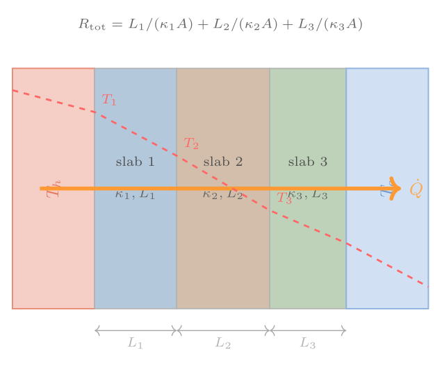
In steady state, the heat flux \(\dot{Q}/A\) must be the same throughout a series of layers — otherwise energy would be accumulating somewhere. For a composite slab of \(n\) layers with thermal conductivities \(\kappa_i\) and thicknesses \(L_i\), equating the heat flux in each layer and summing gives
\[ \frac{\dot{Q}}{A} = \frac{T_\text{hot} - T_\text{cold}}{\displaystyle\sum_{i=1}^{n} \frac{L_i}{\kappa_i}} = \frac{\Delta T}{\sum_i R_i}, \]where the thermal resistance (R-value) of each layer is \(R_i = L_i/\kappa_i\). Resistances in series add — exactly analogously to electrical resistors in series. This analogy with electrical circuits is not coincidental: both Fourier’s law and Ohm’s law are linear transport laws of the same mathematical form.
A double-glazed window illustrates the power of this formula. A single 3.2 mm pane of glass (\(\kappa = 0.8\ \text{W m}^{-1}\text{K}^{-1}\)) has \(R = 4 \times 10^{-3}\ \text{m}^2\text{K W}^{-1}\); it admits roughly 5 kW through each square metre at a 20 K indoor-outdoor temperature difference. Adding two thin still-air layers (1 mm each, \(\kappa = 0.026\)) raises the total R-value to about \(8 \times 10^{-3}\ \text{m}^2\text{K W}^{-1}\) and halves the heat loss. A proper double-glazed unit with a vacuum gap does far better still. R-values quoted on commercial insulation are just the ratios \(L/\kappa\) for the insulating product, directly comparable by simple addition.
Kinetic-theory underpinning of thermal conductivity
Fourier’s law is a macroscopic statement; its microscopic foundation is kinetic theory. In a dilute gas, molecules travel freely between collisions. Those coming from a hotter region carry more energy, on average, than those from a cooler region. The net energy flux turns out to be
\[ \kappa_\text{th} = \frac{1}{3}\,\bar{v}\,\lambda\,\frac{C_V}{V}, \]where \(\bar{v}\) is the mean molecular speed, \(\lambda\) the mean free path (average distance between collisions), and \(C_V/V\) the heat capacity per unit volume. This expression, derived properly in Chapter 12, captures the key physics: better thermal conductors have faster molecules, longer free paths, or larger heat capacities per unit volume. The mean free path \(\lambda \sim 1/(n\sigma)\), where \(n\) is the number density and \(\sigma\) the collision cross-section, introduces the density-dependence. Halving the pressure halves \(n\), doubles \(\lambda\), and leaves \(\kappa_\text{th}\) unchanged — a somewhat counterintuitive but experimentally verified result. Only at very low pressures, when \(\lambda\) becomes comparable to the container size, does \(\kappa_\text{th}\) finally start to decrease with pressure. This is why vacuum insulation works: at pressures below about 0.1 Pa (where \(\lambda\) exceeds the gap width in a vacuum panel), the gas thermal conductivity drops effectively to zero, and the only remaining heat transfer mechanisms are radiation across the evacuated gap and solid conduction through the thin support structure. Vacuum-insulated panels achieve effective thermal conductivities of \(0.004–0.006\ \text{W m}^{-1}\text{K}^{-1}\), an order of magnitude below aerogel and nearly 200 times better than glass.
Multi-layer composite slabs and the R-value
The result for a composite slab of \(n\) layers deserves a more explicit derivation. In steady state, energy conservation requires the heat current \(\dot{Q}\) to be the same in every layer. For layer \(i\) with conductivity \(\kappa_i\), thickness \(L_i\), and cross-sectional area \(A\), Fourier’s law gives \(\dot{Q} = \kappa_i A\,\Delta T_i / L_i\), where \(\Delta T_i\) is the temperature drop across layer \(i\). Solving for each temperature drop: \(\Delta T_i = \dot{Q} L_i / (\kappa_i A)\). The total temperature difference across all layers is the sum:
\[ \Delta T_\text{total} = \sum_{i=1}^n \Delta T_i = \frac{\dot{Q}}{A}\sum_{i=1}^n \frac{L_i}{\kappa_i}. \]Inverting to get \(\dot{Q}\):
\[ \dot{Q} = A\,\frac{\Delta T_\text{total}}{\displaystyle\sum_{i=1}^n R_i}, \qquad R_i \equiv \frac{L_i}{\kappa_i}, \]where \(R_i\) has units of \(\text{m}^2\text{ K W}^{-1}\). In the building industry, thermal resistance is commonly quoted as the RSI value in SI units (or the R-value in imperial units, \(1\ \text{ft}^2\text{°F·hr/Btu} = 0.176\ \text{m}^2\text{K W}^{-1}\)). A well-insulated wall with fibreglass batts (\(L = 14\ \text{cm}\), \(\kappa \approx 0.045\ \text{W m}^{-1}\text{K}^{-1}\)) has \(R_\text{insul} \approx 3.1\ \text{m}^2\text{K W}^{-1}\) (RSI 3.1, approximately R-18 in North American convention). Adding two layers of 1.2 cm gypsum board (\(\kappa = 0.17\)) contributes \(2 \times 0.012/0.17 \approx 0.14\ \text{m}^2\text{K W}^{-1}\) — a minor correction showing that the insulation dominates the thermal resistance of a well-designed wall.
Convective and radiative limits
Fourier’s law governs heat transport by pure conduction. In practice, however, the surfaces of a solid are almost always in contact with a fluid, and heat transfer at the surface involves convection — the movement of the fluid itself. The effective convective heat flux is often written \(\dot{Q}/A = h_c(T_\text{surface} - T_\text{fluid})\), where \(h_c\) is the convective heat-transfer coefficient (W m\(^{-2}\) K\(^{-1}\)). For still air, \(h_c \approx 5\ \text{W m}^{-2}\text{K}^{-1}\); for a moderate wind or forced flow, \(h_c \approx 20\)–\(50\ \text{W m}^{-2}\text{K}^{-1}\). The resistance interpretation extends naturally: the convective resistance is \(R_\text{conv} = 1/h_c\), and it appears in series with the conductive resistances. A poorly insulated wall with \(R_\text{cond} = 0.05\ \text{m}^2\text{K W}^{-1}\) but with still-air convective resistances of \(2 \times 0.2 = 0.4\ \text{m}^2\text{K W}^{-1}\) on both surfaces has its heat loss dominated by the air-film resistances — a dramatic illustration that surface convection can be the limiting factor even when conduction through the wall seems very good.
Radiative heat transfer, governed by the Stefan-Boltzmann law, provides a third parallel pathway. For surfaces at temperatures \(T_1\) and \(T_2\) with emissivities near unity, the radiative flux is approximately \(\sigma(T_1^4 - T_2^4) \approx 4\sigma T_\text{avg}^3 (T_1 - T_2)\) for small temperature differences, giving an effective radiative transfer coefficient \(h_\text{rad} = 4\varepsilon\sigma T_\text{avg}^3\). At room temperature (\(T_\text{avg} = 300\ \text{K}\)) with \(\varepsilon = 0.9\), \(h_\text{rad} \approx 5.5\ \text{W m}^{-2}\text{K}^{-1}\) — comparable to natural convection. Thus radiation and convection are always present alongside conduction in real systems.
Thermal diffusivity and the heat diffusion equation
Fourier’s law in differential form, combined with energy conservation, yields the heat equation. Consider a small volume element of material with density \(\rho\), specific heat capacity \(c_P\), and thermal conductivity \(\kappa_\text{th}\). The net heat flux into the element per unit volume is \(\kappa_\text{th}\nabla^2 T\), and this must equal the rate of energy storage: \(\rho c_P \partial T/\partial t\). Thus
\[ \frac{\partial T}{\partial t} = \alpha_\text{th}\,\nabla^2 T, \qquad \alpha_\text{th} \equiv \frac{\kappa_\text{th}}{\rho c_P}, \]where \(\alpha_\text{th}\) is the thermal diffusivity (m\(^2\text{ s}^{-1}\)). It measures how quickly a temperature disturbance propagates through a material. High conductivity promotes rapid spreading; high heat capacity (or high density) retards it because more energy must be redistributed for each degree of temperature change. For copper, \(\alpha_\text{th} = 400/(8960 \times 385) \approx 1.16 \times 10^{-4}\ \text{m}^2\text{s}^{-1}\) — a thermal disturbance penetrates about 1 cm in 0.1 s. For soil, \(\alpha_\text{th} \approx 5 \times 10^{-7}\ \text{m}^2\text{s}^{-1}\), so the seasonal temperature cycle penetrates to a characteristic depth of \(\sqrt{\alpha_\text{th}/\omega} \approx \sqrt{5\times10^{-7}/2\times10^{-7}} \approx 1.6\ \text{m}\) (using annual frequency \(\omega \approx 2\pi/(3.15\times10^7)\ \text{s}^{-1}\)), which is why underground wine cellars below 2 m depth have nearly constant temperature year-round.
Part II: Microscopic Foundations of Entropy
Chapter 7: The Einstein Solid Model and Multiplicity
From macroscopic to microscopic
Part I established the phenomenological laws of thermal physics using temperature as an operationally defined quantity. Now we ask a deeper question: what is temperature at the atomic level? To answer it, we need to count — to enumerate the microscopic arrangements compatible with a given macroscopic state. The central concept is multiplicity (also called the number of microstates), and the central tool is combinatorics.
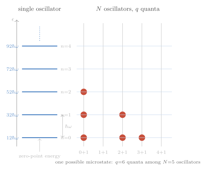
The Einstein solid (proposed by Albert Einstein in 1907) is our first and most important model system. It captures the essential physics of a crystal: \(N\) atoms, each vibrating about its equilibrium position. In quantum mechanics, a one-dimensional harmonic oscillator of angular frequency \(\omega\) has energy levels \(\epsilon_n = \hbar\omega(n + \tfrac{1}{2})\) for \(n = 0, 1, 2, \ldots\) Each atom in a three-dimensional crystal vibrates in three independent directions, so a solid of \(N\) atoms is modelled as \(3N\) quantum harmonic oscillators all sharing a common frequency \(\omega\).
Counting microstates: the stars-and-bars method
We drop the constant zero-point energy \(\tfrac{1}{2}\hbar\omega\) per oscillator (it is always present and never exchanged) and define the dimensionless energy parameter \(q = U/(\hbar\omega)\), the total number of energy quanta distributed among the \(N\) oscillators. A microstate specifies exactly how many quanta each oscillator holds; a macrostate specifies only the total \(q\) and \(N\). We want \(\Omega(N, q)\), the number of microstates corresponding to the macrostate \((N, q)\).
The counting problem maps onto a combinatorial one: in how many ways can \(q\) identical stars be arranged with \(N - 1\) identical bars in a row? Each arrangement corresponds to a distribution of quanta — the stars to the left of the first bar go to oscillator 1, those between the first and second bars go to oscillator 2, and so on. The total number of symbols is \(q + (N-1)\), and the number of distinct arrangements of \(q\) identical stars and \(N-1\) identical bars is the binomial coefficient:
\[ \Omega(N, q) = \binom{q + N - 1}{q} = \frac{(q + N - 1)!}{q!\,(N-1)!}. \]For the simplest case \(N = 3\), \(q = 2\): \(\Omega = \binom{4}{2} = 6\), agreeing with explicit enumeration. As both \(N\) and \(q\) become large — as they must for a macroscopic solid with \(N \sim 10^{23}\) — the factorials require Stirling’s approximation:
\[ \ln(n!) \approx n\ln n - n \qquad (n \gg 1), \]which leads to
\[ \ln\Omega \approx (q + N)\ln(q + N) - q\ln q - N\ln N. \]In the limit where each oscillator holds many quanta on average, \(q \gg N\), this simplifies further to \(\ln\Omega \approx N\ln(q/N) + N\), a result that will prove essential for extracting the temperature.
Chapter 8: Two Einstein Solids in Thermal Contact
The fundamental assumption
Two Einstein solids, A and B, with \(N_A\) and \(N_B\) oscillators respectively, are placed in thermal contact: they can exchange energy but the total \(q_{\text{tot}} = q_A + q_B\) is fixed. For any given split \(q_A\), the number of microstates of the combined system is
\[ \Omega_\text{tot}(q_A) = \Omega_A(N_A, q_A)\,\cdot\,\Omega_B(N_B, q_{\text{tot}} - q_A). \]The fundamental assumption of statistical mechanics is that all accessible microstates are equally probable. With this assumption, the probability of observing a particular macrostate \(q_A\) is proportional to \(\Omega_\text{tot}(q_A)\) — the most probable macrostate is the one with the most microstates.
Sharpness of the peak
For a small system (\(N_A = N_B = 3\), \(q_{\text{tot}} = 6\)), the function \(\Omega_\text{tot}(q_A)\) has a gentle maximum at equal sharing \(q_A = q_B = 3\), but the peak is only a few times the value at the extremes — there is an appreciable probability of one solid hogging nearly all the energy.
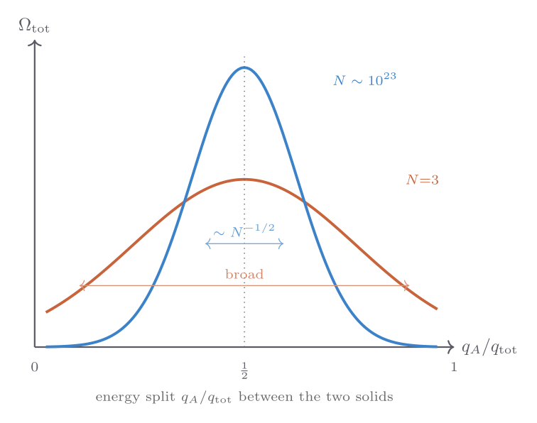
As \(N_A = N_B = N\) grows, the peak sharpens dramatically. Using Stirling’s approximation one can show that the relative width of the peak scales as \(N^{-1/2}\): for \(N = 10^{23}\), the relative fluctuation in \(q_A\) around its equilibrium value is of order \(10^{-11}\). This is the statistical basis of the second law of thermodynamics: the approach to the most probable macrostate is so overwhelmingly favoured that deviations are, for all practical purposes, impossible. What looks like an irreversible tendency — heat flowing from hot to cold, systems approaching equilibrium — is simply the system exploring its microstates and ending up in the overwhelmingly most probable macrostate.
The equal-sharing macrostate corresponds to thermal equilibrium. But why is equal-energy-per-oscillator the most probable? The multiplicity grows very steeply with energy when energy is scarce (low \(q\)), so adding energy to the solid with less energy increases the total multiplicity more than it decreases the multiplicity of the other. The system explores its microstates, and finds — overwhelmingly — that the energy distributes until neither transfer direction increases the total multiplicity. That condition defines equilibrium.
This argument makes vivid why thermal equilibrium always involves the maximisation of entropy rather than the minimisation of energy. Energy is not the relevant quantity to extremise when heat can flow freely; instead, the equilibrium condition is that the total entropy — the logarithm of the total number of accessible microstates — reaches its maximum. The tendency to maximise entropy is not an additional postulate of thermodynamics layered on top of mechanics; it is a consequence of the fundamental assumption of equal probability combined with the combinatorial fact that, for large systems, the overwhelmingly most probable macrostate has a multiplicity that dwarfs all others combined. This is why the second law, while statistical in origin, is effectively absolute for macroscopic systems: the probability of observing a spontaneous decrease in entropy over any realistic observation time is not merely small but stupendously, inconceivably small.
Chapter 9: Statistical Definition of Temperature; Two-State Systems
Temperature from entropy
The insight from Chapter 8 — that equilibrium is the state of maximum total multiplicity — motivates a precise definition. We define the entropy of a system by
\[ S = k_{\mathrm{B}}\ln\Omega, \]where \(k_{\mathrm{B}}\) is Boltzmann’s constant, included to make \(S\) an extensive quantity with units of J/K matching the classical thermodynamic entropy. The factor of \(k_{\mathrm{B}}\) is the bridge between the counting of microscopic states and the macroscopic thermal quantities defined in Part I.
With this definition, the equilibrium condition — maximum total entropy — reads
\[ \frac{\partial S_A}{\partial U_A} = \frac{\partial S_B}{\partial U_B}. \]We define the temperature as the quantity that is equal between two systems in thermal equilibrium:
\[ \frac{1}{T} \equiv \left(\frac{\partial S}{\partial U}\right)_{V, N}. \]This is the microscopic definition of temperature. It coincides exactly with the ideal-gas-thermometer definition introduced in Part I — one can verify this by computing \(\partial S/\partial U\) for the Sackur-Tetrode entropy of an ideal gas (Chapter 10). A system with steeply rising \(\Omega(U)\) — one that gains many microstates for each unit of energy added — has low temperature. A system with slowly rising \(\Omega(U)\) has high temperature. If system A has higher temperature than B, meaning \(\partial S_A/\partial U_A < \partial S_B/\partial U_B\), then transferring energy from A to B increases the total entropy — the spontaneous direction of heat flow is from hot to cold, as expected.
For the Einstein solid in the large-\(q\) limit, \(S \approx Nk_{\mathrm{B}}\ln(q/N) + \text{const}\), and \(\partial S/\partial U = (Nk_{\mathrm{B}}/\hbar\omega)\cdot(1/q)\). Since \(q = U/(\hbar\omega)\), this is \(\partial S/\partial U = Nk_{\mathrm{B}}/U\). Setting this equal to \(1/T\) gives
\[ U = Nk_{\mathrm{B}}T, \]predicting heat capacity \(C_V = Nk_{\mathrm{B}}\). This is the Dulong-Petit law, confirmed experimentally for most metals near room temperature. At low temperatures the quantum discreteness of the energy levels matters and the classical equipartition value overestimates the heat capacity — Einstein’s 1907 correction correctly predicted the falling heat capacity, a landmark early success of quantum theory.
Two-state systems and the Schottky anomaly
A simpler model than the Einstein solid is a system of \(N\) non-interacting spin-\(\tfrac{1}{2}\) particles in a magnetic field, each of which can be in one of two states — spin up (energy \(-\mu B\)) or spin down (energy \(+\mu B\)). With \(N_\uparrow\) particles in the lower-energy state and \(N_\downarrow = N - N_\uparrow\) in the upper,
\[ \Omega = \binom{N}{N_\uparrow}, \qquad U = N_\downarrow \cdot 2\mu B - N\mu B. \]Applying the entropy definition and \(1/T = \partial S/\partial U\) yields
\[ C_V = Nk_{\mathrm{B}}\left(\frac{\epsilon}{k_{\mathrm{B}}T}\right)^2 \frac{e^{\epsilon/k_{\mathrm{B}}T}}{\left(e^{\epsilon/k_{\mathrm{B}}T} + 1\right)^2}, \]where \(\epsilon = 2\mu B\). This function — known as the Schottky anomaly — vanishes at both \(T \to 0\) (insufficient thermal energy to excite the upper state) and \(T \to \infty\) (both states equally populated, no further energy can be stored), with a broad maximum at \(T \approx 0.42\,\epsilon/k_{\mathrm{B}}\).
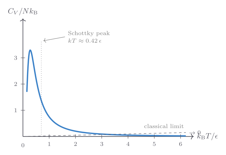
A Schottky anomaly in the specific heat of a material is a diagnostic signature of a two-level system. It appears in magnetic materials (where it is driven by the magnetic-field splitting of spin states), in glasses (where tunnelling two-level systems give a characteristic low-temperature heat capacity), and in some molecular crystals (where quantum rotational tunnelling provides the two-level structure).
The two-state system also illustrates negative absolute temperature, a subtle but real phenomenon. For a spin system, the entropy \(S(U)\) has a maximum at \(U = 0\) (equal populations, maximum disorder), so \(\partial S/\partial U = 0\) and \(1/T = 0\), corresponding to \(T = \pm\infty\). If extra energy is added beyond this point — achieved in magnetic systems by rapid field reversal — the population inversion makes \(\partial S/\partial U < 0\) and \(T < 0\). Negative-temperature states are “hotter” than any positive temperature: heat flows from a negative-temperature body to any body at finite positive temperature. They arise only in systems with a bounded energy spectrum (a maximum possible energy), which includes nuclear and electronic spin systems but not gases or phonons. The concept does not violate the laws of thermodynamics but does require a careful re-examination of the statistical foundation.
Chapter 10: The Monatomic Ideal Gas and the Sackur-Tetrode Equation
Why the ideal gas needs new tools
The Einstein solid lives in a space without volume: it has no concept of pressure. To generalise the microscopic framework to a gas, we must count states for particles that can move freely in a three-dimensional volume. This requires quantum mechanics — specifically, the quantisation of a particle in a box — and a careful treatment of the indistinguishability of identical particles.
Counting states in momentum space
A single particle of mass \(m\) confined to a cubical box of side \(L\) has allowed momenta
\[ \mathbf{p} = \frac{\pi\hbar}{L}(n_x, n_y, n_z), \qquad n_i = 1, 2, 3, \ldots \]Each point in the positive octant of momentum space occupies a “cell” of volume \((\pi\hbar/L)^3\). The number of states with magnitude of momentum less than \(p_{\max} = \sqrt{2mU}\) is proportional to the volume of a \(3N\)-dimensional hypersphere (for \(N\) particles) of radius \(\sqrt{2mU}\). Using the formula for the volume of a \(d\)-dimensional hypersphere,
\[ \mathcal{V}_d(R) = \frac{\pi^{d/2}}{\Gamma(d/2 + 1)}R^d, \]one obtains (for \(d = 3N\)) the number of states with energy less than \(U\). Differentiating gives the density of states, and multiplying by a small energy window \(\delta U\) gives \(\Omega\).
The crucial step — required to avoid the Gibbs paradox — is to divide by \(N!\) to account for the indistinguishability of identical particles. Without this factor, mixing two samples of the same gas at the same temperature and pressure would appear to increase the entropy, which is physically wrong (entropy of mixing is zero for identical gases). The Gibbs paradox was paradoxical to 19th-century physicists because classical mechanics assumes particles have identity; quantum mechanics resolves it by making identical particles truly indistinguishable.
The Sackur-Tetrode equation
After these steps, the entropy of a monatomic ideal gas of \(N\) atoms in volume \(V\) with total energy \(U\) is the Sackur-Tetrode equation (1912):
\[ S = Nk_{\mathrm{B}}\left[\ln\!\left(\frac{V}{N}\left(\frac{4\pi m U}{3Nh^2}\right)^{3/2}\right) + \frac{5}{2}\right]. \]This is an exact, closed-form expression for the entropy of a quantum ideal gas valid in the classical (high-temperature) limit. Several checks confirm its correctness.
Temperature recovery: computing \(1/T = (\partial S/\partial U)_V\) gives \(U = \tfrac{3}{2}Nk_{\mathrm{B}}T\), the familiar monatomic ideal gas energy.
Pressure recovery: computing \(P/T = (\partial S/\partial V)_U\) gives \(P = Nk_{\mathrm{B}}T/V\), the ideal gas law.
Heat capacity: \(C_V = (\partial U/\partial T)_V = \tfrac{3}{2}Nk_{\mathrm{B}}\), matching experiment for noble gases.
Entropy of mixing: computing the entropy change when two different gases mix at equal volumes and temperatures gives a positive value \(\Delta S = 2Nk_{\mathrm{B}}\ln 2\); computing the same for two samples of identical gas gives \(\Delta S = 0\), thanks to the \(N!\) factor. The Gibbs paradox is resolved.
Adiabatic processes: holding \(S\) constant in the Sackur-Tetrode equation while varying \(V\) recovers \(TV^{\gamma-1} = \text{const}\) with \(\gamma = 5/3\), consistent with the macroscopic adiabat relation derived in Chapter 3.
The Sackur-Tetrode equation also reveals that entropy decreases as temperature approaches zero — consistent with the third law, which asserts that \(S \to 0\) at absolute zero for a perfect crystal. It also shows that entropy diverges logarithmically as \(T \to 0\), signalling the breakdown of the classical (high-temperature) approximation: quantum corrections become essential at low temperatures, and a proper treatment requires Bose-Einstein or Fermi-Dirac statistics (Chapter 23).
Explicit derivation: the hypersphere volume substitution
The derivation of the Sackur-Tetrode equation requires counting the number of quantum states with total energy at most \(U\) for \(N\) non-interacting particles in a cubical box of side \(L\). Each particle \(i\) has three quantum numbers \((n_{ix}, n_{iy}, n_{iz})\), each a positive integer, with single-particle energy \(\epsilon_i = (\hbar^2\pi^2/2mL^2)(n_{ix}^2 + n_{iy}^2 + n_{iz}^2)\). The total energy constraint is
\[ \sum_{i=1}^N (n_{ix}^2 + n_{iy}^2 + n_{iz}^2) \leq \frac{2mUL^2}{\hbar^2\pi^2} \equiv R^2, \]which is the interior of a \(3N\)-dimensional hypersphere of radius \(R = L\sqrt{2mU}/(\hbar\pi)\) in the \(3N\)-dimensional space of positive integers. Since only the positive-integer octant is physical, the number of lattice points inside this region is approximately \(2^{-3N}\) of the total hypersphere volume (one out of \(2^{3N}\) equal orthants), plus a small correction from surface states that is negligible for large \(N\). The volume of the \(d = 3N\) dimensional hypersphere of radius \(R\) is
\[ \mathcal{V}_{3N}(R) = \frac{\pi^{3N/2}}{\Gamma(3N/2 + 1)}\,R^{3N}. \]Substituting \(R = L(2mU)^{1/2}/(\hbar\pi)\) and using \(V = L^3\), one obtains the number of states \(\Phi(N, V, U)\) with energy at most \(U\). The multiplicity \(\Omega\) for a thin energy shell of width \(\delta U\) is \(\Omega = (d\Phi/dU)\delta U\). After dividing by \(N!\) for indistinguishability and using Stirling’s approximation for \(\Gamma(3N/2 + 1) \approx (3N/2)!\), the entropy \(S = k_{\mathrm{B}}\ln\Omega\) simplifies to the Sackur-Tetrode form. The factor \(\delta U\) appears only in the additive constant inside the logarithm and drops out when derivatives of \(S\) are taken to extract physical predictions.
Comparison with the Einstein solid and the Gibbs factor
The Sackur-Tetrode entropy differs from that of the Einstein solid in a fundamental structural way. For the Einstein solid, the multiplicity \(\Omega(N, q) = \binom{q+N-1}{q}\) is purely combinatorial and purely depends on the number of quanta and oscillators — volume plays no role. The ideal gas entropy explicitly depends on volume through \(\ln(V/N)\), reflecting the fact that the gas can sample a larger region of phase space when confined to a larger volume. This is why the ideal gas law \(P = Nk_{\mathrm{B}}T/V\) follows from \(P/T = (\partial S/\partial V)_U\) — pressure is a direct consequence of the entropy’s logarithmic volume dependence.
The \(1/N!\) Gibbs factor is quantitatively important. Without it, the entropy would be \(S_\text{wrong} = Nk_{\mathrm{B}}\ln V + \ldots\) rather than \(Nk_{\mathrm{B}}\ln(V/N) + \ldots\). The wrong formula gives \(S_\text{wrong} \propto N\ln V\), which is not extensive: doubling \(N\) and \(V\) simultaneously would give \(2N\ln(2V) = 2S + 2Nk_{\mathrm{B}}\ln 2\) rather than \(2S\). Only with the \(1/N!\) does the entropy scale correctly as an extensive quantity. The \(N!\) factor changes the logarithm of the partition function from \(\ln V^N\) to \(\ln(V^N/N!)\), and via Stirling’s approximation: \(\ln(V^N/N!) \approx N\ln(V/N) + N\), the crucial \(N\) appears in the denominator of the logarithm, ensuring extensivity. Physically, this factor reflects the fact that quantum mechanics forbids assigning persistent identities to identical particles: a configuration of \(N\) ideal gas atoms is fully described by the occupation numbers of single-particle states, not by labelling which atom is in which state.
Chapter 11: The Boltzmann Distribution and the Canonical Partition Function
Beyond fixed energy: contact with a reservoir
The microcanonical ensemble (fixed \(U\), \(V\), \(N\)) underlying the Einstein solid analysis is elegant but restrictive. Most real systems are in contact with a heat reservoir — a large body at fixed temperature \(T\) with which they can exchange energy. The relevant ensemble is the canonical ensemble, where \(T\), \(V\), and \(N\) are fixed rather than \(U\).
Consider a small system \(s\) in contact with a large reservoir \(r\) at temperature \(T\). The total energy \(U_\text{tot} = \epsilon_s + U_r\) is conserved. By the fundamental assumption, the probability that the system is in a specific microstate with energy \(\epsilon_s\) is proportional to the multiplicity of the reservoir when it has energy \(U_\text{tot} - \epsilon_s\):
\[ P(\epsilon_s) \propto \Omega_r(U_\text{tot} - \epsilon_s) = e^{S_r(U_\text{tot} - \epsilon_s)/k_{\mathrm{B}}}. \]Expanding the reservoir entropy to first order in \(\epsilon_s\) (valid because the reservoir is large):
\[ S_r(U_\text{tot} - \epsilon_s) \approx S_r(U_\text{tot}) - \frac{\epsilon_s}{T}, \]giving the Boltzmann distribution:
\[ \boxed{P(\epsilon_s) = \frac{e^{-\epsilon_s/k_{\mathrm{B}}T}}{Z}, \qquad Z \equiv \sum_j e^{-\epsilon_j/k_{\mathrm{B}}T}.} \]The sum \(Z\) over all microstates of the system is the partition function. The factor \(e^{-\epsilon/k_{\mathrm{B}}T}\) is the Boltzmann factor; higher-energy states are exponentially less probable.
The partition function and thermodynamics
The partition function encodes all thermodynamic information about the system. The mean energy is
\[ \langle U \rangle = -\frac{\partial \ln Z}{\partial \beta}, \qquad \beta \equiv \frac{1}{k_{\mathrm{B}}T}. \]The Helmholtz free energy is \(F = -k_{\mathrm{B}}T\ln Z\), and all other thermodynamic quantities follow by standard differentiation:
\[ S = -\left(\frac{\partial F}{\partial T}\right)_V, \quad P = -\left(\frac{\partial F}{\partial V}\right)_T, \quad \mu = \left(\frac{\partial F}{\partial N}\right)_{T,V}. \]For a monatomic ideal gas, the partition function factorises over particles: \(Z = z^N/N!\) where \(z = V/\lambda_\text{th}^3\) is the single-particle partition function, and \(\lambda_\text{th} = h/\sqrt{2\pi mk_{\mathrm{B}}T}\) is the thermal de Broglie wavelength. Computing \(F = -k_{\mathrm{B}}T\ln Z\) and then \(S = -(\partial F/\partial T)_V\) recovers the Sackur-Tetrode equation — a satisfying consistency check.
The classical regime corresponds to \(V/N \gg \lambda_\text{th}^3\): the mean volume per particle is much larger than the cube of the thermal de Broglie wavelength. When this condition fails, quantum statistics become essential and the classical partition function breaks down.
Mathematical framework of the partition function
The partition function \(Z(\beta, V, N) = \sum_j e^{-\beta\epsilon_j}\) encodes all thermodynamic information about a system in the canonical ensemble. The connection to the Helmholtz free energy \(F = -k_{\mathrm{B}}T\ln Z\) is the master relation from which everything else follows by differentiation.
The mean energy is obtained by differentiating with respect to \(\beta\):
\[ \langle U \rangle = -\frac{\partial \ln Z}{\partial \beta} = k_{\mathrm{B}}T^2\frac{\partial \ln Z}{\partial T}. \]The entropy is \(S = -(\partial F/\partial T)_V\):
\[ S = k_{\mathrm{B}}\ln Z + \frac{\langle U \rangle}{T} = k_{\mathrm{B}}\left(\ln Z - \beta\frac{\partial \ln Z}{\partial \beta}\right). \]The heat capacity follows as \(C_V = (\partial\langle U\rangle/\partial T)_V = k_{\mathrm{B}}\beta^2\,\partial^2\ln Z/\partial\beta^2\). It is also the energy variance divided by \((k_{\mathrm{B}}T)^2\): \(C_V = (\langle U^2\rangle - \langle U\rangle^2)/(k_{\mathrm{B}}T^2)\). This fluctuation-response relation is a special case of the fluctuation-dissipation theorem.
Worked example: two-level system
Consider a single quantum system with two levels: ground state at energy 0 and excited state at energy \(\epsilon\). The partition function is \(Z = 1 + e^{-\beta\epsilon}\). The mean energy is
\[ \langle U \rangle = -\frac{\partial\ln Z}{\partial\beta} = \frac{\epsilon\,e^{-\beta\epsilon}}{1 + e^{-\beta\epsilon}} = \frac{\epsilon}{e^{\beta\epsilon} + 1}. \]The heat capacity is
\[ C = k_{\mathrm{B}}\left(\frac{\epsilon}{k_{\mathrm{B}}T}\right)^2\frac{e^{\epsilon/k_{\mathrm{B}}T}}{(e^{\epsilon/k_{\mathrm{B}}T} + 1)^2}, \]which is the Schottky anomaly encountered in Chapter 9. The entropy is
\[ S = k_{\mathrm{B}}\ln(1 + e^{-\beta\epsilon}) + \frac{\epsilon}{T(e^{\beta\epsilon} + 1)}. \]At high temperatures \((k_{\mathrm{B}}T \gg \epsilon)\), both levels are equally populated and \(S \to k_{\mathrm{B}}\ln 2\) — the maximum entropy for a two-level system. For \(N\) independent such systems, all quantities scale by \(N\): \(\langle U\rangle_N = N\langle U\rangle\), \(C_N = NC\), \(S_N = NS\).
Worked example: harmonic oscillator from the partition function
For a quantum harmonic oscillator with energy levels \(\epsilon_n = \hbar\omega(n + 1/2)\), the partition function is \(Z = e^{-\beta\hbar\omega/2}\sum_{n=0}^\infty e^{-n\beta\hbar\omega} = e^{-\beta\hbar\omega/2}/(1 - e^{-\beta\hbar\omega})\). Taking the logarithm: \(\ln Z = -\beta\hbar\omega/2 - \ln(1 - e^{-\beta\hbar\omega})\). Differentiating with respect to \(-\beta\) gives the mean energy:
\[ \langle U \rangle = \frac{\hbar\omega}{2} + \frac{\hbar\omega}{e^{\hbar\omega/k_{\mathrm{B}}T} - 1}. \]The first term is the zero-point energy (present even at \(T = 0\)); the second is the thermal excitation. At high temperatures, \(e^x - 1 \approx x\) gives \(\langle U\rangle \approx \hbar\omega/2 + k_{\mathrm{B}}T\), and dropping the (constant) zero-point energy, \(C_V = k_{\mathrm{B}}\) per oscillator — consistent with classical equipartition. For \(N\) oscillators (Einstein solid with \(3N\) oscillators per atom), the high-temperature limit \(C_V = 3Nk_{\mathrm{B}}\) is the Dulong-Petit law.
The partition-function route to thermodynamics is superior to the microcanonical route (direct counting) when the energies are complicated or continuous. For systems with many types of excitation — electronic, vibrational, rotational, translational — one can often write \(Z = Z_\text{trans} \times Z_\text{rot} \times Z_\text{vib} \times Z_\text{elec}\) because the energies are approximately additive, and the free energy is then the sum of the free energies of each mode: \(F = F_\text{trans} + F_\text{rot} + \ldots\).
Application: the Einstein solid from the partition function
For a single quantum harmonic oscillator, \(Z = \sum_{n=0}^\infty e^{-n\beta\hbar\omega} = 1/(1 - e^{-\beta\hbar\omega})\). The mean energy is
\[ \langle \epsilon \rangle = \frac{\hbar\omega}{e^{\hbar\omega/k_{\mathrm{B}}T} - 1} + \frac{\hbar\omega}{2}. \]For \(N\) oscillators in the Einstein solid, \(\langle U \rangle = N\langle \epsilon \rangle - N\hbar\omega/2\), and the heat capacity is
\[ C_V = Nk_{\mathrm{B}}\left(\frac{\hbar\omega}{k_{\mathrm{B}}T}\right)^2 \frac{e^{\hbar\omega/k_{\mathrm{B}}T}}{\left(e^{\hbar\omega/k_{\mathrm{B}}T} - 1\right)^2}. \]At high temperatures (\(k_{\mathrm{B}}T \gg \hbar\omega\)) this reduces to \(C_V = Nk_{\mathrm{B}}\), recovering the Dulong-Petit law. At low temperatures it vanishes exponentially, resolving the classical equipartition disaster. The Debye model (Chapter 24) improves on this by allowing a distribution of oscillator frequencies, giving the observed \(T^3\) dependence of solid heat capacities at low temperature.
The Einstein model’s prediction of an exponentially vanishing heat capacity at low temperature — \(C_V \sim N k_{\mathrm{B}}(\hbar\omega/k_{\mathrm{B}}T)^2 e^{-\hbar\omega/k_{\mathrm{B}}T}\) — is qualitatively correct but quantitatively too fast compared to the observed \(T^3\) fall-off in crystalline solids. The discrepancy arises because the Einstein model assigns all oscillators the same frequency. In reality, a crystal supports lattice vibrations (phonons) with a continuous spectrum of frequencies from zero (long-wavelength acoustic modes) up to a maximum Debye frequency. The long-wavelength acoustic phonons persist down to arbitrarily low temperatures and are responsible for the \(T^3\) behaviour. Einstein’s model was nonetheless a landmark — the first demonstration that quantum theory could resolve the contradiction between classical equipartition and experimental heat-capacity data, and a proof of concept that quantum mechanics applied to macroscopic matter.
Chapter 12: Kinetic Theory — Maxwell-Boltzmann Distribution, Mean Free Path, and Transport
The Maxwell-Boltzmann speed distribution
The Boltzmann distribution applied to the translational motion of an ideal gas gives the probability that a molecule has velocity \(\mathbf{v}\). Since kinetic energy \(\epsilon = \tfrac{1}{2}mv^2\) depends only on speed in an isotropic gas, the distribution separates into three independent Gaussian factors. The Maxwell-Boltzmann speed distribution — the probability that a molecule has speed between \(v\) and \(v + dv\) — is
\[ f(v) = 4\pi n \left(\frac{m}{2\pi k_{\mathrm{B}}T}\right)^{3/2} v^2 \exp\!\left(-\frac{mv^2}{2k_{\mathrm{B}}T}\right), \]where \(n = N/V\) is the number density. The \(v^2\) factor (from the spherical shell in velocity space) shifts the peak away from zero; the Gaussian envelope cuts off the high-speed tail.
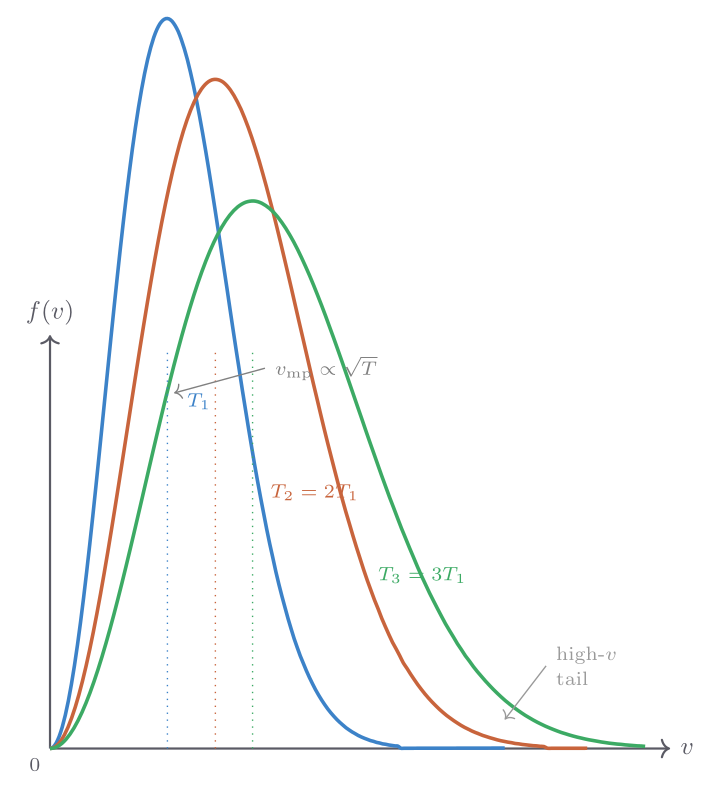
Three characteristic speeds are:
\[ v_\text{mp} = \sqrt{\frac{2k_{\mathrm{B}}T}{m}} \quad (\text{most probable}), \qquad \bar{v} = \sqrt{\frac{8k_{\mathrm{B}}T}{\pi m}} \quad (\text{mean}), \qquad v_\text{rms} = \sqrt{\frac{3k_{\mathrm{B}}T}{m}} \quad (\text{root-mean-square}). \]Note \(v_\text{mp} < \bar{v} < v_\text{rms}\), all proportional to \(\sqrt{T/m}\). The distribution broadens and its peak shifts to higher speeds as temperature increases. At any temperature, there is a non-negligible fraction of molecules with speeds several times the mean — the high-speed tail is crucial for chemical reactions (only the fastest molecules overcome activation-energy barriers) and for atmospheric escape (light molecules like hydrogen whose thermal speed exceeds escape velocity slowly bleed off into space).
Mean free path
Between collisions, a molecule travels in a straight line. The mean free path \(\lambda\) is the average distance covered between successive collisions.
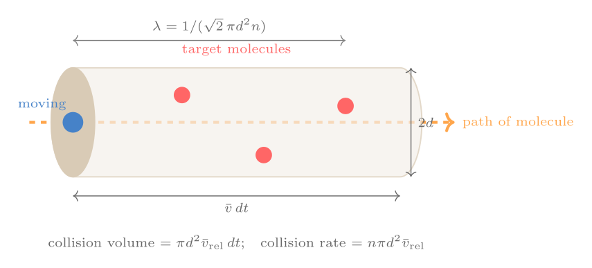
Consider a molecule of diameter \(d\) moving with mean speed \(\bar{v}\) through a gas of stationary molecules. In time \(dt\) it sweeps out a cylinder of volume \(\pi d^2 \bar{v}\,dt\). Any molecule whose centre falls inside this cylinder will be struck. The number of such molecules is \(n\pi d^2 \bar{v}\,dt\), so the collision rate is \(\bar{v}/\lambda = n\pi d^2 \bar{v}_\text{rel}\), where the relative velocity \(\bar{v}_\text{rel} = \sqrt{2}\bar{v}\) accounts for the motion of the target molecules. Hence
\[ \lambda = \frac{1}{\sqrt{2}\,\pi d^2\,n}. \]At atmospheric pressure, air molecules have \(d \approx 3.7 \times 10^{-10}\ \text{m}\) and \(n \approx 2.7 \times 10^{25}\ \text{m}^{-3}\), giving \(\lambda \approx 68\ \text{nm}\) — about 200 molecular diameters. This is why a gas behaves as a continuous fluid on macroscopic scales yet exhibits discrete molecular behaviour at the nanoscale.
Transport coefficients
The same kinetic-theory argument that gives \(\kappa_\text{th} \propto \bar{v}\lambda C_V/V\) yields analogous expressions for viscosity and diffusion. All three transport coefficients have the characteristic \(\sqrt{T}\) temperature dependence (from \(\bar{v} \propto \sqrt{T}\)) and are independent of pressure (since \(\lambda \propto 1/n\) cancels the \(n\) in \(n\bar{v}\)). This pressure-independence, predicted theoretically and confirmed by Maxwell himself, seemed deeply counterintuitive: a more dilute gas is just as viscous as a dense one, because the longer mean free path exactly compensates for fewer molecules. The viscosity of a gas increasing with temperature (unlike liquids, which become less viscous when heated) is another testament to the kinetic picture — faster molecules carry more momentum across a velocity gradient.
In a liquid, viscosity is governed by the frequency with which molecules hop between positions in the local structure — an activated process with a barrier height \(\Delta E\). The viscosity of a liquid therefore decreases approximately as \(\eta \sim e^{\Delta E/k_{\mathrm{B}}T}\) (Arrhenius form), because higher temperature gives molecules more energy to overcome intermolecular barriers. This opposite temperature dependence relative to gases is a macroscopic signal of the fundamentally different mechanisms of momentum transport in the two phases — cooperative rearrangement in liquids versus free-flight mean-free-path transport in gases.
The Knudsen number \(\text{Kn} = \lambda/L\) (ratio of mean free path to system size \(L\)) determines whether a gas is in the viscous regime (Kn \(\ll 1\), Navier-Stokes equations apply) or the molecular-flow regime (Kn \(\gg 1\), individual molecule dynamics matter). At atmospheric pressure, \(\lambda \approx 68\ \text{nm}\) and most engineering applications have \(L \gg \lambda\). In vacuum systems and microelectronics, however, the Knudsen number can reach unity or beyond, requiring a kinetic-theory description rather than fluid mechanics.
Part III: The Second Law in Macroscopic Form
Chapter 13: Entropy, Heat Flow, and the Second Law
Heat and entropy
In a quasi-static process, the first law takes the form
\[ dU = T\,dS - P\,dV, \]where \(T\,dS\) is the heat flowing in and \(-P\,dV\) is the work done on the system. Rearranging gives the fundamental thermodynamic relation between entropy change and heat flow:
\[ dS = \frac{\delta Q}{T} \quad \text{(quasi-static)}. \]This is not just a definition — it connects the statistical entropy \(S = k_{\mathrm{B}}\ln\Omega\) to the classical thermodynamic quantity \(Q/T\). The connection can be verified for any quasi-static process on a system whose entropy we have calculated microscopically.
As a concrete example, consider melting ice. At 273 K the latent heat of fusion is \(6010\ \text{J mol}^{-1}\). Adding this heat reversibly increases the entropy by \(\Delta S = Q/T = 6010/273 \approx 22\ \text{J mol}^{-1}\text{K}^{-1}\). The increase makes sense microscopically: water molecules in the liquid have far more positional freedom than those locked in the crystal lattice — the multiplicity of accessible states is vastly higher.
Now consider heat flowing spontaneously from a hot reservoir at temperature \(T_h\) to a cold one at \(T_c\). The hot reservoir loses entropy \(-Q/T_h\) while the cold reservoir gains \(+Q/T_c\). The total entropy change is
\[ \Delta S_\text{total} = Q\left(\frac{1}{T_c} - \frac{1}{T_h}\right) > 0 \qquad (T_h > T_c,\; Q > 0). \]Total entropy increases — in agreement with the microscopic picture that the final macrostate (energy shared) has more microstates than the initial one (energy concentrated).
The second law
The experimental observations about heat flow, mixing, and free expansion can all be subsumed in a single statement. In the language introduced by Max Planck:
A reversible process is one executed quasi-statically with no dissipation — an idealisation never perfectly achieved in practice. All real processes are irreversible to some degree.
The second law is statistical, not absolute. For a system of \(N\) particles, a fluctuation that transiently decreases entropy by an amount \(\Delta S\) has probability \(\sim e^{-\Delta S/k_{\mathrm{B}}}\). For macroscopic decreases (\(\Delta S \sim Nk_{\mathrm{B}}\)) this is fantastically small — roughly \(e^{-10^{23}}\). In practice the second law is absolute for any macroscopic system; violations would require us to observe the system for times vastly longer than the age of the universe. Maxwell’s demon, a hypothetical creature that could sort molecules and thereby decrease entropy without doing work, is thwarted by information theory: the demon must acquire information about molecular states, and erasing that information (as Landauer showed) dissipates at least \(k_{\mathrm{B}}T\ln 2\) per bit — enough to keep the total entropy balance non-negative.
Entropy as a state function
A central but sometimes under-emphasised fact is that entropy, despite being defined through counting microstates (or through \(dS = \delta Q/T\) for quasi-static processes), is a state function: its value depends only on the current thermodynamic state \((T, P, N)\), not on the history of the system. This can be verified for any system whose equation of state is known.
For an ideal gas, the fundamental relation \(dU = T\,dS - P\,dV\) can be rearranged as \(dS = C_V\,dT/T + (Nk_{\mathrm{B}}/V)\,dV\). Integrating between two states \((T_1, V_1)\) and \((T_2, V_2)\):
\[ \Delta S = C_V\ln\frac{T_2}{T_1} + Nk_{\mathrm{B}}\ln\frac{V_2}{V_1}. \]The result depends only on the endpoints, confirming that \(S\) is a state function. If one takes a path via isothermal expansion (at \(T_1\) from \(V_1\) to \(V_2\)) followed by isochoric heating (at \(V_2\) from \(T_1\) to \(T_2\)), the contributions add to exactly the same total. No matter which sequence of quasi-static steps is used, the entropy difference between two equilibrium states is unique — this is precisely what distinguishes entropy from \(Q\) and \(W\), which are path-dependent.
The Kelvin and Clausius statements of the second law
The second law has several equivalent formulations. The Kelvin statement asserts: it is impossible to construct a device that operates in a cycle and produces no effect other than the transfer of heat from a single reservoir to work. In other words, a perfect heat engine (converting all absorbed heat to work with no exhaust) is impossible. The Clausius statement asserts: it is impossible to construct a device that operates in a cycle and produces no effect other than the transfer of heat from a cold body to a hot body. In other words, a perfect refrigerator (pumping heat from cold to hot with no work input) is impossible.
These statements look different but are logically equivalent: assuming the violation of either one leads directly to the violation of the other. To see this, suppose a device transfers heat \(Q_c\) from a cold reservoir to a hot one without work input (violating Clausius). Combine it with a Carnot engine absorbing \(Q_h > Q_c\) from the hot reservoir, doing work \(W = Q_h - Q_c\), and discarding \(Q_c\) to the cold reservoir. The net result: the cold-reservoir contributions cancel, and the combined device converts \(Q_h - Q_c\) of heat from the hot reservoir entirely into work — a Kelvin violation.
Entropy production in irreversible processes
For any real (irreversible) process, the Clausius inequality states \(dS \geq \delta Q/T\), with equality holding only for reversible processes. The entropy production \(\sigma = dS - \delta Q/T \geq 0\) quantifies the irreversibility. It is zero for ideal quasi-static processes and positive for everything real: friction, heat conduction across a finite temperature difference, free expansion, chemical reactions proceeding to equilibrium.
As a concrete example, consider 1 mole of ideal gas expanding freely into vacuum, doubling its volume (Joule expansion). Since \(\delta Q = 0\) and \(W = 0\), we have \(\Delta U = 0\) and thus \(\Delta T = 0\). The entropy change is \(\Delta S = Nk_{\mathrm{B}}\ln 2 = R\ln 2 \approx 5.76\ \text{J K}^{-1}\). This entropy was produced entirely internally — the process is irreversible. To restore the original state, an isothermal compression of the gas must be performed, requiring work \(W = RT\ln 2\) from an external agent and transferring heat \(Q = RT\ln 2\) to a reservoir, increasing the reservoir’s entropy by exactly \(R\ln 2\) and restoring the gas entropy to its original value. The entropy of the universe increases by \(R\ln 2\) in the free expansion and cannot be reclaimed without increasing the total entropy of the universe by at least as much again.
Chapter 14: Entropy of Mixing and the Gibbs Paradox
Mixing two different gases
When two different ideal gases (say, helium at density \(n\) in volume \(V\), and argon at density \(n\) in an equal volume \(V\)) are allowed to mix by removing a partition, each gas expands into the full volume \(2V\). Since the gases are ideal (no interactions), each behaves as if the other were absent. The entropy change of each component is, from the Sackur-Tetrode equation,
\[ \Delta S_\text{He} = \Delta S_\text{Ar} = Nk_{\mathrm{B}}\ln 2, \]giving \(\Delta S_\text{mix} = 2Nk_{\mathrm{B}}\ln 2 > 0\). This entropy of mixing is irreversible: the gases do not spontaneously un-mix. No work is required to mix them — entropy drives the process.
For a mixture of \(k\) different gases with mole fractions \(x_i = N_i/N\), the entropy of mixing per molecule is
\[ \frac{\Delta S_\text{mix}}{N} = -k_{\mathrm{B}}\sum_i x_i \ln x_i \geq 0, \]with equality only when the mixture is pure (\(x_i = 1\) for one component). This formula is fundamental in chemistry (Raoult’s law, colligative properties), biology (osmotic pressure), and information theory (where the same expression defines the Shannon entropy of a probability distribution, up to a constant).
The Gibbs paradox and indistinguishability
Now consider the mixing of identical gases — helium on both sides. The partition is removed; nothing changes. The entropy should not change. Yet if we forget that the molecules are identical and apply the mixing formula blindly, we predict an entropy increase of \(2Nk_{\mathrm{B}}\ln 2\) — the same as for two different gases. This contradiction is the Gibbs paradox.
The resolution requires the \(1/N!\) factor in the partition function (Chapter 10). When identical molecules are truly indistinguishable, swapping them does not create a new microstate. With the \(1/N!\) factor, the Sackur-Tetrode equation gives \(\Delta S = 0\) when identical gases mix — the paradox disappears. Gibbs struggled to explain this in the 1870s without quantum mechanics; the complete resolution came only with quantum theory, which made indistinguishability a fundamental postulate rather than an ad hoc counting rule.
Detailed derivation of the entropy of mixing
The Sackur-Tetrode equation for a pure gas of \(N\) atoms in volume \(V\) at temperature \(T\) (i.e., at energy \(U = \tfrac{3}{2}Nk_{\mathrm{B}}T\)) takes the form \(S = Nk_{\mathrm{B}}[f(T) + \ln(V/N)]\), where \(f(T)\) depends only on temperature and not on volume or number of particles. When helium (species 1, \(N_1\) atoms) and argon (species 2, \(N_2\) atoms), both at temperature \(T\), each initially occupy volume \(V\), they are separated by a partition. After the partition is removed and equilibrium is reached, each species occupies the total volume \(V_1 + V_2 = 2V\) (taking \(N_1 = N_2 = N\) and \(V_1 = V_2 = V\) for simplicity). The entropy of species 1 after mixing is
\[ S_1^\text{after} = Nk_{\mathrm{B}}\left[f_1(T) + \ln\frac{2V}{N}\right] = Nk_{\mathrm{B}}\left[f_1(T) + \ln\frac{V}{N} + \ln 2\right] = S_1^\text{before} + Nk_{\mathrm{B}}\ln 2, \]and likewise for species 2. The total entropy of mixing is
\[ \Delta S_\text{mix} = 2Nk_{\mathrm{B}}\ln 2, \]which is positive and corresponds to each gas exploring twice the available volume. For a general mixture of \(k\) components with mole fractions \(x_i = N_i/N_\text{tot}\), each species \(i\) expands from volume \(x_i V_\text{tot}\) to \(V_\text{tot}\), giving \(\Delta S_i = N_i k_{\mathrm{B}}\ln(1/x_i)\), and the total is
\[ \Delta S_\text{mix} = -Nk_{\mathrm{B}}\sum_i x_i\ln x_i. \]This formula, identical in structure to the Shannon entropy of information theory (with \(k_{\mathrm{B}}\) replacing Boltzmann’s constant and \(x_i\) as probabilities), is the foundation of Raoult’s law in solution chemistry, the chemical potential of an ideal mixture, and the van’t Hoff equation for osmotic pressure.
The Gibbs paradox resolution and the role of \(1/N!\) in Boltzmann counting
The Gibbs paradox makes the indistinguishability requirement vivid. When identical gases mix, the physical state does not change — the entropy should remain constant. Applying the Sackur-Tetrode formula correctly, with the \(1/N!\) factor:
\[ S^\text{after} = 2N k_{\mathrm{B}}\left[f(T) + \ln\frac{2V}{2N}\right] = 2Nk_{\mathrm{B}}\left[f(T) + \ln\frac{V}{N}\right] = 2 \times S_\text{each\;before}, \]giving \(\Delta S = 0\), as required. Without the \(1/N!\) factor, the \(\ln(V/N)\) would become \(\ln V\), and mixing identical gases would spuriously produce \(\Delta S = 2Nk_{\mathrm{B}}\ln 2\).
The \(1/N!\) factor enters the partition function because, for identical quantum particles, the partition function for \(N\) non-interacting particles is \(Z_N = z^N / N!\) rather than \(z^N\). Here \(z\) is the single-particle partition function. The \(N!\) accounts for the \(N!\) permutations of \(N\) identical particles among their states that give the same physical configuration. Physically: if we label classical identical particles 1 through \(N\) and swap any two, we do not create a new microstate — the physical state is unchanged. Failing to divide by \(N!\) would count each physical microstate \(N!\) times, vastly overcounting and producing an extensive inconsistency. This over-counting error was present in all of classical statistical mechanics until Gibbs, who introduced the \(1/N!\) on phenomenological grounds; quantum mechanics later provided its theoretical justification by defining identical particles as fundamentally without individual identity.
Chapter 15: Cyclic Heat Engines
The general heat-engine problem
A heat engine is a device that operates in a cycle, absorbing heat \(Q_h\) from a hot reservoir at temperature \(T_h\), performing work \(W_\text{out}\), and discarding heat \(Q_c\) to a cold reservoir at \(T_c\). By the first law over one complete cycle (\(\Delta U_\text{engine} = 0\)):
\[ Q_h = W_\text{out} + Q_c. \]The efficiency is \(\eta = W_\text{out}/Q_h = 1 - Q_c/Q_h\).
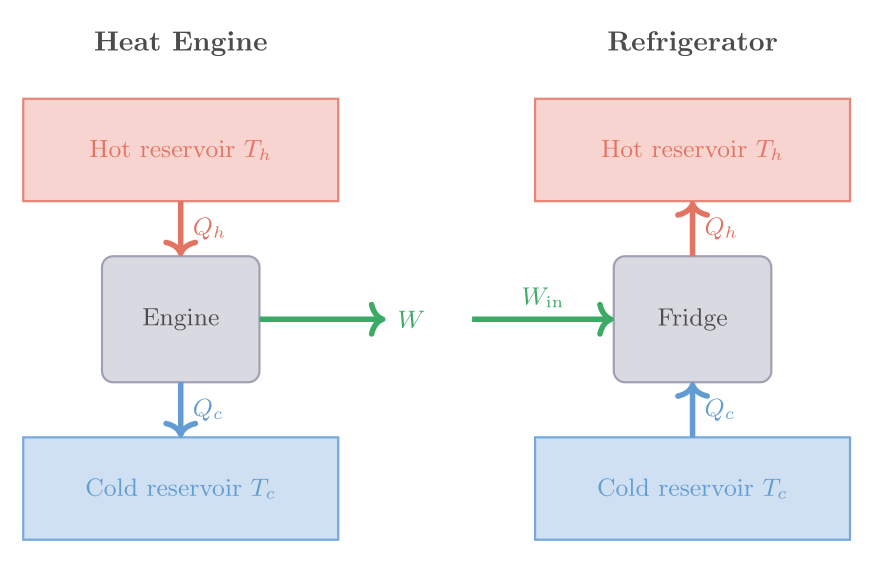
The second law constrains \(\eta\). Over one cycle, the total entropy change of the universe (engine + reservoirs) must be non-negative:
\[ \Delta S_\text{universe} = -\frac{Q_h}{T_h} + \frac{Q_c}{T_c} \geq 0. \]This gives \(Q_c/Q_h \geq T_c/T_h\), and hence
\[ \eta \leq 1 - \frac{T_c}{T_h} \equiv \eta_\text{Carnot}. \]The Carnot efficiency \(\eta_\text{Carnot}\) is the maximum efficiency of any heat engine operating between temperatures \(T_h\) and \(T_c\). Equality holds only for reversible engines (\(\Delta S_\text{universe} = 0\)).
The Carnot cycle
The Carnot cycle achieves the maximum efficiency. It consists of four quasi-static steps:
- Isothermal expansion at \(T_h\): the gas absorbs \(Q_h\).
- Adiabatic expansion: the gas cools from \(T_h\) to \(T_c\).
- Isothermal compression at \(T_c\): the gas releases \(Q_c\).
- Adiabatic compression: the gas warms from \(T_c\) to \(T_h\).
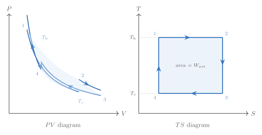
On a \(T\)–\(S\) diagram the Carnot cycle is a rectangle: the isothermal steps are horizontal, the adiabatic steps (constant \(S\)) are vertical. The area of the rectangle equals the net work done. This geometric simplicity makes the \(T\)–\(S\) diagram the natural representation for heat-engine analysis.
For an ideal gas working substance, the heat inputs and outputs can be computed from the isothermal work: \(Q_h = Nk_{\mathrm{B}}T_h\ln(V_B/V_A)\), \(Q_c = Nk_{\mathrm{B}}T_c\ln(V_C/V_D)\). Using the adiabat relations one can show \(V_B/V_A = V_C/V_D\), so \(Q_c/Q_h = T_c/T_h\) exactly — confirming Carnot efficiency.
The Carnot engine is reversible and therefore maximally efficient, but it is also infinitely slow (quasi-static). Real engines must run at finite power, and there is a fundamental trade-off between efficiency and power. Curzon and Ahlborn (1975) showed that the efficiency at maximum power of an endoreversible engine — one where all irreversibility occurs in the heat-transfer steps — is \(\eta_\text{CA} = 1 - \sqrt{T_c/T_h}\), which lies between \(\eta_\text{Carnot}\) and zero and agrees surprisingly well with the design efficiencies of real power stations.
The Carnot cycle on a \(T\)–\(S\) diagram is a rectangle with sides at \(T = T_h\), \(T = T_c\), and \(S = S_1\), \(S = S_2\). The net work per cycle is the area of this rectangle: \(W = (T_h - T_c)(S_2 - S_1) = (T_h - T_c)\,\Delta S\). The heat absorbed from the hot reservoir is the area under the top horizontal segment: \(Q_h = T_h\,\Delta S\). The ratio \(W/Q_h = (T_h - T_c)/T_h = \eta_\text{Carnot}\), as expected. This geometric interpretation of the \(T\)–\(S\) diagram makes the Carnot efficiency transparent: work is the difference between the heat rectangles at the two temperatures, and maximising efficiency means maximising the ratio of the work area to the heat-input area — which requires the cycle to spend as much time as possible at the highest available temperature and as little as possible at the lowest.
The Otto cycle
The Otto cycle is the idealised model of a spark-ignition gasoline engine. Its four steps on a \(PV\) diagram are:
- Adiabatic compression: \(V_A \to V_B\) (compression ratio \(r = V_A/V_B\)).
- Constant-volume heat addition (simulating ignition): pressure rises at fixed volume.
- Adiabatic expansion: \(V_B \to V_A\) (power stroke).
- Constant-volume heat rejection (exhaust).
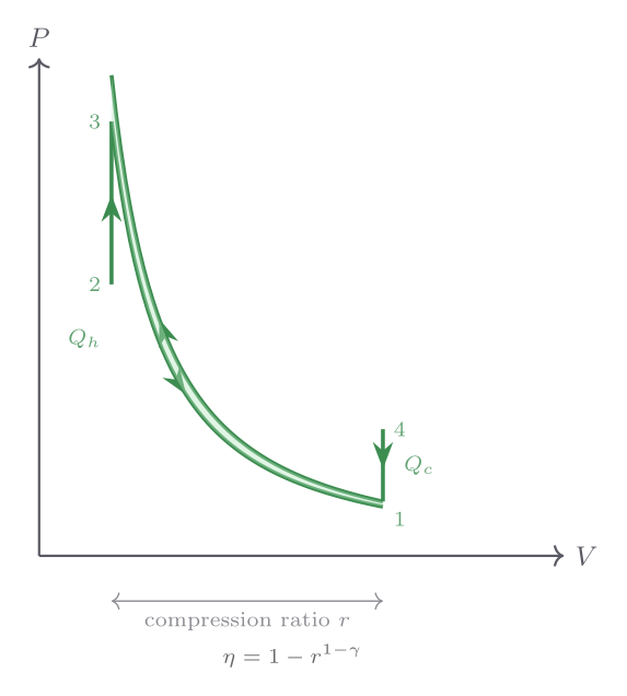
The efficiency is
\[ \eta_\text{Otto} = 1 - \frac{1}{r^{\gamma - 1}}. \]For \(\gamma = 1.4\) (air) and a compression ratio \(r = 10\) (typical for gasoline engines), \(\eta_\text{Otto} = 1 - 10^{-0.4} \approx 0.60\). Actual gasoline engines achieve 25–35% because of friction, heat loss, and combustion irreversibility.
The Diesel cycle
The Diesel cycle models a compression-ignition engine. The key difference from Otto is that heat addition occurs at constant pressure (as fuel is injected and burns progressively) rather than constant volume. The compression ratio is typically \(r = 15–22\) — much higher than in gasoline engines — because no fuel is present during compression, eliminating the risk of premature ignition. The adiabatic compression to these high ratios raises the air temperature to \(\sim 700–900\) °C, sufficient for spontaneous ignition of injected diesel fuel.
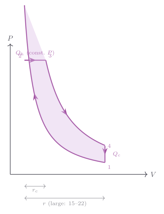
With cutoff ratio \(r_c = V_C/V_B\) (ratio of volume after and before fuel injection), the efficiency is
\[ \eta_\text{Diesel} = 1 - \frac{1}{r^{\gamma-1}}\cdot\frac{r_c^\gamma - 1}{\gamma(r_c - 1)}. \]Because \(r_c > 1\) always, the bracketed fraction exceeds 1, making the Diesel efficiency lower than Otto at the same compression ratio. But diesel engines use much higher compression ratios, and in practice they achieve 40–45% efficiency — higher than gasoline engines. Modern turbocharged diesel engines used in trucks and ships can approach 50%.
The Stirling cycle
The Stirling cycle (1816, Robert Stirling) consists of two isothermal steps connected by two constant-volume (isochoric) steps. What makes it special is the regenerator: thermal energy rejected during the hot-to-cold isochoric step is stored and returned to the gas during the cold-to-hot step, so the only heat exchanges with external reservoirs occur during the isothermal steps. The efficiency then equals the Carnot efficiency — the Stirling cycle is one of the few practically realisable cycles that achieves Carnot efficiency in principle.
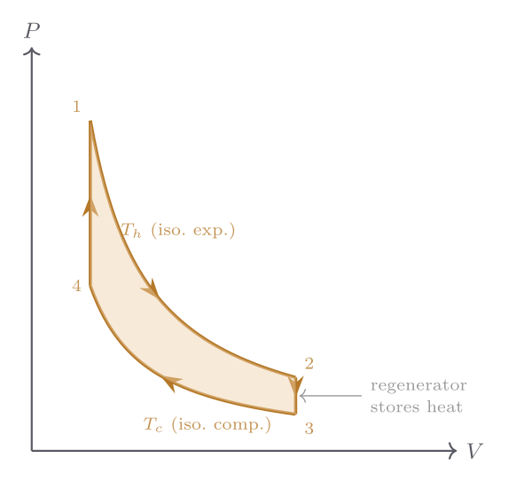
Practical Stirling engines — compact, quiet, and amenable to external combustion or solar heating — are used in space power systems and cryocoolers. The Stirling-cycle refrigerator (running the cycle in reverse) is the standard technology for cooling infrared detectors to liquid-helium temperatures in space applications.
Chapter 16: Refrigeration, Throttling, and the Joule-Thomson Coefficient
Refrigerators and heat pumps
A refrigerator is a heat engine run in reverse: work is supplied to pump heat from a cold reservoir to a hot one. Over one cycle, \(W_\text{in} + Q_c = Q_h\). The coefficient of performance (COP) is
\[ \text{COP}_\text{refrigerator} = \frac{Q_c}{W_\text{in}} = \frac{T_c}{T_h - T_c} \quad (\text{reversible limit}). \]A heat pump heats a building by extracting heat from the cold outdoors; its COP is \(Q_h/W_\text{in} = T_h/(T_h - T_c)\). For outdoor temperature \(-5\) °C and indoor \(20\) °C, the limiting COP is about 12 — a heat pump can deliver twelve times more heat than the equivalent electrical resistance heater. In practice, typical air-source heat pumps achieve COP of 3–4.
The Carnot refrigerator again sets the ideal limit; all real refrigerators have lower COP because of irreversible processes. The second law prohibits a refrigerator with infinite COP (no work needed to transfer heat from cold to hot), equivalent to Clausius’s original formulation: heat does not spontaneously flow from cold to hot.
The practical significance of the COP formula is striking. A household refrigerator operating between \(T_c = 255\ \text{K}\) (freezer at \(-18\) °C) and \(T_h = 308\ \text{K}\) (kitchen at 35 °C) has a theoretical maximum COP of \(255/(308 - 255) = 4.8\). Real refrigerators achieve COP of 2–3 because of irreversible heat transfer across finite temperature differences in the evaporator and condenser, friction in the compressor, and throttling losses in the expansion valve. A home air-conditioning unit, with \(T_c = 293\ \text{K}\) (indoor) and \(T_h = 308\ \text{K}\) (outdoor), has a limiting COP of \(293/15 \approx 19.5\). Modern inverter-drive air conditioners achieve seasonal COP of 4–6 — far below the thermodynamic limit but representing a factor-of-two improvement over older technology. The gap between ideal and actual COP is a measure of the entropy production in each irreversible step, and engineering effort in refrigeration technology is largely directed at closing this gap.
The Joule-Thomson coefficient and inversion
As introduced in Chapter 5, throttling conserves enthalpy: \(\Delta H = 0\). Whether the gas cools or warms depends on the sign of the Joule-Thomson coefficient:
\[ \mu_{\mathrm{JT}} = \left(\frac{\partial T}{\partial P}\right)_H = \frac{V}{C_P}\left(T\beta - 1\right), \]where \(\beta = (1/V)(\partial V/\partial T)_P\). For an ideal gas, \(\beta = 1/T\) and \(\mu_{\mathrm{JT}} = 0\). For real gases, intermolecular attractions mean that \(T\beta\) deviates from unity.
At the inversion temperature \(T_\text{inv}\), \(\mu_{\mathrm{JT}} = 0\). Below \(T_\text{inv}\), expansion cools the gas (\(\mu_{\mathrm{JT}} > 0\)); above it, expansion warms the gas. For nitrogen, \(T_\text{inv} \approx 621\ \text{K}\) — well above room temperature — so nitrogen cools on throttling at ambient conditions, making it suitable for the Linde liquefaction process. Hydrogen has \(T_\text{inv} \approx 202\ \text{K}\) and helium \(T_\text{inv} \approx 40\ \text{K}\); these gases must be pre-cooled before Joule-Thomson expansion can liquefy them.
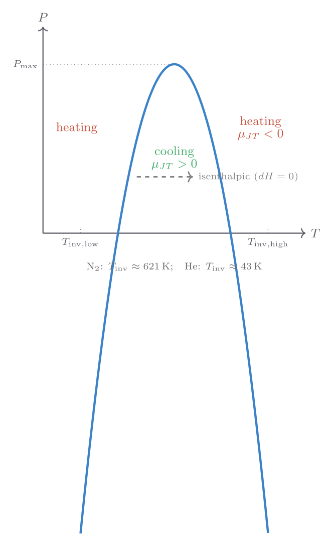
Chapter 17: Free Energies and Available Work
Helmholtz free energy
When a system at constant temperature and volume undergoes a process, the second law requires the entropy of the universe to increase. This can be rephrased as a condition on the system alone. The Helmholtz free energy is defined as
\[ F \equiv U - TS. \]For a system at constant \(T\) and \(V\), spontaneous processes decrease \(F\) (\(dF \leq 0\)), and equilibrium is the state of minimum \(F\). The maximum work extractable from an isothermal, constant-volume process is \(-\Delta F\):
\[ W_\text{max} = -\Delta F \qquad (T, V \text{ fixed}). \]The name “free energy” refers to the portion of internal energy that is “free” to do work, as opposed to the bound energy \(TS\) that is locked up in thermal fluctuations and unavailable.
Gibbs free energy
For processes at constant temperature and pressure — the standard conditions of chemistry — the natural potential is the Gibbs free energy:
\[ G \equiv U + PV - TS = H - TS. \]Spontaneous processes at constant \(T\) and \(P\) decrease \(G\). The maximum non-\(PV\) work extractable is \(-\Delta G\). In a battery, for example, the electrical work delivered equals \(-\Delta G\) of the electrochemical reaction (less than \(-\Delta H\) by the amount \(T\Delta S\)).
The Gibbs free energy determines chemical equilibrium. At equilibrium, \(G\) is minimised and the chemical potential \(\mu_i = (\partial G/\partial N_i)_{T,P,N_{j\neq i}}\) of each species is equalised across all phases. Phase transitions occur when the Gibbs free energies of two phases are equal: ice and water are in equilibrium at the temperature and pressure where \(G_\text{ice}(T,P) = G_\text{liq}(T,P)\).
The maximum work theorem and the Helmholtz free energy
The name “free energy” for \(F\) has a precise meaning. For a process at constant temperature and volume, the first law combined with the second law gives \(\Delta U = Q + W\) and \(Q \leq T\Delta S\), so \(W \geq \Delta U - T\Delta S = \Delta F\). Work done on the system is at least \(\Delta F\), and the maximum work extracted from the system (work done by the system) is at most \(-\Delta F\). Equality holds for a reversible process. The difference \(T\Delta S\) between \(-\Delta F\) and \(-\Delta U\) is the “wasted” entropy cost: even in a perfect isothermal process, the thermal reservoir must absorb entropy from the system, which limits extractable work. This is why some fraction of the internal energy is “bound” and unavailable — the \(TS\) term.
Derivation of \(dG = -S\,dT + V\,dP\)
Starting from \(G = H - TS = U + PV - TS\) and differentiating:
\[ dG = dU + P\,dV + V\,dP - T\,dS - S\,dT. \]Substituting the fundamental relation \(dU = T\,dS - P\,dV\) (valid for quasi-static processes at fixed \(N\)):
\[ dG = T\,dS - P\,dV + P\,dV + V\,dP - T\,dS - S\,dT = V\,dP - S\,dT. \]Therefore \(dG = -S\,dT + V\,dP\), and the natural variables of \(G\) are \(T\) and \(P\). The partial derivatives give \(S = -(\partial G/\partial T)_P\) and \(V = (\partial G/\partial P)_T\). Since \(S \geq 0\), \(G\) decreases as temperature rises at constant pressure. Since \(V > 0\) (for normal matter), \(G\) increases as pressure rises at constant temperature.
Chemical potential and equilibrium
For a system with variable particle number \(N\), the fundamental relation generalises to \(dU = T\,dS - P\,dV + \mu\,dN\), where the chemical potential \(\mu \equiv (\partial U/\partial N)_{S,V}\) is the energy required to add one particle while keeping entropy and volume fixed. In terms of the Gibbs free energy:
\[ \mu = \left(\frac{\partial G}{\partial N}\right)_{T,P}. \]For a pure substance, \(G\) is extensive: \(G(T, P, N) = N\mu(T, P)\), so \(\mu = G/N\) is the Gibbs free energy per particle (or per mole, if \(N\) is measured in moles). This identification makes the Gibbs free energy the correct thermodynamic potential for chemical equilibrium: when a chemical reaction proceeds at constant \(T\) and \(P\), it does so in the direction of decreasing \(G\) (equivalently, decreasing \(\mu_\text{products} - \mu_\text{reactants}\)). Equilibrium is reached when \(\Delta_r G = \sum_i \nu_i\mu_i = 0\), where \(\nu_i\) are the stoichiometric coefficients (positive for products, negative for reactants). The dependence of \(\mu\) on concentration or partial pressure through the ideal-mixing formula \(\mu = \mu^\circ + k_{\mathrm{B}}T\ln(P_i/P^\circ)\) leads directly to the law of mass action and the equilibrium constant.
Chapter 18: Thermodynamic Identities and Maxwell Relations
The fundamental relation and natural variables
The four thermodynamic potentials \(U\), \(H\), \(F\), \(G\) are related by Legendre transforms. Each has natural variables — the variables in which its differential has the simplest form:
\[ dU = T\,dS - P\,dV, \quad dH = T\,dS + V\,dP, \quad dF = -S\,dT - P\,dV, \quad dG = -S\,dT + V\,dP. \]From these, by equality of mixed partial derivatives (\(\partial^2 f/\partial x\,\partial y = \partial^2 f/\partial y\,\partial x\)), one derives the four Maxwell relations:
\[ \left(\frac{\partial T}{\partial V}\right)_S = -\left(\frac{\partial P}{\partial S}\right)_V, \quad \left(\frac{\partial T}{\partial P}\right)_S = \left(\frac{\partial V}{\partial S}\right)_P, \]\[ \left(\frac{\partial S}{\partial V}\right)_T = \left(\frac{\partial P}{\partial T}\right)_V, \quad \left(\frac{\partial S}{\partial P}\right)_T = -\left(\frac{\partial V}{\partial T}\right)_P. \]The last two Maxwell relations are especially practical: they replace difficult direct measurements of entropy derivatives with measurable \(P\)–\(V\)–\(T\) derivatives. For example, how does entropy change with volume at constant temperature? The Maxwell relation says \((\partial S/\partial V)_T = (\partial P/\partial T)_V\) — something that can be calculated from any equation of state.
Explicit derivation of all four Maxwell relations
Each Maxwell relation comes from requiring that a mixed second partial derivative of a thermodynamic potential is symmetric. Starting from \(dU = T\,dS - P\,dV\), the coefficients are \(T = (\partial U/\partial S)_V\) and \(-P = (\partial U/\partial V)_S\). Requiring \(\partial^2 U/\partial V\,\partial S = \partial^2 U/\partial S\,\partial V\):
\[ \left(\frac{\partial T}{\partial V}\right)_S = -\left(\frac{\partial P}{\partial S}\right)_V. \quad (1) \]From \(dH = T\,dS + V\,dP\): coefficients \(T = (\partial H/\partial S)_P\) and \(V = (\partial H/\partial P)_S\). Cross-differentiation:
\[ \left(\frac{\partial T}{\partial P}\right)_S = \left(\frac{\partial V}{\partial S}\right)_P. \quad (2) \]From \(dF = -S\,dT - P\,dV\): coefficients \(-S = (\partial F/\partial T)_V\) and \(-P = (\partial F/\partial V)_T\). Cross-differentiation:
\[ \left(\frac{\partial S}{\partial V}\right)_T = \left(\frac{\partial P}{\partial T}\right)_V. \quad (3) \]From \(dG = -S\,dT + V\,dP\): coefficients \(-S = (\partial G/\partial T)_P\) and \(V = (\partial G/\partial P)_T\). Cross-differentiation:
\[ \left(\frac{\partial S}{\partial P}\right)_T = -\left(\frac{\partial V}{\partial T}\right)_P. \quad (4) \]Worked applications of Maxwell relations
Application 1: entropy change of a van der Waals gas. Using Maxwell relation (3), \((\partial S/\partial V)_T = (\partial P/\partial T)_V\). For the van der Waals equation \(P = Nk_{\mathrm{B}}T/(V - Nb) - aN^2/V^2\), the derivative is \((\partial P/\partial T)_V = Nk_{\mathrm{B}}/(V - Nb)\). Therefore the isothermal entropy change from \(V_1\) to \(V_2\) is
\[ \Delta S = \int_{V_1}^{V_2}\!\left(\frac{\partial P}{\partial T}\right)_V dV = Nk_{\mathrm{B}}\ln\frac{V_2 - Nb}{V_1 - Nb}. \]Note the appearance of the excluded volume \(Nb\) rather than \(V\) itself — the molecules cannot access the excluded volume, so only the free volume contributes to entropy.
Application 2: deriving \(C_P - C_V\) via Maxwell relations. The general identity \(C_P - C_V = [(\partial U/\partial V)_T + P](\partial V/\partial T)_P\) was encountered in Chapter 3. Using the Maxwell relation \((\partial S/\partial V)_T = (\partial P/\partial T)_V\) and the thermodynamic identity \((\partial U/\partial V)_T = T(\partial P/\partial T)_V - P\) (derived by substituting \(dS = \delta Q/T\) into \(dU = T\,dS - P\,dV\)):
\[ C_P - C_V = T\left(\frac{\partial P}{\partial T}\right)_V\!\left(\frac{\partial V}{\partial T}\right)_P. \]Using the triple product rule \((\partial P/\partial T)_V(\partial T/\partial V)_P(\partial V/\partial P)_T = -1\), we can write \((\partial P/\partial T)_V = -(\partial V/\partial T)_P/(\partial V/\partial P)_T = \beta V/(-\kappa_T V) = \beta/\kappa_T V\). Wait — more carefully: \((\partial P/\partial T)_V = \beta/\kappa_T\) via the triple product rule applied to \(P(V, T)\). Then:
\[ C_P - C_V = T \cdot \frac{\beta}{\kappa_T}\cdot \beta V = \frac{TV\beta^2}{\kappa_T}, \]recovering the standard result. This derivation, carried out entirely through Maxwell relations and the triple product rule, illustrates how the four Maxwell relations serve as the main analytical tools of classical thermodynamics.
General relation between heat capacities
Using the Maxwell relation \((\partial S/\partial V)_T = (\partial P/\partial T)_V\) and the triple product rule for \(P\), \(V\), \(T\), one derives the general result
\[ C_P - C_V = \frac{TV\beta^2}{\kappa_T}, \]where \(\beta = (1/V)(\partial V/\partial T)_P\) is the thermal expansivity and \(\kappa_T = -(1/V)(\partial V/\partial P)_T\) is the isothermal compressibility. This general formula reduces to the Mayer relation \(C_P - C_V = Nk_{\mathrm{B}}\) for an ideal gas, and provides a way to deduce \(C_V\) from measured \(C_P\), \(\beta\), and \(\kappa_T\) for any material — useful because \(C_V\) is hard to measure directly for solids and liquids.
Chapter 19: Clausius-Clapeyron and Phase Boundaries
Conditions for phase equilibrium
Two phases \(\alpha\) and \(\beta\) of a substance coexist in equilibrium when their temperatures, pressures, and chemical potentials are equal: \(T_\alpha = T_\beta\), \(P_\alpha = P_\beta\), \(\mu_\alpha(T,P) = \mu_\beta(T,P)\). The last condition defines a curve in the \(P\)–\(T\) plane — the phase boundary.
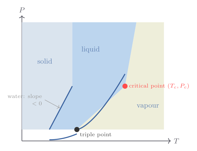
The three phases meet at the triple point — for water, at 273.16 K and 611.7 Pa. Above the critical point (374 °C, 218 atm for water), the distinction between liquid and gas vanishes. The slope of the phase boundary is given by the Clausius-Clapeyron equation:
\[ \frac{dP}{dT} = \frac{L}{T\Delta V} = \frac{\Delta S}{\Delta V}, \]where \(L = T\Delta S\) is the molar latent heat and \(\Delta V\) is the molar volume difference between phases. This equation can be derived directly from \(\mu_\alpha = \mu_\beta\) and \(d\mu = -S\,dT + V\,dP\).
Implications of the Clausius-Clapeyron equation
For the liquid-vapour transition, \(\Delta V \approx V_\text{gas} \approx RT/P\) (treating the vapour as ideal), giving
\[ \frac{d\ln P}{dT} = \frac{L}{RT^2}, \]which integrates to the Antoine equation \(\ln P \approx -L/RT + \text{const}\). Vapour pressure increases exponentially with temperature — boiling occurs when the vapour pressure equals the external pressure, which is why water boils at 70 °C at high altitude (where atmospheric pressure is lower) and at 120 °C in a pressure cooker.
The sign of \(dP/dT\) is determined by \(\Delta V\). For most substances \(V_\text{liquid} < V_\text{solid}\), so \(\Delta V > 0\) and the melting curve has a positive slope. Water is famous for having \(V_\text{liquid} > V_\text{solid}\) (ice is less dense than water), giving a negative slope: increasing pressure lowers the melting point. This is occasionally cited as explaining ice skating (pressure from the blade melts ice) — but the pressure required to lower the melting point by even 1 °C is about 130 atm, far more than a skater exerts. The real lubricant is a thin quasi-liquid layer that forms on ice surfaces even without applied pressure.
Full derivation of the Clausius-Clapeyron equation
Along the coexistence curve, the chemical potentials of the two phases are equal: \(\mu_\alpha(T, P) = \mu_\beta(T, P)\). Moving to a nearby point on the curve at \((T + dT, P + dP)\), the equality must still hold:
\[ \mu_\alpha(T + dT, P + dP) = \mu_\beta(T + dT, P + dP). \]Expanding each side to first order using \(d\mu = -S_m\,dT + V_m\,dP\) (from \(dG = -S\,dT + V\,dP\) per mole, with \(\mu = G/N\)):
\[ \mu_\alpha - S_{m,\alpha}\,dT + V_{m,\alpha}\,dP = \mu_\beta - S_{m,\beta}\,dT + V_{m,\beta}\,dP. \]Since \(\mu_\alpha = \mu_\beta\) on the curve, those terms cancel. Rearranging:
\[ (V_{m,\alpha} - V_{m,\beta})\,dP = (S_{m,\alpha} - S_{m,\beta})\,dT, \]\[ \frac{dP}{dT} = \frac{\Delta S_m}{\Delta V_m} = \frac{L}{T\,\Delta V_m}, \]where \(L = T\Delta S_m\) is the molar latent heat and \(\Delta V_m = V_{m,\alpha} - V_{m,\beta}\) is the molar volume difference.
Numerical applications for water
For the liquid-vapour boundary: treating the vapour as ideal, \(V_{m,\text{gas}} \approx RT/P \gg V_{m,\text{liq}}\), so \(\Delta V_m \approx RT/P\). The Clausius-Clapeyron equation becomes
\[ \frac{d\ln P}{dT} = \frac{L_\text{vap}}{RT^2}. \]With \(L_\text{vap} = 40\,700\ \text{J mol}^{-1}\) and \(R = 8.314\ \text{J mol}^{-1}\text{K}^{-1}\), at \(T = 373\ \text{K}\):
\[ \frac{d\ln P}{dT} = \frac{40\,700}{8.314 \times 373^2} \approx 3.52 \times 10^{-2}\ \text{K}^{-1}. \]A 1 K rise in temperature increases \(\ln P\) by 0.035, so the vapour pressure increases by about 3.5% per kelvin near the boiling point. This explains why boiling occurs at a lower temperature at high altitude: at 3500 m, atmospheric pressure is about 650 mbar instead of 1013 mbar, and the boiling point of water drops to approximately 90 °C.
For the solid-liquid boundary: \(\Delta V_m = V_{m,\text{liq}} - V_{m,\text{solid}} = (1/1000 - 1/917)\ \text{m}^3\text{mol}^{-1} \times 0.018\ \text{kg mol}^{-1} \approx -1.63 \times 10^{-6}\ \text{m}^3\text{mol}^{-1}\). With \(L_\text{fus} = 6010\ \text{J mol}^{-1}\) and \(T = 273\ \text{K}\):
\[ \frac{dP}{dT} = \frac{6010}{273 \times (-1.63 \times 10^{-6})} \approx -1.35 \times 10^7\ \text{Pa K}^{-1} = -134\ \text{atm K}^{-1}. \]The melting point of ice shifts by only \(-0.0075\ \text{K atm}^{-1}\) — a tiny effect. A skater exerting 100 atm would lower the melting point by only 0.75 °C, insufficient in a rink held at \(-15\) °C. Clearly, pressure-induced melting is not the dominant mechanism of lubrication in ice skating.
Part IV: Real Substances and Critical Phenomena
Chapter 20: Real Gases — Virial Expansion and the van der Waals Equation
Beyond the ideal gas
The ideal gas law ignores two physical facts: molecules have finite size, and they attract one another at short range. At low densities these corrections are negligible; at high densities they become important. The virial expansion is the systematic way to include them:
\[ \frac{PV}{Nk_{\mathrm{B}}T} = 1 + \frac{B_2(T)}{(V/N)} + \frac{B_3(T)}{(V/N)^2} + \cdots, \]where \(B_2(T)\), \(B_3(T)\), … are the virial coefficients, which depend on temperature and encode progressively more complex molecular interactions. \(B_2\) comes from pairwise interactions and is the most important correction at moderate densities. At high temperatures, repulsive cores dominate and \(B_2 > 0\) (gas is harder to compress than ideal); at low temperatures, attractive interactions dominate and \(B_2 < 0\) (easier to compress). The temperature at which \(B_2 = 0\) — the Boyle temperature — is where the first correction vanishes and the ideal gas law happens to work well over a wide range of pressures.
The van der Waals equation
The van der Waals equation (1873) is a simple mean-field correction to the ideal gas law:
\[ \left(P + \frac{aN^2}{V^2}\right)\!\left(V - Nb\right) = Nk_{\mathrm{B}}T. \]The parameter \(b\) is the excluded volume per molecule (each molecule excludes a volume \(b\) from others), accounting for finite molecular size. The parameter \(a\) accounts for long-range attractions: molecules in the bulk are pulled symmetrically in all directions, but those near the wall experience a net inward pull, reducing the pressure by an amount proportional to the square of the density, \(a(N/V)^2\).
At high temperatures and low densities, the van der Waals equation reduces to the ideal gas law. At low temperatures and high densities it predicts — crucially — that \((\partial P/\partial V)_T\) can become positive: the pressure increases when the volume increases at constant temperature. This unphysical behaviour (a mechanically unstable state) signals the onset of phase separation: the system splits into liquid and gas rather than occupying those unstable states.
Physical interpretation of the second virial coefficient \(B_2(T)\)
The second virial coefficient can be computed from the pair interaction potential \(u(r)\) between two molecules via the cluster-integral formula:
\[ B_2(T) = -2\pi\!\int_0^\infty\!\left(e^{-u(r)/k_{\mathrm{B}}T} - 1\right)\!r^2\,dr. \]For a pair potential that is strongly repulsive at short range and weakly attractive at long range (like the Lennard-Jones potential), the integrand is \(-1\) for \(r < r_\text{min}\) (where the core repulsion keeps molecules apart) and slightly positive for \(r > r_\text{min}\) (the attractive tail). At high temperatures, \(k_{\mathrm{B}}T \gg |u_\text{min}|\) and the attractive part of the integrand is negligible: \(e^{-u/k_{\mathrm{B}}T} - 1 \approx 0\) in the attractive region. The integral is dominated by the hard-core excluded volume, giving \(B_2 \approx 2\pi r_\text{core}^3/3 = b/2 > 0\) (using van der Waals notation, \(b = 4 \times (4\pi r_\text{core}^3/3)/1\) for one mole). At low temperatures, the attractive tail contributes negatively, reducing \(B_2\) and eventually making it negative. The Boyle temperature \(T_B\) at which \(B_2 = 0\) satisfies roughly \(k_{\mathrm{B}}T_B \sim |u_\text{min}|\); for nitrogen, \(T_B \approx 330\ \text{K}\).
Deriving the van der Waals pressure from pair interactions
The van der Waals parameter \(a\) can be related to the pair potential. In a liquid of density \(n = N/V\), a molecule near the wall experiences a net inward force due to intermolecular attractions from the bulk. The pressure reduction (the internal pressure) at the wall is proportional to the number of molecules per unit volume times the range-integrated attraction:
\[ P_\text{internal} = \frac{a n^2}{1} = a\left(\frac{N}{V}\right)^2, \]giving \(P_\text{real} = P_\text{ideal} - a(N/V)^2\). The relation between \(a\) and the pair potential is \(a = -2\pi\!\int_{r_\text{core}}^\infty u(r)\,r^2\,dr\), where the integral picks up the attractive tail of \(u(r)\) (which is negative, making \(a > 0\)).
The excluded volume parameter \(b\) arises because two molecules cannot overlap. If each molecule is modelled as a hard sphere of radius \(r_\text{hs}\), then two molecules cannot be closer than \(2r_\text{hs}\). The volume excluded to the centre of one molecule by the presence of another is \((4/3)\pi(2r_\text{hs})^3 = 8 V_\text{mol}\), where \(V_\text{mol}\) is the volume of a single molecule. Since this exclusion is shared between two molecules, the excluded volume per molecule is \(4V_\text{mol}\), and for \(N\) molecules: \(b = 4N_\text{A}V_\text{mol}\) per mole. The van der Waals equation then arises as the leading-order correction to the ideal gas law that simultaneously accounts for finite molecular volume and long-range attractions.
The virial expansion and its domain of validity
The virial expansion \(PV/Nk_{\mathrm{B}}T = 1 + B_2(T)/(V/N) + B_3(T)/(V/N)^2 + \ldots\) is a power series in density. For gases at ordinary pressures, the first correction is sufficient. For example, at \(T = 300\ \text{K}\) and \(P = 10\ \text{atm}\), nitrogen has \(n = P/(k_{\mathrm{B}}T) \approx 2.4 \times 10^{26}\ \text{m}^{-3}\) and \(B_2(300\ \text{K}) \approx -4 \times 10^{-6}\ \text{m}^3\text{mol}^{-1}/N_A \approx -6.6 \times 10^{-30}\ \text{m}^3\). The correction \(nB_2 \approx -1.6 \times 10^{-3}\) — a 0.16% deviation from ideality, well within measurement precision for most purposes. At 100 atm, the correction grows to roughly 1.6%, and higher virial coefficients become necessary. The series diverges at the critical density, where liquid-gas phase separation occurs, so the virial expansion is restricted to the single-phase fluid region.
Chapter 21: Maxwell Construction, Critical Point, and the Law of Corresponding States
Maxwell construction and phase coexistence
The van der Waals isotherm at low temperatures has an S-shaped region with a local maximum and minimum. Real isotherms have a flat plateau in this region — the liquid-vapour coexistence pressure at which both phases have the same chemical potential. The Maxwell equal-area construction determines this pressure: one draws a horizontal line on the \(P\)–\(V\) isotherm such that the area of the loop above the line equals the area below it. This equal-area condition follows from the requirement that the Gibbs free energy of the two phases be equal.
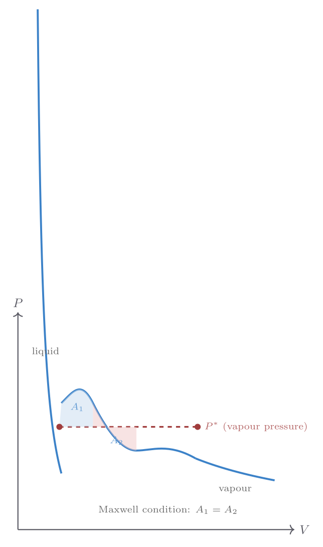
The critical point
As the temperature increases, the liquid and vapour densities converge. At the critical temperature \(T_c\), the two coexisting densities become equal and the phase transition disappears — there is a single fluid phase. The critical point corresponds to an inflection point in the van der Waals isotherm:
\[ \left(\frac{\partial P}{\partial V}\right)_{T_c} = 0, \qquad \left(\frac{\partial^2 P}{\partial V^2}\right)_{T_c} = 0. \]Solving these conditions for the van der Waals equation gives
\[ T_c = \frac{8a}{27k_{\mathrm{B}}b}, \qquad P_c = \frac{a}{27b^2}, \qquad V_c = 3Nb. \]Near the critical point, the compressibility diverges, density fluctuations grow large, and the fluid strongly scatters light — the phenomenon of critical opalescence seen near the critical point of many binary mixtures.
Law of corresponding states
Expressing the van der Waals equation in terms of reduced variables \(T_r = T/T_c\), \(P_r = P/P_c\), \(V_r = V/V_c\) yields an equation with no material-specific parameters:
\[ \left(P_r + \frac{3}{V_r^2}\right)(3V_r - 1) = 8T_r. \]This is the law of corresponding states: all van der Waals gases obey the same reduced equation of state. Different gases at the same \(T_r\) and \(P_r\) have the same \(V_r\). The law is approximately obeyed by many real gases — a striking success of mean-field theory. It fails near the critical point, where fluctuations dominate and mean-field theory breaks down.
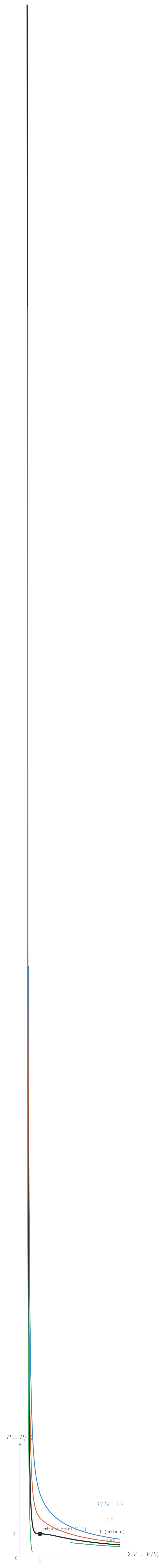
Chapter 22: Critical Exponents, Scaling, and Landau Mean-Field Theory
Critical exponents
Near the critical point, thermodynamic quantities exhibit power-law behaviour characterised by critical exponents. The order parameter for the liquid-vapour transition is the density difference \(\rho_\text{liq} - \rho_\text{gas}\):
\[ \rho_\text{liq} - \rho_\text{gas} \sim (T_c - T)^\beta, \quad \kappa_T \sim |T - T_c|^{-\gamma}, \quad C_V \sim |T - T_c|^{-\alpha}. \]Mean-field theory (van der Waals or Landau) predicts \(\beta = 1/2\), \(\gamma = 1\), \(\alpha = 0\) (discontinuous jump). Experiment gives \(\beta \approx 0.326\), \(\gamma \approx 1.24\), \(\alpha \approx 0.11\) for the 3D liquid-gas universality class — clearly different from mean-field values. The critical exponents are universal: they are the same for all transitions in the same universality class, regardless of the specific material or microscopic interactions. This universality was one of the great theoretical triumphs of the 1970s (Wilson’s renormalisation group).
Landau theory
Landau’s theory of phase transitions (1937) provides a general framework: expand the Gibbs free energy as a power series in an order parameter \(\phi\) (which measures the degree of symmetry-breaking):
\[ G = G_0 + a_2(T)\phi^2 + a_4\phi^4 + \cdots \]For a second-order (continuous) transition, \(a_4 > 0\) and \(a_2\) changes sign at \(T_c\): \(a_2 \propto (T - T_c)\). Above \(T_c\), the minimum is at \(\phi = 0\) (disordered phase); below \(T_c\), symmetry is spontaneously broken and \(\phi \neq 0\). This framework predicts mean-field exponents and is exact in sufficiently high spatial dimensions (\(d > 4\) for the Ising universality class). Below the upper critical dimension, fluctuations modify the exponents, and renormalisation-group methods are needed.
For first-order transitions (e.g., the liquid-vapour transition below \(T_c\)), a term \(a_3\phi^3\) appears and the transition involves a discontinuous jump in the order parameter, latent heat, and a two-phase coexistence region — all features captured qualitatively by the van der Waals equation.
Critical exponents in detail
Each critical exponent describes the leading power-law singularity of a thermodynamic observable as the critical point is approached. The four primary exponents are:
Exponent \(\beta\): The order parameter \(\Delta\rho \equiv \rho_\text{liq} - \rho_\text{gas}\) vanishes as \(\Delta\rho \sim (T_c - T)^\beta\) for \(T \to T_c^-\). Mean-field (van der Waals) theory predicts \(\beta = 1/2\) from the cubic form of the van der Waals isotherm near the critical point. The exact 3D Ising value is \(\beta \approx 0.326\). This difference is not small — the square root versus the 1/3 power give qualitatively different rates of vanishing.
Exponent \(\gamma\): The isothermal compressibility \(\kappa_T\) diverges on both sides of \(T_c\): \(\kappa_T \sim |T - T_c|^{-\gamma}\). Mean-field theory gives \(\gamma = 1\); the 3D Ising value is \(\gamma \approx 1.237\). The divergence of \(\kappa_T\) is associated with the divergence of density fluctuations: near the critical point, droplets of liquid and bubbles of gas appear on all length scales, and the fluid becomes opaque (critical opalescence).
Exponent \(\alpha\): The specific heat at constant volume diverges (or shows a cusp) as \(C_V \sim |T - T_c|^{-\alpha}\). Mean-field theory predicts \(\alpha = 0\) (a finite discontinuity, not a divergence). The 3D Ising value \(\alpha \approx 0.110\) corresponds to a weak divergence, much harder to observe experimentally.
Exponent \(\delta\): Along the critical isotherm \(T = T_c\), the pressure deviates from the critical pressure as \(P - P_c \sim |\rho - \rho_c|^\delta\). Mean-field gives \(\delta = 3\); the 3D value is \(\delta \approx 4.79\).
The scaling hypothesis
The scaling hypothesis asserts that near the critical point, the singular part of the free energy has a homogeneous (scaling) form. This leads to relations between the exponents — the scaling laws. For example:
\[ \alpha + 2\beta + \gamma = 2 \quad (\text{Rushbrooke's equality}), \qquad \delta = 1 + \gamma/\beta \quad (\text{Widom's equality}). \]These are not independent predictions — they follow from assuming that the free energy is a generalised homogeneous function of \((T - T_c)\) and an ordering field. The scaling hypothesis was empirically confirmed before its theoretical basis (the renormalisation group) was established. With mean-field values \(\alpha = 0\), \(\beta = 1/2\), \(\gamma = 1\): Rushbrooke gives \(0 + 1 + 1 = 2\) ✓; Widom gives \(\delta = 1 + 1/(1/2) = 3\) ✓. With 3D Ising values: \(0.110 + 2(0.326) + 1.237 \approx 1.999 \approx 2\) — a remarkable agreement with theory.
Universality classes
The concept of universality — that the critical exponents are the same for all materials in the same class, regardless of their microscopic differences — is one of the deepest insights of statistical mechanics. A universality class is determined by only a few features: the spatial dimension \(d\) of the system, the symmetry of the order parameter (its dimension \(n\)), and whether interactions are short- or long-range.
The 3D Ising class (order parameter: scalar, \(n = 1\)) includes the liquid-gas transition, uniaxial ferromagnets, binary alloys, and polymer solutions near their critical points. All have \(\beta \approx 0.326\), \(\gamma \approx 1.237\), regardless of whether they involve water, iron, or polymer chains. The 3D Heisenberg class (\(n = 3\), vector order parameter) describes isotropic ferromagnets. The 2D Ising class (exactly solvable by Onsager’s method) has \(\beta = 1/8\), \(\gamma = 7/4\) — very different from 3D. Mean-field theory is exact for \(d \geq 4\) (above the upper critical dimension), where fluctuations are irrelevant to the critical behaviour.
Part V: Quantum Statistics
Chapter 23: Quantum Ideal Gases — Bose-Einstein and Fermi-Dirac Distributions
Why classical statistics fails at low temperature
The Boltzmann distribution treats gas molecules as distinguishable and ignores quantum interference between their wavefunctions. This works when the typical separation between particles, \((V/N)^{1/3}\), is much larger than the thermal de Broglie wavelength \(\lambda_\text{th} = h/\sqrt{2\pi mk_{\mathrm{B}}T}\). The failure condition \(\lambda_\text{th} \gtrsim (V/N)^{1/3}\) — quantum degeneracy — is reached at low temperatures or high densities.
Two fundamentally different types of quantum statistics arise depending on the spin of the particles. Bosons (integer spin: photons, \(^4\)He atoms, Cooper pairs) are described by symmetric wavefunctions and can occupy the same state in arbitrary numbers. Fermions (half-integer spin: electrons, protons, \(^3\)He atoms) are described by antisymmetric wavefunctions and obey the Pauli exclusion principle: no two fermions can occupy the same state.
Derivation of the distributions
For a grand-canonical ensemble (fixed \(T\), \(V\), chemical potential \(\mu\)), the mean occupation number of a single-particle state with energy \(\epsilon\) is
\[ \bar{n}(\epsilon) = \frac{1}{e^{(\epsilon - \mu)/k_{\mathrm{B}}T} \pm 1}, \]with \(+\) for Fermi-Dirac (fermions) and \(-\) for Bose-Einstein (bosons). The chemical potential \(\mu\) adjusts to give the correct total number of particles.
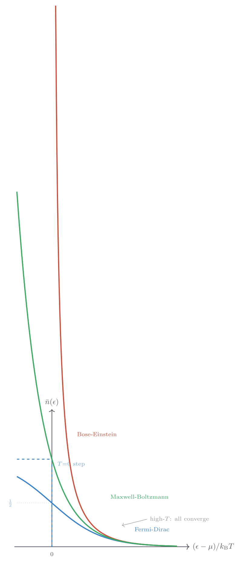
At high temperatures and low densities, both quantum distributions reduce to the Maxwell-Boltzmann result \(\bar{n} \approx e^{-(\epsilon-\mu)/k_{\mathrm{B}}T}\) — the classical limit.
Fermi-Dirac gas: electrons in metals
For electrons in a metal at \(T = 0\), all states up to the Fermi energy \(\epsilon_F\) are filled and all states above are empty — a step function. The Fermi energy for a free electron gas is
\[ \epsilon_F = \frac{\hbar^2}{2m}\left(3\pi^2 n\right)^{2/3}, \]where \(n\) is the electron density. For copper, \(\epsilon_F \approx 7\ \text{eV}\), corresponding to a Fermi temperature \(T_F = \epsilon_F/k_{\mathrm{B}} \approx 80\,000\ \text{K}\). Room temperature is far below \(T_F\), so the electron gas is highly degenerate. The heat capacity of the electron gas is linear in \(T\) at low temperature, \(C_V = \gamma T\), contributing a measurable but small linear term to the total specific heat at low \(T\) (the lattice contribution goes as \(T^3\)).
Bose-Einstein condensation
For bosons, the chemical potential must satisfy \(\mu \leq \epsilon_\text{min}\) to keep all occupation numbers non-negative. As temperature decreases at fixed density, \(\mu\) rises. At the condensation temperature \(T_c\), \(\mu\) reaches the ground-state energy, and a macroscopic fraction of the particles condenses into the ground state — Bose-Einstein condensation (BEC). For an ideal gas,
\[ T_c = \frac{2\pi\hbar^2}{mk_{\mathrm{B}}}\left(\frac{n}{2.612}\right)^{2/3}. \]BEC was observed in ultracold atomic vapours in 1995 (Anderson, Ensher, Matthews, Wieman, Cornell), winning the 2001 Nobel Prize. Superfluid \(^4\)He (below 2.17 K) is a strongly interacting BEC. Superconductivity is Cooper-pair BEC.
The contrast between Fermi-Dirac and Bose-Einstein statistics has profound physical consequences. For a free Fermi gas at \(T = 0\), the pressure does not vanish — this degeneracy pressure comes entirely from the Pauli exclusion principle forcing fermions into states of successively higher kinetic energy. White dwarf stars are supported against gravitational collapse by electron degeneracy pressure; when the white dwarf mass exceeds the Chandrasekhar limit (\(\approx 1.4\ M_\odot\)), even degeneracy pressure is insufficient and the star collapses further, potentially producing a neutron star supported by neutron degeneracy pressure. For a Bose gas, by contrast, there is no such pressure at \(T = 0\) in the non-interacting limit — all particles condense into the single lowest-energy state. The profound difference between a universe of fermions (which resist compression and form stable atoms, molecules, and stars) and one of bosons (which would all condense into a single quantum state) is perhaps the most consequential consequence of quantum statistics for the large-scale structure of matter.
Chapter 24: The Photon Gas and the Debye Model of Solids
Photons as massless bosons
Photons are bosons with zero chemical potential (\(\mu = 0\)) because the number of photons in a cavity is not fixed — photons can be absorbed and re-emitted. The Bose-Einstein distribution with \(\mu = 0\) gives the mean number of photons in a mode with frequency \(\nu\):
\[ \bar{n}(\nu) = \frac{1}{e^{h\nu/k_{\mathrm{B}}T} - 1}. \]The energy per mode is \(h\nu\,\bar{n}(\nu)\). Multiplying by the density of modes in a cavity and integrating gives the Planck spectrum — the spectral energy density of blackbody radiation — which is derived properly in Chapter 26.
The Debye model
Einstein’s model of a solid assumed all oscillators have the same frequency \(\omega_E\). A better model, due to Debye (1912), allows a continuous distribution of frequencies up to a maximum Debye frequency \(\omega_D\), which corresponds to the shortest possible wavelength (one oscillation per lattice spacing). The density of modes is \(g(\omega) \propto \omega^2\) for \(\omega \leq \omega_D\), giving
\[ C_V = 9Nk_{\mathrm{B}}\left(\frac{T}{T_D}\right)^3\!\int_0^{T_D/T}\!\!\!\frac{x^4 e^x}{(e^x - 1)^2}\,dx, \quad x = \frac{\hbar\omega}{k_{\mathrm{B}}T}, \]where \(T_D = \hbar\omega_D/k_{\mathrm{B}}\) is the Debye temperature. At high \(T\), this reduces to the Dulong-Petit value \(3Nk_{\mathrm{B}}\); at low \(T\), \(C_V \propto T^3\) — the celebrated Debye \(T^3\) law, experimentally confirmed for almost all crystalline solids below about \(T_D/50\). Typical Debye temperatures range from 90 K (lead) to 2230 K (diamond).
Part VI: Thermal Radiation and the Temperature of the Earth
Chapter 25: Thermodynamics of Thermal Radiation
Radiation as a thermodynamic system
Any body at finite temperature emits electromagnetic radiation simply by virtue of the thermal motion of its charged constituents — this is thermal radiation. The radiation field inside a cavity in equilibrium with its walls at temperature \(T\) constitutes a well-defined thermodynamic system: the photon gas. Its properties can be derived entirely from thermodynamic arguments before specifying the spectral distribution.
The energy density \(u\) of isotropic radiation in a cavity satisfies a powerful constraint from thermodynamics. Because photons are massless and travel at speed \(c\), the radiation pressure is \(P_\text{rad} = u/3\). Using the thermodynamic identity \((\partial U/\partial V)_T = T(\partial P/\partial T)_V - P\) (derived from the Maxwell relation on \(F\)), and substituting \(U = uV\) and \(P = u/3\):
\[ u = T\frac{du/3}{dT} - \frac{u}{3}, \qquad \Rightarrow\qquad \frac{du}{u} = 4\frac{dT}{T}, \qquad \Rightarrow\qquad u \propto T^4. \]This is the Stefan-Boltzmann law in disguise: the total energy density of blackbody radiation is proportional to \(T^4\), derived purely from thermodynamics without any knowledge of the spectral distribution. The emitted power per unit area (the emissive power or irradiance) of a blackbody surface is
\[ j = \sigma T^4, \qquad \sigma = \frac{2\pi^5 k_{\mathrm{B}}^4}{15 c^2 h^3} \approx 5.67 \times 10^{-8}\ \text{W m}^{-2}\text{K}^{-4}, \]where \(\sigma\) is the Stefan-Boltzmann constant.
Chapter 26: The Planck Spectrum and Wien’s Law
Wien’s displacement law
The spectral distribution of blackbody radiation — how the energy is distributed across frequencies — is constrained by a scaling argument. The energy density per unit frequency, \(u_\nu(\nu, T)\), must have the form
\[ u_\nu(\nu, T) = \nu^3 f(\nu/T) \]for some universal function \(f\) — this is Wien’s displacement law in its general form, derivable from the combination of the Stefan-Boltzmann \(T^4\) law and the radiation pressure relation. The specific spectral peak shifts with temperature: the frequency (or wavelength) at maximum emission satisfies
\[ \lambda_\text{max} T = b, \qquad b \approx 2.898 \times 10^{-3}\ \text{m}\,\text{K}. \]Wien’s displacement law explains why: the Sun (\(T \approx 5778\ \text{K}\)) peaks at visible wavelengths (\(\lambda_\text{max} \approx 500\ \text{nm}\)); a tungsten filament at 3000 K peaks in the near-infrared, emitting white light only because the high-frequency tail extends into the visible; the Earth at 288 K peaks in the mid-infrared around 10 μm; and the cosmic microwave background at 2.725 K peaks at about 1 mm.
Planck’s distribution
Classical physics predicts that \(u_\nu \propto \nu^2 k_{\mathrm{B}}T\) — the Rayleigh-Jeans law, which diverges as \(\nu \to \infty\) (the ultraviolet catastrophe). This catastrophe indicates a fundamental failure of classical equipartition applied to radiation modes.
Planck’s 1900 hypothesis — that each oscillator of frequency \(\nu\) can absorb or emit energy only in quanta \(h\nu\) — gives the mean energy per mode:
\[ \langle E(\nu, T) \rangle = \frac{h\nu}{e^{h\nu/k_{\mathrm{B}}T} - 1}, \]which reduces to \(k_{\mathrm{B}}T\) at low frequencies (classical limit) and vanishes exponentially at high frequencies (quantum suppression). The full Planck distribution is
\[ u_\nu(\nu, T) = \frac{8\pi h \nu^3}{c^3}\cdot\frac{1}{e^{h\nu/k_{\mathrm{B}}T} - 1}. \]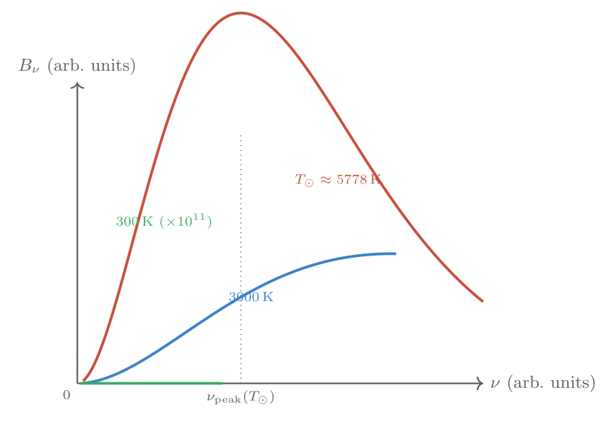
Integrating over all frequencies recovers the Stefan-Boltzmann \(T^4\) law with the numerical constant determined:
\[ u = \frac{8\pi^5 k_{\mathrm{B}}^4}{15 c^3 h^3} T^4. \]Planck’s 1900 paper introducing the quantum hypothesis is conventionally taken as the birth of quantum mechanics. The ultraviolet catastrophe was resolved not by adjusting the radiation theory but by fundamentally quantising the exchange of energy between matter and radiation.
The Planck distribution can be derived from first principles using the Bose-Einstein distribution for photons. Photons are massless bosons with two polarisation states per mode. The density of modes in a cavity of volume \(V\) with frequency between \(\nu\) and \(\nu + d\nu\) is \(g(\nu) = 8\pi V\nu^2/c^3\) (including the factor of 2 for polarisations). Multiplying by the mean energy per photon mode \(h\nu/(e^{h\nu/k_{\mathrm{B}}T} - 1)\) and dividing by \(V\) gives the spectral energy density:
\[ u_\nu(\nu, T) = g(\nu)\frac{h\nu}{e^{h\nu/k_{\mathrm{B}}T}-1}\cdot\frac{1}{V} = \frac{8\pi h\nu^3}{c^3}\cdot\frac{1}{e^{h\nu/k_{\mathrm{B}}T}-1}, \]which is the Planck formula. The factor \(\mu = 0\) for photons reflects the fact that photons can be created and destroyed by the cavity walls — their number is not conserved. This distinguishes photons from, for example, helium atoms in a box, where the number is fixed and \(\mu \neq 0\).
Emissivity and real surfaces
A blackbody is an ideal absorber and emitter. Real surfaces are characterised by their emissivity \(\varepsilon \in [0, 1]\), defined as the ratio of their emitted power to that of a blackbody at the same temperature: \(j = \varepsilon\sigma T^4\). By Kirchhoff’s law, a body in thermal equilibrium must absorb the same fraction of incident radiation as it emits — so emissivity equals absorptivity at each wavelength. This equivalence is a consequence of the second law of thermodynamics: if a body absorbed more than it emitted at some wavelength, it could be used to violate Clausius’s statement by spontaneously directing radiation from a cool to a hot body. A white surface reflects visible light (\(\varepsilon_\text{vis} \approx 0\)) but has high emissivity in the infrared (\(\varepsilon_\text{IR} \approx 0.95\)); a polished metal has low emissivity at all wavelengths, which is why aluminised mylar emergency blankets are effective at retaining body heat.
Chapter 27: Radiative Balance, the Sun, and Earth’s Temperature
Solar luminosity and effective temperature
The Sun radiates as an approximate blackbody with surface temperature \(T_\odot \approx 5778\ \text{K}\). Its total luminosity is
\[ L_\odot = 4\pi R_\odot^2 \sigma T_\odot^4 \approx 3.85 \times 10^{26}\ \text{W}, \]where \(R_\odot \approx 6.96 \times 10^8\ \text{m}\). At Earth’s orbital distance \(d \approx 1.496 \times 10^{11}\ \text{m}\) (1 AU), the solar irradiance (the solar constant) is
\[ S = \frac{L_\odot}{4\pi d^2} \approx 1361\ \text{W m}^{-2}. \]Earth’s equilibrium temperature
Earth intercepts solar power over its cross-sectional area \(\pi R_\oplus^2\) but re-radiates over its full spherical surface area \(4\pi R_\oplus^2\). With albedo \(A\) (fraction of solar radiation reflected) and emissivity \(\varepsilon\), the energy balance gives
\[ \pi R_\oplus^2 S(1 - A) = 4\pi R_\oplus^2 \varepsilon\sigma T_\oplus^4, \]which simplifies to
\[ T_\oplus = \left(\frac{S(1-A)}{4\varepsilon\sigma}\right)^{1/4}. \]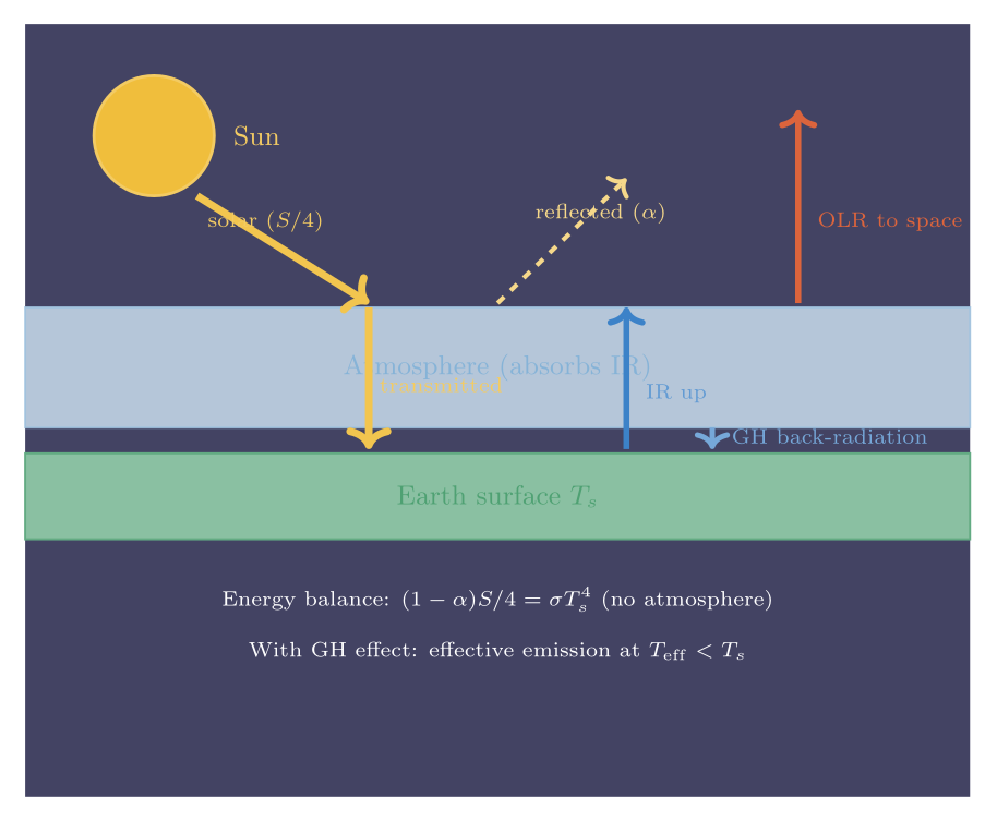
With \(A \approx 0.30\) (Earth’s mean albedo) and \(\varepsilon = 1\):
\[ T_\oplus \approx \left(\frac{1361 \times 0.70}{4 \times 5.67 \times 10^{-8}}\right)^{1/4} \approx 255\ \text{K} = -18\text{ °C}. \]Earth’s actual mean surface temperature is about \(288\ \text{K} = +15\text{ °C}\) — some 33 K warmer than this simple calculation predicts.
The greenhouse effect
The discrepancy arises from the greenhouse effect: the atmosphere is largely transparent to incoming short-wave solar radiation but partially opaque to the long-wave infrared radiation emitted by Earth’s surface. Greenhouse gases — primarily water vapour, carbon dioxide, methane, nitrous oxide, and ozone — absorb and re-emit infrared photons, effectively reducing the emissivity of the atmosphere to infrared and trapping heat near the surface.
A simple two-layer model illustrates this. Suppose the atmosphere absorbs all surface IR radiation and re-emits half upward (to space) and half downward (to the surface). Then the surface must emit \(2\sigma T_\text{surface}^4\) to maintain energy balance (half goes back to it), while the atmosphere emits \(\sigma T_\oplus^4 = S(1-A)/4\) to space. Solving gives \(T_\text{surface} = 2^{1/4} T_\oplus \approx 303\ \text{K}\). This overestimates the warming because the real atmosphere is only partially opaque, but it captures the physics: the greenhouse effect elevates the surface temperature above the effective radiating temperature.
Pre-industrial CO\(_2\) was about 280 ppm; it has now surpassed 420 ppm. The radiative forcing from a doubling of CO\(_2\) is about \(3.7\ \text{W m}^{-2}\), raising the equilibrium temperature by roughly 1 °C if there were no feedbacks. Climate feedbacks — most importantly, the water-vapour feedback (warmer air holds more water vapour, a powerful greenhouse gas) and the ice-albedo feedback (melting ice exposes dark ocean, increasing absorption) — amplify the warming to an equilibrium climate sensitivity of roughly 2.5–4 °C per CO\(_2\) doubling. The distinction between weather (chaotic short-term atmosphere dynamics) and climate (long-term statistical average controlled by energy balance) is essential: misconceptions often conflate local cold weather with global cooling.
The radiative energy balance framework also explains other planetary temperatures. Venus, with a dense \(\text{CO}_2\) atmosphere and an albedo of 0.77, has an effective radiating temperature of only 230 K — but its surface temperature is 735 K, a greenhouse warming of 505 K driven by the near-complete opacity of its atmosphere to infrared radiation. Mars, with a thin \(\text{CO}_2\) atmosphere (only 6 mbar) and low albedo (0.25), has an effective temperature of 210 K and a surface temperature of about 218 K — a modest 8 K greenhouse warming. These comparisons underscore that the greenhouse effect is a physical phenomenon determined by atmospheric composition, not a political construct, and that its magnitude depends sensitively on the abundance and spectral properties of the radiatively active gases.
Appendices
Appendix A: Mathematical Prerequisites
Partial derivatives and the notation of multi-variable calculus
In thermodynamics, a quantity like internal energy \(U\) can be expressed as a function of different sets of independent variables: \(U(S, V, N)\) or \(U(T, V, N)\) or \(U(T, P, N)\). The notation \((\partial U/\partial T)_V\) means: differentiate \(U\) with respect to \(T\) while holding \(V\) (and \(N\)) constant. The subscript specifying which variables are held fixed is essential, because \((\partial U/\partial T)_V \neq (\partial U/\partial T)_P\) in general.
The triple product rule (or cyclic rule) for three related variables \(x, y, z\) constrained by a single equation \(f(x,y,z)=0\):
\[ \left(\frac{\partial x}{\partial y}\right)_z \left(\frac{\partial y}{\partial z}\right)_x \left(\frac{\partial z}{\partial x}\right)_y = -1. \]This identity is used repeatedly in thermodynamics — for example, to relate \((\partial P/\partial T)_V\) to \((\partial V/\partial T)_P\) and \((\partial V/\partial P)_T\).
An exact differential \(df = M\,dx + N\,dy\) satisfies \((\partial M/\partial y)_x = (\partial N/\partial x)_y\). If this condition fails, \(df\) is not exact and \(f\) is not a state function. The first law \(dU = \delta Q + \delta W\) tells us that \(\delta Q\) and \(\delta W\) separately are inexact, but their sum \(dU\) is exact — \(U\) is a state function.
Legendre transforms
The Legendre transform replaces one natural variable of a potential by its conjugate. Starting from \(U(S, V)\) with \(dU = T\,dS - P\,dV\):
\[ H = U + PV \Rightarrow dH = T\,dS + V\,dP \quad (\text{natural variables: } S, P), \]\[ F = U - TS \Rightarrow dF = -S\,dT - P\,dV \quad (\text{natural variables: } T, V), \]\[ G = U - TS + PV \Rightarrow dG = -S\,dT + V\,dP \quad (\text{natural variables: } T, P). \]Each potential is minimised at equilibrium under its own natural constraints.
Exact differentials and the integrability condition
A differential form \(df = M(x,y)\,dx + N(x,y)\,dy\) is exact if and only if a function \(f(x,y)\) exists such that \(\partial f/\partial x = M\) and \(\partial f/\partial y = N\). The necessary and sufficient condition is the integrability condition:
\[ \frac{\partial M}{\partial y} = \frac{\partial N}{\partial x} \qquad \text{(Clairaut's theorem)}. \]If this fails, no potential function \(f\) exists and the line integral \(\int_C M\,dx + N\,dy\) depends on the path \(C\), not just on the endpoints. In thermodynamics, \(\delta Q = dU + P\,dV\) is not exact as written, because for the two variables \(U\) and \(V\), the coefficient of \(dU\) is 1 and the coefficient of \(dV\) is \(P(U,V)\), and their cross-derivatives are \(0 \neq (\partial P/\partial U)_V\) in general. This is why heat is path-dependent. The integrating factor \(1/T\) converts \(\delta Q\) into an exact differential \(dS = \delta Q/T\) — the existence of such an integrating factor is equivalent to the second law of thermodynamics.
Jacobian determinants and change of variables
When changing from one set of thermodynamic variables to another, the Jacobian determinant provides a systematic tool. For variables \((x, y)\) expressed as functions of \((u, v)\):
\[ \frac{\partial(x,y)}{\partial(u,v)} = \begin{vmatrix} \partial x/\partial u & \partial x/\partial v \\ \partial y/\partial u & \partial y/\partial v \end{vmatrix}. \]Partial derivatives transform by the quotient rule for Jacobians:
\[ \left(\frac{\partial x}{\partial u}\right)_y = \frac{\partial(x,y)/\partial(u,y)}{\partial(u,y)/\partial(u,y)} = \frac{\partial(x,y)/\partial(u,v)}{\partial(u,y)/\partial(u,v)}. \]This formalism converts any expression involving partial derivatives of thermodynamic quantities into a standardised computation. For example, the general relation \(C_P - C_V = TV\beta^2/\kappa_T\) follows straightforwardly by expressing \((\partial H/\partial T)_P - (\partial U/\partial T)_V\) as Jacobians in \((T, P)\) coordinates.
Legendre transforms as a systematic construction
The Legendre transform is not just an algebraic trick — it has a geometric meaning. Given a function \(f(x)\) with derivative \(f'(x) = p\), the Legendre transform is \(g(p) = px - f(x)\), where \(x\) is expressed as a function of \(p\) by inverting \(p = f'(x)\). The transform replaces the independent variable \(x\) with the conjugate variable \(p = \partial f/\partial x\). For thermodynamics:
Starting from \(U(S, V)\) with conjugate variables \(T = (\partial U/\partial S)_V\) and \(-P = (\partial U/\partial V)_S\):
The Legendre transform replacing \(S\) by \(T\) gives \(F = U - TS\), with natural variables \((T, V)\). Replacing \(V\) by \(-P\) gives \(H = U + PV\) with natural variables \((S, P)\). Replacing both gives \(G = U - TS + PV\) with natural variables \((T, P)\). In each case, the new potential is minimised (rather than maximised) at equilibrium when the new variables are held fixed, because the Legendre transform preserves the convexity properties of the original function. This convexity — ensured by thermodynamic stability — guarantees that the Gibbs free energy has a unique minimum at equilibrium for given \(T\) and \(P\).
Appendix B: Stirling’s Approximation
For large \(n\), \(n!\) grows so rapidly that direct computation is impossible. Stirling’s approximation gives
\[ \ln(n!) \approx n\ln n - n \qquad (n \gg 1). \]A more precise version is \(\ln(n!) \approx n\ln n - n + \tfrac{1}{2}\ln(2\pi n)\), but the leading two terms suffice for most statistical-mechanics applications. The approximation follows from the Euler-Maclaurin formula or from approximating the sum \(\ln(n!) = \sum_{k=1}^n \ln k\) by the integral \(\int_1^n \ln x\,dx = n\ln n - n + 1\).
Derivation via Laplace’s method (saddle-point approximation)
The most illuminating derivation of Stirling’s approximation uses Laplace’s method applied to the integral representation of \(n!\). Starting from Euler’s integral definition of the Gamma function: \(n! = \Gamma(n+1) = \int_0^\infty t^n e^{-t}\,dt\). Substituting \(t = ns\) so that \(dt = n\,ds\):
\[ n! = n^{n+1}\!\int_0^\infty s^n e^{-ns}\,ds = n^{n+1}\!\int_0^\infty e^{n(\ln s - s)}\,ds. \]The exponent \(h(s) = \ln s - s\) has a unique maximum at \(h'(s) = 1/s - 1 = 0\), giving \(s^* = 1\). Expanding around this maximum: \(h(s) = h(1) + h''(1)(s-1)^2/2 + \ldots = -1 - (s-1)^2/2 + \ldots\). Keeping only the Gaussian term in the integral (Laplace’s method):
\[ n! \approx n^{n+1} e^{-n}\!\int_0^\infty e^{-n(s-1)^2/2}\,ds = n^{n+1} e^{-n}\sqrt{\frac{2\pi}{n}} = \sqrt{2\pi n}\,n^n e^{-n}. \]Taking the logarithm:
\[ \ln(n!) \approx n\ln n - n + \tfrac{1}{2}\ln(2\pi n). \]The leading two terms dominate for large \(n\); the correction \(\frac{1}{2}\ln(2\pi n)\) grows only logarithmically.
Numerical comparison
| \(n\) | Exact \(\ln(n!)\) | Stirling \(n\ln n - n\) | Error (%) | With log correction |
|---|---|---|---|---|
| 5 | 4.787 | 3.047 | 36.4 | 4.771 |
| 10 | 15.104 | 13.026 | 13.8 | 15.096 |
| 50 | 148.48 | 145.60 | 1.93 | 148.48 |
| 100 | 363.74 | 360.52 | 0.88 | 363.74 |
| \(10^{23}\) | — | \(\approx\) exact | \(< 10^{-21}\) | exact |
For \(n \geq 50\) the two-term Stirling approximation has less than 2% relative error in \(\ln(n!)\); since entropy involves \(\ln\Omega\) and \(\Omega\) involves products of many factorials, the errors in physical quantities are far smaller than the table suggests.
When Stirling’s approximation fails
The approximation breaks down when \(n\) is of order 1 or less. It also fails in the tails of combinatorial expressions where some occupation numbers are zero or one rather than macroscopic. For example, in Bose-Einstein or Fermi-Dirac statistics with few particles per mode, the Stirling approximation to \(\ln n_i!\) (where \(n_i\) is a small occupation number) is not valid, and one must work with the exact quantum distributions. In the grand canonical ensemble, this difficulty is automatically avoided because the occupation numbers appear only through the logarithm of the grand partition function, which does not require Stirling’s approximation.
Appendix C: Volume of an \(n\)-dimensional Hypersphere
The volume of a \(d\)-dimensional ball of radius \(R\) is
\[ \mathcal{V}_d(R) = \frac{\pi^{d/2}}{\Gamma(d/2 + 1)}\,R^d, \]where \(\Gamma\) is the Euler gamma function (\(\Gamma(n) = (n-1)!\) for positive integers). For even \(d = 2k\): \(\Gamma(k+1) = k!\), giving \(\mathcal{V}_{2k} = \pi^k R^{2k}/k!\). For \(d = 2\): \(\mathcal{V}_2 = \pi R^2\) (disk). For \(d = 4\): \(\mathcal{V}_4 = \pi^2 R^4/2\). For odd \(d = 2k+1\): \(\Gamma(k + \tfrac{3}{2}) = \tfrac{(2k+1)!}{4^k k!}\sqrt{\pi}\), giving \(\mathcal{V}_{2k+1} = 2^{k+1}\pi^k R^{2k+1}/(2k+1)!!\) where \((2k+1)!! = 1 \times 3 \times 5 \times \cdots \times (2k+1)\). For \(d = 3\): \(\mathcal{V}_3 = 4\pi R^3/3\), the familiar ball volume. Note that \(\mathcal{V}_d(R)\) has a maximum as a function of \(d\) at \(d \approx 5\) and then decreases, approaching zero as \(d \to \infty\) for any fixed \(R\): in high dimensions, the volume of a ball of fixed radius is concentrated near its surface, not in the interior — a counterintuitive fact that underlies the concentration of measure phenomenon in statistics and machine learning.
This formula appears in the derivation of the Sackur-Tetrode equation when counting the number of momentum-space states available to an ideal gas of \(N\) particles, where the relevant dimension is \(d = 3N\).
Derivation using Gaussian integrals and the Gamma function
The volume of a \(d\)-dimensional ball of radius \(R\) can be derived by a beautiful indirect route using Gaussian integrals. Consider the Gaussian integral in \(d\) dimensions:
\[ I_d \equiv \int_{-\infty}^{\infty}\cdots\int_{-\infty}^{\infty} e^{-(x_1^2 + \cdots + x_d^2)}\,dx_1\cdots dx_d = \left(\int_{-\infty}^\infty e^{-x^2}\,dx\right)^d = \pi^{d/2}, \]since each one-dimensional Gaussian integral evaluates to \(\sqrt{\pi}\). Converting to spherical coordinates in \(d\) dimensions, where the volume element is \(dV_d = S_d(r)\,dr\) and \(S_d(r) = d\mathcal{V}_d r^{d-1}/dr \cdot (1/r) \cdot r^{d-1} \cdot \Omega_d\)… more directly: let \(S_{d-1}\) be the surface area of the \((d-1)\)-sphere (i.e., the surface of the unit \(d\)-ball). Converting the Gaussian integral to radial coordinates:
\[ I_d = \int_0^\infty e^{-r^2} S_{d-1}(1)\,r^{d-1}\,dr, \]where \(S_{d-1}(1)\) is the surface area of the unit \(d\)-ball. Using the substitution \(u = r^2\), \(du = 2r\,dr\):
\[ I_d = \frac{S_{d-1}(1)}{2}\!\int_0^\infty u^{d/2 - 1} e^{-u}\,du = \frac{S_{d-1}(1)}{2}\,\Gamma(d/2). \]Setting this equal to \(\pi^{d/2}\):
\[ S_{d-1}(1) = \frac{2\pi^{d/2}}{\Gamma(d/2)}. \]The volume of the \(d\)-ball of radius \(R\) is then obtained by integrating:
\[ \mathcal{V}_d(R) = \int_0^R S_{d-1}(1)\,r^{d-1}\,dr = \frac{2\pi^{d/2}}{\Gamma(d/2)} \cdot \frac{R^d}{d} = \frac{\pi^{d/2}}{\Gamma(d/2 + 1)}\,R^d, \]using the recursion \(\Gamma(d/2 + 1) = (d/2)\,\Gamma(d/2)\). This is the standard formula. Special cases confirm it: \(d = 2\) gives \(\mathcal{V}_2 = \pi R^2\) (area of a disk); \(d = 3\) gives \(\mathcal{V}_3 = (4/3)\pi R^3\) (volume of a 3-ball), since \(\Gamma(5/2) = (3/2)(1/2)\sqrt{\pi} = \frac{3\sqrt{\pi}}{4}\) and \(\pi^{3/2}/\Gamma(5/2) = \pi^{3/2}/(3\sqrt{\pi}/4) = 4\pi/3\).
For the Sackur-Tetrode derivation, \(d = 3N\) and the relevant Gamma function is \(\Gamma(3N/2 + 1) \approx (3N/2)!\) (for \(N\) large and integer, using the recursion). The logarithm of the hypersphere volume,
\[ \ln\mathcal{V}_{3N}(R) = \frac{3N}{2}\ln\pi + \frac{3N}{2}\ln R^2 - \ln\Gamma(3N/2 + 1), \]is evaluated using Stirling’s approximation \(\ln\Gamma(3N/2 + 1) \approx \frac{3N}{2}\ln\frac{3N}{2} - \frac{3N}{2}\) to give the \(U^{3N/2}\) dependence that ultimately produces the \(\tfrac{3}{2}Nk_{\mathrm{B}}\ln T\) term in the Sackur-Tetrode entropy.
Appendix D: The Equipartition Theorem — Statement and Limits
The classical equipartition theorem states: in thermal equilibrium at temperature \(T\), each quadratic degree of freedom contributes \(\tfrac{1}{2}k_{\mathrm{B}}T\) to the mean energy. A degree of freedom is quadratic if the energy depends on a coordinate as \(aq^2\) or on a velocity as \(\tfrac{1}{2}mv^2\).
The proof follows from the canonical partition function: for a system with Hamiltonian \(H = \sum_i a_i q_i^2 + \ldots\), each Gaussian integral contributes a factor \(\sqrt{\pi k_{\mathrm{B}}T/a_i}\), and differentiation of \(\ln Z\) with respect to \(\beta\) gives \(\langle a_i q_i^2 \rangle = \tfrac{1}{2}k_{\mathrm{B}}T\).
The theorem fails when:
- Quantum effects matter: if the energy spacing \(\hbar\omega \gg k_{\mathrm{B}}T\), the mode is “frozen out” and contributes nothing to heat capacity.
- The Hamiltonian is not quadratic (e.g., anharmonic oscillators at large amplitudes).
- The system is relativistic.
Equipartition gives the correct heat capacities for monatomic gases at all laboratory temperatures, and for diatomic gases in the temperature range where rotational but not vibrational modes are active. It should not be extrapolated blindly.
The proof of the equipartition theorem within classical statistical mechanics is elegant. Consider a Hamiltonian \(H = aq_i^2 + \ldots\) that contains a single quadratic term in a coordinate or momentum \(q_i\). The contribution of this term to the mean energy in the canonical ensemble is
\[ \langle aq_i^2 \rangle = \frac{\int_{-\infty}^{\infty} aq_i^2\,e^{-\beta aq_i^2}\,dq_i}{\int_{-\infty}^{\infty} e^{-\beta aq_i^2}\,dq_i} = \frac{-\partial}{\partial\beta}\ln\!\int_{-\infty}^{\infty} e^{-\beta aq_i^2}\,dq_i. \]The Gaussian integral gives \(\int e^{-\beta aq_i^2}\,dq_i = \sqrt{\pi/(\beta a)}\), so \(\ln\int = \frac{1}{2}\ln(\pi/a) - \frac{1}{2}\ln\beta\). Differentiating: \(\langle aq_i^2\rangle = -(-\frac{1}{2\beta}) = \frac{1}{2}k_{\mathrm{B}}T\). This derivation works for any value of \(a > 0\) and any quadratic coordinate — the result depends only on the power (quadratic) and the temperature, not on the coefficient \(a\). The theorem therefore applies simultaneously to all quadratic modes of all particles.
Appendix E: Euler’s Homogeneous-Function Theorem and the Virial Theorem
Euler’s theorem
A function \(f(x_1, x_2, \ldots, x_n)\) is homogeneous of degree \(k\) if \(f(\lambda x_1, \ldots, \lambda x_n) = \lambda^k f(x_1, \ldots, x_n)\) for all \(\lambda\). Differentiating with respect to \(\lambda\) at \(\lambda = 1\) gives Euler’s theorem:
\[ \sum_i x_i \frac{\partial f}{\partial x_i} = k\,f. \]In thermodynamics, extensive quantities are homogeneous of degree 1 in the extensive variables. For entropy \(S(U, V, N)\):
\[ U\frac{\partial S}{\partial U} + V\frac{\partial S}{\partial V} + N\frac{\partial S}{\partial N} = S, \]which gives \(\frac{U}{T} + \frac{PV}{T} - \frac{\mu N}{T} = S\), i.e., the Gibbs-Duhem relation \(U = TS - PV + \mu N\). The Gibbs-Duhem relation \(U = TS - PV + \mu N\) is the Euler relation applied to thermodynamics. It says that the internal energy of a system can always be expressed as a sum of products of intensive quantities (temperature, pressure, chemical potential) with their extensive conjugates (entropy, volume, particle number). This is only possible because all thermodynamic potentials are extensive — scaling all extensive variables by a common factor \(\lambda\) scales \(U\) by the same factor. The Gibbs-Duhem equation itself, obtained by differentiating this:
\[ S\,dT - V\,dP + N\,d\mu = 0, \]constrains the intensive variables — not all of \(T\), \(P\), \(\mu\) are independent.
The virial theorem
For a system of \(N\) particles with positions \(\mathbf{r}_i\) and forces \(\mathbf{F}_i\), time-averaging the kinetic energy gives the virial theorem:
\[ 2\langle E_\text{kin}\rangle = -\sum_i \langle \mathbf{r}_i \cdot \mathbf{F}_i \rangle. \]For an ideal gas, the only force is from the container walls; this gives \(2\langle E_\text{kin}\rangle = 3PV\) — identical to the kinetic-theory result \(U = \tfrac{3}{2}Nk_{\mathrm{B}}T\). For a van der Waals gas with pairwise interactions \(u(r) \propto -1/r^6\), the virial theorem generates correction terms that reproduce the van der Waals equation at leading order in density.
Appendix F: Obtaining Real-Fluid Properties
Thermal physics calculations for real gases and liquids often require accurate fluid properties — density, specific heat, viscosity, thermal conductivity, vapour pressure, enthalpy of vaporisation — as functions of temperature and pressure. The primary source for most common fluids is the NIST Chemistry WebBook (webbook.nist.gov), which provides access to the REFPROP database of equations of state and transport property correlations for hundreds of pure fluids and mixtures. For steam specifically, the International Association for the Properties of Water and Steam (IAPWS) maintains the industry-standard IAPWS-IF97 formulation.
For programmatic access, the open-source Python library CoolProp implements NIST-quality equations of state for over 100 fluids. A simple call such as
import CoolProp.CoolProp as CP
rho = CP.PropsSI('D', 'T', 300, 'P', 101325, 'Water')
returns the density of water at 300 K and 1 atm. The same interface gives heat capacities, enthalpies, entropies, and transport properties, enabling realistic calculations of refrigeration cycles, heat exchangers, and power plant thermodynamics.
