Part I: Electrostatics in Vacuum

Chapter 1: The Electromagnetism Project

1.1 Why Electromagnetism?

Electromagnetism is not merely one topic among many in physics — it is the fabric from which almost all everyday phenomena are woven. Consider the humble AM radio. A homemade one can be built from kitchen scraps: a coil of red wire wound around a cardboard tube, a sheet of aluminum foil that slides to adjust the gap, and a diode to extract the audio. What is extraordinary is that this collection of junk can pull a radio station out of thin air. Understanding why requires the entirety of classical electromagnetism.

The radio has three stages. The first is the tuner, built around an LC resonator — a coil of inductance \(L\) connected in parallel with a tunable capacitor \(C\). Moving the aluminum foil changes the capacitance and shifts the resonance frequency, sweeping through the broadcast band until you lock onto a local station. The second stage is the demodulator, a diode that strips the audio signal from the carrier wave. The third is the amplifier, typically an operational amplifier, which boosts the signal to the point where headphones can reproduce it.

By the end of PHYS 242 and its companion course PHYS 342, you should be able to explain to anyone the physics of that first stage — the LC resonator. The goal is not merely to manipulate formulas but to understand, in physical terms, why inductance \(L\) and capacitance \(C\) conspire to select one frequency out of all the noise flooding space.

1.2 The LC Resonator and Its Mechanical Analogue

The fastest path to intuition is through analogy. An LC resonator turns out to be mathematically identical to a mass attached to a spring — one of the oldest problems in physics, familiar since Newton. Place a mass \(m\) on a frictionless floor, attached to a wall by a spring of stiffness \(k\). Apply a sinusoidal force:

\[ F(t) = F_0 \cos(\omega t + \phi) \]

Newton’s second law gives the ordinary differential equation (ODE):

\[ m\ddot{x} + kx = F(t) \]

To solve it, we employ a powerful trick: move to the complex plane. Since \(\cos(\omega t + \phi) = \text{Re}\left(\hat{F} e^{i\omega t}\right)\) where \(\hat{F} = F_0 e^{i\phi}\), we map

\[ x(t) \mapsto \hat{x}\, e^{i\omega t} \]

Substituting and cancelling the common factor \(e^{i\omega t}\), the ODE collapses to an algebraic equation:

\[ \hat{x} = \frac{\hat{F}/m}{\omega_0^2 - \omega^2}, \qquad \omega_0 = \sqrt{\frac{k}{m}} \]

The frequency \(\omega_0\) is the resonance frequency. At \(\omega = \omega_0\), the amplitude diverges — the system responds catastrophically to a driving force at its natural frequency. The shape of \(|\hat{x}(\omega)|\) is a Lorentzian. Adding friction (coefficient \(\gamma\)) modifies the denominator:

\[ \hat{x} = \frac{\hat{F}/m}{\omega_0^2 - \omega^2 + i\gamma\omega/m} \]

This smooths the resonance peak: the system can no longer reach infinite amplitude because friction dissipates energy. The width of the Lorentzian peak is governed by \(\gamma\): small friction gives a narrow, tall peak (high-Q resonator), while large friction gives a broad, short peak.

The electromagnetic analogue is precisely an RLC circuit. The mapping is: mass \(m \leftrightarrow\) inductance \(L\), inverse spring constant \(1/k \leftrightarrow\) capacitance \(C\), friction coefficient \(\gamma \leftrightarrow\) resistance \(R\), and applied force \(F \leftrightarrow\) voltage \(V\). If you understand resonance in mechanics, you already understand resonance in circuits — the equations are identical.

1.3 The Roadmap to Capacitance

Our goal is to understand capacitance, but capacitance arises from conductors placed in electric fields, which in turn arise from charges. Working backwards from the goal:

Charge \(\xrightarrow{\text{generates}}\) Electric field \(\mathbf{E}\) \(\xrightarrow{\text{encodes as}}\) Electric potential \(V\) \(\xrightarrow{\text{determines}}\) Conductor behaviour \(\xrightarrow{\text{defines}}\) Capacitance \(C\)

The first half of PHYS 242 climbs this ladder rung by rung. The second half introduces the other circuit element, inductance \(L\), through the study of magnetic fields generated by moving charges.

1.4 A Brief History of Electromagnetism

Electricity and magnetism were long treated as unrelated curiosities. Static electricity — amber rubbed with fur attracting scraps of papyrus — was known to ancient Greeks. Thales of Miletus noted it around 600 BCE. The word “electricity” itself derives from the Greek \(\eta\lambda\epsilon\kappa\tau\rho o\nu\) (elektron), meaning amber.

Systematic experimentation began in earnest only in the 17th–18th centuries. William Gilbert (1600) distinguished electric from magnetic phenomena and coined the term “electricus.” Charles-Augustin de Coulomb (1785) torsion-balance experiments established the inverse-square law bearing his name. Alessandro Volta (1800) invented the voltaic pile, providing the first steady current source. Hans Christian Ørsted (1820) discovered that a current-carrying wire deflects a compass needle — the first evidence that electricity and magnetism are linked. André-Marie Ampère (1820–1826) quantified the forces between current-carrying conductors. Michael Faraday (1831) discovered electromagnetic induction, showing that a changing magnetic flux induces an EMF.

The synthesis came with James Clerk Maxwell (1861–1865), who unified all electromagnetic phenomena into four equations and predicted the existence of electromagnetic waves propagating at the speed of light. When Hertz confirmed these waves experimentally in 1887, the foundation was laid for radio, television, and wireless communication — including that humble AM radio on the workbench.

---

Chapter 2: Electric Charge and Coulomb’s Law

2.1 The Concept of Electric Charge

Electric charge is a fundamental, intrinsic property of matter — as basic as mass and yet profoundly different. Mass is always positive; charge can be positive, negative, or zero. The elementary unit is the electron charge \(e \approx 1.602 \times 10^{-19}\,\text{C}\), where the coulomb (C) is the SI unit of charge.

Charge is conserved: in any closed system, the algebraic sum of all charges is constant. This is not merely a bookkeeping rule but a deep symmetry of nature. It is also quantized at the microscopic level: in normal matter, charge comes in integer multiples of \(e\). Macroscopically, however, charge appears continuous, and we model it with smooth charge densities.

Charges are additive algebraically: the total charge in a region is simply the sum (or integral) of individual charges. If you bring together a proton (\(+e\)) and two electrons (\(-2e\)), the total is \(-e\). This algebraic superposition of charges is distinct from — but related to — the superposition of forces we will meet shortly.

Two charge configurations are of special importance:

• Point-like charges: idealised particles with charge concentrated at a mathematical point. This is an excellent model for electrons, protons, or macroscopic charged objects when viewed from afar.
• Continuous charge distributions: when charge is spread over a line, surface, or volume, we describe it by a linear charge density \(\lambda\) (C/m), surface charge density \(\sigma\) (C/m²), or volume charge density \(\rho\) (C/m³), respectively.

2.2 Coulomb’s Law

At the close of the 18th century, Charles-Augustin de Coulomb performed a series of torsion-balance experiments that revealed the force between two point-like charged particles with quantitative precision. His findings can be summarised as Coulomb’s Law:

Three empirical facts are encoded in this single equation. First, the direction: the force lies along the straight line connecting the two particles. Second, the dependence on charges: the magnitude is proportional to the product \(q_1 q_2\). When both charges carry the same sign, this product is positive and the force is repulsive (pointing away from \(q_1\)); when they carry opposite signs, the product is negative and the force is attractive. Third, the inverse-square law: the magnitude falls off as \(1/r_{12}^2\).

The constant \(1/(4\pi\epsilon_0)\) plays the role of Newton’s \(G\) in gravity. Coulomb was not able to derive its value from first principles — it encodes our fundamental ignorance of why nature chose precisely these units. Any constant in physics (Planck’s constant, Boltzmann’s constant, the speed of light) similarly represents the boundary between what we understand analytically and what we must simply measure. By Newton’s third law, the force on \(q_1\) due to \(q_2\) is equal and opposite: \(\mathbf{F}_{21} = -\mathbf{F}_{12}\).

The most important contrast with Newtonian gravity is the sign: gravitational masses are always positive, so gravity is always attractive. Electric charges can be of either sign, giving both attraction and repulsion. This is why matter, despite being made of charged particles, is largely electrically neutral on macroscopic scales.

2.3 The Superposition Principle

Coulomb’s law tells us the force between two isolated charges. Nature provides a further gift: the superposition principle, which extends this to any number of charges.

The procedure for computing \(\mathbf{F}_\text{total}\) is systematic: (1) shield all source charges except \(q_1\) and measure \(\mathbf{F}_{01}\); (2) swap — shield \(q_1\), uncover \(q_2\), measure \(\mathbf{F}_{02}\); (3) repeat for all source charges; (4) add the resulting vectors by the parallelogram rule. The remarkable content is step (4): the presence of \(q_2\) does not modify the force due to \(q_1\). Forces from different sources do not interfere with one another.

Together, Coulomb’s law and the superposition principle allow — in principle — the solution of every problem in electrostatics. One could, by brute force integration, calculate the electric force on any charge due to any distribution. The power of the field formulation (Maxwell’s equations) is not that it adds information but that it repackages the same information in a form that is vastly more efficient for both computation and insight.

---

Chapter 3: The Electrostatic Field

3.1 From Forces to Fields

When confronted with a source charge \(q\) at position \(\mathbf{r}'\), we could ask: what force does it exert on a test charge \(q_0\) placed at \(\mathbf{r}\)? Coulomb’s law answers this. But a deeper question is: what does \(q\) do to the space around it, independent of any test charge? The answer is the electrostatic field.

The limiting procedure ensures that the test charge does not perturb the source distribution. For a single point charge \(q\) at the origin, combining with Coulomb’s law gives:

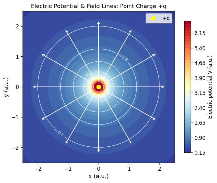
\[ \mathbf{E}(\mathbf{r}) = \frac{1}{4\pi\epsilon_0} \frac{q}{r^2}\, \mathbf{u}_r \]

where \(\mathbf{u}_r\) is the radial unit vector pointing away from the source. This is a central field with spherical symmetry: it points radially outward (for \(q > 0\)) and falls off as the square of the distance.

The field concept is more than a notational convenience. It is ontologically fundamental: when charges are in motion, the field carries energy and momentum. Disturbances propagate as electromagnetic waves. The field has physical reality independent of whether any test charge is present to feel it.

3.2 The Field of a Continuous Distribution

By the superposition principle, the field due to a continuous charge distribution with volume density \(\rho(\mathbf{r}')\) in a region \(\Omega\) is:

\[ \mathbf{E}(\mathbf{r}) = \frac{1}{4\pi\epsilon_0} \int_\Omega \rho(\mathbf{r}')\, \frac{\mathbf{r} - \mathbf{r}'}{|\mathbf{r} - \mathbf{r}'|^3}\, dV' \]

This integral, while conceptually straightforward, is in practice a vector integral that is hard to compute directly. The strategy is to break the source into infinitesimal pieces \(dq = \rho\, dV\), treat each piece as a point charge, compute its infinitesimal field contribution \(d\mathbf{E}\), and integrate.

A crucial step is the physics of the infinitesimal: we must convince ourselves that an infinitesimally small volume element \(dV\) carrying charge \(dq = \rho\, dV\) genuinely behaves as a point charge at the observer’s location. This requires only that the observation point \(P\) is at a distance much larger than the linear size of \(dV\) — which is guaranteed as \(dV \to 0\). The subtlety arises only when \(P\) approaches the source region itself, but for bounded, continuous \(\rho\), the integral converges even at source points.

3.3 Worked Examples

Infinite line of charge. Consider an infinite straight wire carrying uniform linear charge density \(\lambda\). By symmetry, the field must point radially away from the wire (for \(\lambda > 0\)) and its magnitude depends only on the perpendicular distance \(s\) from the wire. Setting up a cylindrical coordinate system with the \(z\)-axis along the wire and the field point at distance \(s\) in the \(xy\)-plane, each infinitesimal segment \(dz'\) at position \(z'\) contributes a field pointing from \((0, 0, z')\) toward \((s, 0, 0)\). By symmetry, the \(z\)-components from symmetric pairs cancel. Integrating the radial component:

\[ E = \frac{\lambda}{2\pi\epsilon_0 s}, \qquad \mathbf{E} = \frac{\lambda}{2\pi\epsilon_0 s}\, \mathbf{u}_s \]

The irrotational and Gauss properties of \(\mathbf{E}\) provide a more elegant derivation, as we shall see.

Infinite plane of charge. An infinite plane carrying uniform surface charge density \(\sigma\) has, by symmetry, a field that points perpendicularly away from the plane and depends only on which side you are on. Using either direct integration or Gauss’s theorem:

\[ \mathbf{E} = \frac{\sigma}{2\epsilon_0}\, \mathbf{n} \]

where \(\mathbf{n}\) is the outward unit normal. Remarkably, this is independent of distance from the plane — the field is uniform. Two parallel planes of opposite charge density, like a parallel-plate capacitor, produce a uniform field \(\sigma/\epsilon_0\) between them and (nearly) zero field outside.

Charged circular loop. For a loop of radius \(R\) carrying charge \(Q\), the field at a point on the axis at distance \(z\) from the centre has only a \(z\)-component (by symmetry, all transverse contributions cancel):

\[ E_z = \frac{1}{4\pi\epsilon_0} \frac{Qz}{(z^2 + R^2)^{3/2}} \]

This goes to zero at \(z = 0\) (the centre, where everything cancels) and at \(z \to \infty\), with a maximum at \(z = R/\sqrt{2}\).

---

Chapter 4: Gauss’s Theorem and the Irrotational Property

4.1 Gauss’s Theorem

The brute-force integration of Coulomb’s law is unwieldy for all but the simplest geometries. Gauss’s theorem provides a powerful alternative, trading a complex integral over the source for a simpler integral over any closed surface surrounding it.

The key insight is that the flux of \(\mathbf{E}\) through any closed surface depends only on the total charge enclosed, not on the shape of the surface. To prove this, consider first a single point charge \(q\) at the centre of a sphere of radius \(R\). The flux through the sphere is:

\[ \Phi = \oint_\Sigma \mathbf{E} \cdot \mathbf{n}\, dA = \frac{1}{4\pi\epsilon_0} \frac{q}{R^2} \cdot 4\pi R^2 = \frac{q}{\epsilon_0} \]

The factors of \(R^2\) cancel exactly — this is no accident but a direct consequence of the inverse-square law.

To generalise to an arbitrary closed surface \(\tilde\Sigma\), consider a cone of solid angle \(d\Omega\) emanating from \(q\). This cone intersects the sphere in an area element \(dA\) and the arbitrary surface in a tilted area element \(d\tilde A\). The projection of \(d\tilde A\) onto the radial direction is \(d\tilde A \cos\theta\), while the areas are related by \(dA' / dA = (r')^2/r^2\) (the ratio of their squared distances from \(q\)). When computing the flux through \(d\tilde A\), both the factor \(\cos\theta\) and the ratio of areas conspire to give exactly the same contribution as through \(dA\). The flux through any surface enclosing \(q\) equals \(q/\epsilon_0\).

By the superposition principle, for \(N\) point charges:

This is the first Maxwell equation for the electrostatic field. We have derived it from empirical laws — Coulomb and superposition — so it encodes exactly the same physics, merely repackaged.

Gauss’s theorem is powerful but insufficient alone. To determine \(\mathbf{E}\) uniquely from its flux through a surface, we need additional constraints — specifically, symmetry arguments or the second Maxwell equation, the irrotational property. The right-hand side of Gauss’s theorem (the enclosed charge integral) is easy to compute; the left-hand side involves \(\mathbf{E}\), which we are trying to find. Only when symmetry constrains the direction and position-dependence of \(\mathbf{E}\) can we extract \(|\mathbf{E}|\) from the flux integral.

Recovering the infinite-line result. For the infinite line, cylindrical symmetry demands \(\mathbf{E} = E(s)\, \mathbf{u}_s\). Draw a cylindrical Gaussian surface of radius \(s\) and length \(L\) coaxially around the wire. The flux through the end caps is zero (by symmetry, \(\mathbf{E} \perp\) end caps); through the cylindrical surface it is \(E \cdot 2\pi s L\). Gauss gives \(E \cdot 2\pi s L = \lambda L/\epsilon_0\), hence \(E = \lambda/(2\pi\epsilon_0 s)\) — in perfect agreement with the direct calculation.

4.2 The Irrotational Property of E

The second Maxwell equation for the electrostatic field is the irrotational property: the circulation of \(\mathbf{E}\) around any closed path is zero.

This follows from the inverse-square nature of Coulomb’s law. For a single point charge, \(\mathbf{E}\) is a central force field with a potential, and the work done along any closed loop in a potential field is zero — the potential is single-valued. By superposition, the sum of central fields also has zero circulation.

The irrotational property is not merely a technical result. It embodies the conservative nature of the electrostatic field: the work done moving a test charge depends only on the endpoints, not the path. This is what permits the definition of the electrostatic potential \(V\), discussed in the next chapter.

In the hierarchy of the two Maxwell equations for \(\mathbf{E}\), the irrotational property is arguably more fundamental. To fully determine \(\mathbf{E}\) from a given charge distribution, one typically needs both symmetry arguments (which encode information equivalent to the irrotational property) and Gauss’s theorem. The irrotational property constrains the tangential behaviour of \(\mathbf{E}\); Gauss’s theorem constrains the normal behaviour.

4.3 Local Form of Maxwell’s Equations: Case 1

The integral forms are most general, but for regions where \(\rho\) is continuous and bounded, we can pass to differential (local) forms using the divergence theorem and Stokes’ theorem.

The divergence theorem converts \(\oint_{\tilde\Sigma} \mathbf{E} \cdot \mathbf{n}\, dA = \int_{\tilde\Omega} \nabla \cdot \mathbf{E}\, dV\), and comparing with \(\int \rho/\epsilon_0\, dV\) gives \(\nabla \cdot \mathbf{E} = \rho/\epsilon_0\). Similarly, Stokes’ theorem converts \(\oint_\Gamma \mathbf{E} \cdot \mathbf{t}\, dl = \int_{\Sigma_\Gamma} (\nabla \times \mathbf{E}) \cdot \mathbf{n}\, dA = 0\), giving \(\nabla \times \mathbf{E} = \mathbf{0}\) (in a simply connected domain).

Case 1 requires that \(\rho\) be continuous — it fails at surfaces carrying \(\sigma\). When surface charges are present, we need the local form for Case 2.

4.4 Local Form: Case 2 — Boundary Conditions

When charge is concentrated on a surface \(\Sigma\) with surface density \(\sigma\), the volume density \(\rho\) is not continuous across \(\Sigma\). In this regime, the differential form breaks down and must be replaced by boundary conditions that relate field values on the two sides of the surface.

Label the two sides as region 1 (above \(\Sigma\)) and region 2 (below), with the unit normal \(\mathbf{n}_{21}\) pointing from region 2 to region 1.

The normal component of \(\mathbf{E}\) is discontinuous across a charged surface — the discontinuity equals \(\sigma/\epsilon_0\). The tangential component is continuous. These boundary conditions are the working tools for problems involving surfaces.

The classic example is the infinite conducting plane (at equilibrium, to be discussed in Chapter 9): the field just outside the conductor is \(\sigma/\epsilon_0\), perpendicular to the surface, and the field inside is zero.

There is also a Case 3 — the exterior of a finite charged object where charge resides only on the boundary and nothing exists inside (a spherical shell, for instance). Here, the field outside is determined by Gauss and irrotational, while inside the shell the field vanishes by the superposition of contributions from all parts of the shell.

---

Chapter 5: The Electrostatic Potential

5.1 From Field to Potential

The irrotational property \(\nabla \times \mathbf{E} = \mathbf{0}\) has a deep consequence: in any simply connected domain, an irrotational field is necessarily conservative and can be written as the gradient of a scalar function.

The move from \(\mathbf{E}\) (a vector with three components) to \(V\) (a scalar with one) is not just algebraic economy — it reflects a deep physical simplification. The gradient of \(V\) recovers \(\mathbf{E}\) completely, losing no information, while reducing a vector problem to a scalar problem.

The mountain analogy is instructive. The gradient of a surface’s height function points in the direction of steepest ascent; minus the gradient points in the direction of steepest descent. A test charge in an electric field is like a ball on a landscape: it “rolls downhill” in \(V\) (for positive test charges). The sign convention ensures this analogy works cleanly with gravity.

5.2 Potential of a Point Charge

For a single point charge \(q\) at the origin, the field is radial: \(\mathbf{E} = (q/4\pi\epsilon_0 r^2)\,\mathbf{u}_r\). In spherical coordinates, the gradient of a function that depends only on \(r\) is \(\nabla V = (dV/dr)\,\mathbf{u}_r\). Setting \(-dV/dr = q/(4\pi\epsilon_0 r^2)\) and integrating:

\[ V(r) = \frac{1}{4\pi\epsilon_0} \frac{q}{r} + C \]

The constant of integration \(C\) is arbitrary and represents our freedom to choose a reference point for potential. The standard convention — zero potential at infinity — sets \(C = 0\):

\[ V(r) = \frac{1}{4\pi\epsilon_0} \frac{q}{r} \]

This is the Green’s function for the Laplace/Poisson operator in free space. With zero potential at infinity, the potential of any bounded charge distribution also vanishes at infinity. The convention fails only for unbounded distributions (infinite line, infinite plane), which require a finite reference point.

5.3 Potential of Continuous Distributions

By superposition:

\[ V(\mathbf{r}) = \frac{1}{4\pi\epsilon_0} \int_\Omega \frac{\rho(\mathbf{r}')}{|\mathbf{r} - \mathbf{r}'|}\, dV' \]

This scalar integral is considerably easier to compute than the vector integral for \(\mathbf{E}\). One first computes \(V\), then recovers \(\mathbf{E} = -\nabla V\). The strategy is particularly effective for problems with moderate symmetry where the direct evaluation of \(\nabla V\) is still manageable.

5.4 Properties of V and Relations to E

The potential of a spherical shell of charge \(Q\) and radius \(R\) is, outside the shell (\(r > R\)): \(V = Q/(4\pi\epsilon_0 r)\), identical to a point charge at the centre. Inside (\(r < R\)) the potential is constant: \(V = Q/(4\pi\epsilon_0 R)\). This constancy inside is remarkable — it means \(\mathbf{E} = -\nabla V = \mathbf{0}\) inside the shell. An infinitely charged thin shell produces no net field in its interior.

For the infinite charged line (charge density \(\lambda\)), the potential cannot be taken to zero at infinity (since the distribution is unbounded). Choosing the reference point at a finite distance \(s_0\):

\[ V(s) = -\frac{\lambda}{2\pi\epsilon_0} \ln\!\left(\frac{s}{s_0}\right) \]

Differentiating: \(E_s = -\partial V/\partial s = \lambda/(2\pi\epsilon_0 s)\), recovering the known result.

For a uniformly charged sphere of total charge \(Q\) and radius \(R\):

• Outside (\(r > R\)): \(V = Q/(4\pi\epsilon_0 r)\)
• Inside (\(r < R\)): \(V = Q/(4\pi\epsilon_0)\cdot(3R^2 - r^2)/(2R^3)\)

The interior potential is determined by integrating \(\mathbf{E} = -\nabla V\) inward from the surface, using the interior field found from Gauss’s theorem.

5.5 Poisson and Laplace Equations

Combining \(\mathbf{E} = -\nabla V\) with the Gauss equation \(\nabla \cdot \mathbf{E} = \rho/\epsilon_0\), we obtain:

\[ \nabla \cdot (-\nabla V) = \frac{\rho}{\epsilon_0} \]

The operator \(\nabla \cdot \nabla = \nabla^2\) is the scalar Laplacian, yielding the Poisson equation:

When \(\rho = 0\) (charge-free region), it reduces to the Laplace equation:

In a Cartesian coordinate system:

\[ \nabla^2 V = \frac{\partial^2 V}{\partial x^2} + \frac{\partial^2 V}{\partial y^2} + \frac{\partial^2 V}{\partial z^2} = 0 \]

Laplace’s equation is indispensable: it governs the electrostatic potential everywhere outside a charge distribution. To find \(V\) in a conductor-bounded region, we solve Laplace’s equation in the vacuum subject to boundary conditions on the conducting surfaces. This is the Dirichlet problem — finding a harmonic function with specified boundary values. The solution is unique, guaranteeing that specifying the potentials of all conductors in a system completely determines the field.

---

Chapter 6: Electrostatic Energy

6.1 Energy of Discrete Charge Configurations

The electrostatic energy of a charge configuration is the total work required to assemble it by bringing charges in from infinity one by one. For two point charges \(q_1\) and \(q_2\) separated by distance \(r_{12}\):

\[ U = \frac{1}{4\pi\epsilon_0} \frac{q_1 q_2}{r_{12}} \]

The interpretation: this is the work done by an external agent (or the work done against the electrostatic force) to bring \(q_2\) from infinity to its current position in the field of \(q_1\). When \(q_1 q_2 > 0\) (like charges), \(U > 0\): we must do positive work against repulsion. When \(q_1 q_2 < 0\), \(U < 0\): the particles attract and release energy as they approach.

For \(N\) point charges, the total energy is:

\[ U_E = \frac{1}{2} \sum_{i=1}^N q_i V_i \]

where \(V_i\) is the potential at the location of charge \(i\) due to all other charges. The factor of \(1/2\) corrects for double-counting: each pair \((i, j)\) would otherwise appear twice in the sum (once as the work to bring \(q_j\) into the field of \(q_i\), and once for the reverse).

6.2 Energy of Continuous Distributions

For a continuous charge distribution \(\rho\) in a region \(\Omega\), the sum becomes an integral. The conceptual procedure mirrors the discrete case: partition \(\Omega\) into infinitesimal volume elements, each carrying charge \(dq = \rho\, dV\) and each behaving as a point charge. Spread all these charges to infinity, then reassemble them in their original positions:

\[ U_E = \frac{1}{2} \int_\Omega \rho(\mathbf{r})\, V(\mathbf{r})\, dV \]

The integral can be extended to all space (since \(\rho = 0\) outside \(\Omega\), those regions contribute nothing). This electrostatic energy is the “glue” holding the charge distribution together — it is the energy stored in the electric field configuration.

6.3 Energy in Terms of the Field

There is an alternative, and deeply illuminating, expression for the electrostatic energy entirely in terms of \(\mathbf{E}\) rather than \(\rho\) and \(V\). Substituting \(\rho = \epsilon_0 \nabla \cdot \mathbf{E}\) and integrating by parts:

\[ U_E = \frac{\epsilon_0}{2} \int_{\text{all space}} |\mathbf{E}|^2\, dV \]

This result says the energy is stored in the field itself, not in the charges. The energy density of the electric field is:

\[ u_E = \frac{\epsilon_0}{2} E^2 \]

This perspective — energy residing in fields rather than in particles — becomes essential in electromagnetic radiation, where energy propagates through empty space as oscillating electric and magnetic fields long after the source charges have been turned off.

6.4 Energy Caveats

The expression \(U_E = \frac{1}{2}\int \rho V\, dV\) contains a subtlety when applied to point charges: the potential \(V\) diverges at the location of each point charge, making the self-energy of a point charge formally infinite. This divergence is a fundamental problem of classical electrodynamics that is resolved (partially) only in quantum electrodynamics. In practice, when computing interaction energies between well-separated charge distributions, the self-energy contributions are treated as constants that cancel out.

For extended charge distributions — spheres, shells, plates — the self-energy is finite and physically meaningful. For example, the energy stored in a uniformly charged sphere of radius \(R\) and total charge \(Q\) is:

\[ U_E = \frac{3}{5} \frac{Q^2}{4\pi\epsilon_0 R} \]

This can be computed using \(\int \rho V\, dV\), integrating over the sphere. Alternatively, assembling the sphere shell by shell and computing the work against the field already present reproduces the same result.

6.5 The Dirac Delta Function

The Dirac delta function \(\delta(\mathbf{r} - \mathbf{r}')\) is an indispensable tool for bridging discrete and continuous descriptions. Informally, it is the limit of an infinitely tall, infinitely narrow peak of unit area centred at \(\mathbf{r}'\):

\[ \delta(\mathbf{r} - \mathbf{r}') = 0 \quad (\mathbf{r} \neq \mathbf{r}'), \qquad \int \delta(\mathbf{r} - \mathbf{r}')\, dV = 1 \]

Its key property is the sifting property: \(\int f(\mathbf{r})\, \delta(\mathbf{r} - \mathbf{r}')\, dV = f(\mathbf{r}')\). A point charge \(q\) at \(\mathbf{r}'\) is represented as the continuous density \(\rho(\mathbf{r}) = q\, \delta(\mathbf{r} - \mathbf{r}')\). The Laplacian of the Coulomb potential is:

\[ \nabla^2 \!\left(\frac{1}{r}\right) = -4\pi\, \delta(\mathbf{r}) \]

a central identity used throughout field theory. It resolves the apparent paradox that \(\nabla^2 (1/r) = 0\) everywhere except the origin, while the total flux from a unit charge must equal \(1/\epsilon_0\) — the delta function supplies the missing source at the origin.

---

Chapter 7: Conductors in Electrostatic Equilibrium

7.1 The Microscopic Picture: Fermi Water Model

A conductor is a material that contains free charge carriers — in metals, these are the conduction electrons (one or more per atom). These electrons are not bound to any particular ion but move freely through the crystal lattice. The lattice provides a background of positive ions. At zero temperature, the electrons fill all available quantum states up to the Fermi energy — a concept described by the Fermi-Dirac distribution. At room temperature, only electrons near the Fermi surface are thermally excited.

For our purposes, the essential point is simpler: there exists a large density of charge carriers that can respond almost instantaneously to any applied electric field. The timescale for this response — the relaxation time of a conductor — is on the order of \(10^{-18}\) seconds (femtoseconds) for good conductors like copper or aluminium. After this transient, the system reaches macroscopic electrostatic equilibrium.

At the microscopic level, the positive ions form a periodic lattice structure (visualised as fixed, immovable), while the conduction electrons constitute a “sea” that moves. When an external field \(\mathbf{E}_X\) is applied, the electrons are displaced against the field (since they carry negative charge), creating a reaction field \(\mathbf{E}_R\) that opposes \(\mathbf{E}_X\). This is the Helmholtz double layer: a thin layer of negative charge on one surface and positive charge (ion depletion) on the opposite surface.

7.2 Macroscopic Electrostatic Equilibrium

After the transient, the conductor reaches macroscopic electrostatic equilibrium (MEE). This condition has a remarkably clean characterisation:

The proof rests on the impossibility of perpetual motion. The reaction field \(\mathbf{E}_R\) builds up during the transient as electrons accumulate on surfaces. Conservation of energy demands that \(\mathbf{E}_R\) cannot exceed \(\mathbf{E}_X\) — if it did, electrons would continue accelerating indefinitely, violating energy conservation. Equilibrium is reached precisely when \(\mathbf{E}_R = -\mathbf{E}_X\), making the total interior field zero.

A tennis ball analogy makes this vivid. Imagine positive ions as orange balls fixed in a box, and electrons as free blue balls. Open the box lid and gravity pulls the free balls to the bottom — they redistribute until every ball is resting in a potential minimum. After the settling, no ball moves: the net force on each is zero. In the conductor, the equilibrium condition is \(m_e a = e(\mathbf{E}_X + \mathbf{E}_R) = 0\).

Several profound consequences follow from MEE:

1. Interior field is zero: \(\mathbf{E} = 0\) throughout the bulk.
2. Charge resides on the surface: by Gauss’s law applied to a surface just inside the conductor surface, all free charge must reside on the outer skin \(\Sigma\).
3. Surface is an equipotential: since \(\mathbf{E} = 0\) inside, \(V\) is constant throughout the conductor (including its surface).
4. External field is normal: at the conductor surface, \(\mathbf{E}\) must be perpendicular to the surface (since any tangential component would drive a current and the system would not be in equilibrium).

A conductor with infinite conductivity is a perfect conductor. It expels all electric fields from its interior. Interestingly, a superconductor does the analogous thing for magnetic fields — it expels \(\mathbf{B}\) from its interior (the Meissner effect). Perfect conductors shield against electric fields; superconductors shield against magnetic fields.

7.3 Coulomb’s Theorem

The condition \(\mathbf{E} = 0\) inside a conductor, combined with the boundary condition for a surface charge, determines the external field just outside the surface.

The derivation uses the boundary condition for the normal component: \(E_{1,n} - E_{2,n} = \sigma/\epsilon_0\). With \(\mathbf{E}_2 = 0\) (inside the conductor), we immediately get \(E_{1,n} = \sigma/\epsilon_0\).

Coulomb’s theorem also provides a computational tool: given the electrostatic potential \(V\) outside the conductor (a solution to Laplace’s equation satisfying the boundary conditions), the surface charge density is:

\[ \sigma = -\epsilon_0 \left.\frac{\partial V}{\partial n}\right|_{\Sigma^+} \]

where the derivative is taken just outside the surface \(\Sigma\), approaching from the vacuum side.

7.4 Electrostatic Shielding

One of the most practically important consequences of conductors is electrostatic shielding: a closed conducting shell shields its interior from any external electric field. The argument is straightforward — at equilibrium, the field inside any closed conducting shell is zero regardless of what fields exist outside. Faraday cages exploit this principle. Electronics, sensitive instruments, and military hardware are often housed in conducting enclosures to protect them from external electromagnetic interference.

The shielding is not perfect in the sense that it takes a finite transient time to establish, but for the steady-state (DC) case and for slowly varying fields where the relaxation time is short compared to the field variation timescale, it is essentially perfect.

7.5 The External Dirichlet Problem

In many situations, we know the potential on all conducting surfaces and want to find \(V\) everywhere in the surrounding vacuum. This is the external Dirichlet problem: find a harmonic function \(V\) (satisfying Laplace’s equation) in the exterior region, subject to specified boundary values on the conductors and the condition \(V \to 0\) at infinity.

The fundamental result is that the Dirichlet problem has a unique solution. This uniqueness theorem underpins all of electrostatics: once you specify the charge on each conductor (or equivalently the potential on each conductor surface), the field everywhere is completely determined. There is only one field configuration consistent with the given boundary conditions.

For a conducting sphere of radius \(R\) carrying charge \(Q\), the potential outside is \(V = Q/(4\pi\epsilon_0 r)\), and the surface charge density is uniform: \(\sigma = Q/(4\pi R^2)\). The field outside is that of a point charge at the centre — a beautiful result proved by Gauss’s theorem and the spherical symmetry.

---

Chapter 8: Capacitors

8.1 Capacitance of a Single Conductor

The concept of capacitance emerges naturally from the harmonic properties of the electrostatic potential. Consider a single isolated conductor \(\Gamma\) with outer surface \(\Sigma\). If we apply charge \(Q_1\) to it, Laplace’s equation in the exterior vacuum (with appropriate boundary conditions) gives a potential \(V_1(P)\) at any exterior point \(P\). If instead we apply charge \(Q_2\), we get \(V_2(P)\). Since Laplace’s equation is linear, \(V_2 \propto Q_2\) and \(V_1 \propto Q_1\), and hence \(V_2/V_1\) is the constant ratio \(Q_2/Q_1\) independent of position. Equivalently:

\[ \frac{Q_1}{V_1} = \frac{Q_2}{V_2} = \cdots = C \]

This universal constant, the ratio of charge to potential, is the capacitance:

The capacitance is an intrinsic geometric property of the conductor — it depends on the conductor’s shape and size but not on how much charge is placed on it. The analogy with mass (force = mass × acceleration) is exact in structure: capacitance is to the charge-potential relationship what mass is to the force-acceleration relationship. One farad is an enormous capacitance in practice; typical values range from picofarads (\(10^{-12}\,\text{F}\)) in electronic circuits down to attofarads (\(10^{-18}\,\text{F}\)) in nanoscale devices such as superconducting qubits.

For a conducting sphere of radius \(R\):

\[ C_\text{sphere} = 4\pi\epsilon_0 R \]

Setting \(R = 1\,\text{m}\) gives \(C \approx 111\,\text{pF}\) — consistent with the size of the Earth.

8.2 Two-Conductor Capacitors

In most practical applications, a capacitor consists of two conductors. The parallel-plate capacitor is the archetype: two large flat conducting plates of area \(A\) separated by a gap \(d\). By the boundary conditions and Gauss’s theorem, the field between the plates is uniform: \(E = \sigma/\epsilon_0 = Q/(\epsilon_0 A)\). The potential difference across the gap is:

\[ \Delta V = E \cdot d = \frac{Qd}{\epsilon_0 A} \]

The capacitance is:

\[ C = \frac{Q}{\Delta V} = \frac{\epsilon_0 A}{d} \]

This result reveals the three geometric levers: increasing plate area or decreasing separation increases \(C\), while an interposed dielectric (not covered in PHYS 242, but treated in 342) multiplies \(C\) by the dielectric constant.

\[ \frac{1}{C_\text{tot}} = \frac{1}{C_1} + \frac{1}{C_2} \]\[ C_\text{tot} = C_1 + C_2 \]

8.3 Grounding and Dynamic Charge

Grounding a conductor connects it to a reservoir at fixed potential (conventionally \(V = 0\)). When a grounded conductor is brought near a charged object, charge flows to or from ground to maintain \(V = 0\). Grounding provides an infinite reservoir of charge and is the physical meaning of the “zero potential at infinity” boundary condition.

When a charged conductor suddenly connects to another conductor (or to ground), the system is abruptly thrown out of macroscopic electrostatic equilibrium. During the resulting transient, charge flows, an electric current exists, and only after a very short time (the relaxation time \(\sim 10^{-18}\,\text{s}\) for copper) does the new equilibrium establish itself. This dynamic charge scenario is the bridge between electrostatics and the study of currents.

---

Part II: Electric Currents

Chapter 9: The Magnetic Field and the Lorentz Force

9.1 When Charges Move

Everything done in Part I assumed the source charges to be at rest in an inertial reference frame. When charges move, new phenomena emerge. The definitive empirical summary is the Lorentz force law:

The Lorentz force summarises a fourfold classification depending on whether the source charges and the test charge are at rest or moving:

Source charges	Test charge	Force at \(P\)
At rest (\(\mathbf{v}_Q = 0\))	At rest (\(\mathbf{v}_P = 0\))	\(q_0 \mathbf{E}\) — electrostatics
At rest	Moving	\(q_0 \mathbf{E}\) — same field, no magnetic effect
Moving (\(\mathbf{v}_Q \neq 0\))	At rest	\(q_0 \mathbf{E}(\mathbf{r},t)\) — dynamic field, no detectable \(\mathbf{B}\)
Moving	Moving	\(q_0(\mathbf{E} + \mathbf{v}_P \times \mathbf{B})\) — full Lorentz force

This table reveals that a magnetic field is generated whenever charges are moving, but it can only be detected by a moving test charge. A test charge at rest is completely insensitive to the magnetic field — there is no magnetic monopole analogue to the electric force on a static charge.

The name “Lorentz force” honours Hendrik Antoon Lorentz, who synthesised 19th-century results into this compact form. It can also be derived from first principles using the principle of least action (the Lagrangian approach), but the empirical route is more transparent for an introductory course.

9.2 Measuring the Magnetic Field

The magnitude and direction of \(\mathbf{B}\) at a point can be determined experimentally by measuring the force on a moving test charge. One fires a known charge \(q_0\) with known velocity \(\mathbf{v}_P\) through the point and measures the resultant force. Since \(\mathbf{E}\) is separately measurable (by the force on a static charge), the magnetic contribution \(q_0 \mathbf{v}_P \times \mathbf{B}\) can be isolated. The SI unit of \(\mathbf{B}\) is the tesla (\(\text{T} = \text{kg}\,\text{A}^{-1}\,\text{s}^{-2}\)).

---

Chapter 10: Electric Currents

10.1 Current Intensity

An electric current is a flow of charge. The current intensity \(I\) through a surface \(\Sigma\) is the net charge crossing \(\Sigma\) per unit time:

\[ I = \frac{dQ}{dt} \]

More precisely, since charge carriers can cross in either direction, \(I\) is the net rate: positive charge flowing in one direction minus negative charge (electrons) flowing in the opposite direction contribute additively. In a conductor, the relevant charge carriers are the conduction electrons; \(I > 0\) by convention corresponds to net positive charge flow.

The SI unit is the ampere (A = C/s).

10.2 Drift and Diffusion

At finite temperature, conduction electrons in a metal move with large thermal velocities (on the order of \(10^6\,\text{m/s}\) for copper at room temperature), but in random directions — no net current. When an electric field \(\mathbf{E}\) is applied, it superimposes a small drift velocity \(\mathbf{v}_d\) on the thermal motion. For typical household currents, \(|\mathbf{v}_d| \sim 10^{-4}\,\text{m/s}\) — remarkably slow compared to thermal velocities.

The drift-diffusion model describes this in the Lagrangian framework: following individual electron trajectories. The complementary Eulerian framework describes the field of velocities at fixed points in space. Both perspectives are useful; the Eulerian description directly connects to the macroscopic current density.

10.3 Current Density Vector

The current density vector \(\mathbf{J}\) is the microscopic, local version of current intensity:

The current intensity through a surface \(\Sigma\) is recovered as the flux of \(\mathbf{J}\):

\[ I = \int_\Sigma \mathbf{J} \cdot \mathbf{n}\, dA \]

For a quasi-filiform (thin) conductor aligned with direction \(\mathbf{t}\), \(\mathbf{J} = J\, \mathbf{t}\) and \(I = J \Delta A\), where \(\Delta A\) is the cross-sectional area.

10.4 The Continuity Equation

Charge conservation — the most fundamental law in electromagnetism — takes the form of the continuity equation. Consider a conductor \(\Omega\) bounded by surface \(\Sigma\). Charge conservation states that any increase in charge within \(\Omega\) must be due to a net inflow through \(\Sigma\):

\[ \frac{dQ}{dt} = -\oint_\Sigma \mathbf{J} \cdot \mathbf{n}\, dA \]

(The minus sign: outward \(\mathbf{n}\) means positive flux corresponds to charge leaving.) Applying the divergence theorem to the right side:

\[ \frac{d}{dt}\int_\Omega \rho_c\, dV = -\int_\Omega \nabla \cdot \mathbf{J}\, dV \]

Since \(\Omega\) is fixed (not moving), the time derivative can enter under the integral:

For stationary currents — the steady state where charge densities do not change in time — \(\partial \rho_c/\partial t = 0\) and the continuity equation reduces to \(\nabla \cdot \mathbf{J} = 0\): \(\mathbf{J}\) is solenoidal (divergence-free). Solenoidal fields have closed field lines — exactly the statement that steady currents must flow in closed loops.

10.5 Stationary Currents and Flux Tubes

A stationary current satisfies \(\nabla \cdot \mathbf{J} = 0\), \(\nabla \times \mathbf{B} = \mu_0 \mathbf{J}\), and the boundary condition that \(\mathbf{J} \cdot \mathbf{n} = 0\) at the conductor surface (no current leaves sideways). The flux tube is a conceptual tool: a tube whose walls follow field lines of \(\mathbf{J}\). Since no \(\mathbf{J}\) crosses the walls, the current intensity through any cross-section of the tube is constant. This is the microscopic basis of Kirchhoff’s current law.

10.6 Ohm’s Law and Joule’s Law

Ohm’s law in its local form relates the current density to the local electric field:

This linear relationship holds for many materials (ohmic or linear materials) over a wide range of field strengths. It breaks down for very large fields, non-uniform materials, nonlinear semiconductors, and superconductors.

The resistance of a wire of length \(L\) and cross-section \(A\) is \(R = \eta L/A = L/(\sigma_c A)\). The macroscopic Ohm’s law \(V = IR\) follows by integrating the local form along the wire.

Joule’s law gives the power dissipated per unit volume by an ohmic conductor:

Joule heating is irreversible — it converts ordered electrical energy into thermal energy. The Joule law is why incandescent bulbs glow and why power transmission lines are kept at high voltage (low current): at given power \(P = IV\), high \(V\) means low \(I\), reducing \(I^2 R\) losses.

---

Chapter 11: Electromotive Force and Batteries

11.1 Why E Alone Cannot Sustain a Current

A seemingly natural question: can a static electric field drive a permanent current? The answer is no. For a steady current, the current density \(\mathbf{J}\) must be solenoidal — its field lines must be closed loops. But the work done by \(\mathbf{E}\) around any closed loop is:

\[ W = q_0 \oint_\Gamma \mathbf{E} \cdot \mathbf{t}\, dl = 0 \]

by the irrotational property of \(\mathbf{E}\) (in steady conditions, even with moving charges creating a dynamic \(\mathbf{E}\), the irrotational property holds for conservative fields in simply connected domains). Zero work, zero net force around the loop — the charges would simply stop after any transient has dissipated.

For an ohmic conductor, this is explicit: integrating Ohm’s law around a closed loop of length \(L\) and uniform cross-section gives \(\eta_c J L = 0\) (since the circulation of \(\mathbf{E}\) is zero), forcing \(J = 0\).

What is needed is a non-conservative force — a force whose circulation around a closed loop is nonzero. Such a force can keep charges moving indefinitely without violating energy conservation, because energy is being supplied by the non-conservative mechanism (chemical energy in a battery, mechanical energy in a generator, light in a photovoltaic cell).

11.2 The Electromotive Force

A battery (or any source) provides this non-conservative force. At the microscopic level, electrochemical reactions push charge carriers from the negative terminal to the positive terminal against the electrostatic field. Macroscopically, we model this as a motional force \(\mathbf{F}_m\) confined within the battery region. The associated field inside the battery is:

\[ \mathbf{E}_m = \frac{\mathbf{F}_m}{q_0} \]

This field is non-zero only inside the battery — it is confined, unlike \(\mathbf{E}\) which extends everywhere. The electromotive force (EMF) is defined as the work done by \(\mathbf{E}_m\) on a unit positive charge traversing the battery from negative to positive terminal:

The EMF is non-zero precisely because \(\mathbf{E}_m\) is non-conservative: \(\oint_\Gamma \mathbf{E}_m \cdot \mathbf{t}\, dl = \mathcal{E} \neq 0\). Within the battery, \(\mathbf{E}_m\) and the conservative field \(\mathbf{E}\) both exist; outside the battery, only \(\mathbf{E}\) exists, pointing from the positive plate to the negative plate around the external circuit.

11.3 Ohm’s Law in Integral Form

For a closed circuit consisting of a battery with EMF \(\mathcal{E}\) and internal resistance \(r\) connected to an external resistance \(R\), the integral form of Ohm’s law gives:

\[ \mathcal{E} = I(R + r) \]

This is the macroscopic Kirchhoff voltage law. The current \(I = \mathcal{E}/(R + r)\). Special cases:

• Open circuit (\(R \to \infty\)): \(I = 0\), the terminal voltage equals \(\mathcal{E}\).
• Short circuit (\(R = 0\)): \(I = \mathcal{E}/r\), limited only by internal resistance.
• Loaded circuit: \(I = \mathcal{E}/(R + r)\), terminal voltage is \(V_\text{terminal} = IR = \mathcal{E} R/(R + r) < \mathcal{E}\).

11.4 Resistance of a Longitudinal Wire and Coaxial Cable

For a straight wire of length \(L\), cross-section \(A\), and resistivity \(\eta\):

\[ R = \frac{\eta L}{A} \]

For a coaxial cable — a central conductor of radius \(a\) inside an outer cylindrical shell of radius \(b\) — the resistance per unit length of the coaxial geometry must be computed by integrating over the annular cross-section if the current flows radially, or the simple \(\eta L/A\) formula applies if it flows longitudinally. In the transverse (leakage) direction, the resistance is:

\[ R_\perp = \frac{\eta}{2\pi L} \ln\!\left(\frac{b}{a}\right) \]

This dependence on \(\ln(b/a)\) is characteristic of cylindrical geometry, just as the potential of an infinite line charge depends on \(\ln r\).

11.5 Ponderomotive Forces

When a current-carrying conductor is placed in an external magnetic field, the conduction electrons experience the magnetic component of the Lorentz force \(\mathbf{J} \times \mathbf{B}\). This manifests as a macroscopic ponderomotive (or Ampere) force on the conductor:

\[ d\mathbf{F} = I\, d\mathbf{l} \times \mathbf{B} \]

for a filiform conductor segment \(d\mathbf{l}\) carrying current \(I\). Integrating over the length of the conductor gives the total force. This is the principle behind electric motors and actuators.

---

Part III: Magnetostatics

Chapter 12: Maxwell’s Equations for the Magnetostatic Field

12.1 The Solenoidal Property of B

The magnetic field has no sources (no magnetic monopoles have ever been observed). This is encoded in the solenoidal property of B:

This is the second Maxwell equation for \(\mathbf{B}\) (or more precisely, the Maxwell-Gauss equation for \(\mathbf{B}\)). It contrasts sharply with \(\nabla \cdot \mathbf{E} = \rho/\epsilon_0\) — while electric field lines begin on positive charges and end on negative charges, magnetic field lines are closed loops with no beginnings or ends.

12.2 Ampere’s Law

The analogue of the irrotational property for \(\mathbf{E}\) is, for \(\mathbf{B}\), the Ampere circuital law — but with a crucial sign difference: \(\mathbf{B}\) is not irrotational.

This law holds only in magnetostatics (steady currents). In electrodynamics, the right-hand side acquires an additional “displacement current” term, completing Maxwell’s equations. The modification is vital for electromagnetic waves.

The concept of linkage is topological: a current \(I\) carried by a wire is linked with a closed curve \(\Gamma\) if the wire passes through any surface bounded by \(\Gamma\) an odd number of times. The algebraic sign of \(I_\Gamma\) depends on orientation — if the current direction is consistent with the right-hand rule for \(\Gamma\), it contributes positively; otherwise negatively.

The differential form follows from Stokes’ theorem:

\[ \nabla \times \mathbf{B} = \mu_0 \mathbf{J} \]

Compare this with \(\nabla \times \mathbf{E} = \mathbf{0}\) — the current density \(\mathbf{J}\) acts as the “source” of the curl of \(\mathbf{B}\), just as \(\rho\) acts as the source of the divergence of \(\mathbf{E}\).

Ampere’s law requires a simply connected domain for the equivalence between integral and differential forms to hold. A multiply connected domain — one with a hole through which a current passes — requires special care: the field might appear irrotational in a restricted region while having a non-trivial circulation around the hole (just as \(\oint d\theta = 2\pi\) around the origin even though \(\nabla \theta\) is defined away from the origin).

12.3 Applying Ampere’s Law: Infinite Line of Current

For an infinite straight wire carrying current \(I\), the symmetry of the problem demands that \(\mathbf{B}\) circles the wire in the azimuthal direction \(\mathbf{u}_\phi\) and depends only on the radial distance \(s\) from the wire. Choosing \(\Gamma\) to be a circle of radius \(s\) coaxial with the wire:

\[ \oint_\Gamma \mathbf{B} \cdot \mathbf{t}\, dl = B \cdot 2\pi s = \mu_0 I \]\[ \mathbf{B} = \frac{\mu_0 I}{2\pi s}\, \mathbf{u}_\phi \]

The field decreases as \(1/s\) — identical in form to the electric field of an infinite line charge \(\lambda/(2\pi\epsilon_0 s)\), with the replacement \(\lambda/\epsilon_0 \leftrightarrow \mu_0 I\). The field lines are concentric circles around the wire, following the right-hand rule.

12.4 Boundary Conditions for B

Analogously to the electric case, the Maxwell equations for \(\mathbf{B}\) impose boundary conditions at a surface carrying a surface current density \(\mathbf{K}\) (A/m):

\[ (\mathbf{B}_1 - \mathbf{B}_2) \cdot \mathbf{n}_{21} = 0 \qquad \text{(normal component, continuous)} \]\[ (\mathbf{B}_1 - \mathbf{B}_2) \times \mathbf{n}_{21} = \mu_0 \mathbf{K} \qquad \text{(tangential component, discontinuous)} \]

The normal component of \(\mathbf{B}\) is always continuous (reflecting \(\nabla \cdot \mathbf{B} = 0\)); the tangential component is discontinuous by \(\mu_0 \mathbf{K}\).

---

Chapter 13: The Vector Potential and Biot-Savart Law

13.1 The Vector Potential

Since \(\nabla \cdot \mathbf{B} = 0\), the magnetic field is solenoidal. By the Helmholtz theorem, any solenoidal field can be written as the curl of another vector field:

The vector potential is the magnetic analogue of the scalar potential \(V\) for \(\mathbf{E}\). The analogy is asymmetric: \(V\) is a scalar while \(\mathbf{A}\) is a vector, reflecting the richer topology of magnetic fields.

The vector potential is not unique: if \(\mathbf{B} = \nabla \times \mathbf{A}\), then \(\mathbf{A}' = \mathbf{A} + \nabla \psi\) for any scalar function \(\psi\) also satisfies \(\nabla \times \mathbf{A}' = \mathbf{B}\) (since \(\nabla \times \nabla \psi = \mathbf{0}\) identically). This gauge freedom — the ability to change \(\mathbf{A}\) without changing \(\mathbf{B}\) — is a deep structural feature. Among the infinite family of valid vector potentials, we can always choose one with \(\nabla \cdot \mathbf{A} = 0\) (Coulomb gauge). This choice, which sets the divergence of \(\mathbf{A}\) to zero, simplifies the equation for \(\mathbf{A}\) considerably.

In the Coulomb gauge, the combination of \(\mathbf{B} = \nabla \times \mathbf{A}\) with \(\nabla \times \mathbf{B} = \mu_0 \mathbf{J}\) gives:

\[ \nabla^2 \mathbf{A} = -\mu_0 \mathbf{J} \]

This is the vector Poisson equation — three separate scalar Poisson equations, one for each component of \(\mathbf{A}\). By analogy with the scalar case, the solution is:

\[ \mathbf{A}(\mathbf{r}) = \frac{\mu_0}{4\pi} \int_\Omega \frac{\mathbf{J}(\mathbf{r}')}{|\mathbf{r} - \mathbf{r}'|}\, dV' \]

The vector potential decays as \(1/r\) at large distances, just like the scalar potential.

13.2 Magnetic Flux via the Vector Potential

The magnetic flux through an open surface \(\Sigma_\Gamma\) bounded by a closed curve \(\Gamma\) is:

\[ \Phi = \int_{\Sigma_\Gamma} \mathbf{B} \cdot \mathbf{n}\, dA = \int_{\Sigma_\Gamma} (\nabla \times \mathbf{A}) \cdot \mathbf{n}\, dA \]

By Stokes’ theorem, this transforms to a line integral around the boundary:

\[ \Phi = \oint_\Gamma \mathbf{A} \cdot \mathbf{t}\, dl \]

This is a remarkable result: the magnetic flux through any surface bounded by \(\Gamma\) is independent of which surface we choose — it depends only on the bounding curve \(\Gamma\). This topological invariance underlies the concept of gauge invariance and has deep consequences in quantum mechanics (the Aharonov-Bohm effect) and in superconductivity, where the gauge-invariant phase of the Cooper pair condensate is related to the vector potential integral around a loop.

13.3 The Ampere-Laplace-Biot-Savart Law

Taking the curl of \(\mathbf{A}\) and exploiting the Coulomb-gauge solution, one derives the Ampere-Laplace-Biot-Savart (ALBS) law — a direct formula for \(\mathbf{B}\) in terms of the current distribution:

This law is the magnetic analogue of the Coulomb/superposition integral for \(\mathbf{E}\). The derivation proceeds by computing \(\nabla_P \times \mathbf{A}\), moving the curl inside the integral (valid when \(P \notin \Omega\)), and applying the identity \(\nabla_P (1/r_{QP}) = -\mathbf{r}_{QP}/r_{QP}^3\). The cross product is unavoidable — unlike the Coulomb field which points radially from each source element, the magnetic field contribution from a current element is perpendicular to both the current direction and the displacement vector.

For a filiform conductor (a thin wire carrying current \(I\) along a curve \(\Gamma\)), the volume current density \(\mathbf{J}\, dV\) reduces to \(I\, d\boldsymbol{\ell}\):

\[ \mathbf{B}(P) = \frac{\mu_0 I}{4\pi} \oint_\Gamma \frac{d\boldsymbol{\ell} \times \mathbf{r}_{QP}}{r_{QP}^3} \]

This is the form most commonly used in practice.

---

Chapter 14: Inductance

14.1 Self-Inductance

The concept of inductance — arguably the most frequently misunderstood concept in electromagnetism — is actually no more mysterious than mass or capacitance. All three are proportionality constants between two physical quantities that characterise a given system:

Concept	Law	Ratio
Mass \(m\)	\(\mathbf{F} = m\mathbf{a}\)	Force / acceleration
Capacitance \(C\)	\(Q = CV\)	Charge / potential
Inductance \(L\)	\(\Phi = LI\)	Flux / current

For a single conductor (or solenoid) carrying current \(I\), its own current generates a magnetic field \(\mathbf{B}\), which in turn produces a magnetic flux \(\Phi\) through any surface bounded by the conductor’s contour \(\Gamma\). In a linear material (no ferromagnets), scaling the current by a factor \(k\) scales \(\mathbf{J}\) by \(k\), which scales \(\mathbf{B}\) by \(k\) (via ALBS), which scales \(\Phi\) by \(k\). Therefore \(\Phi/I\) is a constant:

The positivity of \(L\) follows from the right-hand rule: with current \(I > 0\) flowing counterclockwise (by convention, so that the orientation of \(\Gamma\) and \(I\) agree), the resulting \(\mathbf{B}\) points in the same direction as the surface normal \(\mathbf{n}\), giving \(\Phi > 0\). If the current direction is reversed, both \(I\) and \(\Phi\) change sign, keeping \(L = \Phi/I > 0\). A negative self-inductance would signal a computational error (or a very exotic parametric amplifier circuit).

14.2 Mutual Inductance

When two circuits are in proximity, the magnetic field of one threads through the other, creating mutual inductance. Let circuit 1 carry current \(I_1\) and circuit 2 carry \(I_2\). The flux through circuit 1 due to circuit 2 alone is proportional to \(I_2\):

\[ \Phi_{12} = M I_2 \]

By the Neumann formula (derived in PHYS 342), the mutual inductance is:

\[ M = \frac{\mu_0}{4\pi} \oint_{\Gamma_1} \oint_{\Gamma_2} \frac{d\boldsymbol{\ell}_1 \cdot d\boldsymbol{\ell}_2}{r_{12}} \]

This formula reveals the symmetry: \(M_{12} = M_{21}\). The mutual inductance from circuit 1 to circuit 2 equals that from 2 to 1. This is a non-trivial reciprocity theorem.

The total inductance matrix determines the energy stored in the system of currents and governs the coupling between LC resonators — the basis of transformer action and wireless power transfer.

14.3 Toroidal Solenoid

A toroidal solenoid consists of \(N\) loops wound around a torus of mean radius \(R\) (the radius from the axis of the torus to the centre of the coil cross-section), with each loop having a cross-sectional area \(A_c\). By Ampere’s law applied to a circular path of radius \(r\) inside the toroid (for \(R - d < r < R + d\) where \(d\) is the minor radius):

\[ \oint_\Gamma \mathbf{B} \cdot \mathbf{t}\, dl = B \cdot 2\pi r = \mu_0 N I \]\[ B = \frac{\mu_0 N I}{2\pi r} \]

The field is azimuthal, confined to the interior of the toroid, and falls off as \(1/r\). Outside the toroid, \(\mathbf{B} = 0\) — the toroid is self-shielding. The self-inductance is:

\[ L = \frac{\mu_0 N^2 A_c}{2\pi R} \]

The \(N^2\) dependence is characteristic of all inductors: doubling the number of turns quadruples the inductance, since each turn both generates twice the field and links twice the flux.

14.4 Infinite Solenoid

An infinite solenoid is the limit of a toroidal solenoid as \(R \to \infty\). With \(n = N/(2\pi R)\) turns per unit length (for fixed \(R\), this is \(N/(2\pi R)\), which approaches \(N/L_\text{length}\) as \(R \to \infty\)), the toroidal field simplifies:

\[ B = \frac{\mu_0 N I}{2\pi r} = \frac{\mu_0 \cdot n \cdot 2\pi R \cdot I}{2\pi r} \xrightarrow{R \to \infty,\, r \sim R} \mu_0 n I \]

The field inside the infinite solenoid is uniform:

\[ \mathbf{B} = \mu_0 n I\, \hat{\mathbf{z}} \]

where \(\hat{\mathbf{z}}\) is the axis direction. Outside the solenoid, \(\mathbf{B} = 0\). This is the approximation used for the coil in the AM radio: the field inside the solenoid is the uniform field that drives the LC resonance.

The self-inductance per unit length is:

\[ \frac{L}{\ell} = \mu_0 n^2 A \]

where \(A\) is the solenoid’s cross-sectional area. The total inductance of a solenoid of length \(\ell\) is:

\[ L = \mu_0 n^2 \ell A \]

Again, the \(n^2\) dependence: increasing the turn density quadruples the inductance. This formula directly determines the inductance of the coil in the AM radio — the same calculation that Mariantoni performed to choose the coil parameters in the first lecture.

14.5 Completing the Circle: Back to the AM Radio

We are now equipped to understand the full physics of the AM radio’s LC tuner. The solenoid (inductance \(L = \mu_0 n^2 \ell A\)) is connected in parallel with the tunable capacitor (\(C = \epsilon_0 A_\text{plate}/d\)). The resonance frequency is:

\[ \omega_0 = \frac{1}{\sqrt{LC}}, \qquad f_0 = \frac{\omega_0}{2\pi} \]

By varying \(C\) (moving the aluminium foil plates closer or further apart), the resonance frequency shifts. When \(f_0\) matches the carrier frequency of a broadcast station (say, 570 kHz), the LC circuit rings in sympathy, selecting that signal from the sea of frequencies. The Lorentzian response function — derived in Chapter 1 by analogy with a damped harmonic oscillator — is the amplitude at frequency \(f\) relative to the resonance peak at \(f_0\). The sharper the Lorentzian (higher quality factor \(Q = \omega_0 L / R_\text{losses}\)), the better the frequency selectivity and the less interference from neighbouring stations.

Every step of this chain — from Coulomb’s law to Gauss’s theorem to the potential to conductors to capacitance, and from the Lorentz force to Ampere’s law to the vector potential to inductance — has now been laid out. The AM radio is both the beginning and the end of PHYS 242.

---

Appendix: Mathematical Tools

Vector Calculus Identities

The following identities are used throughout the course. Let \(\phi\) be a scalar field and \(\mathbf{F}, \mathbf{G}\) be vector fields:

\[ \nabla \times (\nabla \phi) = \mathbf{0} \]\[ \nabla \cdot (\nabla \times \mathbf{F}) = 0 \]\[ \nabla \times (\nabla \times \mathbf{F}) = \nabla(\nabla \cdot \mathbf{F}) - \nabla^2 \mathbf{F} \]\[ \nabla \cdot (\phi \mathbf{F}) = \phi\, \nabla \cdot \mathbf{F} + \mathbf{F} \cdot \nabla\phi \]\[ \oint_{\partial\Omega} \mathbf{F} \cdot \mathbf{n}\, dA = \int_\Omega \nabla \cdot \mathbf{F}\, dV \]\[ \oint_{\partial\Sigma} \mathbf{F} \cdot \mathbf{t}\, dl = \int_\Sigma (\nabla \times \mathbf{F}) \cdot \mathbf{n}\, dA \]

Key Constants

Constant	Symbol	Value
Electric constant	\(\epsilon_0\)	\(8.85 \times 10^{-12}\,\text{C}^2\text{N}^{-1}\text{m}^{-2}\)
Magnetic constant	\(\mu_0\)	\(4\pi \times 10^{-7}\,\text{H m}^{-1}\)
Speed of light	\(c\)	\(1/\sqrt{\mu_0\epsilon_0} \approx 3 \times 10^8\,\text{m/s}\)
Electron charge	\(e\)	\(1.602 \times 10^{-19}\,\text{C}\)

The relation \(c = 1/\sqrt{\mu_0\epsilon_0}\) is one of the most stunning results of Maxwell’s theory: the product of the two constants that appear separately in electrostatics and magnetostatics determines the speed of light. Maxwell derived this from his equations and immediately recognised that light is an electromagnetic wave.

Summary of Maxwell’s Equations (Static Case)

Law	Integral Form	Differential Form
Gauss (E)	\(\oint_\Sigma \mathbf{E} \cdot \mathbf{n}\, dA = Q_\text{enc}/\epsilon_0\)	\(\nabla \cdot \mathbf{E} = \rho/\epsilon_0\)
Irrotational (E)	\(\oint_\Gamma \mathbf{E} \cdot \mathbf{t}\, dl = 0\)	\(\nabla \times \mathbf{E} = \mathbf{0}\)
Solenoidal (B)	\(\oint_\Sigma \mathbf{B} \cdot \mathbf{n}\, dA = 0\)	\(\nabla \cdot \mathbf{B} = 0\)
Ampere (B)	\(\oint_\Gamma \mathbf{B} \cdot \mathbf{t}\, dl = \mu_0 I_\Gamma\)	\(\nabla \times \mathbf{B} = \mu_0 \mathbf{J}\)
Continuity	\(\oint_\Sigma \mathbf{J} \cdot \mathbf{n}\, dA = -\dot{Q}_\text{enc}\)	\(\nabla \cdot \mathbf{J} = -\partial\rho_c/\partial t\)