CS 860: Algorithms for Private Data Analysis

Gautam Kamath

Estimated study time: 1 hr 9 min

Table of contents

Chapter 1: Why Privacy is Hard

Before we can talk about what it means for an algorithm to be private, we need to understand why privacy is difficult to achieve in the first place. The recurring theme of this section is that naive attempts at anonymization consistently fail, often spectacularly, when confronted with auxiliary information and mathematical analysis. By the end, you will be convinced that ad hoc approaches to privacy are fundamentally insufficient, and that we need a rigorous, mathematically grounded definition.

Case Studies in Failure

The NYC Taxicab Affair

In 2014, the New York City Taxi & Limo Commission was active on Twitter, posting visualizations of taxi usage statistics that caught the attention of Internet users. Chris Whong filed a Freedom of Information Law (FOIL) request and publicly released the underlying dataset, which comprised all taxi fares and trips in New York City during 2013 — a total of 19 GB of data. Each row identified the medallion and hack license of the driver, along with pickup and dropoff times and locations. Since the Commission recognized that driver identity constitutes sensitive information, they attempted to anonymize it.

The anonymization strategy they chose was to hash the medallion and license numbers using the MD5 hashing function. This is where things went wrong. Jason Hall noticed on Reddit that one driver with a suspiciously profitable record had the identifier CFCD208495D565EF66E7DFF9F98764DA. Vijay Pandurangan discovered that this is simply the MD5 hash of the string “0”:

echo -n 0 | md5sum
cfcd208495d565ef66e7dff9f98764da

Since medallion and license numbers are only a few characters long, Pandurangan computed the MD5 hashes of all possibilities in seconds, completely reversing the “anonymization” for the entire dataset. By cross-referencing with other public records, he was able to match driver identities to their income histories and location patterns — a massive privacy violation.

One might think the fix is simple: use random identifiers instead of hashes. But this is still susceptible. If you took a taxi ride and noted the pickup time and location, you could reference the dataset afterward to learn the driver’s entire movement history and earnings. The dataset’s richness — times, locations, passenger counts — provides auxiliary information that defeats any identifier-based anonymization.

The Netflix Prize

Between 2006 and 2009, Netflix hosted a competition challenging researchers to improve their recommendation algorithm, offering a $1,000,000 prize. To facilitate this, they released a training dataset of user ratings, each consisting of an anonymized user ID, movie ID, rating, and date. Netflix assured users that the data was appropriately de-anonymized to protect privacy — as required by the Video Privacy Protection Act of 1988.

Narayanan and Shmatikov demonstrated that this naive anonymization was insufficient. They cross-referenced the Netflix dataset against publicly available reviews on IMDb, finding users who gave similar ratings to the same movies at similar times. Even a small number of such matches was sufficient to re-identify many users, linking their private Netflix histories to their public IMDb identities. The attack succeeded because one’s media consumption history carries distinctive patterns that persist across datasets. This work led to a class-action lawsuit against Netflix and the cancellation of a sequel competition.

Memorization in Neural Networks

Shifting from dataset releases to model releases: even publishing a trained machine learning model can leak sensitive training data. Carlini, Liu, Erlingsson, Kos, and Song studied this with the following experimental setup. Suppose you train a language model on a corpus containing a “canary” — a sensitive phrase such as “my social security number is 078-05-1120.” The log-perplexity of a sequence $ x_1, \ldots, x_n $ under model $ f_\theta $ is

\[ P_\theta(x_1, \ldots, x_n) = \sum_{i=1}^n \left( -\log_2 \Pr(x_i \mid f_\theta(x_1, \ldots, x_{i-1})) \right). \]

A low perplexity indicates the model assigns the sequence high probability. If the canary appears in the training data and gets memorized, the model will assign it lower perplexity than randomly-generated phrases of the same format — making it discoverable.

To quantify this, Carlini et al. define the exposure of a canary $ r $ among a reference set $ R $ as $ \log_2 |R| - \log_2 \text{rank}(r) $, where rank is determined by perplexity (lower perplexity = lower rank). An exposure of $ \log_2 |R| $ means the canary has the lowest perplexity of all candidates. Their key findings: large models trained on billions of sequences are relatively robust, but smaller models trained on hundreds of thousands of sequences can expose a canary with only four repetitions of the canary in the training set. Notably, standard regularization and dropout techniques provide essentially no protection — differential privacy appears to be the only effective mitigation.

Genomic Studies and the NIH Response

Statistical studies on medical and genomic data pose a particularly sensitive privacy challenge. Homer et al. showed that, under certain conditions, one can determine whether a specific individual’s DNA is present in a mixture of samples, using only aggregate statistics like minor allele frequencies and chi-squared statistics. The practical implication was immediate: the National Institutes of Health (NIH) removed several open-access summary statistics and placed them behind an approval process. This restriction on open science illustrates the real cost of privacy violations — it impedes legitimate research.

The Massachusetts Group Insurance Commission

In the mid-1990s, the Massachusetts Group Insurance Commission released hospital visit records for every state employee, having removed identifying fields such as name and social security number. Governor William Weld assured the public that privacy was protected. Latanya Sweeney, then a graduate student, purchased the voter rolls for the city of Cambridge for $20. These records contained name, address, ZIP code, date of birth, and sex for every registered voter. Sweeney found that 87% of Americans are uniquely identified by their ZIP code, date of birth, and sex alone. By joining the two datasets on these three fields, she could re-identify individuals in the hospital records at scale. She made her point directly by mailing the Governor his own medical records.

k-Anonymity and Why It Fails

One principled response to these re-identification attacks is k-anonymity, proposed by Samarati and Sweeney. The idea is to generalize or suppress identifying attributes so that each combination of quasi-identifiers (ZIP code, age, sex, etc.) appears in at least $ k $ records. This makes it impossible to narrow a record down to fewer than $ k $ individuals using quasi-identifiers alone.

However, k-anonymity has a critical weakness: it says nothing about the sensitive attributes. If all $ k $ individuals sharing a quasi-identifier combination have the same sensitive value (e.g., all are HIV positive), the adversary learns that value with certainty for any of them. More generally, composition attacks by Ganta, Kasiviswanathan, and Smith demonstrate that combining k-anonymous releases, each individually safe, can together violate privacy. The lesson is that syntactic definitions like k-anonymity, which do not account for adversarial auxiliary information, are inherently fragile.

Reconstruction Attacks

The examples above show privacy violations through re-identification — matching anonymized records to known identities. Reconstruction attacks are conceptually more alarming: given only aggregate statistics about a database, an adversary can reconstruct the underlying microdata.

Cracking Aggregation

Following Garfinkel, Abowd, and Martindale’s analysis of the US Census, consider a simple setting. A census collects binary attributes (e.g., race and sex) for individuals in a region and releases aggregate counts by demographic subcategory. Superficially, no individual record is released. But the aggregates impose constraints on the microdata. For three males with median age 30 and mean age 44, we know their ages $ A \leq B \leq C $ satisfy $ B = 30 $ and $ A + B + C = 132 $. This leaves only 31 feasible triplets. Adding further statistics collapses the feasible set to a single solution, recoverable in under 0.1 seconds on a 2013 laptop.

This scales to the actual US Census. Abowd described an internal experiment in which, given the officially released 2010 Census aggregates, they reconstructed the microdata exactly for 46% of the population and within an age error of ±1 year for 71%. Linking with commercial databases enabled correct re-identification by name for over 50 million individuals. This finding motivated the Census Bureau’s adoption of differential privacy for the 2020 census.

The Dinur-Nissim Attack

Dinur and Nissim formalized reconstruction attacks in a rigorous model. A database consists of $ n $ individuals, each with a single secret bit $ d_i \in \{0, 1\} $. A data analyst asks subset queries: given a query set $ S \subseteq [n] $, the true answer is $ A(S) = \sum_{i \in S} d_i $. The curator adds noise to protect privacy, outputting $ r(S) $ such that $ |r(S) - A(S)| \leq E $.

Blatant Non-Privacy. An algorithm is blatantly non-private if an adversary can construct a database $ \hat{d} \in \{0,1\}^n $ such that $ \hat{d} $ agrees with the true database $ d $ on all but $ o(n) $ entries.

Theorem (Dinur-Nissim, 2003). If the analyst asks $ 2^n $ subset queries with noise bound $ E $, the adversary can reconstruct the database in all but $ 4E $ positions. In particular, if $ E = o(n) $, the algorithm is blatantly non-private.

The proof is elegant: the adversary asks all $ 2^n $ queries, then outputs any database $ \hat{d} $ consistent with all answers (i.e., no query rules it out). The true database $ d $ is always consistent and will be output. For any candidate $ \hat{d} $ that is output, by the triangle inequality, it can differ from $ d $ in at most $ 2E $ positions within the set where $ d_i = 0 $, and similarly $ 2E $ positions where $ d_i = 1 $, giving at most $ 4E $ total discrepancies.

Asking $ 2^n $ queries is exponential and impractical. Dinur and Nissim also provide an efficient attack:

Theorem (Dinur-Nissim, efficient).. If the analyst asks $ O(n) $ random subset queries with noise $ E = O(\alpha\sqrt{n}) $, a polynomial-time adversary can reconstruct the database in all but $ O(\alpha^2) $ positions.

The adversary asks $ O(n) $ queries with each $ S $ chosen uniformly at random, then solves a linear program to find a consistent database. The intuition: for any two databases $ c $ and $ d $ that differ in $ \Omega(n) $ positions, a random query $ S $ will separate them with high probability, because the dot product $ (c - d) \cdot S $ concentrates away from zero by a factor of $ \sqrt{n} $.

The Cohen-Nissim Attack in Practice

Cohen and Nissim studied how reconstruction attacks play out against systems like Diffix, a commercial privacy-preserving database system. They showed that Diffix, despite incorporating multiple heuristic privacy protections, is vulnerable to reconstruction attacks through carefully crafted linear program queries. Their work demonstrates that the theoretical attacks of Dinur-Nissim are not merely academic — they apply to real deployed systems.

Chapter 2: The Differential Privacy Framework

Having seen how ad hoc privacy fails, we now develop a rigorous framework. Differential privacy, introduced by Dwork, McSherry, Nissim, and Smith in 2006, provides a mathematical definition of privacy that is robust to auxiliary information and composes gracefully under repeated use.

The Intuition: Randomized Response

Before stating the formal definition, consider a warm-up problem due to Warner (1965). An instructor wants to estimate what fraction of their students cheated on an exam. Clearly, students will not honestly admit cheating. How can the instructor learn anything?

The key insight is plausible deniability. Suppose each student flips a coin privately. If it lands heads, they report honestly; if tails, they report the opposite. The student can always claim their report was the result of a tails flip — the instructor cannot know which. More formally, in Randomized Response parameterized by $ \gamma \in [0, 1/2] $, student $ i $ with true bit $ X_i $ reports

\[ Y_i = \begin{cases} X_i & \text{with probability } \tfrac{1}{2} + \gamma \\ 1 - X_i & \text{with probability } \tfrac{1}{2} - \gamma. \end{cases} \]

Since $ \mathbb{E}[Y_i] = 2\gamma X_i + \tfrac{1}{2} - \gamma $, the instructor can form an unbiased estimate of the true mean $ p = \frac{1}{n}\sum X_i $ via

\[ \hat{p} = \frac{1}{n} \sum_{i=1}^n \frac{1}{2\gamma}\left(Y_i - \tfrac{1}{2} + \gamma\right). \]

The variance of $ \hat{p} $ is at most $ \frac{1}{16\gamma^2 n} $, giving error $ O\!\left(\frac{1}{\gamma\sqrt{n}}\right) $ with good probability. The privacy guarantee: the ratio of probabilities that $ Y_i = 1 $ under $ X_i = 1 $ versus $ X_i = 0 $ is $ \frac{1/2 + \gamma}{1/2 - \gamma} $. This ratio bounds how much an adversary can update their belief about $ X_i $ from seeing $ Y_i $. Smaller $ \gamma $ means stronger privacy but larger estimation error — a fundamental tradeoff.

The Definition of Differential Privacy

Neighbouring Databases. Two databases $ X, X' \in \mathcal{X}^n $ are neighbouring if they differ in exactly one entry.

Differential Privacy (Dwork, McSherry, Nissim, Smith, 2006). A randomized algorithm $ M : \mathcal{X}^n \to \mathcal{Y} $ is $\varepsilon$-differentially private if, for all neighbouring $ X, X' \in \mathcal{X}^n $ and all measurable $ T \subseteq \mathcal{Y} $, \[ \Pr[M(X) \in T] \leq e^\varepsilon \cdot \Pr[M(X') \in T]. \]

The parameter $ \varepsilon $ is the privacy budget: smaller $ \varepsilon $ means stronger privacy. The multiplicative bound $ e^\varepsilon $ is a deliberate choice — it is preserved under composition, works naturally with probability ratios, and remains meaningful regardless of the scale of the algorithm’s output. This definition is sometimes called pure or $\varepsilon$-DP to distinguish it from approximate variants.

The definition captures the idea that no single individual’s presence or absence in the dataset can substantially change the algorithm’s output distribution. This is exactly the formal analogue of plausible deniability: whatever output $ M $ produces, the adversary cannot determine with confidence whether you were in the dataset or not.

Three key properties make differential privacy appealing as a definition:

Immunity to post-processing. If $ M $ is $ \varepsilon $-DP and $ f $ is any (possibly randomized) function, then $ f \circ M $ is also $ \varepsilon $-DP. Publishing a summary, training a model on the output, or applying any downstream computation does not degrade the privacy guarantee.

Robustness to auxiliary information. Because the guarantee is multiplicative on probability ratios, it is unconditional — it holds even if the adversary has arbitrary prior knowledge about the individuals in the dataset. This is why DP survives the auxiliary-information attacks that defeated anonymization.

Composition. If two mechanisms are each differentially private, their joint release has a bounded privacy cost. We will quantify this precisely shortly.

Sensitivity and the Laplace Mechanism

The most important mechanism for answering numerical queries is the Laplace mechanism. To introduce it, we need the concept of sensitivity.

$\ell_1$-Sensitivity. For a function $ f : \mathcal{X}^n \to \mathbb{R}^k $, the $\ell_1$-sensitivity is \[ \Delta(f) = \max_{X, X'} \|f(X) - f(X')\|_1, \]

where the maximum is over neighbouring databases.

Sensitivity measures the maximum impact any single individual can have on the output of $ f $. For example, the mean function $ f(X) = \frac{1}{n}\sum X_i $ with $ X_i \in [0,1] $ has sensitivity $ 1/n $: changing one entry shifts the mean by at most $ 1/n $.

The Laplace distribution with scale $ b $ has density $ p(x) = \frac{1}{2b} \exp(-|x|/b) $ and variance $ 2b^2 $. The Laplace mechanism adds noise scaled to the sensitivity of the query:

Laplace Mechanism. Given a function $ f : \mathcal{X}^n \to \mathbb{R}^k $ with sensitivity $ \Delta(f) $, the Laplace mechanism outputs \[ M(X) = f(X) + (Z_1, \ldots, Z_k), \quad Z_i \overset{\text{iid}}{\sim} \mathrm{Lap}\!\left(\frac{\Delta(f)}{\varepsilon}\right). \]

Theorem. The Laplace mechanism is $\varepsilon$-differentially private.

The proof is a direct calculation with the Laplace density. For neighbouring databases $ X, X' $ and any output $ y $,

\[ \frac{\Pr[M(X) = y]}{\Pr[M(X') = y]} = \prod_{j=1}^k \exp\!\left(-\frac{\varepsilon |y_j - f(X)_j|}{\Delta(f)} + \frac{\varepsilon |y_j - f(X')_j|}{\Delta(f)}\right) \leq \exp\!\left(\varepsilon \cdot \frac{\|f(X) - f(X')\|_1}{\Delta(f)}\right) \leq e^\varepsilon. \]

In the scalar case, the error of the Laplace mechanism is $ O(\Delta(f) / \varepsilon) $. For the mean of binary data, this is $ O(1/\varepsilon n) $. For a $ d $-dimensional mean, the $ \ell_2 $ error is $ O(d/\varepsilon n) $ — the noise grows linearly in dimension.

The Gaussian Mechanism

For approximate differential privacy (defined below), the Gaussian mechanism is often preferable, especially in high dimensions.

Gaussian Mechanism. For a function $ f $ with $\ell_2$-sensitivity $ \Delta_2(f) = \max_{X, X'} \|f(X) - f(X')\|_2 $, the Gaussian mechanism outputs \[ M(X) = f(X) + \mathcal{N}\!\left(0, \frac{2\Delta_2(f)^2 \ln(1.25/\delta)}{\varepsilon^2} \cdot I_k\right). \]

The Gaussian mechanism is $ (\varepsilon, \delta) $-differentially private (see the next section). For the $ d $-dimensional mean, the $\ell_2$-sensitivity is $ 1/n $ (not $ \sqrt{d}/n $ as with $\ell_1$), so the Gaussian mechanism achieves $ \ell_2 $ error $ O(\sqrt{d}/\varepsilon n) $ — a factor of $ \sqrt{d} $ improvement over Laplace in high dimensions.

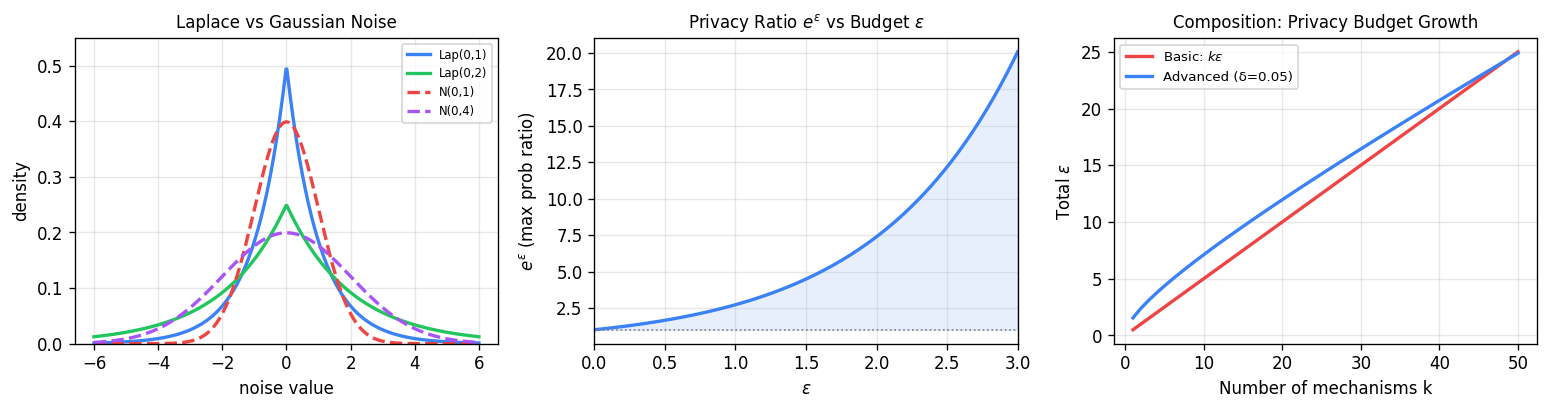
Laplace vs Gaussian noise distributions and composition budget growth

Left: Laplace noise (heavier tails, peaked center) vs Gaussian noise. Middle: the privacy ratio $e^\varepsilon$ grows exponentially with the budget $\varepsilon$ — small $\varepsilon$ keeps outputs nearly indistinguishable. Right: basic composition (linear in $k$) versus advanced composition (sublinear via $\sqrt{k}$), showing the substantial savings from advanced composition with many mechanisms.

Basic Composition

A fundamental property of differential privacy is that it composes gracefully.

Basic Composition. If $ M_1 $ is $ \varepsilon_1 $-DP and $ M_2 $ is $ \varepsilon_2 $-DP, then releasing $ (M_1(X), M_2(X)) $ is $ (\varepsilon_1 + \varepsilon_2) $-DP.

More generally, $ k $ mechanisms each satisfying $ \varepsilon $-DP together satisfy $ k\varepsilon $-DP. This allows us to decompose complex algorithms into simple $ \varepsilon_i $-DP steps and simply add up the privacy costs. The cost of composition is linear — each additional query costs $ \varepsilon $ more.

Approximate Differential Privacy

Pure $ \varepsilon $-DP is a strong guarantee, but it comes at a cost in accuracy. For example, the Gaussian mechanism does not satisfy pure DP (its tails are not bounded enough). A useful relaxation is (ε, δ)-differential privacy, also known as approximate DP.

Approximate Differential Privacy. An algorithm $ M : \mathcal{X}^n \to \mathcal{Y} $ is $(\varepsilon, \delta)$-differentially private if, for all neighbouring $ X, X' $ and all $ T \subseteq \mathcal{Y} $, \[ \Pr[M(X) \in T] \leq e^\varepsilon \cdot \Pr[M(X') \in T] + \delta. \]

The parameter $ \delta $ represents a small probability that the multiplicative guarantee fails catastrophically. Intuitively: with probability $ 1 - \delta $ the output is $ \varepsilon $-DP, and with probability $ \delta $ anything can happen. In practice, $ \delta $ should be much smaller than $ 1/n $ — otherwise the guarantee could apply to no individual in the database.

The Privacy Loss Random Variable

A useful lens for understanding both pure and approximate DP is the privacy loss random variable.

Privacy Loss. For random variables $ Y $ and $ Z $ with matching support, the privacy loss random variable $ L_{Y \| Z} $ is defined by drawing $ t \sim Y $ and outputting \[ L_{Y \| Z} = \ln \frac{\Pr[Y = t]}{\Pr[Z = t]}. \]

When applied to $ Y = M(X) $ and $ Z = M(X') $ for neighbouring $ X, X' $, this measures how much an observer can update their belief about which database was used, upon seeing the output. Pure $ \varepsilon $-DP says $ |L_{M(X) \| M(X')}| \leq \varepsilon $ with probability 1. Approximate $ (\varepsilon, \delta) $-DP is equivalent (Lemma 3.17 of Dwork-Roth) to saying $ |L_{M(X) \| M(X')}| \leq \varepsilon $ with probability at least $ 1 - \delta $.

Chapter 3: Composition and Algorithmic Mechanisms

Advanced Composition

Basic composition gives us a linear $ k\varepsilon $ privacy cost for $ k $ queries. This is often too pessimistic. The advanced composition theorem shows that with a small $ \delta $ relaxation, the effective cost grows only as $ \sqrt{k} \varepsilon $.

Advanced Composition (Dwork, Rothblum, Vadhan, 2010). For $ \varepsilon, \delta, \delta' > 0 $, let $ M = (M_1, \ldots, M_k) $ be a sequence of (potentially adaptively chosen) $(\varepsilon, \delta)$-DP algorithms. Then $ M $ is $(\tilde{\varepsilon}, \tilde{\delta})$-differentially private where \[ \tilde{\varepsilon} = \varepsilon\sqrt{2k \ln(1/\delta')} + k\varepsilon \cdot \frac{e^\varepsilon - 1}{e^\varepsilon + 1}, \qquad \tilde{\delta} = k\delta + \delta'. \]

When $ \varepsilon $ is small (the high-privacy regime), the second term is approximately $ k\varepsilon^2/2 $, which is lower order. Choosing $ \delta' = \delta $, the leading term is $ O(\varepsilon\sqrt{k \log(1/\delta)}) $ — a factor of $ \sqrt{k} $ improvement over basic composition’s $ k\varepsilon $. The proof proceeds in two steps: first, reduce from arbitrary mechanisms to simple binary-output mechanisms that capture the privacy loss structure; then analyze composition of these binary mechanisms using moment-generating function arguments.

As an instructive exercise: the Gaussian mechanism applied to $ d $-dimensional queries achieves $ \ell_2 $ error $ O(\sqrt{d} / \varepsilon n) $ directly. Using advanced composition with Laplace noise and $ k = d $ queries, one recovers the same bound under approximate DP — demonstrating that the Gaussian mechanism is not magic, but rather a natural embodiment of advanced composition.

The Exponential Mechanism

The Laplace and Gaussian mechanisms address numerical queries. For settings where we want to output an object — a price, a ranking, a classifier — the exponential mechanism of McSherry and Talwar (2007) is the right tool.

To see why Laplace noise fails here, consider a digital goods auction: a retailer wants to set a price $ p $ maximizing revenue from $ n $ buyers with valuations $ v_1, \ldots, v_n $. The revenue function is $ R(p) = p \cdot |\{i : v_i \geq p\}| $. As $ p $ crosses a valuation threshold, revenue can drop discontinuously — adding small Laplace noise to the optimal price can destroy most of the revenue. We need a mechanism that treats prices as discrete objects with quality scores, not as continuous values to perturb.

Exponential Mechanism. Given a dataset $ X \in \mathcal{X}^n $, a set of objects $ \mathcal{H} $, and a score function $ s : \mathcal{X}^n \times \mathcal{H} \to \mathbb{R} $ with sensitivity $ \Delta s = \max_{h \in \mathcal{H}} \max_{X \sim X'} |s(X, h) - s(X', h)| $, the exponential mechanism outputs $ h \in \mathcal{H} $ with probability proportional to \[ \exp\!\left(\frac{\varepsilon \cdot s(X, h)}{2\Delta s}\right). \]

Theorem. The exponential mechanism is $\varepsilon$-differentially private.

Utility Guarantee. With probability at least $ 1 - \eta $, the exponential mechanism outputs an object $ h $ with score at least \[ \max_{h^* \in \mathcal{H}} s(X, h^*) - \frac{2\Delta s}{\varepsilon}\left(\ln |\mathcal{H}| + \ln \frac{1}{\eta}\right). \]

The loss in score compared to the optimal is only logarithmic in the number of objects. For the auction problem, this means the mechanism outputs a near-revenue-optimal price while being differentially private.

Private Multiplicative Weights

We now consider the fundamental problem of answering linear queries. A linear query over data domain $ \mathcal{X} $ is a function $ q : \mathcal{X} \to [0,1] $, extended to datasets as $ q(X) = \frac{1}{n}\sum_{i=1}^n q(X_i) $. Given a collection $ Q $ of linear queries, how many data points are needed to answer all of them privately up to accuracy $ \alpha $?

The naive approach — using the Laplace mechanism and basic composition — requires $ n = O(|Q| / \alpha\varepsilon) $ samples, linear in the number of queries. The Private Multiplicative Weights (PMW) algorithm of Hardt and Rothblum achieves a dramatically better dependence.

PMW works by maintaining a synthetic distribution over $ \mathcal{X} $. It initializes this to the uniform distribution, then iteratively finds a query on which the synthetic distribution is inaccurate (using the exponential mechanism), and updates the distribution using the multiplicative weights update rule. The key insight is that the multiplicative weights framework provides a potential function argument: the number of updates is bounded by the entropy of the target distribution, which is at most $ \log |\mathcal{X}| $.

Theorem (Hardt-Rothblum, 2010). PMW answers $ |Q| $ linear queries up to error $ \alpha $ using $ n = O\!\left(\frac{\sqrt{\log |\mathcal{X}|} \cdot \log^{1/2} |Q|}{(\alpha\varepsilon)}\right) $ samples under $(\varepsilon,\delta)$-DP.

What makes this remarkable is that the dependence on $ |Q| $ is polylogarithmic, not polynomial. The sample complexity depends only on the logarithm of the domain size and the logarithm of the number of queries — a nearly exponential improvement over the naive approach for large query families.

The price is computational efficiency: the exponential mechanism over the query set, and the representation of the synthetic distribution over $ \mathcal{X} $, can be expensive. Hardt, Ligett, and McSherry later gave the MWEM algorithm, a practically efficient variant that achieves similar bounds.

The Sparse Vector Technique

Suppose queries arrive in an online stream, and we want to identify which ones exceed some threshold $ T $. We cannot answer all queries accurately — the privacy cost of answering $ k $ queries is $ O(k/\varepsilon) $. But what if most queries are below the threshold and we only care about identifying the above-threshold ones?

The Sparse Vector Technique (SVT) exploits this structure. The key insight: we only pay a privacy cost for queries that exceed the threshold, not for queries we report as below it. In the sparse setting where only $ c $ queries cross the threshold, the cost is $ O(c \log k / \varepsilon) $ — logarithmic in the total number of queries.

Above Threshold Algorithm. Given a stream of sensitivity-1 queries $ f_1, f_2, \ldots $, a threshold $ T $, and privacy parameter $ \varepsilon $:

Sample a noisy threshold: $ \hat{T} \sim T + \mathrm{Lap}(2/\varepsilon) $.
For each query $ f_t $: sample $ \nu_t \sim \mathrm{Lap}(4/\varepsilon) $. Output $\top$ if $ f_t(X) + \nu_t \geq \hat{T} $, else output $\bot$.
Halt after $ c $ outputs of $\top$.

Theorem. The above-threshold algorithm is $\varepsilon$-differentially private for any number of queries, provided it halts after at most $ c $ outputs of $\top$. Moreover, with high probability, every query reported above threshold is truly within $ O(\log(ck)/\varepsilon) $ of the threshold, and every query truly $ \Omega(\log(ck)/\varepsilon) $ above $ T $ is reported as such.

The privacy proof is notoriously subtle. The crucial point is that adding noise to the threshold once (at the start) means the threshold is a private quantity, so reporting $\bot$ reveals almost nothing about the database. Only outputting $\top$ consumes privacy budget.

SVT has many applications: identifying outliers in a data stream, implementing the exponential mechanism over an implicit set of objects, and as a subroutine in larger algorithms.

Chapter 4: Beyond Global Sensitivity and Lower Bounds

Local Sensitivity and Its Pitfalls

All mechanisms we have seen so far add noise calibrated to the global sensitivity — the worst-case sensitivity over all possible databases. But in practice, the specific database $ X $ we hold might have much lower sensitivity. Can we exploit this?

Local Sensitivity. The local sensitivity of $ f : \mathcal{X}^n \to \mathbb{R} $ at database $ X $ is \[ \Delta_{\mathrm{LS}}(X) = \max_{X' \sim X} |f(X) - f(X')|, \]

where $ X' $ ranges over neighbours of $ X $.

The naive approach — add $ \mathrm{Lap}(\Delta_{\mathrm{LS}}(X)/\varepsilon) $ — fails because the magnitude of the noise leaks information about $ X $. Consider the function that computes the distance between the two closest points in a dataset. If $ X = \{0, 0, 0\} $, the local sensitivity is 0 (any neighbour still has two points at 0), so we would output 0 deterministically. But the neighbour $ Y = \{0, 0, 10000\} $ has local sensitivity 10000, requiring large noise. An adversary seeing either a near-zero output or a noisy large output can easily distinguish between $ X $ and $ Y $ — violating differential privacy.

Propose-Test-Release

Rather than using local sensitivity directly, Propose-Test-Release (PTR) first privately checks whether the local sensitivity is bounded, and only proceeds if the test passes.

The key quantity is the “distance to high sensitivity”: how many database modifications are needed before the local sensitivity becomes large? If this distance is itself large, then we are far from a high-sensitivity database, and we can safely add small noise. PTR privately estimates this distance using the Laplace mechanism, and releases the query result only if the (noisy) distance exceeds a threshold. The privacy cost of the test is accounted for in the overall budget.

Smooth Sensitivity

The most elegant approach is smooth sensitivity, due to Nissim, Raskhodnikova, and Smith. The idea is to smooth the local sensitivity function so that it changes slowly across databases — making it safe to calibrate noise to the smoothed version.

Smooth Sensitivity. For $ \beta > 0 $, the $\beta$-smooth sensitivity of $ f $ at $ X $ is \[ S_\beta^*(X) = \max_{k \geq 0} e^{-\beta k} \cdot \max_{X' : d(X, X') \leq k} \Delta_{\mathrm{LS}}(X'), \]

where $ d(X, X') $ is the number of entries that differ.

By construction, $ S_\beta^*(X) $ is a $ \beta $-smooth upper bound on local sensitivity: for any two neighbouring databases $ X \sim Y $, we have $ S_\beta^*(X) \leq e^\beta S_\beta^*(Y) $. Adding noise of scale $ O(S_\beta^*(X) / \alpha) $ (for appropriate Cauchy or Laplace-like distributions) gives a differentially private mechanism that adds much less noise than global sensitivity whenever the local sensitivity is small.

For example, the sample median has global sensitivity 1 (in a bounded domain) but typically much lower local sensitivity. Smooth sensitivity allows median computation with noise roughly matching the local sensitivity of the actual dataset.

Stability-Based Histograms

Another technique for going beyond global sensitivity is stability-based histograms. For counting queries over a domain $ [k] $, the global sensitivity is $ 1/n $, and the Laplace histogram adds noise $ O(k/\varepsilon) $ in total. This is costly for large $ k $.

The stability approach only releases counts for bins whose value is above a threshold (making them “stable”), and adds small Laplace noise. Bins that would be reported as empty are truly empty with high probability, so releasing their count reveals little. The resulting algorithm achieves error scaling with $ \log k $ rather than $ k $ for histogram queries.

Packing Lower Bounds

We have been building upper bounds — algorithms that achieve small error with few samples. Now we ask: can we do better? Are there matching lower bounds?

The packing technique gives information-theoretic lower bounds for differential privacy. The idea is to construct a large “packing” of databases — a collection where any two databases have very different true answers to the query — and argue that no DP algorithm can simultaneously give accurate answers on all of them.

One-Way Marginals Lower Bound. For estimating all $ d $ marginals of a binary dataset under $\varepsilon$-pure DP with error $ \alpha $, any algorithm requires $ n = \Omega(d/\varepsilon\alpha) $ samples.

Histogram Lower Bound. For answering histogram queries over $ [k] $ under $\varepsilon$-pure DP with error $ \alpha $, any algorithm requires $ n = \Omega(\log k / \varepsilon\alpha) $ samples.

Both lower bounds match the upper bounds from the Laplace mechanism up to logarithmic factors. The pure DP lower bound for one-way marginals requires $ \Omega(\sqrt{d}) $ times more samples than the approximate DP upper bound — establishing that the gap between pure and approximate DP is real and inherent.

The packing proof strategy: construct $ M $ databases that are pairwise hard to distinguish under DP. By the group privacy property of DP, any single database has output distribution that is $ e^{k\varepsilon} $-close to any database obtained by changing $ k $ entries. If there are $ M $ databases in the packing, a union bound argument shows that an algorithm with error $ \alpha $ on all of them requires $ n $ to be large enough that the distributions are well-separated.

Chapter 5: Privacy in Machine Learning

What Differential Privacy Does (and Does Not) Protect

Before diving into algorithms, it is important to understand what we should and should not expect from differential privacy in machine learning. Misunderstanding this point is surprisingly common, even in published work.

Informally, differential privacy guarantees that the algorithm’s output would be similar if any single datapoint were modified. It does not prevent the algorithm from learning accurate statistics about the population. When in doubt about whether a supposed privacy violation is real, ask yourself three questions:

Would the answer truly be fundamentally different if a single datapoint were changed?
Is this just machine learning working as intended?
If so, at what point was privacy given up?

Consider training a medical diagnosis classifier on data from HIV-positive patients. If the classifier accurately predicts HIV status from blood markers, is this a privacy violation? No — the classifier is doing its job. The privacy violation happened when the individual’s data was included in the training set, not when the classifier makes accurate predictions. Differential privacy can prevent membership inference (was individual $ i $ in the training set?), but it cannot prevent accurate classification.

A useful thought experiment: if someone’s data is included in a study, and the study finds a true correlation (say, between a gene variant and a disease), that individual’s privacy is not violated just because they carry the gene variant. The privacy concern is whether one can identify that specific individual participated in the study.

Empirical Risk Minimization

We now introduce the formal framework for private machine learning. The setting is Empirical Risk Minimization (ERM): given a dataset $ D = ((x_1, y_1), \ldots, (x_n, y_n)) $ and a loss function $ \ell $, we want to find a parameter vector $ \theta \in \mathcal{C} $ (a closed convex set) minimizing

\[ L(\theta, D) = \sum_{i=1}^n \ell(\theta, x_i, y_i). \]

We assume $ \ell(\cdot, x, y) $ is convex and $ L$-Lipschitz for all $ (x, y) $, and the diameter of $ \mathcal{C} $ is bounded by $ R $. The expected excess empirical risk of an algorithm outputting $ \hat\theta $ is $ \mathbb{E}[L(\hat\theta, D) - L(\theta^*, D)] $, where $ \theta^* = \arg\min_{\theta \in \mathcal{C}} L(\theta, D) $.

There are three broad strategies for making ERM differentially private: output perturbation, objective perturbation, and gradient perturbation.

Output Perturbation

The simplest approach: run standard (non-private) ERM to get $ \theta^* $, then add noise to the output.

\[ \hat\theta = \theta^* + \mathcal{N}(0, \sigma^2 I). \]

The sensitivity of $ \theta^* $ with respect to changes in a single datapoint is the key quantity. For strongly convex loss functions (where the minimizer changes by at most $ O(L/n\lambda) $ when one datapoint changes, with $ \lambda $ the strong convexity parameter), this gives an efficient algorithm with excess risk $ O(d L^2 / \lambda \varepsilon^2 n^2) $.

Objective Perturbation

A more clever approach due to Chaudhuri and Monteleoni: add noise to the loss function before optimizing, rather than to the output.

\[ \hat\theta = \arg\min_{\theta \in \mathcal{C}} \left[ L(\theta, D) + \langle b, \theta \rangle \right], \quad b \sim \mathcal{N}(0, \sigma^2 I). \]

Because the noise is added to the objective, it perturbs the minimizer in a data-independent way. The key advantage: the sensitivity of $ \hat\theta $ to a change in one datapoint can be bounded more tightly using strong convexity. This achieves comparable excess risk to output perturbation but applies more broadly.

Gradient Perturbation

The most practically important approach is gradient perturbation, which works naturally with iterative optimization. In projected gradient descent, we repeatedly update

\[ \theta_{t+1} = \Pi_{\mathcal{C}}\!\left[\theta_t - \eta \nabla_\theta L(\theta_t, D)\right], \]

where $ \Pi_\mathcal{C} $ denotes projection onto $ \mathcal{C} $. To privatize this, add Gaussian noise to each gradient step:

\[ \theta_{t+1} = \Pi_\mathcal{C}\!\left[\theta_t - \eta \left(\nabla_\theta L(\theta_t, D) + \mathcal{N}(0, \sigma^2 I)\right)\right]. \]

The sensitivity of a single gradient is bounded by $ L $ (the Lipschitz constant of the loss). Using advanced composition over $ T $ gradient steps, the overall algorithm is $(\varepsilon, \delta)$-DP with noise scale $ \sigma = O(LT\sqrt{\log(1/\delta)} / \varepsilon n) $.

Theorem (Bassily, Smith, Thakurta, 2014). Private gradient descent achieves expected excess empirical risk \[ O\!\left(\frac{LR}{\sqrt{n}} + \frac{LR\sqrt{d\log(1/\delta)}}{\varepsilon n}\right) \]

under $(\varepsilon,\delta)$-DP, where $ d $ is the dimension of $ \theta $ and $ R $ is the diameter of $ \mathcal{C} $.

The first term is the non-private statistical error. The second term is the privacy cost — it vanishes as $ n \to \infty $, but the rate depends on $ \sqrt{d} $. For high-dimensional models, this cost can be large.

Differentially Private SGD for Neural Networks

Modern deep learning does not fit neatly into the convex ERM framework. Neural networks are non-convex, overparameterized, and typically trained with stochastic gradient descent (SGD). The DP-SGD algorithm of Abadi, Chu, Goodfellow, McMahan, Mironov, Talwar, and Zhang (2016) adapts the gradient perturbation approach to this setting.

DP-SGD has two key components beyond standard SGD:

Per-sample gradient clipping. The gradient of the loss on a single datapoint is bounded in $ \ell_2 $-norm by a clipping threshold $ C $. This controls the sensitivity of the gradient update.

Noise addition. Gaussian noise with scale $ \sigma \sim C\sqrt{T}/\varepsilon n $ is added to each gradient step (after clipping and summing over a minibatch).

The moments accountant method tracks the privacy cost of DP-SGD more tightly than standard composition — it accumulates the $ k $-th moment of the privacy loss random variable across all steps, then converts this to an $ (\varepsilon, \delta) $ guarantee. This gives tighter bounds than advanced composition, especially for many small-noise steps.

PATE: Private Aggregation of Teacher Ensembles

An elegant alternative to DP-SGD is PATE (Private Aggregation of Teacher Ensembles), due to Papernot, Abadi, Erlingsson, Goodfellow, and Talwar. Rather than adding noise to gradient steps, PATE uses a knowledge transfer approach.

The private training data is split into $ m $ disjoint subsets, and a separate “teacher” model is trained on each subset non-privately. Given an unlabeled public dataset (not sensitive), each teacher votes on the label of each public point. The Noisy Argmax (exponential mechanism) is applied to the vote counts to select a label privately. A “student” model is then trained on these noisy labels.

The key privacy guarantee: each public point’s label depends on the private data only through the vote aggregation, and the noise added ensures differential privacy. The student model, trained only on noisy labels of public data, inherits the DP guarantee. Since the student never directly accesses private data, it provides privacy-preserving predictions.

PATE has several attractive properties: it is model-agnostic (any classifier can be a teacher or student), it produces a published model with a formal DP guarantee, and empirically it achieves competitive accuracy on benchmarks like MNIST and SVHN with strong privacy parameters.

Chapter 6: Private Statistical Estimation

Binary Mean Estimation

The simplest estimation problem is computing the mean of binary data: $ X_1, \ldots, X_n \overset{\text{iid}}{\sim} \mathrm{Bernoulli}(p) $. The empirical mean $ \hat{p} = \frac{1}{n}\sum X_i $ is an excellent estimator of $ p $, with $ |\hat{p} - p| \leq O(1/\sqrt{n}) $. Privatizing via the Laplace mechanism adds error $ O(1/\varepsilon n) $, so the total error is

\[ |p - \hat{p}_\varepsilon| \leq O\!\left(\frac{1}{\sqrt{n}} + \frac{1}{\varepsilon n}\right). \]

When $ \varepsilon = O(1) $, the privacy cost becomes negligible once $ n \geq O(1/\varepsilon) $, meaning that large datasets can be analyzed essentially for free in terms of privacy. The sample complexity to achieve error $ \alpha $ is $ n = O(1/\alpha^2 + 1/\alpha\varepsilon) $.

Gaussian Mean Estimation

For Gaussian data $ X_1, \ldots, X_n \overset{\text{iid}}{\sim} \mathcal{N}(\mu, \sigma^2 I_d) $ with known covariance, estimating $ \mu $ privately is more subtle. The challenge: the sensitivity of the sample mean depends on the range of the data. If the data is unbounded, the sensitivity is infinite.

The standard approach is to clip each data point to a bounded set before computing the mean. Clipping introduces a bias, but if the true $ \mu $ is far from the clipping boundary, the bias is small. The Laplace (or Gaussian) mechanism is then applied to the clipped mean.

A more sophisticated approach is the CoinPress algorithm of Biswas, Dong, Kamath, and Ullman. CoinPress iteratively refines the estimate of $ \mu $ using a sequence of clipping radii that shrink as the algorithm homes in on the true mean. This avoids the large bias from an overly aggressive initial clip and achieves nearly optimal sample complexity:

\[ n = O\!\left(\frac{d}{\alpha^2} + \frac{\sqrt{d}}{\alpha\varepsilon}\right). \]

The first term is the statistical rate for non-private Gaussian mean estimation. The second is the privacy overhead — it scales with $ \sqrt{d}/\varepsilon $ rather than $ d/\varepsilon $, reflecting the use of the Gaussian mechanism with its $ \ell_2 $-sensitivity structure.

Heavy-Tailed Distributions

Many real-world datasets are not Gaussian — they exhibit heavy tails where occasional very large values dominate the sample mean. Heavy tails pose a challenge for private mean estimation: a single outlier can have enormous sensitivity, forcing the algorithm to add a correspondingly large amount of noise.

Kamath, Singhal, and Ullman study private mean estimation for distributions with bounded $ k $-th moments (but possibly infinite higher moments). They show that, unlike the non-private setting where the sample mean is near-optimal, private mean estimation of heavy-tailed distributions requires fundamentally different algorithms. The key insight is that outlier-robust estimators (like the trimmed mean or Huber estimator) naturally have bounded sensitivity, making them better suited for private estimation. The sample complexity under $ \varepsilon $-DP scales with the tail behavior: for distributions with bounded second moments, the overhead over the non-private rate is $ O(1/\varepsilon^2) $ samples.

Finite-sample confidence intervals are a natural goal for private inference. Karwa and Vadhan construct differentially private confidence intervals for the mean of a Gaussian distribution with finite-sample validity guarantees. Unlike asymptotic confidence intervals (which are valid only for large $ n $), their intervals are valid for any sample size, at the cost of a slightly larger interval width.

Chapter 7: Adaptive Data Analysis

The Reproducibility Crisis and Adaptivity

Modern scientific practice often involves a cycle of hypothesis formation and testing on the same dataset: a researcher analyzes data, finds a surprising result, runs further tests, refines hypotheses, and so on. This adaptive data analysis — where subsequent queries depend on earlier results — is a primary driver of the reproducibility crisis in science.

To see why adaptivity is dangerous, consider an analyst who runs 20 independent hypothesis tests on a dataset, each at significance level $ \alpha = 0.05 $. By chance, one test will appear significant even if all null hypotheses are true (false discovery rate ≈ $ 1 - 0.95^{20} \approx 64\% $). But the problem runs deeper: if the analyst selects which hypothesis to test based on earlier results, the effective number of tests is much larger than 20, and the false discovery rate can be arbitrarily high.

Differential Privacy as a Stability Guarantee

Dwork, Feldman, Hardt, Pitassi, Reingold, and Roth established a remarkable connection: differential privacy implies generalization in adaptive data analysis.

Theorem (Dwork et al., 2015). If an algorithm $ A $ is $(\varepsilon, \delta)$-DP, and is applied to a dataset $ X \sim D^n $, then for any function $ \phi $ with $ |\phi| \leq 1 $, \[ |\mathbb{E}_X[\phi(A(X))] - \mathbb{E}_{x \sim D}[\phi(x)]| \leq O\!\left(\sqrt{\frac{\log(1/\delta)}{n}} + \varepsilon\right). \]

In words: a DP algorithm that computes statistics on a sample generalizes to the underlying population, even when the statistics are computed adaptively. This is a stability guarantee: DP algorithms are not overfit to the specific sample they see.

The key mechanism: because DP limits how much any single datapoint influences the output, the algorithm’s result cannot be too tightly coupled to the specific sample. This implies generalization by a stability argument — any algorithm that depends too strongly on the sample is non-private, and conversely, any DP algorithm must generalize.

This insight opens up a principled approach to adaptive data analysis: answer queries adaptively using a DP mechanism, and the answers will generalize to fresh data. Jung, Ligett, Neel, Roth, Sharifi-Malvajerdi, and Shenfeld refined this analysis to show that the generalization guarantee of a DP algorithm applied adaptively is essentially as good as if the queries were non-adaptive — a strong robustness guarantee for empirical science.

Chapter 8: Deploying Differential Privacy

The Local Model

For most of this course, we have worked in the central model of differential privacy: a trusted curator holds all the raw data and releases DP statistics. But in many real-world settings, there is no trusted curator — users must protect their own data before sending it to anyone.

The local model of differential privacy formalizes this. Each user $ i $ with data $ X_i $ applies a locally DP mechanism before sending anything. The untrusted aggregator sees only the privatized reports $ Y_1, \ldots, Y_n $.

The local model is strictly stronger for the user: their data never leaves their device in unprotected form. But it comes at a significant statistical cost. For binary mean estimation, the central Laplace mechanism achieves error $ O(1/\varepsilon n) $. In the local model, randomized response gives error $ O(1/\varepsilon\sqrt{n}) $ — a factor of $ \sqrt{n} $ worse. For many problems, local DP requires quadratically more data than central DP to achieve the same accuracy.

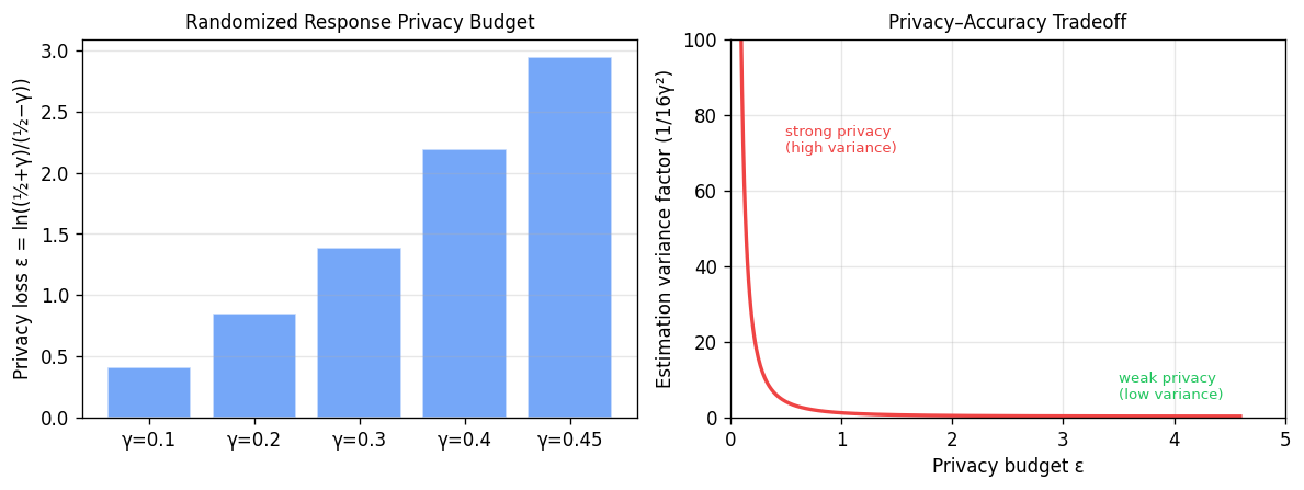
Randomized response privacy budget and accuracy-privacy tradeoff

Left: as the bias parameter $\gamma$ increases, the privacy budget $\varepsilon$ increases (weaker privacy). Right: the fundamental privacy–accuracy tradeoff — stronger privacy (small $\varepsilon$) forces larger estimation variance.

RAPPOR: Google’s Deployment

Google’s RAPPOR (Randomized Aggregatable Privacy-Preserving Ordinal Response), described by Erlingsson, Pihur, and Korolova (2014), is one of the first large-scale industrial deployments of local differential privacy. It is used in Chrome to collect statistics about browser settings, default search engines, and other configurations.

RAPPOR uses two layers of randomized response. First, each user’s categorical value is encoded as a Bloom filter — a bit string of length $ h $ where $ k $ hash functions indicate which bits to set. This “permanent randomized response” is computed once per user and retained locally, providing long-term consistency. Second, for each report, the permanent response undergoes another round of randomization (the “instantaneous randomized response”) before being sent to Google. The two-layer structure allows Google to collect statistics without linking reports from the same user across time.

The statistical analysis of RAPPOR requires careful deconvolution to recover the original distribution from the noisy reports. For a domain of size $ |\mathcal{X}| $, accurate estimation requires approximately $ n = O(|\mathcal{X}| / \varepsilon^2) $ users — the quadratic dependence on $ 1/\varepsilon $ is characteristic of local DP.

Apple’s Deployment

Apple uses local DP in iOS to collect statistics about emoji usage, health app features, and other sensitive behaviors. Their system, described in a 2017 technical report, is notable for its privacy budget management. Rather than a single DP mechanism, Apple uses a combination of count-min sketch data structures with local randomization, plus a privacy budget that resets daily. Each day’s report is independently DP, and separate mechanisms are used for different data types.

Apple’s deployment uses relatively large values of $ \varepsilon $ (reportedly $ \varepsilon = 14 $ for some mechanisms), which prompted academic discussion about the practical meaning of privacy guarantees at these parameter values. The system is designed for a specific class of high-dimensional histogram queries where central DP would be infeasible.

Microsoft and Windows 10 Telemetry

Microsoft’s collection of Windows 10 telemetry data using differential privacy, described by Ding, Kulkarni, and Yekhanin (2017), focuses on collecting time series data — how user behavior changes over time. Their dSFB (d Saturating Frequency Bit) mechanism handles the challenge that the same user contributes data across multiple days, meaning naive composition would accumulate too much privacy cost.

Their solution is to design a mechanism where each user’s contribution across all time steps has bounded total sensitivity, effectively amortizing the privacy cost. The mechanism uses a Fourier analysis approach: instead of tracking individual counts, it collects the Fourier coefficients of the time series, which have lower sensitivity for the smooth trends they care about.

The Shuffle Model

Both the central and local models have limitations: the central model requires trust in the curator, while the local model pays a large statistical price. The shuffle model offers a middle ground, as formalized in a series of papers on “amplification by shuffling.”

The key insight is that local DP is privacy-amplified when the reports from all users are randomly shuffled before being seen by the aggregator. If the aggregator cannot link a report to its source user, then even a weak local DP guarantee can produce a strong central-DP-like guarantee for the aggregated statistics.

Amplification by Shuffling (Erlingsson, Feldman, Mironov, Raghunathan, Talwar, Thakurta, 2019). If each user applies an $\varepsilon_0$-LDP mechanism, and the reports are shuffled uniformly at random, then the shuffled protocol is $(\varepsilon, \delta)$-DP (for the analyst) with $\varepsilon = O(\varepsilon_0\sqrt{\log(1/\delta)/n})$ — exponentially smaller than the local guarantee.

This exponential amplification means that users applying relatively weak local DP (say, $ \varepsilon_0 = 1 $) in a large population of $ n = 10^6 $ users can achieve central DP with $ \varepsilon \approx 0.01 $ — essentially optimal.

Prochlo, developed at Google, is a practical systems instantiation of the shuffle model. It uses a three-layer architecture: user devices apply local randomization, an “encoder” shuffles the reports in a trusted environment (using cryptographic shuffling), and the analyzer receives shuffled, locally-randomized reports. The system is designed to handle queries about which system APIs are used by which software applications — a query where the per-user sensitivity is clear and bounded.

LinkedIn’s Deployments

LinkedIn has deployed differential privacy for two applications, both described by Rogers et al. (2020).

The Audience Engagements API enables advertisers to understand how their campaigns reach different professional demographics (job title, industry, seniority). Since this data is individually sensitive, the API applies DP mechanisms to ensure that no individual member’s behavior can be inferred from the aggregate statistics. The system uses a combination of the Laplace mechanism and sensitivity bounding through query restrictions.

Labor Market Insights uses DP to track employment changes — measuring, for instance, the growth in data science roles across different sectors. This is particularly sensitive during economic disruptions. LinkedIn applies the Gaussian mechanism to histogram queries over job transitions, with privacy budgets managed to allow useful trend analysis while protecting individual career histories.

Google’s COVID-19 Mobility Reports

During the COVID-19 pandemic in 2020, Google released Community Mobility Reports showing changes in movement patterns to help public health authorities understand the effect of lockdown policies. These reports aggregate location data from Android devices to show percentage changes in visits to grocery stores, parks, transit stations, workplaces, and residential areas, compared to a pre-pandemic baseline.

Protecting privacy in this context requires careful mechanism design: the reports must be aggregated at a geographic and temporal level where individual movements cannot be identified, while remaining accurate enough to detect real changes in behavior. Google’s approach applies differential privacy with noise calibrated to the resolution of the report — finer-grained reports (smaller geographic areas, shorter time windows) get more noise.

Facebook’s URL Dataset

Facebook released a privacy-protected dataset of URL engagement statistics — which URLs were shared on Facebook and how users engaged with them. The sensitivity of this data is considerable: which URLs a user shares or clicks on can reveal political views, health concerns, and personal relationships. Facebook applied DP mechanisms to the engagement counts, and Messing et al. describe the resulting dataset and its properties in detail.

Differential Privacy in the 2020 US Census

The most consequential real-world deployment of differential privacy is the United States Census Bureau’s use of DP for the 2020 decennial census. The census collects detailed demographic information from every household in the country, and the results determine congressional apportionment, federal funding allocation, and numerous policy decisions. It is also, as we saw in Part I, deeply vulnerable to reconstruction attacks.

The TopDown Algorithm

The Census Bureau’s approach, called the TopDown Algorithm, applies differential privacy hierarchically. The geographic hierarchy of the US (nation → states → counties → census tracts → block groups → census blocks) is traversed from top to bottom:

At each geographic level, DP measurements (using the Gaussian mechanism) are made of detailed demographic counts.
These measurements are then reconciled across the hierarchy using a constrained optimization problem — the final published counts must be non-negative integers and must be consistent across geographic levels (block counts must sum to tract counts, etc.).
The reconciliation is done using a weighted least squares algorithm (the “post-processing” step, which does not consume additional privacy budget).

The total privacy budget is split across the geographic hierarchy, with more budget allocated to levels where accuracy matters most (blocks and tracts are the most important for redistricting). The 2020 census used a total privacy loss budget of $ \varepsilon = 17.14 $, distributed across four levels.

Accuracy vs. Privacy Tradeoffs at the Census

The Census Bureau’s adoption of DP generated significant debate. Demographers and redistricting experts worried that the additional noise would compromise the accuracy of small-area statistics — particularly for small racial and ethnic minority populations in small geographic units. The Census Bureau conducted extensive research on the tradeoff between privacy and accuracy, releasing several versions of the algorithm with different privacy budgets for public evaluation.

The reconstruction attacks described in Part I were a key motivating factor. Internal experiments showed that without DP, the published aggregates were sufficient to reconstruct individual microdata records for a substantial fraction of the population — a clear and present threat to the legal obligation of confidentiality under Title 13 of the US Code.

John Abowd, the Census Bureau’s Chief Scientist, who presented these results to the research community, framed the tradeoff clearly: the question is not whether to use differential privacy, but how to tune the privacy budget to balance the dual mandate of accuracy (for apportionment and fund distribution) and confidentiality (required by law). The 2020 census represents the largest real-world deployment of differential privacy to date, and its successes and limitations continue to inform the field.