CS 335: Computational Methods in Business and Finance
Christopher Batty
Estimated study time: 1 hr 2 min
Table of contents
Instructor: Christopher Batty · Term: Fall 2020
This course covers two intertwined themes: (1) the mathematical and financial theory of option pricing, leading to the celebrated Black-Scholes equation, and (2) the computational methods needed to solve such problems on a computer, including floating point arithmetic, root finding, convergence theory, lattice methods, and Monte Carlo simulation.
Option Pricing and the Two-State Tree
European Options
A European option is a financial contract that grants its holder the right — but not the obligation — to buy or sell an underlying asset at a prescribed strike price \(K\) at a fixed future time \(T\), called the expiry or exercise time.
- A call option gives the holder the right to buy the asset at \(K\).
- A put option gives the holder the right to sell the asset at \(K\).
Let \(S(t)\) denote the time-varying price of the underlying risky asset (e.g., a stock). At expiry \(t = T\), the payoff — i.e., the value of the option — is:
- Call payoff: \(\max(S(T) - K,\, 0)\)
- Put payoff: \(\max(K - S(T),\, 0)\)
For a call, if \(S(T) > K\) we exercise: buy the asset at \(K\) from the issuer and immediately sell at the market price \(S(T)\), pocketing the difference. If \(S(T) \le K\), we simply let the option expire worthless.
import numpy as np
import matplotlib.pyplot as plt

S = np.linspace(0, 150, 500)
K = 100
call_payoff = np.maximum(S - K, 0)
put_payoff  = np.maximum(K - S, 0)

fig, axes = plt.subplots(1, 2, figsize=(10, 4))
axes[0].plot(S, call_payoff, 'b', linewidth=2)
axes[0].axvline(K, color='gray', linestyle='--', alpha=0.6)
axes[0].set_title('Call Option Payoff')
axes[0].set_xlabel('S(T)')
axes[0].set_ylabel('Payoff')
axes[0].annotate('K=100', xy=(K, 0), xytext=(K+5, 5))

axes[1].plot(S, put_payoff, 'r', linewidth=2)
axes[1].axvline(K, color='gray', linestyle='--', alpha=0.6)
axes[1].set_title('Put Option Payoff')
axes[1].set_xlabel('S(T)')
axes[1].set_ylabel('Payoff')
axes[1].annotate('K=100', xy=(K, 0), xytext=(K+5, 5))

plt.tight_layout()
plt.savefig('option_payoffs.png', dpi=120, bbox_inches='tight')
plt.show()
The Central Problem: Option Pricing
The central question of the course is: What is the fair value of an option at times \(t < T\)? When an option is initially sold, what should the seller charge?
Two-state binomial tree: \(S_0=20\), \(K=21\). The hedge ratio \(\delta=0.25\) makes the portfolio risk-free, yielding the no-arbitrage price \(V_0 = \$0.633\).
A naïve approach is the expected discounted cash flow: discount the expected payoff back to today. For our two-state example with \(S(0) = 20\), \(K = 21\), \(T = 3\) months:
- Up: \(S(T) = 22\) with probability \(p = 0.1\), payoff = 1
- Down: \(S(T) = 18\) with probability \(q = 0.9\), payoff = 0
This turns out to be wrong. We will show the correct price is $0.633 using no-arbitrage arguments.
Arbitrage and the No-Arbitrage Principle
Definition. An arbitrage opportunity exists if, starting with zero initial wealth, an investor can devise a strategy with zero probability of loss and positive probability of gain.
The key insight is to assemble a hedging portfolio \(\Pi = \delta S - V\) consisting of \(\delta\) shares of the underlying stock and a short position in the option. We choose \(\delta\) so that the portfolio has the same value in both the up and down states — making it risk-free.
\[ \delta(22) - 1 = \delta(18) - 0 \implies \delta = 0.25. \]Both cases give \(\Pi = 4.5\) at \(T\). Since the portfolio is risk-free, by the No-Arbitrage Principle it must earn the risk-free rate:
No-Arbitrage Principle. A portfolio that is risk-free must earn the risk-free rate of return.
(If it earned more, you could borrow at the risk-free rate and invest in this portfolio for guaranteed profit — an arbitrage. If it earned less, you could short the portfolio and invest the proceeds at the risk-free rate, again for guaranteed profit. Either case generates arbitrageurs who quickly push the price back to equilibrium.)
\[ \Pi_\text{today} = e^{-0.12 \times 0.25} \times 4.5 \approx 4.367. \]\[ V = \delta S - \Pi = 0.25 \times 20 - 4.367 = \$0.633. \]This is the no-arbitrage value (or fair value) of the option. Notice that this is independent of the actual probabilities \(p\) and \(q\)! The real-world probabilities do not matter for option pricing under the no-arbitrage framework.
The two-state tree illustrates several deep ideas that will recur throughout the course:
- We model risky assets as following a stochastic process — random and unpredictable.
- We use hedging (combining the option and stock) to eliminate risk and thereby determine price.
Brownian Motion and Random Walks
Modeling Uncertainty with Brownian Motion
\[ dX = \alpha\, dt + \sigma\, dZ, \]where:
- \(\alpha\, dt\) is the drift term (deterministic);
- \(\sigma\) is the volatility (how much randomness there is);
- \(dZ = \phi\sqrt{dt}\) is the random term, with \(\phi \sim N(0,1)\) a standard normal random variable.
This is a stochastic differential equation (SDE). There is no single solution — only a probability density of outcomes.
Normal Distributions
\[ p(y) = \frac{1}{\sqrt{2\pi}} e^{-y^2/2}. \]\[ E[y] = \mu, \qquad \text{Var}[y] = \beta^2. \]\[ E[\phi] = 0, \qquad E[\phi^2] = 1. \]\[ E[dX] = \alpha\, dt, \qquad \text{Var}[dX] = \sigma^2\, dt. \]import numpy as np
import matplotlib.pyplot as plt
fig, axes = plt.subplots(1, 2, figsize=(12, 4))
# Left: Normal distribution
x = np.linspace(-4, 4, 400)
pdf = np.exp(-x**2/2) / np.sqrt(2*np.pi)
axes[0].plot(x, pdf, 'b', linewidth=2)
axes[0].fill_between(x, pdf, alpha=0.15, color='blue')
axes[0].set_title(r'Standard Normal $N(0,1)$')
axes[0].set_xlabel('y')
axes[0].set_ylabel('p(y)')
# Right: Brownian motion paths
np.random.seed(42)
T, N = 1.0, 1000
dt = T/N
t = np.linspace(0, T, N+1)
for _ in range(8):
W = np.cumsum(np.sqrt(dt)*np.random.randn(N))
W = np.concatenate([[0], W])
axes[1].plot(t, W, linewidth=0.8, alpha=0.7)
axes[1].set_title('Sample Brownian Motion Paths (α=0, σ=1)')
axes[1].set_xlabel('t')
axes[1].set_ylabel('X(t)')
plt.tight_layout()
plt.savefig('brownian_motion.png', dpi=120, bbox_inches='tight')
plt.show()
The Discrete Lattice (Random Walk)
To build intuition, consider a discrete random walk on a lattice. At each time step \(\Delta t\), the variable moves:
- Up by \(\Delta h\) with probability \(p\);
- Down by \(\Delta h\) with probability \(q = 1-p\).
Limiting Behavior: Connecting Lattice to Brownian Motion
\[ \Delta h = \sigma\sqrt{\Delta t}, \qquad p - q = \frac{\alpha}{\sigma}\sqrt{\Delta t}, \]\[ p = \frac{1}{2}\!\left(1 + \frac{\alpha}{\sigma}\sqrt{\Delta t}\right), \qquad q = \frac{1}{2}\!\left(1 - \frac{\alpha}{\sigma}\sqrt{\Delta t}\right), \]the lattice walk converges in distribution to \(dX = \alpha\, dt + \sigma\, dZ\). In the limit, \(X(t) - X(0) \sim N(\alpha t,\, \sigma^2 t)\).
Non-Differentiability of Brownian Paths
\[ n \cdot \Delta h = \frac{t}{\Delta t} \cdot \sigma\sqrt{\Delta t} = \frac{\sigma t}{\sqrt{\Delta t}} \to \infty. \]The “velocity” \(\Delta X / \Delta t = \pm \sigma/\sqrt{\Delta t} \to \pm\infty\). Ordinary calculus derivatives cannot be applied to such paths, which motivates the development of Ito (stochastic) calculus in the next lecture.
Ito Calculus and Ito’s Lemma
Ito Stochastic Integral
\[ X(t) - X(0) = \int_0^t a(X(s),s)\,ds + \int_0^t b(X(s),s)\,dZ(s). \]\[ \int_0^t b(X(s),s)\,dZ(s) = \lim_{\Delta t \to 0} \sum_{j=0}^{N-1} b(X(t_j), t_j)\,\Delta Z_j. \]This is the Ito convention (evaluating at the left end). An alternative, the Stratonovich convention, uses the midpoint. In finance, we use Ito because we cannot “peek into the future” — we only know current prices, not future ones.
Key Rule: \(dZ^2 \to dt\)
\[ dZ^2 = dt \quad \text{as } \Delta t \to 0. \]Equivalently, \(\left(\int_0^t b\,dZ\right)^2 = \int_0^t b^2\,ds\). This non-obvious identity is the heart of why stochastic calculus differs from ordinary calculus.
Big-O Notation
For the Taylor-series derivation to follow, we use Big-O notation:
- \(p(x) = O(x^n)\) as \(x \to 0\): there exist \(C, \delta > 0\) such that \(|p(x)| < C|x^n|\) for all \(|x| < \delta\).
Ito’s Lemma
\[ dF = F_t\,dt + F_X\,dX + \tfrac{1}{2}F_{XX}\,dX^2 + \cdots \]Substituting \(dX^2 = b^2\,dt + O(dt^{1.5})\) and collecting terms:
\[ dF = \left(aF_X + \tfrac{b^2}{2}F_{XX} + F_t\right)dt + bF_X\,dZ. \]
This is the stochastic analogue of the chain rule. The crucial extra term, \(\tfrac{b^2}{2}F_{XX}\), arises from the \(dZ^2 = dt\) rule and has no counterpart in deterministic calculus.
Geometric Brownian Motion (GBM)
\[ dS = \mu S\,dt + \sigma S\,dZ. \]\[ d(\log S) = \left(\mu - \frac{\sigma^2}{2}\right)dt + \sigma\,dZ. \]\[ \log S(T) - \log S(0) \sim N\!\left(\left(\mu - \tfrac{\sigma^2}{2}\right)T,\; \sigma^2 T\right). \]GBM Lattice
\[ S_{j+1}^{n+1} = S_j^n\, e^{+\sigma\sqrt{\Delta t}}, \qquad S_j^{n+1} = S_j^n\, e^{-\sigma\sqrt{\Delta t}}. \]Next we will see how to price options backwards through this lattice.
Lattice Pricing and Dynamic Programming
No-Arbitrage Lattice Option Pricing
\[ V_j^n = e^{-r\Delta t}\!\left(p^* V_{j+1}^{n+1} + q^* V_j^{n+1}\right), \]\[ p^* = \frac{e^{r\Delta t} - d}{u - d}, \qquad q^* = 1 - p^*, \qquad u = e^{\sigma\sqrt{\Delta t}}, \qquad d = e^{-\sigma\sqrt{\Delta t}}. \]This expression is the discounted expected value of the option at the next time step, under the artificial “risk-neutral” probabilities \(p^*, q^*\). The real-world probabilities of stock up/down moves play no role.
Algorithm: European Call Option
- Choose \(N\) steps, \(\Delta t = T/N\).
- Compute all stock prices: \(S_j^N = S_0\, e^{(2j-N)\sigma\sqrt{\Delta t}}\) at expiry.
- Set terminal option values: \(V_j^N = \max(S_j^N - K, 0)\).
- Backward sweep: for \(n = N-1, \ldots, 0\), compute: \[ V_j^n = e^{-r\Delta t}\bigl(p^* V_{j+1}^{n+1} + (1-p^*) V_j^{n+1}\bigr). \]
- Output \(V_0^0\) as the current option price.
import numpy as np
import matplotlib.pyplot as plt

def lattice_european_call(S0, K, T, r, sigma, N):
    dt = T / N
    u = np.exp(sigma * np.sqrt(dt))
    d = 1 / u
    p_star = (np.exp(r * dt) - d) / (u - d)
    discount = np.exp(-r * dt)

    # Terminal stock prices
    j = np.arange(N + 1)
    S_T = S0 * u**j * d**(N - j)
    V = np.maximum(S_T - K, 0)

    # Backward recursion
    for n in range(N - 1, -1, -1):
        V = discount * (p_star * V[1:n+2] + (1 - p_star) * V[0:n+1])
    return V[0]

# Example: S=100, K=100, T=1yr, r=5%, sigma=20%, N=200
price = lattice_european_call(100, 100, 1.0, 0.05, 0.20, 200)
print(f"European call price: ${price:.4f}")

# Convergence plot
Ns = [10, 20, 50, 100, 200, 400, 800]
prices = [lattice_european_call(100, 100, 1.0, 0.05, 0.20, N) for N in Ns]
plt.figure(figsize=(7, 4))
plt.semilogx(Ns, prices, 'b-o', markersize=5)
plt.axhline(prices[-1], color='gray', linestyle='--', alpha=0.5, label='N=800 value')
plt.xlabel('Number of time steps N')
plt.ylabel('Option price ($)')
plt.title('Lattice Convergence: European Call')
plt.legend()
plt.tight_layout()
plt.savefig('lattice_convergence.png', dpi=120, bbox_inches='tight')
plt.show()
American Options: Early Exercise
An American option can be exercised at any time in \([0,T]\). At each lattice node we now have two choices: exercise immediately (take the payoff) or continue to hold. We should do whichever maximizes value.
\[ V_j^{c,n} = e^{-r\Delta t}\!\left(p^* V_{j+1}^{n+1} + (1-p^*)V_j^{n+1}\right). \]\[ V_j^n = \max\!\left(V_j^{c,n},\; \max(S_j^n - K, 0)\right). \]This is the key modification: simply replace the European recursion with this max. No more complex algorithm is needed. For a put option, replace payoff with \(\max(K - S_j^n, 0)\).
Convergence and the Smoothed Payoff
The lattice method has first-order accuracy in time (\(O(\Delta t)\) in general. However, accuracy degrades near the kink in the option payoff at \(S = K\), because the finite-difference delta approximation is inaccurate across a non-smooth point.
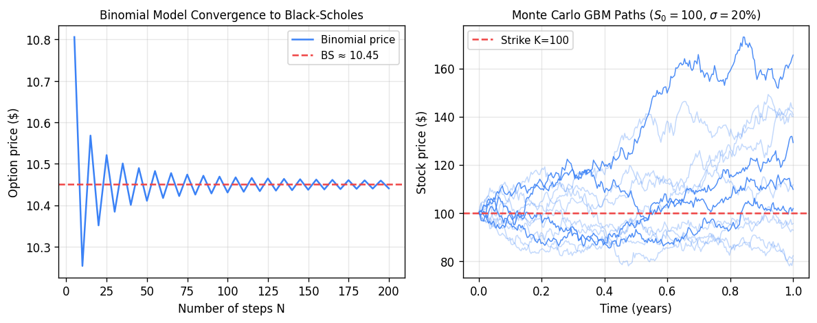
Left: binomial model price converges to the Black-Scholes price as the number of steps \(N\) increases (oscillations arise from whether the strike is above or below a node). Right: twelve GBM sample paths for \(S_0=100\), \(\sigma=20\%\), illustrating the stochastic spread of stock prices.
\[ \tilde{g}(X_j^N) = \frac{1}{2\sigma\sqrt{\Delta t}} \int_{X_j^N - \sigma\sqrt{\Delta t}}^{X_j^N + \sigma\sqrt{\Delta t}} g(x)\,dx, \]where \(g(X) = \max(e^X - K, 0)\) for a call (and \(X = \log S\). This restores second-order convergence.
Dynamic Programming: The Marriage Problem
The backward recursion underlying American option pricing is an example of dynamic programming, which exploits the principle of optimality: any sub-path of an optimal trajectory is itself optimal for the corresponding sub-problem.
To illustrate, consider the “marriage problem”: you meet \(N\) potential partners sequentially; each has a wealth drawn uniformly from \([0,1]\). You must decide at each step whether to marry the current person or move on. How do you maximize the expected wealth of your partner?
Working backwards from step \(N\):
- \(V_N = 0.5\) (expected wealth of the last person, forced to take).
- At step \(k\): marry if current person’s wealth > \(V_{k+1}\), else continue.
where \(p_k = P(W_k > V_{k+1}) = 1 - V_{k+1}\) is the probability of stopping, and \(\bar{W}_k = E[W_k \mid W_k > V_{k+1}] = \tfrac{1}{2}(1+V_{k+1})\) is the expected wealth conditional on stopping. For \(N=10\), this gives \(V_1 \approx 0.861\).
The Black-Scholes Equation and Floating Point Numbers
Deriving the Black-Scholes PDE
Under the assumptions:
- Stock follows GBM: \(dS = \mu S\,dt + \sigma S\,dZ\);
- Risk-free rate \(r\) is known;
- Short selling allowed, no transaction costs;
- Volatility \(\sigma\) is known.
Since \(\Pi\) is now risk-free, \(d\Pi = r\Pi\,dt = r(V - V_S S)\,dt\). Equating the two:
\[ V_t + \tfrac{1}{2}\sigma^2 S^2 V_{SS} + rS V_S - rV = 0. \]
The drift rate \(\mu\) of the stock does not appear — it cancels through the hedging argument. Fischer Black and Myron Scholes published this in 1973; Robert Merton shared the 1997 Nobel Prize (Black died in 1995).
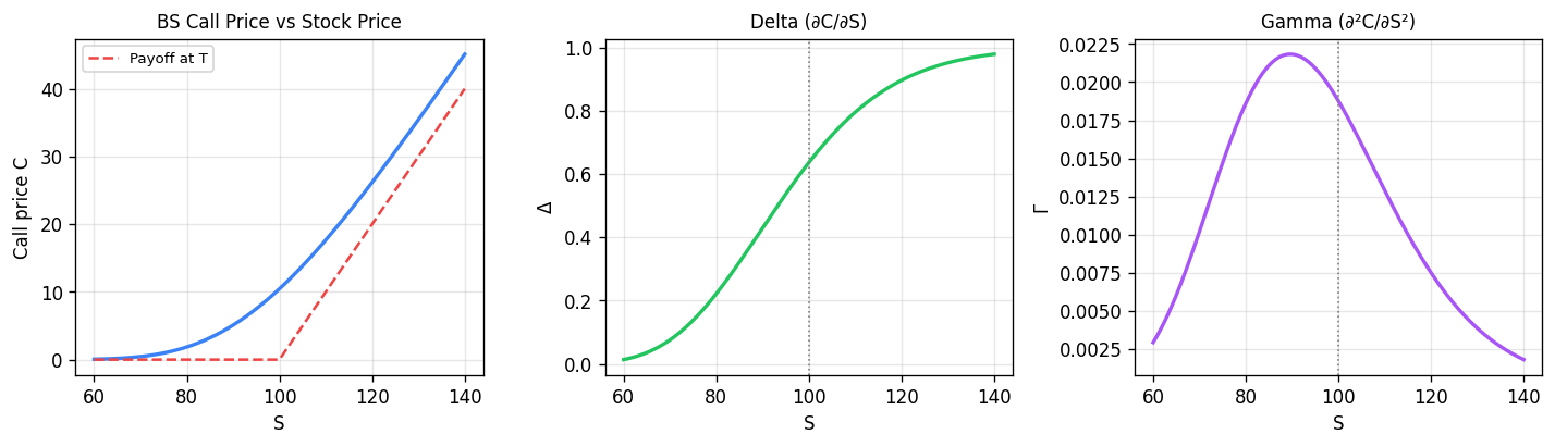
Black-Scholes call price and Greeks for \(K=100\), \(T=1\), \(r=5\%\), \(\sigma=20\%\). Delta (∂C/∂S) ranges from 0 to 1 and represents the hedge ratio; Gamma (∂²C/∂S²) peaks at-the-money and measures how rapidly the hedge must be rebalanced.
The option delta \(\delta = \partial V / \partial S\) is the number of shares to hold in the hedge. It changes continuously as \(S\) and \(t\) evolve, which is why we need continuous rebalancing (the dynamic hedge). The hedge is self-financing: given the initial proceeds from selling the option, no further cash injection is required.
Floating Point Numbers
Computers represent real numbers using floating point — a finite approximation. The real number line is infinite both in extent and density; computers can represent neither.
\[ \pm 0.d_1 d_2 \cdots d_t \times \beta^p, \quad L \le p \le U,\quad d_1 \ne 0, \]where \(\beta\) is the base, \(t\) the number of significant digits, and \([L, U]\) the exponent range.
Key properties:
- Overflow: \(p > U\) → result is \(\pm\infty\).
- Underflow: \(p < L\) → result rounds to 0.
- NaN: invalid operations like \(0/0\).
Unlike fixed-point numbers, floating point numbers are not evenly spaced — they are denser near zero and sparser far from zero.
Machine Epsilon
\[ \text{fl}(x) = x(1 + \delta), \quad |\delta| \le \varepsilon_\text{mach}. \]Formulas for \(\varepsilon_\text{mach}\):
- Rounding: \(\varepsilon_\text{mach} = \tfrac{1}{2}\beta^{1-t}\).
- Truncation/chopping: \(\varepsilon_\text{mach} = \beta^{1-t}\).
For double-precision IEEE 754 (\(\beta=2\), \(t=53\), rounding): \(\varepsilon_\text{mach} \approx 1.1 \times 10^{-16}\).
Catastrophic Cancellation
\[ E_\text{rel} \approx \frac{|x| + |y|}{|x + y|} \cdot 2\varepsilon_\text{mach}. \]- Same signs: \(|x+y| \approx |x| + |y|\), relative error \(\approx 2\varepsilon_\text{mach}\) — small.
- Opposite signs (subtraction of nearly equal numbers): \(|x+y| \ll |x| + |y|\), relative error can be catastrophically large.
This phenomenon is called catastrophic cancellation and is a major source of numerical errors.
Example. Evaluating \(e^{-5.5}\) using a Taylor series centered at \(a=0\) with \(x = -5.5\) requires summing many alternating large terms, leading to catastrophic cancellation. Using \(e^{-x} = 1/e^x\) instead avoids this.
Floating point arithmetic is not associative: \((a \oplus b) \oplus c \ne a \oplus (b \oplus c)\) in general, because each operation introduces a small rounding error and the order affects how these errors compound.
Notable disasters caused by floating point errors:
- 1982: Vancouver Stock Exchange index miscalculated by factor of 2.
- 1996: Ariane 5 rocket exploded (integer overflow: converting 64-bit float to 16-bit integer).
- 1991: US Patriot missile system failed; cumulative rounding errors caused a 0.34-second timing error.
Numerical Stability and Solving Non-Linear Equations
Conditioning and Stability
Before examining specific algorithms, two key concepts govern the quality of numerical computations:
Conditioning is a property of the mathematical problem itself. A problem is well-conditioned if small changes in input produce small changes in output. It is ill-conditioned (high condition number) if small input perturbations cause large output changes. Conditioning is independent of the numerical method.
Stability is a property of the numerical algorithm. An algorithm is stable if it does not amplify rounding errors beyond what the problem’s conditioning requires. A stable algorithm applied to a well-conditioned problem gives accurate results; even a stable algorithm applied to an ill-conditioned problem may give large errors (but that is the problem’s fault, not the algorithm’s).
The Root-Finding Problem
\[ P_\text{obs} - f(S, T, \sigma_\text{imp}, r) = 0, \]where \(f\) is the Black-Scholes formula. This is a non-linear equation in \(\sigma_\text{imp}\).
General root-finding problem: given \(f(x)\), find \(x^*\) such that \(f(x^*) = 0\).
Intermediate Value Theorem: If \(f\) is continuous on \([a,b]\) and \(f(a) \cdot f(b) < 0\) (opposite signs), then there exists \(x^* \in (a,b)\) with \(f(x^*) = 0\).
Bisection Method
Given a bracket \([a_0, b_0]\) with \(f(a_0)f(b_0) < 0\):
- Set \(x_{k+1} = (a_k + b_k)/2\).
- If \(f(a_k) \cdot f(x_{k+1}) < 0\): new bracket is \([a_k, x_{k+1}]\).
- Else: new bracket is \([x_{k+1}, b_k]\).
iterations. Bisection always works (provided \(f\) is continuous and we have a valid bracket), and always gives a guaranteed error bound.
Fixed Point Iteration
\[ x_{k+1} = g(x_k). \]Multiple choices of \(g\) are possible; not all will converge. For example, \(f(x) = x^2 - x - 2\) (root at \(x^*=2\) admits:
- \(g(x) = x^2 - 2\): \(g'(2) = 4 > 1\) — diverges.
- \(g(x) = 1 + 2/x\): \(g'(2) = -1/2\) — converges.
Newton’s Method
\[ x_{k+1} = x_k - \frac{f(x_k)}{f'(x_k)}. \]Geometrically, this follows the tangent line at \((x_k, f(x_k))\) to where it intersects the \(x\)-axis.
Secant Method
\[ f'(x_k) \approx \frac{f(x_k) - f(x_{k-1})}{x_k - x_{k-1}}, \]\[ x_{k+1} = x_k - f(x_k)\,\frac{x_k - x_{k-1}}{f(x_k) - f(x_{k-1})}. \]Requires two starting values; converges slower than Newton but faster than bisection.
import numpy as np
import matplotlib.pyplot as plt

# Visualize Newton's method for f(x) = x^2 - x - 2
def f(x):  return x**2 - x - 2
def df(x): return 2*x - 1

x = np.linspace(-1, 3.5, 400)
fig, ax = plt.subplots(figsize=(7, 5))
ax.plot(x, f(x), 'b', linewidth=2, label='f(x) = x² - x - 2')
ax.axhline(0, color='k', linewidth=0.8)
ax.axvline(2, color='gray', linestyle=':', alpha=0.6, label='root x*=2')

x0 = 3.2
colors = ['red', 'orange', 'green']
for i in range(3):
    x1 = x0 - f(x0)/df(x0)
    # Draw tangent line
    t = np.linspace(x0 - 0.8, x0 + 0.2, 50)
    ax.plot(t, f(x0) + df(x0)*(t - x0), color=colors[i],
            linewidth=1.2, linestyle='--', alpha=0.8,
            label=f'iter {i+1}: x={x1:.3f}')
    ax.plot(x0, f(x0), 'o', color=colors[i], markersize=6)
    x0 = x1

ax.set_ylim(-4, 8)
ax.set_xlabel('x')
ax.set_ylabel('f(x)')
ax.set_title("Newton's Method: 3 iterations")
ax.legend(fontsize=9)
plt.tight_layout()
plt.savefig('newtons_method.png', dpi=120, bbox_inches='tight')
plt.show()
Stopping Criteria
All iterative root-finders need a stopping rule. Common choices:
- Maximum iterations: prevent infinite loops.
- Tolerance on correction: \(|x_{k+1} - x_k| < \text{tol}\).
- Tolerance on function value: \(|f(x_k)| < \text{tol}\).
For bisection, criterion (2) gives a guaranteed error bound since \(|x_{k+1} - x_k| = (b_k - a_k)/2\) and we know \(|x_k - x^*| < b_k - a_k\). This guarantee does not hold in general for Newton or secant methods.
Convergence Theory for Root-Finding
Definition of Convergence Order
\[ \lim_{k\to\infty} \frac{e_{k+1}}{(e_k)^q} = \mu = \text{constant} \quad (< 1 \text{ if } q=1). \]- \(q = 1\): linear convergence — error halves each iteration (roughly).
- \(q = 2\): quadratic convergence — error squares each iteration (very fast).
Bisection Convergence
Bisection has linear convergence: \(e_{k+1} \le e_k/2\) on average. Each step halves the bracket, so \(|x_k - x^*| < (b_0-a_0)/2^k \to 0\). However, the actual error oscillates — on any given step, the new iterate may be closer or farther than the previous one even though the bracket has shrunk.
import numpy as np
import matplotlib.pyplot as plt

def bisection(f, a, b, tol=1e-12):
    errors = []
    x_star = 2.0  # known root
    while (b - a) > tol:
        c = (a + b) / 2
        errors.append(abs(c - x_star))
        if f(a) * f(c) < 0:
            b = c
        else:
            a = c
    return errors

def f(x): return x**2 - x - 2

errors = bisection(f, 0, 3)
plt.figure(figsize=(7, 4))
plt.semilogy(errors, 'b-o', markersize=3)
plt.xlabel('Iteration k')
plt.ylabel('|xₖ - x*| (log scale)')
plt.title('Bisection Convergence (oscillating, but overall ½ per step)')
plt.tight_layout()
plt.savefig('bisection_convergence.png', dpi=120, bbox_inches='tight')
plt.show()
Fixed Point Convergence Theorem
Theorem. Let \(g(x)\) be continuous and map \([a,b]\) into itself. If \(g\) is a contraction on \([a,b]\) — i.e., \(\exists\,\lambda \in [0,1)\) such that \(|g(x) - g(y)| \le \lambda|x-y|\) for all \(x,y \in [a,b]\) — then:
- A unique fixed point \(x^*\) exists in \([a,b]\).
- The iteration \(x_{k+1} = g(x_k)\) converges to \(x^*\) for any starting \(x_0 \in [a,b]\).
The contraction condition is essentially \(|g'(x^*)| < 1\). The convergence rate depends on \(|g'(x^*)|\):
- \(0 \le g'(x^*) < 1\): converges from one side.
- \(-1 < g'(x^*) < 0\): converges in an oscillating spiral.
- \(|g'(x^*)| > 1\): diverges.
Newton Convergence (Quadratic)
\[ e_{k+1} \approx \frac{f''(x^*)}{2f'(x^*)}\,e_k^2. \]This is quadratic convergence — once we are close, the number of correct decimal digits roughly doubles each iteration. Newton is much faster than bisection in practice, but requires:
- An initial guess reasonably close to the root.
- \(f'(x^*)\) not too small (ill-conditioned near a double root).
- Evaluating \(f'(x)\) at each step.
Secant Convergence
The secant method achieves superlinear convergence with order \(q \approx 1.618\) (the golden ratio), between linear and quadratic. It is more expensive per step than fixed point but cheaper than Newton (no derivative needed).
Summary
| Method | Order | Cost/step | Needs bracket? | Needs \(f'\)? |
|---|---|---|---|---|
| Bisection | linear (≈0.5) | 1 eval | Yes | No |
| Fixed point | linear | 1 eval | No | No |
| Secant | ≈1.618 | 1 eval | No | No |
| Newton | quadratic (2) | 2 evals | No | Yes |
Newton’s Method — Convergence Derivation
Note: Lecture 8 slides consist of handwritten OneNote pages with limited extractable text. The content below is synthesized from the course notes (§5.4) which cover the same material.
Newton Convergence Proof
\[ f(x_k) = f(x^*) + e_k f'(x^*) + \tfrac{1}{2}e_k^2 f''(x^*) + O(e_k^3) = e_k f'(x^*) + \tfrac{1}{2}e_k^2 f''(x^*) + O(e_k^3). \]\[ f'(x_k) = f'(x^*) + e_k f''(x^*) + O(e_k^2). \]\[ e_{k+1} = x_{k+1} - x^* = x_k - \frac{f(x_k)}{f'(x_k)} - x^* = e_k - \frac{e_k f'(x^*) + \tfrac{1}{2}e_k^2 f''(x^*)}{f'(x^*) + e_k f''(x^*)} + O(e_k^3). \]\[ e_{k+1} \approx \frac{f''(x^*)}{2 f'(x^*)}\, e_k^2. \]This confirms quadratic convergence. The constant \(|f''(x^*)| / |2f'(x^*)|\) governs how quickly the quadratic convergence kicks in.
Richardson Extrapolation
\[ V_\text{extrap} = \frac{2^p V_{\Delta t/2} - V_{\Delta t}}{2^p - 1} = V_\text{exact} + O(\Delta t^{p+1}). \]Richardson extrapolation is cheap (just two runs) and boosts accuracy by one order. It is widely used to improve the convergence of the lattice option pricer.
Monte Carlo Options Pricing
The Risk-Neutral World
\[ V_t + \tfrac{1}{2}\sigma^2 S^2 V_{SS} + rSV_S - rV = 0. \]The drift rate \(\mu\) does not appear. Compared to the PDE for the expected (unhedged) option value (which contains \(\mu\), the equations coincide exactly when \(\mu = r\) and the discount rate equals \(r\).
\[ V_\text{no-arb} = e^{-r(T-t)} E_Q[\text{payoff}], \]where \(E_Q\) denotes expectation in the Q-measure (risk-neutral world), where \(dS = rS\,dt + \sigma S\,dZ\).
Monte Carlo Simulation Algorithm
Instead of solving the PDE backward, we can simulate stock paths forward under the Q-measure.
\[ S_{n+1} = S_n + S_n\!\left(r\,\Delta t + \sigma\phi_n\sqrt{\Delta t}\right), \quad \phi_n \sim N(0,1). \]Algorithm:
- Simulate \(M\) independent paths from \(t=0\) to \(t=T\), each of \(N = T/\Delta t\) steps.
- For each path \(m\), compute the payoff: \(\text{payoff}_m = \max(S_N^{(m)} - K, 0)\).
- Estimate the option value: \[ V \approx e^{-rT} \cdot \frac{1}{M}\sum_{m=1}^M \text{payoff}_m. \]
import numpy as np
import matplotlib.pyplot as plt

def monte_carlo_call(S0, K, T, r, sigma, N, M, seed=42):
    np.random.seed(seed)
    dt = T / N
    S = np.full(M, S0, dtype=float)
    for _ in range(N):
        phi = np.random.randn(M)
        S = S * (1 + r*dt + sigma*phi*np.sqrt(dt))
    payoff = np.maximum(S - K, 0)
    V = np.exp(-r*T) * np.mean(payoff)
    std = np.exp(-r*T) * np.std(payoff) / np.sqrt(M)
    return V, std

V, std = monte_carlo_call(100, 100, 1.0, 0.05, 0.20, 252, 100_000)
print(f"MC estimate: ${V:.4f} ± {1.96*std:.4f} (95% CI)")

# Plot sample paths
np.random.seed(0)
S0, r, sigma, T, N = 100, 0.05, 0.20, 1.0, 252
dt = T/N
t = np.linspace(0, T, N+1)
plt.figure(figsize=(9, 4))
for _ in range(20):
    S = [S0]
    for _ in range(N):
        S.append(S[-1] * (1 + r*dt + sigma*np.random.randn()*np.sqrt(dt)))
    plt.plot(t, S, linewidth=0.7, alpha=0.6)
plt.xlabel('t (years)')
plt.ylabel('S(t)')
plt.title('Monte Carlo: 20 risk-neutral stock paths (S₀=100, r=5%, σ=20%)')
plt.tight_layout()
plt.savefig('mc_paths.png', dpi=120, bbox_inches='tight')
plt.show()
Monte Carlo Error Analysis
Two sources of error affect Monte Carlo:
\[ |E[f(S(T))] - E[f(S^{\Delta t}(T))]| \le C\,\Delta t. \]Forward Euler has weak order 1. (The weak order concerns accuracy of expectations, not individual path accuracy.)
\[ \text{Error}_\text{sampling} = O(1/\sqrt{M}). \]\[ \text{Error}_\text{MC} = O(\Delta t) + O(1/\sqrt{M}). \]\[ \text{Complexity} \propto N \times M = \frac{1}{\Delta t} \times \frac{C}{\Delta t^2} = \frac{C}{\Delta t^3} \propto \frac{1}{\text{Error}^3}. \]Reducing the error by 10× requires increasing computation by 1000×. This is MC’s main inefficiency.
MC Error Confidence Interval
\[ \hat{\mu} - \frac{x^* w}{\sqrt{M}} \le V \le \hat{\mu} + \frac{x^* w}{\sqrt{M}} \]at confidence level \(1-\alpha\), where \(x^* = 1.96\) for 95% and \(x^* = 2.58\) for 99%.
American Options via MC (Nested Simulation)
American options require comparing the early-exercise payoff against the continuation value at each step. For a single exercise time \(t_1\) (a Bermuda option):
- Simulate \(M\) paths from \(0\) to \(t_1\).
- For each path ending at \(S_A(t_1)\), spawn more simulations from \(t_1\) to \(T\) to estimate the continuation value \(e^{-r(T-t_1)}E_Q[\text{payoff}(S(T))]\).
- Take \(V(t_1) = \max(\text{early payoff},\, \text{continuation value})\).
This nested simulation (stochastic tree) requires \(M^2\) total paths and becomes exponentially expensive with more exercise dates. This is why the lattice method is preferred for American options.
Monte Carlo pros and cons:
- Pros: easy to code, naturally handles many assets and complex payoffs.
- Cons: slow convergence (\(O(1/\sqrt{M})\), difficult for American options, hard to compute “Greeks” (hedging sensitivities like delta, gamma).
Discrete Hedging
Continuous vs. Discrete Hedging
In Black-Scholes theory, a perfectly hedged portfolio requires continuous rebalancing of the delta \(\delta = \partial V / \partial S\). In practice, we can only rebalance at discrete intervals \(\Delta t_\text{hedge}\). This introduces hedging error — the portfolio value is no longer exactly zero.
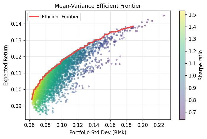
Mean-variance efficient frontier for a 5-asset portfolio. Each dot is a random portfolio; color shows Sharpe ratio (return/risk). The red curve traces the upper envelope — the set of portfolios offering maximum return for a given level of risk. This Markowitz framework underpins modern portfolio theory.
As \(\Delta t_\text{hedge} \to 0\), the hedging error vanishes; for finite intervals, there is a residual Profit & Loss (P&L).
The Delta-Hedge Simulation
Construct the portfolio: short one option, hold \(\alpha = \partial V / \partial S\) shares, with a bank account \(B\).
\[ B_0 = V_0 - \alpha_0 S_0, \qquad \Pi_0 = -V_0 + \alpha_0 S_0 + B_0 = 0. \]At each rebalancing date \(t_i\):
- Update bank account with interest: \(B_{i-1} \to B_{i-1} e^{r\Delta t}\).
- Recompute delta: \(\alpha_i = \partial V / \partial S\,(S_i, t_i)\).
- Update bank (self-financing): \[ B_i = B_{i-1} e^{r\Delta t} - (\alpha_i - \alpha_{i-1}) S_i. \] (If \(\alpha_i > \alpha_{i-1}\): buy more shares, draw from bank. If \(\alpha_i < \alpha_{i-1}\): sell shares, deposit in bank.)
If zero, the hedge was perfect.
P&L Distribution and Risk Measures
Repeating the simulation many times (under the P-measure, i.e., real-world stock paths) yields a distribution of P&L outcomes. This distribution becomes narrower as \(\Delta t_\text{hedge}\) decreases.
\[ \int_{\hat{x}}^{\infty} p(x)\,dx = \frac{y}{100}, \]so the area to the right of \(\hat{x}\) equals \(y/100\). VAR is typically reported as a positive number (the size of the potential loss), with the negative sign implied.
\[ \text{cVAR} = \frac{\int_{-\infty}^{\text{VAR}} x\,p(x)\,dx}{\int_{-\infty}^{\text{VAR}} p(x)\,dx}. \]\[ \text{cVAR}(\Pi_1 + \Pi_2) \le \text{cVAR}(\Pi_1) + \text{cVAR}(\Pi_2). \]import numpy as np
import matplotlib.pyplot as plt
from scipy.stats import norm
# Illustrate P&L distribution at two rebalancing frequencies
np.random.seed(7)
fig, axes = plt.subplots(1, 2, figsize=(11, 4))
for ax, label, scale in zip(axes, ['Δt_hedge = Δt₁', 'Δt_hedge = Δt₁/10'], [1.0, 0.32]):
pnl = np.random.normal(0, scale, 20000)
ax.hist(pnl, bins=80, density=True, color='steelblue', alpha=0.7, edgecolor='none')
# VAR at 5%
var_5 = np.percentile(pnl, 5)
ax.axvline(var_5, color='red', linewidth=1.5, label=f'95% VAR = {var_5:.2f}')
ax.set_xlabel('P&L')
ax.set_ylabel('Density')
ax.set_title(f'P&L Distribution: {label}')
ax.legend()
plt.tight_layout()
plt.savefig('pnl_distribution.png', dpi=120, bbox_inches='tight')
plt.show()
Simulating Investment Strategies
Forward Simulation and Backtesting
Forward simulation: given a stochastic model of asset prices (under the P-measure), generate many future scenarios and study the statistics of a strategy’s return (mean, stdDev, VAR, cVAR).
Backtesting: evaluate how a strategy would have performed on historical data. Backtesting is misleading because the single observed historical path is most likely one where nothing catastrophic happened — it is structurally biased toward benign outcomes and ignores tail risk. Forward simulation is more intellectually honest.
Measuring Investment Return
\[ R = \log\!\left(\frac{\Pi(T)}{\Pi(0)}\right). \]\[ E[A_\text{avg}] = E[\log X]. \]Volatility Pumping
Consider two assets:
- Asset a: doubles with prob 1/2, halves with prob 1/2 → \(E[\log X_a] = \tfrac{1}{2}\log 2 + \tfrac{1}{2}\log\tfrac{1}{2} = 0\).
- Asset b: always stays the same → \(E[\log X_b] = 0\).
Both have zero expected log return individually. Yet if we dynamically rebalance to keep 50% in each:
- Case A (prob 1/2): a doubles → total portfolio multiplier \(X = 3/2\).
- Case B (prob 1/2): a halves → total portfolio multiplier \(X = 3/4\).
By buying low and selling high at each rebalancing, the dynamic rebalancing strategy generates a positive return from two zero-return assets! This is called volatility pumping. Unfortunately, the effect is weaker in realistic GBM scenarios.
Constant Proportion Portfolio Insurance (CPPI)
CPPI (proposed by Fischer Black) provides downside protection while allowing upside participation. Define:
- \(F_i\): floor — a minimum acceptable portfolio value.
- \(M_i\): multiplier — leverage factor (often > 1).
- Cushion: \(C_i = \max(0, \Pi_i^- - F_i)\) — how far above the floor the portfolio currently sits.
Behavior:
- When \(\Pi \to F\) (portfolio approaches floor): cushion → 0, risky investment → 0, portfolio shifts entirely to risk-free assets for protection.
- When \(\Pi \gg F\): large cushion → leverage invested in risky asset for growth.
- With \(M > 1\): leverage — borrow to amplify gains.
- With \(F=0\), \(M=1/2\): reduces to the 50/50 rebalancing strategy (volatility pumping).
import numpy as np
import matplotlib.pyplot as plt

def simulate_cppi(Pi0, F0, M, r, mu, sigma, T, N, n_paths=200, seed=42):
    np.random.seed(seed)
    dt = T / N
    returns = []

    for _ in range(n_paths):
        S = 100.0
        B = Pi0 - M * max(0, Pi0 - F0)
        alpha = M * max(0, Pi0 - F0) / S

        for i in range(N):
            # Simulate stock
            phi = np.random.randn()
            S_new = S * np.exp((mu - 0.5*sigma**2)*dt + sigma*phi*np.sqrt(dt))

            # Portfolio value before rebalance
            Pi_minus = B * np.exp(r*dt) + alpha * S_new

            # New floor (growing at risk-free rate for simplicity)
            F_new = F0 * np.exp(r * (i+1)*dt)

            # Rebalance
            cushion = max(0, Pi_minus - F_new)
            alpha_new = M * cushion / S_new
            B_new = Pi_minus - alpha_new * S_new

            S, B, alpha = S_new, B_new, alpha_new

        Pi_T = B + alpha * S
        returns.append(np.log(Pi_T / Pi0))

    return np.array(returns)

# Simulate CPPI with M=4, F=80% of initial wealth
log_rets = simulate_cppi(Pi0=100, F0=80, M=4, r=0.03, mu=0.08, sigma=0.20, T=1, N=252)

fig, ax = plt.subplots(figsize=(8, 4))
ax.hist(log_rets, bins=50, density=True, color='steelblue', alpha=0.75, edgecolor='none')
var_5  = np.percentile(log_rets, 5)
cvar_5 = log_rets[log_rets <= var_5].mean()
ax.axvline(var_5,  color='red',    linewidth=1.5, linestyle='--', label=f'95% VAR = {var_5:.3f}')
ax.axvline(cvar_5, color='orange', linewidth=1.5, linestyle='-',  label=f'cVAR = {cvar_5:.3f}')
ax.set_xlabel('Log return R = log(Π(T)/Π(0))')
ax.set_ylabel('Density')
ax.set_title('CPPI Strategy: Return Distribution (M=4, Floor=80%)')
ax.legend()
plt.tight_layout()
plt.savefig('cppi_returns.png', dpi=120, bbox_inches='tight')
plt.show()
Covered Call Writing
Covered call writing is a popular income strategy: you own the underlying stock and sell a call option slightly out-of-the-money.
- At \(t=0\): own stock at \(S_0 = 100\), sell call at \(K = 105\), receive premium \(V_0\).
- Case A (\(S(T) > 105\): stock “called away” at 105; profit = \(5 + V_0\) per share — capped upside.
- Case B (\(100 - V_0 \le S(T) \le 105\): keep stock, positive return.
- Case C (\(S(T) < 100 - V_0\): stock loss partially offset by premium collected, but still a net loss.
The forward-simulated return distribution is highly left-skewed: the strategy often earns small gains (cases A and B) but has a long tail of large losses (case C, if the stock crashes). Backtesting will appear to validate this strategy because the most frequently observed historical outcome is a positive one — but the tail risk is ignored.
Summary: Key Formulas
| Concept | Formula |
|---|---|
| Brownian motion | \(dX = \alpha\,dt + \sigma\,dZ,\quad dZ = \phi\sqrt{dt},\quad \phi \sim N(0,1)\) |
| GBM (stock model) | \(dS = \mu S\,dt + \sigma S\,dZ\) |
| Ito’s lemma | \(dF = (aF_X + \tfrac{b^2}{2}F_{XX} + F_t)\,dt + bF_X\,dZ\) |
| Log of GBM | \(d(\log S) = (\mu - \tfrac{\sigma^2}{2})\,dt + \sigma\,dZ\) |
| Black-Scholes PDE | \(V_t + \tfrac{1}{2}\sigma^2 S^2 V_{SS} + rSV_S - rV = 0\) |
| Risk-neutral pricing | \(V = e^{-r(T-t)} E_Q[\text{payoff}]\) |
| Lattice risk-neutral prob | \(p^* = (e^{r\Delta t} - d)/(u-d),\; u = e^{\sigma\sqrt{\Delta t}}\) |
| Machine epsilon (round) | \(\varepsilon_\text{mach} = \tfrac{1}{2}\beta^{1-t}\) |
| Newton’s method | \(x_{k+1} = x_k - f(x_k)/f'(x_k)\) |
| MC sampling error | \(O(1/\sqrt{M})\) |
| CPPI rebalance | \(\alpha_{i+1} = M \cdot \max(0, \Pi_{i+1}^- - F_{i+1}) / S_{i+1}\) |
| Log return | \(R = \log(\Pi(T)/\Pi(0))\) |
| VAR (definition) | \(\int_{\hat{x}}^{\infty} p(x)\,dx = y/100\) |
| cVAR (definition) | Mean of P&L below VAR threshold |