CO 450/650: Combinatorial Optimization
Ricardo Fukasawa
Estimated study time: 2 hr
Table of contents
These notes are based on Felix Zhou’s course notes. Additional explanations, visualizations, and examples have been added for clarity.
Combinatorial optimization asks: given a finite set of objects each carrying a cost, find the subset satisfying some structural constraint that minimizes (or maximizes) total cost. The course develops both the algorithms and the polyhedral theory that explains why those algorithms work. The thread running through the whole course is a fruitful dialogue between combinatorial structure and linear programming duality. Beginning with spanning trees and the greedy algorithm, the course progressively reveals that the reason greedy works is the matroid axioms; that the reason weighted matching can be solved in polynomial time is a polyhedral description with an integral extreme point structure; and that the reason these polyhedral descriptions exist is total dual integrality, dual to the combinatorial structure of the problem.
Chapter 1: Spanning Trees and Greedy Algorithms
1.1 Spanning Trees
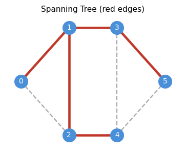
A spanning tree is the minimal connected spanning subgraph of a graph. Intuitively, it is a “backbone” that keeps all vertices reachable while discarding redundant edges. The spanning tree problem is the prototypical combinatorial optimization problem: it is simple enough to admit elegant analysis, but rich enough to generalize to matroids, matchings, and polyhedral combinatorics.
- \(V(T) = V(G)\) — it spans all vertices;
- \(T\) is connected;
- \(T\) is acyclic.
These three conditions interact deeply: any two of them, together with the count \(|E(T)| = n-1\), already imply the third. This redundancy reflects the tight combinatorial constraints that trees satisfy.
These three conditions are highly redundant — any two of them, together with \(|E(T)| = n-1\), characterize a spanning tree. The following theorem captures all the equivalent characterizations.
- (a) \(T\) is a spanning tree;
- (b) \(T\) is minimally connected;
- (c) \(T\) is maximally acyclic;
- (d) \(T\) is connected and \(|E(T)| = n-1\);
- (e) \(T\) is acyclic and \(|E(T)| = n-1\);
- (f) For all \(u,v \in V\), there is a unique \(uv\)-path in \(T\).
The equivalence of (b) and (c) is particularly elegant: a spanning tree is simultaneously the fewest edges needed for connectivity, and the most edges before a cycle appears. This min-max duality already hints at the deeper LP duality that runs throughout the course.
A useful companion result characterizes connectivity purely in terms of cuts:
Theorem 1.1.2. A graph \(G\) is connected if and only if for all \(A \subseteq V\) with \(\emptyset \neq A \neq V\), we have \(\delta(A) \neq \emptyset\).
This reframes connectivity as a property of cuts: every proper nonempty vertex set must have at least one edge leaving it.
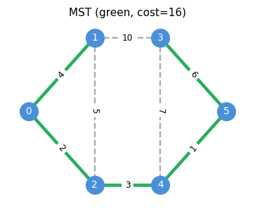
1.2 Minimum Spanning Trees
Given a connected graph \(G\) with edge costs \(c : E \to \mathbb{R}\), the minimum spanning tree (MST) problem asks for a spanning tree \(T\) minimizing (c(T) := \sum_{e \in E(T)} c_e$. Before designing an algorithm, we need to understand what makes a spanning tree optimal. The answer is a pair of local exchange conditions — the cycle and cut properties — that together completely characterize the MST.
The key optimality characterization for MSTs is the cycle property (condition b) and the cut property (condition c):
- (a) \(T\) is a MST;
- (b) Cycle property: For all \(uv \in E \setminus E(T)\), every edge \(e\) on the unique path \(T_{u,v}\) satisfies \(c_e \leq c_{uv}\);
- (c) Cut property: For all \(e \in E(T)\), if \(T_1, T_2\) are the two components of \(T - e\), then \(e\) is a minimum-cost edge in the cut \(\delta(T_1)\).
\(\neg(c) \Rightarrow \neg(b)\): If \(e \in T\) has a cheaper edge \(uv\) in the same cut, then \(e\) lies on \(T_{u,v}\) but \(c_e > c_{uv}\).
\((c) \Rightarrow (a)\): Suppose \(T\) satisfies (c) and \(T^*\) is a MST maximizing \(|E(T) \cap E(T^*)|.\) If this intersection has \(n-1\) edges, \(T = T^*\). Otherwise, pick \(uv \in E(T) \setminus E(T^*)\). The path \(T^*_{u,v}\) contains some edge \(e^* \in \delta(T_1)\). By (c), \(c_{uv} \leq c_{e^*}\), so \(T^* - e^* + uv\) is a spanning tree whose edge-intersection with \(T\) is larger — contradicting maximality. \(\square\)
The proof of \((c) \Rightarrow (a)\) uses a beautiful “exchange” argument: the cut property allows us to swap any edge of a hypothetical better spanning tree into \(T\), contradicting the maximality of the edge-intersection. This exchange paradigm will reappear in the matroid intersection theory of Chapter 3.
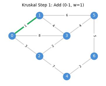
1.3 Kruskal’s Algorithm
The cycle property suggests a simple greedy algorithm: sort edges by cost and add each edge if it does not create a cycle. This is Kruskal’s algorithm, and its correctness follows directly from the optimality conditions just established.
H := (V, {})
Sort edges: c(e₁) ≤ c(e₂) ≤ ... ≤ c(eₘ)
for each edge uv in sorted order:
    if component(u) ≠ component(v):
        H.add(uv)
return H
Data structure: Union-Find for \(O(m \log m)\) sorting plus \(O(m \alpha(m,n))\) union-find operations, giving near-linear total time. Here \(\alpha\) is the inverse Ackermann function, effectively constant for all practical inputs.
The algorithm proceeds step by step, adding the cheapest safe edge at each stage:
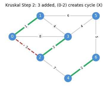
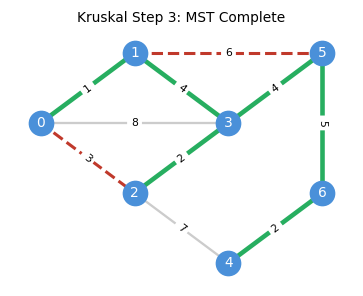
Correctness. Suppose Kruskal’s does not return an MST. Since it does return a spanning tree, there exists \(uv \in E \setminus E(H)\) and \(e \in H_{u,v}\) with \(c_{uv} < c_e\). But \(uv\) was processed before \(e\) in the sorted order and would have been added (since the endpoints were in different components at that point), a contradiction.
The correctness proof is essentially a restatement of the cycle property: Kruskal’s guarantees that every non-tree edge is at least as expensive as every tree edge on the unique tree path between its endpoints.
1.4 LP Relaxation and Complementary Slackness
Beyond the purely combinatorial analysis, there is a deeper explanation for why Kruskal’s succeeds: it is a primal-dual algorithm in disguise. The following LP perspective produces a dual certificate — a proof of optimality — constructed alongside the algorithm itself, via complementary slackness.
\[ \min \; c^T x \quad \text{s.t.} \quad x(E) = n - 1, \quad x(F) \leq n - \kappa(F) \; \forall F \subseteq E, \quad x \geq 0 \]\[ \max \sum_{F \subseteq E} (n - \kappa(F)) y_F \quad \text{s.t.} \quad \sum_{F : e \in F} y_F \leq c_e \; \forall e \in E, \quad y_F \leq 0 \; \forall F \subsetneq E. \]Proposition 1.4.1. The characteristic vector of the spanning tree produced by Kruskal’s algorithm is an optimal solution to the MST LP (PST).
The dual certificate is constructed using the edge ordering from Kruskal: set \(\bar{y}_{E_i} = c_{e_i} - c_{e_{i+1}}\) (a non-positive “step-down”) and \(\bar{y}_E = c_{e_m}\). A telescoping argument shows the dual edge constraints are tight for each \(e_i\), and the primal constraints \(x(E_i) = n - \kappa(E_i)\) confirm complementary slackness, establishing simultaneous optimality. This dual certificate is the LP proof of Kruskal’s correctness — more cumbersome than the combinatorial proof, but it generalizes to a wide class of problems where no combinatorial proof is available.
1.5 Prim’s Algorithm
While Kruskal’s algorithm processes edges globally, Prim’s algorithm grows the MST locally from a single seed vertex. An alternative to Kruskal’s is Prim’s algorithm, which grows a single tree from a root vertex by always adding the cheapest edge crossing the current tree boundary (the frontier).
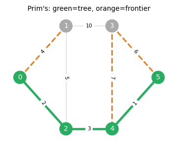
Prim’s algorithm is especially efficient with priority queues: \(O(m + n \log n)\) using Fibonacci heaps. Both Kruskal’s and Prim’s are instances of a more general greedy paradigm — one that works exactly when the underlying structure is a matroid. This observation motivates the entire next chapter.
1.6 Greedy Algorithms and the Maximum Forest
The maximum forest problem generalizes MST: given edge weights \(c : E \to \mathbb{R}\), find an acyclic subgraph \(F\) maximizing \(\sum_{e \in F} c(e)\).
This reduces to MST by negating and shifting costs. The two key propositions formalize the two directions of this reduction:
Proposition 1.5.1. The MST-reduction algorithm (connect components with cost \(-1\) edges, compute MST of \(c'_e = -c_e\), delete non-negative edges) outputs a maximum forest.
Proposition 1.5.2. Assuming the input is connected, the reduction \(c'_e := -(c_e - M) > 0\) transforms the maximum forest problem into an MST problem and returns a correct MST with respect to \(c\).
The greedy algorithm for maximum forests simply sorts edges and adds each if it does not create a cycle, stopping when costs become non-positive. The fact that this works is not obvious for general forests — it depends on the matroid structure of the forest system, which is the subject of Chapter 2.
Chapter 2: Matroids
The greedy algorithms for MST work because the set of spanning forests satisfies two simple combinatorial axioms: subsets of forests are forests (hereditary), and between two forests of different sizes, the smaller can always be augmented from the larger. These two properties are the defining axioms of a matroid — one of the central concepts of combinatorial optimization.
2.1 Definition and Motivation
Spanning forests are acyclic subgraphs — they satisfy a hereditary closure property (subsets of forests are forests) and an augmentation property (between two forests of different sizes, one can always be augmented from the other). This abstract structure is precisely a matroid. The brilliant insight of Whitney (1935) and Edmonds (1971) is that this abstraction captures exactly the class of independence systems on which the greedy algorithm is optimal.
Before defining matroids, we name the key objects in independence systems:
Definition 2.1.1 (Basis). Let \(S\) be a ground set and \(\mathcal{I} \subseteq 2^S\). A basis of \(A \subseteq S\) is an inclusionwise maximal element of \(\mathcal{I}\) contained in \(A\).
- (M1) Non-emptiness: \(\emptyset \in \mathcal{I}\);
- (M2) Hereditary: If \(F \in \mathcal{I}\) and \(F' \subseteq F\), then \(F' \in \mathcal{I}\);
- (M3) Augmentation: For all \(A \subseteq S\), every maximal independent set contained in \(A\) (basis of \(A\)) has the same cardinality.
The three axioms are minimal: removing any one of them yields structures where the greedy algorithm can fail. Axiom (M3) is the most subtle — it says that all “bases” of a set have the same size, preventing the kind of “dead end” that would trap a greedy algorithm with a suboptimal solution.
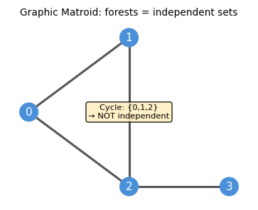
The three canonical examples are:
Example 2.1.1 (Graphic/Forest Matroid). For a graph \(G = (V, E)\), let \(\mathcal{I}\) be the set of all forests of \(G\). Then \(M = (S = E, \mathcal{I})\) is a matroid. The bases are exactly the spanning trees.
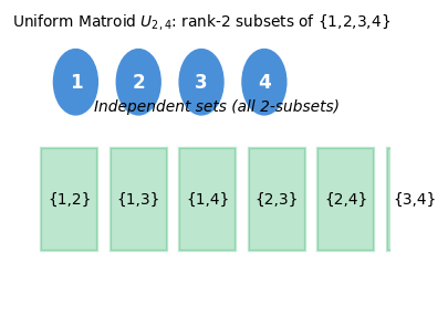
Example 2.1.2 (Uniform Matroid of Rank \(r\)). Let \(S := [n]\) and \(0 \leq r \leq n\). Let \(\mathcal{I}\) be the set of all subsets of \(S\) with at most \(r\) elements. Then \(U_r^n = (S, \mathcal{I})\) is a matroid. Every set of \(r\) elements is a basis.
Example 2.1.3 (Linear Matroid). Let \(N \in \mathbb{F}^{m \times n}\) for some field \(\mathbb{F}\) and \(S := [n]\). Let \(\mathcal{I} = \{A \subseteq S : \text{columns indexed by } A \text{ are linearly independent}\}\). Then \(M = (S, \mathcal{I})\) is a matroid.
2.2 Independence Systems and Rank
Not every independence system is a matroid. When axiom (M3) fails, we say the system is an independence system rather than a matroid. Understanding when greedy works on independence systems requires quantifying how far the system is from being a matroid — which is where the rank and lower rank come in.
If \(M = (S, \mathcal{I})\) satisfies only (M1) and (M2), it is an independence system. Elements of \(\mathcal{I}\) are independent sets; minimal dependent sets are circuits.
The rank and lower rank agree if and only if all maximal independent subsets of \(A\) have the same size — precisely the matroid condition. When they differ, the gap measures the “worst-case shortfall” in augmentation.
Proposition 2.1.4. \(M = (S, \mathcal{I})\) is a matroid if and only if \(\rho(A) = r(A)\) for all \(A \subseteq S\).
This says a matroid is exactly the independence system where all bases of every set have the same size — there are no “short” bases that trap the greedy algorithm in a suboptimal solution.
2.3 The Greedy Algorithm on Matroids
We are now ready to state the central theorem of matroid theory: the greedy algorithm is optimal if and only if the independence system is a matroid. This is a complete characterization — no partial results, no caveats.
The proof follows from the augmentation axiom: if the greedy solution fails to be optimal, one can always find an augmenting element in the optimal solution that the greedy missed, contradicting the greedy’s construction.
The counterexample construction is instructive: it uses a two-tier cost structure that forces the greedy to commit to a short basis before seeing the cheaper elements that would have led to a longer — and collectively more valuable — basis.
Even when the greedy fails, it cannot be arbitrarily bad: the rank quotient quantifies the worst-case approximation ratio.
Jenkins’ theorem is the quantitative version of the Rado–Edmonds converse: the closer the independence system is to a matroid (in the sense that all basis sizes are nearly equal), the better the greedy approximation.
2.4 Alternative Characterizations
The matroid axioms (M1)–(M3) are not the only way to characterize matroids. Several equivalent formulations — in terms of bases, circuits, and the exchange property — arise naturally in different contexts and are often more convenient to work with.
Here is one of the most remarkable facts about matroids: the same underlying combinatorial structure can be axiomatized in at least three completely different ways — through independent sets, through bases, and through circuits — and each axiomatization is “complete” in the sense that every valid matroid satisfies all three simultaneously. This is not merely a curiosity. Each axiomatization illuminates a different aspect of the structure: the independence axioms (M1)–(M3) capture the greedy-algorithm story; the basis axioms (B1)–(B2) capture the exchange story; and the circuit axioms (C1)–(C3) capture the dependency story. When you are working on a concrete problem, you choose whichever characterization is most convenient.
The circuit axioms deserve special attention. A circuit in a graphic matroid is just a cycle in the graph. The circuit elimination axiom (C3) says: if two circuits share an element \(e\), there is another circuit hiding inside their union with \(e\) removed. In the graphic matroid, this is simply the fact that composing two cycles sharing an edge produces a new cycle — a very natural property. What is remarkable is that this one property, together with minimality (C2), completely determines the matroid structure.
Theorem 2.3.1. Let \(M = (S, \mathcal{I})\) be an independence system. Then \(M\) is a matroid if and only if it satisfies: \((\text{M3}')\) for all \(X, Y \in \mathcal{I}\) with \(|X| > |Y|\), there exists \(x \in X \setminus Y\) such that \(Y \cup \{x\} \in \mathcal{I}\).
This is the more common definition in textbooks. It is equivalent to (M3): any smaller independent set can always be augmented from a larger one.
Example 2.3.2. For a graph \(G\), let \(W \subseteq V\) be a stable set. Put \(k : V \to \mathbb{Z}_+\) and consider the independence system \(S = E\), \(\mathcal{I} = \{F \subseteq E : |\delta(v) \cap F| \leq k_v, \; \forall v \in W\}\). It is easy to show that \((S, \mathcal{I})\) is a matroid through \((\text{M3}')\).
Theorem 2.3.3. Let \(M = (S, \mathcal{I})\) be a matroid. Then for all \(A \in \mathcal{I}\) and \(e \in S\), the set \(A \cup \{e\}\) contains at most one circuit.
This uniqueness of circuits in extensions is a key structural property used to define the circuit matroid operations.
Theorem 2.3.4. Let \(\mathcal{C} \subseteq 2^S\). Then \(\mathcal{C}\) is the set of circuits of a matroid if and only if:
- (C1) \(\emptyset \notin \mathcal{C}\);
- (C2) If \(C_1, C_2 \in \mathcal{C}\) and \(C_1 \subseteq C_2\), then \(C_1 = C_2\) (antichain property);
- (C3) If \(C_1 \neq C_2 \in \mathcal{C}\) and \(e \in C_1 \cap C_2\), then there exists a circuit \(C \subseteq (C_1 \cup C_2) \setminus \{e\}\) (circuit elimination).
Take a moment to appreciate what Theorem 2.3.4 is saying. You start with nothing but a collection of sets — the “forbidden” configurations — and three simple axioms about how they interact. No mention of independence, no mention of rank, no mention of greedy algorithms. Yet from these three axioms alone, the entire matroid structure springs into existence. The circuit elimination axiom (C3) is the surprising one: when two circuits share an element \(e\), there must be a “derived” circuit hiding inside their union, with \(e\) excised. In a graphic matroid this is obvious — the union of two cycles sharing an edge contains another cycle — but the axiom works in full generality, including for linear matroids, transversal matroids, and abstract matroids with no direct geometric interpretation.
This triplication of axiomatizations — independent sets, bases, circuits — is not redundant. Each tells you something different. The independent-set axioms (M1)–(M3) tell you the greedy story. The circuit axioms (C1)–(C3) tell you the obstruction story: what patterns of elements force dependence? The basis axioms (B1)–(B2) tell you the exchange story: how fluidly can you navigate between different maximal independent sets? A practitioner working on an algorithm chooses whichever language fits the problem most naturally. That a single underlying structure admits three such clean and self-contained axiomatizations is one of the deep aesthetic pleasures of matroid theory.
Theorem 2.3.5. Let \(\mathcal{B} \subseteq 2^S\). Then \(\mathcal{B}\) is the set of bases of a matroid \((S, \mathcal{I})\) if and only if:
- (B1) \(\mathcal{B} \neq \emptyset\);
- (B2) For any \(B_1, B_2 \in \mathcal{B}\) and \(x \in B_1 \setminus B_2\), there exists \(y \in B_2 \setminus B_1\) such that \((B_1 \setminus \{x\}) \cup \{y\} \in \mathcal{B}\). (Basis exchange property)
Theorem 2.3.6. \(\mathcal{B}\) is the set of bases of a matroid \((S, \mathcal{I})\) if and only if (B1) holds and also (B2’): for any \(B_1, B_2 \in \mathcal{B}\) and \(y \in B_2 \setminus B_1\), there exists \(x \in B_1 \setminus B_2\) such that \((B_1 \setminus \{x\}) \cup \{y\} \in \mathcal{B}\).
The symmetric basis exchange (B2’) is the “reverse” version of (B2): one can always swap any element of \(B_2 \setminus B_1\) into \(B_1\) and maintain a basis.
What makes Theorems 2.3.5 and 2.3.6 so useful in practice is that checking the basis exchange property is often much easier than verifying the full independence-set axioms. When you encounter a new combinatorial structure — a family of edge sets, or column sets of a matrix — and you want to know whether it is a matroid, you often proceed by showing its maximal elements satisfy (B1) and (B2). The symmetric form (B2’) is equally useful and sometimes easier to apply. Notice that (B2) and (B2’) together say that you can swap elements between any two bases in either direction: no basis is “trapped” in a region of the exchange graph unreachable from another. This global connectivity of the exchange graph is what gives matroids their algorithmic tractability.
The basis exchange property (B2) is the heart of why matroids are “the right abstraction.” In a spanning tree, adding a non-tree edge creates a unique cycle, and removing any edge of that cycle restores a spanning tree of the same size. This is exactly the basis exchange: you start with basis \(B_1\), add \(x \in B_2 \setminus B_1\) (creating a unique circuit), and recover a basis by removing some \(y \in B_1 \setminus B_2\). The fact that this works — that you can always find such a \(y\) — is the content of axiom (B2). In a matroid, no element is so “committed” to one basis that it cannot be traded away for a new one.
2.5 Polymatroids and Submodularity
The rank function of a matroid is not just any set function — it is submodular, a property with deep algorithmic and economic significance. Submodularity formalizes the principle of “diminishing returns”: the marginal value of adding an element to a set decreases as the set grows.
The motivating theorem connecting greedy and the polymatroid LP is:
Theorem 3.1.1. Let \(M = (S, \mathcal{I})\) be a matroid and \(G\) the solution returned by the greedy algorithm. Then \(x_G\) is optimal for the polymatroid LP \(\max\{c^T x : x(A) \leq r(A) \; \forall A \subseteq S,\; x \geq 0\}\).
This will be proved via complementary slackness once we develop the full greedy dual solution.
Submodularity captures diminishing returns: the “gain” from adding an element to \(A \cup B\) is no more than the sum of its gains from adding to \(A\) alone and to \(B\) alone. This is the set-function analogue of concavity.
Example 3.2.1. For a graph \(G\), let the ground set be \(V\). Then \(f(A) = |\delta(A)|\) is a submodular function.
![]()
Proposition 3.2.2. The rank function of any matroid is submodular.
The proof strategy is a careful construction of an independent set using extensions and restrictions of bases, exploiting the exchange property. It is a prototypical matroid argument.
Submodularity also connects to the LP theory of matroids through the polymatroid: the feasible region defined by the submodular rank constraints. The greedy algorithm does not just return an optimal integer solution — it returns an optimal vertex of the continuous polymatroid LP. This is a strong statement: the greedy not only works combinatorially, it works polyhedral. The dual solution constructed alongside the greedy turns out to be the complementary slack certificate that proves LP optimality simultaneously. This is the primal-dual method avant la lettre.
Proposition 3.3.1. We may assume without loss of generality that the submodular function corresponding to a polymatroid satisfies \(f(\emptyset) = 0\) and monotonicity.
Theorem 3.4.1. The primal and dual greedy solutions \(x, y\) produced by the greedy algorithm are optimal for the polymatroid LP \((P_f)\) and its dual \((D_f)\), respectively.
The proof uses complementary slackness: the greedy primal solution satisfies \(x(S_j) = f(S_j)\) for each prefix \(S_j\), matching the dual variables constructed from cost differences.
Corollary 3.4.1.1. Let \(M = (S, \mathcal{I})\), \(c \in \mathbb{R}^S\), and \(J \in \mathcal{I}\). Then \(J\) is an inclusionwise minimal, maximum weight independent set if and only if:
- (a) \(e \in J\) implies \(c_e > 0\);
- (b) \(e \notin J\), \(J \cup \{e\} \in \mathcal{I}\) implies \(c_e \leq 0\);
- (c) \(e \notin J\), \(f \in J\), and \((J \cup \{e\}) \setminus \{f\} \in \mathcal{I}\) implies \(c_e \leq c_f\).
This corollary gives a clean optimality certificate for the greedy solution: conditions (a)–(c) are exactly the complementary slackness conditions relative to the polymatroid dual.
Let us step back and admire the landscape we have just crossed. We started with a purely combinatorial algorithm — the greedy — and asked: when does it work? The answer led us to the matroid axioms, which turned out to be equivalent to three other families of axioms (circuits, bases, rank). We then discovered that the rank function of any matroid is submodular, and that the polytope defined by the submodular rank constraints — the polymatroid — is precisely the continuous relaxation of our optimization problem. The greedy algorithm simultaneously constructs the optimal primal solution (the independent set) and the optimal dual solution (the price differential variables), satisfying complementary slackness at every step. This is the primal-dual method in its purest form: building feasible primal and dual solutions together, step by step, and verifying optimality by showing all slackness conditions are met at termination. This story will repeat in different guises — for matching, for T-joins, for set cover — each time with a different combinatorial structure underpinning the same LP duality argument.
Chapter 3: Matroid Constructions and Intersection
Having established the foundations of matroid theory, we now study how matroids can be combined and modified, and culminate in the matroid intersection theorem — one of the deepest min-max results in combinatorial optimization. Matroid intersection captures bipartite matching, common bases, and many other combinatorial optimization problems within a single framework.
To appreciate how far we have come: we started by asking why Kruskal’s algorithm works on forests. The answer — the matroid axioms — turns out to be a structural property that generalizes to linear algebra (linear matroids), combinatorics (partition matroids, transversal matroids), and geometry. Now we push further: what happens when you want to optimize over the intersection of two matroid constraints simultaneously? This is the matroid intersection problem, and it admits a clean polynomial-time algorithm despite the fact that intersecting three matroids is NP-hard. The boundary between polynomial and NP-hard is sharp here, and understanding exactly where it lies is one of the gifts of this theory.
3.1 Operations on Matroids
Matroids are remarkably stable under a range of natural operations. Given a matroid \(M = (S, \mathcal{I})\), several operations yield new matroids:
- Deletion \(M \setminus B\): restrict to ground set \(S \setminus B\), same independence.
- Truncation to rank \(k\): \(\mathcal{I}' = \{A \in \mathcal{I} : |A| \leq k\}\).
- Disjoint Union: if \(M_i = (S_i, \mathcal{I}_i)\) with \(S_i\) pairwise disjoint, \(M_1 \oplus \cdots \oplus M_k\) has ground set \(\bigcup S_i\) and \(A \in \mathcal{I}\) iff \(A \cap S_i \in \mathcal{I}_i\) for all \(i\).
- Contraction \(M / B\): fix a basis \(J\) of \(B\); the contracted matroid has ground set \(S \setminus B\) and \(A \in \mathcal{I}'\) iff \(A \cup J \in \mathcal{I}\). Importantly: \(r_{M/B}(A) = r_M(A \cup B) - r_M(B)\).
- Dual \(M^* = (S, \mathcal{I}^*)\): \(A \in \mathcal{I}^*\) iff \(r(S \setminus A) = r(S)\), with rank \(r^*(A) = |A| + r_M(S \setminus A) - r_M(S)\). For the graphic matroid of a planar graph, the dual matroid is the graphic matroid of the planar dual.
These operations are not just algebraic exercises: they are the building blocks for applying matroid theory to real problems. Deletion models “what if this element is forbidden?” Contraction models “what if this element is forced to be in the solution?” Duality flips the roles of bases and cobases — in a graph, the dual matroid is the cycle matroid of the planar dual, a beautiful geometric fact. Together, they give matroids an incredibly rich algebraic structure that mirrors the structure of the problems they model.
The rank formula for contraction, \(r_{M/B}(A) = r_M(A \cup B) - r_M(B)\), is worth pausing on. It says that the rank of \(A\) in the contracted matroid is exactly the “additional rank” that \(A\) contributes beyond what \(B\) already achieves. This is the matroid analog of the dimension formula for quotient vector spaces: \(\dim(V/W) = \dim(V) - \dim(W)\). The algebraic and combinatorial structures are not just analogous — in linear matroids, the contraction literally is the quotient vector space operation. This parallel is one of the reasons linear matroids are so central to the theory: they provide geometric intuition for abstract matroid arguments.
The following formal results establish the properties of contraction and duality:
Proposition 4.1.1. Let \(M\) be the forest matroid of \(G = (V, E)\). Fix \(B \subseteq E\). Then \(M/B\) is the forest matroid of \(G/B\) (the graph obtained by contracting all edges in \(B\)).
Theorem 4.1.2. \(M/B\) is a matroid which is independent of the choice of basis \(J\) of \(B\). Moreover, \(r_{M/B}(A) = r_M(A \cup B) - r_M(B)\).
Theorem 4.1.3. The dual \(M^* = (S, \mathcal{I}^*)\) where \(\mathcal{I}^* := \{A \subseteq S : r(S \setminus A) = r(S)\}\) is a matroid with rank function \(r^*(A) = |A| + r_M(S \setminus A) - r_M(S)\).
Example 4.1.4. Consider the forest matroid \(M\) of a planar graph \(G\). Then \(A \in \mathcal{I}^*\) if and only if \(G[E \setminus A]\) has a spanning tree, i.e., \(V(E \setminus A)\) is connected. Cycles in the planar dual \(G^*\) correspond to edge cuts \(\delta(S)\) in \(G\). Thus the minimal dependent sets (circuits) of \(M^*\) are cycles, so \(M^*\) is the forest matroid of \(G^*\).
3.2 Matroid Intersection
The matroid intersection problem asks: given two matroids on the same ground set, find the largest common independent set. This generalizes bipartite matching (two partition matroids), arborescence packing (two graphic matroids), and many other problems. The min-max theorem that characterizes the optimal value is one of the deepest results in combinatorial optimization.
Pause and appreciate what the matroid intersection theorem is saying. You have two completely different types of independence constraints — say, a graph-theoretic constraint and an algebraic constraint — and you want the largest set satisfying both. This is, in general, an extraordinarily hard problem. But when both constraints happen to be matroid constraints, it becomes solvable in polynomial time. The algorithm works via augmenting paths in an auxiliary digraph — exactly paralleling the augmenting path algorithm for bipartite matching, which is itself a special case of matroid intersection (the two partition matroids on each side of the bipartition).
The min-max theorem gives the “dual certificate”: to prove that no common independent set of size \(k+1\) exists, it suffices to exhibit a partition \(A, S \setminus A\) of the ground set where \(r_1(A) + r_2(S \setminus A) = k\). This partition acts as a “cut” separating the two matroids, and its existence at the optimal value is the content of the theorem. When the two matroids are the partition matroids of a bipartite graph, this partition is exactly the minimum vertex cover of König’s theorem.
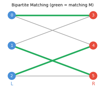
Example 5.1.1. Let \(G = (V, E)\) be bipartite with bipartition \(V_1, V_2\). For \(i = 1, 2\), let \(\mathcal{I}_i = \{A \subseteq E : |A \cap \delta(v)| \leq 1, \; \forall v \in V_i\}\). Then the maximum cardinality element of \(\mathcal{I}_1 \cap \mathcal{I}_2\) is exactly the maximum cardinality bipartite matching of \(G\).
This is a min-max theorem: the maximum common independent set has the same size as the minimum “partition certificate.” The partition \((A, S \setminus A)\) witnesses that no independent set in both matroids can exceed \(r_1(A) + r_2(S \setminus A)\) in size, since any such set can contribute at most \(r_1(A)\) elements to \(A\) (limited by \(M_1\)) and at most \(r_2(S \setminus A)\) elements to \(S \setminus A\) (limited by \(M_2\)).
Why is the matroid intersection min-max theorem so powerful? Because it simultaneously proves the existence of an efficient algorithm (the augmenting path method) and a duality theorem (the partition certificate). When you look at the optimal partition \((A, S \setminus A)\), you are looking at the “bottle-neck” of the two matroid constraints: the ground set is split in a way that the first matroid is maximally restrictive on one side and the second matroid is maximally restrictive on the other. This partition plays exactly the same role as a vertex cover in König’s theorem — it is a “certificate of difficulty” that matches the maximum achievable size. The fact that finding this partition is polynomial-time-equivalent to finding the maximum common independent set is the crux of the algorithm.
The following proposition shows how to recover König’s theorem from the matroid intersection theorem:
Proposition 5.1.3. In the bipartite matching setting, let \(M\) be a maximum matching, \(A \subseteq E\) the matroid intersection minimizer, \(B_1\) an \(M_1\)-basis of \(A\), and \(B_2\) an \(M_2\)-basis of \(E \setminus A\). Put \(U_i = B_i \cap V_i\). Then (i) \(|U_1| = r_1(A)\), (ii) \(|U_2| = r_2(E \setminus A)\), (iii) \(U_1 \cup U_2\) is a vertex cover of \(G\).
Theorem 5.1.4 (König). For a bipartite graph \(G\), \(\nu(G) = \tau(G)\).
The augmenting path algorithm for matroid intersection. The algorithm maintains a current common independent set \(J\) and looks for ways to expand it. The key idea is to build an auxiliary directed graph encoding all valid “swaps”: adding an element not in \(J\) while removing one that is, in a way that preserves independence in each matroid. An \(rs\)-directed path in this auxiliary graph is precisely an augmenting path — a sequence of swaps that extends \(J\) by one element. The correctness argument parallels Berge’s theorem for matchings: if no augmenting path exists, the current \(J\) is optimal, and the reachable vertices from \(r\) witness the optimality via the min-max formula.
Algorithm. Build an auxiliary directed graph on \(S \cup \{r, s\}\):
- Add arc \(r \to e\) if \(e \notin J\) and \(J \cup \{e\} \in \mathcal{I}_2\);
- Add arc \(e \to s\) if \(e \notin J\) and \(J \cup \{e\} \in \mathcal{I}_1\);
- For \(e \notin J\), \(f \in J\): add arc \(e \to f\) if \(J \cup \{e\} \setminus \{f\} \in \mathcal{I}_1\), and arc \(f \to e\) if \(J \cup \{e\} \setminus \{f\} \in \mathcal{I}_2\).
Lemma 5.2.1. If \(P\) is an inclusionwise minimal subset of \(S\) satisfying the augmenting path conditions \((?)\), then \(J' = J \triangle P \in \mathcal{I}_1 \cap \mathcal{I}_2\).
Lemma 5.2.2. If there is no path satisfying \((?)\), then \(J\) is a maximum cardinality element of \(\mathcal{I}_1 \cap \mathcal{I}_2\).
An \(rs\)-dipath corresponds to an augmenting path that increases \(|J \cap \mathcal{I}_1 \cap \mathcal{I}_2|\) by 1. If no such path exists, the reachable set \(U\) from \(r\) witnesses optimality via the min-max formula. The algorithm terminates in polynomial time because each augmentation strictly increases \(|J|\), and \(|J|\) is bounded by \(\min(r_1(S), r_2(S))\).
3-way intersection is NP-hard. Intersecting three matroids simultaneously is computationally intractable in general, highlighting the sharpness of the two-matroid result. This NP-hardness is not a failure of algorithmic ingenuity — it reflects a genuine combinatorial barrier: three-matroid intersection can encode Hamiltonian cycle, which is NP-complete.
The NP-hardness boundary is one of the most striking facts in this field. Two matroids: polynomial. Three matroids: NP-hard. There is no gradual degradation — the transition is abrupt. This is a strong hint that the two-matroid result is exploiting something very special about pairs of matroids that simply does not generalize to triples. Geometrically, the intersection of two matroid polytopes has a nice structure (it is the matroid intersection polytope), while three polytopes can generate arbitrarily complex integer programs.
The matroid partitioning theorem, which we state next, is a beautiful companion to matroid intersection. Rather than asking for the largest set in the intersection, it asks: how large a set can be partitioned into \(k\) independent pieces — one for each of \(k\) given matroids? The answer is again a min-max formula of the same flavor, and the proof reduces partitioning to intersection by a product-space trick. Applications include: edge coloring of graphs (partition edges into matchings), arboricity (partition edges into forests), and scheduling (partition tasks into feasible groups). In each case, the min-max formula gives an exact threshold — not an approximation — for when such a partition exists.
Definition 5.3.1 (Partitionable). Let \(M_i = (S, \mathcal{I}_i)\), \(1 \leq i \leq k\) be matroids. We say \(J \subseteq S\) is partitionable if \(J = J_1 \sqcup \cdots \sqcup J_k\) with \(J_i \in \mathcal{I}_i\) for each \(i\).
The proof reduces matroid partitioning to matroid intersection by creating \(k\) copies of \(S\) and applying the two-matroid intersection theorem.
Matroid partitioning generalizes the question “can I color the edges of a graph with \(k\) colors so that each color class is a forest?” — this is the arboricity problem, and the answer is determined exactly by the Nash-Williams formula, which is a special case of the matroid partitioning theorem. More broadly, matroid partitioning answers the question of when a combinatorial structure can be decomposed into \(k\) independent pieces, and the answer always has the clean min-max form above.
Chapter 4: Matchings
Matching theory is one of the jewels of combinatorial optimization. It begins with a deceptively simple question — which vertices can be simultaneously paired? — and unfolds into a rich theory with connections to LP duality, polyhedral combinatorics, and structural decompositions. The progression from bipartite matching (solved by augmenting paths and Hall’s theorem) to general matching (requiring Edmonds’ blossom algorithm and the Gallai-Edmonds decomposition) mirrors the progression from totally unimodular LP relaxations to the more subtle matching polytope.
4.1 Basic Definitions
To define optimality for matchings, we first need the fundamental quantities: the maximum matching number and the minimum vertex cover number.
A matching is thus a set of edges with no shared endpoints — a “perfect pairing” of some vertices. The matching number \(\nu(G)\) and vertex cover number \(\tau(G)\) are the two sides of a fundamental min-max duality.
Let \(\nu(G)\) denote the maximum matching size and \(\tau(G)\) the minimum vertex cover size. The inequality \(\nu(G) \leq \tau(G)\) is immediate (every edge in a matching needs a vertex in the cover). For bipartite graphs, equality holds — this is König’s theorem.
4.2 Augmenting Paths and Berge’s Theorem
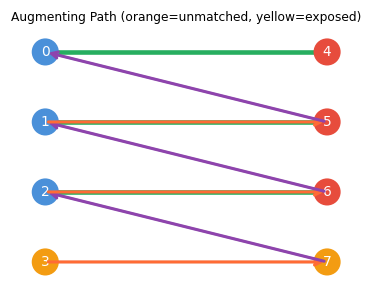
The central algorithmic idea for maximum matching is the augmenting path: a path that begins and ends at unmatched vertices, alternating between non-matching and matching edges. Flipping a matching along an augmenting path increases its size by one, and Berge’s theorem says that conversely, if no augmenting path exists, the matching is already maximum.
The alternating structure ensures that flipping the path increases the matching size by exactly one: the path has more non-matching edges than matching edges, and swapping them trades the matching edges for non-matching ones along the path.
Taking the symmetric difference \(M' = M \triangle E(P)\) along an augmenting path gives a matching of size \(|M| + 1\).
(\(\Leftarrow\)) Suppose \(M'\) is a larger matching. Consider \(G[M \triangle M']\): every vertex has degree at most 2, so it is a disjoint union of alternating paths and cycles. Since \(|M'| > |M|\), at least one path component has more \(M'\)-edges than \(M\)-edges — this is the desired augmenting path. \(\square\)
The proof leverages the symmetric difference argument: comparing two matchings via their symmetric difference reveals an augmenting path whenever one matching is larger than the other. This structural insight is the combinatorial engine of matching algorithms.
4.3 Bipartite Matching
Bipartite graphs have no odd cycles, which means blossom contractions are never needed and augmenting paths can be found by a simple BFS. For bipartite graphs, the BFS alternating-tree algorithm finds maximum matchings in polynomial time. The correctness relies on Hall’s theorem:
Hall’s theorem gives a complete certificate for the existence of a perfect matching in a bipartite graph: if no such matching exists, there is a specific “Hall-violating” set \(X \subseteq A\) with \(|N(X)| < |X|\) that witnesses the obstruction. This is a min-max theorem: the maximum matching size equals \(|A| - \max_{X \subseteq A}(|X| - |N(X)|)\).
Corollary 6.2.1.1. Let \(G\) be a bipartite graph with bipartition \(A \cup B\). There is a perfect matching if and only if \(|A| = |B|\) and \(|N(X)| \geq |X|\) for all \(X \subseteq A\).
Proposition 6.2.2. The bipartite matching algorithm correctly detects when there is no perfect matching. Specifically, at termination the alternating tree \(T\) satisfies \(N(B(T)) = A(T)\) and \(|B(T)| > |A(T)|\), witnessing a violation of Hall’s condition.
The bipartite matching algorithm grows an alternating tree from each exposed vertex. It either finds an augmenting path (improving the matching) or concludes with a frustrated tree satisfying \(N(B(T)) = A(T)\) and \(|B(T)| > |A(T)|\) — witnessing a Hall violation and hence no perfect matching.
König’s Theorem. For bipartite \(G\): \(\nu(G) = \tau(G)\). This follows from the matroid intersection theorem applied to the two partition matroids (degree constraints on each side), or alternatively from the max-flow min-cut theorem.
4.4 General Graphs and Blossoms
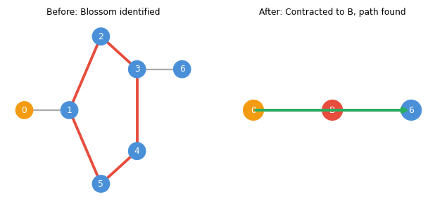
In non-bipartite graphs, the alternating tree search can become “trapped” inside an odd cycle — the blossom. The presence of a blossom does not mean no augmenting path exists; it means the path must pass through the blossom, and the algorithm must handle this correctly.
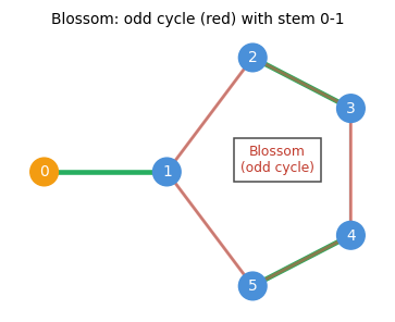
Why are odd cycles the obstruction? In a bipartite graph, every cycle is even, so when we grow an alternating tree we know exactly which side of the bipartition each vertex lies on — the two sides alternate perfectly with matching and non-matching edges. In a non-bipartite graph, an odd cycle can cause two vertices that are both “reachable by an even-length alternating path from the root” (both in the set \(B(T)\)) to be adjacent to each other. This is the blossom: two vertices of the same “parity” connected by an edge.
The naive response — just skip the edge — is wrong. The two endpoints of the blossom might be connected to unexplored parts of the graph, and the augmenting path might pass through the blossom. Edmonds’ insight is: contract the entire odd cycle to a single supernode. In the contracted graph, the supernode plays the role of a single vertex of type \(B(T)\), and the alternating tree search can continue correctly. When an augmenting path is found in the contracted graph, it can be “lifted” back to an augmenting path in the original graph — threading through the blossom in just the right way to maintain the alternating property.
When odd cycles are present, simple alternating trees can fail: two vertices in \(B(T)\) may be adjacent, creating an odd cycle (a blossom).
The blossom is the fundamental obstacle to extending bipartite matching algorithms to general graphs. Edmonds’ key insight — contracting the blossom to a supernode — resolves the difficulty cleanly.
The key insight of Edmonds’ algorithm: shrink the blossom \(C\) to a single supernode \(v_C\) and continue the algorithm in the contracted graph \(G' = G/C\). A matching in \(G'\) can be extended to a matching in \(G\) preserving the number of exposed vertices.
4.5 The Blossom Algorithm
Before presenting the algorithm, we formalize the key structural notions it uses. The algorithm maintains an alternating tree growing from an exposed vertex, and at each step one of three things happens: (a) an augmenting path is found and the matching improves; (b) the tree can be extended by a new matched edge; or (c) a blossom is detected and contracted. The algorithm terminates when the tree is “frustrated” — all neighbors of odd-distance vertices lie inside the tree — at which point the frustrated tree witnesses the non-existence of a perfect matching via Tutte’s theorem.
Definition 7.1.1 (Frustrated). An \(M\)-alternating tree \(T\) is frustrated if for all \(uv \in E\) with \(u \in B(T)\), we have \(v \in A(T)\).
Proposition 7.1.1. If \(T\) is a frustrated \(M\)-alternating tree, then \(G\) has no perfect matching.
Definition 7.1.2 (Derived Graph). The graph obtained after repeatedly shrinking blossoms is called a derived graph. For each supernode \(v\) in the derived graph, we write \(S(v)\) for the set of original vertices shrunk to form \(v\). Recursively, \(S(v) = \{v\}\) if \(v \in V(G)\), and \(S(v) = \bigcup_{w \in C} S(w)\) if \(v = v_C\) for some blossom \(C\). Note that \(|S(v)|\) is always odd.
Proposition 7.1.2. Let \(G'\) be a derived graph from \(G\) and \(M'\) a matching of \(G'\). If \(T'\) is an \(M'\)-alternating frustrated tree of \(G'\) such that all pseudonodes are in \(B(T')\), then \(G\) has no perfect matching.
Proposition 7.1.3. Let \(G'\) be a derived graph from \(G\), \(M'\) a matching of \(G'\), \(T'\) an \(M'\)-alternating tree, and \(uv \in E(G')\) with \(u, v \in B(T')\). Put \(C'\) as the unique blossom in \(T' + uv\). Then \(M'' := M' \setminus E(C')\) is a matching for \(G'' = G'/C'\) and the contracted tree \(T''\) is an \(M''\)-alternating tree in \(G''\) with the blossom vertex \(v_{C'} \in B(T'')\).
Initialize M = {}, grow alternating tree T from an exposed vertex r
while edge vw exists with v ∈ B(T), w ∉ A(T):
    if w is M-exposed:
        augment M along path in T ∪ {vw}
        restart with new exposed vertex
    elif w ∉ V(T) (w is M-covered by wx):
        extend T: add w to A(T), x to B(T)
    else (w ∈ B(T)):
        shrink blossom C = unique odd cycle in T + vw
        update G, M, T in contracted graph
if T is frustrated (all neighbors of B(T) are in A(T)):
    output "no perfect matching"
The runtime analysis hinges on the fact that each augmentation strictly increases the matching size, and each shrink reduces the number of vertices in the contracted graph.
Edmonds’ 1965 paper “Paths, Trees and Flowers” introduced the blossom algorithm — one of the first polynomial-time algorithms for a problem not obviously solvable by simple greedy or network flow methods. The key conceptual contribution was showing that odd-cycle contractions preserve the existence of augmenting paths: a fact that is geometrically obvious once stated, but historically required real creativity to discover. The paper also introduced the concept of a “good characterization” (what we now call NP ∩ co-NP), and the matching polytope theorem came a few years later as a polyhedral vindication of the blossom algorithm’s structure.
Correctness of “no perfect matching.” If the algorithm terminates with a frustrated tree \(T\), then \(N(B(T)) \subseteq A(T)\), so removing \(A(T)\) leaves \(|B(T)| > |A(T)|\) odd components. By Tutte’s theorem (below), \(G\) has no perfect matching. The frustrated tree thus serves as a Tutte obstruction — an explicit witness to the non-existence of a perfect matching.
4.6 The Tutte-Berge Formula
The Tutte-Berge formula is the matching analogue of the max-flow min-cut theorem: it expresses the maximum matching size as a minimum over all vertex sets, providing both a formula and a certificate. Tutte’s perfect matching condition is its most famous special case.
Tutte’s theorem is a min-max theorem: the maximum matching size is constrained from above by odd components, and this constraint is always tight. Every graph either has a perfect matching or has an explicit “bad” set \(A\) that creates too many odd components.
The proof of the full Tutte-Berge formula is by induction on \(|E|\), considering two cases: one endpoint of an edge is essential (covered in every maximum matching), or both are inessential. We first formalize these notions:
Definition 6.4.1 (Essential). A vertex \(u \in V\) is essential if it is \(M\)-covered in every maximum cardinality matching \(M\). Otherwise \(u\) is inessential.
Proposition 6.4.3. Let \(G = (V, E)\), \(C\) an odd cycle, and \(G' := G/C\). Let \(M'\) be a matching in \(G'\). There exists a matching \(M\) of \(G\) such that the number of \(M\)-exposed vertices of \(G\) equals the number of \(M'\)-exposed vertices of \(G'\). Consequently, \(\nu(G) \geq \nu(G') + \frac{|C|-1}{2}\).
Definition 6.4.2 (Tight). An odd cycle \(C\) is tight if \(\nu(G) = \nu(G') + \frac{|C|-1}{2}\).
Lemma 6.4.4. If \(uv \in E\) is such that both \(u\) and \(v\) are inessential, then there exists a tight odd cycle \(C\) containing \(uv\). Moreover, \(C\) is an inessential vertex of \(G' = G/C\).
The induction in the Tutte-Berge proof uses these definitions: the tight blossom contraction step preserves the formula value and enables reduction to a smaller graph.
4.7 The Gallai-Edmonds Decomposition
The Gallai-Edmonds decomposition provides a complete structural description of maximum matchings. It reveals which vertices are always covered, which are never covered, and which are sometimes covered — a partition that is both canonical (defined intrinsically) and algorithmically useful.
The Tutte-Berge formula tells us the size of the maximum matching. But knowing the optimal value is not the same as understanding the structure of optimal solutions. If you run the blossom algorithm and get a maximum matching, you might wonder: is this vertex always in the matching, or could I have left it unmatched instead? Is the exposed vertex here a necessary sacrifice, or an artifact of my choice of augmenting paths? The Gallai-Edmonds decomposition answers these questions definitively, for every graph and every maximum matching simultaneously.
Think of the decomposition as a three-actor drama. The \(D\)-vertices (the inessential ones) are the flexible players: no maximum matching is obligated to cover them, though some do. The \(A\)-vertices are the gatekeepers: they sit on the boundary between \(D\) and the rest of the graph, and every maximum matching must cover them — in fact, must match each of them to a distinct odd component of \(G[D]\). The \(C\)-vertices are the core: they form a subgraph with a perfect matching among themselves, and they have no edges to \(D\). In every maximum matching, the \(C\)-vertices are matched amongst themselves, each \(A\)-vertex is matched into \(D\), and exactly one vertex from each odd component of \(G[D]\) is left exposed. The beauty is that this structure is canonical: it does not depend on which maximum matching you found. The partition \((D, A, C)\) is a property of the graph itself.
These questions are answered by the Gallai-Edmonds decomposition, which partitions \(V\) into three sets \((D, A, C)\):
- \(D = B\) (the inessential vertices): vertices that are unmatched in at least one maximum matching. These are the “flexible” vertices.
- \(A = C\) (the “barrier” or “neighborhood of \(D\)”): vertices adjacent to \(D\) in \(V \setminus D\). Every maximum matching matches \(A\) perfectly into odd components of \(G[D]\).
- \(C = D\) (the “essential core”): vertices covered in every maximum matching, with no neighbors in \(D\). The induced subgraph \(G[C]\) has a perfect matching.
The structure theorem says that in every maximum matching, each vertex of \(A\) is matched to a distinct odd component of \(G[D]\), and within each component, the unmatched vertex of \(D\) is exposed. This gives a complete structural picture that is computationally accessible: the blossom algorithm’s frustrated trees produce the partition \((D, A, C)\) directly.
Definition 7.2.1 (Gallai-Edmonds Partition). Let \(G = (V, E)\). Put \(B\) as the set of inessential vertices. Let \(C\) be the neighbors of \(B\) in \(V \setminus B\). Set \(D = V \setminus (B \cup C)\). The triple \((B, C, D)\) is the Gallai-Edmonds partition (or decomposition) of \(G\).
yields the Gallai-Edmonds partition. In particular, \(C\) is the minimizer of the Tutte-Berge formula, \(G[B]\) has only odd components, and \(G[D]\) has only even components with a perfect matching.
The Gallai-Edmonds decomposition shows that the structure of maximum matchings is not arbitrary: there is a canonical “matching architecture” determined entirely by the graph structure.
Algorithmically, the partition \((B, C, D)\) is not just a theoretical artifact — it is directly computed by the blossom algorithm. When the blossom algorithm terminates with a collection of frustrated trees \(T_1, \ldots, T_k\), the sets \(A(T_i)\) (the odd-depth vertices in each tree) become the \(C\)-layer, the pseudonodes \(B(T_i)\) (expanded back to original vertices) become the \(D\)-layer, and all remaining vertices become the \(D\)-layer (the core). The frustrated trees are not just a certificate that no perfect matching exists — they are the proof, the algorithm’s internal data structure, and the constructor of the canonical decomposition, all at once. This is a hallmark of the best combinatorial algorithms: the algorithm computes not just the answer, but a complete structural explanation of why that answer is correct.
The blossom algorithm’s frustrated trees yield the Gallai-Edmonds partition algorithmically in polynomial time.
Proposition 7.1.5. The blossom algorithm correctly computes a maximum cardinality matching. The algorithm terminates with \(k\) frustrated trees \(T_1, \ldots, T_k\), and the final matching has exactly \(k\) exposed vertices, achieving the Tutte-Berge bound.
Chapter 5: Polyhedral Combinatorics
Up to this point, the course has used LP duality as a proof technique — to verify optimality of combinatorial algorithms. In this chapter, the relationship reverses: we study the polyhedra associated with combinatorial optimization problems and use the combinatorial structure to understand the geometry of these polyhedra. The central question is: which LPs have integer optimal solutions? The answer — total unimodularity and, more generally, total dual integrality — explains at once why network flow, bipartite matching, and T-join problems are polynomially solvable.
5.1 Weighted Matching and LP Formulations
The minimum weight perfect matching problem asks: given \(G = (V,E)\) and costs \(c : E \to \mathbb{R}\), find a perfect matching \(M\) minimizing (c(M)$. To solve this via LP, we write a relaxation and study when the relaxation is automatically integral.
\[ \min \sum_{e \in E} c_e x_e \quad \text{s.t.} \quad x(\delta(v)) = 1 \; \forall v \in V, \quad x \geq 0. \]\[ x(\delta(S)) \geq 1 \quad \forall S \subseteq V, \; |S| \text{ odd}, \; |S| \geq 3. \]These constraints are motivated by the Tutte-Berge formula: each odd set must send at least one matching edge across its boundary, so the constraint is a necessary condition for integrality.
Edmonds’ matching polytope theorem is one of the crowning achievements of polyhedral combinatorics: it gives an explicit, finite description of the convex hull of all matchings, despite the exponential number of integer points. The odd-set constraints are necessary and, together with the degree constraints, sufficient to achieve integrality.
The matching polytope theorem has a profound algorithmic consequence: since the optimal LP solution is automatically integral (it is a vertex of the matching polytope, which has integer vertices), we can solve the minimum weight perfect matching problem by solving the LP. But of course, the LP has exponentially many odd-set constraints — we cannot write them all down explicitly. The fix is the cutting plane approach: start with the LP without odd-set constraints, solve it, and if the LP solution is fractional, find a violated odd-set constraint and add it. The key question is whether we can efficiently find a violated constraint. Remarkably, this is a polynomial-time separation problem — it reduces to checking whether a minimum odd-set cut is less than 1, which can be done using the Padberg-Rao algorithm. The resulting cutting plane algorithm solves the minimum weight perfect matching problem in polynomial time, giving a polyhedral proof of what the blossom algorithm accomplishes combinatorially.
For bipartite graphs, the simpler LP (without odd-set constraints) is already integral by Birkhoff’s theorem:
Theorem 8.1.1 (Birkhoff). Let \(G\) be bipartite and \(c \in \mathbb{R}^E\). Then \(G\) has a perfect matching if and only if the primal LP is feasible. Moreover, if the primal LP is feasible, then for all minimum cost perfect matchings \(M^*\), \(\mathrm{OPT} = c(M^*)\).
The proof constructs dual variables (vertex potentials) and iteratively updates them via a frustrated-tree procedure until complementary slackness is achieved — the classical Hungarian algorithm for weighted bipartite matching. The dual variables are the vertex “prices” in the LP dual, and complementary slackness says that each matched edge is “tight” in the dual.
For general graphs, blossom shrinking must preserve dual feasibility. The following proposition formalizes the correctness of blossom contraction in the weighted setting:
Proposition 8.1.2. Let \(\bar{y}\) be feasible in the dual with \(\bar{y}_S = 0\) for all odd sets \(S \in \theta\). Let \(G', c'\) be derived from \(G, c\) by shrinking a blossom \(C\) with \(E(C) \subseteq E^=\). Let \(M'\) be a perfect matching of \(G'\) and \(y'\) feasible for the derived dual, with \(M', y'\) satisfying complementary slackness and \(y'_{v_C} \geq 0\). Extend \(M'\) to a perfect matching \(\hat{M}\) of \(G\) and define \(\hat{y}\) from \(\bar{y}\) and \(y'\). Then \(\hat{y}\) is feasible for the original dual and \(\hat{M}, \hat{y}\) satisfy the complementary slackness conditions.
Proposition 8.2.1. Let \(\bar{M}\) be a maximum weight perfect matching in \(\bar{G}\) (the doubled graph). Then \(M := \bar{M} \cap E(G)\) is a maximum weight matching in \(G\).
5.2 Vertex Covers and LP Relaxation
Vertex covers are the LP dual counterpart to matchings. The integrality (or non-integrality) of the vertex cover LP relaxation encodes the same structure that distinguishes bipartite from general graphs.
A vertex cover must “cover” every edge — the LP relaxation assigns a fractional value in \([0,1]\) to each vertex, and requires that each edge has total vertex weight at least 1. The question is when this relaxation is integral.
\[ \min \sum_v x_v \quad \text{s.t.} \quad x_u + x_v \geq 1 \; \forall uv \in E, \quad 0 \leq x_v \leq 1. \]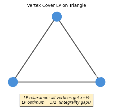
On the triangle \(K_3\), the LP optimum is \(3/2\) (set each vertex to \(1/2\)) while the integer optimum is \(2\). This integrality gap of \(4/3\) shows the LP is not always tight for general graphs. However, for bipartite graphs the LP is always integral (follows from König’s theorem via LP duality). The gap on \(K_3\) is not an artifact of a bad LP formulation — it reflects a genuine combinatorial difference between bipartite and non-bipartite graphs.
5.3 Totally Unimodular Matrices
The integrality of bipartite matching and network flow LPs has a common explanation: their constraint matrices are totally unimodular. Total unimodularity is the algebraic property that implies LP integrality for any right-hand side.
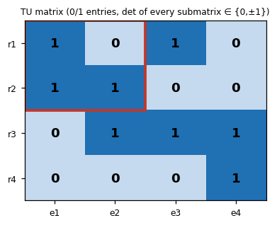
Many important combinatorial LPs are integral because their constraint matrices are totally unimodular (TU): every square submatrix has determinant in \(\{0, +1, -1\}\).
The proof follows from Cramer’s rule: the vertices of the LP feasible polyhedron are solutions to square subsystems of \(Ax = b\), and if all determinants are in \(\{0, \pm 1\}\), these solutions are integers. Total unimodularity is a gift: once a constraint matrix is known to be TU, LP relaxations are “automatically integral” for any integer right-hand side.
Examples of TU matrices:
- The incidence matrix of a bipartite graph (rows = vertices, columns = edges, each column has exactly two 1s, one in each side) is TU. This immediately implies the bipartite matching LP is integral.
- Network flow constraint matrices are TU.
- Interval matrices (rows = intervals, columns = points) are TU.
The TU property is the polyhedral explanation for why network flow, bipartite matching, and scheduling problems have polynomial-time exact algorithms via LP. It unifies a large family of tractable problems under one structural property.
There is a deep parallel here with the matroid story. In Chapter 2, we asked: for which independence systems does the greedy algorithm work? The answer was: exactly the matroids. Now we ask: for which LPs is the optimal solution always integral? The answer is: exactly the LPs with TU constraint matrices (plus integer right-hand sides). Both answers are “clean” characterization theorems — they identify exactly the right class of structures. And the connection is not coincidental: the constraint matrix of the graphic matroid (the cycle-versus-edge incidence matrix of a graph) is TU for bipartite graphs, which is precisely why bipartite matching is “easier” than general matching. Non-bipartite graphs introduce odd cycles, which destroy TU, which forces us to add odd-set constraints to the matching LP, which is why Edmonds’ matching polytope theorem requires more work than Birkhoff’s bipartite theorem.
5.4 Cutting Planes and Integer Programming
When the constraint matrix is not TU — as in general matching or set cover — the LP relaxation is not automatically integral. The solution is to strengthen the LP by adding cutting planes: valid inequalities that eliminate the fractional optimum without removing any integer feasible point. This idea, combined with branching, underlies modern integer programming solvers.
When the LP relaxation of an IP is not integral, one adds cutting planes — valid inequalities that cut off the fractional LP optimum without removing any integer feasible point.
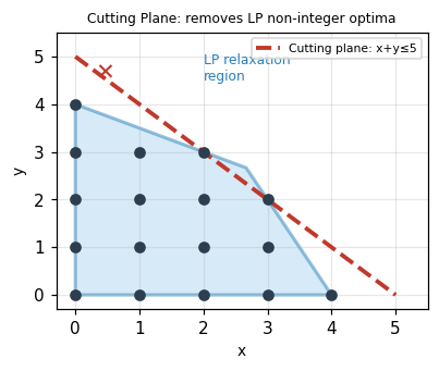
The canonical example: maximize \(x + y\) subject to \(2x + y \leq 8\), \(x + 2y \leq 8\), \(x,y \geq 0\) integer. The LP optimum is \((8/3, 8/3)\) with value \(16/3 \approx 5.33\), but the integer optimum is \(5\) at \((3,2)\) or \((2,3)\). Adding the cut \(x + y \leq 5\) (derived from rounding down the LP value) eliminates the fractional solution.
Solve LP relaxation; let x* be the optimal solution.
while x* is not integer:
    Find a valid inequality (cut) violated by x* but not by any integer feasible point.
    Add the cut to the LP and re-solve.
The Gomory cut is a systematic way to generate cuts from the LP simplex tableau. The branch-and-cut framework combines cutting planes with branching for modern integer programming solvers.
Chapter 6: T-Joins, Flows, and Cuts
The final chapter unifies the matching, flow, and polyhedral perspectives through the theory of T-joins — a generalization of matchings that captures degree-parity conditions. T-joins connect to minimum cuts via a beautiful min-max theorem, and to matchings via a reduction to weighted perfect matching. The chapter closes with the max-flow min-cut theorem and a discussion of approximation algorithms for problems that resist exact polyhedral characterization.
It is worth pausing to admire why these seemingly different topics — T-joins and flows — belong together. Both arise from the question: “given a graph with costs, find a minimum-cost subgraph satisfying some connectivity or parity condition.” For T-joins, the condition is parity of vertex degrees. For flows, the condition is conservation of flow at internal vertices. In both cases, the key structural insight is a duality: the minimum T-join equals the maximum number of edge-disjoint T-cuts (by LP duality of the T-join LP), mirroring the max-flow min-cut duality for flows. The techniques — residual graphs, augmenting paths, LP relaxations with cut constraints — appear in both contexts, adapted to their respective settings. Seeing these parallels is not just aesthetically pleasing; it is algorithmically productive. Algorithms and ideas developed for one problem can often be transferred to the other.
6.1 T-Joins
A T-join generalizes the concept of perfect matching to a parity condition on vertex degrees. The motivation begins with Euler tours and the postman problem:
Definition 9.1.1 (Euler Tour). Given a connected graph \(G\) (possibly with parallel edges), an Euler tour is a closed walk visiting every edge exactly once.
Theorem 9.1.1. A connected graph \(G\) has an Euler tour if and only if every vertex has even degree.
The Chinese Postman problem asks for a minimum cost closed walk traversing every edge at least once. Here is the key insight: any connected graph can be made Eulerian by duplicating a carefully chosen set of edges — specifically, by adding a set of edges that corrects the parity of all odd-degree vertices. An Euler tour exists precisely when every vertex has even degree, so we need to add edges that make the odd-degree vertices even. Which edges to add? Clearly, we want to minimize the total cost of the duplicated edges. This is exactly the T-join problem, where \(T\) is the set of all odd-degree vertices.
We model this by choosing a set \(J\) of edges to duplicate:
Definition 9.1.2 (Postman Set). A postman set is \(J \subseteq E\) such that \(|J \cap \delta(v)| \equiv |\delta(v)| \pmod{2}\) for all \(v \in V\).
Definition 9.1.3 (T-Join). Let \(T \subseteq V\) with \(|T|\) even. A subset \(J \subseteq E\) is a \(T\)-join if \(|J \cap \delta(v)| \equiv |T \cap \{v\}| \pmod 2\) for all \(v \in V\). In other words, the vertices of \((V, J)\) with odd degree are exactly \(T\).
The T-join constraint says that the subgraph \((V, J)\) has odd degree at exactly the vertices in \(T\) and even degree everywhere else. This is a natural parity condition that generalizes both matchings and spanning subgraphs.
Why do T-joins matter beyond the Chinese Postman problem? Because parity constraints appear everywhere in combinatorial optimization: in network reliability, in routing problems, in the design of tours and schedules. The T-join is the universal gadget for handling parity. Whenever you have a set \(T\) of vertices that need to have their degree-parity “corrected,” the minimum cost T-join tells you exactly how to do it as cheaply as possible. The fact that this reduces to a minimum weight perfect matching (via shortest paths between T-vertices) means that the full power of Edmonds’ matching algorithm is brought to bear on parity correction — a beautiful convergence of two apparently different algorithmic threads.
Proposition 9.2.1. Let \(J'\) be a \(T'\)-join of \(G\). Then \(J\) is a \(T\)-join of \(G\) if and only if \(J \triangle J'\) is a \((T \triangle T')\)-join of \(G\).
Proposition 9.2.2. \(J\) is a minimal \(T\)-join if and only if it is the union of edges of \(|T|/2\) edge-disjoint paths joining disjoint pairs of vertices in \(T\).
Proposition 9.2.3. Suppose \(c \geq 0\). There exists a minimum cost \(T\)-join that is the union of \(|T|/2\) edge-disjoint shortest \(c\)-paths joining vertices of \(T\) in disjoint pairs.
Proposition 9.2.4. The minimum cost \(T\)-join when \(c \geq 0\) can be computed by finding a minimum cost perfect matching on the complete graph \(G'\) with vertex set \(T\) and edge weights equal to shortest path distances in \(G\).
The connection to matchings: the minimum-cost T-join (when \(c \geq 0\)) can be computed by finding shortest paths between pairs of vertices in \(T\), then computing a minimum-weight perfect matching on the complete graph \(G'\) with vertex set \(T\) and edge weights equal to shortest path distances.
The reduction from T-join to matching deserves a moment of reflection. We have a graph problem about edge subsets satisfying a parity condition, and we are reducing it to a vertex-pairing problem on a completely different graph \(G'\). The graph \(G'\) has one vertex per T-vertex, and the “cost” of pairing two T-vertices is the shortest path between them in the original graph — not a single edge, but an entire path. When we find the minimum weight perfect matching in \(G'\) and then “expand” each matched edge into the corresponding shortest path in \(G\), we get a T-join in \(G\). The expansion might introduce edge repetitions, but when costs are non-negative those repetitions can be cleaned up. This reduction is an example of a powerful general technique: encode one problem in a different combinatorial space where a known efficient algorithm applies, solve it there, then lift the solution back.
The LP formulation of minimum T-join uses T-odd cuts as constraints:
This LP is integral (when \(c \geq 0\)), proven by a duality argument connecting the T-join LP to the matching LP via the shortest path metric.
6.2 Maximum Flow and Min-Cut
The max-flow min-cut theorem is one of the most celebrated results in combinatorial optimization: it equates the maximum amount of flow that can be pushed from a source to a sink with the minimum capacity of a barrier separating them. This min-max duality is the foundation of modern network optimization.
Before we state the theorem formally, let us build intuition. Imagine water flowing through pipes from a source \(r\) to a sink \(s\). Each pipe has a capacity — a maximum flow rate it can sustain. You want to push as much water as possible. Now imagine an adversary who wants to stop the flow by cutting pipes — but cutting a pipe has a cost equal to its capacity. The max-flow min-cut theorem says: the adversary’s cheapest “cut” exactly equals your maximum achievable flow. This is a profound equilibrium. It means that every bottleneck you encounter when trying to push more flow corresponds exactly to a minimum cut that the adversary would choose. The proof of this fact is constructive: when augmenting paths are exhausted, the reachable set from \(r\) in the residual graph defines a minimum cut, and saturating that cut is exactly the maximum flow.
Definition 10.1.1 (Flow). For a directed graph \(D = (V, A)\) with capacities \(\mu \in \mathbb{R}_+^A\) and \(r, s \in V\), a feasible \(rs\)-flow is \(x \in \mathbb{R}^A\) satisfying flow conservation \(f_x(v) := x(\delta^-(v)) - x(\delta^+(v)) = 0\) for all \(v \neq r, s\), and capacity constraints \(0 \leq x_a \leq \mu_a\). The value of the flow is \(f_x(s)\).
Flow conservation ensures that every internal vertex neither creates nor destroys flow — it merely routes it. The only “sources” and “sinks” of flow are \(r\) and \(s\).
Proposition 10.1.1. If \(x\) is a feasible \(rs\)-flow and \(\delta^+(R)\) is an \(rs\)-cut, then \(x(\delta^+(R)) - x(\delta^-(R)) = f_x(s)\).
Corollary 10.1.1.1. Let \(x\) be a feasible \(rs\)-flow and \(\delta^+(R)\) an \(rs\)-cut. Then \(f_x(s) \leq \mu(\delta^+(R))\).
Definition 10.1.2 (Incrementing Path). A path \(P\) is \(x\)-incrementing if \(x_a < \mu_a\) for all forward arcs and \(x_a > 0\) for all backward arcs. If in addition \(P\) is an \(rs\)-path, it is an \(x\)-augmenting path.
The proof constructs the cut from the maximum flow: let \(R\) be vertices reachable from \(r\) by an \(x\)-incrementing path. Since \(s \notin R\) (maximality), \(\delta^+(R)\) is an rs-cut. Each forward arc in this cut is at capacity and each backward arc carries zero flow, giving \(f_x(s) = \mu(\delta^+(R))\). This construction is simultaneously an algorithm (augmenting along saturating paths) and a proof (the reachability set witnesses the minimum cut).
Theorem 10.2.2. A feasible \(rs\)-flow \(x\) is maximum if and only if there is no \(x\)-augmenting path.
Theorem 10.2.3. If \(\mu \in \mathbb{Z}_+^A\) and there is a maximum flow, then there is a maximum flow that is integral.
The Ford-Fulkerson Algorithm repeatedly augments flow along shortest \(rs\)-paths in the residual graph. Notice the parallel with matching: Berge’s theorem says a matching is maximum iff there is no augmenting path; the max-flow theorem says a flow is maximum iff there is no augmenting path in the residual graph. Both results have the same logical structure, the same proof technique (symmetric difference / path augmentation), and both give rise to algorithms that terminate because each augmentation strictly increases the objective. The residual graph is the flow analog of the alternating-path digraph in matching — it encodes exactly the “available swaps” from the current solution.
The Edmonds-Karp improvement (Dinits, 1970) proves the following:
Theorem 10.3.1 (Dinits ‘70; Edmonds & Karp ‘72). If \(P\) is chosen to be a shortest \(rs\)-dipath in the residual digraph \(D_x\), then there are at most \(nm\) augmentations.
This gives an \(O(nm^2)\) total runtime for the Edmonds-Karp algorithm.
Applications:
- Bipartite matching reduces to max-flow (add source \(r\) connected to \(A\), sink \(s\) connected to \(B\), all capacities 1).
- The max-flow min-cut theorem gives a second proof of König’s theorem: minimum cut in the bipartite flow network = minimum vertex cover.
6.3 Randomized and Approximation Algorithms
For problems where exact polynomial-time algorithms are not known or are provably impossible, randomization and approximation provide powerful alternatives.
Undirected Minimum Cut and Gomory-Hu Trees
Proposition 10.5.1. The function \(\mu(\delta(A))\) is submodular: \(\mu(\delta(A)) + \mu(\delta(B)) \geq \mu(\delta(A \cup B)) + \mu(\delta(A \cap B))\) for all \(A, B \subseteq V\).
Lemma 10.5.2. Let \(\delta_G(S)\) be a minimum \(rs\)-cut and let \(v, w \in S\). Then there exists a minimum \(vw\)-cut \(\delta_G(T)\) such that \(T \subseteq S\).
Lemma 10.5.4. For any \(p, q, r \in V\), \(\lambda(G, p, q) \geq \min\{\lambda(G, q, r), \lambda(G, p, r)\}\). Equivalently, the two smallest among \(\lambda(G,p,q), \lambda(G,q,r), \lambda(G,p,r)\) are equal.
Lemma 10.5.5. Every edge in the Gomory-Hu tree has a representative at all times during the construction algorithm.
These lemmas together prove the correctness of the Gomory-Hu tree: with only \(n-1\) max-flow computations, we can compute all pairwise minimum cuts.
Why does this miraculous compression work? A graph on \(n\) vertices has \(\binom{n}{2}\) pairs of vertices, yet the Gomory-Hu tree encodes all their pairwise minimum cuts in a single tree with only \(n-1\) edges. The key is the submodularity of the cut function (Proposition 10.5.1) and the “nesting” property of minimum cuts: when a minimum \(rs\)-cut has both \(v\) and \(w\) on the same side, the minimum \(vw\)-cut is “nested inside” the \(rs\)-cut (Lemma 10.5.2). Submodularity ensures that minimum cuts cannot “cross” in a way that would require more information than a tree can store. The Gomory-Hu tree exploits this nesting to represent exponentially many min-cut values with linear space. To find the minimum \(pq\)-cut for any pair \(p, q\), you simply find the minimum-weight edge on the unique \(pq\)-path in the tree — a single traversal. This is one of those results that seems magical until you see the submodularity argument, and then seems inevitable.
Karger’s Algorithm (Global Minimum Cut)
Theorem 11.1.1. Karger’s algorithm (repeatedly contract a random edge weighted by capacity until 2 vertices remain, return the surviving cut) returns a minimum cut with probability at least \(\frac{2}{n(n-1)}\).
Running the algorithm \(O(n^2 \log n)\) times and taking the minimum gives the global min-cut with high probability.
K-Cut Approximation
Theorem 12.1.1. The Gomory-Hu tree based algorithm for \(k\)-cut (remove the \(k-1\) cheapest edges in the Gomory-Hu tree) yields a \(\left(2 - \frac{2}{k}\right)\)-approximation.
Set Cover
The set cover problem is the canonical hard combinatorial optimization problem: given a universe of elements and a collection of sets covering them, find the minimum number of sets whose union is the entire universe. Unlike matching or minimum spanning tree, set cover is NP-hard — we cannot hope for a polynomial-time exact algorithm (unless P = NP). But we can do the next best thing: find a solution within a provably bounded factor of optimal. The primal-dual method for set cover is a template that has been applied to dozens of NP-hard problems, always producing clean approximation guarantees from the LP duality structure.
Here is how the primal-dual method works for set cover. The LP relaxation assigns a fraction \(x_S \in [0,1]\) to each set \(S\), minimizing the total weight subject to each element being “covered” to extent at least 1. The dual assigns a “price” \(y_i \geq 0\) to each element, maximizing the total price subject to no set being “over-priced” relative to its weight. The primal-dual algorithm builds a dual solution (raising element prices as cheaply as possible) and a primal integer solution (including a set when it becomes tight in the dual) simultaneously, in tandem. The approximation ratio comes from the slackness: each set included is tight, but each element may have been covered up to \(f\) times (where \(f\) is the maximum frequency of any element). The \(f\)-approximation guarantee is then a consequence of comparing the primal cost against the dual objective: the dual is a lower bound on OPT, and the primal costs at most \(f\) times the dual value.
Lemma 12.2.1. In the randomized rounding algorithm for set cover, the probability that element \(i\) is covered by the random selection \(\Delta\) is at least \(1 - \frac{1}{e}\).
Theorem 12.2.2. The primal-dual algorithm for set cover is an \(f\)-approximation, where \(f\) is the maximum number of sets in which any single element appears.
LP-based approaches via randomized rounding or primal-dual methods achieve these guarantees. The set cover result is a microcosm of the whole course: the greedy algorithm, the LP relaxation, and the primal-dual method all lead to the same approximation ratio, each revealing a different facet of the problem’s structure.
Notice the unifying thread. At the beginning of the course, we built primal and dual certificates for Kruskal’s algorithm via the polymatroid LP — and the greedy algorithm was the primal-dual method avant la lettre. In the middle, the blossom algorithm implicitly maintained dual feasibility (dual variables on vertices and blossoms) while augmenting the matching — it was also a primal-dual algorithm in disguise. And here at the end, the set cover primal-dual algorithm makes the technique fully explicit, building integer primal and fractional dual solutions together to prove an approximation ratio. The primal-dual method is not one algorithm — it is a framework that spans the entire landscape of combinatorial optimization, from exact algorithms for polynomially-solvable problems to approximation algorithms for NP-hard ones.
Integer Programming and Degree-Constrained Spanning Trees
Lemma 13.1.1. If \(F \subseteq \mathcal{I}^*\) (the degree-constrained matroid), then \(|F \cap \delta_G(v)| \leq k + 2\) for all \(v \in V\). The degree of each vertex is the sum of out-degree and in-degree under the orientation \(A^*\), which is at most \(k + 2\).
Lemma 13.1.2. The set \(T\) found by matroid intersection (maximum weight independent set in \(\mathcal{I}_1^* \cap \mathcal{I}_2\) with positive costs \(\bar{c}\)) is a spanning tree.
The minimum bounded-degree spanning tree algorithm uses these lemmas to show that matroid intersection finds a spanning tree of cost at most \(\mathrm{OPT}(k)\) with degree at most \(k + 2\) at every vertex.
The “+2 additive overhead” is not an artifact of a sloppy analysis — it is believed to be essentially tight for this approach. What is remarkable is that the algorithm achieves simultaneously near-optimal cost and near-optimal degree, using matroid intersection as the computational engine. This is a template for a powerful class of approximation algorithms: reduce the problem to matroid intersection, solve exactly in the matroid-intersection polytope, and then argue that the solution is “close to optimal” in both objectives. The theory has come full circle: matroids, introduced in Chapter 2 to explain why greedy works on forests, are now providing polynomial-time algorithms for NP-hard problems via approximation, through the matroid intersection theorem of Chapter 3. The entire course has been building toward this payoff.
Chapter 7: The Travelling Salesman Problem
The Travelling Salesman Problem (TSP) asks: given \(n\) cities and a cost \(c_{uv}\) to travel between each pair, find a minimum-cost tour that visits every city exactly once and returns to the start. Formally, we seek a minimum-cost Hamiltonian circuit in the complete graph \(K_n\).
This is perhaps the most famous NP-hard problem in combinatorial optimization. The naïve reason it is hard — “there are \((n-1)!\) tours, so it must be hard” — is misleading, as Chapter 1 showed that greedy works perfectly well for MST despite exponentially many spanning trees. The real difficulty is the absence of a good LP relaxation with integer optimal solutions: unlike matching or MST, the natural LP relaxations for TSP have fractional optima. What makes TSP fascinating from the CO perspective is not that it is hopeless, but that it is tractable in practice via sophisticated LP-based bounding and cutting-plane techniques.
7.1 Formulation and Complexity
We study the symmetric TSP: the cost of traveling from \(u\) to \(v\) equals the cost from \(v\) to \(u\). The asymmetric TSP (directed version) can be reduced to the symmetric case by the following gadget: replace each city \(v\) with three nodes \(v^{\mathrm{in}}, v^{\mathrm{mid}}, v^{\mathrm{out}}\), with zero-cost edges forming the chain \(v^{\mathrm{in}} \to v^{\mathrm{mid}} \to v^{\mathrm{out}}\), and set the cost between \(u^{\mathrm{out}}\) and \(v^{\mathrm{in}}\) equal to the original directed cost \(c(u \to v)\). Any asymmetric tour maps to a symmetric tour of the same cost and vice versa.
The decision version “Does a tour of cost \(\leq k\) exist?” is NP-complete. The optimization version is NP-hard. This means we cannot expect a polynomial-time exact algorithm. However, three important caveats apply:
- NP-hardness is about worst-case instances. Many practical instances (arising from geometry, logistics, or road networks) are solved to optimality by LP-based branch-and-bound, routinely handling instances with tens of thousands of cities.
- Good LP relaxations provide strong lower bounds. Even when we cannot solve TSP exactly, we can certify how far any heuristic tour is from optimal.
- The integrality gap is believed to be close to 4/3. The famous Held-Karp conjecture states that the ratio between the optimal tour cost and the value of the LP subtour relaxation is always at most 4/3, and this gap is believed to be achieved on certain “bad” instances.
7.2 LP Relaxation and the 2-Factor Bound
The first LP relaxation, due to Dantzig, Fulkerson, and Johnson (1954), introduces variables \(x_e \in [0,1]\) for each edge, indicating whether the tour uses edge \(e\). A tour must use exactly 2 edges at each vertex (enter and leave), so the degree constraints read:
\[ x(\delta(v)) = 2 \quad \forall v \in V, \]where \(\delta(v)\) is the set of edges incident to \(v\). The LP relaxation is:
\[ \min \sum_{e \in E} c_e x_e \quad \text{s.t.} \quad x(\delta(v)) = 2 \ \forall v, \quad 0 \leq x_e \leq 1 \ \forall e. \]An integer optimal solution to this LP gives a minimum-cost 2-factor: a spanning 2-regular subgraph, which is a union of vertex-disjoint circuits covering all vertices. A tour is a 2-factor that is connected (a single circuit). The relaxation therefore allows multiple short circuits, which can give fractional or disconnected optimal solutions — the LP is too weak to force connectivity.
7.3 The Subtour Relaxation (Held-Karp)
To enforce connectivity, we add subtour elimination constraints: for every proper nonempty subset \(\emptyset \neq S \subsetneq V\), any tour must cross the cut \(\delta(S)\) at least twice:
\[ x(\delta(S)) \geq 2 \quad \forall \emptyset \neq S \subsetneq V. \]Observe that this is equivalent to the constraint \(x(E[S]) \leq |S| - 1\), which says the edges within \(S\) cannot form a circuit. The equivalence follows by noting
\[ x(\delta(S)) = 2|S| - 2\,x(E[S]), \]so \(x(\delta(S)) \geq 2 \iff |S| - x(E[S]) \geq 1 \iff x(E[S]) \leq |S| - 1\).
The Held-Karp (subtour) relaxation is:
\[ \mathrm{SUB}: \quad \min \sum_e c_e x_e \quad \text{s.t.} \quad x(\delta(v)) = 2 \ \forall v, \quad x(\delta(S)) \geq 2 \ \forall \emptyset \neq S \subsetneq V, \quad 0 \leq x_e \leq 1 \ \forall e. \]The feasible region of SUB — the subtour polytope — is a relaxation of the TSP polytope (the convex hull of all tour incidence vectors). In general, for \(|V| \geq 4\) the subtour polytope has fractional vertices, so it does not equal the TSP polytope. However, it provides the strongest known polynomial-time-computable lower bound on the optimal tour cost.
Relation to integer solutions. The TSP polytope \(\mathrm{TSP}\) satisfies \(\mathrm{TSP} \subseteq \mathrm{SUB}\). The \(\delta\)-inequality (Grötschel conjecture) asserts that adding a certain extra family of inequalities makes \(\mathrm{SUB}\) equal to \(\mathrm{TSP}\). Even without this, there is a theoretical guarantee:
The famous Held-Karp conjecture states that for metric instances (where \(c\) satisfies the triangle inequality), \(\mathrm{OPT}_{\mathrm{TSP}} \leq \frac{4}{3} \cdot \mathrm{OPT}_{\mathrm{SUB}}\). This has never been proven or disproven. The best known polynomial-time approximation algorithm for metric TSP is Christofides’ algorithm (1976), which achieves a ratio of \(\frac{3}{2}\).
7.4 Solving the Subtour Relaxation
The subtour relaxation has exponentially many constraints, but can be solved in polynomial time via the ellipsoid method coupled with a separation oracle: given a candidate \(x^*\), either certify that \(x^* \in \mathrm{SUB}\) or find a violated constraint.
Separation for subtour constraints. Given \(x^*\), we must check whether there exists \(S\) with \(x^*(\delta(S)) < 2\). Set edge capacities \(u_e = x^*_e\) and find, for each pair \(s, t \in V\), the minimum \(s\text{-}t\) cut capacity \(c(S_{s,t})\) via max-flow. If any \(c(S_{s,t}) < 2\), then \(x^*\) violates the subtour constraint for \(S_{s,t}\). This requires \(n-1\) max-flow computations (root at any \(r\), run max-flow from \(r\) to every other vertex), yielding a polynomial-time separation oracle and hence a polynomial-time algorithm for optimizing over \(\mathrm{SUB}\) via the ellipsoid method.
In practice, the simplex method (not the ellipsoid method) is used, with cuts added dynamically:
- Start with \(\mathcal{S} = \emptyset\) (no subtour constraints).
- Solve the restricted LP with only the constraints in \(\mathcal{S}\).
- Run the separation oracle on the optimal solution \(x^*\). If all subtour constraints are satisfied, stop — \(x^*\) is optimal for SUB.
- Otherwise, add one or more violated sets to \(\mathcal{S}\) and go to step 2.
Though not polynomial in worst case (each LP re-solve could be slow), this algorithm runs very fast in practice: the simplex warm-starts from the previous basis, violated cuts are found efficiently by max-flow, and only a handful of subtour constraints are ever active at the optimum.
7.5 Karger’s Random Contraction and Min-Cut
A key subroutine in the separation oracle is finding minimum cuts. Recall Karger’s Random Contraction Algorithm (1993):
- While \(G\) has more than 2 nodes: choose edge \(e = (r,w)\) with probability proportional to \(u_e / u(E)\); contract \(r\) and \(w\) into a single node.
- Return the unique cut of the 2-node graph.
A graph has at most \(\binom{n}{2}\) distinct minimum cuts, since each cut survives with probability \(\geq 2/n(n-1)\) and all probabilities sum to at most 1.
7.6 Comb Inequalities and Facets of the TSP Polytope
The subtour elimination constraints are not sufficient to describe the TSP polytope. To tighten the relaxation further, we use comb inequalities, a family of valid inequalities for the TSP polytope that are facet-defining — meaning they define actual faces of the TSP polytope, not merely supporting hyperplanes.
A comb consists of a handle \(H \subseteq V\) and an odd number \(t \geq 3\) of teeth \(T_1, \ldots, T_t\) (subsets of \(V\)) satisfying:
- \(H \cap T_i \neq \emptyset\) for each \(i \in [t]\) (each tooth intersects the handle),
- \(T_i \setminus H \neq \emptyset\) for each \(i \in [t]\) (each tooth exits the handle),
- \(T_i \cap T_j = \emptyset\) for \(i \neq j\) (teeth are disjoint).
- \(|T_i| = \frac{1}{2}|T_i \cap H| + \frac{1}{2}|T_i \setminus H|\) — each tooth has an odd-cardinality intersection with \(H\) (ensuring the parity argument works).
Separation for combs is an open problem in general — no known polynomial-time algorithm separates over all comb inequalities simultaneously. However, for fixed \(k\), separation over \(k\)-tooth combs is polynomial. In practice, LP-based TSP solvers use sophisticated heuristics to find violated combs, and this is one of the keys to solving large-scale TSP instances to optimality.
The general framework emerging here — LP relaxation + cutting planes (subtour constraints, comb inequalities, and other facet-defining inequalities) + branch-and-bound — is the basis of modern exact TSP solvers like Concorde, which has solved instances with tens of thousands of cities. The interplay between combinatorial structure (tours, subtours, combs) and LP duality is the same pattern seen throughout this course: an NP-hard combinatorial problem admits a rich polyhedral relaxation, and the geometry of that relaxation determines both the quality of approximations and the efficiency of exact methods.
Summary of Key Theorems
| Theorem | Statement | Proof technique |
|---|---|---|
| MST optimality | Cycle and cut properties characterize MST | Direct exchange argument |
| Rado-Edmonds | Greedy optimal iff matroid | Counterexample for non-matroids |
| Jenkins | \(g \geq q \cdot \text{OPT}\) | Abel summation / telescoping |
| Matroid Intersection | \(\max = \min\) via augmenting paths | Augmenting path + reachability |
| Berge | Max matching iff no augmenting path | Symmetric difference argument |
| König | \(\nu(G) = \tau(G)\) for bipartite | Hall + alternating tree |
| Tutte-Berge | (\nu(G) = \frac{1}{2}\min_A{ | V |
| Max-Flow Min-Cut | Flow value = min cut capacity | Residual graph reachability |
| TU integrality | TU + integer RHS \(\Rightarrow\) integer LP optima | Cramer’s rule + half-integrality |
| Held-Karp subtour | \(\mathrm{TSP} \subseteq \mathrm{SUB}\); poly-time optimization via separation | Max-flow separation oracle |
| Karger’s algorithm | Min cut found w.p. \(\geq 2/n(n-1)\) | Contraction probability argument |
| Comb inequality | \(x(\delta(H)) + \sum x(\delta(T_i)) \geq 3t+1\) for any comb | Tour parity + counting argument |
Further Reading
- A. Schrijver, Combinatorial Optimization: Polyhedra and Efficiency (Springer, 2003) — the definitive reference, covering all topics in full generality.
- B. Korte and J. Vygen, Combinatorial Optimization: Theory and Algorithms (Springer) — accessible treatment of matroids, matchings, and flows.
- J. Edmonds, “Paths, Trees and Flowers” (1965) — the original blossom algorithm paper, a masterpiece of combinatorics.
- J. Oxley, Matroid Theory (Oxford University Press) — comprehensive treatment of matroids from foundations to advanced topics.