Optimization and Convexity in Rⁿ

1.1 Optimization in One Dimension

Every optimization problem requires two things: a cost function to minimize, and a domain over which to search. Starting in one dimension, consider a real-valued function \(J : \mathbb{R} \to \mathbb{R}\) and a subdomain \(D = [a, b] \subseteq \mathbb{R}\). The goal is to find \(\min_{y \in D} J(y)\).

Definition 1.1 (Global minimum). A point \(y^* \in D\) minimizes \(J\) over \(D\) if \(J(y^*) \leq J(y)\) for all \(y \in D\). It is a local minimum if there exists \(\epsilon > 0\) such that \(J(y^*) \leq J(y)\) for all \(y \in B_\epsilon(y^*)\).

The derivative of \(J\) at a point \(y\) is defined as the limit \(J'(y) = \lim_{v \to 0} \frac{J(y+v) - J(y)}{v}\), when it exists.

Theorem 1.4 (Necessary condition). If \(J\) is differentiable and \(y^* \in U\) (interior of \(D\) is a local minimum, then \(J'(y^*) = 0\).

The proof considers small perturbations \(v > 0\) and \(v < 0\) separately: for \(v > 0\), \(\frac{J(y^*+v) - J(y^*)}{v} \geq 0\), which gives \(J'(y^*) \geq 0\) in the limit; for \(v < 0\), the inequality flips to give \(J'(y^*) \leq 0\). Together, \(J'(y^*) = 0\). The converse is not true in general.

1.2 Optimization in Rⁿ

For functions \(J : \mathbb{R}^n \to \mathbb{R}\), differentiability at \(y^* \in D\) means there exists a gradient vector \(\nabla J(y^*)\) such that

\[J(y^* + v) = J(y^*) + \nabla J(y^*) \cdot v + R(y^*, v)\]

with \(\lim_{\|v\| \to 0} \frac{\|R(y^*, v)\|}{\|v\|} = 0\).

A weaker notion is the directional derivative (Definition 1.7):

\[\delta J(y; v) = \lim_{\epsilon \to 0} \frac{J(y + \epsilon v) - J(y)}{\epsilon}\]

when the limit exists. For differentiable \(J\), the directional derivative equals \(\nabla J(y) \cdot v\).

Theorem 1.10 (Gradient condition). If \(J\) is differentiable and \(y^o\) is a local minimum, then \(\nabla J(y^o) = 0\). The proof mirrors the one-dimensional argument: non-negativity of the directional derivative in direction \(v\) and in direction \(-v\) forces \(\nabla J(y^o) \cdot v = 0\) for all \(v\).

Definition 1.11 (Stationary point). A point \(y^*\) is a stationary point of \(J\) if \(\delta J(y^*; v) = 0\) for all admissible directions \(v\). For differentiable functions this is equivalent to \(\nabla J(y^*) = 0\).

1.3 Convexity in Rⁿ

Definition 1.12 (Convex set). A set \(D \subseteq \mathbb{R}^n\) is convex if for any two points \(x, y \in D\) and \(0 < \alpha < 1\), the point \(\alpha x + (1-\alpha)y \in D\). Geometrically, the straight line segment between any two points lies entirely within the set.

Definition 1.13 (Convex function). A function \(J : \mathbb{R}^n \to \mathbb{R}\) is convex on \(D\) if for all \(a, b \in D\) and \(0 < \alpha < 1\),

\[J(a + \alpha(b - a)) \leq \alpha J(b) + (1 - \alpha) J(a).\]

Strict inequality defines strict convexity. The epigraph characterization is equivalent: \(J\) is convex if and only if the set of points above its graph, \(\text{epi}\,J = \{(x, y) : y \geq J(x)\}\), is convex.

The power of convexity is captured in the following:

Theorem 1.16. If \(J\) is convex on \(D\), then every stationary point in the interior of \(D\) minimizes \(J\) globally on \(D\).

This theorem eliminates the need to check second-order conditions or compare multiple critical points; a single stationary point of a convex function is automatically the global minimum.

For differentiable convex functions, Theorem 1.15 provides an equivalent characterization:

\[J(y + v) \geq J(y) + \nabla J(y) \cdot v \quad \text{for all } y, y+v \in D.\]

Geometrically: a convex function always lies above its tangent plane.

1.4 Second-Derivative Test for Convexity

For smooth enough functions, the Hessian matrix \(H_J(y) = \left[\frac{\partial^2 J}{\partial y_i \partial y_j}\right]\) characterizes convexity:

Theorem 1.21. A twice continuously differentiable function \(f\) on a convex set \(D \subseteq \mathbb{R}^n\) is (strictly) convex if and only if the Hessian is positive semi-definite (positive definite) at each point in \(D\).

Definition 1.20. A symmetric matrix \(M \in \mathbb{R}^{n\times n}\) is:

• Positive semi-definite if \(x^T M x \geq 0\) for all \(x\);
• Positive definite if also \(x^T M x = 0 \Rightarrow x = 0\);
• Negative (semi-)definite if \(-M\) is positive (semi-)definite;
• Indefinite if \(x^T M x\) takes both positive and negative values.

Theorem 1.23 (Second-order test). At a critical point \(a\) of \(f \in C^2(D)\):

• If \(H_f(a)\) is positive definite, \(a\) is a local minimum.
• If \(H_f(a)\) is negative definite, \(a\) is a local maximum.
• If \(H_f(a)\) is indefinite, \(a\) is a saddle point.

If \(H_f\) is only semi-definite at the critical point, no conclusion can be drawn from the Hessian alone—further analysis is required.

---

Calculus on Linear Spaces

2.1 Linear Spaces and Functionals

To extend optimization from vectors to functions, the framework must generalize from \(\mathbb{R}^n\) to infinite-dimensional spaces. The concept of a real linear space provides the foundation.

Definition 2.1 (Real linear space). A set \(Y\) with operations of addition and scalar multiplication (by real numbers) is a real linear space if it satisfies the standard axioms: closure under both operations, commutativity and associativity of addition, existence of a zero element and additive inverses, distributivity, and a scalar identity. Classical examples include \(\mathbb{R}^n\) itself, the space \(M_{m \times n}(\mathbb{R})\) of real matrices, and the function space \(C[a,b]\) of continuous real-valued functions on \([a,b]\).

Definition 2.5 (Functional). A functional is an operator \(J : Y \to \mathbb{R}\) where \(Y\) is a linear space. The problems studied in this course take the form \(\min_{y \in D} J(y)\) where \(D \subseteq Y\).

A key example is the arc-length functional \(J(y) = \int_0^5 \sqrt{1 + y'(x)^2}\, dx\) on \(C^1[0,5]\), which measures the length of the curve \(y(x)\).

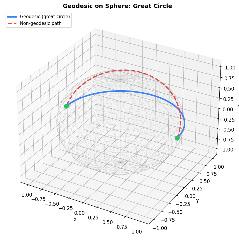
2.2 Geodesics on a Sphere

A geodesic on a sphere of radius \(R\) is the curve of shortest length joining two points on the surface. Parametrizing by \(\phi\) (latitude) and \(\theta\) (longitude), the length functional is

\[J(\phi, \theta) = R \int_0^1 \sqrt{\sin^2(\phi(t))\dot{\theta}(t)^2 + \dot{\phi}(t)^2}\,dt.\]

By orienting the sphere so that one point is at the north pole and both points share the same meridian, the problem simplifies dramatically. Setting \(\theta(t) = \theta_B\) (constant), any smooth \(\phi\) connecting the two latitudes achieves the minimum length \(R\phi_B\). This is a great circle arc, confirming that geodesics on spheres are arcs of great circles.

2.3 The Gateaux Derivative

The analogue of the directional derivative in a linear space is the Gateaux derivative.

Definition 2.7. For \(J : D \subseteq Y \to \mathbb{R}\) and \(y, v \in D\), the Gateaux derivative (or variation) is

\[\delta J(y; v) = \lim_{\epsilon \to 0} \frac{J(y + \epsilon v) - J(y)}{\epsilon},\]

when it exists. If \(\frac{\partial}{\partial \epsilon} J(y + \epsilon v)\) exists and is continuous at \(\epsilon = 0\), it can be computed as

\[\delta J(y; v) = \left.\frac{\partial}{\partial \epsilon} J(y + \epsilon v)\right|_{\epsilon = 0}.\]

For the arc-length functional \(J(y) = \int_0^5 \sqrt{1 + (y')^2}\,dx\), this formula gives

\[\delta J(y; v) = \int_0^5 2y'(x)v'(x)\,dx.\]

2.4 Convex Functionals

The definitions and key theorems from \(\mathbb{R}^n\) carry over verbatim to general linear spaces.

Definition 2.11 (Convex functional). \(J : Y \to \mathbb{R}\) is convex on \(D \subseteq Y\) if for all \(y, x \in D\) and \(0 < \alpha < 1\),

\[J(y + \alpha(x - y)) \leq \alpha J(x) + (1 - \alpha)J(y).\]

Definition 2.14 (Stationary point of a functional). If \(\delta J(y^*; v) = 0\) for all admissible variations \(v\), then \(y^*\) is a stationary point of \(J\).

Proposition 2.15. If \(J\) is convex on \(D\), then every stationary point \(y_0 \in D\) minimizes \(J\) on \(D\). If \(J\) is strictly convex, the minimizing element is unique. This is the infinite-dimensional analogue of Theorem 1.16 and is proved identically: convexity implies \(J(y) \geq J(y_0) + \delta J(y_0; y - y_0) = J(y_0)\) for all \(y \in D\).

---

The Euler–Lagrange Equation

3.1 Derivation

Consider the fundamental class of functionals of the form

\[J(y) = \int_a^b f(x, y(x), y'(x))\,dx,\]

where \(f : \mathbb{R}^3 \to \mathbb{R}\). The function \(f\) is called the Lagrangian (in honour of Lagrange’s contributions). Many classical problems — geodesics, brachistochrone, minimal surfaces — take this form.

Theorem 3.1 (Gateaux derivative of J). Assuming \(f, f_y, f_z\) are continuous on \([a,b] \times D\) (where \(z = y'\), the Gateaux derivative is

\[\delta J(y; v) = \int_a^b \left[f_y(x, y, y')v(x) + f_z(x, y, y')v'(x)\right]dx.\]

For stationary functions over the set \(D = \{y \in C^1[a,b] : y(a) = y_a,\, y(b) = y_b\}\), admissible variations must satisfy \(v(a) = v(b) = 0\).

Integrating by parts on the second term and using the boundary conditions, the Gateaux derivative becomes

\[\delta J(y; v) = \int_a^b \left[f_y[y(x)] - \frac{d}{dx}f_z[y(x)]\right]v(x)\,dx.\]

Theorem 3.5 (Euler–Lagrange). A function \(y\) is a stationary function of \(J\) on \(D\) if and only if it satisfies the Euler–Lagrange equation:

\[\frac{d}{dx} f_z[y(x)] = f_y[y(x)].\]

The “if” direction (Proposition 3.2) follows immediately from the integration-by-parts computation above. The “only if” direction requires the du Bois-Reymond Lemma and Lemma 3.4, which together show that any function making \(\delta J(y; v) = 0\) for all admissible \(v\) must satisfy the Euler–Lagrange equation.

Lemma 3.3 (du Bois-Reymond). If \(h \in C[a,b]\) and \(\int_a^b h(x)v'(x)\,dx = 0\) for all \(v \in A\), then \(h\) is constant on \([a,b]\).

3.2 Simplifications

If \(f\) is missing one of its arguments, the Euler–Lagrange equation simplifies considerably:

1. \(f\) independent of \(y'\): The equation becomes \(f_y = 0\), an algebraic equation rather than a differential equation.

2. \(f\) independent of \(y\): \(f_y = 0\), so the equation becomes \(\frac{d}{dx}f_z = 0\), or \(f_z = c\) (constant). This first integral is easier to solve.

3. \(f\) independent of \(x\) (Beltrami identity): If \(y \in C^2[a,b]\), any stationary function satisfies

\[f(y, y') - y' f_z(y, y') = \text{constant}.\]

This is a first-order equation, significantly easier to solve than the general second-order Euler–Lagrange equation.

3.3 Pointwise Convexity

Definition 3.10. The function \(f : \mathbb{R}^3 \to \mathbb{R}\) is pointwise convex on \(S\) if \(f, f_y, f_z\) are continuous and

\[f(x, y+v, z+w) - f(x, y, z) - f_y v - f_z w \geq 0\]

for all perturbations \((v, w)\). Note that \(x\) is held fixed, so a convex function is also pointwise convex, but not necessarily vice versa.

Theorem 3.13. If \(f\) is pointwise convex, then the functional \(J(y) = \int_a^b f[y]\,dx\) is convex on \(D = \{y \in C^1[a,b] : y(a) = y_a,\, y(b) = y_b, (y(x), y'(x)) \in D\}\). Strict pointwise convexity gives strict convexity of \(J\).

Proposition 3.15. If \(f = f(x, z)\) (independent of \(y\) and \(f_{zz}(x, z) > 0\) for all \(x\), then \(J\) is strictly convex. The proof uses Taylor’s remainder theorem to show \(f(x, z+w) > f(x,z) + f_z(x,z)w\).

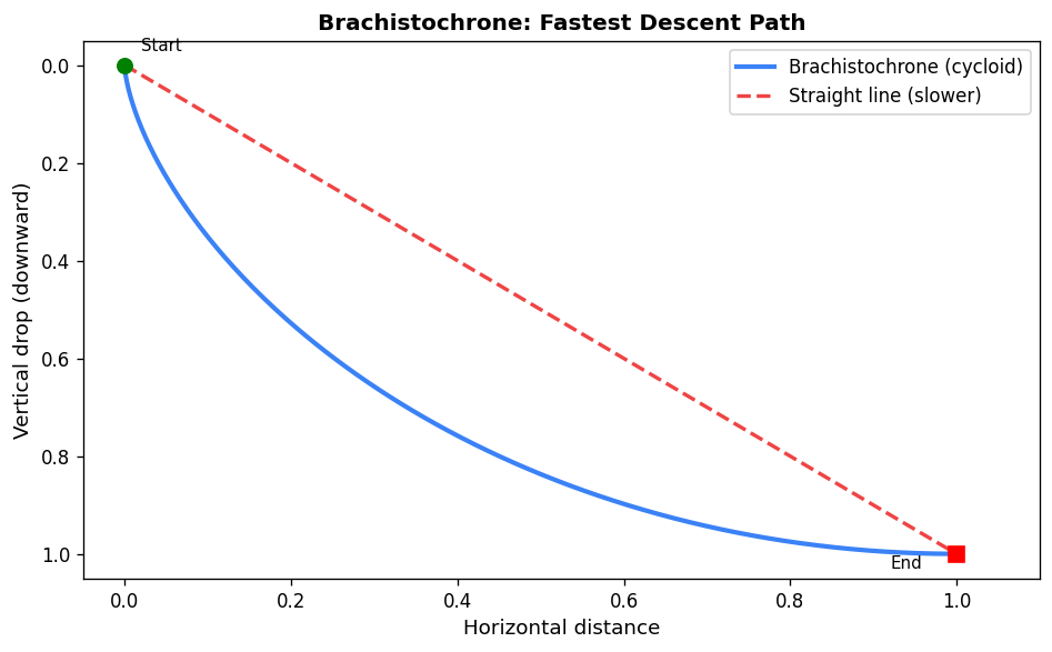
3.4 The Brachistochrone Problem

The brachistochrone asks: what path minimizes the travel time for a bead sliding under gravity (frictionlessly) between two points? This historical problem, solved by Bernoulli in 1696, was the founding problem of the calculus of variations.

Reversing the standard coordinate system so that \(x\) is vertical and \(y\) horizontal, conservation of energy gives \(v = \sqrt{2gx}\), and the travel time functional becomes

\[T(y) = \int_0^a \frac{\sqrt{1 + (y'(x))^2}}{\sqrt{2gx}}\,dx.\]

Since \(f_{zz}(x,z) = \frac{1}{(2gx)^{1/2}(1+z^2)^{3/2}} > 0\) for \(x > 0\), Proposition 3.15 implies \(T\) is strictly convex, so the unique stationary function minimizes \(T\).

Since \(f\) is independent of \(y\), the Euler–Lagrange equation reduces to \(f_z = c\):

\[\frac{y'}{\sqrt{x}\sqrt{1+(y')^2}} = c.\]

Solving this via the substitution \(x(\theta) = \frac{k^2}{2}(1 - \cos \theta)\) leads to the parametric solution

\[x(\theta) = \frac{k^2}{2}(1-\cos\theta), \quad y(\theta) = \frac{k^2}{2}(\theta - \sin\theta).\]

This curve is a cycloid — the path traced by a point on the rim of a rolling circle. The constant \(k\) is determined by the endpoint \((a, b)\).

---

Extensions and Generalizations

4.1 Natural Boundary Conditions

When not all boundary conditions are prescribed, the variational problem determines the missing conditions automatically. Suppose \(y(a) = y_a\) is fixed but \(y(b)\) is free. Admissible variations satisfy \(v(a) = 0\) but \(v(b)\) is free. Integration by parts on \(\delta J(y;v)\) yields a boundary term \(f_z[y(b)]v(b)\) in addition to the Euler–Lagrange integral.

Theorem 4.2. A function \(y\) is stationary for \(J\) on \(D_1 = \{y \in C^1[a,b] : y(a) = y_a\}\) if and only if it satisfies the Euler–Lagrange equation and the natural boundary condition

\[f_z[y(b)] = 0.\]

Example 4.3 (Steady-state temperature). A bar of length \(L\) with one end fixed at \(y(0) = 100\) and the other free minimizes \(U(y) = k \int_0^L (y')^2\,dx\). The natural boundary condition \(f_z[y(L)] = 2ky'(L) = 0\) means no heat flux at the free end. Together with the Euler–Lagrange equation \(y'' = 0\), the unique solution is \(y(x) = 100\) (constant temperature).

If neither endpoint is specified (Theorem 4.4), the natural boundary conditions become \(f_z[y(a)] = f_z[y(b)] = 0\), and the minimizing function is unique up to an additive constant when \(f\) is strictly pointwise convex.

4.2 Variable Endpoint Problems and Transversality

When the endpoint \(b\) is free and \(y(b)\) must lie on a given curve \(\varphi(x)\), both the function and the endpoint vary. Introducing the conjugate momentum \(p[y(x)] = f_z[y(x)]\) and the Hamiltonian \(H[y(x)] = -f[y(x)] + y'(x)f_z[y(x)]\), the stationarity condition yields:

Theorem 4.7 (Transversality condition). A stationary function satisfies the Euler–Lagrange equation and the transversality condition

\[H[y(b)] = p[y(b)]\varphi'(b),\]

i.e., \(-f[y(b)] + y'(b)f_z[y(b)] = f_z[y(b)]\varphi'(b)\). Geometrically, this means the optimal curve meets the target curve \(\varphi\) perpendicularly in the appropriate metric.

For the brachistochrone landing on a curve, this condition implies the cycloid is orthogonal to the landing curve at the point of contact.

4.3 Higher-Order Derivatives

Some physical problems involve second derivatives. The potential energy of a beam under load \(p(x)\) and small deflection \(y(x)\) is

\[U(y) = \int_0^L \frac{\mu}{2}(y''(x))^2 - p(x)y(x)\,dx.\]

For functionals \(J(y) = \int_a^b f(x, y, y', y'')\,dx\) with fully specified boundary conditions, integration by parts twice yields the generalized Euler–Lagrange equation:

\[f_y[y] - \frac{d}{dx}f_z[y] + \frac{d^2}{dx^2}f_w[y] = 0\]

where \(z = y', w = y''\). For the beam problem with both ends clamped, this gives \(\mu y'''' = p(x)\), which under uniform load \(p = \mu F\) integrates to \(y(x) = \frac{F}{24}x^2(x-L)^2\).

4.4 Broken Extremals (Weierstrass–Erdmann Conditions)

In some problems, no smooth stationary function exists and the minimum is achieved by piecewise smooth functions (functions in \(\hat{C}^1[a,b]\) with finitely many corners). By treating a corner \(c\) as a variable endpoint lying on an arbitrary curve, one derives the Weierstrass–Erdmann corner conditions: at any corner, both

\[p[y(c^-)] = p[y(c^+)] \quad \text{and} \quad H[y(c^-)] = H[y(c^+)]\]

must hold. That is, the conjugate momentum \(f_z\) and the Hamiltonian \(H = -f + y'f_z\) are both continuous at corners, even though \(y'\) is not. A necessary condition for a corner to exist is that \(f_{zz} = 0\) at some point.

---

Hamilton’s Principle

5.1 Background and Statement

The success of the calculus of variations in solving mechanical problems like the brachistochrone inspired scientists to seek a variational principle governing the motion of all physical systems. Work of Lagrange, Euler, Poisson, and Hamilton culminated in Hamilton’s Principle.

Definition 5.1 (Potential). A potential is a scalar quantity whose negative gradient gives the force acting on a body.

Definition 5.2 (Action integral). The action integral is

\[A(y) = \int_a^b L(t, y, \dot{y})\,dt,\]

where the Lagrangian \(L = T - U\) is the difference between kinetic energy \(T\) and potential energy \(U\).

Hamilton’s Principle of Stationary Action. Between fixed times \(a\) and \(b\), a physical system moves along the trajectory that makes the action integral stationary over all admissible trajectories.

5.2 Newton’s Laws from Hamilton’s Principle

Example 5.3 (Cart). For a cart of mass \(m\) with potential energy \(U(y)\), the Lagrangian is \(L = \frac{1}{2}m\dot{y}^2 - U(y)\). The Euler–Lagrange equation \(L_y - \frac{d}{dt}L_{\dot{y}} = 0\) gives \(-U_y - m\ddot{y} = 0\), i.e., \(m\ddot{y} = -U_y\). Since \(-U_y\) is the force on the cart, this is Newton’s Second Law, \(F = ma\).

Example 5.4 (Spring-mass). With \(T = \frac{1}{2}m\dot{y}^2\) and \(U = \frac{1}{2}ky^2\), the Euler–Lagrange equation yields \(m\ddot{y} = -ky\), the familiar harmonic oscillator equation.

5.3 Multi-Variable Euler–Lagrange and Conservation of the Hamiltonian

When the system has multiple degrees of freedom, \(y = (y_1, \ldots, y_n)\), stationarity of the action requires an Euler–Lagrange equation for each component:

Theorem 5.5. A function \(y \in (C^1[a,b])^n\) is stationary for \(J\) if and only if

\[f_{y_i}[y(x)] - \frac{d}{dx}f_{z_i}[y(x)] = 0, \quad i = 1, \ldots, n.\]

When \(L\) does not depend explicitly on time, energy is conserved:

Theorem 5.6 (Conservation of the Hamiltonian). If \(L\) is independent of \(t\), then the Hamiltonian

\[H = -L + \sum_{i=1}^n \dot{y}_i L_{\dot{y}_i}\]

is constant along stationary trajectories. This is the law of conservation of energy.

5.4 Generalized Coordinates

A key advantage of Lagrangian mechanics is the freedom to use any convenient coordinate system. Generalized coordinates are an independent minimal set \(q = (q_1, \ldots, q_n)\) describing the system configuration.

Example 5.8 (Pendulum). In Cartesian coordinates, a pendulum of length \(\ell\) has constraint \(x^2 + y^2 = \ell^2\). Using the angle \(\theta\) as a single generalized coordinate: \(T = \frac{1}{2}m\ell^2\dot{\theta}^2\), \(U = -mg\ell\cos\theta\), and the Euler–Lagrange equation gives

\[\ddot{\theta} = -\frac{g}{\ell}\sin\theta.\]

Example 5.10 (Spring-pendulum). A mass on a spring of length \(r\) at angle \(\theta\) from vertical uses generalized coordinates \((r, \theta)\). The Lagrangian is

\[L = \frac{1}{2}m(\dot{r}^2 + r^2\dot{\theta}^2) - \frac{1}{2}k(r-r_0)^2 + mg(r_0 - r\cos\theta),\]

yielding the coupled equations \(\ddot{r} - \dot{\theta}^2 r = -\frac{k}{m}(r-r_0) + g\cos\theta\) and \(2\dot{r}\dot{\theta} + r\ddot{\theta} = -g\sin\theta\).

Hamilton’s Principle (Revised). Between fixed times, a physical system follows the generalized trajectory \(q \in (C^1[a,b])^n\) that makes stationary the action \(A(q) = \int_a^b L(t, q, \dot{q})\,dt\).

5.5 Kepler’s Laws from Hamilton’s Principle

For two bodies with gravitational potential \(U = -k/r\) in polar coordinates \((r, \theta)\), the Lagrangian is

\[L(r, \theta) = \frac{1}{2}m(\dot{r}^2 + r^2\dot{\theta}^2) + \frac{k}{r}.\]

The Euler–Lagrange equation for \(\theta\) gives \(\frac{d}{dt}(mr^2\dot{\theta}) = 0\), i.e., angular momentum is conserved — from which equal areas are swept in equal times (Kepler’s Second Law).

Combining with conservation of the Hamiltonian and solving the resulting separable ODE for \(r(\theta)\) leads to the conic section

\[r(\theta) = \frac{c}{1 + \varepsilon \cos(\theta - \theta_0)},\]

where \(\varepsilon < 1\) gives an ellipse — Kepler’s First Law. The period-axis relationship \(T^2 \propto a^3\) follows from the area formula — Kepler’s Third Law.

---

Hamilton’s Principle (Continued)

6.1 Canonical Equations

Hamilton’s Principle yields \(n\) coupled second-order ODEs. A standard technique converts these to \(2n\) first-order equations using canonical variables.

Define the canonical momenta \(p_i = L_{\dot{q}_i}\). For the general case with Lagrangian \(L = \frac{1}{2}\dot{q}^T A(q)\dot{q} - U(t,q)\) where \(A\) is positive definite:

Writing \(p = A(q)\dot{q}\) (so \(\dot{q} = A^{-1}p\), the Hamiltonian expressed in terms of \((q, p)\) is

\[H(t, q, p) = \sum_i p_i \dot{q}_i - L = \frac{1}{2}p^T A^{-1}(q)p + U(t, q).\]

The canonical equations of motion (Hamilton’s equations) are then:

\[\dot{q}_i = \frac{\partial H}{\partial p_i}, \quad \dot{p}_i = -\frac{\partial H}{\partial q_i}, \quad i = 1, \ldots, n.\]

Note the elegant symmetry: the equations for \(q\) and \(p\) differ only by a sign. This structure is central to the connection with optimal control theory.

Example 6.1 (Pendulum). With \(L = \frac{1}{2}m\ell^2\dot{\theta}^2 - mg\ell(1-\cos\theta)\) and \(p = m\ell^2\dot{\theta}\), the Hamiltonian is \(H = \frac{p^2}{2m\ell^2} + mg\ell(1-\cos\theta)\). The canonical equations reproduce the pendulum ODE.

6.2 Multiple Spatial Variables

Hamilton’s Principle extends to problems where the unknown function depends on multiple variables. For a functional

\[J(y) = \int_D f(\tilde{x}, y(\tilde{x}), \nabla y(\tilde{x}))\,d\tilde{x}\]

over a bounded domain \(D \subseteq \mathbb{R}^n\) with fixed boundary values, the Divergence Theorem (the multi-dimensional integration by parts) gives:

Euler–Lagrange PDE:

\[f_y[y(\tilde{x})] - \nabla \cdot f_{\nabla y}[y(\tilde{x})] = 0.\]

Example 6.4. The potential energy \(U(y) = \frac{k}{2}\int_D |\nabla y|^2\,d\tilde{x}\) (thermal diffusion) is minimized when \(\nabla^2 y = 0\) — Laplace’s equation.

For a vibrating string with both spatial and temporal dependence, the action functional \(A(y) = \int_a^b \int_0^\ell \frac{1}{2}\rho y_t^2 - \frac{1}{2}\tau y_x^2\,dx\,dt\) (linearized approximation) yields the wave equation:

\[\rho \frac{\partial^2 y}{\partial t^2} = \tau \frac{\partial^2 y}{\partial x^2}.\]

---

Some Complexities

7.1 Lack of Convexity and Existence of Minima

Convexity has been central to our analysis: for a convex functional, every stationary point is a global minimum. When convexity fails, a stationary function may be only a local minimum or even a saddle point. Moreover, the functional analogue of the Extreme Value Theorem requires compactness, which in infinite-dimensional function spaces is a much stronger requirement than mere closedness and boundedness. The following example illustrates both issues.

7.2 Minimum Surface of Revolution

Find a curve joining two points so that the surface formed by revolving it around the \(x\)-axis has minimal area. Normalizing the left endpoint to \((0,1)\) and the right to \((x_1, y_1)\), the cost is

\[J(y) = 2\pi \int_0^{x_1} y(x)\sqrt{1 + (y'(x))^2}\,dx.\]

Since \(f = 2\pi y\sqrt{1+z^2}\) is independent of \(x\), the Beltrami identity gives \(f - y'f_z = c\), simplifying to

\[\frac{dy}{dx} = \sqrt{\frac{y^2 - c^2}{c^2}}.\]

This separable equation integrates to a catenary \(y(x) = c \cosh\!\left(\frac{x+d}{c}\right)\).

Imposing \(y(0) = 1\) and \(y(x_1) = y_1\) leads to a transcendental equation for the constants. The striking result is that for any given endpoint, there may be two solutions, one, or none — unlike previous problems which always had a unique solution. When two exist, one (with \(d > 0\) is a local minimum; the other is a saddle point. When none exist (when \(x_1\) is large relative to \(y_1\), no smooth minimizer exists: the infimum is approached by a sequence of functions converging to two disconnected disks, known as the Goldschmidt discontinuous solution.

---

Problems with Constraints

8.1 Integral Constraints

Consider minimizing \(J(y) = \int_a^b f[y]\,dx\) subject to an integral constraint \(G(y) = \int_a^b g[y]\,dx = c\). By analogy with Lagrange multipliers in finite dimensions, introduce the augmented functional

\(\tilde{J}(y) = \int_a^b \(f[y] + \lambda g[y]\),dx)

for some constant \(\lambda\). The multiplier theorem (Theorem 8.2) guarantees that a minimizer \(y_o\) of \(\tilde{J}\) minimizes \(J\) subject to the constraint, with \(\lambda\) determined by the constraint \(G(y_o) = c\).

The corresponding Euler–Lagrange equation for the augmented problem is

\[\frac{d}{dx}(f + \lambda g)_z[y] = (f + \lambda g)_y[y],\]

which has three constants: two integration constants and \(\lambda\), determined by the two boundary conditions and the constraint.

Example 8.6 (Simplified Dido’s Problem). Minimize \(\int_{-1}^1 y\,dx\) over curves with \(y(-1) = y(1) = 0\) and length \(\int_{-1}^1\sqrt{1+(y')^2}\,dx = \pi\). The augmented Lagrangian is \(\tilde{f} = y + \lambda\sqrt{1+(y')^2}\). The Beltrami identity and parametric analysis yield the stationary functions \(x = \sin\theta, y = -\cos\theta\) and its reflection — both are semicircles. The one below the axis is the minimum of the augmented problem, confirming that among curves of fixed length with endpoints on the \(x\)-axis, the semicircle encloses maximum area — the classical isoperimetric inequality.

Example 8.7 (General Dido’s Problem). For a straight shore, the curve of fixed length \(L\) enclosing maximum inland area is a semicircle of radius \(b = L/\pi\). The natural boundary conditions at the free endpoints (where the curve meets the shore) combine with the Beltrami identity to select the circular arc.

8.2 Non-Integral Constraints and Optimal Control

The most important class of constrained problems involves a differential equation constraint. With independent variable \(t\) and additional function \(u(t)\) (the control), the problem is:

Minimize \(J(y,u) = \int_0^T f(t, y, u)\,dt\\) subject to \(\dot{y}(t) = g(t, y, u)\\).

The function \(y\) is the state, determined by the ODE given \(u\). The function \(u\) is the control, freely chosen to minimize the cost. This is the central formulation of optimal control theory.

Example 8.9 (Energy-optimal control of a rigid body). Move a body from \((w(0), \dot{w}(0)) = (w_0, 0)\) to rest \((w(T), \dot{w}(T)) = (0, 0)\) while minimizing \(\int_0^T u^2\,dt\) subject to \(\ddot{w} = u\). Setting \(y_1 = w, y_2 = \dot{w}\) and substituting \(u = \ddot{w}\) into the Euler–Lagrange equation for \(J(w) = \int_0^T \ddot{w}^2\,dt\) gives \(w^{(4)} = 0\), so \(w(t) = \frac{a}{6}t^3 + \frac{b}{2}t^2\). Boundary conditions determine \(a\) and \(b\), and the optimal control is the linear ramp \(u(t) = at + b\).

---

Introduction to Optimal Control

9.1 The Augmented Problem

The general optimal control problem is to minimize

\[J(y, u) = \int_0^T f(t, y, u)\,dt\]

subject to \(\dot{y} = g(t, y, u)\) and boundary conditions on \(y\). Introducing a vector of Lagrange multiplier functions (the adjoint variables or costates) \(p(t) \in \mathbb{R}^n\), form the augmented cost

\[\tilde{J}(y, u, p) = \int_0^T \left[f(t, y, u) + p(t)^T(\dot{y}(t) - g(t, y, u))\right]\,dt.\]

Theorem 9.1 (Optimality equations). A triple \((y, u, p)\) is stationary for \(\tilde{J}\) if and only if:

\[\dot{p} = f_y^T - g_y^T p \quad \text{(adjoint equation)},\]\[\dot{y} = g(t, y, u) \quad \text{(state equation)},\]\[f_u^T - p^T g_u = 0 \quad \text{(optimality condition)}.\]

If only \(y(0) = y_0\) is specified (free final state), the adjoint boundary condition is \(p(T) = 0\).

9.2 The Hamiltonian Reformulation

Define the control Hamiltonian

\[H(t, y, p, u) = f(t, y, u) + p^T g(t, y, u).\]

The three optimality equations take the elegant canonical form:

\[\dot{p}_i = -\frac{\partial H}{\partial y_i}, \quad \dot{y}_i = \frac{\partial H}{\partial p_i}, \quad \frac{\partial H}{\partial u_j} = 0.\]

These are strikingly similar to Hamilton’s canonical equations from mechanics. The third equation, \(H_u = 0\), says that the optimal control makes the Hamiltonian stationary with respect to \(u\).

Example 9.5. For the system \(\dot{y} = -y + u\) with cost \(\int_0^T \frac{1}{2}u^2\,dt\), boundary conditions \(y(0) = 1, y(T) = 2\): the Hamiltonian is \(H = \frac{1}{2}u^2 + p(-y+u)\). The adjoint equation gives \(\dot{p} = p\), so \(p(t) = ce^t\). The condition \(H_u = u + p = 0\) gives the optimal control \(u^o(t) = -p(t) = -ce^t\). Substituting into the state equation and applying boundary conditions determines \(c\).

Theorem 9.9. The Hamiltonian \(H\) is pointwise convex in \((y, u)\) if and only if \(\tilde{f}\) is pointwise convex. In particular, if \(f\) is convex and \(g\) is linear, then \(H\) is convex, and every solution of the optimality equations provides a global minimum.

---

Pontryagin’s Maximum Principle

10.1 The Limitation of Unconstrained Controls

When the Hamiltonian is linear in \(u\), the condition \(H_u = 0\) gives no information about the optimal control. This arises naturally in minimum-time problems where the cost is simply \(\int_0^T dt\) with \(f = 1\). The fundamental resolution is to explicitly constrain the control to a closed set \(U\) and replace stationarity with maximization of the Hamiltonian over \(U\).

10.2 Pontryagin’s Maximum Principle

Theorem 10.2 (Pontryagin’s Maximum Principle, PMP). Consider minimizing \(J(y, u) = \int_0^T f(t, y, u)\,dt\) subject to \(\dot{y} = g(t, y, u)\) with \(u(t) \in U \subseteq \mathbb{R}^m\) (U closed). If \(u^o, y^o\) are optimal, there exists an adjoint function \(p(t)\) satisfying

\[\dot{p}_i = -\frac{\partial H}{\partial y_i},\]

with Hamiltonian

\[H(t, y, p, u) = p^o f(t, y, u) + \sum_{i=1}^n p_i(t)g_i(t, y, u),\]

such that \((p^o, p(t)) \neq (0, 0)\) for all \(t\), and \(H\) is maximized with respect to \(u\) at \(u^o(t)\) for every \(t\).

For non-degenerate problems, \(p^o = 1\), recovering \(H = f + p^T g\). When \(H\) is convex (Corollary 10.3), every solution of the PMP equations provides a global minimum.

The PMP provides necessary conditions. It was introduced to handle cases where the optimality condition \(H_u = 0\) fails — particularly when \(u\) is constrained or \(H\) is linear in \(u\).

10.3 Time-Optimal Control

Example 10.6 (First-order system). Minimize time to drive \(\dot{y} = u\) from \(y(0) = 1\) to \(y(T) = 0\) with \(|u| \leq M\). The Hamiltonian is \(H = -1 + pu\). Maximizing over \(u\): \(u^o = M\,\text{sgn}(p)\). The adjoint equation \(\dot{p} = 0\) gives constant \(p\), so \(u^o = \pm M\) throughout. Starting from \(y(0) = 1 > 0\), the optimal strategy is \(u^o = -M\), reaching zero in time \(T = 1/M\).

Example 10.7 (Double integrator). Minimize time to drive \(\ddot{w} = u\) with \(|u| \leq 1\) to \((w(T), \dot{w}(T)) = (0,0)\). With \((y_1, y_2) = (w, \dot{w})\), the Hamiltonian is \(H = -1 + p_1 y_2 + p_2 u\). The optimal control \(u^o = \text{sgn}(p_2)\); since \(p_2(t) = at + b\) is linear, there is at most one switch. The switching curve \(y_1 = \pm\frac{1}{2}y_2^2\) (with sign depending on \(y_2\) divides the phase plane: the optimal control is \(-1\) above and \(+1\) below. For \((y_1(0), y_2(0)) = (1, 0)\), the optimal control is \(u = -1\) until \(t = 1\), then \(u = +1\), reaching the origin at \(T = 2\).

10.4 Bang-Bang Control

When \(H\) is linear in \(u\) and \(U = [M_1, M_2]\), the optimal control always takes the extreme values:

\[u^o_k(t) = \begin{cases} M_1 & \text{if } p(t)^T B_k < 0, \\\ M_2 & \text{if } p(t)^T B_k > 0. \end{cases}\]

Such a control is called bang-bang.

Theorem 10.8. For the linear time-optimal problem \(\dot{y} = Ay + Bu\), if the vectors \(B_k, AB_k, \ldots, A^{n-1}B_k\) are linearly independent, then the optimal control \(u^o_k\) is bang-bang.

Theorem 10.9. If all eigenvalues of \(A\) are real, the bang-bang control has at most \(n-1\) switches. If eigenvalues are complex, switches can occur arbitrarily often (as in the harmonic oscillator).

Proof sketch: The switching function \(\sigma(t) = p(t)^T B_k\) satisfies \(\sigma(t) = \sum_j \alpha_j e^{\lambda_j t}\) (a sum of \(n\) exponentials). Lemma 10.10 shows that a sum of \(n\) exponentials with distinct real exponents has at most \(n-1\) zeros, bounding the number of switches.

Example 10.11 (Harmonic oscillator). For \(\ddot{w} + w = u\) with \(|u| \leq 1\), the eigenvalues of \(A\) are \(\pm i\) (complex), so there is no bound on switches. The adjoint \(p_2(t) = M\cos(t + \phi)\) leads to switches at intervals of \(\pi\). Optimal trajectories follow arcs of circles centered at \((\pm 1, 0)\) in the phase plane, switching direction at the switching curve (a series of semicircles in the second and fourth quadrants).

---

Linear Quadratic Control

11.1 Finite-Time LQR

The Linear Quadratic Regulator (LQR) is the most important solved problem in optimal control. It combines linear dynamics with a quadratic cost, admitting a complete analytical solution.

Consider the linear time-invariant system

\[\dot{y}(t) = Ay(t) + Bu(t), \quad y(0) = y_0,\]

with \(A \in \mathbb{R}^{n\times n}\), \(B \in \mathbb{R}^{n \times m}\). The quadratic cost

\[J(u; T) = \int_0^T \left[y(t)^T Q y(t) + u(t)^T R u(t)\right]\,dt\]

penalizes both state deviation and control effort, where \(Q = C^T C \geq 0\) and \(R = E^T E > 0\) are symmetric weighting matrices.

Applying the optimality equations (Theorem 9.1) and defining \(z = -p/2\), the optimal control is

\[u^o(t) = -R^{-1} B^T z(t)\]

where \(z\) satisfies \(\dot{z} = -A^T z - Qy\) with \(z(T) = 0\). The difficulty is that \(z(t)\) depends on future state values. The key insight is to express the adjoint as a linear function of the current state.

Theorem 11.3 (Differential Riccati Equation). Define \(P(t; T)\) by \(z(t) = P(t;T)y^o(t)\). Then \(P(t;T)\) satisfies the Differential Riccati Equation (DRE):

\[\dot{P}(t;T) + A^T P + P A - P B R^{-1} B^T P + Q = 0, \quad P(T;T) = 0,\]

and the optimal feedback control is

\[u^o(t) = -R^{-1} B^T P(t;T) y^o(t).\]

The minimum cost is \(J(u^o; T) = y_0^T P(0;T) y_0\). Furthermore, \(0 \leq P(0;T) < \infty\) for all \(T\).

The DRE is solved backward in time from \(P(T;T) = 0\) to \(P(0;T)\). The optimal control is a linear state feedback law — the control at each time depends only on the current state, not on future states. This closed-loop structure makes the controller self-correcting and practical to implement.

11.2 Infinite-Horizon LQR and the Algebraic Riccati Equation

The infinite-horizon LQR problem seeks to minimize

\[J = \int_0^{\infty} \left[x(t)^T Q x(t) + u(t)^T R u(t)\right]\,dt\]

subject to \(\dot{x} = Ax + Bu\), where the goal is to stabilize the system (drive \(x(t) \to 0\) as \(t \to \infty\).

Lemma 11.1. For any symmetric matrix \(P\), the functional \(V(x(\cdot), u(\cdot)) = -\int_0^\infty [(Ax+Bu)^T Px + x^T P(Ax+Bu)]\,dt\) depends only on \(x_0 = x(0)\) (provided \(x(t) \to 0\), with value \(V = x_0^T P x_0\).

The trick is to complete the square in the cost. Writing the cost as

\[J = V + \int_0^\infty \left[x^T(A^T P + PA + Q)x + u^T Ru + 2u^T B^T Px\right]\,dt,\]

and noting that \(u^T Ru + 2u^T B^T Px = (u - Kx)^T R(u-Kx) - (Kx)^T R(Kx)\) with \(K = -R^{-1}B^T P\), we get

\[J = x_0^T P x_0 + \int_0^\infty \left[x^T(A^T P + PA + Q - PBR^{-1}B^T P)x + (u - Kx)^T R(u-Kx)\right]\,dt.\]

If \(P\) satisfies the Algebraic Riccati Equation (ARE):

\[A^T P + PA + Q - PBR^{-1}B^T P = 0,\]

and \(A - BR^{-1}B^T P\) is Hurwitz (all eigenvalues with negative real parts), then the cost reduces to \(J = x_0^T P x_0\) with the feedback law \(u = Kx\), and this is optimal among all stabilizing controllers.

Theorem 11.2. Suppose the ARE admits a symmetric positive semi-definite solution \(P\) such that \(A - BR^{-1}B^T P\) is Hurwitz. Then the feedback law \(u = Kx = -R^{-1}B^T Px\) stabilizes the system and minimizes the LQR cost, with optimal cost \(J^* = x_0^T P x_0\).

The ARE is the equilibrium condition of the DRE: \(\dot{P} = 0\). Under appropriate conditions (stabilizability and detectability), the DRE solution \(P(t; T)\) converges as \(T \to \infty\) to the stabilizing solution of the ARE.

Example 11.3. For \(x' = u\) with cost \(J = \int_0^\infty u^2\,dt\): the ARE is \(-P^2 = 0\), so \(P = 0\) and \(u = 0\). This is not stabilizing (the uncontrolled system is neutrally stable, not asymptotically stable). Any stabilizing control \(u = -\varepsilon x\) gives cost \(\frac{\varepsilon x_0^2}{2} \to 0\) as \(\varepsilon \to 0\), but the infimum is not attained by a stabilizing controller.

Example 11.4. For \(x' = x + u\) with cost \(\int_0^\infty u^2\,dt\): the ARE is \(2P - P^2 = 0\), giving \(P = 0\) (not stabilizing) or \(P = 2\) (stabilizing). The optimal control \(u = -2x\) gives closed-loop system \(x' = -x\) and optimal cost \(J^* = 2x_0^2\).

Example 11.5 (Double integrator). For \(y'' = u\) with output \(y = x_1\), written as

\[A = \begin{pmatrix} 0 & 1 \\\ 0 & 0 \end{pmatrix}, \quad B = \begin{pmatrix} 0 \\\ 1 \end{pmatrix}, \quad Q = \begin{pmatrix} 1 & 0 \\\ 0 & 0 \end{pmatrix}, \quad R = r > 0,\]

the ARE can be solved manually. Setting \(P = \begin{pmatrix} p_1 & p_2 \\\ p_2 & p_3 \end{pmatrix}\), the three scalar equations yield

\[p_2 = \sqrt{r}, \quad p_1 = \frac{1}{r}p_2 p_3 = (2r)^{1/4}\sqrt{r}\^{1/2}, \quad p_3 = (2r)^{3/4},\]

and the optimal gain \(K = -R^{-1}B^T P = -\frac{1}{r}[p_2 \;\; p_3] = -[r^{-1/2}, (2/r)^{1/4} r^{-3/4}]\). The closed-loop characteristic polynomial \(s^2 + (2/r)^{1/4}s + 1/\sqrt{r} = 0\) has both roots with negative real parts, confirming asymptotic stability.

11.3 Summary of the LQR Design Procedure

Step	Action
1	Formulate system \(\dot{x} = Ax + Bu\) and choose weighting matrices \(Q \geq 0\), \(R > 0\)
2	Solve the ARE \(A^T P + PA + Q - PBR^{-1}B^T P = 0\) for the symmetric positive semi-definite solution \(P\)
3	Compute feedback gain \(K = -R^{-1}B^T P\)
4	Implement \(u(t) = Kx(t)\) — this stabilizes the system with cost \(J^* = x_0^T P x_0\)

In MATLAB, the optimal gain is returned by lqr(A, B, Q, R). The choice of \(Q\) and \(R\) is a design decision reflecting the trade-off between state regulation performance and control effort.

---

Course Summary

This course developed the complete arc from finite-dimensional optimization to optimal control of dynamical systems:

Topic	Key Result
Finite-dim optimization	Gradient = 0 at stationary points; convexity guarantees global minima
Functional calculus	Gateaux derivative on linear spaces; stationarity in function spaces
Euler–Lagrange equation	Necessary and sufficient condition for stationary functions
Simplifications	Beltrami identity, natural BCs, transversality
Hamilton’s Principle	Action stationarity yields all of classical mechanics
Canonical equations	Hamilton’s equations; connection to optimal control
Constrained problems	Lagrange multipliers, isoperimetric inequality (Dido’s problem)
Optimal control	Adjoint state, Hamiltonian, two-point boundary value problem
Pontryagin’s Maximum Principle	Necessary conditions with constrained controls; bang-bang control
Linear Quadratic Regulator	Differential Riccati Equation (finite horizon); Algebraic Riccati Equation (infinite horizon); stabilizing state feedback

References. Primary texts used in this course: D. Liberzon, Calculus of Variations and Optimal Control Theory (Princeton, 2012); J. L. Troutman, Variational Calculus and Optimal Control (Springer, 1996); E. R. Pinch, Optimal Control and the Calculus of Variations (Oxford, 2002).