AMATH 442: Computational Methods for PDEs

These notes cover the core numerical methods for solving partial differential equations (PDEs), developed in AMATH 442/642 at the University of Waterloo. Mathematical models based on PDEs arise throughout science, engineering, finance, and economics. When exact solutions are unavailable, we rely on numerical approximations computed on a computer. The goal is threefold: to understand the theory of numerical methods (with derivations and proofs), to implement them computationally, and to apply them to problems in fluid mechanics, diffusion, wave propagation, and related fields.

The notes are organized as follows. The Introduction classifies second-order PDEs and introduces the prototypical examples that motivate each method family. The Finite Difference Methods supplement (drawn from the Fall 2014 lecture notes of Prof. Krivodonova) develops explicit and implicit schemes for the heat and advection equations, covering consistency, stability, the Lax Equivalence Theorem, Von Neumann analysis, Crank–Nicolson, ADI, and dissipation/dispersion theory. The remaining sections cover the finite element method and finite volume/discontinuous Galerkin methods in the framework of Rhebergen’s course:

• Section 2: The continuous Galerkin (CG) finite element method for an elliptic PDE in 1D
• Section 3: The CG finite element method for a time-dependent parabolic PDE in 1D
• Section 4: Well-posedness and error analysis of the finite element method
• Section 5: The CG finite element method for an elliptic PDE in 2D
• Section 6: The discontinuous Galerkin (DG) finite element method for scalar hyperbolic conservation laws in 1D
• Section 7: Systems of hyperbolic conservation laws in 1D
• Section 8: Systems of hyperbolic conservation laws in 2D

---

Introduction: The Landscape of PDEs

Before developing numerical methods, it is useful to understand what kinds of mathematical behaviour we are trying to approximate. Second-order linear PDEs divide into three fundamental types, each arising from a different physical regime and requiring different numerical treatment.

A general second-order linear PDE in two variables has the form \(Au_{xx} + Bu_{xy} + Cu_{yy} + \text{lower order} = 0\). The discriminant \(B^2 - 4AC\) classifies its character: if \(B^2 - 4AC < 0\) the equation is elliptic (Laplace, Poisson), if \(B^2 - 4AC = 0\) it is parabolic (heat, diffusion), and if \(B^2 - 4AC > 0\) it is hyperbolic (wave equation, advection). These three regimes behave so differently that each has its own theory of well-posedness and its own family of numerical methods.

Parabolic PDEs — prototyped by the heat equation \(u_t = \sigma u_{xx}\) — describe diffusion processes in which energy or mass spreads out from regions of concentration. Their solutions decay over time (when \(\sigma > 0\)), high spatial frequencies die faster than low ones, and rough initial data is immediately smoothed. The heat equation on \(\Omega = [-1,1]\) with boundary conditions \(u(\pm 1,t) = 0\) has Fourier modes \(u(x,t) = e^{-\sigma k^2 t}\sin kx\): the factor \(e^{-\sigma k^2 t}\) tells us that larger wavenumbers \(k\) decay more rapidly. Numerically, this smoothing must be respected — schemes that allow high-frequency modes to grow are useless for diffusion problems.

Elliptic PDEs — prototyped by the Laplace equation \(\Delta u = 0\) and the Poisson equation \(-\Delta u = f\) — govern steady-state phenomena: electrostatic potentials, incompressible inviscid flow, and equilibrium temperature distributions. They do not involve time; all boundary information propagates instantaneously throughout the domain. As Remark 2.4 in the finite difference analysis notes, an elliptic equation can be viewed as the steady state of a parabolic one: setting \(\partial_t u = 0\) in the heat equation yields \(\sigma u_{xx} = -f(x)\).

Hyperbolic PDEs — prototyped by the wave equation \(u_{tt} = c^2 u_{xx}\) and the linear advection equation \(u_t + a u_x = 0\) — describe propagation at finite speed without dissipation. Unlike the heat equation, solutions of the advection equation \(u_t + au_x = 0\) do not decay: the initial profile \(u_0(x)\) simply translates as \(u(x,t) = u_0(x-at)\). No new extrema can be created by the PDE itself — only boundary conditions introduce them. This is a property numerical schemes must preserve: schemes that create spurious oscillations violate the physical character of hyperbolic problems. Nonlinear hyperbolic equations (e.g., Burgers’ equation \(u_t + uu_x = 0\)) are even more subtle, as smooth initial data can develop shocks — discontinuities — in finite time, requiring the theory of weak solutions.

There are also important nonlinear PDEs that blend these types: Burgers’ equation \(u_t + uu_x = 0\) (nonlinear wave with possible shocks), the nonlinear heat equation \(u_t = (\sigma(u)u_x)_x\) (variable diffusivity), and higher-order dispersive equations such as the Korteweg–de Vries equation \(u_t + uu_x + u_{xxx} = 0\).

---

Finite Difference Methods

The finite difference method (FDM) is the most intuitive discretisation strategy: replace derivatives with finite difference quotients on a grid. While the finite element and finite volume methods dominate modern PDE computation, the FDM remains the natural setting to develop the core concepts of consistency, stability, and convergence — ideas that carry over to all other methods.

FDM.1 Discretisation and the Explicit Scheme for the Heat Equation

We discretise space and time using a uniform grid. Let \(\Delta x\) denote the spatial step and \(\Delta t\) the time step; by convention both are positive. A grid point is the pair \((x_j, t_n)\) where \(x_j = j\Delta x\) and \(t_n = n\Delta t\), abbreviated as \((j,n)\). We write \(u_j^n\) for the exact solution at \((x_j, t_n)\) and \(U_j^n\) for the numerical approximation.

From the Taylor expansion of \(u\) about \((x_j, t_n)\), the forward difference, backward difference, and central difference approximations are:

\[ (u_x)_j^n = \frac{u_{j+1}^n - u_j^n}{\Delta x} + O(\Delta x), \qquad (u_x)_j^n = \frac{u_j^n - u_{j-1}^n}{\Delta x} + O(\Delta x), \qquad (u_x)_j^n = \frac{u_{j+1}^n - u_{j-1}^n}{2\Delta x} + O(\Delta x^2). \]

The central difference is second-order accurate because the leading errors cancel by symmetry; higher-order stencils involving more grid points achieve still higher accuracy. For the second derivative, the standard three-point stencil gives

\[ (u_{xx})_j^n = \frac{u_{j+1}^n - 2u_j^n + u_{j-1}^n}{\Delta x^2} + O(\Delta x^2). \]

Applying forward differencing in time and central differencing in space to the heat equation \(u_t = \sigma u_{xx}\) gives the explicit (forward Euler) scheme:

\[ U_j^{n+1} = r U_{j-1}^n + (1 - 2r)U_j^n + r U_{j+1}^n, \qquad r = \frac{\sigma\Delta t}{\Delta x^2}. \]

This is an explicit scheme: given all values at time level \(n\), we compute level \(n+1\) pointwise with no system to solve. It requires only \(O(J)\) work per time step, where \(J\) is the number of grid points. The initial condition is \(U_j^0 = u_0(x_j)\).

Stability constrains \(r\). In the \(\ell^\infty\) norm, we need the weights \(r\), \(1-2r\), \(r\) to all be non-negative (so no cancellation can amplify the solution), which requires \(1-2r \ge 0\), i.e. \(r \le 1/2\). When \(r > 1/2\), one can show that the checkerboard initial data \(U_j^0 = (-1)^j\) grows exponentially like \((4r-1)^n\) — catastrophic instability. The stability condition is therefore

\[ r = \frac{\sigma\Delta t}{\Delta x^2} \le \frac{1}{2} \implies \Delta t \le \frac{\Delta x^2}{2\sigma}. \]

This is a severe constraint in practice: if \(\Delta x = 10^{-3}\) then \(\Delta t \lesssim 10^{-6}\), requiring \(10^6\) time steps to reach \(T = 1\).

FDM.2 Consistency, Truncation Error, and the Lax Equivalence Theorem

When we substitute the exact solution into a finite difference scheme, it does not satisfy the discrete equation exactly — the mismatch is the truncation (discretisation) error \(\tau_j^n\). For the explicit heat equation scheme, Taylor-expanding and using \(u_t = \sigma u_{xx}\) yields

\[ \tau_j^n = \frac{\Delta t}{2}(u_{tt})_j^n - \frac{\sigma\Delta x^2}{12}(u_{xxxx})_j^n + O(\Delta t^2, \Delta x^4). \]

Since \(u_t = \sigma u_{xx}\) implies \(u_{tt} = \sigma u_{xxt}\), the truncation error is \(\tau_j^n = O(\Delta t, \Delta x^2)\). Under the stability constraint \(r < 1/2\), the time step satisfies \(\Delta t \lesssim \Delta x^2\), so in fact \(\tau_j^n = O(\Delta x^2)\): the scheme is second-order accurate.

Definition (Consistency). A scheme is consistent if \(\tau_j^n \to 0\) as \(\Delta x, \Delta t \to 0\). It is consistent of order \(k\) in space and \(m\) in time if \(\tau_j^n = O(\Delta x^k, \Delta t^m)\).

Definition (Stability). A scheme is stable if there exists \(C > 0\) independent of \(\Delta x\), \(\Delta t\), and the initial data such that \(\|U^n\| \le C\|U^0\|\) for all \(n\Delta t \le T\). Stability guarantees that rounding errors and discretisation errors do not grow without bound.

Consistency measures how well the scheme approximates the PDE; stability controls error propagation in time. Together they imply convergence — that the numerical solution approaches the exact solution as the grid is refined.

The forward direction (stability + consistency \(\Rightarrow\) convergence) is proved by bounding the error accumulation over \(n\) time steps: if \(\|e^0\| = 0\) and the scheme is stable, then \(\|e^n\| \le n\Delta t \cdot \|\tau\| \le T \cdot O(\Delta x^k, \Delta t^m)\). The converse (convergence without stability is impossible) is harder but follows from the principle that any unstable mode in the numerical scheme can be excited by a suitable initial condition, preventing uniform convergence.

Convergence in practice. When the exact solution \(u\) is not available, one estimates the convergence order by comparing numerical solutions on successively refined grids. For a scheme of order \(k\), doubling resolution approximately halves the error by a factor \(2^k\):

\[ \log_2\frac{\|U_{\Delta x} - U_{\Delta x/2}\|}{\|U_{\Delta x/2} - U_{\Delta x/4}\|} \approx k. \]

Richardson extrapolation gives an error estimate from two grid levels: since \(e_{\Delta x} \approx C\Delta x^k\),

\[ e_{\Delta x} \approx \frac{U_{\Delta x} - U_{\Delta x/2}}{1 - 2^{-k}}. \]

FDM.3 Von Neumann Stability Analysis

Von Neumann analysis is a powerful Fourier-mode stability test, applicable not only to finite differences but to any scheme on a periodic domain. The idea is to decompose the numerical solution into discrete Fourier modes and track how each mode is amplified (or damped) per time step.

On a periodic domain of \(J\) points, any grid function \(U_j^n\) can be written as a discrete Fourier series:

\[ U_j^n = \sum_{k=0}^{J-1} A_k^n w_j^k, \qquad w_j^k = e^{2\pi i k j / J}. \]

The discrete Parseval relation \(\|U^n\|_2^2 = J\|A^n\|_2^2\) connects the physical-space norm to the Fourier coefficient norm. Substituting a single mode \(U_j^n = A_k^n e^{2\pi i kj/J}\) into the finite difference scheme, linearity allows us to write

\[ A_k^{n+1} = M_k(\theta)\,A_k^n, \qquad \theta = \frac{\pi k}{J}, \]

where \(M_k\) is the amplification factor of mode \(k\). The scheme is stable in the \(L^2\)-norm if and only if \(|M_k| \le 1 + C\Delta t\) for all \(k\) (the Von Neumann condition). For a scheme intended to preserve solution magnitude (e.g., pure advection), we require \(|M_k| \le 1\).

Example: FTBS scheme for linear advection. Consider \(u_t + au_x = 0\) (\(a > 0\)) with the forward-time backward-space (FTBS) upwind scheme:

\[ U_j^{n+1} = (1-\alpha)U_j^n + \alpha U_{j-1}^n, \qquad \alpha = \frac{a\Delta t}{\Delta x}. \]

Substituting a Fourier mode:

\[ M_k = (1-\alpha) + \alpha e^{-2\pi i k/J} = 1 - \alpha(1 - e^{-i\theta \cdot 2}). \]

A direct calculation gives \(|M_k|^2 = 1 - 4\alpha(1-\alpha)\sin^2(\theta/2)\). For \(0 < \alpha \le 1\) we have \(|M_k|^2 \le 1\), so the scheme is stable. For \(\alpha > 1\) or \(\alpha < 0\) (i.e., the upwind direction is wrong), \(|M_k|^2 > 1\) for some \(k\) and the scheme is unstable. The stability requirement \(\alpha = a\Delta t/\Delta x \le 1\) is the CFL (Courant–Friedrichs–Lewy) condition for advection; it says the numerical domain of dependence must contain the exact domain of dependence.

The proof (sketched above) follows by expressing \(\|U^n\|_2^2 = J\sum_k |M_k|^{2n}|A_k^0|^2\) and bounding each factor.

FDM.4 Implicit Methods and Unconditional Stability

The constraint \(\Delta t \le \Delta x^2/(2\sigma)\) of the explicit scheme is extremely restrictive for small \(\Delta x\). The remedy is an implicit scheme, which evaluates the spatial term at the new time level:

\[ \frac{U_j^{n+1} - U_j^n}{\Delta t} = \sigma\frac{U_{j+1}^{n+1} - 2U_j^{n+1} + U_{j-1}^{n+1}}{\Delta x^2}. \]

Rearranging, each unknown \(U_j^{n+1}\) depends on its neighbours at the same time level: the scheme requires solving a linear system at every time step. In the Von Neumann analysis, substituting a Fourier mode gives

\[ M_k^{-1} = 1 + 4r\sin^2\!\left(\frac{\pi k}{J}\right) \ge 1 \quad \forall r > 0, \]

so \(|M_k| \le 1\) for all \(r > 0\) and all \(k\) — the implicit scheme is unconditionally stable. However, the improved stability comes at the cost of reduced temporal accuracy: the implicit scheme is \(O(\Delta x^2, \Delta t)\), only first-order in time. In practice, one takes \(\Delta t \sim \Delta x\) to match spatial and temporal accuracy, so the total work is \(O(J^2)\) — the same order as the explicit scheme, but without the harsh stability penalty.

FDM.5 The Crank–Nicolson Method

The Crank–Nicolson (CN) method averages the explicit and implicit spatial terms to achieve second-order accuracy in both space and time:

\[ \frac{U_j^{n+1} - U_j^n}{\Delta t} = \frac{\sigma}{2}\!\left(\frac{U_{j+1}^{n+1} - 2U_j^{n+1} + U_{j-1}^{n+1}}{\Delta x^2} + \frac{U_{j+1}^n - 2U_j^n + U_{j-1}^n}{\Delta x^2}\right). \]

To verify the accuracy, expand using Taylor series: the leading error term involves \(\frac{\Delta t}{2}u_{tt} - \frac{\sigma}{2}\Delta t u_{xxt}\). Using \(u_t = \sigma u_{xx}\) gives \(u_{tt} = \sigma u_{xxt}\), so these two contributions cancel, and the truncation error is \(\tau_j^n = O(\Delta t^2, \Delta x^2)\). CN is unconditionally stable (as can be shown by Von Neumann analysis) and second-order in both space and time — the best of both worlds.

The CN method takes the linear system form \(AU^{n+1} = F^n\), where

\[ A = I - \frac{r}{2}C, \qquad F^n = \left(I + \frac{r}{2}C\right)U^n + \frac{r}{2}(f^n + f^{n+1}), \]

and \(C\) is the tridiagonal matrix with \(-2\) on the diagonal and \(1\) on the super- and sub-diagonals. Comparing the three schemes:

Scheme	Accuracy	Stability	Total work (\(T=1\), \(\Delta x = 1/J\))
Explicit	\(O(\Delta x^2, \Delta t)\)	\(r < 1/2\), so \(\Delta t \sim \Delta x^2\)	\(O(J^3)\)
Implicit	\(O(\Delta x^2, \Delta t)\)	Unconditional, use \(\Delta t \sim \Delta x\)	\(O(J^2)\)
Crank–Nicolson	\(O(\Delta x^2, \Delta t^2)\)	Unconditional, use \(\Delta t \sim \Delta x\)	\(O(J^2)\)

Even though CN is unconditionally stable, one should still choose \(\Delta t \sim \Delta x\) for two reasons: accuracy (large \(\Delta t\) defeats the second-order accuracy) and convergence of iterative linear solvers.

FDM.6 The Tridiagonal Algorithm

The linear system arising in the implicit and CN schemes has a tridiagonal coefficient matrix — \(O(J)\) nonzero entries in a banded structure. Gaussian elimination exploits this sparsity. For \(AU = F\) with \(A\) tridiagonal (subdiagonal \(b_j\), diagonal \(a_j\), superdiagonal \(c_j\)), the LU factorisation requires only \(O(J)\) arithmetic operations.

Write \(A = LU\) where \(L\) is unit lower bidiagonal and \(U\) is upper bidiagonal. The factorisation follows the recurrences

\[ u_1 = a_1, \quad v_j = c_j, \quad l_j = \frac{b_j}{u_{j-1}}, \quad u_j = a_j - l_j v_{j-1}. \]

Forward substitution solves \(Ly = F\) in \(O(J)\) steps: \(y_j = F_j - l_j y_{j-1}\). Back substitution solves \(UX = y\) in \(O(J)\) steps. The total cost is \(3 \times O(J)\) — three times \(J\) arithmetic operations, linear in the problem size. Crucially, pivoting is rarely needed for matrices arising from PDE discretisations, because the diagonal dominance inherited from the PDE structure ensures numerical stability.

FDM.7 Boundary Conditions

Dirichlet and Neumann boundary conditions require different treatment in finite difference schemes.

Dirichlet boundary conditions (\(u(\alpha, t) = f_L(t)\)) are imposed directly: set \(U_0^n = f_L(t_n)\) and exclude the boundary node from the linear system.

Neumann boundary conditions (\(u_x(\alpha, t) = g_L(t)\)) cannot be imposed directly, because the grid does not include a node outside the domain. Three approaches exist.

Method 1 (one-sided difference): Approximate \(u_x\) by \((U_1^n - U_0^n)/\Delta x = g_L^n\), giving \(U_0^n = U_1^n - \Delta x\,g_L^n\). This is first-order accurate at the boundary, reducing global accuracy.

Method 2 (higher-order one-sided): Use the three-point formula \((u_x)_0^n \approx (-3U_0^n + 4U_1^n - U_2^n)/(2\Delta x)\) to get \(U_0^n = (2\Delta x\,g_L^n - 4U_1^n + U_2^n)/(-3)\). This restores second-order accuracy at the boundary.

Method 3 (ghost cell): Introduce an imaginary node \(j = -1\) outside the domain. The second-order Neumann condition \((U_1^n - U_{-1}^n)/(2\Delta x) = g_L^n\) gives \(U_{-1}^n = U_1^n - 2\Delta x\,g_L^n\). Substituting into the interior stencil at \(j = 0\) modifies the first row: \((U_{xx})_0^n \approx (U_1^n - 2\Delta x\,g_L^n - 2U_0^n + U_1^n)/\Delta x^2 = (2U_1^n - 2\Delta x\,g_L^n - 2U_0^n)/\Delta x^2\). The ghost cell method is clean and maintains second-order accuracy globally.

There are also Robin boundary conditions \(\alpha u + \beta u_x = f\) (a linear combination of Dirichlet and Neumann) and mixed problems (Dirichlet on part of the boundary, Neumann on the rest).

FDM.8 Higher Dimensions and ADI

Extending FDM to two dimensions is straightforward. For the 2D heat equation \(u_t = \sigma(u_{xx} + u_{yy})\), the explicit scheme uses a 5-point spatial stencil:

\[ \frac{U_{j,k}^{n+1} - U_{j,k}^n}{\Delta t} = \sigma\!\left(\frac{U_{j+1,k}^n - 2U_{j,k}^n + U_{j-1,k}^n}{\Delta x^2} + \frac{U_{j,k+1}^n - 2U_{j,k}^n + U_{j,k-1}^n}{\Delta y^2}\right). \]

Von Neumann analysis gives the stability condition \(r_x + r_y \le 1/2\), where \(r_x = \sigma\Delta t/\Delta x^2\) and \(r_y = \sigma\Delta t/\Delta y^2\). For a uniform mesh \(\Delta x = \Delta y\), this requires \(\Delta t \le \Delta x^2/(4\sigma)\) — twice as restrictive as 1D. In 3D the condition becomes \(\Delta t \le \Delta x^2/(6\sigma)\). The computational cost also scales adversely: in 1D we have \(J\) spatial points and total work \(O(JN)\); in 2D we have \(J^2\) spatial points and total work \(O(J^2 N)\); in 3D, \(O(J^3 N)\).

The implicit (backward Euler) generalisation of the CN method in 2D would read

\[ \left(1 - \frac{r_x}{2}\delta_x^2 - \frac{r_y}{2}\delta_y^2\right)U^{n+1} = \left(1 + \frac{r_x}{2}\delta_x^2 + \frac{r_y}{2}\delta_y^2\right)U^n, \]

where \(\delta_x^2 U_{j,k} = U_{j-1,k} - 2U_{j,k} + U_{j+1,k}\). The difficulty is that no matter how we order the unknowns \(U_{j,k}^{n+1}\) into a vector, the resulting coefficient matrix is not tridiagonal — it has a banded structure with bandwidth \(J\), making direct solution \(O(J^3)\) per time step.

The Alternating Direction Implicit (ADI) method resolves this by splitting the 2D problem into a sequence of 1D tridiagonal solves. Introduce a half-step \(U^{n+1/2}\) and solve

\[ \left(1 - \frac{r_x}{2}\delta_x^2\right)U^{n+1/2} = \left(1 + \frac{r_y}{2}\delta_y^2\right)U^n, \qquad \left(1 - \frac{r_y}{2}\delta_y^2\right)U^{n+1} = \left(1 + \frac{r_x}{2}\delta_x^2\right)U^{n+1/2}. \]

Each half-step is a tridiagonal system in one spatial direction, solvable in \(O(J)\) operations. The ADI method is unconditionally stable, second-order in time and space, and costs only \(O(J^2)\) per time step in 2D — matching the efficiency of 1D implicit methods. The price is an additional cross-derivative error: the product of the two splitting operators introduces a term \(\frac{r_x r_y}{4}\delta_x^2\delta_y^2\) that represents an \(O(\Delta t^2)\) discrepancy from the full 2D CN scheme.

FDM.9 Dissipation and Dispersion Errors

Even when a scheme is stable and consistent, the numerical solution may differ from the exact solution in two qualitatively different ways. Dissipation (or amplitude error) refers to numerical decay: modes that should propagate unchanged lose amplitude over time. Dispersion (or phase error) refers to modes travelling at the wrong speed — different wavenumbers propagate at different numerical speeds, causing an initially sharp profile to spread and oscillate.

To analyse these errors, consider the one-parameter family of schemes for \(u_t + au_x = 0\):

\[ U_j^{n+1} = U_j^n - \frac{\alpha}{2}(U_{j+1}^n - U_{j-1}^n) + \frac{\beta}{2}(U_{j+1}^n - 2U_j^n + U_{j-1}^n), \]

where \(\alpha = a\Delta t/\Delta x\) is the CFL number. The parameter \(\beta\) controls numerical diffusivity:

Scheme	\(\beta\)	Character
Central	\(0\)	Unstable: (
Upwind	(	\alpha
Lax–Friedrichs	\(1\)	Dissipates high-frequency modes heavily
Lax–Wendroff	\(\alpha^2\)	Least dissipative among stable schemes

Substituting a Fourier mode \(U_j^n = A_k^n e^{2\pi i kj/J}\) into this general scheme gives the amplification factor

\[ M_k = 1 - 2\beta\sin^2\!\theta - i\alpha\sin 2\theta, \qquad \theta = \frac{\pi k}{J}. \]

The real part governs amplitude: \(\operatorname{Re}(M_k) = 1 - 2\beta\sin^2\theta\). The imaginary part governs phase: \(\operatorname{Im}(M_k) = -\alpha\sin 2\theta\). For the exact solution, both the amplitude is preserved and all modes travel at speed \(a\), meaning \(M_k^{\text{exact}} = e^{-i\alpha\sin 2\theta}\) — unit modulus, pure phase shift.

Dissipation order. We say a scheme is dissipative of order \(2r\) if \(|M_k(\theta)| \le 1 - C|\theta|^{2r}\) for \(\theta \in [0,\pi/2]\). Lax–Wendroff, with \(\beta = \alpha^2\), gives

\[ |M_k|^2 = 1 - 4\alpha^2(1-\alpha^2)\sin^4\theta, \]

so it is dissipative of order 4. The upwind scheme (\(\beta = |\alpha|\)) gives \(|M_k|^2 = 1 - 4|\alpha|(1-|\alpha|)\sin^2\theta\), dissipative of order 2. A scheme dissipative of higher order concentrates its amplitude damping on high-frequency (short-wavelength) modes, leaving resolved waves nearly undamped — this is desirable.

Dispersion analysis. Write \(M_k = |M_k|e^{i\phi_k}\) and define the numerical wave speed as \(a_k = -\phi_k/(2\pi k\,\Delta t)\). Expanding for small \(\theta\):

\[ a_k \approx a\!\left[1 - \frac{2\theta^2}{3}(1 + 2\alpha^2 - 3\beta)\right] + O(\theta^4). \]

For Lax–Wendroff (\(\beta = \alpha^2\)): \(1 + 2\alpha^2 - 3\alpha^2 = 1 - \alpha^2 > 0\), so \(a_k \le a\) — the numerical solution lags behind the exact solution. For Lax–Friedrichs (\(\beta = 1\)): \(1 + 2\alpha^2 - 3 = 2\alpha^2 - 2 < 0\) (for \(|\alpha| < 1\)), so \(a_k > a\) — the numerical solution travels faster than the exact one. Lax–Wendroff is the least dissipative of the stable linear schemes (order-4 dissipation), making it the best-performing scheme for smooth solutions; however, its dispersion causes oscillations near discontinuities, motivating the need for slope limiters in DG methods.

For resolved waves (small \(\theta\), i.e., many grid points per wavelength), all well-designed schemes have \(|M_k| \approx 1\) and \(a_k \approx a\) — they all work well. The differences emerge for unresolved waves (large \(\theta\), near the Nyquist frequency): Lax–Friedrichs and Lax–Wendroff damp these modes strongly, while the central scheme amplifies them (instability). Dissipating high-frequency numerical noise is generally desirable — these modes are largely artefacts of the discretisation, not physical features of the solution.

---

Section 1: Lectures 1–6 — Weak Formulations and Convergence (Background)

In the first six lectures, we discuss the weak formulation of elliptic boundary value problems and prove convergence of a finite element method for a 1D boundary value problem. The theoretical foundations — Sobolev spaces, the Lax–Milgram theorem, Galerkin orthogonality, Céa’s lemma, and interpolation error estimates — are drawn from Chapters 0–2 of Brenner and Scott, The Mathematical Theory of Finite Element Methods (2008). These lectures establish the mathematical foundation for all methods that follow.

---

Section 2: Implementing the CG Finite Element Method in 1D

(Lectures 7–10)

2.1 The Boundary Value Problem and Weak Formulation

The finite element method (FEM) is a fundamentally different class of numerical methods from finite differences. Where finite differences approximate the PDE directly using difference operators, the FEM instead reformulates the problem as a weak formulation (also called a variational formulation) and then approximates this weaker problem.

Consider the following one-dimensional boundary value problem (BVP). Let \(\Omega = (0,1) \subset \mathbb{R}\). Given a forcing term \(f \in C^0(\bar{\Omega})\), a diffusion coefficient \(\kappa \in C^1(\bar{\Omega})\), a Dirichlet boundary value \(\alpha \in \mathbb{R}\), and a Neumann boundary value \(\beta \in \mathbb{R}\), we seek \(u : \Omega \to \mathbb{R}\) such that

\[ -\frac{d}{dx}\!\left(\kappa(x)\frac{du}{dx}\right) = f(x) \quad \text{in } \Omega, \]

with \(u = \alpha\) at \(x = 0\) (Dirichlet condition) and \(-\kappa \frac{du}{dx} = \beta\) at \(x = 1\) (Neumann condition).

A function \(u \in C^2(\Omega) \cap C^1(\bar{\Omega})\) satisfying (2.1) is called a classical solution, which exists when the data are sufficiently smooth. In many applications, however, the data are non-smooth and no classical solution exists. For example, the BVP

\[ -\frac{d^2u}{dx^2} = \operatorname{sgn}\!\left(\tfrac{1}{2} - |x|\right) \quad \text{in } (0,1), \quad u = 0 \text{ at } x = 0, 1 \]

has no classical solution in \(C^2(\Omega)\). To handle such cases, we weaken the differentiability requirements by passing to a weak formulation.

Deriving the weak formulation. Suppose a function \(G\) exists with \(G = \alpha\) at \(x = 0\), and set \(w = u - G\) so that \(w(0) = 0\). Multiplying the PDE by an arbitrary smooth test function \(v\) and integrating over \(\Omega\):

\[ \int_0^1 v(x)\left(-\frac{d}{dx}\!\left(\kappa(x)\frac{du}{dx}\right)\right)dx = \int_0^1 f(x)v(x)\,dx. \]

Integrating by parts and applying the boundary conditions, we define the trial and test space

\[ V = \left\{ v \in L^2(\Omega) : v' \in L^2(\Omega),\; v(0) = 0 \right\} \]

and the bilinear and linear forms

\[ a(w,v) := \int_0^1 \kappa(x)\frac{dw}{dx}\frac{dv}{dx}\,dx, \qquad \ell(v) := \int_0^1 f(x)v(x)\,dx - \int_0^1 \kappa(x)\frac{dG}{dx}\frac{dv}{dx}\,dx - v(1)\beta. \]

Definition 2.1 (Weak formulation). Let \(f \in L^2(\Omega)\), \(\kappa \in L^\infty(\Omega)\), and assume a function \(G \in L^2(\Omega)\) exists with \(G' \in L^2(\Omega)\) and \(G = \alpha\) at \(x = 0\). The weak formulation is:

\[ \text{Find } u = w + G,\; w \in V, \quad \text{such that} \quad a(w,v) = \ell(v) \quad \forall v \in V. \]

The two boundary conditions are incorporated in qualitatively different ways. The Dirichlet (essential) boundary condition \(u = \alpha\) at \(x = 0\) is enforced through the function space \(V\): both the trial function (via \(G\) and the test function (which vanishes at \(x = 0\) must satisfy it. The Neumann (natural) boundary condition \(-\kappa\frac{du}{dx} = \beta\) at \(x = 1\) is incorporated implicitly through the right-hand side. A function satisfying the weak formulation is called a weak solution. Every classical solution is a weak solution, but not conversely — a weak solution only needs to lie in \(V\), not in \(C^2(\Omega)\).

2.2 Approximation of the Weak Formulation

We now discretize the weak formulation. Let \(V_h\) be an \(N\)-dimensional subspace of \(V\) with basis \(\{\phi_1, \ldots, \phi_N\}\):

\[ V_h = \operatorname{span}\{\phi_1, \ldots, \phi_N\}. \]

The finite element approximation \(u_h = w_h + G\), \(w_h \in V_h\), is uniquely associated with coefficients \((U_1, \ldots, U_N)^T\) in

\[ u_h = G + \sum_{j=1}^N U_j \phi_j(x). \]

The finite dimensional weak formulation is: find \(u_h = w_h + G\), \(w_h \in V_h\), such that \(a(w_h, v_h) = \ell(v_h)\) for all \(v_h \in V_h\).

2.2.1 Matrix Form

Substituting the expansions and testing against each basis function yields the linear system

\[ AU = F, \quad A \in \mathbb{R}^{N \times N},\; U, F \in \mathbb{R}^N, \]

where the stiffness matrix and load vector entries are

\[ a_{ij} = \int_0^1 \kappa(x)\frac{d\phi_j}{dx}\frac{d\phi_i}{dx}\,dx, \qquad F_i = \int_0^1 f(x)\phi_i(x)\,dx - \phi_i(1)\beta - \int_0^1 \kappa(x)\frac{dG}{dx}\frac{d\phi_i}{dx}\,dx. \]

2.2.2 Basis Functions

We discretize \([0,1]\) using \(N+1\) points \(0 = x_0 < x_1 < \cdots < x_N = 1\) with elements \(K_j = [x_{j-1}, x_j]\) of length \(h_j = x_j - x_{j-1}\). We use a continuous piecewise polynomial space

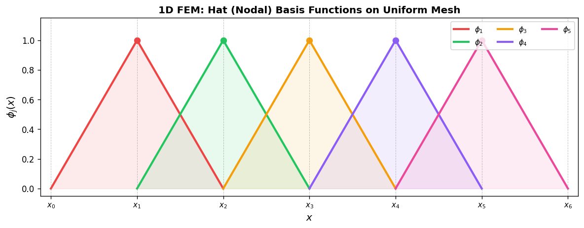
\[ V_h^k = \left\{ u \in C^0 : u\big|_{K_j} \in P^k(K_j)\; \forall K_j,\; u(0) = 0 \right\}, \]

where \(P^k(K)\) is the space of polynomials of degree \(k\) on element \(K\). For \(k = 1\) we use the hat (nodal) basis: \(\phi_j(x_i) = \delta_{ij}\) (Kronecker delta), giving piecewise linear functions

\[ \phi_j(x) = \begin{cases} (x - x_{j-1})/(x_j - x_{j-1}), & x_{j-1} \le x \le x_j, \\ (x_{j+1} - x)/(x_{j+1} - x_j), & x_j \le x \le x_{j+1}, \\ 0, & \text{otherwise.} \end{cases} \]

Each global basis function is nonzero only on the two elements sharing node \(x_j\). We also introduce local (element) basis functions on \(K_k = [x_{k-1}, x_k]\):

\[ \psi_{k,1}(x) = \frac{x_k - x}{x_k - x_{k-1}}, \qquad \psi_{k,2}(x) = \frac{x - x_{k-1}}{x_k - x_{k-1}}, \]

so \(\psi_{k,1} = \phi_{k-1}\) and \(\psi_{k,2} = \phi_k\) on \(K_k\). The key feature of these basis functions is their compact support — they are nonzero only on a small number of elements, leading to a sparse stiffness matrix.

2.2.3 Imposing the Dirichlet Boundary Condition

We set \(G = \alpha\phi_0(x) = \alpha\psi_{1,1}(x)\), where \(\phi_0(x_0) = 1\) and \(\phi_0(x_i) = 0\) for \(i = 1, \ldots, N\). This satisfies the Dirichlet condition exactly.

2.2.4 Element Matrices and Assembly

We introduce element stiffness matrices and element load vectors for each element \(K_k\):

\[ A^{(k)}_{ij} = \int_{K_k} \kappa(x)\frac{d\psi_{k,j}}{dx}\frac{d\psi_{k,i}}{dx}\,dx, \qquad F^{(k)}_i = \int_{K_k} f(x)\psi_{k,i}\,dx. \]

The global system is assembled by summing element contributions according to the local-to-global node mapping. For interior nodes \(k = 2, \ldots, N-1\), the assembly yields

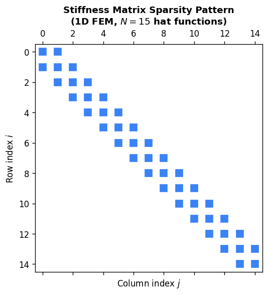
\[ A^{(k)}_{21} U_{k-1} + \left(A^{(k)}_{22} + A^{(k+1)}_{11}\right) U_k + A^{(k+1)}_{12} U_{k+1} = F^{(k)}_2 + F^{(k+1)}_1. \]

The assembled global matrix \(A\) is symmetric positive definite and banded (tridiagonal for linear elements), making it computationally efficient to solve.

2.2.5 Mapping to the Reference Element

To compute element integrals efficiently, we introduce the reference element \(\hat{K} = [0,1]\) and the affine mapping

\[ F_{K_j}: (0,1) \to (x_{j-1}, x_j): \xi \mapsto x = h_j\xi + x_{j-1}. \]

The reference basis functions are \(\hat{\psi}_1(\xi) = 1 - \xi\) and \(\hat{\psi}_2(\xi) = \xi\).

The element integrals transform to \[ A^{(k)}_{ij} = \frac{1}{h_k}\int_0^1 \kappa(x(\xi))\frac{d\hat{\psi}_j}{d\xi}\frac{d\hat{\psi}_i}{d\xi}\,d\xi, \qquad F^{(k)}_i = \int_0^1 f(x(\xi))\hat{\psi}_i(\xi)h_k\,d\xi. \]

When exact integration is not possible, we use Gaussian quadrature on \([0,1]\):

\[ \int_0^1 g(\xi)\,d\xi \approx \sum_{i=1}^n \tfrac{1}{2}b_i\,g\!\left(\tfrac{1}{2}c_i + \tfrac{1}{2}\right). \]

For 3-point Gaussian quadrature (\(n = 3\), the weights and nodes are \(b_1 = 8/9, c_1 = 0\); \(b_2 = b_3 = 5/9\), \(c_{2,3} = \mp\sqrt{3/5}\).

2.3 Example: Constant-Coefficient Poisson Problem

Example 2.3. Consider the BVP \(-d^2u/dx^2 = f\) on \((0,1)\) with \(u(0) = \alpha\) and \(-du/dx = \beta\) at \(x = 1\), where \(f, \alpha, \beta\) are constants and we use a uniform mesh \(h_j = h = 1/N\).

The element matrices and vectors are

\[ A^{(k)}_{ij} = \frac{1}{h}\begin{cases} 1 & \text{if } ij = 11 \text{ or } 22, \\ -1 & \text{if } ij = 12 \text{ or } 21, \end{cases} \qquad F^{(k)}_i = \tfrac{1}{2}fh. \]

Assembling the global system gives the tridiagonal system \(\frac{1}{h}\operatorname{tridiag}(-1, 2, -1)\,U = F\), with boundary modifications. Remarkably, this is exactly the same linear system produced by the standard second-order finite difference method applied to the same problem (with a ghost point for the Neumann condition). However, the finite element method generalises far more easily to non-uniform grids, non-constant coefficients, and higher dimensions.

---

Section 3: Time-Dependent PDEs — The Heat Equation

(Lecture 11)

Many problems in science involve time-dependent PDEs. We discuss the CG finite element method for the parabolic heat equation: given forcing \(f(x,t)\) and initial condition \(g(x)\), seek \(u\) such that

\[ \partial_t u - \partial_{xx} u = f \quad \text{for } x \in (0,1),\; t > 0, \]

with \(u(0,t) = u(1,t) = 0\) and \(u(x,0) = g(x)\).

3.1 Weak Formulation via Time Discretization

We adopt the method of lines approach: discretize in time first, then in space. Using a uniform time step \(\Delta t\), the Backward Euler scheme approximates \(\partial_t u \approx (u^{n+1} - u^n)/\Delta t\). Setting \(\tau = \Delta t^{-1}\), the semi-discrete problem at each time step is: find \(u^{n+1}\) such that

\[ \tau u^{n+1} - \frac{d^2}{dx^2}u^{n+1} = f^{n+1} + \tau u^n \quad \text{in } \Omega. \]

Multiplying by a test function \(v \in V = \{v \in L^2(0,1) : v' \in L^2(0,1),\; v(0) = v(1) = 0\}\) and integrating:

\[ \tau\int_0^1 u^{n+1}v\,dx + \int_0^1 \frac{du^{n+1}}{dx}\frac{dv}{dx}\,dx = \int_0^1 (f^{n+1} + \tau u^n)v\,dx \quad \forall v \in V. \]

This has the same structure as the elliptic weak formulation in Section 2, with the addition of a mass term \(\tau \int u^{n+1} v\) on the left.

3.2 Matrix Form

With the same nodal basis \(\{\phi_1, \ldots, \phi_{N-1}\}\) (no \(\phi_N\) since both endpoints are Dirichlet), the discrete problem is

\[ AU^{n+1} = F^{n+1}, \quad A \in \mathbb{R}^{(N-1)\times(N-1)}, \]

where

\[ a_{ij} = \int_0^1 \left(\tau \phi_j\phi_i + \frac{d\phi_j}{dx}\frac{d\phi_i}{dx}\right)dx, \qquad F_i^{n+1} = \int_0^1 (f^{n+1} + \tau u_h^n)\phi_i\,dx. \]

The stiffness matrix \(A\) now includes both stiffness and mass contributions; crucially, it does not change between time steps, so it need only be assembled and factored once. Only the right-hand side \(F^{n+1}\) changes at each step. The solution advances as \(U^{n+1} = A^{-1}F^{n+1}\).

---

Section 4: Well-Posedness and Error Analysis

(Lectures 11–22)

Lectures 11–22 develop the mathematical analysis of the finite element method. The key results, drawn from Chapters 1, 2, and 5 of Brenner–Scott, include:

• Existence and uniqueness of weak solutions via the Lax–Milgram theorem: if \(a(\cdot, \cdot)\) is continuous and coercive and \(\ell(\cdot)\) is continuous, a unique weak solution exists.
• Galerkin orthogonality: \(a(u - u_h, v_h) = 0\) for all \(v_h \in V_h\) — the error is orthogonal (in the energy inner product) to the discrete space.
• Céa’s lemma: the FEM error is quasi-optimal: \(\|u - u_h\|_V \le C \inf_{v_h \in V_h}\|u - v_h\|_V\).
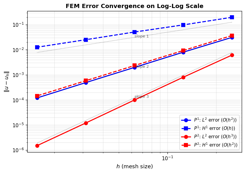
• Interpolation estimates: for smooth \(u\) and piecewise linear elements, \(\|u - u_h\|_{L^2} = O(h^2)\) and \(\|u - u_h\|_{H^1} = O(h)\).
• H¹ and L² error estimates via the Aubin–Nitsche duality argument.

---

Section 5: Implementing the CG Finite Element Method in 2D

(Lectures 23–25)

5.1 The 2D Poisson Problem and Weak Formulation

We extend the FEM to two dimensions. Consider the Poisson problem: let \(\Omega \subset \mathbb{R}^2\) be a polygonal domain with boundary \(\partial\Omega\). Given \(f: \Omega \to \mathbb{R}\) and Dirichlet data \(g_D: \partial\Omega \to \mathbb{R}\), find \(u: \Omega \to \mathbb{R}\) such that

\[ -\Delta u = f \quad \text{in } \Omega, \qquad u = g_D \quad \text{on } \partial\Omega. \]

The Poisson problem models temperature distributions, gravitational and electromagnetic potentials, and inviscid flow. As in 1D, non-smooth data may prevent the existence of a classical solution.

Example 5.1. Take \(\Omega = (-1,1)^2\) and let \(f = 1\) on \(\{x > 0\}\) and \(f = 0\) on \(\{x < 0\}\). Since \(f\) is discontinuous, the solution satisfies \(u \notin C^2(\Omega)\) and no classical solution exists.

To derive the weak formulation, multiply \(-\Delta u = f\) by a smooth test function \(v\) with \(v|_{\partial\Omega} = 0\) and integrate. By Green’s identity:

\[ \int_\Omega \nabla u \cdot \nabla v\,dx = \int_\Omega vf\,dx. \]

Define the Sobolev space

\[ H^1(\Omega) := \left\{ u: \Omega \to \mathbb{R} \;\middle|\; u,\, \tfrac{\partial u}{\partial x},\, \tfrac{\partial u}{\partial y} \in L^2(\Omega) \right\}, \]

and the trial and test spaces

\[ H^1_g(\Omega) := \{ u \in H^1(\Omega) : u|_{\partial\Omega} = g_D \}, \qquad H^1_0(\Omega) := \{ v \in H^1(\Omega) : v|_{\partial\Omega} = 0 \}. \]

Definition 5.4 (Weak formulation). Let \(f \in L^2(\Omega)\). Find \(u \in H^1_g(\Omega)\) such that

\[ \int_\Omega \nabla u \cdot \nabla v\,dx = \int_\Omega vf\,dx \quad \forall v \in H^1_0(\Omega). \]

Unlike the 1D case, the trial function \(u\) and test function \(v\) belong to different spaces (a purely technical simplification for implementation).

5.2 Approximation of the Weak Formulation

Let \(V_{0h} \subset H^1_0(\Omega)\) be an \(N\)-dimensional space with basis \(\{\phi_1, \ldots, \phi_N\}\). To enforce the Dirichlet condition, extend the basis by \(\phi_{N+1}, \ldots, \phi_{N+N_\partial}\) so that \(\sum_{j=N+1}^{N+N_\partial} U_j \phi_j\) interpolates \(g_D\) on \(\partial\Omega\). The finite element solution is

\[ u_h = \sum_{j=1}^N U_j\phi_j + \sum_{j=N+1}^{N+N_\partial} U_j\phi_j. \]

Definition 5.5 (FEM weak formulation). Let \(f \in L^2(\Omega)\). Find \(u_h \in V_{gh}\) such that

\[ \int_\Omega \nabla u_h \cdot \nabla v_h\,dx = \int_\Omega v_h f\,dx \quad \forall v_h \in V_{0h}. \]

This yields the global linear system \(AU = F\) with

\[ a_{ij} = \int_\Omega \nabla\phi_j \cdot \nabla\phi_i\,dx, \qquad F_i = \int_\Omega \phi_i f\,dx - \sum_{j=N+1}^{N+N_\partial} U_j \int_\Omega \nabla\phi_j \cdot \nabla\phi_i\,dx. \]

5.3 Discretization on Unstructured Triangular Meshes

A key advantage of finite elements is their ability to handle unstructured grids on complex geometries. We discretize \(\Omega\) with a triangulation \mathcal{T}_h) of triangles \(K_k\) satisfying: \(\cup_k \overline{K_k} = \Omega\), triangles do not overlap, and vertices of neighboring triangles coincide.

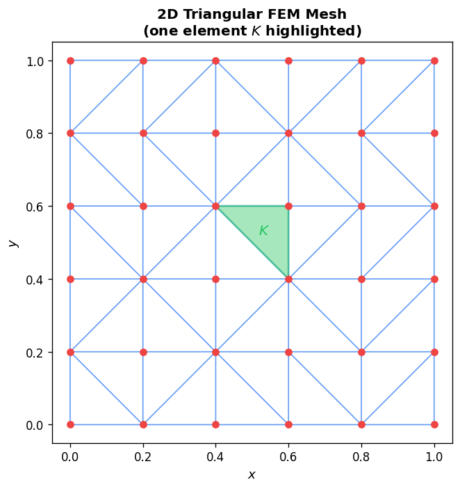
Local basis functions. Each triangle \(K_k\) has three local degrees of freedom (one per vertex) with basis set \(\Sigma_k = \{\psi_{k,1}, \psi_{k,2}, \psi_{k,3}\}\). The local solution in element \(K_k\) is

\[ u_h|_{K_k} = \sum_{i=1}^3 U_i^{(k)}\psi_{k,i}. \]

5.3.1 Computing Element Matrices via the Reference Triangle

We introduce the reference triangle \(\hat{K}\) with local coordinates \((\xi, \eta)\) and the affine mapping

\[ F_{K_k}: \hat{K} \to K_k: \boldsymbol{\xi} \mapsto \mathbf{x} = \mathbf{q}_1\hat{\psi}_1 + \mathbf{q}_2\hat{\psi}_2 + \mathbf{q}_3\hat{\psi}_3 = \mathbf{q}_1 + J_k\boldsymbol{\xi}, \]

where \(\mathbf{q}_i = (x_i, y_i)\) are the physical vertices and the Jacobian matrix is

\[ J_k = \begin{pmatrix} x_2 - x_1 & x_3 - x_1 \\ y_2 - y_1 & y_3 - y_1 \end{pmatrix}, \qquad \det(J_k) = \pm 2|K_k|, \]

where \(|K_k|\) is the area of triangle \(K_k\). The reference basis functions are

\[ \hat{\psi}_1 = 1 - \xi - \eta, \quad \hat{\psi}_2 = \xi, \quad \hat{\psi}_3 = \eta. \]

The physical gradients relate to reference gradients by the chain rule:

\[ \nabla\psi_{k,i}(\mathbf{x}) = J_k^{-T}\hat{\nabla}\hat{\psi}_i(\boldsymbol{\xi}), \qquad J_k^{-T} = \frac{1}{\det(J_k)}\begin{pmatrix} y_3 - y_1 & y_1 - y_2 \\ x_1 - x_3 & x_2 - x_1 \end{pmatrix}. \]

The reference gradients of the linear basis functions are constant:

\[ \hat{\nabla}\hat{\psi}_1 = \begin{pmatrix}-1\\-1\end{pmatrix}, \quad \hat{\nabla}\hat{\psi}_2 = \begin{pmatrix}1\\0\end{pmatrix}, \quad \hat{\nabla}\hat{\psi}_3 = \begin{pmatrix}0\\1\end{pmatrix}. \]

Since these gradients are constant, the element stiffness matrix is exact (no quadrature needed for linear elements):

\[ A^{(k)}_{ij} = \int_{K_k}\nabla\psi_{k,i}\cdot\nabla\psi_{k,j}\,dx = \tfrac{1}{2}\det(J_k)\left(J_k^{-T}\hat{\nabla}\hat{\psi}_i\right)\cdot\left(J_k^{-T}\hat{\nabla}\hat{\psi}_j\right). \]

For the load vector with constant \(f\), integrating over the reference triangle:

\[ F^{(k)}_i = f\det(J_k)\int_0^1\int_0^{1-\xi}\hat{\psi}_i\,d\eta\,d\xi, \]

which gives \(F^{(k)}_1 = F^{(k)}_2 = F^{(k)}_3 = \frac{1}{3}f|K_k|\). For non-constant \(f\), use 7-point Gaussian quadrature on the reference triangle, which is exact for polynomials of degree up to 4.

5.3.2 Global Assembly and Dirichlet Boundary Conditions

Assembly uses the connectivity matrix \(P\): entry \(P(k,i)\) gives the global node number of local node \(i\) in element \(k\). The global system is assembled as:

for k = 1:NumElements
  for j = 1:3
    for i = 1:3
      A_global(P(k,i), P(k,j)) += A(k,i,j)
    end
    F_global(P(k,j)) += F(k,j)
  end
end

Dirichlet boundary conditions are imposed by row elimination: for each boundary node \(r\), set \(A_{rr} = 1\), zero all other entries in row \(r\), and set \(F_r = g_D(x_r)\).

---

Section 6: The Finite Volume and Discontinuous Galerkin Methods for Scalar Hyperbolic Conservation Laws in 1D

(Lectures 26–34)

6.0 Method of Characteristics

Before developing numerical methods for hyperbolic conservation laws, it is essential to understand how solutions propagate. For the linear advection equation \(u_t + au_x = 0\) on \(-\infty < x < \infty\), consider the behaviour of \(u\) restricted to a curve \(x(t)\) in the \(x\)–\(t\) plane. Differentiating along the curve,

\[ \frac{d}{dt}u(x(t), t) = u_x\frac{dx}{dt} + u_t = u_x\frac{dx}{dt} - au_x = \left(\frac{dx}{dt} - a\right)u_x. \]

If we choose the curve so that \(dx/dt = a\), then \(d/dt\,[u(x(t),t)] = 0\): the solution is constant along the curve. These special curves are called characteristics; for the linear advection equation they are the straight lines \(x(t) = at + x_0\). Given initial data \(u(x,0) = u_0(x)\), we trace back along the characteristic through \((x,t)\) to the \(t=0\) axis: the foot of the characteristic is \(x_0 = x - at\), and the solution is

\[ u(x,t) = u_0(x - at). \]

The initial profile simply translates to the right (if \(a > 0\)) at speed \(a\) without changing shape. This tells us two things about proper numerical schemes: they should preserve solution magnitude (no artificial damping or amplification), and they should distinguish the direction of propagation — the “upwind” direction.

For the nonlinear Burgers’ equation \(u_t + uu_x = 0\), the method of characteristics still applies. Along a curve satisfying \(dx/dt = u\), the solution is constant: \(u(x(t),t) = u_0(x_0)\). But now the characteristic speed equals the solution value, so characteristics emanating from different points travel at different speeds. When a faster characteristic overtakes a slower one, characteristics cross — the solution becomes multi-valued, and a shock (discontinuity) must form.

Consider the Riemann initial condition \(u_0(x) = 0\) for \(x < 0\) and \(u_0(x) = 1\) for \(x \ge 0\). The characteristics from the left travel at speed 0 (staying vertical in the \(x\)–\(t\) plane), while those from the right travel at speed 1. Moving left to right, the speed jumps from 1 to 0 — characteristics converge. Contrast this with the reversed Riemann problem \(u_0(x) = 1\) for \(x < 0\) and \(u_0(x) = 0\) for \(x \ge 0\): characteristics diverge, leaving a wedge-shaped region of the \(x\)–\(t\) plane uncovered. The correct solution for this rarefaction (expansion) wave is the fan-shaped function \(u(x,t) = x/t\) for \(0 < x/t < 1\), interpolating continuously between the two constant states. The domain-of-dependence theorem states that for consistency of any numerical scheme, the exact domain of dependence must lie inside the numerical domain of dependence, recovering the CFL condition \(\Delta x/\Delta t \le |\lambda_{\max}|\).

6.1 The Scalar Hyperbolic Conservation Law

Let \(\Omega = (0,1)\) and \(I = (0,T]\). Given initial condition \(u_0: \Omega \to \mathbb{R}\), we seek \(u: \Omega \times I \to \mathbb{R}\) satisfying

\[ \partial_t u + \partial_x f(u) = 0 \quad \text{in } \Omega \times I, \qquad u(x,0) = u_0(x) \quad \text{in } \Omega, \]

with suitable boundary conditions. The eigenvalue of the scalar conservation law is \(\lambda = \partial f/\partial u\), which plays a central role in numerical methods.

In integral form, integrating over any subinterval \([a,b]\):

\[ \frac{d}{dt}\int_a^b u(x,t)\,dx = f(u(a,t)) - f(u(b,t)). \]

This expresses the conservation principle: the rate of change of \(u\) in \([a,b]\) equals the net flux in at \(a\) minus the flux out at \(b\).

Prototypical examples:

• Linear advection: \(f(u) = au\), \(a = \text{const}\), \(\lambda = a\).
• Burgers’ equation: \(f(u) = \tfrac{1}{2}u^2\), \(\lambda = u\) (nonlinear; can develop shocks).

The finite dimensional space for FV and DG methods allows discontinuities at element boundaries:

\[ V_h^d := \left\{ v_h \in L^2(\Omega) : v_h|_{K_j} \in P^k(K_j)\; \forall K_j \right\}. \]

This differs crucially from the CG space (Section 2), which required continuity across elements.

6.1.1 Weak Formulation for FV/DG

Multiplying the conservation law by a smooth test function \(v\) and integrating over element \(K_j = [x_{j-1}, x_j]\) and integrating by parts:

\[ \int_{K_j} v\,\partial_t u\,dx - \int_{K_j} f(u)\,\partial_x v\,dx + f(u(x_j,t))v(x_j) - f(u(x_{j-1},t))v(x_{j-1}) = 0. \]

Replacing smooth functions by discrete ones in \(V_h^d\), we encounter the problem that \(u_h\) is discontinuous at nodes \(x_j\): the left-limit \(u_h^j(x_j)\) and right-limit \(u_h^{j+1}(x_j)\) differ. The flux is therefore undefined at node \(x_j\).

The solution is to replace the exact flux by a numerical flux \(\hat{f}^j = \hat{f}(u_h^j(x_j), u_h^{j+1}(x_j))\). The unified FV/DG method becomes, for each element \(K_j\) and all \(v_h \in V_h^d\):

\[ \int_{K_j} v_h^j\,\partial_t u_h^j\,dx - \int_{K_j} f(u_h^j)\,\partial_x v_h^j\,dx + \hat{f}^j v_h^j(x_j) - \hat{f}^{j-1}v_h^j(x_{j-1}) = 0. \]

Definition 6.2 (Consistent numerical flux). A numerical flux \(\hat{f}(a,b)\) is consistent if \(\hat{f}(u,u) = f(u)\) for all smooth \(u\).

The FV and DG methods coincide up to this point and diverge only in the choice of polynomial degree \(k\) in \(V_h^d\).

6.2 The Finite Volume Method

Setting \(k = 0\) (piecewise constant approximation), the expansion coefficient \(\hat{u}_1^j(t)\) approximates the mean of \(u\) in element \(K_j\):

\[ \hat{u}_1^j(t) \approx \frac{1}{h_j}\int_{K_j} u(x,t)\,dx. \]

With forward Euler time stepping and uniform mesh \(h\) and time step \(\Delta t\), the finite volume scheme is

\[ (\hat{u}_1^j)^n = (\hat{u}_1^j)^{n-1} + \frac{\Delta t}{h}\left(\hat{f}^{n-1}_{j-1} - \hat{f}^{n-1}_j\right), \quad j = 1, \ldots, N,\; n = 1, \ldots, M. \]

This is precisely an approximation to the second integral form of the conservation law. The initial condition is \(\hat{u}_1^j(0) = \frac{1}{h_j}\int_{K_j} u_0(x)\,dx\).

For stability, an explicit time stepping scheme requires the Courant–Friedrichs–Lewy (CFL) condition:

\[ \frac{\Delta t}{h}\,\lambda\!\left((\hat{u}_1^j)^{n-1}\right) \le c \quad \forall j, \quad c \le 1. \]

6.2.1 Discontinuous Solutions and Shocks

A key feature of nonlinear hyperbolic conservation laws is that discontinuities (shocks) can develop from smooth initial conditions. Burgers’ equation with a smooth initial condition can form a shock in finite time as characteristics converge.

Example 6.3. Burgers’ equation \(\partial_t u + \partial_x(\frac{1}{2}u^2) = 0\) with \(u(x,0) = \frac{1}{4} + \frac{1}{2}\sin(\pi x)\) on \((-1,1)\) with periodic boundary conditions develops a shock at approximately \(t = 0.5\).

When a shock at \(x = x_d(t)\) propagates with speed \(S = dx_d/dt\), applying the Leibniz rule to the integral conservation law and taking limits gives the Rankine–Hugoniot condition:

\[ S = \frac{f(u(x_L,t)) - f(u(x_R,t))}{u(x_L,t) - u(x_R,t)}, \]

where \(u(x_L,t)\) and \(u(x_R,t)\) are the left and right limits at the shock. This condition is essential for correctly simulating shock propagation.

Example 6.4 illustrates that manipulating the conservation law (e.g., rewriting Burgers’ in terms of \(u^2\) rather than \(u\) yields a different weak solution. Only the original conservation form gives the physically correct shock speed.

6.2.2 Non-Uniqueness and the Entropy Solution

Example 6.5 shows that an infinite family of weak solutions can exist for the same initial data. Only one is physically relevant: the entropy solution, defined as the unique weak solution satisfying the second law of thermodynamics (entropy must be non-decreasing).

6.2.3 Conservative and Monotone Schemes

Definition 6.7 (Conservative scheme). A scheme of the form

\[ u_j^n = u_j^{n-1} + \frac{\Delta t}{h}\left(\hat{f}_{j-1}^{n-1} - \hat{f}_j^{n-1}\right) \]

is conservative. The FV method (6.18) is conservative. Conservative schemes ensure that their convergent subsequences converge to weak solutions of the conservation law.

Theorem 6.8 (Lax–Wendroff). A conservative scheme, if convergent, converges to a weak solution of the conservation law.

However, this does not guarantee convergence to the entropy solution. For this, we additionally require monotonicity.

Definition 6.9 (Monotone scheme). A scheme is monotone if: when the initial data satisfies \(v_i^{n-1} \ge u_i^{n-1}\) for all \(i\), then \(v_i^n \ge u_i^n\) for all \(i\). Equivalently, the numerical flux must be non-decreasing in its first argument and non-increasing in its second argument.

Theorem 6.10. For a monotone scheme, \(\max_i u_i^n \le \max_i u_i^{n-1}\) and \(\min_i u_i^n \ge \min_i u_i^{n-1}\). This means no new extrema are created — spurious oscillations cannot appear.

Theorem 6.11. A consistent monotone scheme with \(\Delta t/h\) fixed converges to the entropy solution as \(\Delta t \to 0\).

Theorem 6.12 (Godunov’s theorem). A monotone method is at most first order accurate.

This fundamental limitation means that monotone (first-order) FV methods suffer from excessive numerical diffusion (“smearing”), motivating the development of higher-order DG methods.

6.2.4 The Local Lax–Friedrichs Numerical Flux

The local Lax–Friedrichs (LLF) flux (also known as Rusanov’s flux) is:

\[ \hat{f}(a,b) = \tfrac{1}{2}(f(a) + f(b)) - \tfrac{1}{2}\beta(b - a), \]

where \(\beta = \max_{\min(a,b) \le s \le \max(a,b)} |\lambda(s)|\) and \(\lambda(s) = f'(s)\). This flux is consistent, non-decreasing in its first argument, and non-increasing in its second argument — satisfying all monotonicity requirements.

Warning (Example 6.13). The central flux \(\hat{f}(a,b) = \frac{1}{2}(f(a)+f(b))\) must never be used: while consistent, it lacks the required monotonicity properties and leads to instabilities.

Boundary conditions for hyperbolic PDEs are imposed through the numerical flux. A Dirichlet condition \(u(0,t) = u_b(t)\) enters element \(j=1\) via \(\hat{f}(u_b^{n-1}, (\hat{u}_1^1)^{n-1})\).

Example 6.14 (Linear advection). For \(f(u) = \alpha u\), the LLF flux reduces to the upwind scheme: if \(\alpha > 0\), use the value from the left; if \(\alpha < 0\), use the value from the right. The CFL condition is \(\Delta t \le ch/|\alpha|\).

Example 6.15 (Burgers’ equation). For \(f(u) = \frac{1}{2}u^2\), \(\beta = \max_{\min(a,b) \le s \le \max(a,b)} |s|\). The CFL condition is \(\Delta t \le ch/\gamma\) where \(\gamma = \max_j |(\hat{u}_1^j)^{n-1}|\).

6.3 The Discontinuous Galerkin Method, k = 1

Setting \(k = 1\) (piecewise linear approximation), in each element \(K_j\):

\[ u_h(x,t)|_{K_j} = \hat{u}_1^j(t)\psi_1(x) + \hat{u}_2^j(t)\psi_2(x), \]

where \(\hat{u}_1^j\) is the local mean and \(\hat{u}_2^j\) captures the slope. We use the reference element \(\hat{K} = [-1,1]\) (not \([0,1]\) as in the CG case) with the mapping

\[ F_{K_j}: (-1,1) \to (x_{j-1}, x_j): \xi \mapsto x = \tfrac{1}{2}(x_{j-1} + x_j) + \tfrac{1}{2}h\xi. \]

Legendre basis functions: \(\hat{\psi}_1(\xi) = 1\) and \(\hat{\psi}_2(\xi) = \xi\). The first two Legendre polynomials are chosen because they are orthogonal on \((-1,1)\):

\[ \int_{-1}^1 \hat{\psi}_i(\xi)\hat{\psi}_j(\xi)\,d\xi = \frac{2}{2(i-1)+1}\delta_{ij}. \]

This orthogonality property dramatically simplifies the algebra: the mass matrix on the reference element is diagonal, and many integrals vanish.

Substituting into the weak formulation and using orthogonality, the DG method simplifies to:

\[ \frac{d}{dt}\hat{u}_1^j(t) = \frac{1}{h}\left[\hat{f}^{j-1} - \hat{f}^j\right], \qquad \frac{d}{dt}\hat{u}_2^j(t) = \frac{3}{h}\left[\int_{-1}^1 f(u_h^j(x(\xi),t))\,d\xi - \hat{f}^j + \hat{f}^{j-1}\right]. \]

Remark 6.17. Setting \(\hat{u}_2^j = 0\) in the DG method recovers exactly the finite volume method. The DG solution with \(k=1\) decomposes as: mean value (FV part) plus higher-order slope information.

Initial condition by projecting \(u_0\):

\[ \hat{u}_1^j(0) = \frac{1}{2}\int_{-1}^1 u_0(x(\xi))\,d\xi, \qquad \hat{u}_2^j(0) = \frac{3}{2}\int_{-1}^1 \xi\,u_0(x(\xi))\,d\xi. \]

The integrals may be approximated by 2-point Gaussian quadrature:

\[ \int_{-1}^1 g(\xi)\,d\xi \approx g\!\left(-\tfrac{1}{\sqrt{3}}\right) + g\!\left(\tfrac{1}{\sqrt{3}}\right). \]

6.3.1 Fully Discrete RKDG Formulation

Since the DG method has \(k=1\) and is second-order in space, we need a second-order time stepping scheme of matching accuracy. We use the 2-stage TVD Runge–Kutta method:

\[ \xi^1 = \hat{u}^{n-1} + \Delta t\,L(\hat{u}^{n-1}), \qquad \hat{u}^n = \xi^2 = \tfrac{1}{2}\hat{u}^{n-1} + \tfrac{1}{2}\xi^1 + \tfrac{1}{2}\Delta t\,L(\xi^1), \]

where \(L(\hat{u})\) is the spatial operator. The CFL condition for the DG method with \(k=1\) requires \(c \le 0.3\) (much smaller than the FV requirement of \(c \le 1\).

The method combining DG spatial discretization with TVD-RK time stepping is called the Runge–Kutta Discontinuous Galerkin (RKDG) method.

6.3.2 Convergence and Slope Limiters

By Godunov’s theorem, the second-order DG method cannot be monotone. Without additional treatment, it can produce non-physical oscillations (overshoots and undershoots) near discontinuities, violating conservation.

To address this, define the total variation of the means:

\[ TV((\hat{u}_1)^n) = \sum_{1 \le j \le N-1} |(\hat{u}_1^{j+1})^n - (\hat{u}_1^j)^n|. \]

Definition 6.20 (TVDM). A method is total variation diminishing in the means if \(TV((\hat{u}_1)^n) \le TV((\hat{u}_1)^{n-1})\).

Example 6.21 demonstrates that the RKDG method without slope limiting is not TVDM on Burgers’ equation: the total variation in the means grows in time and oscillations appear.

To enforce TVDM, we apply the minmod slope limiter after each Runge–Kutta stage. The minmod function is:

\[ m(a_1, a_2, a_3) = \begin{cases} s\min(|a_1|, |a_2|, |a_3|) & \text{if } s = \operatorname{sgn}(a_1) = \operatorname{sgn}(a_2) = \operatorname{sgn}(a_3), \\ 0 & \text{otherwise.} \end{cases} \]

Applying the limiter, in each element we replace \(u_h|_{K_j} = \hat{u}_1^j + \hat{u}_2^j\psi_2(x)\) by

\[ \tilde{u}_h|_{K_j} = \hat{u}_1^j + m\!\left(\hat{u}_2^j,\; \hat{u}_1^{j+1} - \hat{u}_1^j,\; \hat{u}_1^j - \hat{u}_1^{j-1}\right)\psi_2(x). \]

The mean \(\hat{u}_1^j\) is preserved (conservation property); only the slope \(\hat{u}_2^j\) is modified. The limiter prevents over- and undershoots by comparing the local slope to differences of neighboring means.

Theorem 6.23 (TVDM property of RKDG with minmod). Under the CFL condition and with nonneg-ative RK coefficients summing to 1, the RKDG method with minmod slope limiting satisfies \(TV((\hat{u}_1)^n) \le TV((\hat{u}_1)^0)\) for all \(n \ge 0\).

Example 6.22 confirms that with the slope limiter, oscillations vanish and the TVDM property is restored.

Example 6.26 compares FV, RKDG without limiter, and RKDG with limiter on the advection equation with a step function initial condition. At \(t = 10\), the FV solution has diffused completely; the RKDG with limiter remains sharp and accurate.

6.4 The Discontinuous Galerkin Method, k > 1

For higher-order accuracy, set \(k = m\). In each element:

\[ u_h(x,t)|_{K_j} = \sum_{i=1}^{m+1} \hat{u}_i^j(t)\psi_i(x), \]

using the first \(m+1\) Legendre polynomials on \(\hat{K} = [-1,1]\):

\[ \hat{\psi}_1 = 1,\quad \hat{\psi}_2 = \xi,\quad \hat{\psi}_3 = \tfrac{1}{2}(3\xi^2 - 1),\quad \hat{\psi}_4 = \tfrac{1}{2}(5\xi^3 - 3\xi), \ldots \]

The general ODE for expansion coefficients is:

\[ \frac{d}{dt}\hat{u}_i^j(t) = \frac{2(i-1)+1}{h}\left[\int_{-1}^1 f(u_h^j(x(\xi),t))\frac{d\hat{\psi}_i}{d\xi}\,d\xi - \hat{f}^j\hat{\psi}_i(1) + \hat{f}^{j-1}\hat{\psi}_i(-1)\right]. \]

Setting \(m = 0\) recovers the FV method; setting \(m = 1\) recovers the \(k = 1\) DG method.

Remark 6.27. For \(k > 1\), two-point Gaussian quadrature is insufficient; use three-point quadrature (exact to degree 5):

\[ \int_{-1}^1 g(\xi)\,d\xi \approx \tfrac{5}{9}g\!\left(-\sqrt{3/5}\right) + \tfrac{8}{9}g(0) + \tfrac{5}{9}g\!\left(\sqrt{3/5}\right). \]

Remark 6.28. A DG method with \(k = m\) achieves order \(m+1\) in space: \(\|u - u_h\| = O(h^{m+1})\). The time stepping scheme must also be of order \(m+1\). For \(m = 2\), use the 3-stage TVD Runge–Kutta method.

Remark 6.29. For \(k = m > 1\), slope limiting is applied by projecting \(u_h\) into the \(k=1\) space and applying minmod; if the slope limiter does not modify the projection, keep the original high-order solution.

---

Section 7: Systems of Hyperbolic Conservation Laws in 1D

(Lectures 33–34)

7.1 Problem Setup and Weak Formulation

We now consider systems of conservation laws. Let \(U: \Omega \times I \to \mathbb{R}^\ell\) be a vector of \(\ell\) conserved variables with flux \(F(U) \in \mathbb{R}^\ell\):

\[ \partial_t U + \partial_x F(U) = 0 \quad \text{in } \Omega \times I, \qquad U(x,0) = U_0(x). \]

We assume that the Jacobian \(\partial F/\partial U\) has \(\ell\) real eigenvalues and a complete set of linearly independent right eigenvectors — making (7.1) a hyperbolic system. Examples include the Euler equations of gas dynamics and the shallow water equations.

The weak formulation proceeds identically to the scalar case, element by element, now testing against a vector test function \(\mathbf{V}_h\). Since the component form is simply the scalar weak form applied to each component of the system, the DG method for systems at polynomial degree \(k = m\) is:

\[ \frac{d}{dt}\hat{U}_{i,r}^j(t) = \frac{2(i-1)+1}{h}\left[\int_{-1}^1 F_r(U_h^j(x(\xi),t))\frac{d\hat{\psi}_i}{d\xi}\,d\xi - \hat{F}^j_{r}\hat{\psi}_i(1) + \hat{F}^{j-1}_{r}\hat{\psi}_i(-1)\right] \]

for \(r = 1, \ldots, \ell\) and \(i = 1, \ldots, m+1\).

7.2 The Finite Volume Method for Systems

Setting \(m = 0\), the FV method for systems with Euler time stepping is:

\[ (\hat{U}_{1,r}^j)^n = (\hat{U}_{1,r}^j)^{n-1} + \frac{\Delta t}{h}\left[\hat{F}^{n-1}_{j-1,r} - \hat{F}^{n-1}_{j,r}\right]. \]

The CFL condition requires \(\frac{\Delta t}{h}\alpha \le c\), where \(\alpha = \max_{1 \le r \le \ell,\, 1 \le j \le N} |\lambda_r((\hat{U}_1^j)^{n-1})|\) is the maximum eigenvalue magnitude across the domain.

7.3 Numerical Fluxes for Systems

Local Lax–Friedrichs (LLF) Flux

Generalising the scalar LLF flux, for systems the LLF flux for component \(r\) is

\[ \hat{F}_r(U^L, U^R) = \tfrac{1}{2}(F^L_r + F^R_r) - \tfrac{1}{2}\beta^j(U^R_r - U^L_r), \quad 1 \le r \le \ell, \]

where \(\beta^j = \max_{1 \le r \le \ell}(|\lambda_r(U^L)|, |\lambda_r(U^R)|)\) is the largest eigenvalue magnitude.

HLL Flux

For systems, the LLF flux can be overly dissipative. A better alternative is the Harten–Lax–van Leer (HLL) flux, which distinguishes between information travelling left and right.

Define the smallest and largest signal velocities:

\[ S_L^j = \min_{1 \le r \le \ell}\left(\lambda_r(U^L), \lambda_r(U^R)\right), \qquad S_R^j = \max_{1 \le r \le \ell}\left(\lambda_r(U^L), \lambda_r(U^R)\right). \]

The HLL intermediate state is derived by applying the Rankine–Hugoniot condition across both \(S_L^j\) and \(S_R^j\):

\[ U_r^{\text{hll}} = \frac{S_R^j U^R_r - S_L^j U^L_r + F^L_r - F^R_r}{S_R^j - S_L^j}. \]

The intermediate flux is then:

\[ F_r^* = \frac{S_R^j F^L_r - S_L^j F^R_r + S_L^j S_R^j(U^R_r - U^L_r)}{S_R^j - S_L^j}. \]

The HLL numerical flux is:

\[ \hat{F}_r(U^L, U^R) = \begin{cases} F^L_r & \text{if } S_L^j \ge 0, \\ F_r^* & \text{if } S_L^j < 0 < S_R^j, \\ F^R_r & \text{if } S_R^j \le 0. \end{cases} \]

Example 7.1: Euler Equations of Gas Dynamics

The Euler equations are the prototypical system of hyperbolic conservation laws:

\[ U = \begin{pmatrix}\rho \\ \rho v \\ E\end{pmatrix}, \quad F(U) = \begin{pmatrix}\rho v \\ \rho v^2 + p \\ v(E+p)\end{pmatrix}, \]

where \(\rho\) is the density, \(v\) the velocity, \(E = \rho(\frac{1}{2}v^2 + e)\) the total energy, and \(p = (γ-1)\rho e\) the pressure (ideal gas). The eigenvalues are \(\lambda_1 = v - a\), \(\lambda_2 = v\), \(\lambda_3 = v + a\), where \(a = \sqrt{\gamma p/\rho}\) is the speed of sound.

For the LLF flux: \(\beta^j = \max(|v^j - a^j|, |v^{j+1} - a^{j+1}|, |v^j + a^j|, |v^{j+1} + a^{j+1}|)\). For the HLL flux: \(S_L^j = \min(v^j - a^j, v^{j+1} - a^{j+1})\) and \(S_R^j = \max(v^j + a^j, v^{j+1} + a^{j+1})\).

Example 7.2 solves the Euler equations with a Riemann initial condition (left state \((\rho,\rho v, E) = (1.0, 0.75, 2.78125)^T\), right state \((0.125, 0, 0.25)^T\) on 100 elements. The LLF flux produces an excessively smeared solution. The HLL flux provides a significantly sharper approximation, especially for the two shocks in the density profile.

---

Section 8: The FV Method for Systems of Hyperbolic Conservation Laws in 2D

(Lecture 35)

8.1 Problem Setup

We generalise to two spatial dimensions. Let \(\Omega \subset \mathbb{R}^2\). We seek \(U: \Omega \times I \to \mathbb{R}^\ell\) such that

\[ \partial_t U + \nabla \cdot F(U) = 0 \quad \text{in } \Omega \times I, \qquad U(x,y,0) = U_0(x,y), \]

where \(F(U) \in \mathbb{R}^{\ell \times 2}\) is the flux tensor.

Example 8.1 (2D shallow water equations):

\[ U = \begin{pmatrix}h \\ hu \\ hv\end{pmatrix}, \quad F(U) = \begin{pmatrix}hu & hv \\ hu^2 + \tfrac{1}{2}gh^2 & huv \\ huv & hv^2 + \tfrac{1}{2}gh^2\end{pmatrix}, \]

where \(h\) is the water depth, \(u, v\) are velocity components, and \(g\) is gravity. The eigenvalues in direction \(\mathbf{n} = (n_x, n_y)\) are \(\lambda_1 = q - \sqrt{gh}\), \(\lambda_2 = q\), \(\lambda_3 = q + \sqrt{gh}\), where \(q = un_x + vn_y\), confirming hyperbolicity.

8.2 The 2D Finite Volume Method

We discretize \(\Omega\) with \(N\) elements (triangles or quadrilaterals) \(K_j\), using piecewise constant approximations. The FV method follows from integrating the conservation law over element \(K_j\) and using Euler time stepping:

\[ (U_{h,r}^j)^n = (U_{h,r}^j)^{n-1} - \frac{\Delta t}{|K_j|}\int_{\partial K_j}\hat{F}^{n-1}_{j,r} \cdot \mathbf{n}\,ds, \]

where \(\mathbf{n}\) is the outward unit normal on \(\partial K_j\) and \(|K_j|\) is the element area. The CFL condition is \(\frac{\Delta t}{h}\alpha \le c\), where \(\alpha\) is the maximum eigenvalue (in absolute value) of the flux in the normal direction across all element boundaries.

The numerical flux in the normal direction is computed at each element face using the LLF flux in the normal direction:

\[ H_r(U^L, U^R) = \tfrac{1}{2}(F^L_r \cdot \mathbf{n} + F^R_r \cdot \mathbf{n}) - \tfrac{1}{2}\beta^j(U^R_r - U^L_r), \]

where \(\beta^j\) is the largest eigenvalue (in absolute value) on the shared face. Alternatively, the HLL flux may be applied in the normal direction.

Example 8.2 (reference): For a DG discretization of the 2D shallow water equations, see the NGSolve tutorial at https://ngsolve.org/docu/latest/i-tutorials/unit-3.4-simplehyp/shallow2D.html.

---

Summary of Methods and Key Properties

Method	Polynomial Degree	Order of Accuracy	Converges to Entropy Solution?
Finite Volume (FV)	\(k = 0\)	1st order	Yes (monotone, consistent)
DG with \(k=1\) + slope limiter	\(k = 1\)	2nd order	Conjectured (numerical evidence)
DG with \(k=m\) + slope limiter	\(k = m\)	\((m+1)\)th order	Conjectured
CG FEM (elliptic)	\(k \ge 1\)	\(O(h^{k+1})\) in \(L^2\)	N/A (not hyperbolic)

Key Theorems

• Lax–Wendroff: Conservative + convergent ⟹ converges to weak solution.
• Theorem 6.11: Consistent + monotone ⟹ converges to entropy solution.
• Godunov’s theorem: Monotone ⟹ at most 1^st order.
• TVDM theorem: RKDG + minmod under CFL ⟹ total variation of means is non-increasing.

Final Exam Topics

Key topics from the 2019 review (applicable to the 2020 exam preparation):

1. Dirichlet boundary conditions for scalar conservation laws
2. Method of characteristics
3. Discontinuous solutions as weak solutions
4. Hyperbolicity of systems
5. Derivation of the first-order Godunov scheme
6. Exact Riemann solver / numerical flux for given \(f\)
7. Rankine–Hugoniot condition derivation
8. Exact and numerical domain of dependence
9. CFL condition and proof
10. Time step size for nonlinear PDEs
11. Conservation property of conservation laws
12. Von Neumann stability analysis
13. Dissipation and dispersion errors
14. Definitions: monotone and TVD methods
15. Harten’s theorem with proof
16. Weak (Galerkin) formulations (FE and DG)
17. Hat functions
18. Mapping and weak formulations on the computational element (FE and DG)
19. Computation of local mass and stiffness matrices (any order)
20. Assembly of mass and stiffness matrices for FEM with linear basis
21. Higher-order bases: general principles
22. Minmod limiter for DGM
23. Two-dimensional weak forms (DG and FEM)
24. Mapping and weak formulations on triangles
25. Multidimensional quadrature (method of undetermined coefficients)
26. Lagrangian basis functions on triangles

---

References

1. S. C. Brenner and L. R. Scott. The Mathematical Theory of Finite Element Methods. Springer, 3^rd ed., 2008.
2. B. Cockburn. An introduction to the discontinuous Galerkin method for convection-dominated problems. Advanced Numerical Approximation of Nonlinear Hyperbolic Equations, 150–268, 1998.
3. B. Cockburn. Devising discontinuous Galerkin methods for non-linear hyperbolic conservation laws. J. Comput. Appl. Math., 128:187–204, 2001.
4. B. Cockburn and C.-W. Shu. TVB Runge-Kutta local projection discontinuous Galerkin finite element method for conservation laws II. Math. Comp., 52(186):411–435, 1989.
5. B. Cockburn and C.-W. Shu. The Runge-Kutta discontinuous Galerkin method for conservation laws V. J. Comput. Phys., 141(2):199–224, 1998.
6. J. Flaherty. Finite Element Lecture Notes.
7. P. D. Lax and B. Wendroff. Systems of conservation laws. Comm. Pure Appl. Math., 13:217–237, 1960.
8. R. J. LeVeque. Numerical Methods for Conservation Laws. Birkhäuser, 2^nd ed., 1992.
9. R. J. LeVeque. Finite Volume Methods for Hyperbolic Problems. Cambridge Univ. Press, 2002.
10. C.-W. Shu and S. Osher. Efficient implementation of essentially non-oscillatory shock-capturing schemes. J. Comput. Phys., 77(2):439–471, 1988.
11. E. F. Toro. Riemann Solvers and Numerical Methods for Fluid Dynamics. Springer, 3^rd ed., 2009.
12. J. van Kan, A. Segal, and F. Vermolen. Numerical Methods in Scientific Computing. VSSD, 2005.