AMATH 390: Mathematics and Music
K.A. Morris
Estimated study time: 2 hr 19 min
Table of contents
Chapter 1: Harmonic Motion
The second-order differential equation
\[ y'' + \omega^2 y = 0 \tag{1.1} \]sometimes called the oscillator equation, arises in many contexts. For example, for a body with mass \(m\) and an applied force \(F\), Newton’s Second Law implies that the resulting acceleration \(a\) is
\[ ma = F \tag{1.2} \]Letting deflection be \(y\),
\[ my'' = F, \]where \(y''(t)\) is the second derivative of \(y(t)\) with respect to \(t\). For many systems, the restoring force is (approximately) proportional to deflection. For example, in a spring the restoring force is \(-ky\), where \(k\) is known as the spring constant. Letting \(k > 0\) indicate a proportionality constant,
\[ my'' = -ky. \tag{1.3} \]Defining \(\omega = \sqrt{\frac{k}{m}}\), we can rewrite equation (1.3) as (1.1).
The solution to equation (1.1) is, for arbitrary constants \(A\) and \(B\),
\[ y(t) = A\cos(\omega t) + B\sin(\omega t). \tag{1.4} \]This can be verified by direct substitution:
\[ \begin{aligned} y'(t) &= -A\omega\sin(\omega t) + B\omega\cos(\omega t), \\ y''(t) &= -A\omega^2\cos(\omega t) - B\omega^2\sin(\omega t) \\ &= -\omega^2 y(t). \end{aligned} \]In order to fully determine the solution, the initial conditions \(y(0)\) and \(\dot{y}(0)\) are needed. These determine the values of \(A\) and \(B\).
There is another, often more convenient, way to write the solution to (1.1). Using the sum formula
\[ \sin(a + b) = \sin(a)\cos(b) + \cos(a)\sin(b), \tag{1.5} \]leads to writing
\[ y(t) = \beta \cdot \sin(\omega t + \phi), \tag{1.6} \]as
\[ y(t) = \beta\sin(\phi)\cos(\omega t) + \beta\cos(\phi)\sin(\omega t). \tag{1.7} \]Comparing the coefficients of \(\sin(\omega t)\) and \(\cos(\omega t)\) in (1.4) and (1.7) yields
\[ A = \beta\sin(\phi), \quad B = \beta\cos(\phi). \tag{1.8} \]If we define
\[ \beta := \sqrt{A^2 + B^2}, \quad \phi := \arctan\left(\frac{A}{B}\right), \tag{1.9} \]then
\[ y(t) = \beta\sin(\omega t + \phi). \tag{1.10} \]Thus, (1.4) (with \(A\), \(B\) determined by initial conditions) and (1.10) (with \(\beta\), \(\phi\) determined by initial conditions) are equivalent ways of writing the solution to (1.1). This is sometimes called Harmonic Motion.
The advantage of the second representation (1.10) is that it is clear that the solution is periodic with frequency \(\omega\). The amplitude \(\beta\) and phase shift \(\phi\) are determined by initial conditions.
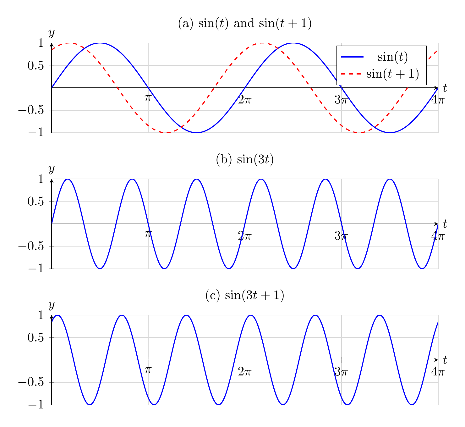
The frequency of the wave corresponds to pitch of an audible sound, while the amplitude of the wave corresponds to loudness. A difference in phase of two waves (an example is shown in Figure 1.1(a)) is not audible. The frequency of \(\sin(\omega t)\) is \(\omega\) rad/s, or \(\frac{\omega}{2\pi}\) Hz.
Differential equations of the form
\[ Ay'' + By' + Cy = 0 \tag{1.11} \](where \(A\), \(B\), \(C\) are constants) are called linear homogeneous second-order ordinary differential equations. Equation (1.1) is an example of this.
For linear differential equations, the Principle of Superposition states that if \(y_1\) and \(y_2\) are both solutions to some linear homogeneous differential equation, then \(y(t) = c_1 y_1(t) + c_2 y_2(t)\) is also a solution to the equation, where \(c_1\) and \(c_2\) are arbitrary constants. This can be verified by substitution. For example, given that \(y_1(t) = \sin(t)\) and \(y_2(t) = \cos(t)\) are both solutions to the differential equation \(y''(t) = -y(t)\), then
\[ y(t) = A\sin(t) + B\cos(t) \tag{1.12} \]is also a solution.
Beats
Consider two waves with the same phase and amplitude, but different frequencies \(\omega_2 > \omega_1\):
\[ y(t) = \sin(\omega_1 t) + \sin(\omega_2 t). \tag{1.13} \]Define
\[ \bar{\omega} = \frac{1}{2}(\omega_2 + \omega_1), \quad \Delta = \frac{1}{2}(\omega_2 - \omega_1), \tag{1.14} \]and use the sum formula (1.5) to write
\[ \begin{aligned} y(t) &= \sin(\bar{\omega}t - \Delta t) + \sin(\bar{\omega}t + \Delta t) \\ &= 2\cos(\Delta t)\sin(\bar{\omega}t). \end{aligned} \]If \(\Delta\) is small, this looks like a sine wave with frequency \(\frac{\bar{\omega}}{2\pi}\) Hz, with a periodic amplitude given by a slow cosine wave. The word beat refers to a periodic fluctuation in the amplitude of a wave. Thus, when two waves of slightly different frequencies are superimposed, beats are produced.
Formally, the frequency of the beats produced by the superposition of two waves \(\sin(\omega_1 t)\) and \(\sin(\omega_2 t)\) is \(\Delta\). However, since it is the amplitude of the envelope that is heard, and this has frequency
\[ \omega_{\text{beats}} = \omega_2 - \omega_1. \tag{1.15} \]This is known as the beat frequency.

Damping
Actual systems do not oscillate forever; there are dissipative forces. A more realistic model of vibration includes a dissipative term proportional to the speed of motion \(y'\), and takes the form
\[ y'' + 2\xi\omega y' + \omega^2 y = 0, \quad 0 < \xi < 1. \tag{1.16} \]Equation (1.16) has solution
\[ \begin{aligned} y(t) &= e^{-\xi\omega t}\left(A\cos\left(\sqrt{1-\xi^2}\,\omega t\right) + B\sin\left(\sqrt{1-\xi^2}\,\omega t\right)\right) \\ &= Ce^{-\xi\omega t}\sin\left(\sqrt{1-\xi^2}\,\omega t + \phi\right) \end{aligned} \]where \(A\), \(B\) (or equivalently \(C\), \(\phi\) are determined by initial conditions. The damped solution has a decaying amplitude, and a slightly lower frequency. With \(\xi = 0.05\), frequency is 99.8% of the undamped frequency. If \(\xi = 0.2\), it’s 98%. Since we are typically concerned only with frequency, and damping only slightly affects frequency, we will not generally include damping in the analysis.

Forced Harmonic Motion
Forced motion occurs when the oscillation of one body forces another body to oscillate. With a forcing term \(f(t)\), the differential equation modelling the motion is
\[ y'' + 2\xi\omega y' + \omega^2 y = f(t), \quad 0 < \xi < 1. \tag{1.17} \]If the forcing is periodic so that \(f(t) = F\sin(\alpha t)\) for some amplitude \(F\) and frequency \(\alpha\), (1.17) becomes
\[ y'' + 2\xi\omega y' + \omega^2 y = F\sin(\alpha t), \quad 0 < \xi < 1, \tag{1.18} \]for some constant \(F\) and frequency \(\alpha\).
The forcing adds a term in the solution of equation (1.18) of the form
\[ y_p(t) = a\sin(\alpha t) + b\cos(\alpha t). \tag{1.19} \]Substituting this into the left-hand-side of (1.18) yields the expressions
\[ \underbrace{(-a\alpha^2 - 2\xi\omega\alpha b + \omega^2 a)}_{F}\sin(\alpha t) + \underbrace{(-b\alpha^2 - 2\xi\omega\alpha a + \omega^2 b)}_{0}\cos(\alpha t). \tag{1.20} \]For this to equal the right-hand-side of (1.18),
\[ \begin{aligned} F &= (\omega^2 - \alpha^2)a + (-2\xi\omega\alpha)b \\ 0 &= (2\xi\omega\alpha)a + (\omega^2 - \alpha^2)b. \end{aligned} \]If \(\alpha \neq \omega\) or \(\xi \neq 0\),
\[ a = \frac{(\omega^2 - \alpha^2)F}{(\omega^2 - \alpha^2)^2 + (2\xi\omega\alpha)^2}, \quad b = \frac{-(2\xi\omega\alpha)F}{(\omega^2 - \alpha^2)^2 + (2\xi\omega\alpha)^2}. \tag{1.21} \]Writing \(\omega_0 = \sqrt{1 - \xi^2}\,\omega\), any solution to (1.18) is of the form
\[ \begin{aligned} y(t) &= e^{-\xi\omega t}(A\sin(\omega_0 t) + B\cos(\omega_0 t)) + a\sin(\alpha t) + b\cos(\alpha t) \\ &= e^{-\xi\omega t}C\sin(\omega_0 t + \phi) + M\sin(\alpha t + \phi_f). \end{aligned} \]where \(M\) and \(\phi_f\) are determined by the forcing function parameters \(F\) and \(\alpha\):
\[ M = \sqrt{a^2 + b^2} = \frac{F}{\sqrt{(\omega^2 - \alpha^2)^2 + (2\xi\omega\alpha)^2}}. \]The constants \(C\) and \(\phi\) (or \(A\) and \(B\) are determined by the initial conditions. Note that as \(t \to \infty\), \(y(t) \to M\sin(\alpha t + \phi_f)\).
The response is the sum of two waves: a decaying wave at the natural frequency \(\omega_0\), and a persistent wave at the forcing frequency \(\alpha\). Thus, in steady-state, once the effect of the initial conditions has dissipated,
\[ y(t) = M\sin(\alpha t + \phi_f), \]where
\[ M = \frac{F}{\sqrt{(\omega^2 - \alpha^2)^2 + (2\xi\omega\alpha)^2}}. \]The value of \(M\) is the magnitude of the steady-state oscillations. The magnitude increases as the forcing frequency \(\alpha\) approaches the natural frequency \(\omega\), and the peak is larger for lightly damped systems. A vibrating system that is forced at a frequency close to the natural frequency is said to be in resonance. There are many instances of resonance; a famous example is a singer breaking a wine glass with their voice, another is Nuclear Magnetic Resonance.

Chapter 2: Stringed Instruments
The sound in many musical instruments, for instance guitars and violins, and also pianos, is produced by vibrating strings. In all these instruments a string is stretched and fixed at each end. The sound is produced by plucking, strumming, or striking the string.
The Dynamics of a Stretched Spring
Consider a string illustrated in Figure 2.2. Let \(u(x,t)\) indicate the deflection from the rest position at position \(x\) along the string and time \(t\). (Set the deflection \(u = 0\) when the string is not stretched by strumming, striking, etc.) Assume constant tension force \(\tau\), density \(\rho\), uniform cross-sectional area \(A\), and small deflections \(u(x,t)\).

Consider a small section of string of length \(\Delta x\). It has mass \(m = \rho A \Delta x\) and acceleration \(a = \frac{\partial^2 u(x,t)}{\partial t^2}\). In this case, the function \(u\) depends on both \(t\) and \(x\). The notation \(\frac{\partial u}{\partial t}\) means take the derivative of \(u\) with respect to \(t\), regarding \(x\) as constant; and similarly for \(\frac{\partial u}{\partial x}\). Assume the only force on the stretched string is tension. The vertical component of the force due to tension is
\[ F = -\tau\sin(\theta(x)) + \tau\sin(\theta(x + \Delta x)). \]Newton’s second law is \(ma = F\), and here
\[ m = \rho A \Delta x, \quad a = \frac{\partial^2 u(x,t)}{\partial t^2}. \]Substitute the expressions for mass (\(m\), acceleration (\(a\), and force \(F\) and dividing through by \(\Delta x\) yields
\[ \rho\frac{\partial^2 u(x,t)}{\partial t^2} = \frac{\tau}{A}\frac{1}{\Delta x}(\sin(\theta(x + \Delta x)) - \sin(\theta(x))). \]Take the limit as \(\Delta x \to 0\) and define \(c^2 = \frac{\tau}{\rho A}\):
\[ \frac{\partial^2 u(x,t)}{\partial t^2} = c^2 \frac{\partial}{\partial x}\sin(\theta(x)). \tag{2.1} \]For small deflections, \(\sin(\theta) \approx \tan(\theta) = \frac{\partial u}{\partial x}\). Equation (2.1) becomes the wave equation
\[ \frac{\partial^2 u}{\partial t^2} = c^2 \frac{\partial^2 u}{\partial x^2}. \tag{2.2} \]The wave equation models vibrations \(u\) in a string, such as a guitar or violin string.
Since the string is fixed at each end, the boundary conditions are
\[ u(0,t) = 0, \quad u(\ell, t) = 0. \tag{2.3} \]Consider initial conditions given by arbitrary functions \(f\) and \(g\):
\[ u(x,0) = f(x), \quad \frac{\partial u}{\partial t}(x,0) = g(x), \tag{2.4} \]where \(f\) and \(g\) describe the initial deflection and velocity respectively of the stretched string.
Solution of the Wave Equation
Partial differential equations are in general very difficult to solve. Try looking for solutions of the form
\[ u(x,t) = M(x)N(t). \]Substitution into (2.2) yields, using \('\) to indicate differentiation,
\[ MN'' = c^2 M'' N. \]Rearranging,
\[ \frac{N''}{c^2 N} = \frac{M''}{M}. \]Since the left-side depends only on time \(t\) and the right-side depends only on space \(x\), each side must be a constant. Call this constant \(-\lambda\). This yields two ordinary differential equations
\[ \begin{align} M''(x) &= -\lambda M(x), \tag{2.7} \\ N'' &= -c^2\lambda N. \tag{2.8} \end{align} \]The boundary conditions also need to be considered: for all time \(t \geq 0\),
\[ M(0)N(t) = 0, \quad M(\ell)N(t) = 0. \]The choice \(N(t) \equiv 0\) yields the trivial solution (which in general does not satisfy the initial conditions), so
\[ M(0) = 0, \quad M(\ell) = 0. \]The spatial function \(M\) should satisfy (2.7) and the boundary conditions. The family of all possible solutions to (2.7) is
\[ M(x) = A\cos(\sqrt{\lambda}\,x) + B\sin(\sqrt{\lambda}\,x). \]From the boundary condition at \(x = 0\), \(A = 0\). It is also required that
\[ B\sin(\sqrt{\lambda}\,\ell) = 0. \]The equation (2.7) will have non-trivial solutions that satisfy the boundary conditions only if
\[ \lambda_k = \left(\frac{\pi k}{\ell}\right)^2, \quad k = 1, 2, \ldots \]The values \(-\lambda_k = -\left(\frac{\pi k}{\ell}\right)^2\) are called eigenvalues, and the corresponding
\[ M_k(x) = \sin\left(\frac{\pi k}{\ell}x\right) \]are called eigenfunctions. Any constant multiple of \(M_k\) will also be a solution; the constant is set here to 1 for simplicity.
The differential equation for \(N\) (2.8) has solutions
\[ N(t) = A_k\cos\left(\frac{\pi k c}{\ell}t\right) + B_k\sin\left(\frac{\pi k c}{\ell}t\right) \]for constants \(A_k\), \(B_k\).
From the calculations, each function of the form
\[ u_k(x,t) = \left[A_k\cos\left(\frac{\pi k c}{\ell}t\right) + B_k\sin\left(\frac{\pi k c}{\ell}t\right)\right]\sin\left(\frac{\pi k}{\ell}x\right) \]solves the wave equation and satisfies the boundary conditions. Since the wave equation is a linear equation, any sum of such terms also gives us a solution of the wave equation (2.2):
\[ u(x,t) = \sum_{k=1}^{\infty}\left[A_k\cos\left(\frac{\pi k c}{\ell}t\right) + B_k\sin\left(\frac{\pi k c}{\ell}t\right)\right]\sin\left(\frac{\pi k}{\ell}x\right) \tag{2.9} \]solves the wave equation and satisfies the boundary conditions \(u(0,t) = 0\), \(u(\ell,t) = 0\).
In order for \(u\) to be a solution, constants \(A_k\), \(B_k\) are needed so that the initial conditions (2.4) are satisfied. The constants \(A_k\) and \(B_k\) in (2.9) need to be chosen so that the initial conditions are satisfied:
\[ u(x,0) = f(x) = \sum_{k=1}^{\infty} A_k \sin\left(\frac{\pi k}{\ell}x\right), \]\[ \frac{\partial u}{\partial t}(x,0) = g(x) = \sum_{k=1}^{\infty} \frac{c\pi k}{\ell} B_k \sin\left(\frac{\pi k}{\ell}x\right). \]For initial conditions that are a finite linear combination of functions of the form \(\sin\left(\frac{\pi k}{\ell}x\right)\), this is straightforward. But to include more general initial conditions, arbitrary initial conditions such as the hat function need to be written as a sum of sine functions. It is not clear that this is possible.
The eigenfunctions \(\phi_k(x) = \sin\left(\frac{\pi k}{\ell}x\right)\) are orthogonal:
\[ \int_0^{\ell} \phi_j(x)\phi_k(x)\,dx = \begin{cases} \frac{\ell}{2} & j = k \\ 0 & j \neq k \end{cases}. \]Thus multiply each side of
\[ f(x) = \sum_{k=1}^{\infty} A_k \sin\left(\frac{\pi k}{\ell}x\right) \]by \(\phi_j\) and integrate over \([0, \ell]\) to obtain
\[ \int_0^{\ell} f(x)\sin\left(k\pi\frac{x}{\ell}\right)dx = A_j \frac{\ell}{2} \]and so
\[ A_j = \frac{2}{\ell}\int_0^{\ell} f(x)\sin\left(j\pi\frac{x}{\ell}\right)dx. \tag{2.10} \]The series
\[ \sum_{k=1}^{\infty} A_k \sin\left(\frac{\pi k}{\ell}x\right) \tag{2.11} \]is the Fourier sine series for \(f\).
Definition 1. A function is piecewise smooth if it is bounded on \([0, \ell]\) and both \(f\) and its derivative are continuous on \([0, \ell]\) except at a finite number of points.
Define the partial sums of the Fourier series of \(f\):
\[ \tilde{f}_N(t) = \sum_{n=-N}^{N} A_k \sin\left(\frac{\pi k}{\ell}x\right) \]where \(A_k\) are determined by (2.10).
Theorem 2. If \(f\) is piecewise smooth on \([0, \ell]\) then at all points \(x \in (0, \ell)\) where \(f\) is continuous
\[ \lim_{N \to \infty} \tilde{f}_N(x) = f(x). \]If \(f\) is not continuous at a point \(x_0\) then \(\tilde{f}_N(x_0) \to \frac{f(x_0^-) + f(x_0^+)}{2}\). Also,
\[ \lim_{N \to \infty}\int_0^{\ell}|f(x) - \tilde{f}_N(x)|^2\,dx = 0. \]Thus, for piecewise smooth functions, the Fourier series equals the function in the above sense. Also, the corresponding choices of coefficients \(A_k\), \(B_k\) yield a function where the infinite sum (2.9) solves the wave equation. Thus, this method yields a solution to the wave equation satisfying boundary and initial conditions. This approach to solving a partial differential equation is known as the Method of Separation of Variables.
Example. Calculate the Fourier sine series for \(f(x) = x\) on \([0, L]\).
The coefficients of the sine series for \(f(x)\) are
\[ \begin{aligned} \frac{L}{2}B_k &= \int_0^L f(x)\sin\left(\frac{k\pi x}{L}\right)\,dx \\ &= \int_0^L x\sin\left(\frac{k\pi x}{L}\right)\,dx \\ &= \frac{L}{\pi^2 k^2}\left[L\sin\left(\frac{k\pi x}{L}\right) - k\pi x\cos\left(\frac{k\pi x}{L}\right)\right]_0^L \\ &= \frac{L^2}{\pi^2 k^2}\left(\underbrace{\sin(k\pi)}_{=0} - k\pi\underbrace{\cos(k\pi)}_{=(-1)^k}\right) \\ &= \frac{L^2}{\pi^2 k^2}(-k\pi)(-1)^k \\ &= \frac{L^2}{k\pi}(-1)^{k+1}. \end{aligned} \]Therefore,
\[ f(x) = \frac{2L}{\pi}\sum_{n=1}^{\infty}\frac{(-1)^{k+1}}{k}\sin\left(\frac{k\pi x}{L}\right). \tag{2.12} \]Example: Consider a hat function such as shown in Figure 2.3:
\[ f(x) = \begin{cases} \frac{x}{x_0} & 0 \leq x < x_0 \\ \frac{\ell - x}{\ell - x_0} & x_0 \leq x \leq \ell \end{cases} \tag{2.13} \]The coefficients \(A_k\) in its Fourier sine series
\[ f(x) = \sum_{k=1}^{\infty} A_k \sin\left(k\pi\frac{x}{\ell}\right) \]are, using the formula (2.10),
\[ A_k = \frac{2}{\ell}\int_0^{\ell} f(x)\sin\left(k\pi\frac{x}{\ell}\right)dx = \frac{2\ell^2}{\pi^2 x_0(\ell - x_0)}\frac{\sin\left(k\pi\frac{x_0}{\ell}\right)}{k^2}. \tag{2.14} \]Summary and Some Vocabulary
Using the above model, the deflection \(u(x,t)\) of a stretched string, fixed at each end, is
\[ u(x,t) = \sum_{k=1}^{\infty}\underbrace{\left[A_k\cos\left(\frac{\pi k c}{\ell}t\right) + B_k\sin\left(\frac{\pi k c}{\ell}t\right)\right]}_{u_k(x,t)}\sin\left(\frac{\pi k}{\ell}x\right). \tag{2.15} \]The coefficients \(A_k\) and \(B_k\) are chosen so that the correct initial position and velocity is obtained.
The individual terms \(u_k\) are called the modes of vibration or modes of the response. Sometimes, just the spatial part
\[ \sin\left(\frac{\pi k}{\ell}x\right) \]is referred to as a mode. (Context indicates whether the transient behaviour or just the spatial variation is being discussed.) In this course the term mode shape will be used to avoid ambiguity.
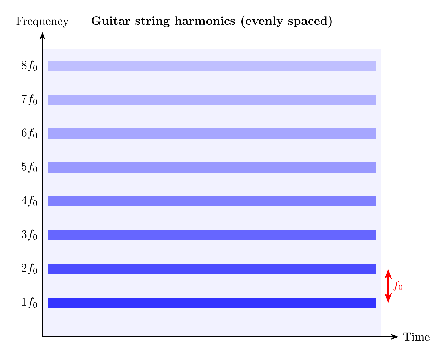
The solution (2.15) shows that the sound of a vibrating string is the sum of multiple (in theory infinite) frequencies. The lowest frequency in the response is called the fundamental frequency. For a stretched string this is \(\frac{\pi c}{\ell}\) rad/s or \(\frac{\pi c}{2\pi\ell}\) Hz. The frequencies above the fundamental frequency are called overtones. Note that the individual frequencies in the response are all integer multiples of the lowest frequency. These overtones are called harmonics.

Harmonics of Piano and Harpsichord
The harmonics of the harpsichord and piano will be compared. The sound in both instruments is produced by vibrations in strings. However, in a harpsichord the string is plucked while in a piano the string is struck. Although the two instruments look superficially quite similar, the sound is quite different. Let’s examine the mathematics of this.
Harpsichord
When one of the keys on the harpsichord’s keyboard is depressed, a mechanism protecting the string pops up, a device plucks the string, and then the mechanism falls back so that the string is only plucked once per keyboard strike. Therefore, the initial position of the string is described by the hat function
\[ f(x) = \begin{cases} \frac{x}{x_0} & 0 \leq x < x_0 \\ \frac{\ell - x}{\ell - x_0} & x_0 \leq x \leq \ell \end{cases} \tag{2.16} \]\(f(x)\), shown in Figure 2.3, while the string has a zero initial velocity. The coefficients of the Fourier sine series of \(f(x)\) were calculated above (see (2.14)) as
\[ A_k = \frac{2}{\ell}\int_0^{\ell} f(x)\sin\left(k\pi\frac{x}{\ell}\right)dx = \frac{2\ell^2}{\pi^2 x_0(\ell - x_0)}\frac{\sin\left(k\pi\frac{x_0}{\ell}\right)}{k^2}. \]Thus, with initial conditions \(u(x,0) = f(x)\) and \(\frac{\partial u}{\partial x}(x,0) = 0\), the deflection of a string (see (2.15)) is
\[ u_p(x,t) = \sum_{k=1}^{\infty} A_k \cos\left(\frac{k\pi ct}{\ell}\right)\sin\left(\frac{k\pi x}{\ell}\right). \tag{2.17} \]Since the coefficients \(A_k\) depend on the point \(x_0\) at which the string is plucked, this implies that the sound of a plucked stringed instrument (guitar, harp, harpsichord, and others) depends heavily on the position at which the string is plucked. This is why some harpsichords employ a mechanism (called a stop) to pluck the strings at different lengths away from the keyboard. This changes the sound of the instrument. Notice in particular that if \(x_0 = \frac{\ell}{2}\),
\[ \begin{aligned} A_{2k} &= \frac{2L^2}{\pi^2 x_0(L - x_0)}\frac{\sin\left(\frac{(2k)\pi x_0}{L}\right)}{(2k)^2} \\ &= \frac{2L^2}{\pi^2 \frac{L}{2}(L - \frac{L}{2})}\frac{\sin\left(\frac{(2k)\pi\frac{L}{2}}{L}\right)}{(2k)^2} \\ &= \frac{2}{\pi^2}\frac{\sin(k\pi)}{k^2} \\ &= 0, \end{aligned} \]since \(\sin(k\pi) = 0\) for \(k \in \mathbb{N}\). Thus, all the even harmonics will be missing.
Piano
In a piano, the taut string lies flat, and a hammer strikes the string when a key is depressed. From this, we gather that the initial position of the string is zero, but when the hammer strikes the string, its initial velocity is non-zero. When the string is struck by the hammer, the graph of its initial velocity takes the shape of the hat function \(f(x)\) shown in Figure 2.3 and defined in (2.16).
Since the initial position is the zero function, \(A_k = 0\) for all \(k\) in the expression for the deflections (2.15). Term-by-term differentiation of (2.15) yields
\[ \frac{\partial u}{\partial t}(x,t) = \sum_{k=1}^{\infty}\frac{\pi k c}{\ell}\left[-A_k\sin\left(\frac{\pi k ct}{\ell}\right) + B_k\cos\left(\frac{\pi k ct}{\ell}\right)\right]\sin\left(\frac{k\pi x}{\ell}\right). \]and since \(A_k = 0\),
\[ \frac{\partial u}{\partial t}(x,0) = f(x) = \sum_{k=1}^{\infty}\frac{\pi k c}{\ell}B_k\sin\left(\frac{k\pi x}{\ell}\right). \tag{2.18} \]Solving for \(B_k\) and using the Fourier series for the hat function calculated in (2.14),
\[ \begin{aligned} B_k &= A_k \frac{\ell}{\pi k c} \\ &= \frac{2\ell^3}{\pi^3 c x_0(\ell - x_0)}\frac{\sin\left(\frac{k\pi x_0}{\ell}\right)}{k^3}. \end{aligned} \]Thus, with initial conditions \(u(x,0) = 0\) and \(\frac{\partial u}{\partial x}(x,0) = f(x)\), the deflection of a string (see (2.15)) is
\[ u(x,t) = \sum_{k=1}^{\infty} B_k \sin\left(\frac{\pi k c}{\ell}t\right)\sin\left(\frac{\pi k}{\ell}x\right). \]Comparison
The Fourier coefficients \(A_k\) of the harpsichord vanish as \(A_k \propto \frac{1}{k^2}\), while the piano’s harmonics vanish as \(B_k \propto \frac{1}{k^3}\). This says that the harpsichord retains more of its higher harmonics than the piano, hence contributing to the vast difference in tone between the two string instruments, simply because of how the strings are sounded (plucked vs struck).
Modes of Vibration
\[ u(x,t) = \sum_{k=1}^{\infty}\left[A_k\cos\left(\frac{\pi k c}{\ell}t\right) + B_k\sin\left(\frac{\pi k c}{\ell}t\right)\right]\sin\left(\frac{\pi k}{\ell}x\right). \]The individual terms \(u_k\) are the modes of vibration of the response. For a vibrating string with fixed ends, each mode of vibration is
\[ u_k(x,t) = (A_k\cos(\omega_k t) + B_k\sin(\omega_k t))\sin\left(\frac{\omega_k}{c}x\right) \]Defining
\[ M_k = \sqrt{A_k^2 + B_k^2}, \quad \sin\phi_k = \frac{A_k}{\sqrt{A_k^2 + B_k^2}}, \quad \cos\phi_k = \frac{B_k}{\sqrt{A_k^2 + B_k^2}}, \]\[ u_k(x,t) = M_k\sin(\omega_k t + \phi_k)\sin\left(\frac{\omega_k}{c}x\right) \]The maximum amplitude of each mode is constant with time. The mode shapes for a vibrating string where deflection \(u = 0\) at each end are
\[ \sin\left(\frac{\omega_k}{c}x\right). \]In a vibrating string, for each mode of vibration beyond the first mode, there are point(s) \(0 < x < \ell\) where the deflection is 0 at all time. Such points are called nodes. The first seven modes are illustrated in Figure 2.8.

Chapter 3: Wind Instruments
The sound in many instruments, such as the clarinet and flute, is made by blowing air into the instrument. Here we consider models where the instrument can be treated as a cylinder much longer than it is wide, so that only one space dimension needs to be considered. This assumption is reasonable for clarinets and flutes.
Consider particles at position \(x\) when undisturbed and denote displacement from the “usual” location \(x\) by \(u(x,t)\). (Think of a slinky.) Denote similarly pressure \(P(x,t)\), density \(\rho(x,t)\). Let \(P_0 = 0\) be the pressure of the undisturbed air and \(\rho_0\) the density. Assume that only motion in the \(x\)-direction is present; then from Newton’s Law on a section \([x, x + \Delta x]\), letting cross-sectional area be \(A\),
\[ \begin{aligned} ma &= F \\ \rho_0 A(x)\Delta x \frac{\partial^2 u}{\partial t^2} &= A(x)P(x,t) - A(x + \Delta x)P(x + \Delta x, t) \end{aligned} \]Assume cross-sectional area \(A\) is constant and divide through by \(A\Delta x\):
\[ \rho_0 \frac{\partial^2 u}{\partial t^2} = -\frac{P(x + \Delta x, t) - P(x,t)}{\Delta x}. \]Taking the limit as \(\Delta x \to 0\) yields
\[ \rho_0 \frac{\partial^2 u}{\partial t^2} = -\frac{\partial P(x,t)}{\partial x}. \tag{3.1} \]An equation in only one variable is needed. Write \(P'(\rho) = \frac{\partial P}{\partial \rho}\). Then the linear approximation to \(P\) as a function of \(\rho\) is, recalling that \(P(\rho_0) = P_0 = 0\),
\[ P(\rho) \approx P'(\rho_0)(\rho - \rho_0). \tag{3.2} \]Also, since \(\rho = \frac{\text{Mass}}{\text{Volume}}\),
\[ \rho(x,t) = \frac{\rho_0 A\Delta x}{A(x + \Delta x + u(x+\Delta x, t) - (x + u(x,t)))} = \frac{\rho_0}{1 + \frac{u(x+\Delta x,t) - u(x,t)}{\Delta x}}. \]Taking the limit as \(\Delta x \to 0\), \(\rho(x,t) = \rho_0(1 + \frac{\partial u}{\partial x})^{-1} \approx \rho_0(1 - \frac{\partial u}{\partial x})\). Substituting into (3.2) yields
\[ P(x,t) \approx -P'(\rho_0)\rho_0 \frac{\partial u}{\partial x}. \tag{3.3} \]Substitute (3.3) into (3.1) to obtain, after dividing by \(\rho_0\) and defining \(c^2 = P'(\rho_0)\),
\[ \frac{\partial^2 u(x,t)}{\partial t^2} = c^2 \frac{\partial^2 u(x,t)}{\partial x^2}. \tag{3.4} \]Same equation as for a stretched string!
The constant \(c\) in equation (3.4) is the speed of sound in the given medium, in this case air. It increases strongly with temperature.
Flute
A flute is essentially a long open tube with constant cross-sectional area, so equation (3.4) applies. Both ends are open, so the pressure \(P(x,t) = P_0 = 0\) at the ends. Using (3.3) this yields the boundary conditions, for a flute of length \(\ell\),
\[ \frac{\partial u}{\partial x}(0,t) = 0, \quad \frac{\partial u}{\partial x}(\ell,t) = 0. \tag{3.5} \]Since (3.4) is the same equation as studied previously for a vibrating string, the same solution procedure can be used. Separation of variables means substituting \(u(x,t) = M(x)N(t)\) into (3.4) and rearranging to obtain
\[ \frac{N''(t)}{c^2 N(t)} = \frac{M''(x)}{M(x)} = -\lambda. \]This yields the differential equation \(M''(x) + \lambda M(x) = 0\), and so with arbitrary constants \(c_1\), \(c_2\),
\[ M(x) = c_1\cos(\sqrt{\lambda}\,x) + c_2\sin(\sqrt{\lambda}\,x). \]But to satisfy the boundary conditions (3.5), \(M'(0) = 0\) and \(M'(\ell) = 0\), so \(c_2 = 0\) and \(\sqrt{\lambda}\,\ell = k\pi\) for \(k = 0, 1, 2, \ldots\) Thus
\[ M(x) = c_1\cos\left(\frac{k\pi}{\ell}x\right). \]Defining \(\omega_k = \frac{k\pi c}{\ell}\), the time equation \(N''(t) + \omega_k^2 N(t) = 0\) has general solution \(N(t) = A_k\cos(\omega_k t) + B_k\sin(\omega_k t)\). The full solution is
\[ u(x,t) = \sum_{k=1}^{\infty}(A_k\cos(\omega_k t) + B_k\sin(\omega_k t))\cos\left(\frac{\omega_k}{c}x\right), \quad \omega_k = \frac{k\pi c}{\ell} \]where \(A_k\), \(B_k\) are chosen so initial conditions are satisfied. The fundamental frequency is the lowest frequency present:
\[ \frac{\pi c}{\ell} \text{ rad/s}, \quad \frac{c}{2\ell} \text{ Hz}. \]The parameter \(c\) depends on temperature, weakly on humidity. For dry air, \(c = 342\) m/s (20°C), \(c = 345\) m/s (25°C). Using \(c = 344\) m/s,
| Instrument | Length (m) | Theo. pitch (Hz) | Actual pitch (Hz) |
|---|---|---|---|
| flute | 0.66 | 260 | 262 |
| short tube | 0.3 | 573 | 524 |
| long tube | 0.63 | 273 | 262 |
Length clearly corresponds to pitch. The errors, which are more significant for shorter tubes, are due primarily to end effects: the pressure is not zero exactly at the ends, but drops to zero at a small distance from the end.
Different notes can be produced by opening and covering various holes, thus changing the effective length of the instrument. This is the case for many woodwind instruments, such as oboe, clarinet, saxophone, and flute. On the flute and many other instruments, different notes are also produced, without changing the fingering, by exciting various overtones or resonant frequencies of the instrument.
The analysis predicts that the frequencies \(\omega_k = \frac{k\pi c}{\ell}\) are present. Writing the fundamental at \(\omega_1\), the overtones are integer multiples of the fundamental:
\[ \omega_2 = 2\omega_1, \quad \omega_3 = 3\omega_1, \ldots \]Overtones that occur as integer multiples of the fundamental are also called harmonics.

Clarinet
A clarinet has a reed made of thin cane at the mouthpiece. The player blows into the mouthpiece, causing the reed to vibrate. As the reed bends under the pressure of the airstream, it behaves as a spring, repeatedly closing and opening the mouthpiece. This back-and-forth motion produces vibrations in the air column at the mouthpiece. As with the flute, this initial motion then causes the air column trapped in the clarinet body to vibrate at its natural frequency. The reed is forced by the air column and vibrates at the same frequency.
The wave equation also applies to sound waves in a clarinet. Key facts:
- About the same length as a flute
- Also a cross-section that is approximately constant
- End (\(x = \ell\) is open
Sound is produced by vibration of the reed against the mouthpiece and pressure at \(x = 0\) is not zero. The small opening and the fluctuations where the reed closes the opening mean that an appropriate set of boundary conditions is
\[ u(0,t) = 0, \quad \frac{\partial u}{\partial x}(\ell, t) = 0. \tag{3.6} \]Separation of variables again is used to solve the wave equation, but now the spatial function \(M\) must satisfy \(M''(x) + \lambda M(x) = 0\) with \(M(0) = 0\), \(M'(\ell) = 0\). Solving yields
\[ M(x) = c_2\sin(\sqrt{\lambda_k}\,x) \]where \(\sqrt{\lambda_k} = (k - \frac{1}{2})\frac{\pi}{\ell} = \frac{(2k-1)\pi}{2\ell}\), \(k = 1, 2, \ldots\) so that \(M'(\ell) = 0\).
Defining \(\omega_k = \sqrt{\lambda_k}\,c = \frac{(2k-1)\pi c}{2\ell}\), the solution is
\[ u(x,t) = \sum_{k=1}^{\infty}(A_k\cos(\omega_k t) + B_k\sin(\omega_k t))\sin\left(\frac{\omega_k}{c}x\right) \]The predicted fundamental frequency is
\[ \omega_1 = \sqrt{\lambda_1}\,c = \frac{\pi c}{2\ell} = \frac{c}{4\ell} \text{ Hz} \]| Instrument | Length (m) | Theo. pitch (Hz) | Actual pitch (Hz) |
|---|---|---|---|
| clarinet | 0.6 | 143 | 147 (D3) |
| flute | 0.66 | 260 | 262 (C4) |
| closed short red tube | 0.3 | 286 | 262 (C4) |
| open short red tube | 0.3 | 573 | 524 (C5) |
| open long red tube | 0.63 | 273 | 262 (C4) |
Two key observations:
- The fundamental of the tube with one end closed is half that of the open tube, as predicted by theory.
- The clarinet is about the same length as a flute but the fundamental frequency is nearly half that of a flute.
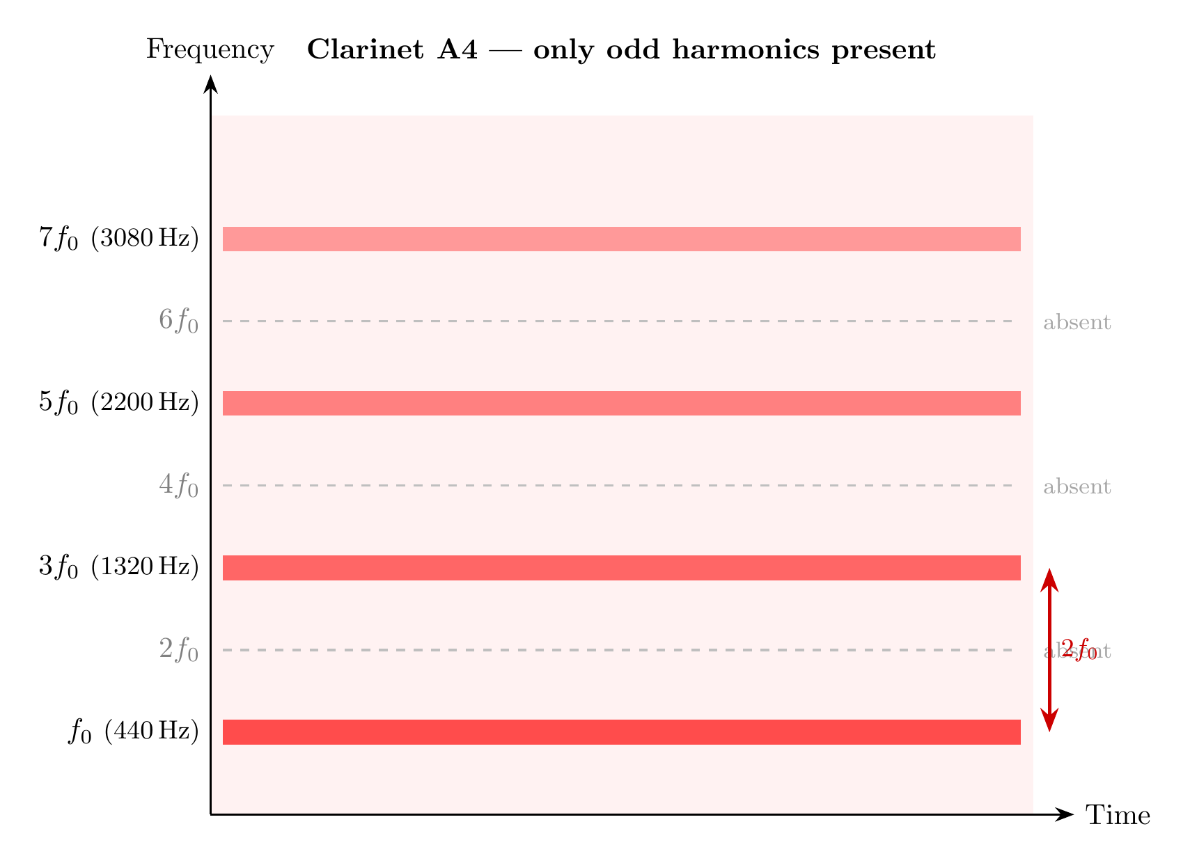
The analysis predicts that the frequencies \(\omega_k = \frac{(2k-1)c}{4\ell}\) are present. Writing the fundamental at \(\omega_1 = \frac{c}{4\ell}\):
\[ \omega_2 = 3\omega_1, \quad \omega_3 = 5\omega_1, \ldots \]Although these overtones are harmonics, only the odd harmonics are present. This is reflected in the spectrogram of a clarinet.

Vocabulary
Fundamental (frequency) — lowest frequency of a note/sound. Generally the perceived pitch.
Overtones — frequencies above the fundamental frequency. The first component above the fundamental is the first overtone.
Harmonics — overtones that are at integer multiples of the fundamental.
Partials — the \(m\)th partial is the \(m\)th frequency component present. The fundamental frequency is the first partial.
Pitch — perceived frequency of a sound; generally the fundamental frequency (20Hz–20,000Hz is the range audible to humans).
Timbre — determined strongly by frequencies present in a sound; in particular overtones and their relative strength. Transients also affect timbre.
Amplitude — magnitude of vibration; corresponds to loudness.
Duration — length of time a note sounds.
As an example of using these terms, consider a clarinet:
- Fundamental frequency \(\frac{c}{4\ell}\); also the first harmonic
- Second harmonic \(\frac{2c}{4\ell}\) is not present
- \(\frac{3c}{4\ell}\) is the third harmonic or first overtone
More Complex Models
The simplest model for oboes, saxophones, and brass instruments is a tube of varying cross-section. The wave equation becomes
\[ \frac{\partial^2 u(x,t)}{\partial t^2} = \frac{c^2}{A(x)}\frac{\partial}{\partial x}\left(A(x)\frac{\partial u(x,t)}{\partial x}\right). \]For some profiles \(A(x)\) this equation can be solved theoretically using separation of variables, but the calculations are more complicated. The precise profile \(A(x)\) affects the fundamental frequency and the overtones. For example, soprano saxophone and clarinet are about the same length, and look similar, but soprano saxophone has a conical profile. The fundamental of a clarinet is almost an octave lower, and the timbre is quite different.
For many instruments, a two- or three-dimensional model needs to be considered because the sound waves travel in more than one direction. Nonlinearities are also often important. For some instruments, such as oboes, other effects such as the vibrations of the reed are important and accurate mathematical models are difficult. Complex models are needed to model the acoustic response of vocal folds and the associated throat area.
Chapter 4: Drums
A drum is a membrane stretched over a frame and fixed at the frame. Only a model for a simple drum — that is, a single membrane with no enclosure — will be developed. A bodhrán is an example of this type of drum. Assuming gravity is negligible compared to the tension, Newton’s Law applied to a small region gives
\[ \rho\Delta x\Delta y\frac{\partial^2 u}{\partial t^2} = \text{Force of Tension} \]where \(\rho\) is mass per unit area (kg/m²). The governing equation for a vibrating string was derived assuming constant density, a perfectly flexible string, no resistance, friction or other dissipative forces, and small deflections so nonlinearities are neglected.
Applying these same assumptions to a stretched membrane, and using the same technique as for a string (but with vector calculus), leads to the 2D wave equation. Defining \(c^2 = \frac{T}{\rho}\) where \(T\) is tension (force per unit length, N/m):
\[ \frac{\partial^2 u}{\partial t^2} = c^2\left(\frac{\partial^2 u(x,t)}{\partial x^2} + \frac{\partial^2 u(x,t)}{\partial y^2}\right), \quad (x,y) \in \Omega \]with boundary condition \(u(x,y,t) = 0\) for \((x,y) \in \partial\Omega\).
Typically \(\Omega\) is a disk of radius \(a\). Since \(\Omega\) is a disc, polar coordinates are natural. Using \(x = r\cos\theta\), \(y = r\sin\theta\), the wave equation in polar coordinates is
\[ \frac{\partial^2 u}{\partial t^2} = c^2\left(\frac{1}{r}\frac{\partial}{\partial r}\left(r\frac{\partial u}{\partial r}\right) + \frac{1}{r^2}\frac{\partial^2 u}{\partial\theta^2}\right) \]Since the membrane is fixed around the edges and is a continuous material, the boundary conditions are
\[ u(r, 0, t) = u(r, 2\pi, t) = 0, \quad u(a, \theta, t) = 0, \quad u(0, \theta, t) < \infty \]Separation of Variables in Polar Coordinates
Since there are 3 variables, try \(u(r, \theta, t) = R(r)\Theta(\theta)T(t)\). Substituting into the wave equation and rearranging yields
\[ \frac{T''}{c^2 T} = \left[\frac{1}{rR}(rR')' + \frac{1}{r^2}\frac{\Theta''}{\Theta}\right] = -\lambda^2 \tag{4.1} \]since \(t\), \(r\), \(\theta\) are independent. This gives \(T'' + c^2\lambda^2 T = 0\), the same oscillator equation obtained previously, so
\[ T(t) = A_n\cos(c\lambda t) + B_n\sin(c\lambda t). \]Rearranging (4.1),
\[ \frac{r}{R}(rR')' + \lambda^2 r^2 = -\frac{\Theta''}{\Theta}. \]Since the left side depends only on \(r\) and the right side only on \(\theta\), each must equal a constant \(\mu^2\). Thus:
\[ \Theta'' + \mu^2\Theta = 0 \]\[ (rR')' + \lambda^2 rR - \frac{\mu^2}{r}R = 0 \]The equation for \(\Theta\) is the oscillator equation. For periodicity with period \(2\pi\), we need \(\mu = n\), \(n = 0, 1, 2, \ldots\)
Bessel Functions
The equation for \(R\) is a new differential equation. Any solution has the form, for constants \(D_n\), \(E_n\),
\[ R(r) = D_n J_n(\lambda r) + E_n Y_n(\lambda r) \]where \(J_n\), \(Y_n\) are \(n\)th-order Bessel functions of the first and second kind respectively. Since the Bessel functions of the second kind \(Y_n\) are unbounded at \(r = 0\), \(E_n = 0\) for all \(n\) and
\[ R(r) = D_n J_n(\lambda r). \]The boundary conditions also imply \(R(a) = 0 = J_n(\lambda a)\).
For each \(n\), \(J_n\) has an infinite number of zeros. This yields the values of \(\lambda_{n,m}\), \(m = 1, 2, \ldots\) The zeros of the Bessel functions \(J_n\) have some important properties:
- Each \(J_n\) has an infinite number of zeros, approaching infinity.
- Except for \(r = 0\), \(J_n\) and \(J_m\), \(n \neq m\), have no zeros in common.
- The zeros are not evenly spaced.

Solution for the Drum
Assuming zero initial velocity, the deflections \(u\) of a stretched round membrane are
\[ u(r,\theta,t) = \sum_{m=1}^{\infty}\sum_{n=0}^{\infty}(A_{nm}\cos(n\theta) + B_{nm}\sin(n\theta))J_n(\lambda_{n,m}r)\cos(c\lambda_{n,m}t) \]where \(\lambda_{n,m}\) are such that \(J_n(\lambda_{n,m}a) = 0\).
The natural frequencies of vibration are \(c\lambda_{n,m}\) where \(\lambda_{n,m}\) are zeros of \(J_n\). Because the zeros of \(J_n\) are not evenly spaced, a round drum has overtones, but they are not harmonics. This is why drums do not produce a clear sense of pitch in the same way that stringed or wind instruments do.
The mode shape — the spatial part of the response for the mode \((n, m)\) — is of the form
\[ \cos(n\theta)J_n(\lambda_{n,m}r). \]Some mode shapes depend only on \(\theta\), some only on \(r\), most on both. Except for the first mode, each mode has nodal lines or curves where the deflection is always zero. These nodal lines are called Chladni patterns.
Chapter 5: Idiophones
In these instruments, the sound is produced by striking a bar. This sets up transverse vibrations in the bar, which are different from the longitudinal vibrations that occur in a tube or string.
The force is due to a moment on each element of the bar. Under certain assumptions (no twisting, linearity, constant physical parameters), the governing differential equation is
\[ \rho\frac{\partial^2 u}{\partial t^2}(x,t) + EI\frac{\partial^4 u}{\partial x^4}(x,t) = 0, \quad 0 < x < \ell \tag{5.1} \]where \(E\), \(I\), \(\rho\) are physical parameters. Since they are constant, define \(c^2 = \frac{EI}{\rho}\) (m⁴/s²) which yields
\[ \frac{\partial^2 u}{\partial t^2}(x,t) + c^2\frac{\partial^4 u}{\partial x^4}(x,t) = 0. \tag{5.2} \]Equation (5.1) or (5.2) is known as the Euler–Bernoulli beam equation, or often just the beam equation. Various boundary conditions are possible, depending on how the bars are fastened.
Separation of Variables
Assuming a solution of the form \(u(x,t) = M(x)T(t)\), substituting into the beam equation and rearranging yields
\[ \frac{T''}{T} = -c^2\frac{M^{IV}}{M} \]where \(M^{IV}\) indicates the 4th derivative. The equation for \(T\) is the familiar harmonic equation \(T'' + \omega^2 T = 0\) with solution
\[ T(t) = A\cos\omega t + B\sin\omega t. \]The spatial function \(M(x)\) must satisfy the fourth-order ordinary differential equation
\[ M^{IV} = \frac{\omega^2}{c^2}M. \]Since this is 4th order, the general solution involves 4 functions. Defining \(\kappa = \left(\frac{\omega^2}{c^2}\right)^{1/4} = \left(\frac{\omega}{c}\right)^{1/2}\), it is straightforward to verify that for arbitrary constants \(A\), \(B\), \(C\), \(D\),
\[ M(x) = A\sin\kappa x + B\cos\kappa x + C\sinh\kappa x + D\cosh\kappa x \]solves the differential equation.
Clamped–Free Boundary Conditions
Suppose one end is clamped and the other free. This situation occurs in mbira and some other instruments. Mathematically, this means
\[ u(0,t) = 0, \quad \frac{\partial u}{\partial x}(0,t) = 0, \quad \frac{\partial^2 u}{\partial x^2}(\ell,t) = 0, \quad \frac{\partial^3 u}{\partial x^3}(\ell,t) = 0 \tag{5.3} \]From the boundary conditions at \(x = 0\), \(B + D = 0\) and \(A + C = 0\), so
\[ M(x) = A(\sin\kappa x - \sinh\kappa x) + B(\cos\kappa x - \cosh\kappa x). \]Using the other 2 boundary conditions leads to the linear system
\[ \begin{bmatrix} (-\sin\kappa\ell - \sinh\kappa\ell) & (-\cos\kappa\ell - \cosh\kappa\ell) \\ (-\cos\kappa\ell - \cosh\kappa\ell) & (\sin\kappa\ell - \sinh\kappa\ell) \end{bmatrix}\begin{bmatrix} A \\ B \end{bmatrix} = \begin{bmatrix} 0 \\ 0 \end{bmatrix} \tag{5.4} \]This has non-trivial solutions only if the determinant is zero:
\[ 1 + \cos\kappa\ell\cosh\kappa\ell = 0. \tag{5.5} \]Natural Frequencies
The natural frequencies predicted by this model are \(\omega_j = \kappa_j^2 c\) where \(\kappa_j\) solves (5.5). Now,
\[ 1 + \cos z\cosh z = 1 + \frac{1}{2}\cos z(e^z + e^{-z}) \]and so for large \(z\), \(1 + \cos z\cosh z \approx \frac{1}{2}(\cos z)e^z\). Thus, the zeros of \(1 + \cos z\cosh z\) approach those of \(\cos z\) and so
\[ \kappa_j \approx \frac{(2j-1)\pi}{2}. \]| Natural frequencies | Harmonic approximation |
|---|---|
| 3.52 | 2.47 |
| 22.0 | 22.0 |
| 61.7 | 61.7 |
| 121 | 121 |
Even the first overtone is very close to this harmonic approximation. This is typical of idiophones.
This model neglects a number of factors affecting the sound of idiophones. The pitch and timbre of bars in idiophones are often tuned by shaping the bar; cutting out a notch is common. This can only be modelled by including factors such as torsion (twisting) and thickness. As for drums, some idiophones — for instance the marimba — have a resonator that serves to accentuate certain overtones and reduce others. Also, actual instruments have dissipation and different modes decay at different rates. This transient effect contributes to the timbre of an instrument. Transients are present in all instruments, but their effect on the timbre of idiophones is particularly significant.
Chapter 6: Frequency Response and Sampling
The first five chapters of this course developed mathematical models for families of musical instruments: strings, wind instruments, drums, and idiophones. These models predict the pitch and overtone structure of each instrument. We now turn to a different but equally important topic: the mathematical framework for analyzing how systems respond to periodic signals, and how continuous sounds can be faithfully captured and reconstructed from discrete samples. These ideas underpin digital audio recording and reproduction.
Frequency Response
Consider the first-order differential equation with a forcing function \(u\):
\[ \dot{z}(t) = -az(t) + bu(t), \quad a > 0, \quad z(0) = z_o. \tag{6.1} \]This describes a number of physical situations. For instance, \(z\) can be the temperature of a well-mixed tank and \(u\) is the heat added or removed. The solution to this differential equation is
\[ z(t) = e^{-at}z_o + \int_0^t e^{-a(t-\tau)}bu(\tau)\,d\tau. \]For large time, the initial condition decays and
\[ \lim_{t\to\infty} z(t) = \int_0^t e^{-a(t-\tau)}bu(\tau)\,d\tau. \]The response for large time is entirely due to the forcing function. This is called the steady-state response.
Consider a periodic forcing term \(u\). It is easier to integrate an exponential than a sine or cosine. Using the notation \(i = \sqrt{-1}\), Euler’s formula states that for real \(\omega\),
\[ e^{i\omega} = \cos\omega + i\sin(\omega). \]It follows that
\[ \cos(\omega) = \frac{1}{2}(e^{i\omega} + e^{-i\omega}), \quad \sin(\omega) = \frac{1}{2i}(e^{i\omega} - e^{-i\omega}). \]With the complex exponential input \(u(t) = e^{i\omega t}\), the solution becomes
\[ z(t) = e^{-at}z_o + \frac{-be^{-at}}{a + i\omega} + \frac{be^{i\omega t}}{a + i\omega}. \]As \(t \to \infty\), the first two terms become insignificant. The steady-state response is
\[ z_{ss}(t) = \frac{be^{i\omega t}}{a + i\omega}. \tag{6.2} \]Note that the magnitude of this response is
\[ |z_{ss}(t)| = \frac{b}{\sqrt{a^2 + \omega^2}}. \]Since \(\cos(\omega t) = \text{Re}\,e^{i\omega t}\), the steady-state response to a cosine forcing is the real part of (6.2). This works out to
\[ \frac{b(a\cos(\omega t) + \omega\sin(\omega t))}{a^2 + \omega^2}, \]or, defining \(\phi = -\arctan(\frac{\omega}{a})\),
\[ \frac{b}{\sqrt{a^2 + \omega^2}}\cos(\omega t + \phi). \]For small forcing frequencies, the phase shift \(\phi \approx 0\) and the response is about \(\frac{b}{a}\). As \(\omega\) increases, the phase shift \(\phi\) decreases to \(-90\) degrees and the magnitude decreases to 0. A plot of the response of a system to a periodic forcing function as the frequency of the forcing function changes is called the frequency response.
More generally, defining \(f(t) = e^{-at}b\), the steady-state response to a forcing function \(u\) is described by the convolution
\[ \int_0^t f(t - \tau)u(\tau)\,d\tau. \]This generalizes to systems of ordinary differential equations and also systems modelled by partial differential equations, such as a vibrating string or pressure waves.
The Fourier Transform
Let \(f\) now be the impulse response of some system so that the effect of an input \(u\) on some quantity \(y\) is described by, for large \(t\) or with zero initial condition,
\[ y(t) = \int_0^t f(t-\tau)u(\tau)\,d\tau. \]If \(u(t) = e^{i\omega t}\), then
\[ y(t) = \int_0^t f(\tau)e^{i\omega(t-\tau)}\,d\tau = e^{i\omega t}\int_0^t f(\tau)e^{-i\omega\tau}\,d\tau \approx e^{i\omega t}\int_{-\infty}^{\infty} f(\tau)e^{-i\omega\tau}\,d\tau. \]With frequency \(\omega = 2\pi\nu\) where \(\nu\) is the frequency in Hertz, defining
\[ \hat{f}(\nu) = \int_{-\infty}^{\infty} f(\tau)e^{-i2\pi\nu\tau}\,d\tau, \]the steady-state response can be rewritten as \(y(t) = \hat{f}(\nu)e^{i2\pi\nu t}\). The function \(\hat{f}(\nu)\) is the frequency response, or equivalently, the Fourier transform.
The Fourier transform of a real (or complex)-valued function \(f\) of a real variable \(t\) is defined as
\[ \hat{f}(\nu) = \int_{-\infty}^{\infty} f(t)e^{-2\pi i\nu t}\,dt \tag{6.3} \]for any function for which the integral is well-defined. There are many slightly different definitions of the Fourier transform; they vary in their handling of constants but are fundamentally all equivalent.
Clearly the Fourier transform of any function that is only non-zero on a bounded interval and integrable on that interval is well-defined. In fact, if \(\int_{-\infty}^{\infty}|f(t)|\,dt < \infty\), the Fourier transform is defined.
Conversely, a function of \(t\) can be uniquely constructed from the Fourier transform, or frequency response.
Theorem (Inverse Fourier Transform). Let \(f\) be a piecewise smooth function that is also integrable on \((-\infty, \infty)\). At points where \(f\) is continuous,
\[ f(t) = \int_{-\infty}^{\infty}\hat{f}(\nu)e^{2\pi i\nu t}\,d\nu. \tag{6.4} \]At discontinuities, the value of the above integral is the average of the right and left limits of \(f\).
There is thus a one-to-one correspondence between a function \(f(t)\) and its Fourier transform \(\hat{f}(\nu)\). Since the transform is defined via an integral, it is linear: if \(a\) is a scalar and \(f\), \(g\) have Fourier transforms, then \(\widehat{(af + g)}(\nu) = a\hat{f}(\nu) + \hat{g}(\nu)\). Similarly, the inverse Fourier transform is also linear.
The Nyquist Sampling Theorem
In practice, the frequency response of a signal or sound \(f(t)\) is calculated by recording it at a finite number of time instants \(\{f(nT)\}\) where \(T\) is the time between samples. This set of samples is used to obtain the frequency response. It is also used in digital sound reproduction: the samples are stored in memory and reconstructed. Clearly it is possible to recover a sound that sounds to our ears like the original, but how often must the sound be sampled?
Theorem (Nyquist Sampling Theorem). Suppose a Fourier-transformable function \(f\) has the property that its Fourier transform is band-limited; that is,
\[ \hat{f}(\nu) = 0, \quad |\nu| > \sigma. \]Then \(f\) can be recovered exactly from its samples, provided that the sampling rate \(N > 2\sigma\). In this case, defining \(T = \frac{1}{N}\),
\[ f(t) = \sum_{n=-\infty}^{\infty} Tf(nT)\frac{\sin(2\pi\sigma(t - nT))}{\pi(t - nT)}. \tag{6.5} \]If sound is sampled at a rate less than the Nyquist rate, a phenomenon called aliasing occurs where frequencies beyond half the sampling rate get distorted into the lower band and the sound is not correctly reconstructed.
Connection between Fourier Series and Fourier Transform
There is a close connection between Fourier series and Fourier transforms. Consider a real-valued function \(f(t)\) with, for some fundamental frequency \(\omega_0\) (rad/s), the Fourier series
\[ \tilde{f}(t) = a_0 + \sum_{n=1}^{\infty}(a_n\cos(n\omega_0 t) + b_n\sin(n\omega_0 t)). \tag{6.6} \]The individual terms are called harmonics. The period of \(\tilde{f}\) is \(T = \frac{2\pi}{\omega_0}\). The fundamental frequency in Hz is \(\frac{\omega_0}{2\pi}\) or \(\frac{1}{T}\). Series of this form occurred when solving the wave equation for the response of vibrating strings and wind instruments.
It is convenient to use the exponential form of the Fourier series. Defining \(c_n = \frac{a_n - ib_n}{2}\) and \(c_{-n} = \frac{a_n + ib_n}{2}\),
\[ \tilde{f}(t) = \sum_{n=-\infty}^{\infty} c_n e^{in\omega_0 t}. \tag{6.7} \]Multiplying both sides by \(e^{-im\omega_0 t}\) and integrating over one period yields
\[ c_m = \frac{1}{T}\int_{-T/2}^{T/2}\tilde{f}(t)e^{-im\omega_0 t}\,dt. \tag{6.8} \]Consider now a function \(f(t)\) defined on the whole real line. If \(f\) is periodic with period \(T\), then a Fourier series can be defined that equals \(f\). However, many functions are not periodic. Consider the function on some interval \([-\frac{T}{2}, \frac{T}{2}]\) and use this to define the Fourier series. The corresponding Fourier series \(\tilde{f}_T\) will have period \(T\). It will equal \(f\) on that interval, but not generally outside it. Defining the integral
\[ \hat{f}(\omega) = \int_{-T/2}^{T/2} f(t)e^{-i2\pi\omega t}\,dt, \]the Fourier coefficients can be written \(c_n = \frac{1}{T}\hat{f}(\frac{n}{T})\). Substituting into (6.7),
\[ \tilde{f}_T(t) = \frac{1}{T}\sum_{n=-\infty}^{\infty}\hat{f}\left(\frac{n}{T}\right)e^{-i2\pi\frac{n}{T}t}. \]Defining \(\Delta = \frac{2\pi}{T}\), this can be rewritten as
\[ \tilde{f}_T(t) = \frac{1}{2\pi}\sum_{n=-\infty}^{\infty}\hat{f}\left(\frac{1}{2\pi}n\Delta\right)e^{-in\Delta t}\Delta. \]This is a Riemann sum. Taking \(\Delta \to 0\) (or equivalently, \(T \to \infty\) yields
\[ \frac{1}{2\pi}\int_{-\infty}^{\infty}\hat{f}\left(\frac{1}{2\pi}\omega\right)e^{i\omega t}\,d\omega. \]Defining \(\nu = \frac{1}{2\pi}\omega\), a change of variables leads to
\[ f(t) = \int_{-\infty}^{\infty}\hat{f}(\nu)e^{2\pi i\nu t}\,d\nu, \]where \(\hat{f}\) is calculated as the integral in (6.3) as \(T \to \infty\). This is exactly the Fourier transform (or frequency response), and the above equation is the inverse relationship. In other words, the Fourier transform arises naturally as the limiting case of the Fourier series when the period is taken to infinity.
Chapter 7: Pythagorean and Just Scales
The Harmonic Series and Scale Construction
Recall that the fundamental frequency of a sound made by an instrument is the pitch. For convenience in reproducing music from one place to another, a pitch is given a name. Note names and the pitch associated with them vary between cultures and also in time. For example, consider the note A in the treble clef (A4): A4 is now standard at 440 Hz in North America, often slightly higher in continental Europe, and in the Baroque era was significantly lower and varied considerably. The crucial point is that all musicians in the room have the same sound corresponding to a given note name. Furthermore, how notes relate to other notes is critical.
Most music has a “home” note, called the tonic or sometimes do, about which the piece revolves. Most musical pieces are composed with a specified set of notes built on the tonic. This choice of notes is called a scale. An octave is the frequency double the tonic, and most scales are octave-based. For string and wind instruments, overtones occur in integer multiples of the fundamental frequency. Both amplitude and frequency are perceived on a logarithmic scale.
Although the models developed in the first part of the course neglect many aspects of instruments’ behaviour, they do correctly predict the pitch (fundamental frequency) and that the overtones are harmonic, that is, they are integer multiples of the fundamental frequency.
Consider a string with fundamental frequency \(f\); call this the tonic or do. Another string with half the length has frequency \(2f\) (the first overtone). All the harmonics of \(2f\) are contained in the harmonics of \(f\), so the sound from two such strings sounds harmonious. The ancient Greeks noticed that strings in the ratio of \(\frac{3}{2}\) also sounded good together: \(\frac{3}{2}f\). Half of the harmonics of \(\frac{3}{2}f\) are contained in those of \(f\). This interval is called a fifth, also known as so.
The Pythagorean Scale
The Pythagorean scale is constructed by filling in notes through iteration on \(\frac{3}{2}f\), dropping by an octave whenever the note exceeds \(2f\). Letting \(f = 1\), the successive applications of the \(\frac{3}{2}\) ratio yield
\[ \frac{3}{2}, \quad \frac{3^2}{2^2}\cdot\frac{1}{2}, \quad \frac{3^3}{2^4}, \quad \frac{3^4}{2^5}\cdot\frac{1}{2}, \quad \frac{3^5}{2^7}. \]Sorting these between 1 and 2 gives the Pythagorean scale:
| do | re | mi | fa | so | la | ti | do |
|---|---|---|---|---|---|---|---|
| \(1\) | \(\frac{9}{8}\) | \(\frac{81}{64}\) | \(\frac{4}{3}\) | \(\frac{3}{2}\) | \(\frac{27}{16}\) | \(\frac{243}{128}\) | \(2\) |
The intervals between successive notes are:
\[ \frac{9}{8} \quad \frac{9}{8} \quad \frac{256}{243} \quad \frac{9}{8} \quad \frac{9}{8} \quad \frac{9}{8} \quad \frac{256}{243} \]giving the pattern big – big – small – (big) – big – big – small. Note that \(\frac{9}{8} = 1.125\) and \(\left(\frac{256}{243}\right)^2 = 1.1098 \approx \frac{9}{8}\).

All the harmonics of \(2f\) are in common with those of \(f\). Half of the harmonics of \(\frac{3}{2}f\) are in common with those of \(f\), and one-third of the harmonics of \(\frac{4}{3}f\) are in common with those of \(f\). However, most of the notes in the Pythagorean scale are in ratios of large numbers of the root note. One-quarter of the harmonics of \(\frac{5}{4}\) are in common with those of \(f\); this ratio is close to \(\frac{81}{64}\) but not equal. As a result, intervals other than the octave, fourth, and fifth can sound discordant, and sounds from the same scale often do not sound harmonious together. This limits polyphony – the practice of playing multiple notes simultaneously.
Just Intonation
Just intonation addresses the problem of discordant intervals by creating a scale using low ratios:
| do | re | mi | fa | so | la | ti | do |
|---|---|---|---|---|---|---|---|
| \(1\) | \(\frac{9}{8}\) | \(\frac{5}{4}\) | \(\frac{4}{3}\) | \(\frac{3}{2}\) | \(\frac{5}{3}\) | \(\frac{15}{8}\) | \(2\) |
The interval between the third note and the root (do–mi) is called a third; the fourth, fifth, and sixth are defined similarly. The ratios for a third, fourth, fifth, and sixth are all low, and notes sound harmonious together.
Starting on the tonic (do), the ratio of do–mi–so is \(1 : \frac{5}{4} : \frac{3}{2}\), or equivalently \(4:5:6\). Starting on the fourth (fa), we have \(\frac{4}{3} : \frac{5}{3} : 2\), also \(4:5:6\). Setting the remaining intervals so that starting on so (the fifth), \(\frac{3}{2} : x : y\) is also in the ratio \(4:5:6\) leads to \(x = \frac{15}{8}\) and \(y = \frac{9}{4}\) (or \(\frac{9}{8}\) in the next octave down).
The intervals in the just scale are:
\[ \frac{9}{8} \quad \frac{10}{9} \quad \frac{16}{15} \quad \frac{9}{8} \quad \frac{10}{9} \quad \frac{9}{8} \quad \frac{16}{15} \]The scale does not have the same tone–tone–semitone pattern as the Pythagorean scale. A chord is several notes played at the same time to produce an effect, and a triad is a chord with three different notes. Movement through chords is an important part of Western music.
Just intonation has more chords with low ratios than the Pythagorean scale. The triads on do, fa, and so (I, IV, V) are in ratios of \(4:5:6\) – they are “justly” tuned. However, not all chords work: the note re (II) has a fifth of \(\frac{5/3}{9/8} = \frac{40}{27} \neq \frac{3}{2}\), meaning the triad built on re is not a pure fifth. This fundamental limitation motivates the search for other tuning systems.


Chapter 8: Transposition
The problem of transposition – changing the home note of a scale while preserving the relationships between notes – reveals deep mathematical constraints on any tuning system. In this chapter, we examine why no fixed-pitch tuning system can simultaneously achieve perfect harmony and unlimited transposability, and how different compromises have been reached throughout history.
The Pythagorean Comma
The Pythagorean scale can be created either by using the recursion formula (\(\frac{3}{2}\), modulo 2) or by intervals. If we create a new scale by transposing up a fifth – that is, taking the tonic to have frequency \(\frac{3}{2}\) and building the same interval pattern on it – we obtain the notes of the original scale except for one new note. Each transposition introduces a new note that was not present before.
Going up 12 fifths is close to 7 octaves. The difference is
\[ \frac{(\frac{3}{2})^{12}}{2^7} = \frac{3^{12}}{2^{19}} \approx 1.014. \]This small discrepancy is called the Pythagorean comma. Each time a scale is created by transposition – starting a new note, either a fifth up or a fifth down from the previous scale – a new note is introduced. This creates what is known as the spiral of fifths: transposition into a scale with a different tonic creates new notes in a never-ending spiral.

The fundamental impossibility can be stated precisely: we need integers \(n, m\) such that
\[ \left(\frac{3}{2}\right)^m = 2^n, \quad \text{i.e.,} \quad 3^m = 2^{n+m}. \]But this requires a power of 3 to equal a power of 2, which is not possible since 3 and 2 are distinct primes. It is therefore impossible to go up a number of perfect fifths and eventually return to the original note, modulo an octave. All temperaments will be a compromise.


Transposition is even worse in just intonation. Starting on the fifth note “G” (frequency \(\frac{3}{2}\) and building a just scale with the same ratios yields two new notes for each transposition, and the spiral of fifths expands even more rapidly.
Meantone Scales
Meantone scales were common in the Renaissance as a compromise that preserves consonances of the octave, fifth, third, and sixth while allowing transposition into different keys and chord progressions. The fundamental idea is to improve thirds over the Pythagorean scale while sacrificing fifths slightly.
One meantone scale is constructed as follows. Ensure that thirds on C, F, and G (I, IV, V) are “just”: \(\frac{5}{4}\). Take the interval within these thirds to be the geometric mean: \(\frac{\sqrt{5}}{2}\). This yields C–D–E as \(1 : \frac{\sqrt{5}}{2} : \frac{5}{4}\), with the same ratios for F–G–A and G–A–B. To keep a Pythagorean scale pattern, two semitones are left, determined by
\[ \left(\frac{\sqrt{5}}{2}\right)^5 s^2 = 2, \]so the semitone is \(s = \frac{8}{5^{5/4}}\).
The fifth in this system is \(r = 5^{1/4} = 1.49535 \approx \frac{3}{2}\). Transposing four fifths is a third (modulo octaves), and 12 fifths is 3 thirds. Since \(\left(\frac{5}{4}\right)^3 = \frac{125}{64} < 2\), we do not get a cycle of fifths. One fifth is usually made large in a seldom-used key, yielding a very discordant wolf fifth. It was possible that a keyboard was tuned differently for different pieces.
Various modifications of meantone make it easier to play in different keys, with intervals slightly different in different keys so the spiral of fifths becomes a circle, but far-away keys have discordant intervals. Because the intervals are different, different keys have noticeably different character. Such tunings are sometimes called well-tempered. Many different schemes existed, with Werckmeister’s being particularly popular. Well-tempered tuning was commonly used until roughly 1850–1900.


Equal Temperament
In the Pythagorean scale, going up 12 fifths and then down 7 octaves goes back to almost where you started: \((\frac{3}{2})^{12} \approx 2^7\). The major scale has 5 tones and 2 semitones, yielding 12 semitones total. However, a Pythagorean tone is not exactly 2 semitones:
\[ \frac{(\frac{256}{243})^2}{\frac{9}{8}} = \frac{2^{16}}{3^{10}} \cdot \frac{3^2}{2^3} = \frac{2^{19}}{3^{12}}. \]Equal temperament resolves all transposition problems by setting each semitone to \(s = 2^{1/12}\), so a tone is \(s^2 = 2^{1/6}\). The equal-tempered scale is:
| do | re | mi | fa | so | la | ti | do |
|---|---|---|---|---|---|---|---|
| \(1\) | \(2^{1/6}\) | \(2^{1/3}\) | \(2^{5/12}\) | \(2^{7/12}\) | \(2^{3/4}\) | \(2^{11/12}\) | \(2\) |
The crucial property is that shifting through 12 fifths goes back to the start:
\[ (2^{7/12})^{12} = 2^7. \]The spiral of fifths becomes a circle of fifths, and there are no problems with transposition. Every key sounds the same.


Cents
To compare tuning systems precisely, define a logarithmic measurement of frequency called cents: 1200 cents equals one octave. A semitone is 100 cents and a tone is 200 cents. About 10 cents is audible to a reasonably trained ear.
If \(r > 1\) is a frequency ratio in relation to the tonic, its value in cents \(c\) is
\[ c = 1200\log_2 r. \]The perfect fifth is \(1200\log_2(\frac{3}{2}) \approx 702\) cents.
| Note | Perfect Ratio | Just (cents) | Equal (cents) |
|---|---|---|---|
| fifth | \(\frac{3}{2}\) | 702 | 700 |
| fourth | \(\frac{4}{3}\) | 498 | 500 |
| third | \(\frac{5}{4}\) | 386 | 400 |
| sixth | \(\frac{5}{3}\) | 884 | 900 |
| Irregular and Meantone | Equal |
|---|---|
| thirds and sixths harmonic | almost harmonic |
| some keys sound “strange” | can play in any key |
| different keys have different character | every key sounds the same |
The Well-Tempered Clavier by J.S. Bach was probably written to be performed in an irregular temperament, that is, on a well-tempered clavier, not an equal-tempered one. A recording by Robert Levin on an instrument tuned in Werckmeister tuning is available. Tempering is really only an issue for keyboard instruments; players of other instruments can adjust intonation as they play.
Chapter 9: Other Scales
The scales discussed thus far – Pythagorean, just, meantone, and equal-tempered – are products of the Western musical tradition. However, many other cultures have developed their own scale systems, some of which differ radically from Western assumptions. In this chapter, we survey the Chinese, Indian, and Indonesian traditions, and conclude with a general framework for classifying scales.
Chinese Scales
Traditional Chinese music used flutes of various materials (pan flutes and recorders), stringed instruments, and bells. The numbers 3 (heaven) and 2 (earth) held special significance, so the ratio \(\frac{3}{2}\) was considered to “harmonize as perfectly as heaven and earth.” There was a connection in ancient Chinese and ancient Greek music to mathematics, astronomy, and spirit – 12 months in the year corresponding to 12 notes in the scale, and 5 elements corresponding to 5 notes in the pentatonic scale.
The construction of the Chinese 12-tone scale, described in the Lu shih ch’un ch’iu (240 BC), was based on lengths of a bamboo tube. Starting with tubes of length between \(\ell\) and \(\frac{1}{2}\ell\), the procedure is as follows: multiply the length by \(\frac{2}{3}\) to get \(\ell_1 = \frac{2}{3}\ell\). Repeat: \(\frac{2}{3}\ell_1 = \frac{4}{9}\ell\), which is too short, so double the length to get \(\ell_2 = \frac{8}{9}\ell\). Continue: \(\ell_3 = \frac{2}{3}\ell_2 = \frac{16}{27}\ell\), then \(\frac{2}{3}\ell_3 = \frac{32}{81}\ell\), too short, so \(\ell_4 = \frac{64}{81}\ell\). This process is repeated, multiplying by \(\frac{2}{3}\) each time and doubling the length if necessary to keep between \(\ell\) and \(\frac{1}{2}\ell\). Including the octave (\(\frac{1}{2}\), this produces 12 tubes and notes, called lu. The lu are a set of notes from which scales were constructed.
Equal temperament was developed in China slightly before its appearance in Europe but never became popular. Possible reasons include the lack of a “spiritual dimension” to equally-spaced intervals and the perceived blandness of transposition, as well as the absence of keyboard instruments.
Indian Scales
Indian classical music is primarily centered on the voice, with accompaniment provided by instruments. Harmony is not considered important; the focus is on melody and rhythm. The driving melodic pattern of a piece is called the raga, consisting of well-defined ascending and descending portions. The raga used may depend on the time of day, season, origin (hymn, folk music, etc.), and desired mood.
The sitar is one instrument used in Indian music. It is a plucked string instrument with between 18 and 21 strings. Seven of the strings are stretched over raised frets; the other strings run under the frets and are dedicated to sympathetic resonance. The frets can be moved to alter the tuning, and the sympathetic strings of the sitar are tuned to the raga desired by the player.
There are 22 notes or sruti per octave in the Indian sruti scale. The Dattilam, written around 3 BC, discusses swara (scales) based on 22 sruti microtones per octave. Continuous pitch instruments can play any subset, and most Indian classical music uses a 12-note scale drawn from these 22. There is no set home note, and temperament is highly variable. Fretted instruments such as the sitar have adjustable frets that are shifted to play different subsets of sruti.
One theory for the origin of the scale is as follows. Start with a root note, then create a set of intervals \((\frac{3}{2})^m\) for \(0 \leq m < 12\) (subtracting octaves to stay within one octave). Create another set of intervals \((\frac{4}{3})^m\) for \(0 < m < 12\) (again subtracting octaves). Remove \(\frac{262144}{177147} = 1.480\), which is just below \(\frac{3}{2}\), to leave 22 notes. This set was then adjusted by replacing notes with nearby notes having smaller integer ratios, yielding the 22-note sruti scale:
\[ 1, \frac{256}{243}, \frac{16}{15}, \frac{10}{9}, \frac{9}{8}, \frac{32}{27}, \frac{6}{5}, \frac{81}{64}, \frac{4}{3}, \frac{27}{20}, \frac{45}{32}, \frac{729}{512}, \frac{3}{2}, \frac{128}{81}, \frac{8}{5}, \frac{5}{3}, \frac{27}{16}, \frac{16}{9}, \frac{9}{5}, \frac{15}{8}, \frac{243}{128}, 2. \]Gamelan
Gamelan orchestras, found in Indonesia (particularly Bali and Java), are composed of struck instruments, particularly gongs and idiophones. Each idiophone occurs in a pair. There are two systems of tuning: slendro, a 5-tone system with intervals of about 200–300 cents, and pelog, a 7-tone system of which 5 tones are used in a given piece, with 3 small intervals (80–200 cents) and 2 large intervals (350–450 cents). Pelog is most common in Balinese music, while slendro is used in Java. The size of tones varies considerably from orchestra to orchestra (village to village), particularly for pelog.
The pitch (in cents) averaged over a number of instruments tuned to slendro is:
| 0 | 231 | 474 | 717 | 955 | 1208 |
|---|
A notable feature is that the octave is not exactly 1200 cents – it is not exactly twice the lowest note. Early Western measurements only measured tuning of one instrument in a pair and missed the paired tuning, as well as the fact that it was deliberately not octave-based.
For idiophones, overtones do not occur in integer multiples of the fundamental. Measurements of overtones on a saron (a particular gamelan instrument) show median ratios of
\[ f, \quad 2.76f, \quad 4.72f, \quad 5.92f. \]Overtones of actual idiophones vary significantly between instruments. The gamelan builder adjusts instruments by careful shaving and shaping so that they work well together.
Paired instruments are tuned during construction so that beats of 5–8 Hz are heard. Consider two waves with the same phase and amplitude but differing by a small amount \(\Delta\):
\[ y(t) = \sin(2\pi(\bar{f} - \Delta)t) + \sin(2\pi(\bar{f} + \Delta)t) = 2\cos(2\pi\Delta t)\sin(2\pi\bar{f}t). \]This sounds like \(\bar{f}\) Hz with amplitude oscillating with frequency \(2\Delta\): beats. The deliberate use of beating gives gamelan music its characteristic shimmering quality.

Classification of Scales
There are several broad ways to classify scales. The first is by frequency range: most but not all scales are octave-based (gamelan being a notable exception). The second is by number of tones (\(n\)-tone): Chinese and Western scales have 12 tones, Indian and Persian scales have more than 12, and the term “microtonal” refers to scales with more than 12 tones, particularly modern avant-garde scales. The third distinction is between equally-tempered and just scales.
Just scales can be further classified by the integer ratios present. If \(p\) is a prime, then a \(p\)-limit scale only uses rational numbers whose denominators and numerators factor as products of prime numbers less than or equal to \(p\). The Pythagorean scale contains rational numbers whose denominators and numerators are products of 3 and 2 (a 3-limit scale). The classical just scale has ratios with denominators and numerators that are products of 5, 3, and 2 (a 5-limit scale).
Chapter 10: Music Theory and Modern Scales
As discussed in previous chapters, there are tradeoffs between “harmony” – being able to play multiple notes at the same time – and transposition onto different tonics. The appropriate scale depends on the flexibility and overtones of the instrument, and also the type of music. However, the instrument influences the music and vice versa.
Modified keyboards were built in 18th and 19th century Europe to include extra notes created by transposition in just intonation or in meantone, in order to be able to transpose and have just intervals. But they were awkward to build and never became widely used. The difficulty of tuning a keyboard instrument, as opposed to a string instrument for instance, is one reason equal temperament has become popular. However, with electronic instruments, any tuning is possible and in fact any overtones can be created. This has led to an interest in different scales by some modern composers.
Number of Tones in an Equally-Tempered Scale
When subdividing an octave into \(n\) equal intervals, a “good” scale yields thirds, fourths, fifths, and sixths that are close to their just values. Fifths are particularly important. The number 12 is the smallest number of tones that yields notes close to all the important just intervals. A 19-tone scale yields good thirds, though its fifths are worse (but not bad). A 31-tone scale gives a reasonable fit as well. A 53-tone equal temperament yields very harmonic intervals and was known to the ancient Greeks and Chinese; it was proposed by Mercator in 1608 and mentioned by Helmholtz. Some music has been written with different numbers of notes in the 20th century.
Just Intonation with More Than 12 Notes
Harry Partch (1901–1974) was an American composer who experimented extensively with just scales with different numbers of notes. He also built instruments designed to take advantage of these scales. His system used 43 tones to an octave, idiosyncratic and based on Partch’s own theories. It contains the usual just intervals plus others, forming an 11-limit scale. Partch never used synthesized sounds, instead constructing his own instruments – which created practical difficulties around performance and wider adoption. His works are rarely played but represent very interesting theories and sounds.
The 12-tone system of Schoenberg uses all intervals equally to create “atonal music,” but is still based on the octave.
The Tritave Scale
The octave is deeply rooted in the Western perception of music, and many other cultures also have scales based on the octave. Gamelan scales use a scale based on an interval that is not precisely an octave, taking advantage of the overtones of the idiophones used in the orchestra.
For an instrument with odd harmonics, such as a clarinet, the overtones have ratios \(1, 3, 5, 7, 9, 11, 13, 15, 17, 19, \ldots\) The overtones of the octave \(2f\) are \(4f, 6f, 8f, \ldots\), which are not all present in the odd harmonic series. However, all overtones of \(3f\) are overtones of the fundamental: \(3, 9, 15, 21, \ldots\) This suggests building a scale on 3 times the fundamental instead of 2, creating a tritave (octave plus a fifth).
The “harmonic intervals” in this system form two series analogous to the third and fifth:
\[ \frac{5}{3}, \quad 5, \quad \frac{25}{3}, \quad \frac{35}{3}, \quad 15, \quad \frac{55}{3}, \quad \ldots \quad \text{("third")} \]\[ \frac{7}{3}, \quad 7, \quad \frac{35}{3}, \quad \frac{49}{3}, \quad 21, \quad \frac{77}{3}, \quad \ldots \quad \text{("fifth")} \]The important intervals are \(\frac{5}{3}\) and \(\frac{7}{3}\). For an equally tempered tritave scale, we want \(q\) such that \(3^{m_1/q} \approx \frac{5}{3}\) and \(3^{m_2/q} \approx \frac{7}{3}\) for integers \(m_1, m_2\). The value \(q = 13\) works well. This is the Bohlen-Pierce scale: a 13-tone equal-tempered tritave. A number of pieces have been composed and performed in this system.
Dissonance and Consonance Theory
Most “definitions” of consonance are quite vague. There is a mathematical theory of consonance that dates back to at least Helmholtz’s work in the late 1800s. The basic idea is that sine waves of close frequency will lead to beats and a sensation of “roughness” that is unpleasant.
One simple measure of dissonance for a sine wave of frequency \(f_1\) compared to another with frequency \(f_2\) at the same amplitude is
\[ \text{dissonance} = e^{-3.5|f_1 - f_2|} - e^{-5.75|f_1 - f_2|}. \]For two instruments playing different notes, one adds up the dissonance contribution of each overtone, weighted by their amplitude. The resulting dissonance curve shows minima at just intervals – precisely the ratios that sound most consonant. This result is very similar to the dissonance curve for two violins created by Helmholtz.
For a uniform beam with free ends (an idealized idiophone) with fundamental frequency \(f\), the overtones are \(2.758f, 5.406f, 8.936f, 13.35f, 18.64f, 24.82f, \ldots\) The dissonance curve for such instruments has minima at entirely different frequency ratios than for harmonic instruments.
This analysis yields a key insight: scales are strongly influenced by the timbres of instruments. Just intonation and 12-tone equal temperament work well with wind and string instruments’ harmonic overtones. The gamelan scale is not based on a pure octave, and it fits the dissonance diagram for inharmonic idiophones. The Bohlen-Pierce scale works well for instruments with odd harmonics. And with electronic instruments, artificial timbres can be created to work with any desired “scale” – opening up entirely new possibilities for the relationship between instrument design and musical tuning.
