AMATH 342 is a two-part course in scientific computing. The first part—roughly eight weeks—develops the theory and practice of numerical methods for ordinary differential equations: one-step methods, multistep methods, Runge-Kutta schemes, and the stability analysis that governs when any of these methods should actually be trusted. The second part—roughly four weeks—transitions to partial differential equations, where the ideas of consistency, stability, and convergence reappear in the new language of finite differences, von Neumann analysis, and the Lax Equivalence Theorem. Throughout, the unifying question is: given that we must approximate a continuous problem with finitely many numbers, how do we control the error and ensure the approximation does not blow up?

The primary textbook reference is Iserles, A First Course in the Numerical Analysis of Differential Equations (Cambridge, 2nd ed., 2009). PDE material follows Morton and Mayers, Numerical Solution of Partial Differential Equations (Cambridge, 2nd ed., 2005).

---

Chapter 1: One-Step Methods for ODEs

The Initial Value Problem

The problems addressed throughout this course take the form of an initial value problem (IVP):

\[ \vec{y}'(t) = \vec{f}(t, \vec{y}(t)), \quad t \geq t_0, \qquad \vec{y}(t_0) = \vec{y}_0. \]

Here \(\vec{y} \in \mathbb{R}^d\) is the unknown vector-valued function, \(\vec{y}_0 \in \mathbb{R}^d\) is a given initial state, and \(\vec{f} : [t_0, \infty) \times \mathbb{R}^d \to \mathbb{R}^d\) is the right-hand side function. Scalar ODEs are included as the special case \(d = 1\).

Why numerical methods? Many IVPs cannot be solved in closed form. Even when an exact formula exists—as for the linear scalar equation \(y' = ky\)—we may need to embed the ODE inside a larger, nonlinear system (for example, the Lorenz system \(u' = v - w,\; v' = u(1-w) - v,\; w' = uv - w\)) that admits no elementary solution. The course goal is to build a rigorous theory of how well numerical approximations replace the exact solution.

Practical examples motivating this study include:

• Newton’s law of cooling: \(T'(t) = -k(T(t) - A)\), where \(T\) is object temperature, \(A\) is ambient temperature, and \(k > 0\) is a cooling constant.
• Population growth: \(P'(t) = kP(t)\) with exact solution \(P(t) = P_0 e^{kt}\).
• Particle mechanics: Newton’s second law \(m\ddot{x} = F(t)\) written as a first-order system.

The Lipschitz Condition

Before we can trust that an IVP has a unique solution—and before numerical methods will converge—the function \(\vec{f}\) must satisfy a regularity condition that controls how sensitive the slope field is to changes in \(\vec{y}\).

The geometric meaning is simple: the absolute slope of any chord of the graph of \(f\) is bounded by \(\lambda\). A Lipschitz function cannot have a vertical tangent, and its oscillations are tamed at every scale.

Example 1. \(f(x) = |x|\) is Lipschitz with \(\lambda = 1\). The proof follows from the reverse triangle inequality: \(||x| - |y|| \leq |x - y|\). Note that \(|x|\) is not differentiable at the origin, yet it is still Lipschitz—differentiability is strictly stronger.

Example 2. \(f(x) = \sqrt{x}\) on \([0,1]\) is not Lipschitz. Its derivative \(f'(x) = 1/(2\sqrt{x})\) blows up as \(x \downarrow 0\), so no finite \(\lambda\) can bound all chord slopes.

The significance of the Lipschitz condition is captured by the Picard–Lindelöf theorem: if \(\vec{f}\) is Lipschitz in \(\vec{y}\), then the IVP has a unique solution. Every convergence proof in this course will invoke Lipschitz continuity.

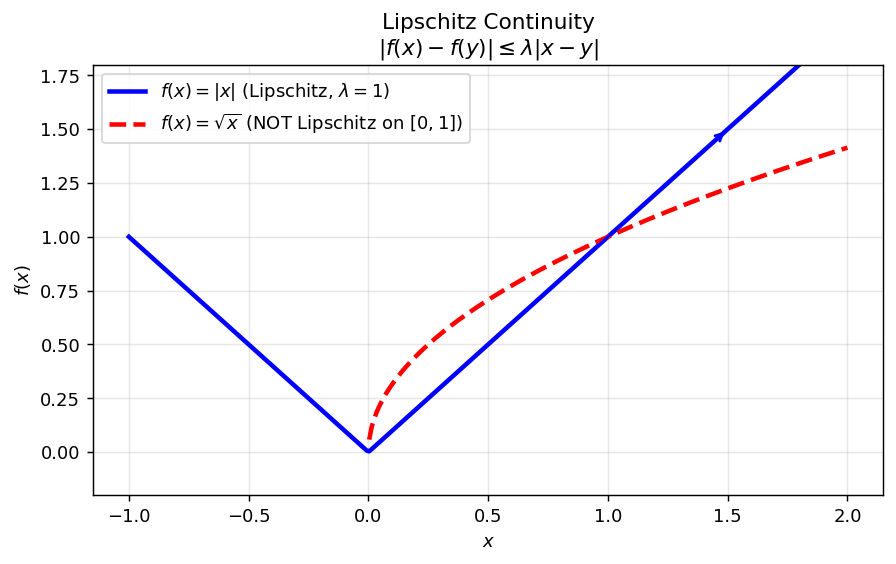Left: \(|x|\) is Lipschitz (chord slopes bounded). Right: \(\sqrt{x}\) on \([0,1]\) fails the condition near the origin.

Euler’s Method

To approximate the solution numerically, introduce a uniform time grid:

\[ t_0,\; t_1 = t_0 + h,\; t_2 = t_0 + 2h,\; \ldots \]

where \(h > 0\) is the time step. We seek numerical approximations \(y_n \approx \vec{y}(t_n)\).

The simplest method comes from integrating the ODE over one step:

\[ \vec{y}(t_{n+1}) = \vec{y}(t_n) + \int_{t_n}^{t_{n+1}} \vec{f}(t, \vec{y}(t))\, dt. \]

Replace the integrand by its value at the left endpoint: \(\vec{f}(t, \vec{y}(t)) \approx \vec{f}(t_n, \vec{y}(t_n))\). This gives

The method is explicit: each new value \(\vec{y}_{n+1}\) is computed directly from the known \(\vec{y}_n\) with no need to solve a nonlinear equation.

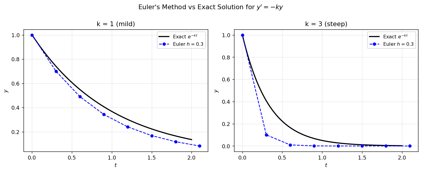Euler’s method (blue dashed) versus exact solution (black) for \(y' = -ky\), \(y(0)=1\). For mild decay (\(k=1\)) the method tracks well; for steep decay (\(k=3\)) the discrete steps overshoot more noticeably.

Convergence of Euler’s Method

The subscript \(h\) on \(\vec{y}_{n,h}\) emphasizes that the numerical solution depends on the step size. If a method does not converge, it is mathematically useless regardless of how cheap it is computationally.

The bound shows that the global error is \(O(h)\): halving the step size halves the error. Euler’s method is therefore a first-order method.

Local Truncation Error and Order

The order of a method characterises how accurately it approximates the ODE over a single step. Substituting the exact solution into Euler’s scheme:

\[ \vec{y}(t_{n+1}) - \big(\vec{y}(t_n) + h\vec{f}(t_n, \vec{y}(t_n))\big) = O(h^2). \]

This local error of \(O(h^2)\) means that per step the method makes an error of order \(h^2\); accumulated over \(O(1/h)\) steps, the global error is \(O(h)\).

The Trapezoidal Rule

Instead of approximating \(\vec{f}\) by its value at the left endpoint, we can use the average of its values at both endpoints:

This is an implicit method: \(\vec{y}_{n+1}\) appears on both sides of the equation. For linear problems this is no obstacle (rearrange and solve directly), but for nonlinear problems it requires iterative solvers (see Chapter 7).

Order of the trapezoidal rule. Substituting the exact solution and expanding by Taylor’s theorem:

\[ \vec{y}(t_{n+1}) - \vec{y}(t_n) - \frac{h}{2}\left[\vec{f}(t_n,\vec{y}(t_n)) + \vec{f}(t_{n+1},\vec{y}(t_{n+1}))\right] = O(h^3), \]

so the trapezoidal rule is second-order accurate. The convergence proof parallels that of Euler’s method but is more involved because of the implicit structure; the key estimate produces

\[ \|\vec{e}_{n+1,h}\| \leq \frac{c}{\lambda}\left[\left(\frac{1+\tfrac{1}{2}h\lambda}{1-\tfrac{1}{2}h\lambda}\right)^n - 1\right]h^2. \]

Since \(\frac{1+\tfrac{1}{2}h\lambda}{1-\tfrac{1}{2}h\lambda} \leq e^{h\lambda/(1-\tfrac{1}{2}h\lambda)}\), the global error is \(O(h^2)\).

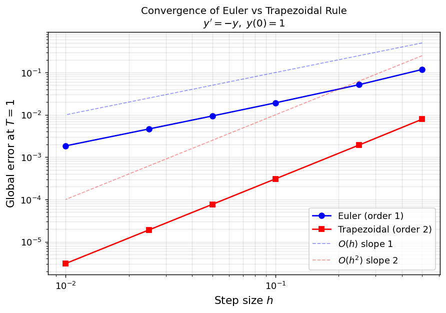Log–log plot of global error at \(T=1\) for \(y'=-y\). Euler’s error follows the \(O(h)\) reference line; the trapezoidal rule follows \(O(h^2)\). The trapezoidal rule achieves the same accuracy with far fewer time steps.

The \(\theta\)-Method Family

Both Euler’s method and the trapezoidal rule belong to a one-parameter family:

Special cases:

• \(\theta = 1\): Euler’s method (explicit, order 1).
• \(\theta = \tfrac{1}{2}\): Trapezoidal rule (implicit, order 2).
• \(\theta = 0\): Backward Euler or implicit Euler (implicit, order 1).

The order of the \(\theta\)-method is determined by substituting the exact solution. The local residual is

\[ \left(\theta - \tfrac{1}{2}\right)h^2\vec{y}''(t_n) + O(h^3). \]

This vanishes to second order only when \(\theta = \tfrac{1}{2}\); for all other \(\theta\) the method is first order. Backward Euler (\(\theta=0\)) sacrifices accuracy for superior stability properties that make it the method of choice for stiff problems (Chapter 4).

---

Chapter 2: Multistep Methods

From One-Step to Multistep

One-step methods use only the previous value \(\vec{y}_n\) to compute \(\vec{y}_{n+1}\). Multistep methods exploit the entire history of computed values \(\vec{y}_n, \vec{y}_{n-1}, \ldots, \vec{y}_{n-s+1}\) and corresponding slopes to achieve higher accuracy without the additional function evaluations required by Runge-Kutta.

The motivating observation is: if we have already evaluated \(\vec{f}\) at \(s\) past time points, a polynomial interpolant through these evaluations provides a much better approximation to \(\vec{f}(t,\vec{y}(t))\) than the constant used by Euler’s method.

Adams-Bashforth Methods

Integrate the ODE over one step:

\[ \vec{y}(t_{n+s}) = \vec{y}(t_{n+s-1}) + \int_{t_{n+s-1}}^{t_{n+s}} \vec{f}(t, \vec{y}(t))\, dt. \]

Fit a degree-\((s-1)\) polynomial \(\vec{p}(t)\) through the \(s\) past \(\vec{f}\)-values at \(t_{n}, t_{n+1}, \ldots, t_{n+s-1}\) using Lagrange interpolation:

\[ \vec{p}(t) = \sum_{m=0}^{s-1} p_m(t)\, \vec{f}(t_{n+m}, \vec{y}_{n+m}), \qquad p_m(t_{n+k}) = \begin{cases} 1 & k = m \\ 0 & k \neq m. \end{cases} \]

Defining \(b_m = \frac{1}{h}\int_{t_{n+s-1}}^{t_{n+s}} p_m(t)\, dt\) yields the Adams-Bashforth family:

\[ \vec{y}_{n+s} = \vec{y}_{n+s-1} + h\sum_{m=0}^{s-1} b_m\, \vec{f}(t_{n+m}, \vec{y}_{n+m}). \]

These methods are explicit (no \(\vec{f}(t_{n+s}, \vec{y}_{n+s})\) appears) and of order \(s\).

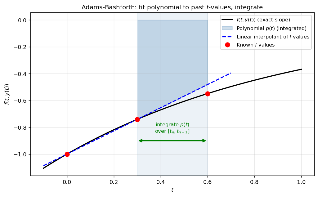The 2-step Adams-Bashforth method fits a linear polynomial through the two most recent \(f\)-values (red dots) and integrates it over the next interval (shaded). This provides a better approximation than Euler’s constant extrapolation.

The 2-step Adams-Bashforth method has weights \(b_0 = -\tfrac{1}{2}\), \(b_1 = \tfrac{3}{2}\):

\[ \vec{y}_{n+2} = \vec{y}_{n+1} + h\left(-\tfrac{1}{2}\vec{f}(t_n,\vec{y}_n) + \tfrac{3}{2}\vec{f}(t_{n+1},\vec{y}_{n+1})\right). \]

The 1-step member is exactly Euler’s method. Halving \(h\) in an \(s\)-step Adams-Bashforth method reduces the global error by a factor of \(2^s\), which is a powerful acceleration.

Adams-Moulton Methods

Extending the polynomial to include the unknown endpoint \(t_{n+s}\) produces implicit methods known as Adams-Moulton methods. By including one extra interpolation point, the order increases by one: an \(s\)-step Adams-Moulton method achieves order \(s+1\). The 2-step Adams-Moulton method (also called the implicit trapezoidal corrector) has weights \(b_0 = -\tfrac{1}{12}, b_1 = \tfrac{2}{3}, b_2 = \tfrac{5}{12}\):

\[ \vec{y}_{n+2} = \vec{y}_{n+1} + h\left(-\tfrac{1}{12}\vec{f}(t_n,\vec{y}_n) + \tfrac{2}{3}\vec{f}(t_{n+1},\vec{y}_{n+1}) + \tfrac{5}{12}\vec{f}(t_{n+2},\vec{y}_{n+2})\right). \]

In practice, Adams-Bashforth and Adams-Moulton methods are paired as predictor-corrector schemes: the explicit AB step provides a cheap first guess, which the implicit AM step refines.

General Linear Multistep Methods and Their Order

The general \(s\)-step linear multistep method takes the form

\[ \sum_{m=0}^{s} a_m\, \vec{y}_{n+m} = h\sum_{m=0}^{s} b_m\, \vec{f}(t_{n+m},\vec{y}_{n+m}), \quad n = 0, 1, 2, \ldots \]

with constants \(a_m, b_m\) independent of \(h\) and \(n\). If \(b_s = 0\) the method is explicit; if \(b_s \neq 0\) it is implicit. Define the characteristic polynomials:

\[ \rho(\omega) = \sum_{m=0}^{s} a_m\, \omega^m, \qquad \sigma(\omega) = \sum_{m=0}^{s} b_m\, \omega^m. \]

Equivalently, the conditions \(\sum_m a_m = 0\) and \(\sum_m m^k a_m = k\sum_m m^{k-1} b_m\) for \(k = 1, \ldots, p\) must hold, with strict inequality for \(k = p+1\).

Convergence: The Dahlquist Equivalence Theorem

For multistep methods, convergence requires two ingredients: the local truncation error must vanish (consistency), and the method must not amplify parasitic solution components (zero-stability).

The root condition is the multistep analogue of a stability criterion. To see why it matters, consider the method with \(\rho(\omega) = \omega^2 - 3\omega + 2 = (\omega-1)(\omega-2)\). This has a root \(\omega = 2\) outside the unit disk. Even though it may be consistent, the \(\omega=2\) root generates a spurious mode that grows as \(2^n\), overwhelming the physical solution.

Adams-Bashforth methods use \(\rho(\omega) = \omega^{s-1}(\omega - 1)\), which has roots \(\omega = 1\) (simple) and \(\omega = 0\) (with multiplicity \(s-1\), inside the unit disk). They satisfy the root condition for all \(s \geq 1\).

Backward Differentiation Formulae (BDF)

Setting \(\sigma(\omega) = \beta\omega^s\) (only the most recent function value appears) leads to the Backward Differentiation Formula family. The BDF methods differentiate a polynomial interpolant and set it equal to \(\vec{f}\) at the current point. For \(s = 1\), BDF-1 is Backward Euler:

\[ \vec{y}_{n+1} = \vec{y}_n + h\,\vec{f}(t_{n+1}, \vec{y}_{n+1}). \]

The \(\rho\) polynomial for the BDF-\(s\) method is:

\[ \rho(\omega) = \beta\sum_{m=1}^{s} \frac{1}{m}\,\omega^{s-m}(\omega-1)^m, \]

chosen so that \(a_s = 1\). BDF methods are implicit, achieve order \(s\), and satisfy the root condition for \(s \leq 6\). They are the dominant choice for stiff problems in computational practice.

Constructing Multistep Methods Systematically

Given a desired \(\rho\) (step 1), one recovers the optimal \(\sigma\) from the order conditions by expanding \(\rho(\omega)/\ln(\omega)\) around \(\omega = 1\) and truncating. Explicit methods truncate after the degree-\((s-1)\) term; implicit methods include the degree-\(s\) term for one extra order.

The maximum achievable order of an \(s\)-step method is:

\[ p \leq \begin{cases} s+1 & \text{implicit} \\ s & \text{explicit.} \end{cases} \]

---

Chapter 3: Runge-Kutta Methods

The Idea: Quadrature Plus Internal Stages

Multistep methods gain accuracy by reusing past function evaluations. Runge-Kutta methods gain accuracy by evaluating \(\vec{f}\) at several intermediate points within a single step—no history needed.

Integrating the IVP over one step:

\[ \vec{y}(t_{n+1}) = \vec{y}(t_n) + h\int_0^1 \vec{f}(t_n + h\tau,\, \vec{y}(t_n+h\tau))\, d\tau. \]

Approximate the integral by a quadrature rule with nodes \(c_j \in [0,1]\) and weights \(b_j > 0\):

\[ \int_0^1 \vec{f}(t_n + h\tau, \vec{y}(t_n+h\tau))\, d\tau \approx \sum_{j=1}^{\nu} b_j\, \vec{f}(t_n + c_j h,\, \vec{y}(t_n+c_jh)). \]

The values \(\vec{y}(t_n + c_j h)\) are unknown, so we build them up iteratively as internal stages \(\vec{k}_j\):

\[ \vec{k}_j = \vec{y}_n + h\sum_{i=1}^{j-1} a_{j,i}\, \vec{f}(t_n + c_i h, \vec{k}_i), \qquad j = 1, 2, \ldots, \nu. \]

The update then reads:

\[ \vec{y}_{n+1} = \vec{y}_n + h\sum_{j=1}^{\nu} b_j\, \vec{f}(t_n + c_j h, \vec{k}_j). \]

Gaussian Quadrature

The choice of nodes \(c_j\) determines the order of the quadrature, and hence the order of the resulting Runge-Kutta method. To maximise the order of integration for a fixed number of nodes \(\nu\), we use Gaussian quadrature.

The Vandermonde system that determines the weights is nonsingular whenever the nodes are distinct. With a free choice of nodes (not prescribed), one can double the order: the Gauss-Legendre nodes are the zeros of the degree-\(\nu\) Legendre polynomial. To use these as quadrature nodes, we need to know that degree-\(\nu\) orthogonal polynomials have exactly \(\nu\) distinct real zeros inside \((a,b)\).

With the GL nodes guaranteeing \(\nu\) distinct nodes in \((0,1)\), Lemma 3.1 applies and the formula integrates polynomials of degree up to \(2\nu-1\) exactly. This is the best possible for any \(\nu\)-point formula.

The bound in Theorem 3.1 is tight in both directions: the GL formula achieves order exactly \(2\nu\). The achievability follows from an orthogonality argument; the impossibility of order \(2\nu+1\) follows from a direct counter-example.

The orthogonality argument in this proof generalises to yield a sharp characterisation of when any quadrature formula exceeds its baseline order.

In other words, the formula gains \(m\) bonus orders of accuracy precisely when the nodal polynomial is orthogonal to all polynomials of degree \(\leq m-1\). The GL nodes maximise this: by construction, \(\omega = \hat{P}_\nu\) is orthogonal to all polynomials of degree \(\leq \nu - 1\), yielding \(m = \nu\) and total order \(2\nu\). Theorem 3.4 is the key to extending the analysis from quadrature to collocation methods in §3.4.

Explicit Runge-Kutta Methods and Butcher Tableaux

When the matrix \(A = (a_{j,i})\) is strictly lower-triangular, the stages \(\vec{k}_j\) are computed sequentially without solving any linear system. This is an explicit Runge-Kutta (ERK) method. The structure of an ERK method is encoded in its Butcher tableau:

\[ \begin{array}{c|ccc} c_1 & 0 & & \\ c_2 & a_{2,1} & 0 & \\ \vdots & \vdots & \ddots & \\ c_\nu & a_{\nu,1} & \cdots & 0 \\ \hline & b_1 & \cdots & b_\nu \end{array} \]

For a 2-stage ERK to achieve order \(p \geq 2\), the parameters must satisfy:

\[ b_1 + b_2 = 1, \qquad b_2 c_2 = \tfrac{1}{2}, \qquad a_{2,1} = c_2. \]

These three conditions have a family of solutions; popular choices include:

• \(b_1 = 0,\, b_2 = 1,\, c_2 = \tfrac{1}{2}\): the midpoint rule (or modified Euler).
• \(b_1 = b_2 = \tfrac{1}{2},\, c_2 = 1\): the Heun method.

For a 3-stage ERK of order 3, there are four order conditions, and for the celebrated 4-stage RK4 method of order 4:

\[ \begin{array}{c|cccc} 0 & & & & \\ \tfrac{1}{2} & \tfrac{1}{2} & & & \\ \tfrac{1}{2} & 0 & \tfrac{1}{2} & & \\ 1 & 0 & 0 & 1 & \\ \hline & \tfrac{1}{6} & \tfrac{1}{3} & \tfrac{1}{3} & \tfrac{1}{6} \end{array} \]

RK4 computes four slopes per step, combining them as a weighted average analogous to Simpson’s rule. It remains the default workhorse of scientific computing.

Implicit Runge-Kutta Methods

When \(A\) is not lower-triangular, the stage equations are coupled: all \(\nu\) stages must be solved simultaneously. These implicit Runge-Kutta (IRK) methods require solving a \(\nu d\)-dimensional nonlinear system per step, but they can achieve far superior stability properties.

The Gauss-Legendre IRK method of order \(2\nu\) uses Gauss-Legendre nodes and is \(A\)-stable for all \(\nu\) (see Chapter 4). For example, the 2-stage Gauss-Legendre method (the implicit midpoint rule variant) uses nodes \(c_{1,2} = \tfrac{1}{2} \mp \tfrac{\sqrt{3}}{6}\) and achieves order 4.

Connecting back to one-step methods: The 1-stage IRK with \(c_1 = \tfrac{1}{2}\), \(b_1 = 1\), \(a_{1,1} = \tfrac{1}{2}\) is the implicit midpoint rule; the 1-stage IRK with \(c_1 = 1\), \(b_1 = 1\), \(a_{1,1} = 1\) is Backward Euler.

Collocation Methods

Collocation provides an elegant reformulation of Runge-Kutta methods that connects them directly to polynomial approximation theory and makes the order properties proved in §3.1 immediately applicable.

The construction is explicit in structure even though it leads to implicit equations: since \(u'\) is a degree-\((\nu-1)\) polynomial satisfying \(\nu\) pointwise ODE conditions, Lagrange interpolation uniquely determines it. Integrating from \(t_n\) with the initial condition \(u(t_n) = \vec{y}_n\) then gives \(u\) itself. The stage values \(\vec{k}_j = u(t_n + c_j h)\) are the unknowns to be solved for.

The fundamental structural result is that collocation and IRK are not merely analogous — they are the same.

Defect, Error, and Order

Having identified collocation with IRK, we now analyse accuracy. Two quantities describe how well the collocation polynomial \(u\) approximates the true solution \(\vec{y}\).

The defect is the residual when \(u\) is plugged into the ODE; the error is the actual distance from the truth. The two are related through the variation-of-constants formula.

The theorem tells us: to bound the error, bound the defect. Since the defect vanishes at the \(\nu\) collocation nodes, it is small everywhere — and the size depends on how many additional orthogonality conditions the nodes satisfy.

This is the collocation analogue of Theorem 3.4: the orthogonality of the nodal polynomial against the first \(m\) monomials buys \(m\) extra orders. Choosing the GL nodes makes \(\omega = \hat{P}_\nu\) orthogonal to all polynomials of degree \(\leq \nu - 1\), giving \(m = \nu\) and total order \(2\nu\).

Gauss-Legendre Runge-Kutta

The \(\nu\)-stage Gauss-Legendre Runge-Kutta (GLRK) method is the collocation method with nodes equal to the zeros of the shifted Legendre polynomial \(\hat{P}_\nu\). Its coefficients are computed via Lemma 3.5, and by Theorem 3.7 it has order \(2\nu\).

1-stage GLRK (order 2, the implicit midpoint rule):

\[ \begin{array}{c|c} \tfrac{1}{2} & \tfrac{1}{2} \\[2pt] \hline & 1 \end{array} \]

2-stage GLRK (order 4): nodes \(c_{1,2} = \tfrac{1}{2} \mp \tfrac{\sqrt{3}}{6}\), weights \(b_1 = b_2 = \tfrac{1}{2}\):

\[ \begin{array}{c|cc} \tfrac{1}{2} - \tfrac{\sqrt{3}}{6} & \tfrac{1}{4} & \tfrac{1}{4} - \tfrac{\sqrt{3}}{6} \\[6pt] \tfrac{1}{2} + \tfrac{\sqrt{3}}{6} & \tfrac{1}{4} + \tfrac{\sqrt{3}}{6} & \tfrac{1}{4} \\[2pt] \hline & \tfrac{1}{2} & \tfrac{1}{2} \end{array} \]

The 2-stage GLRK method achieves order 4 with only 2 stages, and — as we prove in Chapter 4 — is A-stable. This combination of high order and unconditional stability makes it one of the most powerful methods in the course.

---

Chapter 4: Stiffness and Stability

Stiff Ordinary Differential Equations

Not all ODEs are equally amenable to numerical treatment. A stiff problem is one in which the exact solution decays on a moderate timescale, but the system contains fast transient modes that force explicit methods to take extremely small steps even when the mode being resolved decays slowly.

A prototypical example is the linear system \(\vec{y}' = N\vec{y}\) with

\[ N = \begin{bmatrix} -100 & 1 \\ 0 & -10 \end{bmatrix}. \]

The eigenvalues are \(\lambda_1 = -100\) and \(\lambda_2 = -10\). Both components decay to zero (the problem is numerically easy in terms of the long-time solution), but the fastest mode has \(|Re(\lambda_1)| = 100\), which will force Euler’s method to take steps \(h < 1/50\) just to remain stable—far smaller than needed for accuracy.

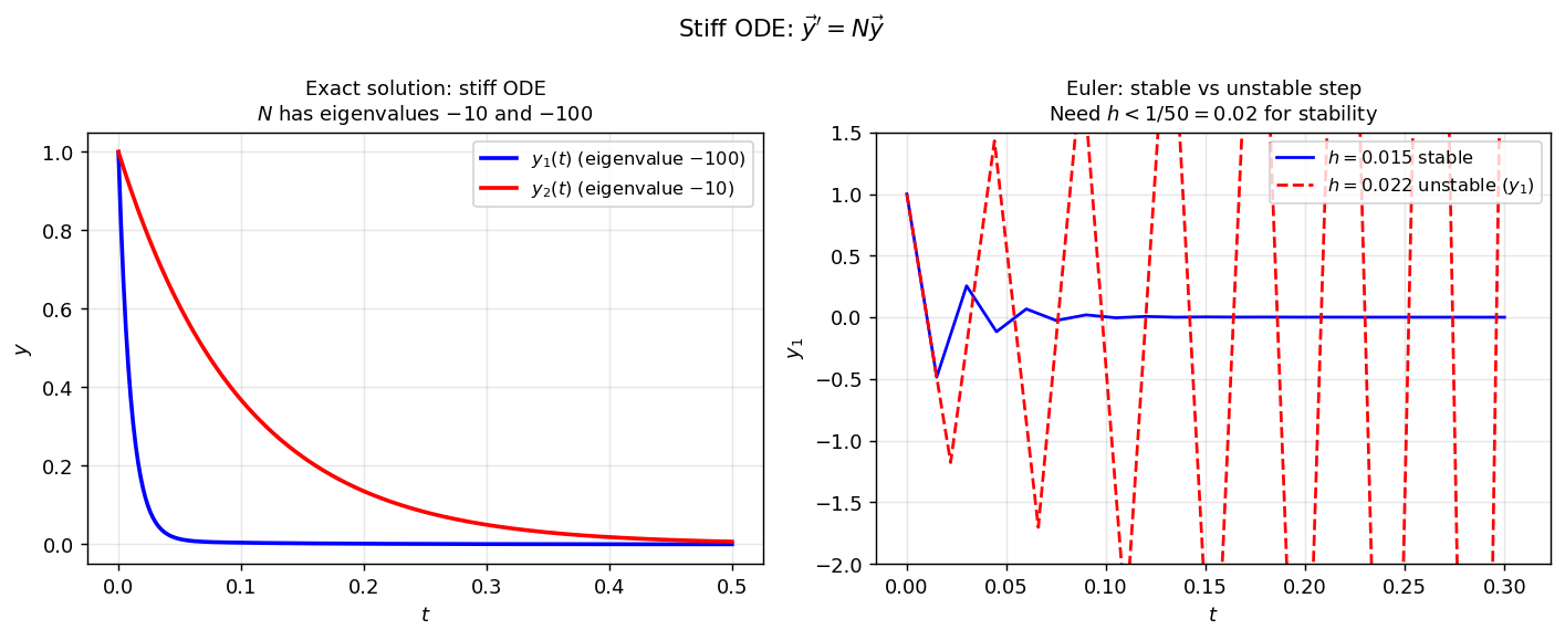Left: exact solution of the stiff system—both components decay, with \(y_1\) (linked to eigenvalue \(-100\)) decaying much faster. Right: Euler’s method with \(h = 0.015\) stays stable, while \(h = 0.022 > 1/50\) produces wild oscillations in \(y_1\).

Spectral Decomposition and the Step Size Constraint

To make the stiffness constraint precise, solve the system exactly via spectral decomposition. Factor \(N = VDV^{-1}\) where \(D = \mathrm{diag}(\lambda_1, \lambda_2) = \mathrm{diag}(-100, -10)\) and \(V\) contains the corresponding eigenvectors. The exact solution is then

\[ \vec{y}(t) = V e^{tD} V^{-1} \vec{y}_0 = V \begin{bmatrix} e^{-100t} & 0 \\ 0 & e^{-10t} \end{bmatrix} V^{-1} \vec{y}_0. \]

Euler’s method gives \(\vec{y}_{n+1} = (I + hN)\vec{y}_n\), so by induction \(\vec{y}_n = (I + hN)^n \vec{y}_0 = V(I + hD)^n V^{-1} \vec{y}_0\). For the numerical solution to decay, each diagonal entry of \((I + hD)\) must satisfy \(|1 + h\lambda_j| < 1\), which requires \(-2 < h\lambda_j < 0\), i.e., \(h < 2/|\lambda_j|\). Checking both eigenvalues:

\[ h < \frac{2}{100} = \frac{1}{50} \qquad \text{and} \qquad h < \frac{2}{10} = \frac{1}{5}. \]

The binding constraint is \(h < 1/50\), imposed by the fast mode \(e^{-100t}\). Yet that mode has essentially vanished for \(t \gtrsim 0.05\). We are compelled to use tiny time steps for a transient that is irrelevant on the timescale of interest — the defining pathology of stiffness. The stiffness ratio \(|\lambda_{\max}|/|\lambda_{\min}| = 10\) quantifies the severity; ratios of \(10^6\) or more are common in chemical kinetics and structural dynamics.

Linear Stability Domain

To analyse stability, focus on the linear scalar test equation:

\[ y' = \lambda y, \quad y(0) = 1, \quad \lambda \in \mathbb{C}, \quad \text{Re}(\lambda) < 0. \]

The exact solution \(y(t) = e^{\lambda t} \to 0\) as \(t \to \infty\).

Euler’s method gives \(y_{n+1} = (1 + h\lambda)y_n = (1+z)y_n\), so \(y_n = (1+z)^n \to 0\) if and only if \(|1+z| < 1\). The stability domain is the disk of radius 1 centred at \(-1\):

\[ D_{\text{Euler}} = \{z \in \mathbb{C} : |1+z| < 1\}. \]

Trapezoidal rule gives \(y_{n+1} = \frac{1+\tfrac{1}{2}z}{1-\tfrac{1}{2}z}\, y_n\). Since \(|{(1+\tfrac{1}{2}z)}/{(1-\tfrac{1}{2}z)}| < 1\) precisely when \(\text{Re}(z) < 0\), the stability domain is the entire left half-plane:

\[ D_{\text{Trap}} = \{z \in \mathbb{C} : \text{Re}(z) < 0\}. \]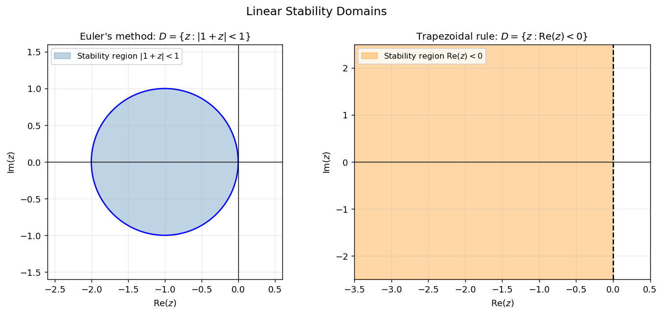

Left: Euler’s stability region — a disk of radius 1 centred at \(-1\). For the stiff system above, we need \(h|\lambda_1| \leq 2\), i.e., \(h \leq 0.02\). Right: Trapezoidal rule — the entire left half-plane. Any step size works as long as \(\text{Re}(h\lambda) < 0\).

A-Stability

A-stability means the method remains stable for any step size applied to any decaying problem—the method cannot be destabilised by reducing the step size would only help. The trapezoidal rule is A-stable; Euler’s method is not.

This follows because the stability function \(r(z)\) of an explicit RK method is a polynomial, and a polynomial satisfying \(|r(z)| < 1\) for all \(\text{Re}(z) < 0\) would have to be bounded by 1 on the closed left half-plane while satisfying \(r(0) = 1\)—which the maximum principle prevents.

A-Stability of Runge-Kutta Methods

For any Runge-Kutta method applied to \(y' = \lambda y\), the numerical solution after one step satisfies \(y_{n+1} = r(h\lambda)\, y_n\) where the stability function \(r \in P_{\nu\nu}\) (rational functions of degree at most \(\nu\) in both numerator and denominator) is given by:

\[ r(z) = 1 + z\, \vec{b}^T (I - zA)^{-1} \vec{1}. \]

The linear stability domain can then be expressed directly in terms of \(r\).

The proof is immediate from the recurrence \(y_{n+1} = r(h\lambda)\,y_n\). The stability domain is the preimage of the open unit disk under \(r\). For explicit methods, since \(r\) is a polynomial of bounded degree, \(D\) is always bounded — confirming that no explicit method can be A-stable.

For explicit RK, \(A\) is strictly lower-triangular so \(\det(I - zA) = 1\) and \(r\) is a polynomial.

Padé Approximation and Gauss-Legendre IRK

The link between method order and the stability function is made precise by the following lemma.

This says that among all rational functions in \(\mathcal{P}_{\alpha\beta}\), the stability function of a high-order method is the one that best approximates \(e^z\) near the origin. The classical theory of Padé approximation provides exactly such approximants.

Key instances:

• \(\hat{f}_{10}(z) = 1 + z\) — Euler’s method (stability function of the 1-stage explicit RK of order 1).
• \(\hat{f}_{11}(z) = (1 + \tfrac{1}{2}z)/(1 - \tfrac{1}{2}z)\) — the trapezoidal rule (1-stage GLRK).
• \(\hat{f}_{22}(z)\) — stability function of the 2-stage GLRK method of order 4.

The stability function of a \(p\)-th order method satisfies \(r(z) = e^z + O(z^{p+1})\). The Padé approximant \(\hat{f}_{\alpha\beta}\) is the unique rational function in \(P_{\alpha\beta}\) of order \(\alpha+\beta\):

\[ \hat{p}_{\alpha\beta}(z) = \sum_{k=0}^\alpha \binom{\alpha}{k}\frac{(\alpha+\beta-k)!}{(\alpha+\beta)!} z^k, \qquad \hat{q}_{\alpha\beta}(z) = \hat{p}_{\beta\alpha}(-z). \]

The Gauss-Legendre IRK method of \(\nu\) stages has stability function \(r = \hat{f}_{\nu\nu}\), the diagonal Padé approximant to \(e^z\). The final step to A-stability is:

The proof (omitted) uses Lemma 4.3: one checks that all poles of \(\hat{f}_{\alpha\beta}\) have positive real part, and then verifies \(|\hat{f}_{\alpha\beta}(it)| \leq 1\) for all \(t \in \mathbb{R}\) by a direct computation in polar coordinates.

Combining the results: the \(\nu\)-stage GLRK method has order \(2\nu\) (§3.4), so by Lemma 4.4 its stability function satisfies \(r(z) = e^z + O(z^{2\nu+1})\), and by Theorem 4.5 this forces \(r = \hat{f}_{\nu\nu}\). Since \(\alpha = \beta = \nu\) satisfies \(\alpha \leq \beta \leq \alpha + 2\), Theorem 4.6 gives A-stability. This chain of reasoning shows all Gauss-Legendre IRK methods are A-stable for every \(\nu \geq 1\) — a fundamental reason they dominate in stiff computations.

The trapezoidal rule is exactly the 1-stage Gauss-Legendre method with \(r(z) = \hat{f}_{11}(z) = \frac{1+\tfrac{1}{2}z}{1-\tfrac{1}{2}z}\).

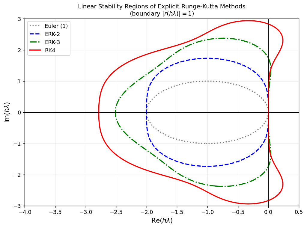Stability region boundaries \(|r(h\lambda)|=1\) for explicit RK methods of orders 1–4. As the order increases the region grows, but all ERK methods have bounded stability domains. IRK methods (not shown) can cover the entire left half-plane.

---

Chapter 5: Numerical Methods for PDEs

Classification of Second-Order PDEs

The transition from ODEs to PDEs introduces a new complexity: the qualitative behaviour of solutions—and the appropriate numerical treatment—depends critically on the type of the equation. A general second-order PDE in two variables has the form

\[ A(x,y)\,\partial_{xx}u + B(x,y)\,\partial_{xy}u + C(x,y)\,\partial_{yy}u = w(u, \partial_x u, \partial_y u, x, y). \]

The discriminant \(B^2 - 4AC\) classifies the PDE:

• Parabolic if \(B^2 - 4AC = 0\) (e.g., heat equation).
• Hyperbolic if \(B^2 - 4AC > 0\) (e.g., wave equation).
• Elliptic if \(B^2 - 4AC < 0\) (e.g., Laplace’s equation).

This course focuses on the parabolic case; the methods and theory extend naturally.

The Heat Equation

The model parabolic PDE is the heat equation:

\[ \begin{cases} \partial_t u = \partial_{xx} u, & t > 0,\; 0 < x < 1, \\ u(0,t) = u(1,t) = 0, & t \geq 0, \\ u(x,0) = u_0(x), & 0 \leq x \leq 1. \end{cases} \]

Here \(u(x,t)\) represents temperature, \(x\) is position, and \(t\) is time. The zero Dirichlet boundary conditions model a rod with endpoints held at temperature zero.

The diffusion operator \(\partial_{xx}\) smooths out initial oscillations: high-frequency modes decay fast, low-frequency modes persist. The exact solution via separation of variables is:

\[ u(x,t) = \sum_{m=1}^\infty a_m \sin(m\pi x)\, e^{-(m\pi)^2 t}, \]

where \(a_m = 2\int_0^1 u_0(x)\sin(m\pi x)\, dx\) are the Fourier sine coefficients of the initial data. The mode \(m\) decays at rate \((m\pi)^2\), so high-frequency components vanish rapidly.

Finite Difference Discretization

Step 1: Spatial grid. Partition \([0,1]\) into \(J\) uniform intervals of width \(\Delta x = 1/J\), giving nodes \(x_j = j\Delta x\) for \(j = 0, 1, \ldots, J\).

Step 2: Time grid. Use uniform time steps \(\Delta t\), giving \(t_n = n\Delta t\).

Step 3: Replace derivatives by finite differences. Taylor’s theorem gives:

\[ \frac{\partial u}{\partial t}(x_j, t_n) \approx \frac{u(x_j, t_n + \Delta t) - u(x_j, t_n)}{\Delta t} + O(\Delta t) \quad \text{(forward difference)}, \]\[ \frac{\partial^2 u}{\partial x^2}(x_j, t_n) \approx \frac{u(x_j+\Delta x, t_n) - 2u(x_j,t_n) + u(x_j-\Delta x,t_n)}{(\Delta x)^2} + O((\Delta x)^2) \quad \text{(central difference)}. \]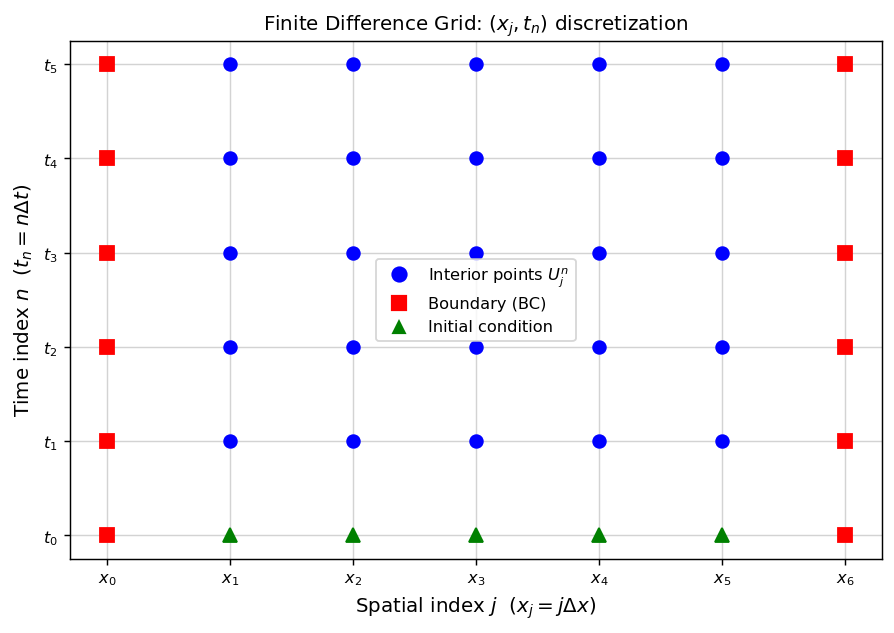

The discretization domain: interior points (blue circles) are solved for; boundary points (red squares) are determined by Dirichlet conditions; the bottom row (green triangles) is set by the initial condition.

Substituting into the PDE gives the explicit (forward Euler) finite difference scheme. Let \(U_j^n\) denote the numerical approximation to \(u(x_j, t_n)\):

\[ \frac{U_j^{n+1} - U_j^n}{\Delta t} = \frac{U_{j+1}^n - 2U_j^n + U_{j-1}^n}{(\Delta x)^2}, \quad j = 1, \ldots, J-1. \]

Introducing the mesh ratio \(\nu = \Delta t / (\Delta x)^2\), this becomes:

\[ U_j^{n+1} = U_j^n + \nu\left(U_{j+1}^n - 2U_j^n + U_{j-1}^n\right) = (1-2\nu)U_j^n + \nu U_{j+1}^n + \nu U_{j-1}^n. \]

Truncation Error and Consistency

The truncation error \(T(x,t)\) is what remains when the exact solution is substituted into the finite difference scheme:

\[ T(x_j, t_n) = \frac{u(x_j, t_n+\Delta t) - u(x_j, t_n)}{\Delta t} - \frac{u(x_j+\Delta x, t_n) - 2u(x_j,t_n) + u(x_j-\Delta x,t_n)}{(\Delta x)^2}. \]

Expanding by Taylor’s theorem:

\[ T(x,t) = \frac{1}{2}\Delta t\, u_{tt} + O(\Delta t^2) - \frac{1}{12}(\Delta x)^2 u_{xxxx} + O((\Delta x)^4). \]

Since \(u_t = u_{xx}\) (the PDE), we can substitute \(u_{tt} = u_{xxxt}\). The truncation error is \(O(\Delta t) + O((\Delta x)^2)\). The scheme is:

• First-order accurate in time and second-order accurate in space.
• Consistent: \(T \to 0\) as \(\Delta t, \Delta x \to 0\) independently.

If we fix the ratio \(\nu = \Delta t/(\Delta x)^2\), then \(\Delta t = \nu(\Delta x)^2\) and the leading term in \(T\) becomes \(\frac{\nu}{2}(\Delta x)^2 u_{xxxx}\), making the overall error \(O((\Delta x)^2)\) on a fixed refinement path.

Increasing accuracy via modified equation: Using the relation \(u_{tt} = u_{xxxt}\), the truncation error can be written as \(\frac{1}{2}\Delta t(1 - \frac{1}{6\nu})u_{xxxx} + O(\Delta t^2)\). Choosing \(\nu = 1/6\) eliminates the leading error term, giving an effectively second-order method in time along this special path.

Von Neumann Stability Analysis

A scheme is stable if rounding errors do not grow unboundedly. For a linear PDE with constant coefficients, we test stability by inserting a Fourier mode ansatz:

\[ U_j^n = \lambda^n e^{ijk\Delta x}. \]

Substituting into the forward-Euler FD scheme:

\[ \lambda = 1 + \nu(e^{ik\Delta x} - 2 + e^{-ik\Delta x}) = 1 - 4\nu\sin^2\!\left(\tfrac{k\Delta x}{2}\right). \]

The amplification factor is \(\lambda(k) = 1 - 4\nu\sin^2(k\Delta x/2)\). For stability, all modes must not grow: \(|\lambda(k)| \leq 1\) for all \(k\).

This CFL condition (Courant-Friedrichs-Lewy) states that we cannot take arbitrarily large time steps—the time step must scale as \((\Delta x)^2\). This is a severe restriction: halving the spatial step forces a quartering of the time step and an eightfold increase in total computational work.

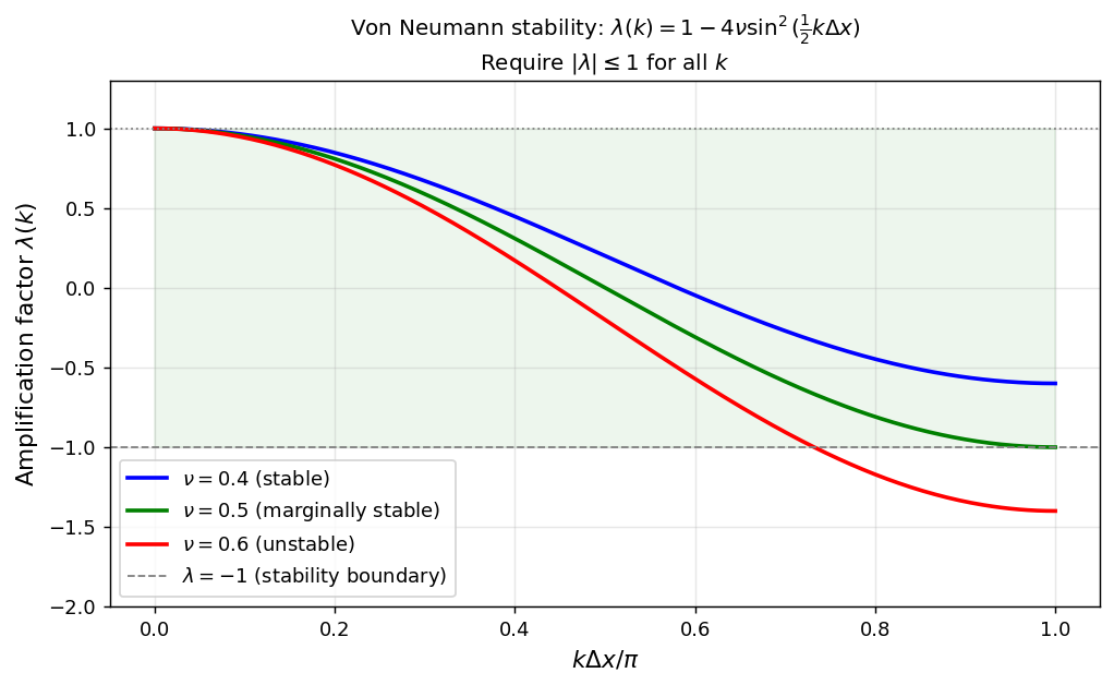Amplification factor \(\lambda(k)\) as a function of wavenumber. For \(\nu = 0.4 \leq 1/2\) (blue), \(|\lambda| \leq 1\) for all \(k\). For \(\nu = 0.6 > 1/2\) (red), high-frequency modes have \(\lambda < -1\) and grow without bound.

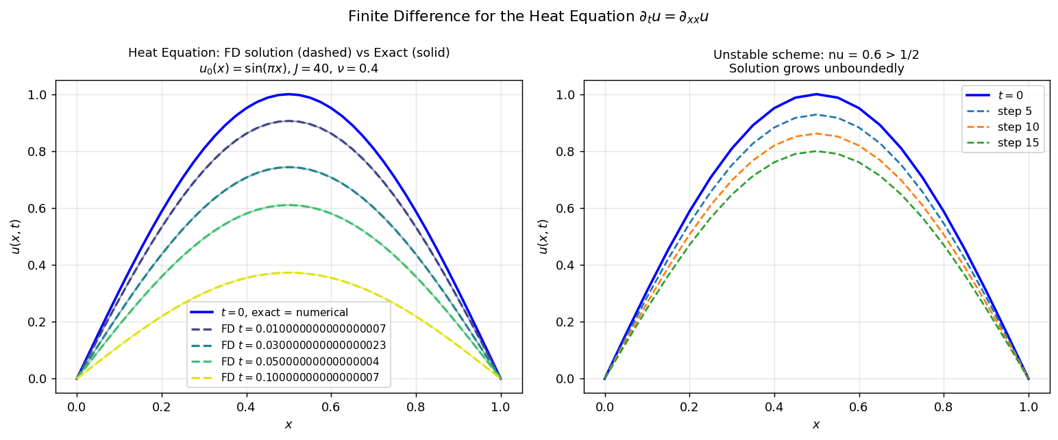Left: stable forward-Euler scheme (\(\nu=0.4\)) tracking the exact solution (solid) closely at multiple time snapshots. Right: unstable scheme (\(\nu=0.6\)) — the high-frequency modes amplify and destroy the solution.

Convergence and the Lax Equivalence Theorem

Define the error \(e_j^n = U_j^n - u(x_j, t_n)\). Subtracting the exact equation from the FD equation:

\[ e_j^{n+1} = (1-2\nu)e_j^n + \nu e_{j+1}^n + \nu e_{j-1}^n - \Delta t\, T(x_j, t_n). \]

Setting \(E^n = \max_j |e_j^n|\) and assuming \(\nu \leq \tfrac{1}{2}\) (so all coefficients are non-negative):

\[ E^{n+1} \leq E^n + \Delta t \cdot C\Delta t = E^n + C(\Delta t)^2. \]

Since \(E^0 = 0\), we have \(E^n \leq nC(\Delta t)^2 \leq T_F \cdot C\Delta t \to 0\) as \(\Delta t \to 0\). The method is convergent.

This relationship between consistency, stability, and convergence is the content of the fundamental result in numerical PDE:

The \(\theta\)-Method for the Heat Equation

The implicit equivalent applies the \(\theta\)-method in time while keeping the central difference in space:

\[ \frac{U_j^{n+1} - U_j^n}{\Delta t} = \theta\, \frac{U_{j+1}^{n+1} - 2U_j^{n+1} + U_{j-1}^{n+1}}{(\Delta x)^2} + (1-\theta)\, \frac{U_{j+1}^n - 2U_j^n + U_{j-1}^n}{(\Delta x)^2}. \]

• \(\theta = 0\): Forward Euler (explicit, first-order in time, stable iff \(\nu \leq 1/2\)).
• \(\theta = \tfrac{1}{2}\): Crank-Nicolson (implicit, second-order in time, unconditionally stable).
• \(\theta = 1\): Backward Euler (implicit, first-order in time, unconditionally stable).

Maximum Principle and Convergence of the \(\theta\)-Method

Convergence of the general \(\theta\)-method follows from a maximum principle: the solution of the heat equation cannot exceed the maximum of its initial and boundary data. The discrete analogue holds for the \(\theta\)-method under a mild condition.

The maximum principle gives the convergence proof directly:

Summary of \(\theta\)-method properties:

\(\theta\)	Order in time	Stability condition	Explicit/implicit
\(0\)	\(O(\Delta t)\)	\(\nu \leq \tfrac{1}{2}\)	Explicit
\(\tfrac{1}{2}\)	\(O(\Delta t^2)\)	Unconditional	Implicit
\(1\)	\(O(\Delta t)\)	Unconditional	Implicit

Crank-Nicolson is the workhorse of PDE time integration: it achieves second-order accuracy in both space and time while imposing no stability restriction on \(\nu\). The implicit system at each time step is tridiagonal and can be solved in \(O(J)\) operations by the Thomas algorithm below.

Stability of Backward Euler for the Heat Equation

For the backward Euler scheme (\(\theta = 1\)), inserting the von Neumann ansatz \(U_j^n = \lambda^n e^{ijk\Delta x}\) gives

\[ \lambda = 1 + \nu\lambda(e^{ik\Delta x} - 2 + e^{-ik\Delta x}) = 1 - 4\nu\lambda\sin^2\!\left(\tfrac{k\Delta x}{2}\right). \]

Solving for \(\lambda\):

\[ \lambda(k) = \frac{1}{1 + 4\nu\sin^2\!\left(\tfrac{k\Delta x}{2}\right)}. \]

Since \(4\nu\sin^2(\cdot) \geq 0\), the denominator is always \(\geq 1\), so \(0 < \lambda(k) \leq 1\) for all \(k\) and all \(\nu > 0\). Backward Euler is therefore unconditionally stable: no CFL restriction on the mesh ratio. The price is a tridiagonal linear system to solve at each time step, but with the Thomas algorithm this costs only \(O(J)\) operations.

The Thomas Algorithm

At each time step of an implicit finite difference scheme, we must solve a tridiagonal linear system:

\[ a_k U_{k-1} + b_k U_k + c_k U_{k+1} = d_k, \qquad k = 1, 2, \ldots, J-1, \]

with \(U_0 = U_J = 0\) from the boundary conditions. The Thomas algorithm solves this in \(O(J)\) operations by Gaussian elimination adapted to the tridiagonal structure.

Forward sweep (eliminate sub-diagonal entries): define modified coefficients recursively:

\[ e_1 = \frac{c_1}{b_1}, \qquad f_1 = \frac{d_1}{b_1}, \]\[ e_k = \frac{c_k}{b_k - a_k e_{k-1}}, \qquad f_k = \frac{d_k - a_k f_{k-1}}{b_k - a_k e_{k-1}}, \qquad k = 2, 3, \ldots, J-1. \]

Backward sweep (back-substitution):

\[ U_{J-1} = f_{J-1}, \qquad U_k = f_k - e_k U_{k+1}, \qquad k = J-2, \ldots, 1. \]

The algorithm requires \(O(J)\) multiplications, divisions, and additions — far more efficient than the \(O(J^3)\) cost of general Gaussian elimination. This efficiency is what makes implicit PDE solvers competitive despite the overhead of solving a linear system per time step.

Convergence via Fourier Analysis

We now prove rigorously that the forward-Euler scheme converges. Represent the initial data as a Fourier series:

\[ u_0(x) = \sum_{m=1}^\infty a_m \sin(m\pi x), \]

and assume the series converges absolutely: \(\sum_m |a_m| < \infty\).

Exact solution. The \(m\)-th mode evolves as \(e^{-(m\pi)^2 t}\), so

\[ u(x,t) = \sum_{m=1}^\infty a_m \sin(m\pi x)\, e^{-(m\pi)^2 t}. \]

Numerical solution. The forward-Euler scheme has amplification factor \(\lambda_m = 1 - 4\nu\sin^2(m\pi\Delta x/2)\) for wavenumber \(m\pi\). After \(n\) steps, the \(m\)-th mode is multiplied by \(\lambda_m^n\). So

\[ U_j^n = \sum_{m=1}^\infty a_m \sin(m\pi j\Delta x)\, \lambda_m^n. \]

Error bound. Define \(t_n = n\Delta t\) and write the error mode-by-mode:

\[ |u(x_j, t_n) - U_j^n| \leq \sum_{m=1}^\infty |a_m| \cdot |\lambda_m^n - e^{-(m\pi)^2 t_n}|. \]

For the CFL-stable case \(\nu \leq 1/2\), we have \(|\lambda_m| \leq 1\), so we can bound:

\[ |\lambda_m^n - e^{-(m\pi)^2 t_n}| \leq n|\lambda_m - e^{-(m\pi)^2 \Delta t}|. \]

A Taylor expansion shows \(|\lambda_m - e^{-(m\pi)^2\Delta t}| = O(\Delta t^2)\) for fixed \(m\), so each mode’s contribution to the error is \(O(\Delta t)\). To handle the tail, split the sum at a cutoff \(m_0\):

\[ \sum_{m=1}^\infty |a_m||\lambda_m^n - e^{-(m\pi)^2 t_n}| = \sum_{m=1}^{m_0} (\cdots) + \sum_{m > m_0} (\cdots). \]

The tail \(\sum_{m > m_0}|a_m|\) is made small by choosing \(m_0\) large (since \(\sum|a_m| < \infty\)), and the finite sum is made small by taking \(\Delta t \to 0\). This establishes:

This is the concrete instantiation of the Lax Equivalence Theorem for the heat equation: consistency (first-order in time, second-order in space) plus stability (CFL condition \(\nu \leq 1/2\)) implies convergence.

---

Chapter 7: Solving Nonlinear Systems

The Nonlinear Iteration Problem

Implicit methods such as Backward Euler, the trapezoidal rule, and all IRK methods require solving a nonlinear system at each time step. The general form is

\[ \vec{\omega} = h\,\vec{g}(\vec{\omega}) + \vec{\beta}, \tag{\(*\)} \]

where \(\vec{\omega} \in \mathbb{R}^d\) is the unknown stage value or next-step value. For Backward Euler, \(\vec{g}(\vec{\omega}) = \vec{f}(t_{n+1}, \vec{\omega})\) and \(\vec{\beta} = \vec{y}_n\); for the trapezoidal rule, \(\vec{g}(\vec{\omega}) = \tfrac{1}{2}\vec{f}(t_{n+1},\vec{\omega})\) and \(\vec{\beta} = \vec{y}_n + \tfrac{1}{2}h\vec{f}(t_n,\vec{y}_n)\).

The goal is to find an iteration \(\vec{\omega}^{[i+1]} = S(\vec{\omega}^{[i]})\) that converges to the unique solution of \((\ast)\) at low cost.

Fixed-Point Iteration

The simplest approach is to iterate the equation as a fixed-point map:

\[ \vec{\omega}^{[i+1]} = h\,\vec{g}(\vec{\omega}^{[i]}) + \vec{\beta}, \qquad i = 0, 1, 2, \ldots \]

The proof proceeds by induction: once the contraction condition bounds \(\|\vec{\omega}^{[i+1]} - \vec{\omega}^{[i]}\| \leq \lambda^i(1-\lambda)\rho\), the geometric series guarantees Cauchy convergence. The fixed-point converges linearly: each iteration reduces the error by a factor of \(\lambda\).

The condition \(h\lambda_{\text{Lip}} < 1\) (where \(\lambda_{\text{Lip}}\) bounds \(\|\partial\vec{g}/\partial\vec{\omega}\|\)) shows that fixed-point iteration imposes its own step size restriction. For stiff problems, this can be quite severe.

Newton-Raphson Method

Newton’s method linearises \((\ast)\) around the current iterate:

\[ \vec{\omega} \approx \vec{\beta} + h\vec{g}(\vec{\omega}^{[i]}) + h\frac{\partial\vec{g}}{\partial\vec{\omega}}(\vec{\omega}^{[i]})(\vec{\omega} - \vec{\omega}^{[i]}). \]

Rearranging gives the Newton-Raphson update:

\[ \vec{\omega}^{[i+1]} = \vec{\omega}^{[i]} - \left(I - h\frac{\partial\vec{g}}{\partial\vec{\omega}}(\vec{\omega}^{[i]})\right)^{-1}\!\!\left(\vec{\omega}^{[i]} - \vec{\beta} - h\vec{g}(\vec{\omega}^{[i]})\right). \]

Properties:

1. Quadratic convergence: once the iterate is sufficiently close to the solution, \(\|\vec{\omega}^{[i+1]} - \hat{\omega}\| \leq C\|\vec{\omega}^{[i]} - \hat{\omega}\|^2\). This means the number of correct digits doubles per iteration.
2. Cost per iteration: requires computing the Jacobian \(\partial\vec{g}/\partial\vec{\omega}\) and solving the linear system—together an \(O(d^3)\) operation per step.

Modified Newton-Raphson

To reduce cost, freeze the Jacobian after the first iteration:

\[ J = \frac{\partial\vec{g}}{\partial\vec{\omega}}(\vec{\omega}^{[0]}), \qquad \vec{\omega}^{[i+1]} = \vec{\omega}^{[i]} - (I - hJ)^{-1}\left(\vec{\omega}^{[i]} - \vec{\beta} - h\vec{g}(\vec{\omega}^{[i]})\right). \]

The matrix factorisation of \((I - hJ)\) is computed once and reused. The trade-off: quadratic convergence degrades to linear convergence with rate \(\lambda < 1\), but the per-iteration cost drops dramatically for large \(d\). This is the standard approach in implicit ODE solvers where the same Jacobian is reused across many time steps.

By writing the modified Newton-Raphson as \(\vec{\omega}^{[i+1]} = h(I-hJ)^{-1}(\vec{g}(\vec{\omega}^{[i]}) - J\vec{\omega}^{[i]}) + \vec{\beta}\), we see it is a fixed-point iteration with contraction factor \(\lambda_{\text{eff}} = h\|(I-hJ)^{-1}\| \cdot \|\partial\vec{g}/\partial\vec{\omega} - J\|\), which tends to zero as \(h \to 0\).

---

Summary and Connections

The two halves of this course—ODEs and PDEs—are unified by three concepts that appear repeatedly in both contexts.

Consistency (or order): how well does the numerical scheme approximate the differential equation locally? For ODEs this is the local truncation error \(O(h^{p+1})\); for PDEs it is the truncation error \(O(\Delta t) + O((\Delta x)^2)\).

Stability: do errors remain bounded as we march forward in time? For ODEs this is characterised by the linear stability domain and A-stability; for PDEs it is the CFL condition or, more generally, the requirement that the amplification factor satisfies \(|\lambda(k)| \leq 1\) for all wavenumbers.

Convergence: does the numerical solution approach the exact solution as the discretisation is refined? By the Lax Equivalence Theorem (for PDEs) and the Dahlquist Equivalence Theorem (for multistep ODE methods), consistency plus stability is equivalent to convergence. This is the central theorem in numerical analysis of differential equations.

The progression of methods—from Euler (first-order, explicit, simple) through Runge-Kutta (high-order, one-step) and multistep methods (high-order, memory-efficient) to BDF and implicit RK (A-stable, stiff-capable)—represents a systematic exploration of the accuracy-stability-cost trade-off. No single method is universally best; the choice depends on the stiffness ratio of the problem, the accuracy required, and the cost of evaluating \(\vec{f}\) or solving linear systems.