STAT 444: Statistical Learning / Nonparametric Regression
Reza Ramezan
Estimated study time: 1 hr 12 min
Table of contents
These notes cover classical multiple regression through modern nonparametric smoothing methods, culminating in applications to neural spike-train data from computational neuroscience.
Module 2: Multiple Regression Review
The Linear Model and OLS
Multiple linear regression models a response variable \(y \) as a linear combination of \(p \) predictors plus Gaussian noise. In matrix form, with \(n \) observations:
\[ \mathbf{y} = \mathbf{X}\boldsymbol{\beta} + \boldsymbol{\varepsilon}, \quad \boldsymbol{\varepsilon} \sim \mathcal{N}(\mathbf{0}, \sigma^2 \mathbf{I}) \]where \(\mathbf{X} \) is the \(n \times (p+1) \) design matrix (with a column of ones for the intercept), \(\boldsymbol{\beta} = (\beta_0, \beta_1, \ldots, \beta_p)^\top \) is the parameter vector, and \(\boldsymbol{\varepsilon} \) is a vector of independent errors with constant variance \(\sigma^2 \).
Ordinary least squares (OLS) minimizes the residual sum of squares:
\[ \text{RSS}(\boldsymbol{\beta}) = \|\mathbf{y} - \mathbf{X}\boldsymbol{\beta}\|^2 = (\mathbf{y} - \mathbf{X}\boldsymbol{\beta})^\top(\mathbf{y} - \mathbf{X}\boldsymbol{\beta}) \]Setting the gradient to zero yields the normal equations \(\mathbf{X}^\top\mathbf{X}\hat{\boldsymbol{\beta}} = \mathbf{X}^\top\mathbf{y} \), giving the closed-form solution:
\[ \hat{\boldsymbol{\beta}} = (\mathbf{X}^\top\mathbf{X})^{-1}\mathbf{X}^\top\mathbf{y} \]This requires \(\mathbf{X}^\top\mathbf{X} \) to be invertible, which holds when no predictor is an exact linear combination of others (no multicollinearity) and \(n > p \).
The Hat Matrix
The hat matrix (or projection matrix) \(\mathbf{H} \) maps the observed responses to the fitted values:
\[ \hat{\mathbf{y}} = \mathbf{X}\hat{\boldsymbol{\beta}} = \mathbf{X}(\mathbf{X}^\top\mathbf{X})^{-1}\mathbf{X}^\top\mathbf{y} = \mathbf{H}\mathbf{y} \]The hat matrix satisfies two fundamental properties: it is symmetric (\(\mathbf{H}^\top = \mathbf{H} \) and idempotent (\(\mathbf{H}^2 = \mathbf{H} \). Geometrically, \(\mathbf{H} \) is an orthogonal projection onto the column space of \(\mathbf{X} \). Similarly, \(\mathbf{I} - \mathbf{H} \) projects onto the orthogonal complement, so the residuals are:
\[ \mathbf{e} = \mathbf{y} - \hat{\mathbf{y}} = (\mathbf{I} - \mathbf{H})\mathbf{y} \]The diagonal entries \(h_{ii} = \mathbf{H}_{ii} \), called leverage values, satisfy \(0 \leq h_{ii} \leq 1 \) and \(\sum_i h_{ii} = p + 1 \). A large \(h_{ii} \) indicates that observation \(i \) has unusual predictor values and thus exerts strong influence on its own fitted value.
The RSS decomposes cleanly using the hat matrix:
\[ \text{RSS} = \mathbf{y}^\top(\mathbf{I} - \mathbf{H})\mathbf{y} \]and the unbiased estimator of \(\sigma^2 \) is:
\[ \hat{\sigma}^2 = \frac{\text{RSS}}{n - p - 1} = \frac{\sum_{i=1}^n e_i^2}{n - p - 1} \]The denominator \(n - p - 1 \) accounts for the \(p + 1 \) degrees of freedom consumed by estimating \(\boldsymbol{\beta} \).
Sampling Distributions and Inference
Under the Gaussian noise assumption, the OLS estimator follows:
\[ \hat{\boldsymbol{\beta}} \sim \mathcal{N}\!\left(\boldsymbol{\beta},\; \sigma^2 (\mathbf{X}^\top\mathbf{X})^{-1}\right) \]This is an exact (not asymptotic) result. The standard error of \(\hat\beta_j \) is \(\hat\sigma\sqrt{[(\mathbf{X}^\top\mathbf{X})^{-1}]_{jj}} \), and the pivot statistic for a t-test of \(H_0: \beta_j = 0 \) is:
\[ T_j = \frac{\hat\beta_j}{\hat\sigma\sqrt{[(\mathbf{X}^\top\mathbf{X})^{-1}]_{jj}}} \sim t_{n-p-1} \]The overall F-test for \(H_0: \beta_1 = \cdots = \beta_p = 0 \) uses the decomposition of total variation:
\[ \text{TSS} = \text{RegSS} + \text{RSS} \]where \(\text{TSS} = \sum_i(y_i - \bar y)^2 \) and \(\text{RegSS} = \text{TSS} - \text{RSS} \). The F-statistic is:
\[ F = \frac{\text{RegSS}/p}{\text{RSS}/(n-p-1)} \sim F_{p,\, n-p-1} \quad \text{under } H_0 \]The coefficient of determination \(R^2 = \text{RegSS}/\text{TSS} = 1 - \text{RSS}/\text{TSS} \) measures the proportion of variance explained, though it is non-decreasing in the number of predictors. The adjusted \(R^2 \) penalizes for model complexity:
\[ R^2_\text{adj} = 1 - \frac{\text{RSS}/(n-p-1)}{\text{TSS}/(n-1)} \]Extra Sum of Squares and Partial F-Tests
When comparing a full model (with predictors \(\mathbf{x}_1, \ldots, \mathbf{x}_p \) to a reduced model (omitting predictors \(\mathbf{x}_{q+1}, \ldots, \mathbf{x}_p \), the extra sum of squares is:
\[ \text{ESS} = \text{RSS}_R - \text{RSS}_F \]The partial F-test statistic:
\[ F = \frac{(\text{RSS}_R - \text{RSS}_F)/(p - q)}{\text{RSS}_F/(n - p - 1)} \sim F_{p-q,\; n-p-1} \quad \text{under } H_0 \]tests whether the additional predictors jointly improve the fit. This nesting structure is the foundation of systematic variable selection.
Confidence and Prediction Intervals
The confidence interval for the mean response at a new point \(\mathbf{x}_0 \) quantifies uncertainty about \(E[y|\mathbf{x}_0] = \mathbf{x}_0^\top\boldsymbol{\beta} \):
\[ \hat y_0 \;\pm\; t_{n-p-1,\;\alpha/2}\;\hat\sigma\sqrt{\mathbf{x}_0^\top(\mathbf{X}^\top\mathbf{X})^{-1}\mathbf{x}_0} \]The prediction interval for a new observation \(y_0 = \mathbf{x}_0^\top\boldsymbol{\beta} + \varepsilon_0 \) must also account for the irreducible noise \(\varepsilon_0 \):
\[ \hat y_0 \;\pm\; t_{n-p-1,\;\alpha/2}\;\hat\sigma\sqrt{1 + \mathbf{x}_0^\top(\mathbf{X}^\top\mathbf{X})^{-1}\mathbf{x}_0} \]The extra 1 under the square root ensures that prediction intervals are always wider than confidence intervals, reflecting the inherent unpredictability of individual outcomes.
Residual Diagnostics and Influential Points
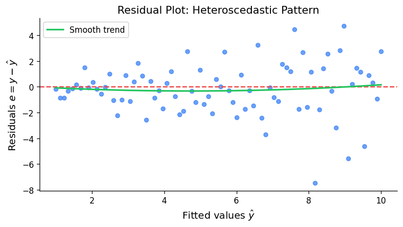
Standard diagnostic plots — residuals vs. fitted values (checking non-constant variance and non-linearity), quantile-quantile plots (checking normality), and scale-location plots — are the first line of defence against model misspecification.
Cook’s distance measures the influence of observation \(i \) by computing how much all fitted values change when it is deleted:
\[ D_i = \frac{(\hat{\boldsymbol{\beta}} - \hat{\boldsymbol{\beta}}_{(-i)})^\top \mathbf{X}^\top\mathbf{X}(\hat{\boldsymbol{\beta}} - \hat{\boldsymbol{\beta}}_{(-i)})}{(p+1)\hat\sigma^2} = \frac{e_i^2}{(p+1)\hat\sigma^2} \cdot \frac{h_{ii}}{(1-h_{ii})^2} \]Observations with \(D_i > 4/(n-p-1) \) are conventionally flagged as influential. Note that Cook’s distance couples two concerns: large residuals (poor fit) and high leverage (unusual predictor values). A high-leverage point is only influential if it also has a large residual; a perfect-fit outlier on the predictor space causes no distortion.
DFFITS and DFBETAS provide finer-grained measures of observation influence on individual fitted values and specific coefficients, respectively.
Module 3: The Bias-Variance Trade-Off
Error Decomposition
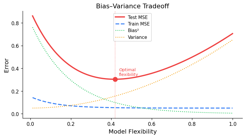
The expected prediction error at a new point \(x_0 \) can be decomposed into three irreducible components. Suppose we use a fitting procedure that produces an estimator \(\hat f(x_0) \) trained on data \(\mathcal{D} \), and the true model is \(y = f(x) + \varepsilon \) with \(\mathrm{Var}(\varepsilon) = \sigma^2 \):
\[ \mathrm{EPE}(x_0) = E\!\left[(y_0 - \hat f(x_0))^2\right] = \underbrace{\left[f(x_0) - E[\hat f(x_0)]\right]^2}_{\text{Bias}^2} + \underbrace{\mathrm{Var}(\hat f(x_0))}_{\text{Variance}} + \underbrace{\sigma^2}_{\text{Irreducible}} \]The bias measures the systematic error: how far, on average, the estimator is from the truth. The variance measures estimation instability: how much the estimator fluctuates across different training datasets. The irreducible error \(\sigma^2 \) is the noise inherent in the data-generating process and cannot be reduced by any model.
import numpy as np
import matplotlib.pyplot as plt

x = np.linspace(0, 1, 200)
complexity = np.linspace(0, 1, 200)

bias2 = np.exp(-5 * complexity)
variance = 0.05 * np.exp(4 * complexity)
irreducible = np.full_like(complexity, 0.05)
mse = bias2 + variance + irreducible

fig, ax = plt.subplots(figsize=(7, 4))
ax.plot(complexity, bias2,   label=r'Bias$^2$',          color='steelblue', lw=2)
ax.plot(complexity, variance, label='Variance',           color='tomato',    lw=2)
ax.plot(complexity, irreducible, label='Irreducible',    color='gray',      lw=1.5, ls='--')
ax.plot(complexity, mse,      label='MSE = Bias²+Var+σ²', color='black',     lw=2.5)
ax.axvline(complexity[np.argmin(mse)], color='green', ls=':', label='Optimal complexity')
ax.set_xlabel('Model Complexity')
ax.set_ylabel('Error')
ax.set_title('Bias-Variance Trade-off')
ax.legend()
plt.tight_layout()
plt.savefig('bias_variance_tradeoff.png', dpi=150)
plt.show()
Reducible vs. Irreducible Error
The key insight is that only the reducible error — the sum of bias² and variance — can be controlled through model selection. A simple model (few parameters) has high bias but low variance; a complex model (many parameters) has low bias but high variance. The optimal model minimises the total reducible error, producing a U-shaped MSE curve as a function of model complexity.
For the OLS estimator specifically, the Gauss-Markov theorem guarantees that it is the best linear unbiased estimator (BLUE): among all linear estimators with zero bias, OLS has the smallest variance. However, this optimality within the unbiased class does not mean OLS is optimal overall — biased estimators (like ridge regression) can achieve lower MSE by trading a small amount of bias for a large reduction in variance.
Module 4: Cross-Validation
The Need for Out-of-Sample Evaluation
A model’s training error (evaluated on the same data used to fit it) systematically underestimates the generalisation error (performance on new observations). Cross-validation is the standard remedy: it estimates out-of-sample performance by partitioning the available data so that evaluation never occurs on training observations.
k-Fold Cross-Validation
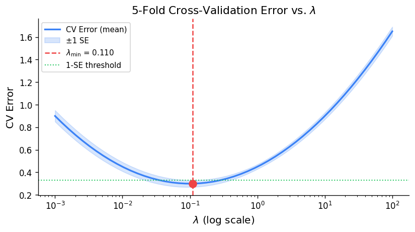
In k-fold cross-validation, the data is randomly divided into \(k \) equal-sized folds. The model is fitted on \(k-1 \) folds and evaluated on the held-out fold; this is repeated \(k \) times, and the CV error is:
\[ \text{CV}_k = \frac{1}{n}\sum_{i=1}^n \left(y_i - \hat f^{(-\kappa(i))}(x_i)\right)^2 \]where \(\hat f^{(-\kappa(i))} \) denotes the fit computed with fold \(\kappa(i) \) omitted. Common choices are \(k = 5 \) or \(k = 10 \), which balance computational cost against bias.
Leave-One-Out Cross-Validation
Leave-one-out cross-validation (LOOCV) takes \(k = n \): each observation is held out in turn. For linear smoothers (where \(\hat{\mathbf{y}} = \mathbf{S}\mathbf{y} \) for some smoother matrix \(\mathbf{S} \), there is a remarkable computational shortcut that avoids refitting the model \(n \) times. For OLS, \(\mathbf{S} = \mathbf{H} \), and the shortcut formula is:
\[ \text{CV}_{\text{LOO}} = \frac{1}{n}\sum_{i=1}^n \left(\frac{e_i}{1 - h_{ii}}\right)^2 \]where \(e_i = y_i - \hat y_i \) is the ordinary residual and \(h_{ii} \) is the \(i \)th diagonal of the hat matrix. Observations with high leverage \(h_{ii} \to 1 \) receive very large weight in LOOCV — the model fits them almost exactly, so leaving them out would dramatically change the fit.
Generalised Cross-Validation
Generalised cross-validation (GCV) replaces the individual leverages \(h_{ii} \) with their average \(\bar h = (p+1)/n \):
\[ \text{GCV} = \frac{1}{n}\sum_{i=1}^n \left(\frac{e_i}{1 - (p+1)/n}\right)^2 = \frac{\text{RSS}/n}{\left(1 - (p+1)/n\right)^2} \]GCV is computationally cheaper than LOOCV and generalises naturally beyond linear models to any smoother with a well-defined effective degrees of freedom \(\text{df} = \mathrm{tr}(\mathbf{S}) \):
\[ \text{GCV} = \frac{1}{n}\sum_{i=1}^n \left(\frac{e_i}{1 - \mathrm{tr}(\mathbf{S})/n}\right)^2 \]This formulation is particularly important for smoothing splines and kernel regression, where the smoother matrix depends on a tuning parameter.
Module 5: Variable Selection
The Challenge of Many Predictors
When \(p \) predictors are available, including all of them may overfit the data and inflate variance. The goal of variable selection is to identify a parsimonious model — using a subset of the predictors — that achieves low out-of-sample prediction error or provides interpretable inference.
Best-subset selection examines all \(2^p \) possible subsets of predictors and selects the best by some criterion. This is computationally feasible only for small \(p \) (say \(p \leq 30 \); for larger problems, greedy algorithms are the practical alternative.
Greedy Approaches
Forward stepwise selection begins with an intercept-only model and iteratively adds the predictor that most improves the fit criterion, stopping when no further improvement exceeds a threshold. It examines at most \(1 + p + (p-1) + \cdots + 1 = O(p^2) \) models, making it tractable for large \(p \).
Backward stepwise selection begins with the full model and iteratively removes the predictor whose deletion least degrades fit. It requires \(n > p \) to fit the initial model but can explore a different path through model space than forward selection.
Neither approach guarantees finding the globally best subset, but both often perform comparably to exhaustive search in practice.
Model Selection Criteria
Mallows’ Cp estimates the mean squared prediction error (scaled by \(\sigma^2 \) for a model with \(p' \) predictors:
\[ C_p = \frac{\text{RSS}_{p'}}{\hat\sigma^2} + 2p' - n \]where \(\hat\sigma^2 \) is estimated from the full model. Models with \(C_p \approx p' \) are desirable; a model with \(C_p \gg p' \) has systematic prediction bias.
Akaike’s Information Criterion (AIC) and Bayesian Information Criterion (BIC) are likelihood-based criteria applicable beyond least squares:
\[ \text{AIC} = -2\log\hat L + 2p', \qquad \text{BIC} = -2\log\hat L + p'\log n \]BIC imposes a heavier penalty on model size, favouring sparser models, especially for large \(n \). For Gaussian errors with known \(\sigma^2 \), AIC is equivalent to Cp up to a constant.
All these in-sample criteria are proxies for out-of-sample performance. They work by adjusting the training error upward to penalise complexity, approximating the expected test error without requiring a separate test set.
Module 6: Weighted Least Squares
Heteroscedastic Errors
The OLS assumption of constant error variance \(\text{Var}(\varepsilon_i) = \sigma^2 \) is frequently violated. When the variance is observation-specific, \(\text{Var}(\varepsilon_i) = \sigma^2/w_i \), with known weights \(w_i > 0 \), the weighted least squares (WLS) estimator minimises the weighted residual sum of squares:
\[ \text{WRSS}(\boldsymbol{\beta}) = \sum_{i=1}^n w_i(y_i - \mathbf{x}_i^\top\boldsymbol{\beta})^2 = (\mathbf{y} - \mathbf{X}\boldsymbol{\beta})^\top\mathbf{W}(\mathbf{y} - \mathbf{X}\boldsymbol{\beta}) \]where \(\mathbf{W} = \text{diag}(w_1, \ldots, w_n) \). The WLS estimator has the closed form:
\[ \hat{\boldsymbol{\beta}}_{\text{WLS}} = (\mathbf{X}^\top\mathbf{W}\mathbf{X})^{-1}\mathbf{X}^\top\mathbf{W}\mathbf{y} \]and satisfies \(\hat{\boldsymbol{\beta}}_{\text{WLS}} \sim \mathcal{N}(\boldsymbol{\beta}, \sigma^2(\mathbf{X}^\top\mathbf{W}\mathbf{X})^{-1}) \). Observations with larger \(w_i \) are more precise and thus receive greater influence on the fit.
Common Weighting Schemes
| Setting | Weight choice | Motivation |
|---|---|---|
| Variance proportional to a predictor | \(w_i = 1/x_i \) | Stabilise variance |
| Variance known from replication | \(w_i = n_i \) | Group means with unequal group sizes |
| Robust iterative reweighting | \(w_i = \psi(r_i/\hat\sigma)/r_i \) | Downweight outliers |
| Inverse variance known | \(w_i = 1/\sigma_i^2 \) | Meta-analysis, calibration data |
Generalised Least Squares
When errors are correlated — \(\text{Var}(\boldsymbol{\varepsilon}) = \sigma^2\boldsymbol{\Sigma} \) for a known positive-definite matrix \(\boldsymbol{\Sigma} \) — generalised least squares (GLS) achieves BLUE by transforming the problem. Since \(\boldsymbol{\Sigma} \) is positive definite, there exists a lower-triangular Cholesky factor \(\mathbf{B} \) such that \(\boldsymbol{\Sigma} = \mathbf{B}\mathbf{B}^\top \). Pre-multiplying both sides of the model by \(\mathbf{B}^{-1} \):
\[ \mathbf{B}^{-1}\mathbf{y} = \mathbf{B}^{-1}\mathbf{X}\boldsymbol{\beta} + \mathbf{B}^{-1}\boldsymbol{\varepsilon} \]yields a transformed model \(\tilde{\mathbf{y}} = \tilde{\mathbf{X}}\boldsymbol{\beta} + \tilde{\boldsymbol{\varepsilon}} \) where \(\text{Var}(\tilde{\boldsymbol{\varepsilon}}) = \sigma^2\mathbf{I} \). OLS on the transformed data gives the GLS estimator \(\hat{\boldsymbol{\beta}}_{\text{GLS}} = (\mathbf{X}^\top\boldsymbol{\Sigma}^{-1}\mathbf{X})^{-1}\mathbf{X}^\top\boldsymbol{\Sigma}^{-1}\mathbf{y} \).
Module 7: Robust Regression
The Failure of OLS under Contamination
OLS minimises the sum of squared residuals, which means even a single extreme outlier can dramatically distort the estimated regression line. The squared loss function gives unbounded influence to large residuals. Robust regression seeks estimators that are resistant to a small fraction of contaminated observations.
M-Estimators
M-estimators generalise OLS by replacing the squared loss with a more slowly growing loss function \(\rho(\cdot) \):
\[ \hat{\boldsymbol{\beta}}_M = \arg\min_{\boldsymbol{\beta}} \sum_{i=1}^n \rho\!\left(\frac{y_i - \mathbf{x}_i^\top\boldsymbol{\beta}}{\hat\sigma}\right) \]where \(\hat\sigma \) is a robust scale estimate (typically the median absolute deviation \(\hat\sigma = \mathrm{MAD}/0.6745 \). Setting the gradient to zero yields the estimating equations:
\[ \sum_{i=1}^n \psi\!\left(\frac{r_i}{\hat\sigma}\right) \mathbf{x}_i = \mathbf{0}, \quad \psi = \rho' \]Different choices of \(\psi \) define different M-estimators:
Huber’s ψ is piecewise linear, behaving like OLS for small residuals and like LAD (L1) for large ones:
\[ \psi_H(u) = \begin{cases} u & |u| \leq k \\ k\,\mathrm{sign}(u) & |u| > k \end{cases} \]with the default tuning constant \(k = 1.345 \) (giving 95% efficiency at the normal model).
Hampel’s ψ adds a descending limb for very large residuals, giving them declining weight:
\[ \psi_{\text{Hamp}}(u) = \begin{cases} u & 0 \leq |u| \leq a \\ a\,\mathrm{sign}(u) & a < |u| \leq b \\ a\,\frac{c - |u|}{c - b}\,\mathrm{sign}(u) & b < |u| \leq c \\ 0 & |u| > c \end{cases} \]Tukey’s bisquare ψ zeroes out residuals beyond a threshold, completely discarding severe outliers:
\[ \psi_T(u) = \begin{cases} u(1 - u^2/c^2)^2 & |u| \leq c \\ 0 & |u| > c \end{cases} \]with \(c = 4.685 \) for 95% efficiency. Unlike Huber, Tukey’s bisquare yields a non-convex objective and may have local minima.
import numpy as np
import matplotlib.pyplot as plt

u = np.linspace(-5, 5, 500)

# Huber psi
k = 1.345
psi_huber = np.where(np.abs(u) <= k, u, k * np.sign(u))

# Tukey bisquare psi
c_t = 4.685
psi_tukey = np.where(np.abs(u) <= c_t, u * (1 - (u/c_t)**2)**2, 0)

# OLS (for reference)
psi_ols = u

fig, ax = plt.subplots(figsize=(7, 4))
ax.plot(u, psi_ols,   label='OLS (identity)', color='gray', ls='--', lw=1.5)
ax.plot(u, psi_huber, label="Huber (k=1.345)", color='steelblue', lw=2)
ax.plot(u, psi_tukey, label="Tukey bisquare (c=4.685)", color='tomato', lw=2)
ax.axhline(0, color='black', lw=0.8)
ax.axvline(0, color='black', lw=0.8)
ax.set_xlabel('Standardised residual u')
ax.set_ylabel(r'ψ(u)')
ax.set_title('M-Estimator ψ Functions')
ax.legend()
plt.tight_layout()
plt.savefig('m_estimator_psi.png', dpi=150)
plt.show()
Iteratively Reweighted Least Squares
The M-estimating equations can be rewritten as a WLS problem by defining weights \(w_i = \psi(r_i/\hat\sigma)/r_i \):
\[ \sum_{i=1}^n w_i r_i \mathbf{x}_i = \mathbf{0} \]The Iteratively Reweighted Least Squares (IRLS) algorithm alternates between:
- Computing weights \(w_i^{(t)} = \psi(r_i^{(t)}/\hat\sigma^{(t)})/r_i^{(t)} \),
- Solving the WLS problem \(\hat{\boldsymbol{\beta}}^{(t+1)} = (\mathbf{X}^\top\mathbf{W}^{(t)}\mathbf{X})^{-1}\mathbf{X}^\top\mathbf{W}^{(t)}\mathbf{y} \),
until convergence. Each iteration is a standard WLS computation, making IRLS straightforward to implement.
The Breakdown Point and High-Breakdown Estimators
The breakdown point of an estimator is the smallest fraction of contaminated observations needed to make the estimate arbitrarily bad. OLS has a breakdown point of \(1/n \to 0 \): a single outlier can be arbitrarily influential. M-estimators improve on this but still have breakdown points tending to zero for regression.
Least Median of Squares (LMS) minimises the median of squared residuals:
\[ \hat{\boldsymbol{\beta}}_{\text{LMS}} = \arg\min_{\boldsymbol{\beta}} \;\text{median}_i\, r_i^2(\boldsymbol{\beta}) \]Least Trimmed Squares (LTS) minimises the sum of the \(\lceil n/2 \rceil \) smallest squared residuals, discarding the largest half. Both LMS and LTS achieve a breakdown point of approximately 50%: up to nearly half the data can be arbitrarily contaminated without breaking the estimator. This comes at the cost of efficiency (LTS is only 7% as efficient as OLS at the Gaussian model), so LTS is typically used as a preliminary estimator to identify outliers, followed by OLS or M-estimation on the cleaned data.
The Sensitivity Curve
The influence function (or sensitivity curve) describes how an estimator responds to a single new observation added to the data. For OLS, the influence function is unbounded — a single observation at an extreme predictor value can have arbitrarily large influence. For Tukey’s bisquare M-estimator, the influence function re-descends to zero for very large residuals, making the estimator redescending and hence robust.
Module 8: Piecewise Regression and Local Methods
Indicator Basis Functions
Piecewise regression partitions the predictor range into intervals and fits a separate polynomial on each piece, allowing the regression function to change shape abruptly. The building blocks are truncated power basis functions:
\[ (x - t)_+^q = \begin{cases} (x-t)^q & x > t \\ 0 & x \leq t \end{cases} \]A piecewise linear model with a single knot at \(t \) is:
\[ f(x) = \beta_0 + \beta_1 x + \beta_2(x-t)_+ \]This is continuous at \(t \) (no jump) but has a slope change of \(\beta_2 \). To allow a jump discontinuity (as in regression discontinuity designs), an indicator \(1(x > t) \) is added. Adding \(K \) knots \(t_1 < \cdots < t_K \) expands to:
\[ f(x) = \beta_0 + \beta_1 x + \sum_{k=1}^K \gamma_k(x - t_k)_+ \]For piecewise cubic with continuous first and second derivatives — the building blocks of splines — the basis is \(\{1, x, x^2, x^3, (x-t_1)_+^3, \ldots, (x-t_K)_+^3\} \).
K-Nearest Neighbours Regression
K-nearest neighbours (KNN) regression predicts \(f(x) \) by averaging the responses of the \(K \) training observations closest to \(x \):
\[ \hat f(x) = \frac{1}{K}\sum_{x_i \in \mathcal{N}_K(x)} y_i \]where \(\mathcal{N}_K(x) \) is the set of \(K \) nearest neighbours of \(x \). Small \(K \) gives a wiggly, low-bias fit; large \(K \) gives a smooth, low-variance fit. KNN is a special case of local constant regression (Nadaraya-Watson with a uniform kernel and bandwidth determined by the \(K \)th nearest neighbour distance).
Weighted Local Fitting
Local polynomial regression fits a polynomial of degree \(d \) at each query point \(x \) by solving a locally weighted least squares problem:
\[ \min_{a_0, \ldots, a_d} \sum_{i=1}^n K_h(x_i - x)\left(y_i - \sum_{j=0}^d a_j(x_i - x)^j\right)^2 \]where \(K_h(\cdot) = K(\cdot/h)/h \) is a kernel that downweights distant observations. The estimate at \(x \) is \(\hat f(x) = \hat a_0 \). Local linear regression (\(d=1 \) is particularly attractive because it has no boundary bias, whereas the Nadaraya-Watson estimator (\(d=0 \) suffers from boundary effects.
Module 9: Smoothing Methods
The Linear Basis Expansion Framework
Many nonparametric methods can be unified through the concept of linear basis expansion. Rather than fitting \(f \) directly, we express it as a linear combination of basis functions \(h_j(x) \):
\[ f(x) = \sum_{j=1}^M \beta_j h_j(x) \]The model is then linear in \(\boldsymbol{\beta} \), and OLS or penalised regression applies. Different choices of \(\{h_j\} \) yield different smoothers: polynomial regression, piecewise polynomials, splines, and Fourier series are all instances of this framework.
Regression Splines
Regression splines use the truncated power basis of degree \(q \) with knots \(t_1 < \cdots < t_K \):
\[ \mathcal{B} = \{1, x, x^2, \ldots, x^q,\; (x-t_1)_+^q, \ldots, (x-t_K)_+^q\} \]The resulting spline function is a piecewise polynomial of degree \(q \) that is \((q-1) \)-times continuously differentiable at each knot. Cubic splines (\(q=3 \) are the most popular: they are smooth to the eye (continuous up to the second derivative) while being computationally and analytically tractable.
Natural cubic splines add two additional boundary constraints: the function must be linear beyond the outermost knots \(t_1 \) and \(t_K \) (i.e., \(f''(x) = 0 \) for \(x < t_1 \) and \(x > t_K \). These constraints reduce the effective degrees of freedom from \(K + q + 1 \) to \(K \) and improve behaviour at the boundaries where data is sparse. Natural cubic splines are asymptotically optimal among all smoothers in MISE.
B-splines (basis splines) provide a numerically superior representation of the same spline space. Each B-spline basis function is locally supported (non-zero only on a few consecutive knot intervals), making the resulting design matrix banded and linear system computationally efficient. The B-spline basis is preferable to the truncated power basis for numerical implementation, though both span the same function space.
Smoothing Splines
Rather than fixing the knot locations in advance, smoothing splines place a knot at every observed data point and regularise the fit through a roughness penalty. The estimator is the minimiser of:
\[ \text{PRSS}(f, \lambda) = \sum_{i=1}^n (y_i - f(x_i))^2 + \lambda \int_a^b [f''(t)]^2\, dt \]The tuning parameter \(\lambda \geq 0 \) controls the bias-variance trade-off: \(\lambda = 0 \) interpolates the data, and \(\lambda \to \infty \) forces \(f \) to be linear. The remarkable fact is that the exact minimiser of this infinite-dimensional problem is a natural cubic spline with knots at the observed data points. This means the solution is computable in finite dimensions.
The smoothing spline estimator is a linear smoother: \(\hat{\mathbf{y}} = \mathbf{S}_\lambda \mathbf{y} \), where the smoother matrix is:
\[ \mathbf{S}_\lambda = \mathbf{N}(\mathbf{N}^\top\mathbf{N} + \lambda\boldsymbol{\Omega}_N)^{-1}\mathbf{N}^\top \]Here \(\mathbf{N} \) is the matrix of natural spline basis functions evaluated at the data points, and \(\boldsymbol{\Omega}_N \) is the penalty matrix with entries \(\{\boldsymbol{\Omega}_N\}_{jk} = \int N_j''(t)N_k''(t)\,dt \).
Eigendecomposition of the Smoother Matrix
Since \(\mathbf{S}_\lambda \) is symmetric and positive semi-definite, it has a real eigendecomposition \(\mathbf{S}_\lambda = \mathbf{U}\mathbf{D}_\lambda\mathbf{U}^\top \) with eigenvalues:
\[ d_k(\lambda) = \frac{1}{1 + \lambda \rho_k} \]where \(\rho_k \geq 0 \) are the eigenvalues of the penalty matrix. The eigenvectors \(\mathbf{u}_k \) (Demmler-Reinsch basis) are ordered from smoothest to roughest. Smooth components (small \(\rho_k \) are nearly unshrunken (\(d_k \approx 1 \); rough components (large \(\rho_k \) are heavily shrunk toward zero. The first two eigenvectors always correspond to the intercept and linear trend, which have zero roughness penalty (\(\rho_1 = \rho_2 = 0 \), \(d_1 = d_2 = 1 \).
The effective degrees of freedom of the smoothing spline is:
\[ \text{df}_\lambda = \mathrm{tr}(\mathbf{S}_\lambda) = \sum_{k=1}^n d_k(\lambda) = \sum_{k=1}^n \frac{1}{1+\lambda\rho_k} \]As \(\lambda \) increases from 0 to \(\infty \), \(\text{df}_\lambda \) decreases from \(n \) to 2. Users can equivalently specify a target degrees of freedom and solve for the corresponding \(\lambda \).
Bandwidth Selection for Smoothing Splines
The LOOCV criterion for the smoothing spline has the same shortcut form as for OLS:
\[ \text{CV}_\text{LOO}(\lambda) = \frac{1}{n}\sum_{i=1}^n \left(\frac{y_i - \hat f_\lambda(x_i)}{1 - \{S_\lambda\}_{ii}}\right)^2 \]and GCV replaces individual diagonal entries with their mean:
\[ \text{GCV}(\lambda) = \frac{\text{RSS}(\lambda)/n}{\left(1 - \text{df}_\lambda/n\right)^2} \]In practice, GCV is the standard default in R’s smooth.spline() function.
import numpy as np
import matplotlib.pyplot as plt

np.random.seed(42)
x = np.linspace(0, 1, 100)
f_true = np.sin(2 * np.pi * x)
y = f_true + 0.3 * np.random.randn(100)

# Simulate smoothing spline effect at different lambda
from scipy.interpolate import UnivariateSpline
lambdas = [1e-5, 1e-3, 0.1]
labels  = ['λ small (overfit)', 'λ optimal', 'λ large (underfit)']
colors  = ['tomato', 'steelblue', 'green']

fig, axes = plt.subplots(1, 3, figsize=(12, 4), sharey=True)
for ax, lam, lab, col in zip(axes, lambdas, labels, colors):
    spl = UnivariateSpline(x, y, s=lam*len(x))
    ax.scatter(x, y, s=10, color='gray', alpha=0.5)
    ax.plot(x, f_true, 'k--', lw=1.5, label='True f')
    ax.plot(x, spl(x), color=col, lw=2, label=lab)
    ax.set_title(lab)
    ax.legend(fontsize=8)
    ax.set_xlabel('x')
axes[0].set_ylabel('y')
plt.suptitle('Smoothing Spline at Different λ')
plt.tight_layout()
plt.savefig('smoothing_splines.png', dpi=150)
plt.show()
Multidimensional Smoothing
When the predictors are multivariate \(\mathbf{x} = (x_1, \ldots, x_d) \), several extensions are available.
Tensor product splines construct a basis by taking all products of univariate spline bases in each dimension: \(\{h_{j_1}(x_1) \cdot h_{j_2}(x_2) : j_1 = 1,\ldots,M_1,\; j_2 = 1,\ldots,M_2\} \). The number of basis functions grows exponentially with dimension — the curse of dimensionality.
Thin-plate splines generalise smoothing splines to multiple dimensions by penalising all mixed partial derivatives of order \(m \). For \(d=2 \) with \(m=2 \), the penalty is:
\[ J_2(f) = \iint \left[\left(\frac{\partial^2 f}{\partial x_1^2}\right)^2 + 2\left(\frac{\partial^2 f}{\partial x_1 \partial x_2}\right)^2 + \left(\frac{\partial^2 f}{\partial x_2^2}\right)^2\right] dx_1\, dx_2 \]Thin-plate splines are radially symmetric (rotation-invariant) and do not require the user to specify a product structure, but they are computationally intensive for large \(n \).
Additive Models and GAMs
Additive models sidestep the curse of dimensionality by assuming the regression function decomposes as a sum of univariate terms:
\[ y = \alpha + \sum_{j=1}^p f_j(x_j) + \varepsilon \]where each \(f_j \) is an arbitrary smooth function. Generalised Additive Models (GAMs) extend this to non-Gaussian responses through a link function \(g(\mu) = \alpha + \sum_j f_j(x_j) \). The component functions are estimated by the backfitting algorithm: repeatedly cycle through predictors, fitting each \(f_j \) by applying a univariate smoother to the partial residuals \(y_i - \hat\alpha - \sum_{k \neq j} \hat f_k(x_{ik}) \), until convergence.
The additive assumption sacrifices interaction terms but allows the model to handle moderate-dimensional problems without parametric constraints. In R, GAMs are implemented via the gam package (Hastie and Tibshirani) or mgcv (Wood), using penalised regression splines.
Kernel Smoothing and the Nadaraya-Watson Estimator
Kernel regression estimates \(f(x) = E[y|X=x] \) directly as a locally weighted average. The Nadaraya-Watson estimator is:
\[ \hat f(x) = \frac{\sum_{i=1}^n K_h(x_i - x)\, y_i}{\sum_{i=1}^n K_h(x_i - x)} \]where \(K_h(u) = K(u/h)/h \) is a kernel function scaled by bandwidth \(h \). Common kernels include the Gaussian \(K(u) = \phi(u) \), Epanechnikov \(K(u) = \frac{3}{4}(1-u^2)_+ \) (MSE-optimal), and tricube \(K(u) = \frac{70}{81}(1-|u|^3)_+^3 \) (used in LOESS). The bias of the Nadaraya-Watson estimator at the boundary is of order \(O(h) \), larger than in the interior, motivating local linear regression.
LOESS (Locally Weighted Scatter Plot Smoother)
LOESS (or LOWESS, Cleveland 1979) fits a local polynomial of degree \(d \) at each \(x \), using the tricube kernel with the bandwidth determined by the nearest-neighbour fraction \(\alpha \):
\[ h_i(x) = \text{(distance to the }\lfloor \alpha n \rfloor\text{-th nearest neighbour of } x) \]The span \(\alpha \in (0,1] \) controls smoothness: large \(\alpha \) uses more neighbours and produces smoother fits. LOESS is the default smoother in R’s geom_smooth() with method="loess".
Comparing LOESS and Smoothing Splines via SVD
Both LOESS and smoothing splines are linear smoothers: \(\hat{\mathbf{y}} = \mathbf{S}\mathbf{y} \). The SVD of \(\mathbf{S} \) reveals their structure:
\[ \mathbf{S} = \mathbf{U}\mathbf{D}\mathbf{V}^\top \]For a symmetric smoother matrix (smoothing splines), \(\mathbf{U} = \mathbf{V} \) and this is an eigendecomposition. LOESS has an asymmetric smoother matrix; its SVD reveals which linear combinations of responses it preferentially amplifies. In practice, the effective degrees of freedom for both smoothers is approximately \(\mathrm{tr}(\mathbf{S}) \), providing a unified scale for comparison.
Module 10: Shrinkage Estimators
Ridge Regression
When predictors are correlated (multicollinearity), \(\mathbf{X}^\top\mathbf{X} \) becomes nearly singular, and OLS estimates have inflated variance. Ridge regression adds a ridge penalty to the objective:
\[ \hat{\boldsymbol{\beta}}_R(\lambda) = \arg\min_{\boldsymbol{\beta}} \left\{\|\mathbf{y} - \mathbf{X}\boldsymbol{\beta}\|^2 + \lambda\|\boldsymbol{\beta}\|^2\right\} \]The closed-form solution is:
\[ \hat{\boldsymbol{\beta}}_R(\lambda) = (\mathbf{X}^\top\mathbf{X} + \lambda\mathbf{I})^{-1}\mathbf{X}^\top\mathbf{y} \]Adding \(\lambda\mathbf{I} \) to \(\mathbf{X}^\top\mathbf{X} \) ensures the matrix is invertible for all \(\lambda > 0 \), regardless of multicollinearity. Ridge regression shrinks all coefficients toward zero simultaneously, with more shrinkage for coefficients corresponding to directions of small variation in the predictors.
The SVD representation illuminates ridge’s mechanism. With \(\mathbf{X} = \mathbf{U}\mathbf{D}\mathbf{V}^\top \):
\[ \hat{\boldsymbol{\beta}}_R = \mathbf{V}\mathrm{diag}\!\left(\frac{d_j}{d_j^2 + \lambda}\right)\mathbf{U}^\top\mathbf{y} \]Each singular value component is shrunk by the factor \(d_j^2/(d_j^2 + \lambda) \). Small singular values (directions of near-collinearity) are shrunk most. The effective degrees of freedom is:
\[ \text{df}(\lambda) = \mathrm{tr}\!\left[\mathbf{X}(\mathbf{X}^\top\mathbf{X} + \lambda\mathbf{I})^{-1}\mathbf{X}^\top\right] = \sum_{j=1}^p \frac{d_j^2}{d_j^2 + \lambda} \]At \(\lambda=0 \), \(\text{df} = p \) (OLS); as \(\lambda \to \infty \), \(\text{df} \to 0 \).
It is critical to standardise predictors before applying ridge (and LASSO): otherwise the penalty treats predictors on different scales unequally.
The LASSO
The LASSO (Least Absolute Shrinkage and Selection Operator, Tibshirani 1996) replaces the L2 penalty with an L1 penalty:
\[ \hat{\boldsymbol{\beta}}_L(\lambda) = \arg\min_{\boldsymbol{\beta}} \left\{\|\mathbf{y} - \mathbf{X}\boldsymbol{\beta}\|^2 + \lambda\|\boldsymbol{\beta}\|_1\right\} \]Unlike ridge, the LASSO has no closed-form solution for \(p > 1 \). For the orthonormal design case, the LASSO solution is soft thresholding: \(\hat\beta_j = \text{sign}(\hat\beta_j^\text{OLS})(|\hat\beta_j^\text{OLS}| - \lambda)_+ \). In general, LASSO solutions must be obtained by convex optimisation.
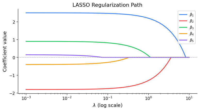
The crucial difference from ridge is sparsity: the L1 penalty has a corner at zero, so the optimal solution sets some coefficients exactly to zero — the LASSO performs automatic variable selection. As \(\lambda \) increases from 0, predictors enter (or leave) the model at discrete thresholds, tracing a regularisation path.
import numpy as np
import matplotlib.pyplot as plt

# Conceptual ridge vs LASSO coefficient paths
lambdas = np.logspace(-2, 2, 200)

# Simulate: suppose beta_OLS = [2, -1, 0.5, -0.1, 0.05]
beta_ols = np.array([2.0, -1.0, 0.5, -0.1, 0.05])
colors_coef = ['steelblue', 'tomato', 'green', 'orange', 'purple']
labels_coef = [f'β{j+1} (OLS={b:.2f})' for j, b in enumerate(beta_ols)]

fig, axes = plt.subplots(1, 2, figsize=(12, 5))

# Ridge: continuous shrinkage
for j, (b, c, lab) in enumerate(zip(beta_ols, colors_coef, labels_coef)):
    # X'X ~ I approximation for illustration
    ridge_path = b / (1 + lambdas)
    axes[0].plot(lambdas, ridge_path, color=c, label=lab, lw=2)
axes[0].axhline(0, color='gray', lw=0.8)
axes[0].set_xscale('log')
axes[0].set_xlabel('λ')
axes[0].set_ylabel('Coefficient value')
axes[0].set_title('Ridge Regularisation Path')
axes[0].legend(fontsize=7)

# LASSO: soft thresholding (orthonormal X approximation)
for j, (b, c, lab) in enumerate(zip(beta_ols, colors_coef, labels_coef)):
    lasso_path = np.sign(b) * np.maximum(np.abs(b) - lambdas * 0.1, 0)
    axes[1].plot(lambdas * 0.1, lasso_path, color=c, label=lab, lw=2)
axes[1].axhline(0, color='gray', lw=0.8)
axes[1].set_xlabel('λ')
axes[1].set_ylabel('Coefficient value')
axes[1].set_title('LASSO Regularisation Path (sparse solutions)')
axes[1].legend(fontsize=7)

plt.tight_layout()
plt.savefig('ridge_lasso_paths.png', dpi=150)
plt.show()
The Elastic Net
The elastic net (Zou and Hastie 2005) combines ridge and LASSO penalties:
\[ \hat{\boldsymbol{\beta}}_{\text{EN}} = \arg\min_{\boldsymbol{\beta}} \left\{\|\mathbf{y} - \mathbf{X}\boldsymbol{\beta}\|^2 + \lambda_1\|\boldsymbol{\beta}\|_1 + \lambda_2\|\boldsymbol{\beta}\|^2\right\} \]The L1 component induces sparsity (variable selection) while the L2 component handles correlated predictors by encouraging grouped selection: correlated predictors tend to enter or leave the model together, rather than one arbitrarily dominating. The elastic net strictly contains both ridge (\(\lambda_1 = 0 \) and LASSO (\(\lambda_2 = 0 \) as special cases.
In R, all three methods are efficiently implemented via the glmnet package (Friedman, Hastie, and Tibshirani 2010), which computes the full regularisation path using coordinate descent. The mixing parameter \(\alpha \in [0,1] \) in glmnet controls the ridge-LASSO mix: \(\alpha=0 \) is pure ridge, \(\alpha=1 \) is pure LASSO.
library(glmnet)
# fit LASSO path
fit <- glmnet(X, y, alpha = 1)  # LASSO
plot(fit, xvar = "lambda", label = TRUE)
# cross-validated lambda
cv_fit <- cv.glmnet(X, y, alpha = 1)
best_lambda <- cv_fit$lambda.1se
coef(cv_fit, s = "lambda.1se")
Module 11: Kernel Density Estimation
The Kernel Density Estimator
Given an i.i.d. sample \(u_1, \ldots, u_n \sim f \), the kernel density estimator (KDE) is:
\[ \hat f_h(u) = \frac{1}{nh}\sum_{i=1}^n K\!\left(\frac{u - u_i}{h}\right) \]where \(K \) is a symmetric kernel (typically \(\int K = 1 \), \(K \geq 0 \) and \(h > 0 \) is the bandwidth. The estimator places a scaled kernel centred at each data point and sums them up, yielding a smooth estimate of the density.
Bias-Variance Analysis
For a fixed point \(u \), the pointwise MSE of the KDE is:
\[ \mathrm{MSE}[\hat f_h(u)] = \left(\mathrm{Bias}[\hat f_h(u)]\right)^2 + \mathrm{Var}[\hat f_h(u)] \]Under standard smoothness conditions on \(f \), as \(h \to 0 \) and \(nh \to \infty \):
\[ \mathrm{Bias}[\hat f_h(u)] \approx \frac{h^2}{2} f''(u) \int u^2 K(u)\,du = \frac{h^2 \kappa_2(K)}{2} f''(u) \]\[ \mathrm{Var}[\hat f_h(u)] \approx \frac{f(u)}{nh} R(K), \quad R(K) = \int K^2(u)\,du \]The bias grows with \(h^2 \) (oversmoothing), and the variance decays as \(1/(nh) \) (more data → less variance). The asymptotic mean integrated squared error (AMISE) integrates over all \(u \):
\[ \mathrm{AMISE}(h) = \frac{h^4 \kappa_2(K)^2}{4}\int [f''(u)]^2\,du + \frac{R(K)}{nh} \]Minimising over \(h \) gives the optimal bandwidth:
\[ h_\text{AMISE} = \left(\frac{R(K)}{\kappa_2(K)^2 \int [f''(u)]^2\,du}\right)^{1/5} n^{-1/5} \]The rate \(n^{-1/5} \) is characteristic of one-dimensional density estimation: slower than the parametric \(n^{-1/2} \) rate, reflecting the difficulty of nonparametric estimation.
The Epanechnikov kernel \(K_E(u) = \frac{3}{4}(1-u^2)\mathbf{1}_{|u|\leq 1} \) minimises AMISE among all kernel functions, providing a theoretical benchmark. In practice, the choice of kernel matters little compared to the choice of bandwidth.
import numpy as np
import matplotlib.pyplot as plt
from scipy.stats import gaussian_kde

np.random.seed(42)
# Bimodal sample
n = 300
sample = np.concatenate([np.random.normal(-2, 0.8, n//2),
                          np.random.normal(2, 0.8, n//2)])

u_grid = np.linspace(-6, 6, 400)
# True density
from scipy.stats import norm
f_true = 0.5 * norm.pdf(u_grid, -2, 0.8) + 0.5 * norm.pdf(u_grid, 2, 0.8)

fig, axes = plt.subplots(1, 3, figsize=(13, 4), sharey=True)
for ax, bw, title in zip(axes,
                         [0.2, 0.7, 2.0],
                         ['h small (undersmooth)', 'h optimal', 'h large (oversmooth)']):
    kde = gaussian_kde(sample, bw_method=bw)
    ax.hist(sample, bins=30, density=True, color='lightgray', alpha=0.6, label='Data')
    ax.plot(u_grid, f_true, 'k--', lw=1.5, label='True f')
    ax.plot(u_grid, kde(u_grid), 'steelblue', lw=2, label=f'KDE h={bw}')
    ax.set_title(title)
    ax.legend(fontsize=7)
    ax.set_xlabel('u')
axes[0].set_ylabel('Density')
plt.suptitle('Kernel Density Estimation at Different Bandwidths')
plt.tight_layout()
plt.savefig('kde_bandwidths.png', dpi=150)
plt.show()
The Nadaraya-Watson Regression Estimator
Kernel ideas extend directly to regression. The Nadaraya-Watson estimator can be derived as follows: assume \((X, Y) \) have a joint density, and estimate both the joint and marginal densities with the same kernel:
\[ \hat f(x) = \frac{\hat f_{X,Y}(x, y) \text{ integrated over }y}{\hat f_X(x)} = \frac{\sum_i K_h(x_i - x) y_i}{\sum_i K_h(x_i - x)} \]This directly motivates the estimator as the kernel-weighted average of responses near \(x \). The bandwidth for regression is selected by cross-validation using the ISE or equivalently the pseudo-likelihood criterion:
\[ h^* = \arg\min_h \text{CV}(h) = \arg\min_h \int [\hat f_h(u)]^2\,du - \frac{2}{n}\sum_{i=1}^n \hat f_{h,-i}(u_i) \]where \(\hat f_{h,-i} \) is the leave-one-out density estimate. The first term (squared integral of the estimate) penalises rough estimates, while the second term rewards fit to the data.
Module 12: Estimating an Intensity Function
Neural Spike Trains
This module applies the smoothing methods developed throughout the course to a specific problem in computational neuroscience: estimating the firing rate of a neuron from repeated experimental trials.
In a typical electrophysiology experiment, a stimulus is applied to a subject repeatedly across \(m \) trials over an observation window \([0, T] \). In each trial \(i \), the neuron generates \(n_i \) action potentials (spikes) at times \(t_{i,1}, \ldots, t_{i,n_i} \). The spike train is a random point process, and the goal is to estimate its underlying intensity function \(\lambda(t) \) — the instantaneous probability of firing per unit time.
The Peri-Stimulus Time Histogram
The Peri-Stimulus Time Histogram (PSTH) is the classical estimator: the observation window is divided into equal bins of width \(\Delta \), and the count of spikes across all trials in bin \(k \) is divided by \(m \cdot \Delta \) to estimate the average firing rate:
\[ \hat\lambda_k = \frac{\text{(total spikes in bin }k\text{)}}{m \cdot \Delta} \]The PSTH is simply a histogram estimator applied to the pooled spike times. Its limitation is the familiar bias-variance trade-off: small bins (narrow \(\Delta \) give noisy estimates; large bins smooth away temporal structure. Additionally, the PSTH must be followed by a separate smoothing step, introducing two bandwidth choices.
Poisson Process Models
The standard model for spike generation is the Poisson process. A homogeneous Poisson process on \([0,T] \) with constant rate \(\lambda \) satisfies:
- Spike counts in disjoint intervals are independent,
- The number of spikes in any interval of length \(s \) follows a Poisson distribution with mean \(\lambda s \).
The inhomogeneous (non-homogeneous) Poisson process allows the rate to vary: the expected number of spikes in \([a,b] \) is \(\int_a^b \lambda(t)\,dt \). The conditional intensity function (CIF) \(\lambda(t|\mathcal{H}_t) \) generalises this further to allow spike history \(\mathcal{H}_t \) to influence future rates, capturing refractoriness (the neuron cannot fire immediately after a spike) and bursting patterns.
Multiscale Penalized Likelihood (Recursive Dyadic Partitioning)
The multiscale approach of Kolaczyk and Nowak (2004, 2005), with neuroscience applications by Ramezan et al. (2014), avoids the two-step histogram-then-smooth procedure by directly estimating a piecewise-constant intensity function of varying resolution.
The observation window \([0,T] \) is recursively bisected into a binary tree of sub-intervals. Setting \(N = 2^J \) leaves at the bottom of the tree, the splitting proceeds as follows: at each node, the interval is split at its midpoint, producing two child intervals. Let \(X_{jk} \) denote the spike count in the sub-interval at depth \(j \) and position \(k \). By the Thinning Property of Poisson processes:
\[ X_{jk} \mid X_{j-1,\lfloor k/2\rfloor} \sim \text{Binomial}\!\left(X_{j-1,\lfloor k/2\rfloor},\; p_{jk}\right) \]where \(p_{jk} \) is the proportion of the parent interval’s expected count in the left child. Under the piecewise-constant assumption, \(p_{jk} = 1/2 \), but the model learns adaptive proportions from the data.
The tree is built top-down (recursive splitting) and pruned bottom-up using a penalised likelihood criterion that tests, at each internal node, whether to merge two children back into a constant block:
\[ \text{decision: merge or not? compare } \log L(\text{merged}) + \lambda \text{ vs } \log L(\text{split}) \]A small penalty \(\lambda \) allows many splits (detailed histogram); a large \(\lambda \) forces aggressive merging (smooth estimate). The tuning parameters \(N = 2^J \) (maximum resolution) and \(\lambda \) (penalty) are selected by leave-one-trial-out cross-validation:
\[ (N^*, \lambda^*)_{\text{ISE}} = \arg\min_{N,\lambda} \left\{\int_0^T \left[\frac{1}{m}\sum_{i=1}^m \hat c_i(t)\right]^2 dt - \frac{2}{m}\sum_{i=1}^m \frac{1}{n_i(m-1)}\sum_{\ell=1}^{n_i}\sum_{j\neq i}\hat c_j(t_{i\ell})\right\} \]where \(\hat c_i(t) \) is the estimate of \(c(t) = m\lambda(t) \) based on trial \(i \) alone. The RDP estimator is implemented in the mmnst R package as PoissonRDP.
Alternative cross-validation approaches include: leave-one-spike-out on pooled data, per-trial cross-validation with the mode of \(N_i \), or replacing ISE with Kullback-Leibler divergence as the discrepancy measure.
Goodness of Fit: The Time Rescaling Theorem
A discretised version of the Time Rescaling Theorem (Brown, Barbieri, et al.) converts the fitted intensity function into a test of model adequacy. If \(\hat\lambda(t) \) is the true intensity, then the rescaled inter-spike intervals:
\[ z_k = 1 - \exp\!\left(-\int_{t_{k-1}}^{t_k} \hat\lambda(s)\,ds\right) \]should be i.i.d. Uniform(0,1) if the model is correct. A probability-probability (pp) plot of the empirical CDF of \(\{z_k\} \) against the uniform CDF provides a visual goodness-of-fit test; departure from the diagonal, especially outside Kolmogorov-Smirnov confidence bands, indicates misfit.
Bayesian Adaptive Regression Splines (BARS)
An alternative to the multiscale approach is the BARS model of DiMatteo, Genovese, and Kass (2001), which uses free-knot regression splines in a Bayesian framework.
The key challenge in regression spline fitting is that the number and location of knots are unknown. Rather than fixing knots in advance or placing them densely (as smoothing splines do), BARS treats the knots as random variables and estimates their distribution from the data.
In the Bayesian framework, all parameters are random variables with prior distributions. The posterior distribution \(g(\theta|\mathbf{x}) \) combines prior knowledge \(p(\theta) \) with the likelihood of the observed data:
\[ g(\theta|\mathbf{x}) = \frac{f(\mathbf{x}|\theta)\, p(\theta)}{m(\mathbf{x})} \propto f(\mathbf{x}|\theta)\, p(\theta) \]In short: posterior \(\propto \) likelihood \(\times \) prior. Since the normalising constant \(m(\mathbf{x}) = \int f(\mathbf{x}|\theta)p(\theta)\,d\theta \) is often intractable, Markov Chain Monte Carlo (MCMC) methods generate samples from the posterior without requiring \(m(\mathbf{x}) \). From a large MCMC sample, the posterior mean or mode gives a point estimate of \(\theta \).
In BARS, the model is:
\[ \mu(x) = \sum_{j=1}^{k+2} \beta_j b_j(x) \]where \(b_j \) are cubic B-spline basis functions, \(k \) is the (random) number of inner knots, and \(\boldsymbol{\xi} = (\xi_1, \ldots, \xi_k) \) are the (random) knot locations. The joint prior factorises as:
\[ p(\boldsymbol{\beta}, k, \boldsymbol{\xi}, \sigma) = p_\beta(\boldsymbol{\beta}|\boldsymbol{\xi}, k, \sigma)\, p_\xi(\boldsymbol{\xi}|k)\, p_k(k)\, p_\sigma(\sigma) \]Conditionally on \((k, \boldsymbol{\xi}) \), the model is a standard linear regression. The hard part is the joint inference on \((k, \boldsymbol{\xi}) \), which lives in a variable-dimension space — ordinary MCMC cannot move between models of different dimension.
Reversible-jump MCMC (RJMCMC), introduced by Green (1995), handles variable-dimension posteriors by proposing three types of moves at each iteration:
- Birth: add a new knot at a proposed location,
- Death: remove an existing knot,
- Relocation: move an existing knot to a new position.
Each move is accepted with a Metropolis-Hastings probability that accounts for the change in dimensionality. The chain produces a sequence of spline fits of varying complexity; the posterior mean over this sequence provides the final estimate, naturally averaging over the uncertainty in knot number and location.
BARS correctly identifies the number and location of knots even at moderate signal-to-noise ratios. Its main drawback is computational cost: RJMCMC requires many iterations to explore the knot space, making BARS impractical for large datasets. The multiscale RDP approach is computationally faster and can handle data with structural zeros (bins with no spikes due to biological refractoriness).
