Chapter 1: Review of Elementary Probability

1.1 Probability Functions and Axioms

A probability function (or probability measure) \(P\) assigns a number to each event in a sample space \(\Omega\) and must satisfy three defining conditions:

1. \(P(A) \geq 0\) for every event \(A\).
2. \(P(\Omega) = 1\).
3. For mutually exclusive events \(A_1, A_2, \ldots\), \(P\!\left(\bigcup_{i} A_i\right) = \sum_i P(A_i)\).

From these axioms, the complement rule follows immediately:

\[ P(A^c) = 1 - P(A). \]

Conditional probability is defined for events \(A\) and \(B\) with \(P(B) > 0\) as

\[ P(A \mid B) = \frac{P(A \cap B)}{P(B)}. \]

Rearranging gives the multiplication rule:

\[ P(A \cap B) = P(A \mid B)\, P(B). \]

More generally, for \(n\) events \(A_1, A_2, \ldots, A_n\), the generalized multiplication rule is

\[ P(A_1 \cap A_2 \cap \cdots \cap A_n) = P(A_1)\, P(A_2 \mid A_1)\, P(A_3 \mid A_1 \cap A_2) \cdots \]

Law of Total Probability

If the sample space \(\Omega\) can be partitioned into mutually exclusive events \(B_1, B_2, \ldots, B_n\) (so \(\Omega = B_1 \cup \cdots \cup B_n\), \(B_i \cap B_j = \varnothing\) for \(i \neq j\)), then for any event \(A\):

\[ P(A) = \sum_{i=1}^{n} P(A \mid B_i)\, P(B_i). \]

This expresses \(P(A)\) as a weighted average of conditional probabilities.

Bayes’ Theorem

Combining conditional probability with the law of total probability yields Bayes’ theorem:

\[ P(B_k \mid A) = \frac{P(A \mid B_k)\, P(B_k)}{\sum_{i=1}^{n} P(A \mid B_i)\, P(B_i)}. \]

1.2 Random Variables and Their Distributions

A random variable (RV) \(X\) is a function from the sample space to the real numbers. The two main types are:

• Discrete — \(X\) takes on a finite or countably infinite set of values.
• Continuous — \(X\) takes on values in a continuum.

Discrete Random Variables

The probability mass function (PMF) of a discrete RV \(X\) is

\[ p(x) = P(X = x). \]

The cumulative distribution function (CDF) is

\[ F(a) = P(X \leq a) = \sum_{x \leq a} p(x), \]

and the complementary CDF (tail probability) is

\[ \bar{F}(a) = P(X > a) = 1 - F(a). \]

Special Discrete Distributions

The course reviews the following standard discrete distributions:

Distribution	PMF \(p(x)\)	Mean	Variance
Bernoulli\((p)\)	\(p^x(1-p)^{1-x}\), \(x\in\{0,1\}\)	\(p\)	\(p(1-p)\)
Binomial\((n,p)\)	\(\binom{n}{x}p^x(1-p)^{n-x}\), \(x=0,\ldots,n\)	\(np\)	\(np(1-p)\)
Negative Binomial\((k,p)\)	\(\binom{x-1}{k-1}p^k(1-p)^{x-k}\), \(x=k,k+1,\ldots\)	\(k/p\)	\(k(1-p)/p^2\)
Geometric\((p)\)	\((1-p)^{x-1}p\), \(x=1,2,\ldots\)	\(1/p\)	\((1-p)/p^2\)
Poisson\((\lambda)\)	\(e^{-\lambda}\lambda^x/x!\), \(x=0,1,2,\ldots\)	\(\lambda\)	\(\lambda\)
Hypergeometric\((N,r,n)\)	\(\binom{r}{x}\binom{N-r}{n-x}/\binom{N}{n}\)	\(nr/N\)	—

The table above shows the PMF, mean, and variance for each distribution. Two additional notes from the slides:

• Discrete Uniform \(\text{DU}(a, b)\): \(p(x) = \frac{1}{b-a+1}\) for \(x = a, a+1, \ldots, b\), where \(a \leq b\) are integers.
• Recovering the PMF from the CDF: If \(X\) takes values \(a_1 < a_2 < a_3 < \cdots\) with \(p(a_i) > 0\), then \(p(a_1) = F(a_1)\) and \(p(a_i) = F(a_i) - F(a_{i-1})\) for \(i \geq 2\).

The Poisson as a Limiting Binomial

One of the important results in the review is that the Poisson distribution is the limiting form of the binomial. If \(X \sim \text{Binomial}(n, p)\) and we let \(n \to \infty\) with \(np = \lambda\) held fixed (so \(p = \lambda/n \to 0\)), then

\[ P(X = x) = \binom{n}{x}\left(\frac{\lambda}{n}\right)^x\!\left(1 - \frac{\lambda}{n}\right)^{n-x} \;\xrightarrow{n\to\infty}\; \frac{e^{-\lambda}\lambda^x}{x!}, \]

which is the Poisson PMF. The key step uses the limit definition of the exponential function, \(e^z = \lim_{n\to\infty}(1 + z/n)^n\).

Continuous Random Variables

A continuous RV has a probability density function (PDF) \(f(x)\) satisfying \(f(x) \geq 0\) and \(\int_{-\infty}^{\infty} f(x)\,dx = 1\). The CDF is

\[ F(a) = \int_{-\infty}^{a} f(x)\,dx, \]

and the PDF is recovered by differentiation: \(f(x) = F'(x)\).

Common continuous distributions include the Uniform\((a,b)\), Beta\((m,n)\), Gamma (Erlang), Exponential, and Normal distributions. The Exponential\((\lambda)\) is obtained from the Erlang by taking \(n=1\), giving PDF \(f(x) = \lambda e^{-\lambda x}\) for \(x > 0\).

1.3 Expectation and Moments

For a function \(g\), the expected value of \(g(X)\) is

\[ E[g(X)] = \begin{cases} \sum_x g(x)\,p(x) & \text{discrete},\\[4pt] \int_{-\infty}^{\infty} g(x)\,f(x)\,dx & \text{continuous}. \end{cases} \]

Special cases:

• Setting \(g(x) = x^n\) gives the \(n\)-th moment \(E[X^n]\). When \(n=1\), this is the mean \(\mu = E[X]\).
• Setting \(g(x) = (x - \mu)^2\) gives the variance: \(\text{Var}(X) = E[X^2] - (E[X])^2\).
• For a linear function \(aX + b\): \(E[aX+b] = aE[X]+b\) and \(\text{Var}(aX+b) = a^2\text{Var}(X)\).
• For a linear combination \(aX + bY\): \(E[aX+bY] = aE[X] + bE[Y]\) and

\[ \text{Var}(aX + bY) = a^2\text{Var}(X) + b^2\text{Var}(Y) + 2ab\,\text{Cov}(X,Y). \]

The covariance satisfies \(\text{Cov}(X,Y) = E[XY] - E[X]E[Y]\) and \(\text{Cov}(X,X) = \text{Var}(X)\).

Moment-Generating Functions

Key properties of the MGF:

1. Moment extraction: \(E[X^n] = \phi_X^{(n)}(0)\), the \(n\)-th derivative of \(\phi_X\) evaluated at \(t=0\).
2. Uniqueness: If two RVs have the same MGF, they have the same distribution.
3. Taylor series representation: Expanding \(e^{tX}\) in a Taylor series and taking expectations gives

\[ \phi_X(t) = \sum_{n=0}^{\infty} \frac{E[X^n]}{n!}\, t^n. \]

Example — Binomial MGF. If \(X \sim \text{Binomial}(n,p)\), then

\[ \phi_X(t) = (pe^t + 1 - p)^n. \]

Differentiating and evaluating at \(t=0\) yields \(E[X] = np\) and \(\text{Var}(X) = np(1-p)\), confirming the known formulas.

1.4 Joint Distributions

For two RVs \(X\) and \(Y\), the joint CDF is \(F(a,b) = P(X \leq a, Y \leq b)\). In the discrete case, the joint PMF is \(p(x,y) = P(X=x, Y=y)\), and marginal PMFs are obtained by summing:

\[ p_X(x) = \sum_y p(x,y), \qquad p_Y(y) = \sum_x p(x,y). \]

The multinomial distribution generalises the binomial to \(k\) outcome categories, with joint PMF

\[ P(X_1 = x_1, \ldots, X_k = x_k) = \frac{n!}{x_1!\cdots x_k!}\, p_1^{x_1}\cdots p_k^{x_k}. \]

Covariance and independence: \(\text{Cov}(X,Y) = E[XY] - E[X]E[Y]\). If \(X\) and \(Y\) are independent, then \(\text{Cov}(X,Y) = 0\), but the converse is not true in general.

Caution. Zero covariance (\(X\) and \(Y\) are uncorrelated) does not imply independence. Independence implies zero covariance, but not conversely.

The joint MGF of \((X,Y)\) is defined as

\[ \phi(s,t) = E\!\left[e^{sX + tY}\right], \]

and joint moments are recovered via \(E[X^m Y^n] = \frac{\partial^{m+n}}{\partial s^m \partial t^n}\phi(s,t)\big|_{s=0,\,t=0}\).

Theorem 1.1 — MGF of a Sum

Proof sketch. By independence, the expectation of a product equals the product of expectations:

\[ \phi_T(t) = E\!\left[e^{tT}\right] = E\!\left[\prod_{i=1}^n e^{tX_i}\right] = \prod_{i=1}^n E\!\left[e^{tX_i}\right] = \prod_{i=1}^n \phi_{X_i}(t). \]

Corollary. If \(X_1, \ldots, X_n\) are also identically distributed (i.e., iid), then \(\phi_T(t) = [\phi_{X_1}(t)]^n\).

Example. If \(X_1, \ldots, X_m\) are independent Binomials with the same \(p\) but different \(n_i\), then \(T = X_1 + \cdots + X_m\) has MGF \((pe^t + 1-p)^{n_1+\cdots+n_m}\), which is the MGF of a \(\text{Binomial}(n_1+\cdots+n_m, p)\). By the uniqueness property, \(T\) is Binomial with parameters \(\sum n_i\) and \(p\).

1.5 The Strong Law of Large Numbers

In plain English: the sample mean converges to the true mean as the number of independent trials grows. This theorem underpins much of applied probability and statistics.

---

Chapter 2: Conditional Distributions and Conditional Expectations

The purpose of this chapter is to develop deep fluency with conditioning, because Markov chains (Chapter 3) and the Poisson process (Chapter 4) both rely on it constantly.

2.1 Conditional Distributions

Jointly Discrete Case

Remark. If \(X_1\) and \(X_2\) are independent, then \(p_{X_1 \mid X_2}(x_1 \mid x_2) = p_{X_1}(x_1)\). Conditioning on an independent variable has no effect.

The definition extends naturally to three or more RVs. For example, the conditional joint PMF of \((X_1, X_2)\) given \(X_3 = x_3\) is

\[ p_{X_1, X_2 \mid X_3}(x_1, x_2 \mid x_3) = \frac{p(x_1, x_2, x_3)}{p_{X_3}(x_3)}. \]

Key Examples

Example 2.2 (Conditional given a sum). Let \(X_1 \sim \text{Binomial}(n_1, p)\) and \(X_2 \sim \text{Binomial}(n_2, p)\) be independent, and let \(Y = X_1 + X_2\). We know \(Y \sim \text{Binomial}(n_1+n_2, p)\). Then

\[ P(X_1 = x_1 \mid Y = m) = \frac{\binom{n_1}{x_1}\binom{n_2}{m-x_1}}{\binom{n_1+n_2}{m}}, \]

for \(x_1 = \max(0, m-n_2), \ldots, \min(n_1, m)\). This is a Hypergeometric\((n_1+n_2, n_1, m)\) distribution, which has a natural combinatorial explanation.

Example 2.3 (Poisson conditionals). If \(X_1, \ldots, X_m\) are independent Poisson RVs with parameters \(\lambda_1, \ldots, \lambda_m\), and \(Y = \sum X_i\), then

\[ X_j \mid (Y = n) \;\sim\; \text{Binomial}\!\left(n,\, \frac{\lambda_j}{\sum_i \lambda_i}\right). \]

Example 2.4 (Reversed conditioning). If \(X \sim \text{Poisson}(\lambda)\) and \(Y \mid X \sim \text{Binomial}(X, p)\), one can show that the marginal distribution of \(Y\) is \(\text{Poisson}(\lambda p)\). The conditional distribution of \(X\) given \(Y = y\) is then a shifted Poisson: \(X \mid Y=y\) has the same distribution as \(W + y\), where \(W \sim \text{Poisson}(\lambda(1-p))\).

Jointly Continuous Case

For continuous RVs, the conditional PMF is replaced by a conditional PDF. The formal definition arises from the limit:

\[ f_{X \mid Y}(x \mid y) = \frac{f(x, y)}{f_Y(y)}, \]

where \(f(x,y)\) is the joint PDF and \(f_Y(y)\) is the marginal PDF of \(Y\).

Example. If the joint PDF is \(f(x,y) = e^{-x-y}\) on the region \(y > 2x > 0\), the marginal of \(X\) is \(f_X(x) = e^{-5x}\) (Exponential with rate 5), and the conditional \(Y \mid X=x\) is a shifted Exponential starting at \(2x\).

Mixed Case (One Discrete, One Continuous)

When \(X\) is continuous and \(Y\) is discrete, the conditional PDF of \(X\) given \(Y = y\) is

\[ f_{X \mid Y}(x \mid y) = \frac{P(Y=y \mid X=x)\, f_X(x)}{P(Y=y)}, \]

where the marginal \(P(Y=y) = \int_{-\infty}^{\infty} P(Y=y \mid X=x)\, f_X(x)\,dx\) plays the role of the law of total probability.

This formula is derived by forming the ratio \(P(x \leq X \leq x+dx \mid Y=y)/dx\) and letting \(dx \to 0\), using Bayes’ theorem at the level of densities. Symmetrically, the conditional PMF of \(Y\) given \(X = x\) satisfies \(p(y \mid x) = f(x \mid y)\, p_Y(y) / f_X(x)\), and since it must sum to 1, \(f_X(x) = \sum_y f(x \mid y)\, p_Y(y)\).

2.2 Conditional Expectation

Conditional expectation inherits all the linearity properties of regular expectation:

\[ E[aX_1 + bX_2 \mid X_3 = x_3] = a\, E[X_1 \mid X_3 = x_3] + b\, E[X_2 \mid X_3 = x_3]. \]

Conditional Variance

This formula (Theorem 2.1) mirrors the ordinary variance formula with conditional moments replacing unconditional ones.

2.3 The Law of Total Expectation

A crucial insight is that \(E[g(X_1) \mid X_2 = x_2]\), which is a function of \(x_2\), becomes a random variable when \(x_2\) is replaced by the random \(X_2\). We write \(E[g(X_1) \mid X_2]\) for this random variable.

Proof sketch (continuous case). Starting from the right-hand side,

\[ E\!\bigl[E[g(X) \mid Y]\bigr] = \int_{-\infty}^{\infty} \left(\int_{-\infty}^{\infty} g(x)\, f_{X\mid Y}(x\mid y)\,dx\right) f_Y(y)\,dy. \]

Since \(f_{X \mid Y}(x \mid y)\, f_Y(y) = f(x,y)\), swapping integration order gives \(\int\!\int g(x) f(x,y)\,dy\,dx = \int g(x) f_X(x)\,dx = E[g(X)]\). \(\square\)

Application — geometric mean and variance. Let \(X \sim \text{Geometric}(p)\), so \(X\) counts the number of trials until the first success. Define \(Y = \mathbf{1}[\text{first trial is success}]\). The law of total expectation gives

\[ E[X] = E[X \mid Y=0](1-p) + E[X \mid Y=1]\cdot p. \]

Given \(Y=1\) (first trial a success), \(X = 1\) for certain. Given \(Y=0\) (first trial a failure), by memorylessness, \(X \stackrel{d}{=} 1 + X\). Substituting:

\[ E[X] = (1 + E[X])(1-p) + p. \]

Solving gives \(E[X] = 1/p\). The same technique yields \(\text{Var}(X) = (1-p)/p^2\), both well-known results derived here without computing any sums or MGFs.

Law of Total Expectation for Probabilities. By taking \(g(X) = \mathbf{1}_A\) (indicator of event \(A\)), the law of total expectation becomes the law of total probability:

\[ P(A) = \int_{-\infty}^{\infty} P(A \mid Y=y)\, f_Y(y)\,dy. \]

Important example. If \(X\) and \(Y\) are independent continuous RVs, then

\[ P(X < Y) = \int_{-\infty}^{\infty} F_X(y)\, f_Y(y)\,dy. \]

When \(X \sim \text{Exponential}(\lambda_1)\) and \(Y \sim \text{Exponential}(\lambda_2)\):

\[ P(X < Y) = \frac{\lambda_1}{\lambda_1 + \lambda_2}. \]

This elegant result will reappear prominently in Chapter 4.

2.4 The Conditional Variance Formula and Random Sums

This theorem decomposes the total variance into two components: the average within-group variance and the variance of the group means.

Random Sums

A random sum arises when both the summands and the number of terms are random. Let \(X_1, X_2, \ldots\) be iid with mean \(\mu\) and variance \(\sigma^2\), and let \(N\) be a non-negative integer-valued RV independent of all \(X_i\). Define

\[ T = \sum_{i=1}^{N} X_i. \]

Using the law of total expectation conditioned on \(N\):

Mean of \(T\): \(E[T \mid N = n] = n\mu\), so \(E[T \mid N] = N\mu\), giving

\[ E[T] = E[N\mu] = \mu\, E[N]. \]

Variance of \(T\): Applying Theorem 2.3 and noting \(\text{Var}(T \mid N=n) = n\sigma^2\):

\[ \text{Var}(T) = E[N\sigma^2] + \text{Var}(N\mu) = \sigma^2 E[N] + \mu^2\text{Var}(N). \]

This formula for the variance of a random sum is used repeatedly throughout the remainder of the course.

Further Extensions: Iterated Conditioning

The law of total expectation can be extended to a conditional setting. For any three random variables \(X\), \(W\), and \(Y\):

Expected Number of Trials for \(k\) Consecutive Successes

Let \(N_k\) be the number of independent Bernoulli trials (success probability \(p\)) needed to achieve \(k\) consecutive successes. By conditioning on what happens after the \(k-1\) consecutive successes are achieved, a recursion is established:

\[ E[N_k] = \frac{1 + p\cdot E[N_{k-1}]}{p} + (1-p)\cdot E[N_k]. \]

Solving the recursion inductively, with \(E[N_1] = 1/p\):

\[ E[N_k] = \sum_{j=1}^{k} \frac{1}{p^j} = \frac{1}{p} + \frac{1}{p^2} + \cdots + \frac{1}{p^k}. \]

This beautiful closed form — a geometric series — is obtained purely through the power of conditioning.

---

Chapter 3: Discrete-Time Markov Chains

3.1 Definitions and Fundamental Properties

Stochastic Processes

The Markov Property

The Markov property says the conditional distribution of the future, given the present and the past, depends only on the present. The past states \(X_0, \ldots, X_{n-1}\) are irrelevant once the present \(X_n\) is known.

An important consequence is that the Markov property holds even when some past information is missing: you do not need the full history to invoke the memoryless structure.

Transition Probability Matrices

We adopt the stationarity (or homogeneity) assumption: the one-step transition probability

\[ p_{ij} = P(X_{n+1} = j \mid X_n = i) \]

does not depend on \(n\). All such probabilities are collected into the transition probability matrix (TPM):

\[ P = \begin{pmatrix} p_{00} & p_{01} & p_{02} & \cdots \\ p_{10} & p_{11} & p_{12} & \cdots \\ \vdots & & \ddots \end{pmatrix}. \]

Properties of \(P\):

• All entries satisfy \(p_{ij} \geq 0\).
• Each row sums to 1: \(\sum_j p_{ij} = 1\) for every state \(i\).

A matrix with non-negative entries whose rows all sum to 1 is called a stochastic matrix.

Weather example. Suppose weather is either Clear (0), Overcast (1), or Rainy (2), and transitions depend only on today’s weather. If the one-day transition probabilities are given, they form a \(3 \times 3\) stochastic matrix \(P\).

\(n\)-Step Transition Probabilities and the Chapman–Kolmogorov Equations

The Chapman–Kolmogorov equations state: for any \(0 \leq m \leq n\),

\[ p_{ij}^{(n)} = \sum_k p_{ik}^{(m)}\, p_{kj}^{(n-m)}, \]

or in matrix form, \(P^{(n)} = P^{(m)} \cdot P^{(n-m)}\). Taking \(m = 1\) repeatedly:

\[ P^{(n)} = P^n \quad (\text{the matrix } P \text{ multiplied by itself } n \text{ times}). \]

Initial Distribution and Marginal Probabilities

The initial distribution \(\boldsymbol{\alpha}_0\) is the row vector with entries \(\alpha_{0k} = P(X_0 = k)\). The marginal distribution at time \(n\) is

\[ \boldsymbol{\alpha}_n = \boldsymbol{\alpha}_0\, P^n, \]

so the probability of being in state \(k\) at time \(n\) is the \(k\)-th entry of \(\boldsymbol{\alpha}_0 P^n\).

A DTMC is completely characterized by its one-step TPM \(P\) and initial distribution \(\boldsymbol{\alpha}_0\).

Communication Classes and Irreducibility

Communication is an equivalence relation (reflexive, symmetric, transitive), so it partitions the state space into communication classes. A practical tool for finding classes is the state transition diagram, where a directed arrow connects \(i\) to \(j\) whenever \(p_{ij} > 0\).

A DTMC is completely characterised by its one-step TPM \(P\) and the initial conditions \(\boldsymbol{\alpha}_0\). All finite-dimensional distributions can be computed as \(P(X_0 = x_0, X_1 = x_1, \ldots, X_n = x_n) = \alpha_{0,x_0} P_{x_0,x_1} P_{x_1,x_2} \cdots P_{x_{n-1},x_n}\).

Periodicity

Proof sketch. Since \(i \leftrightarrow j\), there exist \(m, n \geq 1\) such that \(p_{ij}^{(m)} > 0\) and \(p_{ji}^{(n)} > 0\). Therefore \(p_{ii}^{(m+n)} \geq p_{ij}^{(m)} p_{ji}^{(n)} > 0\), so \(d(i)\) divides \(m+n\). For any \(r\) with \(p_{jj}^{(r)} > 0\), we have \(p_{ii}^{(m+r+n)} \geq p_{ij}^{(m)} p_{jj}^{(r)} p_{ji}^{(n)} > 0\), so \(d(i)\) divides \(m+r+n\) and hence divides \(r\). This shows \(d(i) \leq d(j)\). By symmetry \(d(j) \leq d(i)\), so \(d(i) = d(j)\). \(\square\)

Aperiodicity does not require positive diagonal entries in \(P\). Even with all diagonal entries equal to zero, it is possible to have \(d(i) = 1\) for all states (as long as there exist cycles of coprime lengths).

If a state \(i\) has \(p_{ii} > 0\), then \(1 \in \{n : p_{ii}^{(n)} > 0\}\), so the GCD is 1 and \(i\) is aperiodic.

3.2 Transience and Recurrence

A recursive formula connecting \(n\)-step transition probabilities and first-passage probabilities is obtained by conditioning on the time of the first visit to \(j\):

\[ p_{ij}^{(n)} = \sum_{k=1}^{n} f_{ij}^{(k)}\, p_{jj}^{(n-k)}, \quad n \geq 1. \]

Rearranging (using \(p_{jj}^{(0)} = 1\)) gives the recursion for computing first-visit probabilities:

\[ f_{ij}^{(n)} = p_{ij}^{(n)} - \sum_{k=1}^{n-1} f_{ij}^{(k)}\, p_{jj}^{(n-k)}, \quad n \geq 2, \]

with \(f_{ij}^{(1)} = p_{ij}\).

An equivalent characterisation using the expected number of returns \(M_i = \sum_{n=1}^\infty \mathbf{1}[X_n = i]\) (counting visits to \(i\), not including time 0):

\[ E[M_i \mid X_0 = i] = \sum_{n=1}^{\infty} p_{ii}^{(n)}. \]

Since \(M_i \mid (X_0 = i)\) is geometrically distributed with success probability \(1 - f_{ii}\) when \(f_{ii} < 1\), or equals \(\infty\) with probability 1 when \(f_{ii} = 1\):

• State \(i\) is recurrent if and only if \(\displaystyle\sum_{n=1}^{\infty} p_{ii}^{(n)} = \infty\).
• State \(i\) is transient if and only if \(\displaystyle\sum_{n=1}^{\infty} p_{ii}^{(n)} < \infty\), and in this case \(E[M_i \mid X_0 = i] = \frac{f_{ii}}{1 - f_{ii}} < \infty\).

Proof sketch. By irreducibility, all states communicate and thus share the same recurrence status. If any state were transient, the chain could eventually leave every state, but a finite state space has nowhere else to go — a contradiction.

Remark. Theorem 3.5 also provides a test for transience: if \(p_{ij} > 0\) and states \(i\) and \(j\) do not communicate, then state \(i\) must be transient.

Examples

The simple random walk on \(\mathbb{Z}\) (moving right with probability \(p\) and left with \(1-p\) at each step) is recurrent when \(p = 1/2\) and transient otherwise. In higher dimensions, a symmetric random walk is recurrent in 1D and 2D but transient in 3D and above.

3.3 Limiting and Stationary Distributions

The central question of this section: does \(p_{ij}^{(n)}\) converge to a limit as \(n \to \infty\)?

This follows because \(\sum_{n=1}^\infty p_{jj}^{(n)} < \infty\) for transient \(j\), so \(p_{jj}^{(n)} \to 0\), and consequently \(p_{ij}^{(n)} \to 0\) as well.

Mean Return Time and Positive/Null Recurrence

Example (null recurrence is possible). The random variable \(X\) with PMF \(P(X = x) = \frac{1}{x(x+1)}\) for \(x = 1, 2, 3, \ldots\) is a valid probability distribution (the sum telescopes to 1), yet \(E[X] = \sum_{x=1}^\infty \frac{1}{x+1} = \infty\). This shows that a recurrent state can have an infinite mean return time.

Facts about positive and null recurrence:

1. Positive recurrence is a class property: if \(i \leftrightarrow j\) and \(i\) is positive recurrent, so is \(j\) (and null recurrence is likewise a class property).
2. In any finite-state DTMC, all recurrent states are positive recurrent (null recurrence cannot occur).
3. Positive recurrent, aperiodic states are called ergodic states.

Example: Periodic Chain

If the chain oscillates between two forms of the TPM (for even and odd \(n\)), the limit does not exist for individual \(p_{ij}^{(n)}\). The period is the root cause: periodicity of 2 prevents convergence.

Example: Irreducible Aperiodic Finite Chain

For an irreducible, aperiodic, finite-state Markov chain, the limit exists:

\[ \lim_{n \to \infty} p_{ij}^{(n)} = \pi_j \quad \text{for all } i, j, \]

and crucially, the limit \(\pi_j\) is independent of the starting state \(i\). The limiting matrix has all rows identical.

The system \(\boldsymbol{\pi} P = \boldsymbol{\pi}\), together with the normalization \(\sum_j \pi_j = 1\), forms a linear system that can be solved to find \(\boldsymbol{\pi}\). The first set of equations is linearly dependent (one is redundant), so in a finite chain with \(N+1\) states one drops any one balance equation and replaces it with the normalization condition.

Remarks.

• A stationary distribution does not exist if all states are null recurrent or transient.
• An irreducible DTMC is positive recurrent if and only if a stationary distribution exists.
• Stationary distributions need not be unique; uniqueness fails when there is more than one positive recurrent communication class.

The BLT derivation follows by taking \(n \to \infty\) in the Chapman–Kolmogorov equations \(p_{ij}^{(n)} = \sum_k p_{ik}^{(n-1)} P_{k,j}\) (assuming the limit may pass through the sum), which immediately gives the balance equations for \(\pi_j\).

Alternative interpretation (long-run time fraction). Under the conditions of the BLT, \(\pi_j\) also equals the long-run fraction of time the chain spends in state \(j\): if \(A_k = \mathbf{1}[X_k = j]\), then

\[ \frac{1}{n}\sum_{k=1}^n A_k \to \pi_j \quad \text{as } n \to \infty \]

in the sense that the expected fraction converges to \(\pi_j\). This follows because \(E\!\left[\frac{1}{n}\sum_{k=1}^n A_k \mid X_0 = i\right] = \frac{1}{n}\sum_{k=1}^n p_{ij}^{(k)} \to \pi_j\) by the Cesàro mean property. The Strong Law of Large Numbers gives the almost-sure version: starting from state \(j\), the inter-visit times \(\{N_j^{(n)}\}_{n \geq 1}\) are iid with common mean \(m_j\), so by the SLLN the long-run fraction equals \(1/m_j = \pi_j\).

Proof. The uniform vector \(\pi_j = 1/N\) satisfies \(\sum_j \pi_j = 1\) and, using the doubly stochastic property, \(\sum_i \pi_i P_{i,j} = \frac{1}{N}\sum_i P_{i,j} = \frac{1}{N} \cdot 1 = \pi_j\). By the BLT, the stationary distribution is unique, so \(\pi_j = 1/N\). \(\square\)

3.4 Applications

3.4.1 The Galton–Watson Branching Process

The Galton–Watson branching process models population growth over discrete generations. Let \(X_n\) denote the size of generation \(n\). Each individual in generation \(n\) independently produces offspring according to a common distribution \(\{\alpha_m\}_{m \geq 0}\) (where \(\alpha_m = P(\text{number of offspring} = m)\)).

The dynamics are:

\[ X_{n+1} = \sum_{i=1}^{X_n} Z_i^{(n)}, \]

where \(Z_1^{(n)}, Z_2^{(n)}, \ldots\) are iid with PMF \(\{\alpha_m\}\). Since \(X_{n+1}\) depends only on \(X_n\), this is a DTMC. The state \(0\) (extinction) is absorbing and recurrent; all positive states are transient.

Let \(\mu = E[\text{offspring per individual}]\) and \(\sigma^2 = \text{Var}(\text{offspring per individual})\). Assuming \(X_0 = 1\):

These follow by the random sum formulas from Chapter 2: \(E[X_n] = \mu E[X_{n-1}]\) and \(\text{Var}(X_n) = \sigma^2 E[X_{n-1}] + \mu^2 \text{Var}(X_{n-1})\), applied recursively with \(E[X_0] = 1\) and \(\text{Var}(X_0) = 0\).

Let \(q = P(\text{population eventually becomes extinct})\). Then:

• If \(\mu \leq 1\): \(q = 1\) (certain extinction).
• If \(\mu > 1\): \(q < 1\) (positive probability of survival).

The extinction probability \(q\) satisfies \(q = \tilde{\alpha}(q)\), where

\[ \tilde{\alpha}(z) = \sum_{j=0}^{\infty} \alpha_j z^j \]

is the probability generating function (PGF) of the offspring distribution. The key properties of \(\tilde{\alpha}(z)\) on \([0,1]\) are: (i) \(\tilde{\alpha}(0) = \alpha_0 > 0\), (ii) \(\tilde{\alpha}(1) = 1\), (iii) \(\tilde{\alpha}'(z) > 0\) (increasing), and (iv) \(\tilde{\alpha}''(z) > 0\) (convex), since \(\alpha_0 + \alpha_1 < 1\). This means:

• When \(\mu = \tilde{\alpha}'(1) = 1\) (critical case): \(z = 1\) is the only solution in \([0,1]\), so \(q = 1\).
• When \(\mu > 1\) (supercritical case): there is a second solution \(z_0 \in (0,1)\). Since every non-negative solution \(z^*\) satisfies \(z^* \geq P(X_n = 0)\) for all \(n\), taking \(n \to \infty\) gives \(z^* \geq q\). Hence \(q = z_0\) is the smallest fixed point of \(\tilde{\alpha}\) in \([0,1]\).

Remark. If \(X_0 = n\), the extinction probability is \(q^n\), since each of the \(n\) initial individuals starts an independent family that must separately die out.

3.4.2 The Gambler’s Ruin Problem

A gambler plays a sequence of independent rounds, winning \(\$1\) with probability \(p\) and losing \(\$1\) with probability \(q = 1-p\). The game ends when the gambler reaches 0 (ruin) or \(N\) (wins). Starting with \(\$i\), the ruin probability satisfies the linear recursion

\[ u_i = p\, u_{i+1} + q\, u_{i-1}, \quad i = 1, \ldots, N-1, \]

with boundary conditions \(u_0 = 1\), \(u_N = 0\). The solution (probability of reaching 0 before \(N\), starting from \(i\)) is:

\[ u_i = \begin{cases} 1 - \dfrac{i}{N} & \text{if } p = 1/2,\\[8pt] \dfrac{(q/p)^i - (q/p)^N}{1 - (q/p)^N} & \text{if } p \neq 1/2. \end{cases} \]

Equivalently, the probability of reaching \(N\) before 0, starting from \(i\), is \(P(i) = 1 - u_i\):

\[ P(i) = \begin{cases} \dfrac{i}{N} & \text{if } p = 1/2,\\[8pt] \dfrac{1 - (q/p)^i}{1 - (q/p)^N} & \text{if } p \neq 1/2. \end{cases} \]

As \(N \to \infty\) (the gambler faces an infinitely rich adversary):

• \(p = 1/2\): \(P(i) \to 0\) (certain ruin regardless of initial fortune).
• \(p < 1/2\): \(P(i) \to 0\) (certain ruin, since \(q/p > 1\)).
• \(p > 1/2\): \(P(i) \to 1 - (q/p)^i > 0\) (positive probability of unlimited wealth).

Only when the gambler has a genuine advantage (\(p > 1/2\)) is indefinite play viable.

3.5 Absorbing Markov Chains

A state is absorbing if \(p_{jj} = 1\) (once entered, never left). An absorbing Markov chain has at least one absorbing state and all non-absorbing (transient) states eventually reach an absorbing state with probability 1.

Structure of the TPM

Relabeling states so that transient states come first (indexed \(0, \ldots, M-1\)) and absorbing states come after (indexed \(M, \ldots, N\)), the TPM has the canonical form:

\[ P = \begin{pmatrix} Q & R \\ \mathbf{0} & I \end{pmatrix}, \]

where:

• \(Q\) (\(M \times M\)) — transitions among transient states.
• \(R\) (\(M \times (N-M+1)\)) — transitions from transient to absorbing states.
• \(\mathbf{0}\) — zero matrix (absorbing states cannot go transient).
• \(I\) — identity matrix (absorbing states stay put).

Absorption Probabilities

Let \(U_{i,k} = P(\text{absorbed in state } k \mid X_0 = i)\) for transient \(i \in \{0,\ldots,M-1\}\) and absorbing \(k \in \{M,\ldots,N\}\). By conditioning on the first step:

\[ U_{i,k} = R_{i,k} + \sum_{j=0}^{M-1} Q_{i,j}\, U_{j,k}, \]

which in matrix form reads \(\mathbf{U} = R + Q\mathbf{U}\), giving

\[ \mathbf{U} = (I - Q)^{-1} R. \]

The matrix \(I - Q\) is invertible (because \(Q\) governs only transient states, so \(Q^n \to 0\)).

The Fundamental Matrix

The matrix identity \(\sum_{n=0}^{N-1} Q^n = (I-Q)^{-1}(I - Q^N) \to (I-Q)^{-1}\) as \(N \to \infty\) (since \(Q^N \to 0\)) gives the geometric series for matrices: \(\sum_{n=0}^\infty Q^n = (I-Q)^{-1}\).

Expected Absorption Times and Visitation Probabilities

The expected absorption time from transient state \(i\) is the \(i\)-th entry of

\[ \mathbf{w} = S\,\mathbf{1} = (I-Q)^{-1}\mathbf{1}, \]

where \(\mathbf{1}\) is a column vector of ones. This follows because \(w_i = \sum_l S_{i,l}\) (sum of expected visits across all transient states).

The probability of ever visiting transient state \(l\) before absorption, given \(X_0 = i\) (\(i \neq l\)), satisfies

\[ f_{i,l} = \frac{S_{i,l}}{S_{l,l}}, \quad i \neq l, \]

and for \(i = l\), the probability of returning to state \(i\) in the future is

\[ f_{i,i} = 1 - \frac{1}{S_{i,i}}. \]

Derivation. By decomposing on whether state \(l\) is ever visited, \(S_{i,l} = \delta_{i,l} + f_{i,l}\, S_{l,l}\), rearranging gives the above formula. Note also that \(E[M_i \mid X_0 = i] = S_{i,i} - 1\) (expected number of future visits to transient state \(i\)), consistent with the geometric distribution of return visits.

---

Chapter 4: The Exponential Distribution and the Poisson Process

4.1 The Exponential Distribution — Key Properties

Standard facts:

Quantity	Formula
CDF	\(F(x) = 1 - e^{-\lambda x}\)
Tail probability	\(\bar{F}(x) = e^{-\lambda x}\)
Mean	\(E[X] = 1/\lambda\)
Variance	\(\text{Var}(X) = 1/\lambda^2\)
MGF	\(\phi_X(t) = \lambda/(\lambda - t)\), for \(t < \lambda\)

The parameter \(\lambda\) is often called the rate of the exponential distribution (it equals the reciprocal of the mean).

The Memoryless Property

Proof that Exp(\(\lambda\)) is memoryless. \(P(X > s+t \mid X > s) = e^{-\lambda(s+t)}/e^{-\lambda s} = e^{-\lambda t} = P(X > t)\). \(\square\)

Proof of uniqueness. An equivalent form of the memoryless property is \(\bar{F}(y+z) = \bar{F}(y)\bar{F}(z)\) for all \(y, z \geq 0\) (where \(\bar{F}(x) = P(X > x)\)). Starting from this, one shows \(\bar{F}(m/n) = \bar{F}(1)^{m/n}\) for all rationals \(m/n\), and by continuity \(\bar{F}(x) = \bar{F}(1)^x = e^{-\lambda x}\) for all \(x \geq 0\), where \(\lambda = -\ln \bar{F}(1) > 0\). This is precisely the exponential CDF.

This property means the past waiting time provides no information about the remaining waiting time. The geometric distribution is the unique discrete distribution with the memoryless property.

Proof sketch. Write \(P(X > Y + Z, X > Y) = \int_0^\infty \int_0^\infty e^{-\lambda(y+z)} f_Z(z)\,dz\, f_Y(y)\,dy = P(X > Z) \cdot P(X > Y)\), so dividing by \(P(X > Y)\) gives the result.

Minimum of Independent Exponentials

Theorem 4.1. If \(X_1, \ldots, X_n\) are independent with \(X_i \sim \text{Exp}(\lambda_i)\), then

\[ Y = \min(X_1, \ldots, X_n) \sim \text{Exp}(\lambda_1 + \lambda_2 + \cdots + \lambda_n). \]

Proof. The tail probability of \(Y\) is

\[ P(Y > y) = P(X_1 > y, \ldots, X_n > y) = \prod_{i=1}^n e^{-\lambda_i y} = e^{-(\sum \lambda_i)y}. \]

This is the tail probability of \(\text{Exp}(\sum_i \lambda_i)\).

Which Exponential is Smallest?

Theorem 4.2. With \(X_1, \ldots, X_n\) independent exponentials as above,

\[ P(X_j = \min_i X_i) = \frac{\lambda_j}{\lambda_1 + \lambda_2 + \cdots + \lambda_n}. \]

Proof. Condition on \(X_j = x\) and use the product form of independence:

\[ P(X_j < X_i \text{ for all } i \neq j \mid X_j = x) = \prod_{i \neq j} e^{-\lambda_i x}. \]

Integrating over \(x > 0\) against \(\lambda_j e^{-\lambda_j x}\,dx\) gives the stated ratio. This result generalizes the earlier formula \(P(X_1 < X_2) = \lambda_1/(\lambda_1+\lambda_2)\) from Chapter 2.

Competing Exponentials and the Future Minimum

A beautiful consequence: if \(X_j\) is the minimum, then the remaining minimum of the other \(n-1\) exponentials is \(\text{Exp}(\sum_{i \neq j} \lambda_i)\) and is independent of which \(X_j\) was the minimum. This allows very clean analysis of priority queues and similar systems.

Order Statistics and the Erlang Distribution

The Erlang\((n, \lambda)\) distribution (a special case of the Gamma) is the distribution of the sum of \(n\) iid \(\text{Exp}(\lambda)\) random variables. Its PDF is

\[ f(x) = \frac{\lambda^n x^{n-1} e^{-\lambda x}}{(n-1)!}, \quad x > 0, \]

with CDF

\[ F(x) = 1 - e^{-\lambda x} \sum_{j=0}^{n-1} \frac{(\lambda x)^j}{j!}, \quad x \geq 0, \]

mean \(n/\lambda\), variance \(n/\lambda^2\), and MGF \(\phi_X(t) = \bigl(\frac{\lambda}{\lambda-t}\bigr)^n\) for \(t < \lambda\). The MGF is the \(n\)-fold product of Exp\((\lambda)\) MGFs, confirming the sum-of-exponentials representation.

4.2 The Poisson Process

Counting Processes

A counting process has independent increments if, for non-overlapping intervals, the counts are independent RVs. It has stationary increments if the distribution of \(N(s+t) - N(s)\) depends only on the length \(t\) and not on the starting time \(s\).

Definition of the Poisson Process

The third condition says that in a very short interval of length \(h\), the probability of exactly one event is approximately \(\lambda h\), and the probability of two or more events is negligible.

Theorem 4.3. For a Poisson process with rate \(\lambda\):

\[ N(t) \sim \text{Poisson}(\lambda t), \]

i.e., \(P(N(t) = n) = \frac{(\lambda t)^n e^{-\lambda t}}{n!}\). More generally, \(N(s+t) - N(s) \sim \text{Poisson}(\lambda t)\) for any \(s \geq 0\).

Proof sketch. Let \(\phi(t) = E[e^{u N(t)}]\) be the MGF of \(N(t)\) in the parameter \(u\). Using independent increments and the infinitesimal conditions, one derives the ODE \(\phi'(t) = \lambda(e^u - 1)\phi(t)\) with \(\phi(0) = 1\). The solution is \(\phi(t) = e^{\lambda t(e^u - 1)}\), which is the MGF of \(\text{Poisson}(\lambda t)\).

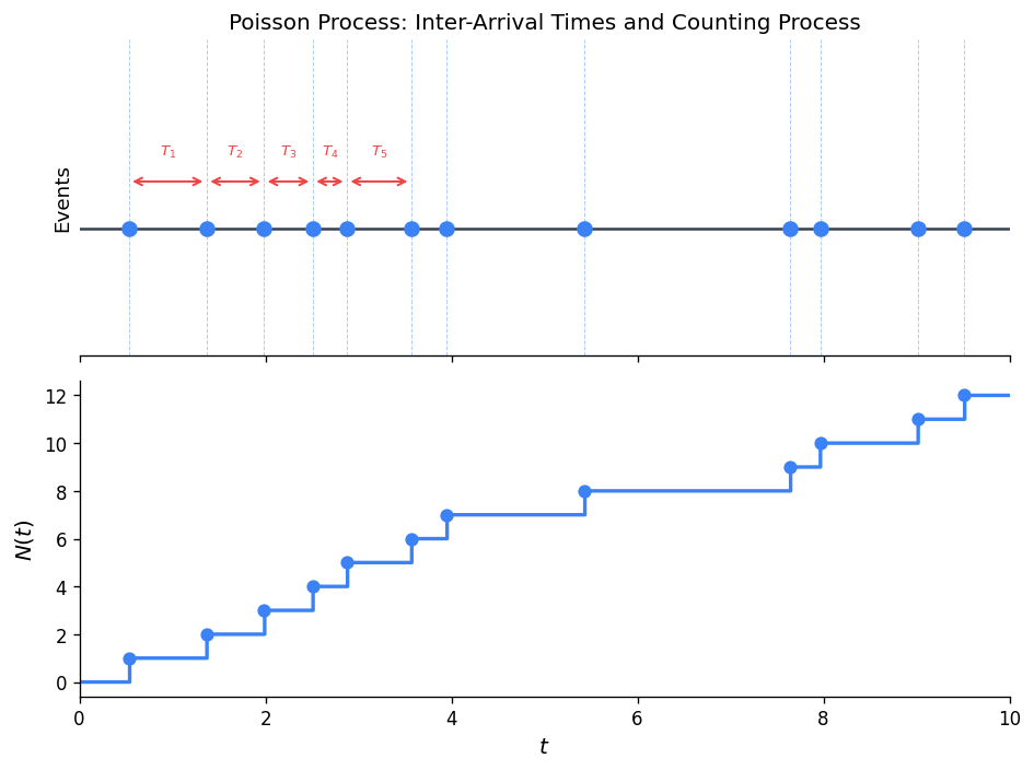
Inter-Arrival and Arrival Times

Define:

• Inter-arrival times \(T_n = S_n - S_{n-1}\), where \(S_n\) is the time of the \(n\)-th event and \(S_0 = 0\).
• Arrival time of the \(n\)-th event: \(S_n = T_1 + T_2 + \cdots + T_n\).

Theorem 4.4. The inter-arrival times \(T_1, T_2, \ldots\) of a Poisson process with rate \(\lambda\) are iid \(\text{Exp}(\lambda)\) random variables.

Proof. The distribution of \(N(t)\) gives \(P(T_1 > t) = P(N(t) = 0) = e^{-\lambda t}\), so \(T_1 \sim \text{Exp}(\lambda)\). By the stationary and independent increments properties, the same holds for all subsequent inter-arrival times, and they are mutually independent.

Corollary. The \(n\)-th arrival time \(S_n = T_1 + \cdots + T_n\) has an Erlang\((n, \lambda)\) distribution.

4.3 Further Properties of the Poisson Process

Conditional Distribution of Arrivals

Theorem 4.5. Given \(N(t) = n\), the conditional distribution of \(N(s)\) (for \(s < t\)) is

\[ N(s) \mid N(t) = n \;\sim\; \text{Binomial}\!\left(n,\, \frac{s}{t}\right). \]

Proof. For \(m \leq n\):

\[ P(N(s) = m \mid N(t) = n) = \frac{P(N(s) = m)\,P(N(t) - N(s) = n-m)}{P(N(t) = n)}. \]

Using the Poisson PMFs and the independent increments property, after simplification (the exponential terms cancel), one obtains the Binomial PMF with parameters \(n\) and \(s/t\).

Conditional Distribution of Individual Arrival Times

Theorem 4.5 tells us about the count \(N(s)\) given \(N(t)=n\). A deeper question is: given that exactly one or \(n\) arrivals occurred in \([0,t]\), where in the interval did they occur? The next two theorems answer this.

Proof. Let \(G(s) = P(S_1 \leq s \mid N(t) = 1)\) for \(0 \leq s \leq t\). Applying the definition of conditional probability and the independent increments property:

\[ G(s) = \frac{P(S_1 \leq s,\; N(t) = 1)}{P(N(t) = 1)} = \frac{P(N(s) = 1)\,P(N(t) - N(s) = 0)}{P(N(t) = 1)}. \]

Substituting the Poisson PMF (with means \(\lambda s\), \(\lambda(t-s)\), and \(\lambda t\) respectively):

\[ G(s) = \frac{(\lambda s\, e^{-\lambda s})(e^{-\lambda(t-s)})}{\lambda t\, e^{-\lambda t}} = \frac{\lambda s\, e^{-\lambda t}}{\lambda t\, e^{-\lambda t}} = \frac{s}{t}. \]

Since \(s/t\) is the CDF of \(\text{Uniform}(0,t)\), the result follows. \(\square\)

Intuition. The result says that, conditional on exactly one event occurring in \([0,t]\), the event time is uniformly scattered throughout the interval — the Poisson process has no preferred location.

Order Statistics Background

To state the generalisation, we need a brief introduction to order statistics.

Joint PDF of order statistics. The joint PDF of \((Y_{(1)}, Y_{(2)}, \ldots, Y_{(n)})\) is

\[ g(y_1, y_2, \ldots, y_n) = n!\, f(y_1)\, f(y_2) \cdots f(y_n), \qquad 0 < y_1 < y_2 < \cdots < y_n. \]

The factor \(n!\) accounts for the number of ways to assign \(n\) unordered observations to the \(n\) ordered slots.

Uniform case. If \(Y_i \sim \text{Uniform}(0,t)\), then \(f(y) = 1/t\) and the joint PDF simplifies to

\[ g(y_1, \ldots, y_n) = \frac{n!}{t^n}, \qquad 0 < y_1 < y_2 < \cdots < y_n < t. \]

The marginal PDF of the \(i\)-th order statistic \(Y_{(i)}\) is

\[ g_{(i)}(y) = \frac{n!}{(i-1)!\,(n-i)!} \cdot \frac{y^{i-1}(t-y)^{n-i}}{t^n}, \qquad 0 < y < t, \]

which is a scaled Beta distribution.

Proof. Fix \(0 < s_1 < s_2 < \cdots < s_n < t\). By the independent increments property, the events that exactly one arrival falls in each of the intervals \((0,s_1]\), \((s_1,s_2]\), \ldots, \((s_{n-1},s_n]\), and zero arrivals fall in \((s_n,t]\), are mutually independent. Therefore:

\[ P\!\left(\bigcap_{k=1}^n \{N(s_{k-1}, s_k) = 1\} \cap \{N(s_n, t) = 0\}\right) = \prod_{k=1}^n \Bigl[\lambda(s_k - s_{k-1})\, e^{-\lambda(s_k - s_{k-1})}\Bigr] \cdot e^{-\lambda(t-s_n)}, \]

where \(s_0 = 0\). The product of exponentials collapses to \(e^{-\lambda t}\) (since the exponents sum to \(\lambda t\)), giving:

\[ = \lambda^n \prod_{k=1}^n (s_k - s_{k-1}) \cdot e^{-\lambda t}. \]

Dividing by \(P(N(t) = n) = (\lambda t)^n e^{-\lambda t}/n!\) and differentiating with respect to each \(s_k\) yields the conditional joint PDF:

\[ f(s_1, \ldots, s_n \mid N(t) = n) = \frac{\lambda^n\, e^{-\lambda t}}{(\lambda t)^n e^{-\lambda t}/n!} \cdot \frac{\partial^n}{\partial s_1 \cdots \partial s_n}\!\left[\prod_{k=1}^n (s_k - s_{k-1})\right] = \frac{n!}{t^n}. \quad \square \]

Remark. The remarkable conclusion is that, given \(n\) events have occurred by time \(t\), the event locations are completely uninformative about the Poisson rate \(\lambda\) — they are simply \(n\) i.i.d. uniform points placed on \([0,t]\) and then sorted. Theorem 4.6 is the special case \(n = 1\).

Applications of Theorem 4.7

Example 4.A (Discounted total revenue). Cars arrive to a toll bridge according to a Poisson process with rate \(\lambda\). Each car pays $1 upon arrival. Let \(\alpha > 0\) be a continuous discount rate, so the present value at time 0 of a payment made at time \(s\) is \(e^{-\alpha s}\). Define the total discounted revenue by time \(t\):

\[ T = \sum_{i=1}^{N(t)} e^{-\alpha S_i}. \]

Finding \(E[T]\). Condition on \(N(t) = n\). By Theorem 4.7, the \(S_i\) given \(N(t)=n\) are distributed as \(n\) i.i.d. \(\text{Uniform}(0,t)\) variables (up to ordering). Since \(\sum e^{-\alpha s_i}\) is invariant under permutation:

\[ E[T \mid N(t) = n] = n\, E[e^{-\alpha U}], \qquad U \sim \text{Uniform}(0,t). \]

Computing the expectation: \(E[e^{-\alpha U}] = \int_0^t e^{-\alpha u}/t\, du = (1 - e^{-\alpha t})/(\alpha t)\). By the law of total expectation:

\[ \boxed{E[T] = E[N(t)]\, E[e^{-\alpha U}] = \lambda t \cdot \frac{1 - e^{-\alpha t}}{\alpha t} = \frac{\lambda(1 - e^{-\alpha t})}{\alpha}.} \]

Finding \(\text{Var}(T)\). Let \(B = (1-e^{-\alpha t})/(\alpha t)\) and \(D = (1-e^{-2\alpha t})/(2\alpha t)\). Since \(Y_1,\ldots,Y_n\) are i.i.d. Uniform\((0,t)\):

\[ \text{Var}(T \mid N(t) = n) = n\, \text{Var}(e^{-\alpha U}) = n(D - B^2). \]

Applying the conditional variance formula (Theorem 2.3) and using \(E[N(t)] = \text{Var}(N(t)) = \lambda t\):

\[ \text{Var}(T) = E[N(t)](D - B^2) + B^2\,\text{Var}(N(t)) = \lambda t\, D = \frac{\lambda(1-e^{-2\alpha t})}{2\alpha}. \]

Example 4.B (Satellite launches). Satellites are launched according to a Poisson process at rate \(\lambda = 3\) per year. Given that exactly 2 launches occurred in the past year (\(t = 1\)), find the probability that the first launch was within the first 5 months and the second launch was before the final 2 months.

In terms of years: we want \(P(S_1 \leq 5/12,\; S_2 \leq 5/6 \mid N(1) = 2)\).

By Theorem 4.7, \((S_1, S_2) \mid N(1) = 2\) has joint PDF \(g(s_1, s_2) = 2!/1^2 = 2\) on \(0 < s_1 < s_2 < 1\). Integrating over the relevant region:

\[ P(S_1 \leq {\textstyle\tfrac{5}{12}},\; S_2 \leq {\textstyle\tfrac{5}{6}} \mid N(1) = 2) = \int_0^{5/12} \int_{s_1}^{5/6} 2\, ds_2\, ds_1 = \int_0^{5/12} 2\!\left(\tfrac{5}{6} - s_1\right) ds_1. \]

Evaluating: \(= 2\!\left[\tfrac{5}{6}s_1 - \tfrac{s_1^2}{2}\right]_0^{5/12} = 2\!\left(\tfrac{25}{72} - \tfrac{25}{288}\right) = 2 \cdot \tfrac{75}{288} = \dfrac{25}{48} \approx 0.521\).

Superposition and Thinning

Superposition. If \(N_1(t) \sim \text{Poisson}(\lambda_1)\) and \(N_2(t) \sim \text{Poisson}(\lambda_2)\) are independent, then \(N_1(t) + N_2(t) \sim \text{Poisson}(\lambda_1 + \lambda_2)\).

Thinning. If each event of a Poisson\((\lambda)\) process is independently classified as Type1 (probability \(p\)) or Type2 (probability \(1-p\)), then the Type1 events form a Poisson\((\lambda p)\) process and the Type2 events form a Poisson\((\lambda(1-p))\) process, and the two are independent.

Comparison of Two Poisson Processes

Given two independent Poisson processes with arrival times \(S_n^{(1)}\) and \(S_n^{(2)}\) (Erlang-\(n\) distributed with rates \(\lambda_1\) and \(\lambda_2\) respectively), the probability that the \(n\)-th event of process 1 occurs before the \(n\)-th event of process 2 can be expressed as a sum of binomial probabilities. This connects back to the result from Chapter 2 about \(P(X < Y)\) for competing exponentials.

4.4 Generalizations of the Poisson Process

4.4.1 The Non-Homogeneous Poisson Process

The standard Poisson process assumes a constant arrival rate \(\lambda\). In many real-world scenarios (customer arrivals, traffic flow, etc.), the rate varies with time.

Theorem 4.8. For a non-homogeneous Poisson process with rate function \(\lambda(t)\), the number of events in the interval \((s_1, s_1+s_2]\) is Poisson with mean

\[ \int_{s_1}^{s_1+s_2} \lambda(\tau)\,d\tau = m(s_1 + s_2) - m(s_1), \]

where \(m(t) = \int_0^t \lambda(\tau)\,d\tau\) is the mean value function.

Proof sketch. Define the MGF \(\phi_u(s_1, s_2) = E[e^{u(N(s_1+s_2) - N(s_1))}]\). Using independent increments, differentiating with respect to \(s_2\) and taking \(h \to 0\) yields the ODE

\[ \frac{\partial}{\partial s_2}\phi_u(s_1, s_2) = \lambda(s_1 + s_2)(e^u - 1)\,\phi_u(s_1, s_2), \]

with initial condition \(\phi_u(s_1, 0) = 1\). The solution is \(\phi_u(s_1, s_2) = \exp\!\bigl[(e^u - 1)\int_{s_1}^{s_1+s_2}\lambda(\tau)\,d\tau\bigr]\), which is the MGF of the stated Poisson distribution.

4.4.2 The Compound Poisson Process

Each “event” of the Poisson process contributes a random “jump” of size \(Y_i\). Using the random sum formulas from Chapter 2:

\[ E[X(t)] = \lambda t\, E[Y_1], \qquad \text{Var}(X(t)) = \lambda t\, E[Y_1^2]. \]

The MGF of \(X(t)\) is

\[ \phi_{X(t)}(u) = \exp\!\bigl\{\lambda t\,(\phi_{Y_1}(u) - 1)\bigr\}. \]

Compound Poisson processes arise throughout insurance mathematics (aggregate claims models), queuing theory, and mathematical finance.

---

Summary and Key Theorems

The following table summarises the major results from each chapter.

Chapter	Key Result	Statement
1	Theorem 1.1	MGF of a sum of independent RVs is the product of the individual MGFs.
2	Theorem 2.2	Law of Total Expectation: \(E[g(X)] = E[E[g(X)\mid Y]]\).
2	Theorem 2.3	Conditional Variance Formula: \(\text{Var}(X) = E[\text{Var}(X\mid Y)] + \text{Var}(E[X\mid Y])\).
3	Chapman–Kolmogorov	\(n\)-step TPM equals \(P^n\); intermediate conditioning gives \(P^{(n)} = P^{(m)} P^{(n-m)}\).
3	Theorem 3.1	Communicating states have the same period.
3	Theorem 3.2	Recurrence/transience is a class property.
3	Theorem 3.3	If \(i \leftrightarrow j\) and \(i\) is recurrent, then \(f_{ij} = 1\).
3	Theorem 3.4	Finite irreducible chain is recurrent.
3	Theorem 3.5	A recurrent class is closed: \(p_{ij}^{(k)} = 0\) for all \(k\) if \(i\) is recurrent and \(i \not\leftrightarrow j\).
3	Basic Limit Theorem	Irreducible, positive recurrent, aperiodic chain: \(\lim_{n\to\infty} p_{ij}^{(n)} = \pi_j = 1/m_j\), independent of \(i\).
3	Theorem 3.7	Finite irreducible aperiodic chain with doubly stochastic TPM: \(\pi_j = 1/N\).
3	Absorbing chains	Absorption probabilities \(\mathbf{U} = (I-Q)^{-1}R\); mean absorption times \(\mathbf{w} = (I-Q)^{-1}\mathbf{1}\).
4	Theorem 4.1 (Min of exponentials)	Min of independent exponentials is exponential with rate = sum of rates.
4	Memoryless uniqueness	Exponential is the unique continuous memoryless distribution.
4	Theorem 4.4	Inter-arrival times of a Poisson process are iid \(\text{Exp}(\lambda)\).
4	Theorem 4.5	Given \(N(t)=n\), the earlier count \(N(s)\) is \(\text{Binomial}(n, s/t)\).
4	Theorem 4.6	Given \(N(t)=1\), the first arrival time \(S_1 \sim \text{Uniform}(0,t)\).
4	Theorem 4.7	Given \(N(t)=n\), the joint distribution of \((S_1,\ldots,S_n)\) equals that of \(n\) order statistics from i.i.d. \(\text{Uniform}(0,t)\); conditional joint PDF \(= n!/t^n\).
4	Theorem 4.8	Non-homogeneous Poisson process: events in \((s_1, s_1+s_2]\) are Poisson with mean \(\int_{s_1}^{s_1+s_2}\lambda(\tau)d\tau\).

---

Appendix: Notation Reference

Symbol	Meaning
\(P(A)\)	Probability of event \(A\)
\(P(A \mid B)\)	Conditional probability of \(A\) given \(B\)
\(E[X]\), \(\mu\)	Expected value (mean) of \(X\)
\(\text{Var}(X)\), \(\sigma^2\)	Variance of \(X\)
\(\phi_X(t)\)	MGF of \(X\): \(E[e^{tX}]\)
\(F(x)\)	CDF of \(X\): \(P(X \leq x)\)
\(\bar{F}(x)\)	Tail probability: \(P(X > x)\)
\(p_{ij}^{(n)}\)	\(n\)-step transition probability from state \(i\) to state \(j\)
\(f_{ij}^{(n)}\)	First-passage probability from \(i\) to \(j\) at step \(n\)
\(d(i)\)	Period of state \(i\)
\(\boldsymbol{\pi}\)	Stationary distribution of a Markov chain
\(N(t)\)	Counting process at time \(t\)
\(\lambda\)	Rate parameter (exponential / Poisson)
\(S_n\)	Arrival time of the \(n\)-th event in a Poisson process
\(T_n\)	\(n\)-th inter-arrival time