Unit 1: The Breakdown of Classical Physics

Physics at the close of the nineteenth century rested on two seemingly complete pillars: particles obeying Newtonian mechanics and electromagnetic waves governed by Maxwell’s equations. Point particles could be described entirely by position and momentum, with an associated kinetic and potential energy, and the laws of collision and conservation applied without exception. Waves, on the other hand, spread continuously through space, carried energy distributed over their entire extent, and produced interference when superimposed. Nothing in classical theory suggested that these two descriptions would ever need to overlap.

Then a series of experiments shattered that boundary. Blackbody radiation revealed that light energy comes in discrete packets. The photoelectric effect showed that electromagnetic waves behave like particles when they knock electrons off metals. The Compton effect demonstrated that photons carry momentum and obey the same conservation laws as billiard balls. And the Davisson-Germer experiment proved the converse — that particles like electrons produce diffraction patterns, behaving unmistakably like waves. Taken together, these results demanded an entirely new framework: quantum mechanics.

Key constants:

• Planck’s constant: \(h = 6.626 \times 10^{-34}\ \mathrm{J \cdot s}\)
• Reduced Planck’s constant: \(\hbar = h / 2\pi = 1.0546 \times 10^{-34}\ \mathrm{J \cdot s}\)
• The unit of energy is the electron-volt: \(1\ \mathrm{eV} = 1.6 \times 10^{-19}\ \mathrm{J}\)

---

The Photoelectric Effect

Experimental Observations

When light strikes a metal surface, electrons are ejected and collected at an opposing plate, producing a measurable current. Classical wave theory predicts that any frequency of light should liberate electrons if the intensity is high enough, that brighter light should eject faster electrons, and that there should be a time delay for weak sources as the electrons gradually absorb enough energy to escape. All three predictions fail spectacularly:

• There is a sharp cutoff frequency \(f_0\) below which no current flows, regardless of intensity.
• Even the faintest light above \(f_0\) produces an instantaneous current — no delay whatsoever.
• Increasing intensity increases the number of ejected electrons but does not change their maximum kinetic energy.

If an external voltage \(V\) is applied against the electron flow, the current ceases at a stopping voltage \(V_0\) that depends on frequency but not on intensity. The cutoff frequency is thus a function of the applied voltage: \(f_0(V)\).

Einstein’s Explanation (1905)

Einstein resolved these puzzles with two radical postulates: light comes in quantized packets called photons, and each photon of frequency \(f\) carries energy

\[ E_f = hf \]

For visible light with \(f \approx 10^{15}\ \mathrm{Hz}\), this gives \(E_f \approx 10^{-19}\ \mathrm{J} \sim 1\ \mathrm{eV}\).

The mechanism is elegantly simple: one photon interacts with one electron. The photon is absorbed completely, transferring its energy to the electron. The electron uses part of this energy to overcome the binding potential of the metal — the work function \(W\) — and the remainder becomes kinetic energy:

\[ hf = W + E_k \]

The cutoff frequency satisfies \(hf_0 = W\), giving \(f_0 = W/h\). If \(f < f_0\), no single photon has enough energy to liberate an electron, and no current flows regardless of intensity. Even if an electron absorbs a sub-threshold photon, its energy dissipates through collisions long before a second photon arrives. With an applied stopping voltage, energy conservation gives:

\[ V_0 = \frac{hf - W}{e} \]

where \(e\) is the electron charge. This linear relationship between stopping voltage and frequency was confirmed experimentally by Millikan in 1916, providing one of the earliest quantitative verifications of the quantum hypothesis.

---

The Compton Effect

Having established that light carries quantized energy, it is natural to ask whether photons also carry momentum. The Compton effect (1923) answers this decisively.

Classical Expectation

In classical electromagnetic theory, light scattered by charged particles undergoes Rayleigh scattering: the oscillating electric field of the incoming wave sets the charges in the target vibrating at the same frequency, and these accelerating charges radiate at that same frequency in all directions. The intensity of Rayleigh scattering scales as \(f^4\) — which is why the sky is blue — but crucially, the frequency of the scattered light is unchanged.

The Quantum Result

When Arthur Compton directed X-rays at graphite targets, he observed that the scattered X-rays at an angle \(\theta\) had a different wavelength from the incident beam, with the shift depending on the scattering angle. This frequency change cannot be explained by classical wave theory.

The quantum explanation treats the interaction as a billiard-ball collision between a photon and a loosely bound electron. The photon has momentum:

\[ p_f = \frac{hf}{c} = \frac{h}{\lambda} \]

Applying conservation of relativistic energy and momentum to the photon-electron collision yields the Compton scattering formula:

\[ \Delta\lambda = \frac{h}{m_e c}(1 - \cos\theta) = \lambda_C(1 - \cos\theta) \]

where \(\lambda_C = h/(m_e c) \approx 2.43 \times 10^{-12}\ \mathrm{m}\) is the Compton wavelength of the electron. The shift is maximal for backscattering (\(\theta = \pi\), giving \(\Delta\lambda = 2\lambda_C\)) and zero for forward scattering. The Compton effect is negligible at optical wavelengths (where \(\Delta\lambda \ll \lambda\)) but dramatic in the X-ray regime, providing irrefutable evidence that photons carry momentum exactly as Einstein’s quantum picture demands.

---

The De Broglie Hypothesis and the Davisson-Germer Experiment

De Broglie’s Postulate (1924)

The photoelectric and Compton effects proved that waves can behave like particles. Louis de Broglie made the audacious leap in the other direction: if the photon momentum relation \(p = h/\lambda\) contains nothing specific to light, perhaps all matter has an associated wavelength. His postulate assigns to every particle of momentum \(p\) a de Broglie wavelength:

\[ \lambda = \frac{h}{p} \]

For macroscopic objects this wavelength is absurdly small — a tennis ball at 50 m/s has \(\lambda \sim 10^{-34}\ \mathrm{m}\) — but for electrons accelerated through modest voltages, \(\lambda\) falls in the range of atomic spacings, making wave-like effects observable.

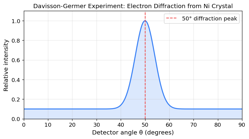
The Davisson-Germer Experiment (1927)

The experimental confirmation came from Clinton Davisson and Lester Germer, who directed a beam of electrons at a nickel crystal. The crystal lattice acts as a Bragg grating: planes of atoms separated by distance \(d\) reflect waves, and constructive interference occurs when the path length difference satisfies the Bragg condition:

\[ n\lambda = 2d\sin\phi \]

where \(\phi\) is the angle of incidence and \(n\) is a positive integer. Davisson and Germer observed sharp diffraction maxima at exactly the angles predicted by the Bragg condition using de Broglie’s wavelength for the electrons. This was the definitive proof that particles exhibit wave-like properties such as diffraction and interference — and it earned de Broglie the 1929 Nobel Prize in Physics.

The stage was now set: waves behave like particles (photoelectric, Compton), and particles behave like waves (Davisson-Germer, double slit). The task of quantum mechanics is to provide a unified framework encompassing both.

---

Unit 2: Foundations of Quantum Mechanics

The central theme of this course is the Stern-Gerlach experiment, which exposes all the essential features of quantum mechanics in a compact, tangible setting. We begin with spin, a fundamentally quantum property with no classical analogue, before building the general formalism and applying it to the Schrödinger equation and wave mechanics.

The Stern-Gerlach Experiment I

The Physical Setup

A magnetic field gradient exerts a force on a magnetic moment \(\boldsymbol{\mu}\):

\[ \mathbf{F} = -\nabla U = \nabla(\boldsymbol{\mu} \cdot \mathbf{B}) \]

A magnetic moment has two contributions from orbital and intrinsic (spin) angular momenta:

\[ \boldsymbol{\mu}_{\mathrm{total}} = \boldsymbol{\mu}_{\mathrm{orbital}} + \boldsymbol{\mu}_{\mathrm{spin}}, \quad \boldsymbol{\mu}_{\mathrm{orbital}} = \frac{q}{2m}\mathbf{L}, \quad \boldsymbol{\mu}_{\mathrm{spin}} = g\frac{q}{2m}\mathbf{S} \]

where \(g \approx 2\) for an electron spin. Stern and Gerlach sent a beam of silver atoms through an inhomogeneous magnetic field. Silver has the electronic configuration \(1s^2 2s^2 2p^6 3s^2 3p^6 4s^2 3d^{10} 4p^6 4d^{10} 5s^1\). All filled shells have zero total orbital angular momentum, leaving a single unpaired \(5s\) electron (which has zero orbital angular momentum), so the magnetic moment is purely from spin.

The force on a spin in the gradient is:

\[ F_z = (\boldsymbol{\mu} \cdot \hat{z})\frac{\partial B_z}{\partial z} = |\boldsymbol{\mu}|\cos\theta\,\frac{\partial B_z}{\partial z} \]

Quantization of Spin

Classically, one would expect a continuous smear of deflection angles. Instead, Stern and Gerlach observed two discrete spots, showing that the angular momentum is quantized. A measurement of spin along any axis yields only two values:

\[ S_z = \pm\frac{\hbar}{2} \]

Particles with \(|S_z| = \hbar/2\) are called spin-\(\frac{1}{2}\) particles.

The Quantum State Vector (Postulate 1)

Using Dirac notation, \(|{+}\rangle\) denotes the spin-up state (deflected upward) and \(|{-}\rangle\) denotes spin-down. The general state is a linear superposition:

\[ |\psi\rangle = a|{+}\rangle + b|{-}\rangle \]

where \(a\) and \(b\) are complex coefficients. You may also see \(|{+}\rangle = |{+}\hbar/2\rangle = |\uparrow\rangle = |{+}\hat{z}\rangle\).

Three Stern-Gerlach Experiments

Experiment 1: Prepare \(|{+}\rangle\) in Analyzer 1, measure again with Analyzer 2 along the same \(z\)-axis. Result: 100% probability of measuring \(|{+}\rangle\). Measurement of a definite eigenstate returns a definite result.

Experiment 2: Prepare \(|{+}\rangle_z\), then measure along the \(x\)-axis. Result: 50%/50% probability of \(|{+}\rangle_x\) or \(|{-}\rangle_x\). The state \(|{+}\rangle_z\) is a superposition of the \(x\)-eigenstates.

Experiment 3: Prepare \(|{+}\rangle_z\), measure \(S_x\) to obtain \(|{+}\rangle_x\), then measure \(S_z\) again. Result: 50%/50% for \(|{\pm}\rangle_z\). The measurement of \(S_x\) disturbs our knowledge of \(S_z\). Measurements of orthogonal spin components are incompatible—measuring one destroys information about the other. The order of measurements matters.

---

The Stern-Gerlach Experiment II — Quantum Interference

Experiment 4: The Absence of “Which-Path” Information

In Experiment 4, we combine both output ports of the \(x\)-analyzer (Analyzer 2) and feed them into Analyzer 3 (oriented along \(z\)) without measuring which port the spin exited from. Classically, based on Experiments 3A and 3B, we would expect 50% probability to exit the \(|{-}\rangle\) port of A3. But the quantum result is that 100% of spins exit the \(|{+}\rangle\) port of A3, and 0% exit \(|{-}\rangle\).

It is as if Analyzer 2 was not there. By not observing which path the spin takes, the two paths interfere. This is analogous to Young’s double-slit experiment with light.

Young’s Double-Slit Interference

With half the incident amplitude exiting each slit, the amplitude at point P on a screen is:

\[ A(P) = \frac{A}{2}\left(e^{ikr_1} + e^{ikr_2}\right)e^{-i\omega t} \]

The intensity is proportional to the probability of detecting a photon:

\[ I(P) = \left(\frac{A}{2}\right)^2\left[1 + \cos(k[r_1 - r_2])\right] \]

For slit separation \(h\) and screen distance \(l\):

\[ r_1 - r_2 \approx \frac{hx}{l}, \qquad I(P) = \left(\frac{A}{2}\right)^2\left[1 + \cos\!\left(\frac{2\pi h}{\lambda l}x\right)\right] \]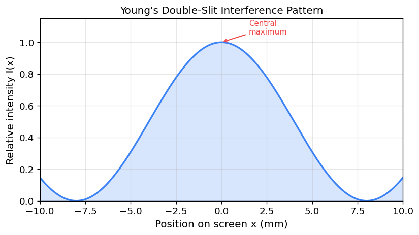

Single-Particle Interference and Probability Amplitudes

The key distinction between classical and quantum probability:

\[ P_{\mathrm{classical}} = |a_1 e^{i\phi_1}|^2 + |a_2 e^{i\phi_2}|^2 = a_1^2 + a_2^2 \]\[ P_{\mathrm{quantum}} = |a_1 e^{i\phi_1} + a_2 e^{i\phi_2}|^2 = a_1^2 + a_2^2 + 2a_1 a_2\cos(\phi_1 - \phi_2) \]

The cross-term \(2a_1 a_2\cos(\phi_1 - \phi_2)\) is the interference term. If you place a detector to determine which slit a photon passes through, the interference disappears and you recover classical probabilities. The act of observation collapses the wavefunction to a definite path, destroying the superposition.

---

Quantum State Vectors and Hilbert Space

Hilbert Space

The ket \(|\psi\rangle\) belongs to a Hilbert space: a complete, complex, inner-product vector space that generalizes Euclidean space. For a spin-\(\frac{1}{2}\) particle, the Hilbert space is 2-dimensional, spanned by \(|{+}\rangle\) and \(|{-}\rangle\). Any state can be written:

\[ |\psi\rangle = a|{+}\rangle + b|{-}\rangle \]

Inner Product and Bras

The bra \(\langle\psi|\) is the conjugate transpose (Hermitian transpose) of \(|\psi\rangle\):

\[ \langle\psi| = (|\psi\rangle)^\dagger = a^*\langle{+}| + b^*\langle{-}| \]

The inner product \(\langle\phi|\psi\rangle\) measures the projection of \(|\phi\rangle\) onto \(|\psi\rangle\). The basis vectors satisfy:

\[ \langle{+}|{+}\rangle = \langle{-}|{-}\rangle = 1 \quad (\text{unit norm}), \qquad \langle{+}|{-}\rangle = \langle{-}|{+}\rangle = 0 \quad (\text{orthogonality}) \]

The probability amplitudes are:

\[ a = \langle{+}|\psi\rangle, \qquad b = \langle{-}|\psi\rangle \]

Normalization

Since there are only two possible outcomes, we require \(P_+ + P_- = 1\):

\[ |a|^2 + |b|^2 = 1 \quad \Longleftrightarrow \quad \langle\psi|\psi\rangle = 1 \]

The normalization constant \(C\) for a state \(|\psi\rangle = 3|{+}\rangle + 2i|{-}\rangle\) is \(C = 1/\sqrt{13}\), giving:

\[ |\psi\rangle_N = \frac{1}{\sqrt{13}}\left(3|{+}\rangle + 2i|{-}\rangle\right) \]

Important: An overall phase factor \(e^{i\theta}\) does not change measurement probabilities, since \(|e^{i\theta}\langle a|\psi\rangle|^2 = |\langle a|\psi\rangle|^2\). We can always choose the overall phase to be real and positive.

Matrix Notation

\[ |{+}\rangle = \begin{pmatrix}1\\0\end{pmatrix}, \quad |{-}\rangle = \begin{pmatrix}0\\1\end{pmatrix}, \quad |\psi\rangle = \begin{pmatrix}a\\b\end{pmatrix}, \quad \langle\psi| = \begin{pmatrix}a^* & b^*\end{pmatrix} \]

---

Representation and Change of Basis

Eigenstates of \(S_x\)

The eigenstates of \(S_x\) can be expressed in the \(S_z\) basis. From measurement outcomes (50%/50% probability for all four combinations), we know \(|a|^2 = |b|^2 = 1/2\). Applying normalization and orthogonality conditions with the phase convention (coefficient of \(|{+}\rangle\) real and positive):

\[ |{+}\rangle_x = \frac{1}{\sqrt{2}}\left(|{+}\rangle + |{-}\rangle\right), \qquad |{-}\rangle_x = \frac{1}{\sqrt{2}}\left(|{+}\rangle - |{-}\rangle\right) \]

Eigenstates of \(S_y\)

Using additional measurement constraints (probability 1/2 when measuring \(S_x\) on eigenstates of \(S_y\), and orthogonality):

\[ |{+}\rangle_y = \frac{1}{\sqrt{2}}\left(|{+}\rangle + i|{-}\rangle\right), \qquad |{-}\rangle_y = \frac{1}{\sqrt{2}}\left(|{+}\rangle - i|{-}\rangle\right) \]

Change of Basis via Transformation Matrix

Given two complete bases \(\{|a\rangle\}\) and \(\{|b\rangle\}\), the transformation matrix \(U\) with elements \(U_{mn} = \langle b_m|a_n\rangle\) converts the representation of any state \(|\psi\rangle\) from the \(a\)-basis to the \(b\)-basis:

\[ |\psi\rangle_b = U|\psi\rangle_a \]

The transformation matrix is unitary: \(UU^\dagger = U^\dagger U = \mathbf{1}\), \(U^\dagger = U^{-1}\). Unitarity ensures that inner products (and hence probabilities) are preserved.

For the transformation from \(S_z\) to \(S_x\) eigenbasis:

\[ U_{z\to x} = \frac{1}{\sqrt{2}}\begin{pmatrix}1 & 1 \\ 1 & -1\end{pmatrix} \]

---

Operators and the Spin Angular Momentum Matrices

Postulates 2 and 3

Physical observables are represented by Hermitian matrices: \(\hat{A} = \hat{A}^\dagger\), where \((\hat{A}^\dagger)_{ij} = A^*_{ji}\). Key properties:

1. Real eigenvalues: Hermitian matrices guarantee that measurement outcomes are real.
2. Orthogonal eigenvectors: Eigenvectors with distinct eigenvalues are orthonormal.
3. Diagonal in eigenbasis: \(A_{nm} = \langle a_n|\hat{A}|a_m\rangle = a_n\,\delta_{nm}\).

Pauli Matrices and Spin Operators

The three components of the spin-\(\frac{1}{2}\) angular momentum operator in the \(S_z\) eigenbasis are:

\[ S_z = \frac{\hbar}{2}\begin{pmatrix}1 & 0 \\ 0 & -1\end{pmatrix}, \qquad S_x = \frac{\hbar}{2}\begin{pmatrix}0 & 1 \\ 1 & 0\end{pmatrix}, \qquad S_y = \frac{\hbar}{2}\begin{pmatrix}0 & -i \\ i & 0\end{pmatrix} \]

These are related to the Pauli matrices \(\sigma_i\) by \(S_i = \hbar\sigma_i/2\):

\[ \sigma_x = \begin{pmatrix}0 & 1\\ 1 & 0\end{pmatrix}, \qquad \sigma_y = \begin{pmatrix}0 & -i\\ i & 0\end{pmatrix}, \qquad \sigma_z = \begin{pmatrix}1 & 0\\ 0 & -1\end{pmatrix} \]

Each Pauli matrix squares to the identity: \(\sigma_i^2 = \mathbf{1}\).

---

Projection Operators and Postulate 5

The Projection Operator

The projection operator onto state \(|a_n\rangle\) is:

\[ \hat{P}_n := |a_n\rangle\langle a_n| \]

Its expectation value for state \(|\psi\rangle\) equals the probability:

\[ \langle\psi|\hat{P}_n|\psi\rangle = |\langle a_n|\psi\rangle|^2 = P_n \]

Completeness of projection operators:

\[ \sum_n \hat{P}_n = \sum_n |a_n\rangle\langle a_n| = \mathbf{1} \]

This is an enormously useful relation — inserting it into expressions allows us to freely switch between bases.

Spectral Decomposition

Any observable can be reconstructed from its eigenvalues and projection operators:

\[ \hat{A} = \sum_n a_n |a_n\rangle\langle a_n| \]

Measurement and Wavefunction Collapse

The measurement projects (collapses) the state onto the eigenstate \(|a_n\rangle\). All subsequent measurements with \(\hat{A}\) will yield \(a_n\) with certainty.

Application to S-G Experiment 4: When both ports of the \(x\)-analyzer are combined without observation:

\[ |\psi_2\rangle = \left(|{+}\rangle_x{}_x\langle{+}| + |{-}\rangle_x{}_x\langle{-}|\right)|{+}\rangle = \mathbf{1}|{+}\rangle = |{+}\rangle \]

The completeness relation shows that not observing which path removes the \(x\)-measurement entirely—as if Analyzer 2 was not present. Interference is restored.

---

The Bloch Sphere and Rotation Operators

Arbitrary Spin-\(\frac{1}{2}\) States

The most general normalized spin-\(\frac{1}{2}\) state (up to an overall phase) is:

\[ |\psi_+(θ,\phi)\rangle = \cos\!\left(\frac{\theta}{2}\right)|{+}\rangle + \sin\!\left(\frac{\theta}{2}\right)e^{i\phi}|{-}\rangle \]

The orthogonal state is:

\[ |\psi_-(θ,\phi)\rangle = \sin\!\left(\frac{\theta}{2}\right)|{+}\rangle - \cos\!\left(\frac{\theta}{2}\right)e^{i\phi}|{-}\rangle \]

The angles \(\theta\) and \(\phi\) parameterize the unit sphere — the Bloch sphere — named after Felix Bloch. Every point on the Bloch sphere’s surface represents a distinct spin-\(\frac{1}{2}\) state. The north pole \(\theta=0\) is \(|{+}\rangle\), and the equator (\(\theta=\pi/2\)) contains the \(S_x\) and \(S_y\) eigenstates.

Angular Momentum as Generator of Rotation

The infinitesimal rotation operator about the \(z\)-axis by angle \(d\phi\) is:

\[ \hat{R}_z(d\phi) := \mathbf{1} - \frac{i}{\hbar}\hat{S}_z\,d\phi \]

For a finite rotation by angle \(\phi_0\):

\[ \hat{R}_z(\phi_0) = e^{-i\phi_0\hat{S}_z/\hbar} = \begin{pmatrix}e^{-i\phi_0/2} & 0 \\ 0 & e^{i\phi_0/2}\end{pmatrix} \]

This operator rotates the state \(|\psi_+(θ,\phi)\rangle\) counterclockwise about \(z\) by angle \(\phi_0\):

\[ \hat{R}_z(\phi_0)|\psi_+(θ,\phi)\rangle = e^{-i\phi_0/2}|\psi_+(θ,\phi+\phi_0)\rangle \]

The spinor property: A rotation by \(2\pi\) does not return a spin-\(\frac{1}{2}\) state to itself — it picks up a sign:

\[ \hat{R}_z(2\pi)|\psi_+(θ,\phi)\rangle = e^{-i\pi}|\psi_+(θ,\phi)\rangle = -|\psi_+(θ,\phi)\rangle \]

A rotation by \(4\pi\) is needed to fully recover the original state. This spinor property has no classical analogue.

---

Unit 3: Commutation Relations and the Uncertainty Principle

Commutation Relations for Angular Momentum

The Commutator

The commutator of operators \(\hat{A}\) and \(\hat{B}\) is:

\[ [\hat{A}, \hat{B}] := \hat{A}\hat{B} - \hat{B}\hat{A} \]

Non-commutativity implies that the order of measurements matters. This is directly linked to the Stern-Gerlach observations.

Fundamental Angular Momentum Commutation Relations

By studying infinitesimal rotations in 3D Euclidean space and their analogue in the spin-\(\frac{1}{2}\) Hilbert space, we derive:

\[ [S_x, S_y] = i\hbar S_z, \qquad [S_z, S_x] = i\hbar S_y, \qquad [S_y, S_z] = i\hbar S_x \]

In compact form using the Levi-Civita symbol \(\varepsilon_{ijk}\):

\[ [S_i, S_j] = i\hbar\,\varepsilon_{ijk}\,S_k \]

where \(\varepsilon_{123} = \varepsilon_{231} = \varepsilon_{312} = +1\) and \(\varepsilon_{132} = \varepsilon_{213} = \varepsilon_{321} = -1\). This follows because angular momentum generates rotations, and rotations about different axes do not commute.

---

Expectation Values and RMS Uncertainty

The Expectation Value

The expectation value of observable \(\hat{A}\) for state \(|\psi\rangle\) is:

\[ \langle\hat{A}\rangle = \langle\psi|\hat{A}|\psi\rangle = \sum_n a_n P_n = \sum_n a_n |\langle a_n|\psi\rangle|^2 \]

This is the statistical average of repeated measurements on identically prepared systems (state tomography requires many identical copies, since each measurement collapses the state).

For the states \(|{\pm}\rangle\): \(\langle S_z\rangle = \pm\hbar/2\), but \(\langle S_x\rangle = \langle S_y\rangle = 0\), reflecting the 50%/50% distribution in orthogonal measurements.

RMS Deviation

The root-mean-square (RMS) uncertainty in measurements of \(\hat{A}\) is:

\[ \Delta A = \sqrt{\langle A^2\rangle - \langle A\rangle^2} = \sqrt{\langle(A - \langle A\rangle)^2\rangle} \]

For the states \(|{\pm}\rangle\): \(\Delta S_z = 0\) (definite outcome), but \(\Delta S_x = \Delta S_y = \hbar/2\) (maximal uncertainty in orthogonal components). This can be verified using \(S_x^2 = S_y^2 = S_z^2 = \hbar^2/4 \cdot \mathbf{1}\).

---

The Uncertainty Principle

Statement

Derivation Sketch

1. Cauchy-Schwarz inequality: For any \(|\alpha\rangle\) and \(|\beta\rangle\): \(\langle\alpha|\alpha\rangle\langle\beta|\beta\rangle \geq |\langle\alpha|\beta\rangle|^2\).
2. Set \(|\alpha\rangle = \Delta A|\psi\rangle\) and \(|\beta\rangle = \Delta B|\psi\rangle\), so \(\langle\alpha|\alpha\rangle = \langle(\Delta A)^2\rangle\) and \(\langle\beta|\beta\rangle = \langle(\Delta B)^2\rangle\).
3. Write \(\Delta A\,\Delta B = \frac{1}{2}[A,B] + \frac{1}{2}\{\Delta A,\Delta B\}\).
4. The commutator \([A,B]\) of two Hermitian operators is anti-Hermitian (imaginary expectation value), while the anti-commutator \(\{A,B\}\) is Hermitian (real expectation value). Taking the modulus squared and dropping the anti-commutator term (which only strengthens the inequality) gives the result.

Application to Spin

For the state \(|{+}\rangle\) with \(\langle S_z\rangle = \hbar/2\):

\[ \Delta S_x\,\Delta S_y \geq \frac{1}{2}|\langle[S_x, S_y]\rangle| = \frac{\hbar}{2}|\langle S_z\rangle| = \frac{\hbar^2}{4} \]

Indeed, \(\Delta S_x = \Delta S_y = \hbar/2\), so \(\Delta S_x\,\Delta S_y = \hbar^2/4\). The bound is saturated. We can never simultaneously know all three components of angular momentum. Only the magnitude \(|\mathbf{S}| = \sqrt{3}\,\hbar/2\) is simultaneously definite with any one component.

---

Interaction-Free Measurement: The Elitzur-Vaidman Bomb Tester

One of the most striking consequences of quantum superposition is that it permits interaction-free measurement — detecting the presence of an object without a single photon ever touching it. The Elitzur-Vaidman bomb problem, first proposed in 1993, provides a vivid illustration.

The Setup

Consider a factory that produces bombs fitted with optical fuses so sensitive that a single photon striking the fuse detonates the bomb. Unfortunately, some bombs are defective — their fuses do not work. The challenge is to identify working bombs without detonating them.

Classically this is impossible: any photon that tests the fuse either detonates the bomb (confirming it works) or passes through (leaving us uncertain). Quantum mechanics, however, offers a way out using a Mach-Zehnder interferometer — two 50-50 beam splitters connected by two paths.

Without the Bomb

A photon entering the interferometer from the lower path encounters beam splitter \(B_1\), which creates a superposition of the upper and lower paths. Both paths converge at beam splitter \(B_2\). The beam splitter operators are:

\[ B_1 = \frac{1}{\sqrt{2}}\begin{pmatrix}1 & 1 \\ 1 & -1\end{pmatrix}, \qquad B_2 = \frac{1}{\sqrt{2}}\begin{pmatrix}-1 & 1 \\ 1 & 1\end{pmatrix} \]

The output state is:

\[ |\text{out}\rangle = B_2 B_1 |\text{down}\rangle = |\text{up}\rangle \]

Due to destructive interference in the lower output port, the photon always exits upward and arrives at Detector 1. Detector 2 never clicks.

With a Working Bomb

Now place a working bomb in the upper path. If the photon takes the upper path (probability 1/2), the bomb detonates. If it takes the lower path (probability 1/2), the bomb is untouched — but the superposition is destroyed because the upper path has been blocked. Without interference, the photon at \(B_2\) has equal probability of reaching either detector.

The three outcomes are:

• Bomb explodes (50%): the photon hit the fuse.
• Detector 1 clicks (25%): indistinguishable from a defective bomb — no information gained.
• Detector 2 clicks (25%): this never happens without the bomb. The photon reached Detector 2 without touching the bomb, yet we know with certainty that the bomb is live.

Bomb Status	Explodes	Detector 1	Detector 2
Defective	—	100%	0%
Working	50%	25%	25%

A click at Detector 2 constitutes interaction-free measurement: we have certified a bomb as working using a photon that never interacted with it. The mere possibility of interaction — the bomb’s capacity to absorb a photon on one path — is enough to destroy the interference that would otherwise prevent Detector 2 from firing.

Starting with 70% working bombs, a single pass yields 17.5% certified working bombs (without detonation), 47.5% undetermined, and 35% exploded. By recycling the undetermined bombs through repeated trials, the yield improves further. Remarkably, more sophisticated schemes using the quantum Zeno effect can push the success rate arbitrarily close to 100%.

---

The Quantum Zeno Effect

The quantum Zeno effect demonstrates that sufficiently frequent observation can freeze the evolution of a quantum system, holding it in its initial state indefinitely. The name alludes to Zeno’s paradox of the arrow — if observed at each instant, a moving arrow appears stationary.

Setup

Consider a unitary operator \(U\) that flips a spin from \(|{+}\rangle\) to \(|{-}\rangle\) (implemented, say, by passing the particle through a magnetic field region of appropriate length \(L\)). Now divide this region into \(n\) equal segments, each implementing a partial rotation:

\[ U_{L/n} = \begin{pmatrix}\cos\!\left(\frac{\pi}{2n}\right) & i\sin\!\left(\frac{\pi}{2n}\right) \\ i\sin\!\left(\frac{\pi}{2n}\right) & \cos\!\left(\frac{\pi}{2n}\right)\end{pmatrix} \]

Note that \(U_{L/n}^n = U\): applying all \(n\) partial rotations recovers the full flip. Insert a \(z\)-oriented Stern-Gerlach device after each segment, blocking the \(|{-}\rangle\) component.

Quantitative Analysis

After one segment followed by a measurement, the probability of surviving in the \(|{+}\rangle\) state is:

\[ P_{\text{survive}}^{(1)} = \cos^2\!\left(\frac{\pi}{2n}\right) \]

After all \(n\) segments (each followed by a measurement), the total survival probability is:

\[ P_{\text{survive}}^{(n)} = \cos^{2n}\!\left(\frac{\pi}{2n}\right) \approx 1 - \frac{\pi^2}{4n} \]

where the last approximation uses \(\cos\theta \approx 1 - \theta^2/2\) for small \(\theta\). As \(n \to \infty\), the survival probability approaches 1: all atoms emerge in the \(|{+}\rangle\) state, even though the magnetic field is trying to flip them.

Physical Interpretation

The mechanism is subtle. Each measurement collapses the state back to \(|{+}\rangle\), converting a coherent probability amplitude into a classical probability. Between measurements, the unitary evolution only rotates the state by a small angle \(\pi/(2n)\), so the probability of finding \(|{-}\rangle\) is only \(\sin^2(\pi/2n) \approx \pi^2/(4n^2)\) — quadratically small. Each measurement resets the clock, and the accumulated probability of ever transitioning to \(|{-}\rangle\) scales as \(n \times \pi^2/(4n^2) = \pi^2/(4n) \to 0\).

In essence, frequent measurement interrupts the coherent buildup of the \(|{-}\rangle\) amplitude. The system is perpetually nudged back to its initial state. This is not merely a theoretical curiosity — the quantum Zeno effect has been observed experimentally in trapped ions and has practical implications for quantum error correction and quantum computing, where controlled measurements can suppress unwanted transitions.

---

The Density Operator

Pure and Mixed Ensembles

So far we have described particles in a definite quantum state \(|\psi\rangle\) — a pure state. However, a statistical mixture of different quantum states (a mixed state or mixed ensemble) cannot be described by a single ket. This situation arises whenever we lack complete information about which quantum state a particle is in — for example, the silver atoms exiting an oven in the Stern-Gerlach experiment are in random spin orientations with no phase coherence between them.

The density operator (or density matrix) \(\hat{\rho}\) provides a unified description that handles both pure and mixed situations:

\[ \hat{\rho} = \begin{cases} |\psi\rangle\langle\psi| & \text{pure state} \\[4pt] \displaystyle\sum_k p_k|\psi_k\rangle\langle\psi_k| & \text{mixed state, with } \sum_k p_k = 1 \end{cases} \]

The density operator is always Hermitian (\(\hat{\rho} = \hat{\rho}^\dagger\)), which can be verified directly: \(\rho_{ij}^* = \langle j|\hat{\rho}|i\rangle^* = \langle i|\hat{\rho}^\dagger|j\rangle = \rho_{ji}\).

Formal Properties

Worked Examples

\[ \hat{\rho}_+ = \begin{pmatrix}1\\0\end{pmatrix}\begin{pmatrix}1&0\end{pmatrix} = \begin{pmatrix}1&0\\0&0\end{pmatrix} \]

Expectation of \(S_z\): \(\langle S_z\rangle = \mathrm{Tr}\!\left(S_z\,\hat{\rho}_+\right) = \mathrm{Tr}\!\left(\frac{\hbar}{2}\begin{pmatrix}1&0\\0&-1\end{pmatrix}\begin{pmatrix}1&0\\0&0\end{pmatrix}\right) = \mathrm{Tr}\!\left(\frac{\hbar}{2}\begin{pmatrix}1&0\\0&0\end{pmatrix}\right) = \frac{\hbar}{2}.\)

Expectation of \(S_x\): \(\langle S_x\rangle = \mathrm{Tr}(S_x\,\hat{\rho}_+) = 0\). (Verify: off-diagonal \(S_x\) paired with diagonal \(\hat{\rho}_+\) gives zero trace.)

\[ \hat{\rho}_{\mathrm{mix}} = \frac{1}{2}|{+}\rangle\langle{+}| + \frac{1}{2}|{-}\rangle\langle{-}| = \frac{1}{2}\begin{pmatrix}1&0\\0&1\end{pmatrix} = \frac{\mathbf{1}}{2} \]

Check: \(\mathrm{Tr}(\hat{\rho}^2) = \mathrm{Tr}\!\left(\frac{1}{4}\mathbf{1}\right) = \frac{1}{2} < 1\) — confirming this is mixed. The expectation value \(\langle S_{\hat{n}}\rangle = \mathrm{Tr}(S_{\hat{n}}\,\hat{\rho}_{\mathrm{mix}}) = 0\) for any direction \(\hat{n}\). This is the defining property of a maximally mixed ensemble: no measurement in any direction reveals a preferred orientation.

\[ \hat{\rho} = \frac{3}{4}\begin{pmatrix}1&0\\0&0\end{pmatrix} + \frac{1}{4}\begin{pmatrix}0&0\\0&1\end{pmatrix} = \begin{pmatrix}3/4&0\\0&1/4\end{pmatrix} \]

\(\mathrm{Tr}(\hat{\rho}^2) = (3/4)^2 + (1/4)^2 = 10/16 = 5/8 < 1\) — mixed. \(\langle S_z\rangle = \frac{\hbar}{2}\!\left(\frac{3}{4} - \frac{1}{4}\right) = \frac{\hbar}{4}.\)

The density matrix is the correct language for describing any real experimental ensemble, including those prepared by partial measurements, thermal equilibration, or entanglement with an environment whose degrees of freedom are traced out.

---

Unit 4: Time Evolution

The Hamiltonian and the Schrödinger Equation

Time Evolution Operator

By analogy with rotation (where angular momentum generates spatial rotations) and translation (where linear momentum generates spatial translations), the energy operator — the Hamiltonian \(H\) — generates translation in time.

The infinitesimal time-evolution operator is:

\[ U(t+\delta t, t) = \mathbf{1} - \frac{iH\,\delta t}{\hbar} \]

Time-Independent Hamiltonians

When \(H\) does not depend on time, the energy eigenstates \(|E_n\rangle\) satisfy \(H|E_n\rangle = E_n|E_n\rangle\) and are stationary states: a system that starts in \(|E_n\rangle\) remains in \(|E_n\rangle\) for all time (acquiring only an overall phase).

For a general initial state \(|\psi(0)\rangle = \sum_n c_n|E_n\rangle\), the solution is:

\[ |\psi(t)\rangle = \sum_n c_n\,e^{-iE_n t/\hbar}|E_n\rangle \]

Each energy eigenstate acquires a phase factor \(e^{-iE_n t/\hbar}\). The expectation value of \(H\) is time-independent: \(\langle H\rangle = \sum_n |c_n|^2 E_n\).

Dynamics from Superpositions

For a two-level superposition \(|\psi(0)\rangle = c_1|E_1\rangle + c_2|E_2\rangle\), the probability that the system remains in its initial state oscillates:

\[ |\langle\psi(0)|\psi(t)\rangle|^2 = |c_1|^4 + |c_2|^4 + 2|c_1|^2|c_2|^2\cos\left[(\omega_2 - \omega_1)t\right] \]

with \(\omega_n = E_n/\hbar\). This oscillation frequency \(\omega_{21} = (E_2 - E_1)/\hbar\) is the Bohr frequency corresponding to the energy difference between the levels.

---

The Ammonia Molecule

The ammonia molecule NH\(_3\) is the quantum mechanics course’s flagship two-level system — concrete enough to visualize, rich enough to demonstrate everything the formalism can do. The nitrogen atom can sit at the apex above or below the plane of the three hydrogen atoms, giving two geometrically distinct configurations which we label \(|1\rangle\) (N above the plane) and \(|2\rangle\) (N below). By the symmetry of the molecule, these two configurations have identical energy \(E_0\) in the absence of any coupling.

The Two-State Hamiltonian

Here is the key quantum mechanical insight: the nitrogen atom’s wavefunction does not vanish at the H-plane. It “leaks” through the barrier by quantum tunneling, so the system is not genuinely confined to one side. The correct eigenstates of the Hamiltonian are therefore not \(|1\rangle\) or \(|2\rangle\) individually, but rather their symmetric and antisymmetric combinations.

In the \(\{|1\rangle, |2\rangle\}\) basis, the Hamiltonian matrix is:

\[ H = \begin{pmatrix} \langle 1|H|1\rangle & \langle 1|H|2\rangle \\ \langle 2|H|1\rangle & \langle 2|H|2\rangle \end{pmatrix} = \begin{pmatrix} E_0 & -A \\ -A & E_0 \end{pmatrix} \]

The diagonal elements are \(E_0\) (both configurations have equal energy by symmetry). The off-diagonal element \(-A < 0\) is the tunneling matrix element — it represents the amplitude for the nitrogen atom to tunnel from one side to the other through the potential barrier separating the two configurations.

Diagonalization: Energy Eigenstates

To find the energy eigenvalues, we solve \(\det(H - \lambda\mathbf{1}) = 0\):

\[ (E_0 - \lambda)^2 - A^2 = 0 \implies \lambda = E_0 \pm A \]

The two energy levels are split symmetrically around \(E_0\). The corresponding normalized eigenvectors are the symmetric and antisymmetric combinations:

\[ |I\rangle = \frac{1}{\sqrt{2}}\bigl(|1\rangle + |2\rangle\bigr), \quad E_I = E_0 - A \]\[ |II\rangle = \frac{1}{\sqrt{2}}\bigl(|1\rangle - |2\rangle\bigr), \quad E_{II} = E_0 + A \]

The lower-energy state \(|I\rangle\) is the symmetric (even-parity) combination and the higher-energy state \(|II\rangle\) is the antisymmetric (odd-parity) combination. This energy ordering makes physical sense: the symmetric state has a wavefunction that is non-zero at the barrier peak, “sampling” less of the repulsive region, while the antisymmetric state has a node at the barrier and pays a larger kinetic energy penalty.

Time Evolution and Inversion Oscillation

The two configurations \(|1\rangle\) and \(|2\rangle\) can be re-expressed in terms of the energy eigenstates:

\[ |1\rangle = \frac{1}{\sqrt{2}}\bigl(|I\rangle + |II\rangle\bigr), \qquad |2\rangle = \frac{1}{\sqrt{2}}\bigl(|I\rangle - |II\rangle\bigr) \]

Suppose the nitrogen atom begins above the plane: \(|\psi(0)\rangle = |1\rangle\). Time evolution gives each energy eigenstate a phase factor:

\[ |\psi(t)\rangle = \frac{1}{\sqrt{2}}\bigl(e^{-iE_I t/\hbar}|I\rangle + e^{-iE_{II} t/\hbar}|II\rangle\bigr) \]

The probability of finding the nitrogen atom above the plane at time \(t\) is:

\[ P_1(t) = |\langle 1|\psi(t)\rangle|^2 = \cos^2\!\left(\frac{At}{\hbar}\right) \]

and the probability below:

\[ P_2(t) = |\langle 2|\psi(t)\rangle|^2 = \sin^2\!\left(\frac{At}{\hbar}\right) \]

The nitrogen atom oscillates between the two configurations with angular frequency \(\omega = 2A/\hbar\), or inversion frequency \(\nu = A/(\pi\hbar)\). For ammonia, \(A \approx 3.84 \times 10^{-5}\ \mathrm{eV}\), giving \(\nu \approx 23.87\ \mathrm{GHz}\) — in the microwave range.

Application: The Maser

This inversion frequency is precisely what made ammonia the active medium of the first maser (Microwave Amplification by Stimulated Emission of Radiation), built by Townes and colleagues in 1954. By selecting molecules in the upper energy state \(|II\rangle\) and placing them in a microwave cavity resonant at \(2A/\hbar\), they achieved stimulated emission at the inversion frequency — the working principle that would later be extended to optical frequencies to create the laser. Townes shared the 1964 Nobel Prize in Physics for this work.

---

Spin Precession and Magnetic Resonance

Spin Hamiltonian

A spin-\(\frac{1}{2}\) particle in a magnetic field \(\mathbf{B}\) has the Hamiltonian:

\[ H = -\boldsymbol{\mu}\cdot\mathbf{B} = -\gamma\mathbf{S}\cdot\mathbf{B}, \qquad \gamma = \frac{gq}{2m} \]

For a static field \(\mathbf{B} = B_0\hat{z}\), \(H = -\omega_0 S_z\) with \(\omega_0 = \gamma B_0\). The eigenstates are \(|{\pm}\rangle\) with energies \(\mp\hbar\omega_0/2\).

Larmor Precession

Starting from an arbitrary initial state, the expectation value of the spin vector precesses about \(\hat{z}\) at the Larmor frequency \(\omega_0 = \gamma B_0\):

\[ \langle S_x(t)\rangle = \langle S_x(0)\rangle\cos(\omega_0 t) + \langle S_y(0)\rangle\sin(\omega_0 t) \]

This is Ehrenfest’s theorem in action: the quantum expectation value follows the classical equation of motion.

Magnetic Resonance

Adding a circularly polarized oscillating field perpendicular to \(B_0\):

\[ \mathbf{B}_1(t) = B_1\left[\cos(\omega t)\hat{x} - \sin(\omega t)\hat{y}\right] \]

The full Hamiltonian is \(H(t) = -\omega_0 S_z - \omega_1\left[\cos(\omega t)S_x - \sin(\omega t)S_y\right]\) with \(\omega_1 = \gamma B_1\).

In a rotating frame (transforming away the time-dependence), the effective Hamiltonian becomes time-independent. At resonance (\(\omega = \omega_0\)), the oscillating field drives complete spin-flips between \(|{+}\rangle\) and \(|{-}\rangle\) — the phenomenon of Rabi oscillations, foundational to NMR, MRI, and quantum computing.

The transition probability oscillates as:

\[ P_{+\to -}(t) = \frac{\omega_1^2}{\Omega^2}\sin^2\!\left(\frac{\Omega t}{2}\right), \qquad \Omega = \sqrt{(\omega_0-\omega)^2 + \omega_1^2} \]

At resonance, \(\Omega = \omega_1\) and \(P_{+\to -} = \sin^2(\omega_1 t/2)\), reaching unity at \(t = \pi/\omega_1\) (a \(\pi\)-pulse).

---

Applications of Time Evolution

Constant Energy Shifts

If every energy eigenvalue is shifted by a constant \(\Delta\), so that \(H' = \sum_n (E_n + \Delta)|E_n\rangle\langle E_n|\), the time-evolved state simply acquires an additional global phase:

\[ |\psi'(t)\rangle = e^{-i\Delta t/\hbar}\,|\psi(t)\rangle \]

Since the global phase factor \(e^{-i\Delta t/\hbar}\) cancels in all expectation values and probabilities, a uniform energy shift is physically irrelevant. This is the quantum analogue of the classical freedom to choose the zero of potential energy.

Neutrino Oscillations

Neutrinos are relativistic leptons that interact only via the weak force. Three flavours exist — the electron neutrino \(\nu_e\), the muon neutrino \(\nu_\mu\), and the tau neutrino \(\nu_\tau\) — produced in reactions like:

\[ p \to n + e^+ + \nu_e, \qquad \pi^+ \to \mu^+ + \nu_\mu \]

The three flavour states span a vector space: \(|\psi\rangle = \alpha|\nu_e\rangle + \beta|\nu_\mu\rangle + \gamma|\nu_\tau\rangle\). A deep puzzle emerged when solar neutrino experiments detected only about a third of the predicted electron neutrinos. Quantum mechanics explains this through neutrino oscillations — flavour states are not energy eigenstates.

In the simplified two-flavour case (neglecting \(\nu_\tau\) for solar neutrinos), the flavour eigenstates are related to the mass eigenstates \(|\nu_1\rangle\), \(|\nu_2\rangle\) by a mixing angle \(\theta\):

\[ |\nu_e\rangle = \cos\frac{\theta}{2}\,|\nu_1\rangle + \sin\frac{\theta}{2}\,|\nu_2\rangle, \qquad |\nu_\mu\rangle = \sin\frac{\theta}{2}\,|\nu_1\rangle - \cos\frac{\theta}{2}\,|\nu_2\rangle \]

Since neutrinos interact so weakly, they propagate essentially as free particles with relativistic energies \(E_j = \sqrt{(pc)^2 + (m_j c^2)^2}\). An electron neutrino produced at \(t = 0\) evolves as:

\[ |\psi(t)\rangle = \cos\frac{\theta}{2}\,e^{-iE_1 t/\hbar}|\nu_1\rangle + \sin\frac{\theta}{2}\,e^{-iE_2 t/\hbar}|\nu_2\rangle \]

The probability of detecting a muon neutrino at time \(t\) oscillates:

\[ P(\nu_e \to \nu_\mu) = \sin^2\theta\,\sin^2\!\left(\frac{(E_1 - E_2)t}{2\hbar}\right) \]

Since neutrinos travel at nearly the speed of light, we substitute \(t = L/c\) to express this in terms of distance \(L\) from the source:

\[ P(\nu_e \to \nu_\mu) = \sin^2\theta\,\sin^2\!\left(\frac{(m_1^2 - m_2^2)Lc^3}{4E\hbar}\right) \]

Experimental measurements give \(m_1^2 - m_2^2 \approx 8 \times 10^{-5}\ \mathrm{eV}^2/c^4\) and a mixing angle \(\theta \approx 69°\). This is a beautiful macroscopic manifestation of the quantum superposition principle: a particle created with a definite flavour does not retain that flavour as it propagates, because flavour and mass are described by different bases. The resolution of the solar neutrino problem earned the 2015 Nobel Prize in Physics.

Quantum Clocks

A quantum clock exploits the Bohr frequency of a two-level system to measure time with extraordinary precision. The idea is conceptually identical to a pendulum clock, but with a quantum oscillator replacing the mechanical one.

Consider an atom with ground state \(|g\rangle\) (energy \(E_g\)) and excited state \(|e\rangle\) (energy \(E_e\)). The Hamiltonian is \(H = E_g|g\rangle\langle g| + E_e|e\rangle\langle e|\). Prepare the atom in the equal superposition \(|\psi(0)\rangle = (|e\rangle + |g\rangle)/\sqrt{2}\) by applying a \(\pi/2\)-pulse (a 90° rotation on the Bloch sphere using a resonant field along the \(y\)-axis):

\[ U_{\pi/2} = \frac{1}{\sqrt{2}}\begin{pmatrix}1 & 1 \\ -1 & 1\end{pmatrix} \]

On the Bloch sphere, this places the state vector on the equator. Under free evolution, the Bloch vector precesses around the \(z\)-axis at the Bohr frequency \(\Omega = (E_e - E_g)/\hbar\):

\[ |\psi(t)\rangle = \frac{1}{\sqrt{2}}\left(e^{-iE_e t/\hbar}|e\rangle + e^{-iE_g t/\hbar}|g\rangle\right) \]

After a time interval \(\Delta t\), apply the inverse rotation \(U_{-\pi/2}\) and measure in the \(\{|e\rangle, |g\rangle\}\) basis. The probability of finding the atom in the ground state is:

\[ P(g) = \cos^2\!\left(\frac{\Omega\,\Delta t}{2}\right) \]

By repeating this protocol many times and measuring \(P(g)\), one determines \(\Omega\,\Delta t\) and hence the elapsed time \(\Delta t\). The period of the oscillation is \(T = 2\pi/\Omega\). Modern atomic clocks based on this principle (using the caesium-133 hyperfine transition at 9.192 GHz) define the SI second and achieve fractional uncertainties below \(10^{-16}\) — losing less than one second in 300 million years.

---

The Bloch Vector: General Theory

The Bloch sphere representation introduced earlier can be formalized using the density matrix and Pauli operators. For any spin-\(\frac{1}{2}\) state (pure or mixed), the Bloch vector \(\vec{v}\) is defined by:

\[ \vec{v} = \begin{pmatrix}\langle\sigma_x\rangle \\ \langle\sigma_y\rangle \\ \langle\sigma_z\rangle\end{pmatrix} = \frac{2}{\hbar}\begin{pmatrix}\langle S_x\rangle \\ \langle S_y\rangle \\ \langle S_z\rangle\end{pmatrix} \]

The density matrix can be expressed compactly in terms of the Bloch vector:

\[ \rho = \frac{1}{2}\left(\mathbf{1} + \vec{v}\cdot\vec{\sigma}\right) \]

For a pure state, \(|\vec{v}| = 1\) (the Bloch vector sits on the surface of the unit sphere). For a mixed state, \(|\vec{v}| < 1\) (the vector lies inside the sphere). The completely mixed state has \(\vec{v} = \vec{0}\) and \(\rho = \mathbf{1}/2\).

The expectation value of spin along an arbitrary direction \(\hat{n}\) follows directly:

\[ \langle S_{\hat{n}}\rangle = \frac{\hbar}{2}\,\vec{v}\cdot\hat{n} \]

and the measurement probabilities are:

\[ P(+_{\hat{n}}) = \frac{1}{2}(1 + \vec{v}\cdot\hat{n}), \qquad P(-_{\hat{n}}) = \frac{1}{2}(1 - \vec{v}\cdot\hat{n}) \]

These formulas make the Bloch sphere a powerful tool for visualizing spin dynamics. Under a Hamiltonian \(H = -\omega_0 S_z\), the Bloch vector precesses around \(\hat{z}\) at the Larmor frequency — exactly as described in the magnetic resonance section above.

---

Unit 5: Wave Mechanics in Position Space

Quantum Mechanics in the Position Basis

Extending to Infinite Dimensions

The position operator \(\hat{x}\) acts on position eigenstates:

\[ \hat{x}|x\rangle = x|x\rangle \]

where \(x \in (-\infty, \infty)\). The position eigenvalues form a continuous spectrum. The completeness relation becomes an integral:

\[ \int_{-\infty}^{\infty}|x\rangle\langle x|\,dx = \mathbf{1} \]

The Wavefunction

The wavefunction is defined as the projection of the state \(|\psi\rangle\) onto a position eigenstate:

\[ \psi(x) := \langle x|\psi\rangle \]

It is a complex function of position. The probability density for finding the particle at position \(x\) is:

\[ |\psi(x)|^2 = |\langle x|\psi\rangle|^2 \quad \text{(probability per unit length)} \]

The probability of finding the particle in the region \([x_1, x_2]\) is:

\[ P(x_1, x_2) = \int_{x_1}^{x_2}|\psi(x)|^2\,dx \]

The normalization condition requires:

\[ \langle\psi|\psi\rangle = \int_{-\infty}^{\infty}|\psi(x)|^2\,dx = 1 \]

The Dirac-Delta Function

The inner product of two position eigenstates is:

\[ \langle x|x'\rangle = \delta(x - x') \]

where \(\delta(x - x')\) is the Dirac-delta function, satisfying:

\[ \int_{-\infty}^{\infty}\delta(x - x')\,dx = 1, \qquad \int_{-\infty}^{\infty}\delta(x - x')f(x)\,dx = f(x') \]

This is the continuous analogue of the Kronecker delta for discrete bases.

Operators in Position Space

The action of a function of \(\hat{x}\) on a wavefunction is simple multiplication: \(A(\hat{x})\psi(x) = A(x)\psi(x)\).

---

The Momentum Operator

Momentum as Generator of Translation

The infinitesimal translation operator \(\hat{T}(\Delta x)\) translates states: \(\hat{T}(\Delta x)|x\rangle = |x + \Delta x\rangle\). It must be unitary and have the form:

\[ \hat{T}(\Delta x) = \mathbf{1} - \frac{i\hat{p}\,\Delta x}{\hbar} \]

By computing \(\hat{T}(\Delta x)|\psi\rangle\) two ways (using the translation definition and Taylor-expanding, vs. using the above form), we identify the momentum operator in the position basis:

\[ \hat{p} \;\mapsto\; -i\hbar\frac{d}{dx} \]

Key Results

\[ \langle x|\hat{p}|\psi\rangle = -i\hbar\frac{d\psi(x)}{dx}, \qquad \langle x|\hat{p}^n|\psi\rangle = \left(-i\hbar\right)^n\frac{d^n\psi}{dx^n} \]

Position-Momentum Commutation Relation

The translation operator does not commute with the position operator:

\[ [\hat{x}, \hat{T}(\Delta x)] = \Delta x \]

which leads to the fundamental canonical commutation relation:

\[ [\hat{x}, \hat{p}] = i\hbar \]

This is the origin of the Heisenberg uncertainty principle for position and momentum:

\[ \Delta x\,\Delta p \geq \frac{\hbar}{2} \]

There is no quantum state in which a particle simultaneously has definite position and definite momentum.

---

The Infinite Square Well

The Hamiltonian in Position Space

Replacing classical observables \(p\) and \(x\) with operators:

\[ H = \frac{\hat{p}^2}{2m} + V(\hat{x}) \]

In the position basis, this becomes the time-independent Schrödinger equation:

\[ H\psi(x) = -\frac{\hbar^2}{2m}\frac{d^2\psi}{dx^2} + V(x)\psi(x) = E\psi(x) \]

The Infinite Square Well

Consider the potential:

\[ V(x) = \begin{cases}\infty, & x < 0 \\ 0, & 0 \leq x \leq L \\ \infty, & x > L\end{cases} \]

The infinite potential forces \(\psi = 0\) outside the well. Inside, the solution is \(\psi(x) = A\sin(k_2 x)\) (applying continuity at \(x=0\)). At \(x=L\), continuity requires \(\sin(k_2 L) = 0\), so:

\[ k_n = \frac{n\pi}{L}, \quad n = 1, 2, 3, \ldots \]

The normalized energy eigenfunctions are:

\[ \phi_n(x) = \sqrt{\frac{2}{L}}\sin\!\left(\frac{n\pi x}{L}\right), \quad 0 \leq x \leq L \]

The energy eigenvalues are:

\[ E_n = \frac{\hbar^2 k_n^2}{2m} = \frac{\hbar^2\pi^2 n^2}{2mL^2} = \frac{h^2 n^2}{8mL^2} \]

Several remarkable features:

• The energy is quantized; only discrete energies are allowed.
• The ground state (\(n=1\)) has a non-zero zero-point energy \(E_1 = \hbar^2\pi^2/(2mL^2)\), a direct consequence of the uncertainty principle.
• Eigenfunctions alternate between even and odd symmetry about the centre of the well.
• For an electron confined to \(L \approx 2\)Å, \(E_1 \approx 9.4\ \mathrm{eV}\), close to the hydrogen binding energy of 13.6 eV.

---

The Finite Square Well

For the finite square well \(V(x) = -V_0\) for \(-a < x < a\) (and \(0\) outside), the wavefunctions in the classically forbidden regions are now exponentially decaying rather than strictly zero:

\[ \phi_{\mathrm{out}}(x) \propto e^{-\kappa |x|}, \qquad \kappa = \sqrt{\frac{2m(V_0 - |E|)}{\hbar^2}} \]

inside the well, oscillatory solutions match smoothly to the decaying exponentials via continuity of \(\psi\) and \(\psi'\) at the boundaries. This evanescent penetration into the classically forbidden region has no classical analogue.

The number of bound states (states with \(E < 0\)) is finite and depends on the depth and width of the well. As \(V_0 \to \infty\), the finite-well results converge to the infinite-well results.

The Parity Operator and Symmetry Simplifications

The eigenfunctions of the infinite square well alternate between even and odd symmetry. This pattern is no accident — it is a consequence of the parity operator \(\hat{\Pi}\), defined by:

\[ \hat{\Pi}|x\rangle = |-x\rangle \]

The parity operator reflects the coordinate through the origin. If the potential is symmetric, \(V(-x) = V(x)\), then \(\hat{\Pi}\) commutes with the Hamiltonian: \([\hat{\Pi}, H] = 0\). By the theorem that commuting Hermitian operators share eigenstates, every energy eigenfunction must also be an eigenstate of parity — that is, either symmetric (even parity, \(\hat{\Pi}\psi = +\psi\)) or antisymmetric (odd parity, \(\hat{\Pi}\psi = -\psi\)).

For the symmetric finite square well centered at the origin (\(-a < x < a\)), this dramatically simplifies the boundary-matching problem. Instead of solving for four unknown coefficients, we can treat the symmetric and antisymmetric cases separately:

Symmetric solutions (\(\psi(-x) = \psi(x)\)):

\[ \psi_E(x) = \begin{cases}A_+ e^{\kappa x}, & x \leq -a \\ B\cos(kx), & |x| < a \\ A_+ e^{-\kappa x}, & x \geq a\end{cases} \]

Antisymmetric solutions (\(\psi(-x) = -\psi(x)\)):

\[ \psi_E(x) = \begin{cases}A_+ e^{\kappa x}, & x \leq -a \\ B\sin(kx), & |x| < a \\ -A_+ e^{-\kappa x}, & x \geq a\end{cases} \]

Matching \(\psi\) and \(\psi'\) at \(x = a\) yields the transcendental equations:

\[ \kappa = \begin{cases}k\tan(ka), & \text{symmetric} \\ -k\cot(ka), & \text{antisymmetric}\end{cases} \]

These must be solved graphically or numerically. The key physical insight is that parity symmetry cuts the problem in half: the symmetric and antisymmetric solutions can be found independently, and the energy levels alternate in parity as they increase.

---

Time Evolution and Position-Momentum Uncertainty

Time Evolution in the Infinite Square Well

A general state at \(t = 0\) is \(|\psi(0)\rangle = \sum_n c_n|E_n\rangle\). The time evolution gives:

\[ \psi(x, t) = \sum_n c_n\,\phi_n(x)\,e^{-iE_n t/\hbar} \]

The probability density \(|\psi(x,t)|^2\) evolves in time for superposition states. The probability to find the particle in a region oscillates at the Bohr frequencies \(\omega_{nm} = (E_n - E_m)/\hbar\).

Position-Momentum Uncertainty in the Square Well

For the \(n\)-th energy eigenstate of the infinite well:

\[ \Delta x = \sqrt{\frac{L^2}{12}\left(1 - \frac{6}{n^2\pi^2}\right)}, \qquad \Delta p = \frac{n\pi\hbar}{L} \]

The product \(\Delta x\,\Delta p > \hbar/2\) for all \(n\), consistent with the Heisenberg uncertainty principle.

---

Unit 6: The Quantum Harmonic Oscillator

The Quantum Harmonic Oscillator I — Energy Spectrum

The Harmonic Potential

The harmonic oscillator potential \(V(x) = \frac{1}{2}m\omega^2 x^2\) arises whenever a system has a linear restoring force (Hooke’s law: \(F = -kx\), \(\omega = \sqrt{k/m}\)). It applies to molecular vibrations, atoms in solids, electromagnetic field modes, and countless other systems.

Raising and Lowering Operators

The Hamiltonian is:

\[ H = \frac{\hat{p}^2}{2m} + \frac{1}{2}m\omega^2\hat{x}^2 \]

We introduce the lowering (annihilation) operator \(\hat{a}\) and raising (creation) operator \(\hat{a}^\dagger\):

\[ \hat{a} = \sqrt{\frac{m\omega}{2\hbar}}\!\left(\hat{x} + \frac{i\hat{p}}{m\omega}\right), \qquad \hat{a}^\dagger = \sqrt{\frac{m\omega}{2\hbar}}\!\left(\hat{x} - \frac{i\hat{p}}{m\omega}\right) \]

Using \([\hat{x}, \hat{p}] = i\hbar\), we find the commutation relation:

\[ [\hat{a}, \hat{a}^\dagger] = 1 \]

The Hamiltonian factorizes as:

\[ H = \hbar\omega\!\left(\hat{a}^\dagger\hat{a} + \frac{1}{2}\right) = \hbar\omega\!\left(\hat{N} + \frac{1}{2}\right) \]

where \(\hat{N} = \hat{a}^\dagger\hat{a}\) is the number operator.

The Energy Spectrum

By showing that \(\hat{a}|E\rangle\) has energy \(E - \hbar\omega\) and \(\hat{a}^\dagger|E\rangle\) has energy \(E + \hbar\omega\), and that there must be a ground state \(|0\rangle\) with \(\hat{a}|0\rangle = 0\), we find:

\[ H|0\rangle = \frac{1}{2}\hbar\omega|0\rangle \]

The energy spectrum is:

\[ \boxed{E_n = \hbar\omega\!\left(n + \frac{1}{2}\right), \quad n = 0, 1, 2, \ldots} \]

The energy levels are equally spaced by \(\hbar\omega\). The non-zero zero-point energy \(E_0 = \hbar\omega/2\) is a profound quantum effect—even at absolute zero, the oscillator retains kinetic energy.

The raising and lowering operators act as:

\[ \hat{a}|n\rangle = \sqrt{n}\,|n-1\rangle, \qquad \hat{a}^\dagger|n\rangle = \sqrt{n+1}\,|n+1\rangle \]

---

The Quantum Harmonic Oscillator II — Eigenfunctions

The Ground-State Wavefunction

The condition \(\hat{a}\psi_0(x) = 0\) gives a first-order ODE:

\[ \frac{d\psi_0}{dx} = -\frac{m\omega}{\hbar}x\,\psi_0 \]

Solving and normalizing:

\[ \psi_0(x) = \left(\frac{m\omega}{\pi\hbar}\right)^{1/4}\exp\!\left(-\frac{m\omega x^2}{2\hbar}\right) \]

This is a Gaussian — the QHO ground state is a Gaussian centered at the origin.

Higher Eigenfunctions

Excited states are obtained by applying \(\hat{a}^\dagger\):

\[ \psi_n(x) = \frac{1}{\sqrt{n!}}\left(\hat{a}^\dagger\right)^n\psi_0(x) = \frac{1}{\sqrt{2^n n!}}\left(\frac{m\omega}{\pi\hbar}\right)^{1/4}H_n\!\left(\sqrt{\frac{m\omega}{\hbar}}x\right)\exp\!\left(-\frac{m\omega x^2}{2\hbar}\right) \]

where \(H_n\) are the Hermite polynomials (\(H_0 = 1\), \(H_1 = 2\xi\), \(H_2 = 4\xi^2 - 2\), \ldots).

Position-Momentum Uncertainty for the QHO

For the \(n\)-th energy eigenstate:

\[ \Delta x = \sqrt{\frac{\hbar(2n+1)}{2m\omega}}, \qquad \Delta p = \sqrt{\frac{m\omega\hbar(2n+1)}{2}} \]\[ \Delta x\,\Delta p = \frac{\hbar(2n+1)}{2} \geq \frac{\hbar}{2} \]

The ground state saturates the uncertainty principle: \(\Delta x\,\Delta p = \hbar/2\). The ground state is a minimum-uncertainty state.

---

The Quantum Harmonic Oscillator III — Classical Comparison

At large quantum numbers, the QHO probability density \(|\psi_n(x)|^2\) increasingly resembles the classical probability distribution: a particle spending more time where it moves slowly (near the turning points). This is the correspondence principle — quantum mechanics approaches classical mechanics in the limit of large quantum numbers.

Classically, the probability density is \(\rho(x) = 1/(\pi\sqrt{A^2 - x^2})\) for amplitude \(A\). For large \(n\), the quantum density (averaged over rapid oscillations) converges to this classical distribution.

---

Unit 7: Free Particles and Wave Packets

Free Particle Eigenstates

For \(V(x) = 0\), the Schrödinger equation gives oscillatory solutions:

\[ \phi_k(x) = A\,e^{ikx}, \qquad k = \pm\sqrt{\frac{2mE}{\hbar^2}}, \qquad E = \frac{\hbar^2 k^2}{2m} \]

Free particle momentum eigenstates in the position basis:

\[ \langle x|p\rangle = \frac{1}{\sqrt{2\pi\hbar}}e^{ipx/\hbar} \]

These satisfy the Dirac-delta normalization \(\langle p|p'\rangle = \delta(p-p')\) — they are not square-integrable and hence not physically normalizable. The de Broglie relation \(p = \hbar k\) connects wave vector and momentum.

Fourier Transform

The wavefunction in position space and momentum space are related by the Fourier transform:

\[ \psi(x) = \frac{1}{\sqrt{2\pi\hbar}}\int_{-\infty}^{\infty}\tilde{\psi}(p)\,e^{ipx/\hbar}\,dp \]\[ \tilde{\psi}(p) = \frac{1}{\sqrt{2\pi\hbar}}\int_{-\infty}^{\infty}\psi(x)\,e^{-ipx/\hbar}\,dx \]

---

The Wave Packet

A wave packet is a superposition of momentum eigenstates that is localized in space:

\[ \psi(x, t) = \frac{1}{\sqrt{2\pi\hbar}}\int_{-\infty}^{\infty}\tilde{\psi}(p)\,e^{i(px - E(p)t)/\hbar}\,dp \]

The position and momentum uncertainties of a wave packet satisfy \(\Delta x\,\Delta p \geq \hbar/2\). A narrow momentum distribution (small \(\Delta p\)) gives a spatially spread-out wave packet; a sharp spatial localization (small \(\Delta x\)) requires a broad range of momenta.

Group Velocity

The group velocity of the wave packet (velocity of the envelope) is:

\[ v_g = \frac{d\omega}{dk}\bigg|_{k_0} = \frac{p_0}{m} \]

This matches the classical velocity of a particle with momentum \(p_0\), consistent with Ehrenfest’s theorem. The phase velocity \(v_p = \omega/k = \hbar k/(2m)\) is half the group velocity.

Dispersion

For a free particle, \(\omega = \hbar k^2/(2m)\), so different momentum components travel at different speeds. The wave packet spreads in time:

\[ \Delta x(t) = \sqrt{(\Delta x_0)^2 + \left(\frac{\hbar t}{2m\,\Delta x_0}\right)^2} \]

---

Examples — Wave Packets and the Delta-Function Potential

Rectangular Wave Packet

For a momentum-space wavefunction uniform over \(|p| < p_0/2\) with value \(N\), the position-space wavefunction is a sinc function:

\[ \psi(x) = N\sqrt{\frac{p_0}{2\pi\hbar}}\,\mathrm{sinc}\!\left(\frac{p_0 x}{2\hbar}\right) \]

This illustrates the Fourier duality: a top-hat in momentum space gives a sinc in position space.

Bound State of a Delta-Function Potential

For \(V(x) = -\alpha\,\delta(x)\), there is exactly one bound state with energy:

\[ E = -\frac{m\alpha^2}{2\hbar^2} \]

and wavefunction \(\psi(x) = \sqrt{m\alpha/\hbar^2}\,e^{-m\alpha|x|/\hbar^2}\).

---

Unit 8: Scattering and Tunneling

Scattering from Localized Potentials

For a particle with energy \(E > 0\) incident on a localized potential well or barrier, the wavefunction in each region has the general form:

\[ \phi(x) = A\,e^{ikx} + B\,e^{-ikx}, \qquad k = \sqrt{\frac{2mE}{\hbar^2}} \]

Inside a well (region 2, \(E > -V_0\)):

\[ \phi_2(x) = C\,e^{ik_2 x} + D\,e^{-ik_2 x}, \qquad k_2 = \sqrt{\frac{2m(E+V_0)}{\hbar^2}} \]

The transmission coefficient \(T\) and reflection coefficient \(R\) are defined from the probability current fluxes, with \(R + T = 1\) (conservation of probability).

For the finite square well of width \(2a\):

\[ T = \frac{4k_1^2 k_2^2}{4k_1^2 k_2^2 + (k_1^2 - k_2^2)^2\sin^2(2k_2 a)} \]

Resonances: When \(2k_2 a = n\pi\), \(T = 1\) (perfect transmission). This is the quantum analogue of anti-reflection coatings in optics.

---

Scattering Examples

For a finite square well of depth 8 eV with 5 bound states, electrons are transmitted with unit probability (\(T = 1\)) at kinetic energy 13 eV. The resonance condition \(2k_2 a = n\pi\) occurs at energies \(E_n^{\mathrm{res}} = \hbar^2(n\pi)^2/(8ma^2) - V_0\). Complete transmission also occurs at higher resonance energies corresponding to higher \(n\).

---

Tunneling

Tunneling Through a Barrier

For a particle with energy \(E < V_0\) incident on a square barrier of height \(V_0\) and width \(2a\):

\[ \phi_2(x) \propto e^{\pm\kappa x}, \qquad \kappa = \sqrt{\frac{2m(V_0 - E)}{\hbar^2}} \]

The wavefunction is exponentially damped inside the barrier. The transmission probability is:

\[ T \approx e^{-2\kappa(2a)} = e^{-4a\sqrt{2m(V_0-E)}/\hbar} \quad \text{(thick barrier)} \]

Even though the particle has insufficient energy to classically surmount the barrier, it has a non-zero probability of appearing on the other side — quantum tunneling. This is a purely quantum phenomenon with no classical analogue.

Tunneling is responsible for:

• Radioactive alpha decay (Gamow theory)
• Nuclear fusion in stars
• The tunnel diode
• Flash memory transistors

Radioactive Alpha Decay

In 1928, George Gamow applied tunneling to explain alpha decay — the spontaneous emission of a helium-4 nucleus (\(\alpha\) particle) from a heavy nucleus. Inside the nucleus, the \(\alpha\) particle sits in a potential well created by the strong nuclear force. Outside, the Coulomb repulsion creates a barrier whose height (tens of MeV) far exceeds the \(\alpha\) particle’s kinetic energy (typically 4–9 MeV). Classically, the \(\alpha\) particle should remain trapped forever.

Quantum mechanically, there is a small but non-zero tunneling probability each time the \(\alpha\) particle bounces off the barrier wall. The \(\alpha\) particle rattles back and forth inside the nucleus at a frequency \(\nu \sim v/(2R)\) (where \(R\) is the nuclear radius), and each collision has a transmission probability \(T \approx e^{-2\kappa w}\), where \(w\) is the effective barrier width. The decay rate is \(\lambda = \nu T\), and the half-life is \(t_{1/2} = \ln 2/\lambda\). Because \(T\) depends exponentially on the barrier parameters, small changes in the \(\alpha\) particle’s energy produce enormous changes in half-life — from microseconds to billions of years — explaining the vast range of observed half-lives across the periodic table.

Scanning Tunneling Microscopy (STM)

In an STM, a sharp metal tip is brought within a few angstroms of a conducting surface. The tunneling current (exponentially sensitive to tip-surface distance) enables atomic-resolution imaging of surfaces. The exponential sensitivity means \(\sim 1\)Å changes in distance produce an order-of-magnitude change in current.

---

Unit 9: Entanglement and the Foundations of Quantum Mechanics

The EPR Paradox and Bell Inequalities

Einstein-Podolsky-Rosen Paradox

Einstein, Podolsky, and Rosen (1935) challenged whether quantum mechanics provides a complete description of reality. They considered an entangled system — a particle pair in the spin singlet state:

\[ |s=0, m=0\rangle = \frac{1}{\sqrt{2}}\left(|{+}\rangle_1|{-}\rangle_2 - |{-}\rangle_1|{+}\rangle_2\right) \]

This arises from the decay \(\Pi^0 \to e^+ + e^-\), where conservation of angular momentum requires the total spin to remain zero.

In this state, neither particle has a definite spin projection. If observer A measures particle 1 and obtains spin-up, particle 2 instantly becomes spin-down (for measurement along the same axis), regardless of the spatial separation. EPR argued this “spooky action at a distance” was unacceptable and proposed that the correlation must have a pre-existing (“hidden variable”) explanation.

Bell Inequalities

John Bell (1964) showed that any local hidden variable theory — one in which particle properties are fixed at creation and carried locally — makes predictions that differ from quantum mechanics. The beautiful thing about Bell’s argument is that it requires only counting, not any sophisticated physics.

The Hidden Variable Hypothesis

Suppose each pion decay produces a pair of particles whose spin projections along the three axes \(\hat{a}\), \(\hat{b}\), \(\hat{c}\) (separated by \(120°\)) are predetermined. There are \(2^3 = 8\) possible assignment patterns, labelled by populations \(N_1, \ldots, N_8\) with total \(N = \sum_i N_i\):

Type	Particle 1 (\(\hat{a}\), \(\hat{b}\), \(\hat{c}\))	Particle 2 (\(\hat{a}\), \(\hat{b}\), \(\hat{c}\))
1	\(+\ +\ +\)	\(-\ -\ -\)
2	\(+\ +\ -\)	\(-\ -\ +\)
3	\(+\ -\ +\)	\(-\ +\ -\)
4	\(+\ -\ -\)	\(-\ +\ +\)
5	\(-\ +\ +\)	\(+\ -\ -\)
6	\(-\ +\ -\)	\(+\ -\ +\)
7	\(-\ -\ +\)	\(+\ +\ -\)
8	\(-\ -\ -\)	\(+\ +\ +\)

Note that particle 2’s values are always opposite to particle 1’s along each axis — required by conservation of angular momentum for a singlet state.

The Bell Inequality (Counting Argument)

Observer A measures along one of \(\hat{a}\), \(\hat{b}\), \(\hat{c}\) chosen at random; Observer B independently chooses a measurement axis. There are 9 axis-pair combinations. When A and B choose the same axis, the outcomes are always opposite (types 1–8 all give opposite results along matching axes). When they choose different axes, the fraction of “same” outcomes depends on the type distribution.

For any type distribution, the fraction of measurements with same outcomes when different axes are chosen satisfies:

\[ \langle P_{\text{same}}\rangle_{\text{LHV}} \leq \frac{4}{9} \approx 0.44 \]

This bound holds regardless of the distribution \(\{N_i\}\) — it is a purely combinatorial constraint on any local realistic model. (The maximum 4/9 is achieved, for example, by concentrating all population on types 2, 3, or 4 with their mixed-axis same-outcome fractions.)

The Quantum Prediction

Quantum mechanics makes a precise prediction for the singlet state \(|s=0, m=0\rangle\). If observer A measures along \(\hat{z}\) and observer B measures along a direction \(\hat{n}\) at angle \(\theta\) from \(\hat{z}\), the four outcome probabilities are:

\[ P(+\hat{z},\ +\hat{n}) = P(-\hat{z},\ -\hat{n}) = \frac{1}{2}\sin^2\!\frac{\theta}{2}, \qquad P(+\hat{z},\ -\hat{n}) = P(-\hat{z},\ +\hat{n}) = \frac{1}{2}\cos^2\!\frac{\theta}{2} \]

The probability of same outcomes is therefore:

\[ P_s(\theta) = \sin^2\!\frac{\theta}{2} \]

For axes separated by \(\theta = 120°\):

\[ P_s(120°) = \sin^2 60° = \frac{3}{4} \]

Averaging over the nine axis combinations (1/3 probability of same axis giving \(P_s = 0\), 2/3 probability of different axes giving \(P_s = 3/4\)):

\[ \langle P_{\text{same}}\rangle_{\text{QM}} = \frac{1}{3}(0) + \frac{2}{3}\!\left(\frac{3}{4}\right) = \frac{1}{2} \]

Quantum mechanics predicts \(\langle P_{\text{same}}\rangle = 0.5\), which exceeds the local hidden variable bound of \(4/9 \approx 0.44\). This difference — 0.5 vs. 0.44 — is measurable.

The Experimental Verdict

Alain Aspect and colleagues (1982) performed the decisive test, measuring photon polarization correlations in entangled pairs while rapidly switching the measurement axes to prevent any signal from traveling between the detectors. The results unambiguously violated Bell’s inequality and agreed with the quantum prediction. Subsequent experiments by Zeilinger (1998) and others closed successive “loopholes” — the detection loophole, the locality loophole, the freedom-of-choice loophole — until by the 2010s the case was airtight.

Local hidden variable theories are experimentally ruled out. The universe cannot be simultaneously local (no faster-than-light influences) and realistic (properties exist prior to measurement). Aspect, Clauser, and Zeilinger were awarded the 2022 Nobel Prize in Physics for this work. The properties of entangled particles are genuinely undetermined until measurement — quantum randomness is irreducible.

---

Summary of Key Postulates

1. State: The state of a quantum system is a normalized ket \(|\psi\rangle\) in a Hilbert space.
2. Observables: Physical observables correspond to Hermitian operators.
3. Eigenvalues: The only possible measurement outcomes are eigenvalues of the corresponding operator.
4. Born Rule: The probability of outcome \(a_n\) is \(P_n = |\langle a_n|\psi\rangle|^2\).
5. Collapse: After measuring \(a_n\), the state collapses to \(|a_n\rangle\) (projected and renormalized).
6. Schrödinger Equation: \(i\hbar\,\partial_t|\psi\rangle = H|\psi\rangle\) governs time evolution.

---

Summary of Key Equations

\[ S_z: \quad |{\pm}\rangle; \qquad S_x: \quad |{\pm}\rangle_x = \frac{1}{\sqrt{2}}(|{+}\rangle \pm |{-}\rangle); \qquad S_y: \quad |{\pm}\rangle_y = \frac{1}{\sqrt{2}}(|{+}\rangle \pm i|{-}\rangle) \]\[ \Delta x\,\Delta p \geq \frac{\hbar}{2}, \qquad \Delta S_x\,\Delta S_y \geq \frac{\hbar}{2}|\langle S_z\rangle| \]\[ i\hbar\frac{\partial\psi}{\partial t} = -\frac{\hbar^2}{2m}\frac{\partial^2\psi}{\partial x^2} + V(x)\psi \]

Infinite square well: \(E_n = h^2n^2/(8mL^2)\), \(\phi_n(x) = \sqrt{2/L}\sin(n\pi x/L)\)

Quantum harmonic oscillator: \(E_n = \hbar\omega(n + \frac{1}{2})\), ground state \(\psi_0 \propto e^{-m\omega x^2/(2\hbar)}\)

Angular momentum commutation: \([S_i, S_j] = i\hbar\,\varepsilon_{ijk}S_k\)

Position-momentum commutation: \([\hat{x}, \hat{p}] = i\hbar\)