CS 762: Graph-Theoretic Algorithms

These notes are based on Felix Zhou’s course notes. Additional explanations, visualizations, and examples have been added for clarity.

Introduction

The central theme of CS 762 is structural graph theory in service of algorithms. Many classical problems — graph coloring, independent set, dominating set — are NP-hard in general. But for graphs belonging to special classes, efficient algorithms frequently exist. Prof. Biedl’s course asks three organizing questions:

1. What graph problems become easier when the input belongs to a class \(\mathcal{C}\)?
2. How easy is it to recognize membership in \(\mathcal{C}\)?
3. What are the structural properties and equivalent characterizations of \(\mathcal{C}\)?

Graph conventions. All graphs are finite, simple, and undirected unless stated otherwise. We write \(n = |V|\) and \(m = |E|\). Graphs are stored as adjacency (incidence) lists: vertex or edge insertion costs \(O(1)\), edge deletion \(O(1)\) given a pointer, vertex deletion \(\Theta(\deg v)\).

Warm-up: Weighted Dominating Set on Paths. Even before studying special graph classes, dynamic programming can exploit path structure. Define:

The key insight: if \(v_i \notin D\) then \(v_{i-1}\) must be in \(D\) to dominate \(v_i\). If \(v_i \in D\) then \(v_{i-1}\) is already dominated and we may freely include or exclude it. This yields a linear-time solution — the pattern of “conditioning on the separator between solved and unsolved” recurs throughout the course.

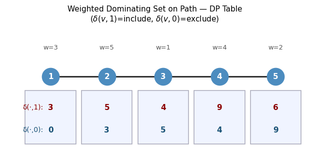The DP table \(\delta(\cdot,1)\) and \(\delta(\cdot,0)\) for a weighted path graph. Optimal solution is obtained bottom-up.

Chapter 1: Planar Graphs

Planar graphs form the gateway into structural graph theory. They are among the oldest and most thoroughly understood graph classes, and their study motivates virtually every technique encountered later in the course: embeddings, dual constructions, separator theorems, and forbidden minor characterizations all make their first appearance here. The goal of this chapter is not merely to catalog properties of planar graphs, but to understand why those properties hold and how they can be exploited algorithmically.

1.1 Definitions and Embeddings

A planar graph is one that can be drawn in the plane without edge crossings. Making this precise requires separating the drawing (an analytic object) from the combinatorial information it encodes.

To work rigorously with planarity, we need to make the notion of a “drawing” mathematically precise. The following definition captures the essential requirement: edges are continuous curves, and distinct edge interiors never meet.

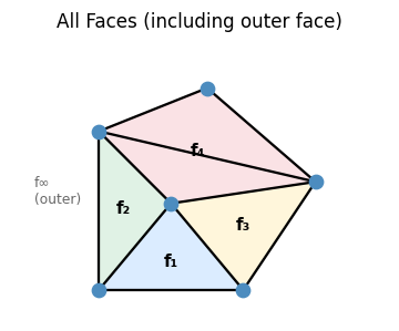
A planar drawing carves the plane into regions. These regions — the faces — are the fundamental objects of planar graph theory, and counting them correctly is what gives Euler’s formula its power.

The existence of the unique unbounded outer face is a topological fact: removing a compact graph from the plane leaves exactly one unbounded connected component.

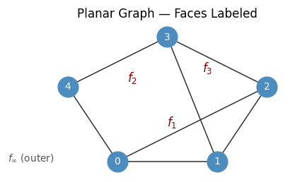A planar graph drawn without crossings. Interior faces \(f_1, f_2, f_3\) and the outer face \(f_\infty\) are labeled.

This closure under minors will become central in Chapter 6: it means that planarity is a minor-closed property, and by the Robertson–Seymour theorem this forces a finite forbidden minor characterization — which turns out to be exactly \(\{K_5, K_{3,3}\}\).

The combinatorial essence of a drawing is captured by the cyclic order of edges at each vertex. Two very different drawings can carry the same combinatorial information, so we want a discrete object that captures exactly this information.

A rotation system is a purely combinatorial object — a finite collection of cyclic orderings — with no reference to coordinates. Together with a choice of outer face, it completely encodes the planar embedding.

The combinatorial embedding is remarkably powerful: once we know the cyclic edge orders at every vertex, we can recover all faces of the drawing by following the “next edge at the far endpoint” rule, without ever consulting a geometric picture.

Every face — interior and exterior — can be identified from the rotation system alone.

The re-rooting lemma tells us that the designation of an “outer face” is a matter of convention rather than a deep structural distinction: every face of a connected plane graph can serve as the outer face. This flexibility is frequently exploited — for instance, in the dual graph construction and in the max-flow algorithm of Section 1.4.

1.2 Euler’s Formula

With the basic definitions in hand, we can now derive the most celebrated and useful theorem about planar graphs. Euler’s formula relates the three fundamental counts of a plane graph — vertices, edges, and faces — in a beautifully simple linear relation. That this relation is constant (equal to 2) for every connected plane graph is striking; it says that the topology of the drawing imposes an iron constraint on the combinatorics.

The proof strategy is characteristic of planar graph arguments: induct by reducing faces one at a time, maintaining the formula at each step. The base case — a tree, with exactly one face — is the anchor.

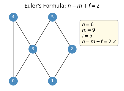Example: \(n=6\), \(m=9\), \(f=5\) gives \(6 - 9 + 5 = 2\). ✓

Euler’s formula immediately implies a tight upper bound on the number of edges in a planar graph. This edge bound is the workhorse of almost every planarity argument.

The proof uses a double-counting argument on the “face-edge incidence” — a technique that recurs throughout the course. An immediate consequence of Euler’s formula is that the number of faces is a topological invariant of the graph — any two planar drawings have the same face count.

The two bounds (\(m \leq 3n-6\) and \(m \leq 2n-4\)) immediately settle the non-planarity of the two forbidden minors.

The non-planarity of \(K_5\) and \(K_{3,3}\) is more than a curiosity: Kuratowski’s theorem asserts that every non-planar graph contains one of them as a subdivision. In this sense \(K_5\) and \(K_{3,3}\) are the complete obstruction theory for planarity.

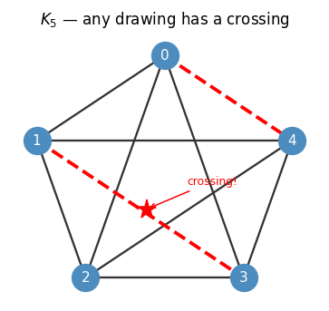\(K_5\): any planar drawing must have at least one crossing (red dashed edges). The red star marks the crossing point.

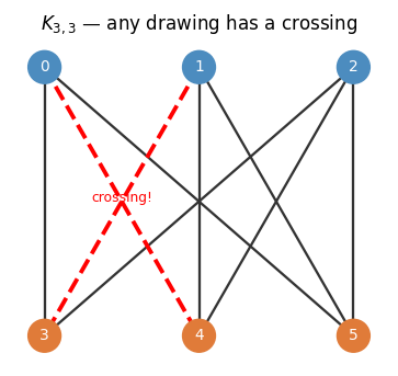\(K_{3,3}\): the complete bipartite graph on \(3+3\) vertices cannot be embedded in the plane without a crossing.

Kuratowski’s theorem is one of the great gems of combinatorics: it reduces the potentially uncountable family of non-planar graphs to just two obstructions. Wagner’s formulation replaces topological minors with graph minors, and both versions play roles in the course.

1.3 Algorithmic Consequences

The edge bound \(m \leq 3n-6\) is not only a non-planarity certificate; it is the source of several linear or near-linear-time algorithms. Every planar subgraph must satisfy the same bound, so every subgraph of a planar graph has minimum degree at most 5. This minimum-degree guarantee is the key to efficient greedy algorithms.

Minimum-degree order. Since every planar subgraph also has minimum degree \(\leq 5\) (from the edge bound), we can build a vertex order \(v_1, \ldots, v_n\) where each \(v_i\) has at most 5 predecessors in \(O(n)\) time.

Six-coloring. Greedy coloring along the minimum-degree order uses at most 6 colors. A more careful argument gives a linear-time 5-coloring algorithm.

The Four Color Theorem required a computer-assisted proof and remains one of the most computationally demanding results in mathematics. In contrast, the 5-colorability of planar graphs admits a clean inductive proof using the minimum-degree order — an instructive instance of how structural bounds yield algorithmic dividends.

Adjacency testing. Storing predecessors in the minimum-degree order allows \(O(1)\) adjacency testing using \(O(n)\) space (since each vertex has \(\leq 5\) predecessors).

Maximum clique. Using \(O(1)\) adjacency testing, we can find maximum cliques in planar graphs by checking each vertex’s constant-size predecessor set.

Dijkstra’s algorithm. Since \(m \in O(n)\) for planar graphs, binary heaps suffice and Fibonacci heaps are unnecessary: shortest paths run in \(O(n \log n)\).

1.4 Dual Graphs

One of the most powerful ideas in planar graph theory is the construction of the dual graph, which interchanges the roles of vertices and faces. Historically this duality underpins Kirchhoff’s laws for electrical networks and, in modern form, gives the clean connection between minimum cuts and shortest paths in planar graphs.

The dual is itself a plane graph (embed each dual vertex inside its corresponding face, and route dual edges across primal edges). Crucially, taking the dual twice recovers the original graph.

This involution — dualizing twice yields the original — is what makes planar duality such a clean and useful tool. It converts cut problems in the primal to cycle problems in the dual, and vice versa.

Application — polygon mesh conversion. Given a triangular mesh (a triangulated planar graph), converting it to a quadrangular mesh means finding a perfect matching in the dual graph — a classical task solvable in linear time.

Application — maximum flow via shortest paths. For an undirected flow network that is \(st\)-planar (both \(s\) and \(t\) lie on the outer face), the minimum \(st\)-cut corresponds to a shortest path in the dual. We first set up the formal definitions of flow networks.

For planar graphs, a minimum cut corresponds to a cycle in the dual. More precisely:

For st-planar graphs, this is made algorithmic via the dual network:

The key construction: add a temporary edge \(st\) on the outer face, form \(G'\), take its dual \((G')^*\), remove the dual edge between the two faces incident to \(st\), and set dual edge weights equal to primal capacities. A shortest \(s^*t^*\)-path in this network yields both the maximum flow value and a minimum cut. This result is a striking demonstration of planar duality at work: a flow problem in the primal becomes a shortest-path problem in the dual, and linear-time algorithms that would be impossible in general graphs become accessible.

1.5 NP-Hard Problems in Planar Graphs

Not everything becomes easy on planar graphs. Several fundamental problems remain NP-hard even when the input is planar, and understanding why — through carefully constructed reductions — reveals the limits of structural restrictions. The two main proof techniques exploit either the ability to simulate crossings with planar gadgets, or the fact that a simpler NP-hard problem (Planar 3-SAT) is already stated on a planar object.

Several problems remain NP-hard even restricted to planar graphs. The proof techniques are:

1. Crossing gadget: reduce from the general (non-planar) version using a gadget that simulates a crossing while preserving planarity.
2. Planarity-preserving reduction: start from an NP-hard problem already stated on planar graphs (e.g., Planar 3-SAT) and show the reduction preserves planarity.

These hardness results are important calibration points: they tell us that planarity alone is not a sufficient structural restriction for tractability. To get polynomial-time algorithms for hard problems, we need additional structural parameters — which is precisely the motivation for treewidth and the separator hierarchy developed in Chapters 3 and 4.

The crossing gadget argument works as follows. For 3-coloring, a crossing gadget is a planar subgraph on four boundary vertices \(a, a', b, b'\) such that any 3-coloring forces \(c(a) = c(a')\) and \(c(b) = c(b')\), while both same-color and different-color assignments are achievable.

Using this gadget, any graph \(G\) can be made planar while preserving 3-colorability.

Planar 3-SAT is central: given a 3-SAT formula, build a graph with one vertex per variable, one per clause, edges for (literal, clause) containment, and a cycle over variables. If this SAT graph is planar, the instance is Planar 3-SAT.

The reduction makes the SAT graph planar by rerouting the variable cycle and using crossing gadgets. The key reductions for other problems follow:

Chapter 2: Graph Drawing and Embeddings

Chapter 1 established the basic theory of planarity. This chapter turns to finer questions about how graphs are embedded: how to search a planar graph in a way that respects the embedding, how to test planarity algorithmically, and how to produce aesthetically and mathematically canonical drawings. These questions have both theoretical and practical significance — canonical orderings and straight-line drawings underlie modern graph visualization tools.

2.1 Right-First Search

Ordinary DFS ignores the geometry of a planar embedding and treats all outgoing edges symmetrically. In a plane graph, there is a canonical way to break ties: use the cyclic edge order at each vertex. Right-First Search is a DFS that breaks ties using the embedding: at each vertex, edges are explored in counter-clockwise order with the incoming edge last.

RightFirstSearch(G, v₀, e₀):
    discovered[v] = None for all v
    def recurse(v, e):
        discovered[v] = e  # arrived via e
        for eᵢ in edges at v in CCW order, with e last:
            v, w = eᵢ
            if discovered[w] is None:
                recurse(w, eᵢ)
    recurse(v₀, e₀)

The key insight is that always taking the “rightmost” option at each step produces paths with a global optimality property. To make this precise, we need to define what “rightmost” means globally.

The right-most path is the one that “hugs” the rightmost part of the plane as tightly as possible. The following lemma says that greedy right-first choices globally produce this extremal path.

This lemma is the engine behind the Menger algorithm for st-planar graphs: right-most paths in an st-planar graph are “as far apart as possible,” so finding them greedily and removing used vertices produces a maximum collection of vertex-disjoint paths.

Menger’s problem in \(st\)-planar graphs. Given an \(st\)-planar directed graph, find the maximum number of vertex-disjoint \(st\)-paths. Algorithm:

1. Temporarily insert edge \(ts\) on the outer face.
2. Run right-first search from \(s\) relative to \(ts\).
3. If \(t\) is reached, output the path, remove used vertices (excluding \(s, t\)), repeat.

Since each call only visits previously unvisited edges, total time is \(O(m + n)\). The right-most lemma guarantees optimality.

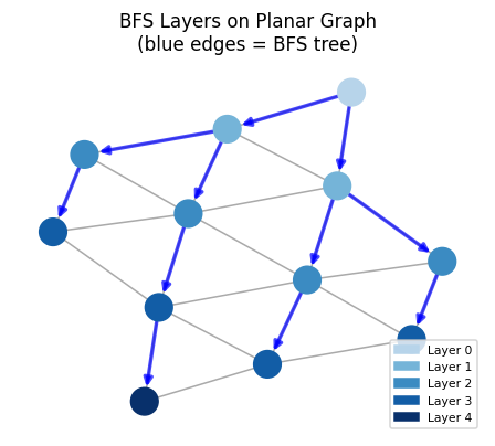BFS layering reveals structure exploitable by algorithms like Baker’s PTAS. Blue edges form the BFS tree; node shading encodes distance from the root.

2.2 Planarity Testing

A graph is planar if and only if a planar embedding exists. Recognizing planarity and constructing the embedding can both be done in linear time. This is a remarkable algorithmic achievement: planarity is a global topological property, yet it can be certified by a local, incremental DFS procedure.

The key idea is to build the embedding one DFS subtree at a time. At each step, we maintain the invariant that the partial embedding is a valid “bush form.”

The validity condition ensures that the “pending” edges (those connecting the current partial subgraph to the rest of the graph) can all be routed out through a single face, leaving room for the rest of the embedding to be appended.

The Haeupler–Tarjan algorithm runs DFS and, at each retreat from a vertex \(w\) to parent \(v\), checks whether the bush form of \(D(w)\) (descendants of \(w\)) can accommodate the edges from \(v\) into \(D(w)\) consecutively on the outer face. Two auxiliary lemmas drive the correctness argument.

This is tracked using PQ-trees — a data structure specifically designed for the problem of maintaining consecutive orderings under constraints.

PQ-trees encode a potentially exponential family of permutations in a polynomial-sized structure, and reductions are cheap precisely because the planarity constraints imposed at each DFS step are local. This amortized efficiency is what enables the linear overall runtime.

This is optimal: any algorithm must at least read the entire input graph, which takes \(\Omega(m)\) time.

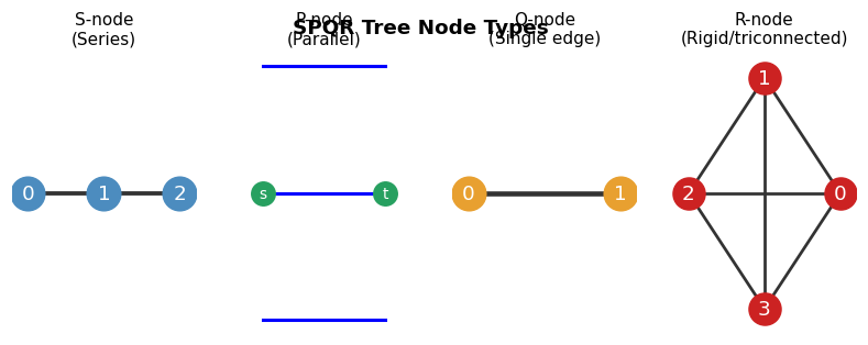The four SPQR-tree node types encode biconnected components: S (series), P (parallel), Q (single edge), R (rigid/triconnected). The SPQR tree gives a compact representation of all planar embeddings of a biconnected graph.

2.3 Triangulated Graphs and Canonical Orderings

To produce straight-line and grid drawings of planar graphs, we need a special vertex ordering that allows an inductive construction of the drawing. Triangulated graphs — those where every face is a triangle — are the natural starting point, since every planar graph can be triangulated by adding edges. The canonical ordering is the key algorithmic tool.

Triangulated planar graphs are the “densest” planar graphs possible — adding any edge would create a crossing. Three useful characterizations hold simultaneously:

The triangulated disk is the building block for inductive constructions:

The canonical ordering is designed so that each new vertex \(v_k\) “sits on top of” a consecutive arc of the current outer face, making an inductive placement of vertices geometrically consistent.

The existence of a canonical ordering is not obvious: it requires showing that there always exists a vertex whose removal leaves the graph in the right inductive state. The proof uses the structure of 2-connected triangulated disks.

Key property (maintained inductively): \(G_k = G[v_1, \ldots, v_k]\) is a triangulated disk — 2-connected, all inner faces are triangles, the outer face is a simple cycle. The predecessors of \(v_{k+1}\) form a consecutive interval on the outer face of \(G_k\).

Schnyder Wood. The canonical ordering induces a partition of the edges of a triangulated graph into 3 spanning forests (actually spanning trees, after accounting for vertex indices).

The arboricity bound is sharp: the icosahedron has arboricity exactly 3. It also implies that any planar graph can be 3-colored as a “forest” rather than a graph — a useful structural decomposition.

Straight-line embedding (Tutte / Canonical Order). The canonical ordering constructively proves that planar graphs do not need curved edges in their drawings — every planar graph has a drawing where all edges are straight line segments.

The proof strategy — place each new vertex in the interior of the triangle formed by its outer-face neighbors — is an inductive geometric argument enabled entirely by the canonical ordering.

Visibility representation. A bar visibility representation maps each vertex to a horizontal segment and each edge to a vertical segment connecting its endpoints. The canonical ordering implies every triangulated graph has a strong visibility representation, with coordinates in \([1, 3n-6] \times [1, n]\).

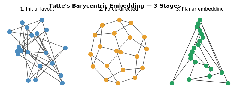Three stages of Tutte’s barycentric embedding on the dodecahedron: (1) arbitrary initial placement, (2) force-directed layout, (3) final planar embedding.

Chapter 2.5: Graph Classes Beyond Planar

Planar graphs are the starting point of structural graph theory, but they are far from the end of the story. Once we have a clean characterization of one class — planar graphs — the natural question is: what lies on either side? Are there useful sub-classes of planar graphs, and are there larger classes that capture some but not all of the planarity structure?

This chapter charts a hierarchy of graph classes organized by how “planar-like” they are. On the more restrictive side, we have outerplanar graphs (all vertices on the outer face), series-parallel graphs (built by series and parallel combinations), and Apollonian networks (built by iterating triangle subdivision). Each restriction imposes stronger structural constraints and enables more efficient algorithms. On the less restrictive side, we have near-planar graphs — those with bounded crossing number, bounded skew number, or bounded local crossing number — and 3D graphs, which can always be drawn in three dimensions without any crossings.

The deeper purpose of this survey is to calibrate our intuition for treewidth. Outerplanar graphs have treewidth at most 2; series-parallel graphs are precisely the partial 2-trees; Apollonian networks are 3-trees. Each sub-class of planar graphs sits at a specific treewidth level in the hierarchy we will make precise in Chapter 4. Understanding this hierarchy — and which problems are tractable at each level — is the conceptual scaffold for the entire second half of the course.

2.5.1 Graphs in 3D

Surprisingly, the restriction to the plane is what causes crossing problems. In three dimensions, there is so much “room” that any graph whatsoever can be drawn without crossings using only straight edges. The proof uses the moment curve — a one-dimensional algebraic variety in \(\mathbb{R}^3\) with the property that no four of its points are coplanar.

The proof places vertices on the moment curve \(\{(x, x^2, x^3) : x \in \mathbb{R}^+\}\). Any potential crossing would require 4 coplanar points on the moment curve, but Vandermonde determinants show no 3 distinct points on the moment curve are collinear, so no 4 are coplanar.

2.5.2 Near-Planar Graphs

If we must work in the plane but cannot avoid all crossings, the natural question is how few crossings are unavoidable. The crossing number of a graph is the minimum over all drawings. Allowing even one crossing dramatically expands the class — graphs of crossing number 1 include many non-planar graphs — but crossing number remains NP-hard to compute. Weaker variants (bounded skew number, bounded local crossings) give tractable recognition problems and often preserve enough planar structure for algorithmic purposes.

2.5.3 Outer-Planar Graphs

Outer-planar graphs are the simplest proper sub-class of planar graphs. The requirement that every vertex lies on the outer face is a strong restriction: it means the graph is “one-dimensional” in a sense — you can always see all vertices from the outside. This makes many hard problems tractable. For instance, any maximal outer-planar graph is a triangulated disk whose dual is a tree, so problems that require global reasoning on a general planar graph reduce to tree problems on outer-planar graphs.

The key algorithmic leverage is that outer-planar graphs have treewidth at most 2: their structure is captured by a tree of triangles (the interior dual), and the DP from Chapter 4 runs in \(O(n)\). This connection — outerplanar equals partial 2-tree — will be made precise in Section 4.4.

The vertex order from Lemma 6.2.4 admits an easy linear-time 3-coloring by greedy on this order.

2.5.4 Series-Parallel Graphs

Series-parallel graphs generalize the circuits of electrical engineering. Any resistor network built from series and parallel combinations — no Wheatstone bridge, no \(Y\)-\(\Delta\) configuration — is a series-parallel graph. The recursive construction makes many optimization problems (shortest paths with constraints, maximum flow, network reliability) solvable in linear time by a simple bottom-up computation on the SP-tree. Series-parallel graphs sit at exactly treewidth 2 in the hierarchy: they are the partial 2-trees, strictly more general than outerplanar graphs but still far more tractable than general planar graphs.

2.5.5 Apollonian Networks

Apollonian networks sit at treewidth 3 in the hierarchy. They arise naturally in geometry — the Apollonian gasket of classical circle-packing is their continuous analog — and they serve as the canonical example of 3-trees. Every Apollonian network is triangulated, planar, and has a clean recursive structure: at each step, a new vertex is inserted into a triangular face and connected to all three triangle vertices. This inductive definition gives a perfect elimination order almost by construction.

Chapter 3: Separators and Decompositions

The previous chapters developed the rich structure of planar graphs and their embeddings. We now turn to one of the most powerful consequences of planarity for algorithm design: the existence of small separators. A separator is a small set of vertices whose removal splits the graph into balanced pieces. Small separators enable divide-and-conquer algorithms with sub-quadratic running times for problems that are otherwise expensive, and they lead directly to the concept of treewidth explored in Chapter 4.

3.1 Separators

The central question is: how cheaply can we split a planar graph into balanced pieces? “Cheaply” means using few vertices as the separator. If a separator has \(s\) vertices, then to solve a problem by divide-and-conquer we pay at most \(O(s \cdot T(n/2) + s \cdot C)\) for the boundary work, where \(C\) is the per-separator-vertex cost. For the recursion to beat \(O(n^2)\), we need \(s = o(n)\). The Lipton–Tarjan theorem gives \(s = O(\sqrt{n})\), which is enough to beat quadratic time for a wide range of problems.

To measure “balance,” we allow vertices to have weights and ask that no piece of the divided graph is too heavy. This generality is important for the recursive application of the separator theorem.

A \(\frac{1}{2}\)-separator is the strongest case: every piece has at most half the total weight. Separators of size \(O(\sqrt{n})\) in planar graphs — the Lipton–Tarjan theorem — are what make the divide-and-conquer algorithms of Section 3.2 possible.

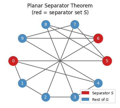The planar separator theorem guarantees a small vertex cut (red) dividing the graph into balanced parts. Here the Petersen graph is shown with a small separator highlighted.

Separators in trees. Any tree has a \(\frac{1}{2}\)-separator of size 1: pick the root \(r\), walk to the heaviest child repeatedly until no child’s subtree exceeds \(\frac{1}{2} w(V)\). The current vertex is the separator.

The proof strategy is elegant: the onion peeling structure of planar graphs (Section 6.1) allows us to sparsify the graph to something of bounded treewidth, on which small separators are guaranteed. The optimal \(k = \Theta(\sqrt{n})\) balances the two separator contributions.

3.2 Divide-and-Conquer with Separators

The Planar Separator Theorem is not just a structural curiosity — it is a powerful algorithmic tool. For problems whose running time scales superlinearly with the number of vertices, a balanced separator lets us split the work, solve independently, and combine. The recursion tree has depth \(O(\log n)\) and at each level, the separator vertices require special attention.

Planar separators enable divide-and-conquer algorithms with sub-quadratic running times:

Shortest directed cycle. Use the \(\frac{1}{2}\)-separator recursively. At each level, run Dijkstra from each separator vertex. Recursion: \(T(n) = \sum T(n_i) + O(\sqrt{n} \cdot n \log n)\), yielding \(T(n) \in O(n^{3/2} \log n)\).

Global minimum cut. By duality, a minimum cut in an undirected planar graph corresponds to a shortest cycle in the dual. The same divide-and-conquer approach applies.

Maximum matching. Build the matching recursively in each flap, then augment along paths passing through each separator vertex. Total time: \(O(n^{3/2} \log n)\).

3.3 Separator Hierarchies and Pathwidth

We have used separators as a computational device. Now we show that the recursive separator structure carries deep information about the graph’s intrinsic complexity: it gives an explicit upper bound on pathwidth, and through pathwidth, on treewidth. This is the bridge that takes us from the “divide-and-conquer” world of separator algorithms into the “bag decomposition” world of treewidth.

The recursive application of the separator theorem produces a hierarchical decomposition of the graph that is more than just a computational convenience — it encodes the graph’s structure in a form that directly gives bounds on pathwidth and treewidth. This connection is the bridge between the separator world and the decomposition world of Chapter 4.

The hierarchy records the full recursive structure: at each level, the separator vertices are the “interface” between the two halves. Collecting these interfaces along a root-to-leaf path gives a sequence of bags that forms a path decomposition.

From a hierarchy, one extracts a path decomposition by letting each leaf’s bag be the union of all ancestor separators. This yields:

The tightness of the \(k \times k\)-grid example shows that the separator theorem is essentially sharp for planar graphs: neither the separator size nor the treewidth bound can be improved to \(o(\sqrt{n})\) in general. This motivates the quest for subclasses with smaller treewidth, addressed in the next chapter.

Chapter 4: Tree Decompositions and Treewidth

This is the heart of the course. Tree decompositions generalize interval graph representations and allow dynamic programming to be lifted from trees to any graph with small “tree-like” structure. The concept of treewidth — the minimum width of any tree decomposition — emerges as the master parameter of the whole theory: small treewidth enables efficient algorithms for virtually all natural graph problems, while large treewidth (specifically, containing a large grid minor) signals computational hardness.

4.1 Interval Graphs and Chordal Graphs

Before defining tree decompositions in full generality, it is instructive to study two families where the decomposition structure is already visible: interval graphs and chordal graphs. These classes admit polynomial-time algorithms for problems that are NP-hard in general, and understanding why sets up the machinery for bounded-treewidth graphs.

Here is a useful mental model. Think of Gaussian elimination on a sparse symmetric matrix: when you eliminate a variable, you fill in edges between its remaining neighbors. If those neighbors already form a clique, no new edges are created — the matrix stays sparse. A graph where every vertex can be eliminated in this “fill-free” order is precisely a chordal graph, and the elimination order is its perfect elimination order. This connection is not merely analogical: Gaussian elimination on the adjacency matrix of a chordal graph runs without any fill-in, which is why chordal graphs are the key to efficient sparse linear solvers. The algorithm we study — Maximum Cardinality Search — is essentially the graph-theoretic version of choosing the best pivot at each elimination step.

Interval graphs model scheduling conflicts, molecular sequence overlaps, and a host of other practical problems where “overlap” is the fundamental relation. Their structure is essentially one-dimensional, which is why they are so tractable.

Chordality is the abstract algebraic generalization of interval graph structure: a graph is chordal when it has no “long” induced cycles, i.e., when every cycle can be “shortcut” by a chord.

Every interval graph is chordal. Every tree is chordal.

The key algorithmic handle on chordal graphs is the perfect elimination order (PEO): an ordering in which each vertex, together with its earlier neighbors, forms a clique. The PEO is the sequence in which vertices can be “safely eliminated” — removed from the graph without disturbing the clique structure of their neighborhood. Think of building up the graph in reverse: each new vertex \(v_i\) arrives and finds that all of its already-placed neighbors are mutually adjacent, forming a clique. This is exactly the condition that makes greedy coloring optimal and that allows the tree decomposition to be read off from the order.

The PEO is precisely the order in which vertices can be eliminated — removed without destroying the clique structure of their neighborhood. This turns out to characterize chordality exactly.

This equivalence is the key to understanding chordal graphs algorithmically: we can recognize them, solve optimization problems on them, and build their tree decompositions, all via the PEO.

Maximum Cardinality Search (MCS). Repeatedly pick the vertex with the most already-chosen neighbors (breaking ties arbitrarily). This runs in \(O(m + n)\) and produces a PEO of any chordal graph.

The PQ-tree reappears here: the consecutive ordering of cliques in an interval graph is precisely the kind of constraint that PQ-trees were designed to encode and check efficiently.

Polynomial algorithms in chordal graphs. The PEO does for chordal graphs what the minimum-degree ordering did for planar graphs: it provides a vertex ordering that makes greedy algorithms optimal. Because each vertex’s predecessor set is a clique, there is no “wasted” coloring and no “hidden” interference that greedy might miss.

Using a PEO:

• Coloring: Greedy on the PEO gives the optimal \(\chi(G) = \omega(G)\) coloring.
• Maximum independent set: Greedy in reverse PEO (the marked-set argument) gives an optimal solution.
• Maximum clique: \(\omega(G) = \max_i(\text{indeg}(v_i) + 1)\).

Note: Dominating Set is NP-hard in chordal graphs (reduce from Vertex Cover in general graphs by subdividing every edge and adding all clique edges between original vertices). This shows that even well-structured graph classes can retain NP-hard problems — treewidth, not chordality, is the right parameter for universal tractability.

4.2 Strong Tree Decompositions

The connection between interval graphs and path decompositions, and between chordal graphs and tree decompositions, can be made precise via strong decompositions.

Let us pause to consolidate what the perfect elimination order tells us. For a chordal graph, the set \(\{v_i\} \cup \text{pred}(v_i)\) — vertex \(v_i\) together with its earlier neighbors — is a clique, and these cliques can be organized into a tree structure where adjacent bags share a large overlap. This is the strong tree decomposition: the tree whose nodes are the maximal cliques and whose edges connect cliques that differ by exactly one vertex. The “strong” refers to the biconditional in condition (iii): every pair sharing a bag is adjacent, and conversely. This is only possible for chordal graphs. For general graphs, we must relax this to the weak tree decomposition — every edge is covered by a bag, but two vertices sharing a bag need not be adjacent. That relaxation is the key to making the theory work for arbitrary graphs.

The perfect elimination order of a chordal graph encodes a tree-like structure: each vertex’s predecessor set is a clique, and these cliques can be organized into a tree. This is the strong tree decomposition — a tree whose bags are the maximal cliques, with edges representing shared elements. It is the prototype for the more general tree decomposition.

Condition (iii) is the “if and only if” form: every edge is represented in some bag, and every pair of vertices sharing a bag is adjacent. This biconditional makes the decomposition exact — the tree completely encodes the graph structure.

The proof is constructive in both directions: given a chordal graph we build its strong tree decomposition via the PEO, and given any strong tree decomposition we recover a PEO by traversal. The two structures are in perfect correspondence.

4.3 Tree Decomposition and Treewidth

The strong tree decomposition requires the “if and only if” edge condition — every pair sharing a bag must be adjacent. For general (non-chordal) graphs, this is impossible. The solution is to relax to the weak tree decomposition, which only requires that edges are covered by bags, not that all pairs sharing a bag are adjacent. This relaxation is what allows tree decompositions to capture graphs far beyond the chordal class.

Before the definition, let us build intuition for what a tree decomposition is. Picture the graph \(G\) spread out on a table. A tree decomposition finds a way to “cover” \(G\) with overlapping clusters — the bags — arranged in a tree. Each vertex of \(G\) appears in one or more bags, and the bags containing any fixed vertex form a connected subtree (the connectivity condition). Every edge of \(G\) is “witnessed” by at least one bag that contains both its endpoints.

The tree structure means that if you take any bag \(X_i\) and remove it, the host tree splits into subtrees, and the corresponding subgraphs of \(G\) on each side can only interact through \(X_i\) itself. This is the fundamental separation property: \(X_i\) is a separator between the two sides. The width of a decomposition is one less than the size of the largest bag; we subtract one so that trees themselves (which have bags of size 2, one vertex per edge) get treewidth 1. Treewidth 0 means the graph is a collection of isolated vertices; treewidth 1 means a forest; treewidth 2 means outerplanar or series-parallel; treewidth \(k\) means “as complex as a \(k\)-tree but no more.”

The treewidth of a graph is the minimum width over all possible tree decompositions. Finding the optimal decomposition is NP-hard in general — but the parameter itself, once computed or approximated, unlocks efficient algorithms for an enormous range of problems.

The weaker condition means that a tree decomposition is not unique — every graph admits many tree decompositions of varying widths. We seek the decomposition of minimum width.

The shift to \(|X_i| - 1\) (rather than \(|X_i|\)) is a normalization convention that makes trees have treewidth 1 (every bag has size 2 = 1 + 1) and cliques have treewidth \(n-1\). Treewidth measures “how far from a tree the graph is,” with trees at one extreme and dense graphs at the other.

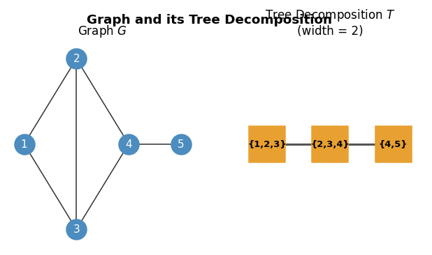A graph \(G\) and a tree decomposition of width 2. Each bag covers a clique in the supergraph.

The following theorem collects the most important equivalent characterizations of bounded treewidth, connecting the decomposition definition to a concrete graph-theoretic construction.

This equivalence is the foundation of efficient DP on bounded-treewidth graphs: characterization 1 gives a concrete inductive construction, characterization 2 connects to the PEO theory of Section 4.1, and characterization 3 is the algorithmic handle.

Property (b) — that treewidth is minor-monotone — is why treewidth fits so naturally into the Robertson–Seymour theory of Chapter 6. Property (d) calibrates our intuition: the \(k \times k\)-grid is the “most tree-unlike” planar graph of its size, and treewidth exactly captures this.

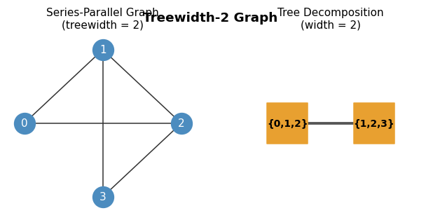A series-parallel (treewidth-2) graph and its width-2 tree decomposition. Bags of size 3 correspond to the clique-number \(\omega = 3 = k+1\).

4.4 k-Trees and Partial k-Trees

Treewidth is defined as a minimum over all possible tree decompositions — an existential definition that does not immediately suggest what graphs of treewidth exactly \(k\) look like. The \(k\)-tree provides the answer: it is the canonical graph of treewidth \(k\), obtained by the simplest possible inductive construction, and every graph of treewidth \(\leq k\) is a subgraph (partial \(k\)-tree) of one.

To make the concept of bounded treewidth concrete, it helps to have an explicit recursive construction. A \(k\)-tree is built by starting with a \(k\)-clique and repeatedly adding vertices, each connected to an existing \(k\)-clique. This is the simplest graph of treewidth exactly \(k\).

A \(k\)-tree is the “maximally dense” graph of treewidth \(k\): we cannot add any vertex without either raising treewidth above \(k\) or creating a duplicate. A partial \(k\)-tree is simply any subgraph of a \(k\)-tree — equivalently, any graph of treewidth at most \(k\). The partial 1-trees are forests. The partial 2-trees are exactly the series-parallel graphs. The partial 3-trees include all planar graphs of treewidth 3, and the Apollonian networks (defined in Chapter 2.5) are exactly the 3-trees. This concrete characterization via the inductive construction is what makes it easy to build tree decompositions explicitly: the PEO of the host \(k\)-tree provides the decomposition for any partial \(k\)-tree subgraph.

The inductive construction is transparent: each new vertex is connected to exactly \(k\) existing vertices forming a clique, so the structure grows “uniformly” in a tree-like fashion.

The \(k\)-trees are exactly the chordal graphs with \(\omega = k+1\) and the exact edge count \(m = kn - \binom{k}{2} - \frac{k}{2}\). Partial \(k\)-trees (spanning subgraphs of \(k\)-trees) are exactly the graphs of treewidth \(\leq k\).

Planar instances:

• Trees = partial 1-trees.
• Maximal outer-planar graphs = 2-trees; outer-planar graphs = partial 2-trees = SP-graphs.
• Apollonian networks = 3-trees; partial 3-trees include all planar graphs of low treewidth.

4.5 Series-Parallel Graphs

Series-parallel graphs are a particularly clean family of graphs with treewidth at most 2. They are defined by a recursive construction that mimics the series and parallel combinations of electrical circuits — a connection that is more than coincidental, since SP-graphs are exactly the graphs for which Kirchhoff’s equations can be solved by simple elimination.

The recursive structure is captured by the SP-tree, which makes many algorithms on SP-graphs straightforward bottom-up computations.

The SP-tree is a binary tree encoding the construction. SP-graphs are exactly the partial 2-trees. Recognition runs in linear time by repeatedly contracting degree-2 vertices or removing parallel edges.

The proof is constructive: the SP-tree directly encodes a tree decomposition. This is a paradigm that recurs in more general settings — an explicit recursive construction of the graph gives an explicit tree decomposition.

4.6 Branchwidth and Pathwidth

Having established treewidth as the central parameter, it is natural to ask whether it is the right parameter for every application. The answer is nuanced. For most theoretical purposes — FPT algorithms, Courcelle’s theorem, the Robertson–Seymour theory — treewidth is ideal. But for specific algorithmic tasks, particularly on planar graphs, two variants offer advantages: branchwidth (computable in polynomial time for planar graphs) and pathwidth (relevant for linear-arrangement problems and graph searching games).

Treewidth is not the only width parameter that captures tree-like structure. Two important variants — branchwidth and pathwidth — offer different trade-offs and are useful in different algorithmic contexts.

Think of the three parameters as measuring “tree-likeness” in different ways. Treewidth puts vertices in the bags and asks that the host tree have a connected subtree for each vertex. Branchwidth puts edges at the leaves of a binary tree and measures how many vertices are “shared” when you cut any arc. Pathwidth is the most restrictive: the host tree must be a path, meaning the bags are arranged in a linear sequence. A graph can have small treewidth but large pathwidth if its tree structure fans out in many directions — for instance, a balanced binary tree has treewidth 1 (it is a tree!) but pathwidth \(\Theta(\log n)\).

The three parameters are related by inequalities: \(\text{tw}(G) \leq \text{pw}(G)\) always, and \(\text{bw}(G)\) is within a factor of \(3/2\) of \(\text{tw}(G)\). But their computational complexity differs sharply. All three are NP-hard to compute exactly on general graphs. However, branchwidth of planar graphs can be computed exactly in \(O(n^2)\) time via the sphere-cut decomposition — a remarkable exception that makes branchwidth the preferred parameter for exact planar graph algorithms.

Pathwidth has an elegant alternative characterization as the vertex-separation number — the number of vertices one must “remember” when processing the graph left to right in the best linear arrangement. This connects pathwidth to graph searching (the “cop number” for node searching) and to register allocation in compilers, where the pathwidth of a program’s dependency graph bounds the number of registers needed.

The branch decomposition is defined in two equivalent ways:

Branchwidth and treewidth measure essentially the same thing, as confirmed by the following quantitative relationship.

The two parameters are within a constant factor of each other, so for most purposes they are interchangeable. However, branchwidth has a decisive computational advantage for planar graphs: it can be computed exactly in polynomial time.

Branchwidth of planar graphs is computable in \(O(n^2)\) time (and the optimal branch decomposition is sphere-cut). This gives a \(\frac{3}{2}\)-approximation for treewidth of planar graphs.

Pathwidth is a stronger condition than treewidth: \(\text{tw}(G) \leq \text{pw}(G)\) always, and the gap can be logarithmic. But for linear-time algorithms and certain graph searching problems, pathwidth is the natural parameter.

The following linear-arrangement definitions are the key to proving the pathwidth equivalences.

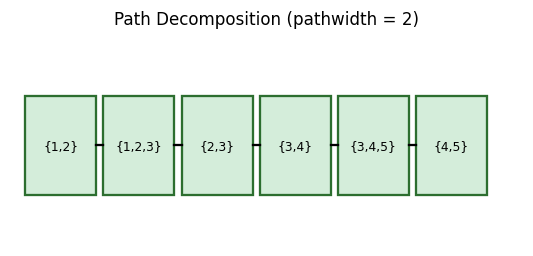A path decomposition: bags are arranged linearly, each consecutive pair differs by at most one vertex (in a “nice” decomposition).

The equivalence between pathwidth and interval graph containment mirrors the equivalence between treewidth and chordal graph containment. In both cases, the “forbidden subgraph” perspective and the “decomposition” perspective give the same parameter.

Pathwidth of trees. Any tree has pathwidth at most \(\log_2 n\). A tree is a \(k\)-caterpillar iff its pathwidth is exactly \(k\); this gives a recursive characterization computable in linear time.

Computing width parameters is NP-hard: treewidth, pathwidth, and cutwidth are all NP-hard to compute exactly, even in restricted graph families. However, computing branchwidth of planar graphs is polynomial. This computational gap between exact treewidth computation (NP-hard) and the FPT algorithms that use treewidth as a parameter motivates the approximation algorithm discussed in Section 6.2.

Chapter 5: Fixed-Parameter Tractability

Treewidth was introduced in Chapter 4 as a structural parameter measuring the “tree-likeness” of a graph. This chapter cashes in on that investment: graphs of small treewidth admit efficient dynamic programming algorithms for a wide range of hard combinatorial problems. The key insight is that a tree decomposition breaks a problem into subproblems that interact only through small “interfaces” — the bags — and DP over the decomposition solves the original problem in time exponential only in the treewidth, not in \(n\).

5.1 Dynamic Programming in Partial \(k\)-Trees

Why does bounded treewidth enable efficient dynamic programming? The answer lies in the separation property of tree decompositions. Consider any node \(i\) in the decomposition tree and remove its bag \(X_i\). The tree splits into subtrees, and the corresponding subgraphs of \(G\) can only “communicate” through \(X_i\): no edge crosses from one side to the other without touching \(X_i\). This is exactly the condition needed to apply the DP principle — once you fix the “state” of the vertices in \(X_i\), the two halves become independent subproblems. With \(|X_i| \leq k+1\), the number of states is at most \(2^{k+1}\) (for problems where the state is a subset of the bag), so the total work per node is exponential in \(k\) but only polynomial in \(n\).

To make this concrete: when we solve maximum weight independent set by DP on a tree decomposition, the state at each bag \(X_i\) is the intersection of the independent set with \(X_i\) — just a subset of \(k+1\) vertices. The DP table has \(O(2^k)\) entries per node, and there are \(O(n)\) nodes, giving an \(O(2^k n)\) algorithm. This is fixed-parameter tractable: polynomial in \(n\) for any fixed \(k\), with only the exponential dependence on \(k\) paying the price of generality.

Dynamic programming on trees exploits the fact that subtrees interact only through their root. Tree decompositions generalize this: the bag at a join node is the “interface” between two subproblems. The DP state records all information about the solved subgraph that is relevant to the remaining decisions — precisely the contents of the current bag.

Here is the fundamental template that underlies all DP algorithms on tree decompositions. Root the decomposition tree. For each node \(i\) (processed bottom-up), and for each possible “state” of the vertices in the current bag \(X_i\), compute the best solution for the subgraph \(G[Y_i]\) (all vertices in bags at or below \(i\)) that is consistent with that state. The key insight is that the state only needs to describe what is in the current bag — not the entire history of how we got here. The bag acts as a firewall: once you know the state of \(X_i\), the two sides of the decomposition are independent.

For maximum weight independent set, the state of bag \(X_i\) is simply a subset \(Z \subseteq X_i\) — the intersection of the independent set \(I\) with the current bag. There are at most \(2^{k+1}\) such subsets if the bag has size \(k+1\). The DP transitions are:

• At a leaf node: check directly whether \(Z\) is an independent set.
• At an introduce node (adding vertex \(x\)): if \(x \in Z\), verify no neighbor of \(x\) in the bag is also in \(Z\), and add \(w(x)\) to the child value.
• At a forget node (removing vertex \(x\)): take the maximum over states \(Z \cup \{x\}\) and \(Z \setminus \{x\}\) from the child.
• At a join node (merging two independent subtrees): add the values from the two children and subtract \(w(Z)\) to avoid double-counting the bag vertices.

This same template — with different state definitions — applies to weighted dominating set, maximum matching, graph coloring, and any other property expressible in terms of local constraints on the vertices in each bag. The exponential factor \(2^k\) in the runtime reflects the number of bag states; the linear factor in \(n\) reflects the size of the decomposition tree.

DP on trees — maximum weight independent set. Define \(\alpha(v, 1)\) (best IS weight in \(T_v\) including \(v\)) and \(\alpha(v, 0)\) (excluding \(v\)):

Nice Tree Decomposition. Every partial \(k\)-tree has a tree decomposition in which each node is one of four types:

• Leaf node: no children, single vertex.
• Introduce node: one child; \(X_i = X_j \cup \{x\}\).
• Forget node: one child; \(X_i = X_j \setminus \{x\}\).
• Join node: two children; \(X_i = X_{j_1} = X_{j_2}\).

This result is fundamental: it shows that the exponential dependence on \(k\) is the price of generality, while the polynomial dependence on \(n\) means the algorithm is efficient when \(k\) is small. For planar graphs, \(k = O(\sqrt{n})\) from the separator theorem, giving sub-exponential overall runtime.

5.2 Fixed-Parameter Tractability

The DP algorithm for independent set on partial \(k\)-trees is an instance of a broader paradigm: fixed-parameter tractability, where the “hard” part of the computation depends only on a structural parameter \(k\), not on the input size \(n\).

FPT is the appropriate notion of tractability when the parameter \(k\) is small in practice even if the input is large. Parameterized complexity theory (the study of what is and is not FPT) is a rich field; here we focus on treewidth as the parameter.

Independent set on partial \(k\)-trees is FPT parameterized by treewidth. The key observation: for any problem that can be solved by the bag-DP scheme, the number of states per node is at most \(2^{k+1}\), and there are \(O(n)\) nodes.

5.3 Monadic Second-Order Logic and Courcelle’s Theorem

Every specific DP algorithm on tree decompositions — independent set, dominating set, Hamiltonian cycle, matching — follows the same template: define a state space, write down transitions, read off the answer. Courcelle’s theorem asks: is there a single algorithm that handles all such problems automatically? The answer is yes, provided we can express the problem in the right logical language.

The language is Monadic Second-Order Logic (MSOL): first-order logic augmented with variables ranging over sets of vertices (or edges), and set membership as a predicate. MSOL is expressive enough to capture connectivity, colorability, Hamiltonicity, and most natural graph properties — yet it is restricted enough that model checking on bounded-treewidth graphs is efficient. The key insight is that the DP automaton for any MSOL formula can be computed from the formula itself, and its state space depends only on the formula and the treewidth, not on the input graph.

Rather than designing bespoke DP algorithms for each problem, Courcelle’s theorem provides a meta-theorem: any property expressible in a suitable logic is automatically FPT in treewidth. This is one of the most powerful and elegant results in algorithmic graph theory.

MSOL allows quantification over vertices and vertex sets, membership tests, boolean operations, adjacency predicates \(\text{adj}(u, v)\), and monadic quantifiers. MSOL2 additionally allows edge sets and edge-incidence predicates.

Expressible properties: graph connectivity, bipartiteness, \(k\)-colorability, Hamiltonicity (MSOL2), perfect matching (MSOL2), dominating set, independent set, and many more.

Courcelle’s theorem is one of the most powerful meta-theorems in algorithmic graph theory: instead of designing bespoke DP algorithms, one can merely formalize the problem in MSOL2 and apply the theorem. The price paid is a function \(f(k)\) that can be enormous — towers of exponentials in \(k\) — but for small constant \(k\), the linear-in-\(n\) runtime is practically useful.

Chapter 6: Graph Minors

The final chapter brings together the structural and algorithmic perspectives developed throughout the course.

We have now built a complete toolkit: planar graphs and their embeddings (Chapters 1–2), separators and treewidth (Chapters 3–4), and FPT algorithms on bounded-treewidth graphs (Chapter 5). The question now becomes: how do we bring these tools to bear on graphs that are not already of bounded treewidth? And what is the ultimate organizing principle that explains why planar graphs, bounded-genus graphs, and bounded-treewidth graphs all admit good algorithms?

The answer is graph minors. A graph \(H\) is a minor of \(G\) if \(H\) can be obtained from \(G\) by deleting vertices, deleting edges, and contracting edges. Minor containment is a powerful and natural quasi-order on graphs: it respects all the structural properties we care about (planarity, treewidth, genus are all minor-monotone), and it has the remarkable property — the Robertson–Seymour theorem — of being a well-quasi-order on all finite graphs.

This chapter develops three major results. First, Baker’s scheme: an approximation framework for planar graphs that uses the onion-peeling structure to reduce to bounded-treewidth subproblems. Second, the Grid Minor Theorem: a fundamental dichotomy asserting that every graph either has small treewidth or contains a large grid as a minor. Third, the Robertson–Seymour Graph Minor Theorem: every minor-closed class has finitely many forbidden minors, giving polynomial-time recognition algorithms for any such class. Graph minors provide the “right” notion of substructure for planar and bounded-treewidth graphs: a graph \(H\) is a minor of \(G\) if \(H\) can be obtained by deleting and contracting edges. The Robertson–Seymour Graph Minor Theorem — proved over two decades in twenty papers — is the culmination: every minor-closed class of graphs has a finite forbidden minor characterization, leading to polynomial-time recognition algorithms for any minor-closed class.

6.1 \(k\)-Outer-Planar Graphs and Baker’s Scheme

Before reaching the full power of the Robertson–Seymour theory, we develop Baker’s PTAS for planar graph optimization. The key structural fact is that planar graphs have a hierarchical “onion” structure — successive outer-face deletions — and graphs that are deep in this hierarchy have small treewidth, enabling exact DP.

Baker’s scheme (1994) is one of the most elegant ideas in approximation algorithms. The central observation is that a planar graph can be “peeled” like an onion: remove the outer face to get a smaller planar graph, repeat. The \(i\)-th layer \(L_i\) consists of the vertices on the outer face after \(i-1\) peelings. A graph with only \(k\) layers is \(k\)-outer-planar and has treewidth at most \(3k\) — giving an exact DP solution in time exponential in \(k\) but linear in \(n\).

The PTAS idea is then disarmingly simple: for a \((1-\epsilon)\)-approximation, choose \(k = \lceil 1/\epsilon \rceil\). Partition the layers into \(k\) groups — layers \(\{1, k+1, 2k+1, \ldots\}\), layers \(\{2, k+2, 2k+2, \ldots\}\), and so on. For each group \(i\), remove the layers in group \(i\) from the graph; the remainder is \(k\)-outer-planar (the layers “close up” after removal) and solvable exactly by DP. By an averaging argument, at least one of the \(k\) choices loses at most a \(1/k \leq \epsilon\) fraction of the optimal solution weight. Return the best of the \(k\) solutions. The total runtime is \(O(k \cdot 2^{3k} \cdot n)\) — polynomial in \(n\) for fixed \(\epsilon\), and as \(\epsilon \to 0\) the exponent grows, giving the classic PTAS tradeoff.

The \(k\)-outer-planar graphs are the planar graphs of “bounded depth” in the onion peeling order. Their bounded treewidth follows from the onion structure. Some combinatorial properties:

This treewidth bound is the engine of Baker’s PTAS: by discarding one onion layer in eleven, we make the remainder \(k\)-outer-planar and thus tractable by DP.

Baker’s scheme is elegant in its simplicity: try all \(k+1\) possible “layers to remove,” solve the remaining bounded-treewidth problem exactly, and take the best result. The averaging argument guarantees that at least one attempt loses at most an \(\epsilon\) fraction of the optimum.

The approximation generalizes to any problem polynomial on bounded-treewidth graphs for any graph class with locally bounded treewidth (bounded genus graphs, 1-planar graphs, etc.).

6.2 Approximating Treewidth

Computing treewidth exactly is NP-hard even for very restricted graph families. This creates a practical dilemma: the FPT algorithms of Chapter 5 need a tree decomposition as input, but producing one is itself hard. The resolution is approximation. For algorithmic purposes, a decomposition of width at most \(4k + 4\) is nearly as useful as one of width \(k\): the DP tables grow by at most a constant exponent. The following algorithm achieves a 4-approximation and is itself FPT in \(k\), making the overall pipeline FPT even when the decomposition must be computed from scratch.

But for many applications, an approximate tree decomposition suffices — as long as its width is within a constant factor of optimal. The following result gives a practical FPT algorithm that either certifies small treewidth or reports that treewidth is large.

The key subroutine: for a set \(W \subseteq V\), finding the minimum \(W\)-separation of balance \(\frac{2}{3}\) reduces to minimum vertex cuts between auxiliary sources (Menger’s theorem), with \(2^{|W|}\) bipartitions to try. This expands to a full tree decomposition by a recursive application that is FPT in \(k\).

6.3 Grid Minors

The Grid Minor Theorem is the deepest structural result in the course. It establishes a fundamental dichotomy: a graph either has small treewidth (and is thus algorithmically tractable) or contains a large grid as a minor (witnessing that it is “essentially planar at large scale” and thus as hard as the hardest planar instances). This dichotomy is the cornerstone of the Robertson–Seymour theory.

Why is the grid the right “universal” large-treewidth graph? The \(k \times k\)-grid has treewidth exactly \(k\) — this is Lemma 10.3.6, and it is tight. If we try to separate the grid into two pieces of size \(\leq n/2\), we must cut at least \(k\) vertices (one per row or column). The grid is thus the canonical hard case for treewidth: dense, symmetric, with no shortcuts.

The Grid Minor Theorem turns this observation into a characterization: large treewidth is the only obstruction to structural simplicity. More precisely, if \(\text{tw}(G) \geq f(k)\), then \(G\) must contain a \(k \times k\)-grid as a minor. The function \(f(k)\) has been substantially improved over the decades: Robertson and Seymour’s original bound was super-exponential, but Chekuri and Chuzhoy (2016) showed \(f(k) = k^{O(1)}\) (polynomial). For planar graphs, the theorem is cleaner: either \(G\) contains a \(k \times k\)-grid minor, or \(\text{tw}(G) \leq 5k - 5\). This linear bound is the engine behind bidimensionality theory — a broad framework for designing FPT algorithms on planar graphs by showing that the solution size on a \(k \times k\)-grid grows as \(\Theta(k^2)\), so bounded solution size forces bounded treewidth and thus efficient DP.

The Grid Minor Theorem gives the converse to the trivial observation that the \(k \times k\)-grid has treewidth \(k\): large treewidth forces the presence of a large grid minor.

For planar graphs, this dichotomy is particularly clean:

The proof uses right-first search to find \(k\) vertex-disjoint \(v_N v_S\)-paths and \(k\) vertex-disjoint \(v_E v_W\)-paths; intersecting them gives the grid minor. The planarity of the graph is essential: in a non-planar graph, finding disjoint crossing paths is much harder.

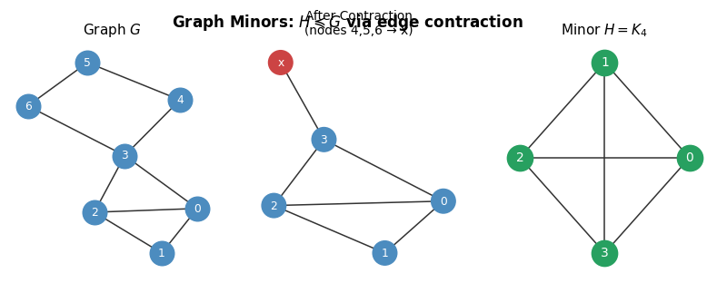\(K_4\) arises as a minor of the larger graph \(G\) by contracting vertices 4, 5, 6 into a single vertex \(x\).

6.4 Testing Minor Membership

The Grid Minor Theorem has a striking algorithmic consequence: testing whether a fixed graph \(H\) is a minor of an input graph \(G\) is polynomial for any fixed \(H\). The argument is two-step. First, check whether \(\text{tw}(G) \leq f(|H|)\): if not, by the Grid Minor Theorem \(G\) contains a large grid minor, from which one can extract any fixed pattern. If yes, the treewidth is bounded by a constant depending only on \(H\), and Courcelle’s theorem gives a linear-time algorithm. This yields a polynomial runtime for each fixed \(H\) — a remarkable unification of the structural and logical approaches.

The Grid Minor Theorem and Courcelle’s theorem combine to give a general minor testing algorithm: express the minor embedding in MSOL2 and apply the treewidth-based FPT algorithm. For planar minors, an even cleaner result is available.

This result says that, for graphs of bounded treewidth, minor testing is linear in \(n\) for any fixed \(H\). The exponential dependence on \(|H|\) is unavoidable in general, but for small patterns it is not an obstacle.

For planar \(H\) and general \(G\):

The planarity of the pattern \(H\) is what makes this possible: planar patterns have “local” embedding conditions that can be checked efficiently.

6.5 The Graph Minor Theorem

We arrive at the crown jewel of the entire course, and one of the deepest theorems in twentieth-century combinatorics: the Robertson–Seymour Graph Minor Theorem. To appreciate its power, recall the structure of the course. We have seen that planar graphs are characterized by two forbidden minors (\(K_5\) and \(K_{3,3}\)). We have seen that forests are characterized by one forbidden minor (\(K_3 = C_3\)). And we have seen that graphs of treewidth at most 2 are characterized by one forbidden minor (\(K_4\)). In each case, a minor-closed class is described by finitely many “obstructions.” Is this always the case?

The naive answer might be “no” — after all, chordal graphs require forbidding infinitely many induced subgraphs (\(C_4, C_5, C_6, \ldots\)). But the key is the choice of relation. The Robertson–Seymour theorem asserts that for the minor relation, the answer is always yes: every minor-closed class is described by finitely many forbidden minors, no matter how complex the class. The proof required twenty papers and over two decades of work; it is widely regarded as the deepest theorem in graph theory.

The logical heart of the theorem is well-quasi-ordering (WQO). A partial order is WQO if every infinite sequence contains an increasing pair — equivalently, there are no infinite antichains. The Robertson–Seymour theorem asserts that the minor order on all finite graphs is WQO. This is not obvious: the minor relation is defined by a complex sequence of operations (deletion, contraction), and graphs can be arbitrarily complicated. The proof proceeds inductively through graph classes ordered by treewidth, using Kruskal’s WQO theorem for trees as the base case and the Grid Minor Theorem to handle graphs of large treewidth.

The algorithmic consequence is striking: once we know that every minor-closed class has a finite forbidden minor set, and once we know (from Section 6.4) that testing for any fixed minor is polynomial, we get a polynomial-time recognition algorithm for every minor-closed class — even classes whose forbidden minors we cannot explicitly compute. The existence of the algorithm is guaranteed by the theorem; we need not know the forbidden minors. This is a rare and beautiful example of a non-constructive existence proof having a direct algorithmic consequence.

Minor-closed classes are classes closed under taking minors (edge deletion, vertex deletion, edge contraction). Examples: forests, planar graphs, graphs of bounded genus, graphs of bounded treewidth.

The WQO property is what we want for graphs: if the minor order is a WQO, then every downward-closed set (minor-closed class) is determined by a finite set of minimal excluded elements — the forbidden minors. The formal development proceeds through several lemmas.

The proof builds up WQO classes inductively. Key stepping stones:

The proof is a tour de force of structural graph theory, weaving together all the major themes of the course: treewidth, planar separators, grid minors, and genus. The twenty-paper series that established this result took Robertson and Seymour over two decades to complete.

What makes the Robertson–Seymour theorem so philosophically satisfying is that it closes the loop on the entire course. We started with planar graphs and their two forbidden minors. We developed treewidth as the central parameter. We proved that large treewidth forces a large grid minor. We established FPT algorithms via tree decompositions. And now we learn that all of this structure — the entire ladder of graph classes — is governed by a single organizing principle: the finiteness of forbidden minors in the minor order. Every graph class that is closed under taking minors, no matter how it was defined, has this finite characterization. It is one of the few results in mathematics where a single theorem simultaneously guarantees the existence of polynomial-time algorithms for an infinite family of recognition problems — most of them for classes we have not even named.

Corollary (Robertson–Seymour). Every minor-closed graph class can be characterized by a finite set of forbidden minors. Hence, for every minor-closed class, there is a polynomial-time membership test (test each forbidden minor, all of which are finitely many and of bounded size).

Examples of finite forbidden minor sets:

• Forests: \(\{C_3\}\) (forbidden minor = triangle).
• Planar graphs: \(\{K_5, K_{3,3}\}\) (Kuratowski/Wagner).
• Outer-planar graphs: \(\{K_4, K_{2,3}\}\).
• Graphs of treewidth \(\leq 2\): \(\{K_4\}\).
• Graphs of treewidth \(\leq 3\): \(\{K_5, \text{Octahedron}, \text{Pentagonal prism}, \text{Wagner graph}\}\).

Summary and Connections

The following diagram captures the major graph class inclusions studied in this course:

Trees ⊆ Forests (partial 1-trees)
  ⊆ Outer-planar graphs = partial 2-trees = SP-graphs
      ⊆ partial 3-trees ⊆ ... ⊆ partial k-trees (bounded treewidth)
                                        ⊆ planar graphs
                                              ⊆ bounded-genus graphs
                                                    ⊆ minor-closed classes

Interval graphs ⊆ Chordal graphs (strong tree decomp exists)
Interval graphs = graphs with strong path decomposition
Chordal graphs = graphs with perfect elimination order

The central algorithmic message: treewidth is the master parameter. For any fixed \(k\):

• Graphs of treewidth \(\leq k\) admit FPT algorithms for all MSOL2-expressible problems.
• Planar graphs have treewidth \(O(\sqrt{n})\) and admit PTASes via Baker’s scheme.
• The Robertson–Seymour theorem guarantees that any minor-closed class has a polynomial-time recognition algorithm.

Notes compiled for CS 762, Spring 2020, University of Waterloo. Based on lectures by Prof. Therese Biedl, via Felix Zhou’s notes.