CS 488/688: Introduction to Computer Graphics

University of Waterloo — Spring 2020 — Prof. Gladimir V.G. Baranoski

Chapter 1: Introduction

Computer graphics is the discipline concerned with the computational synthesis of visual information. Where image processing begins with an existing image and transforms it, and computer vision attempts to extract meaning from images, computer graphics starts from an abstract model of a scene and produces a visual representation of it. The field spans real-time rendering for games and simulation, film-quality offline rendering, scientific visualization, medical imaging, and interactive user interfaces.

The classic rendering pipeline transforms a geometric description of a scene through a sequence of coordinate spaces before finally producing pixel values on a display:

  Model         World         View          NDC          Device
  Coords  →     Coords  →     Coords  →     Coords  →    Coords
  (MCS)         (WCS)         (VCS)         (NDCS)       (DCS)
    ↑               ↑               ↑            ↑
  Modelling     World         View/         Viewport
  Transform     Transform     Projection    Transform

Each stage applies a matrix transformation that maps geometry from one reference frame into the next. At the end of the pipeline, the rasterizer converts vector geometry into discrete pixel fragments, and a fragment shader determines the final colour of each pixel.

A computer graphics system has three main components. First, the modelling subsystem defines the geometry, materials, and hierarchy of objects. Second, the rendering subsystem converts that description into an image by simulating light transport (or approximating it efficiently). Third, the interaction subsystem handles user input and updates the model in response, enabling applications such as CAD, games, and scientific visualization tools.

Chapter 2: Coordinate Systems and Geometric Spaces

2.1 Hierarchy of Geometric Spaces

Geometry in computer graphics is described in a nested hierarchy of increasingly powerful spaces, each with more structure than the last.

A vector space (or linear space) supports vector addition and scalar multiplication. Vectors have magnitude and direction but no position — there is no notion of “where” in a vector space. The familiar operations \(\mathbf{u} + \mathbf{v}\) and \(c\mathbf{v}\) are well-defined, but the concept of a specific point does not exist.

An affine space adds points to a vector space. Points support subtraction (yielding a vector), and a point can be translated by a vector. The combination \(P + \mathbf{v}\) gives a new point, while \(P - Q\) gives a vector. Affine spaces capture the geometric content needed for most 3D modelling: lines, planes, triangles, and affine (linear-plus-translation) transformations.

A Euclidean space is an affine space equipped with an inner product, providing lengths, angles, and distances. In \(\mathbb{R}^3\) with the standard dot product, the length of a vector is \(\|\mathbf{v}\| = \sqrt{\mathbf{v} \cdot \mathbf{v}}\), and the angle between two vectors satisfies \(\cos\theta = \frac{\mathbf{u} \cdot \mathbf{v}}{\|\mathbf{u}\|\|\mathbf{v}\|}\\).

A Cartesian space is a Euclidean space with a chosen coordinate frame — an origin and a set of orthonormal basis vectors. Once a Cartesian frame is fixed, every point can be written as a tuple of real coordinates, and geometry becomes computable.

The projective space \(\mathbb{P}^3\) extends Cartesian space by adding points at infinity in every direction. Projective space is the natural home of perspective projection and the mathematical foundation of homogeneous coordinates.

2.2 Cartesian Frames and Homogeneous Coordinates

A Cartesian frame in 3D consists of an origin \(O\) and three linearly independent (usually orthonormal) basis vectors \(\mathbf{e}_1, \mathbf{e}_2, \mathbf{e}_3\). Every point \(P\) is represented by the unique tuple \((x, y, z)\) such that \(P = O + x\,\mathbf{e}_1 + y\,\mathbf{e}_2 + z\,\mathbf{e}_3\).

Homogeneous coordinates embed 3D Cartesian space in 4D projective space by appending a fourth component \(w\). A point \((x,y,z)\) becomes \((x,y,z,1)\), and a free vector becomes \((x,y,z,0)\). The \(w=0\) convention for vectors is crucial: when a translation matrix operates on a vector, it must leave the vector unchanged (translations do not affect directions), and the \(w=0\) sentinel ensures this automatically.

In general, the homogeneous point \((X,Y,Z,W)\) with \(W \ne 0\) corresponds to the Cartesian point \((X/W,\, Y/W,\, Z/W)\\). Points at infinity — the projective points added to complete the space — have \(W = 0\).

The crucial advantage of homogeneous coordinates is that all affine transformations, including translation, become linear maps representable as 4×4 matrices. A composition of transformations is just matrix multiplication, and the entire pipeline from model to screen can be expressed as a sequence of matrix products.

Chapter 3: Affine Transformations in 2D

3.1 Basic 2D Transformations

Working in 2D first builds intuition for the 3D case. In homogeneous coordinates, a 2D point is represented as a column vector \((x, y, 1)^T\).

Translation by vector \((d_x, d_y)\):

Scaling by factors \((s_x, s_y)\) about the origin:

Rotation by angle \(\theta\) counter-clockwise about the origin:

Shear along the x-axis by factor \(h\):

Reflection about the y-axis: \(S(-1, 1)\). Reflection about an arbitrary line through the origin at angle \(\alpha\) is \(R(\alpha) \cdot S(1, -1) \cdot R(-\alpha)\).

3.2 Composing Transformations

To rotate a 2D polygon about an arbitrary point \(P = (p_x, p_y)\), one must first translate the point to the origin, apply the rotation, then translate back:

Note the order of multiplication: transformations applied rightmost affect the geometry first. Composition is not commutative — rotating then translating differs from translating then rotating.

3.3 Change of Basis

Suppose we have two 2D frames: the standard frame with origin \(O\) and basis \(\{\mathbf{e}_1, \mathbf{e}_2\}\), and a new frame with origin \(O'\) and basis \(\{\mathbf{f}_1, \mathbf{f}_2\}\). A point whose coordinates in the new frame are \((u, v)\) has coordinates in the old frame given by:

The matrix whose columns are the new basis vectors and origin is called the frame-to-frame or change-of-basis matrix. Its inverse converts coordinates in the opposite direction.

Chapter 4: Affine Transformations in 3D

4.1 3D Transformation Matrices

In 3D homogeneous coordinates, all transformations are 4×4 matrices operating on column vectors \((x, y, z, w)^T\).

Translation by \((d_x, d_y, d_z)\):

Scaling by \((s_x,s_y,s_z)\):

Rotation about the Z-axis by \(\theta\):

Similarly for \(R_x(\theta)\) (Y and Z columns rotate) and \(R_y(\theta)\) (note the sign convention differs for \(R_y\) due to right-handedness).

4.2 Normal Transformation

A critical subtlety arises when transforming surface normals. If geometry is transformed by matrix \(M\), normals must be transformed by the inverse transpose \((M^{-1})^T\), not by \(M\) itself. The reason is that normals are not free vectors; they are contravariant: they must remain perpendicular to their associated surface tangents after the transformation. For a surface with tangent \(\mathbf{t}\) and normal \(\mathbf{n}\), the orthogonality constraint \(\mathbf{n}^T \mathbf{t} = 0\) must be preserved. If \(\mathbf{t}' = M\mathbf{t}\), then we need \(\mathbf{n}'^T M\mathbf{t} = 0\), which forces \(\mathbf{n}' = (M^{-1})^T \mathbf{n}\).

4.3 Rotation about an Arbitrary Axis

To rotate by angle \(\theta\) about an arbitrary unit axis \(\hat{\mathbf{a}}\), the standard approach is to decompose the rotation into axis-aligned rotations:

1. Find angles \(\phi, \psi\) such that \(R_y(\phi) R_z(\psi) \hat{\mathbf{a}} = \hat{\mathbf{x}}\) (align axis to x-axis).
2. Apply \(R_x(\theta)\).
3. Undo the alignment: \(R_z(-\psi) R_y(-\phi)\).

The full composition is:

Alternatively, Rodrigues’ rotation formula gives the matrix directly:

where \([\hat{\mathbf{a}}]_\times\) is the skew-symmetric cross-product matrix of \(\hat{\mathbf{a}}\).

Chapter 5: Viewing and Projection

5.1 The Viewing Pipeline

To render a 3D scene, we must specify a virtual camera. The transition from World Coordinate System (WCS) to View Coordinate System (VCS) is the view transform, which places the camera at the origin looking along the \(-z\) axis (by convention).

The camera is typically specified by:

• eye — the position of the camera in world space,
• at (or center) — a point the camera is looking at,
• up — a world vector roughly indicating the upward direction.

From these, a right-handed orthonormal camera frame is constructed:

Here \(\hat{\mathbf{n}}\) points out the back of the camera (away from the scene), \(\hat{\mathbf{u}}\) points to the right, and \(\hat{\mathbf{v}}\) points upward. The view matrix transforms world points into camera space.

5.2 Orthographic Projection

In an orthographic (parallel) projection, rays travel parallel to the viewing axis. A simple orthographic projection onto the \(z=0\) plane simply drops the \(z\) coordinate. The viewing volume is an axis-aligned box defined by \([l, r] \times [b, t] \times [n, f]\) (left, right, bottom, top, near, far). The canonical orthographic transform maps this box to the unit cube \([-1,1]^3\) (Normalized Device Coordinates, NDC):

5.3 Perspective Projection

In a perspective projection, rays converge at the camera (the eye point). Objects farther from the camera appear smaller — the defining property of perspective.

The perspective projection matrix maps a frustum (a truncated pyramid) to the canonical cube. Given a frustum with near plane at \(z = n\) and far plane at \(z = f\) (with \(n, f < 0\) in a right-handed system where the camera looks along \(-z\), the perspective matrix is:

After multiplying by this matrix, the resulting homogeneous vector must be divided by its \(w\) component (the perspective divide) to obtain NDC coordinates. The z-mapping sends the near plane to \(-1\) and the far plane to \(+1\).

5.4 Viewport Transform

After perspective projection, points reside in NDC: \([-1,1] \times [-1,1]\). The viewport transform maps these to pixel coordinates on the screen. For a viewport spanning pixels \([0, W) \times [0, H)\):

The y-axis flip accounts for the convention that screen coordinates increase downward while NDC y increases upward.

5.5 Window-to-Viewport Mapping

A window is a rectangular region of the scene’s 2D plane that we wish to display. A viewport is the rectangle on the screen where it will appear. The mapping from window \([u_\min, u_\max] \times [v_\min, v_\max]\) to viewport \([x_\min, x_\max] \times [y_\min, y_\max]\) is a simple scale-and-translate:

Chapter 6: Clipping

6.1 Why Clipping?

Before rasterizing, geometry outside the view volume must be discarded or trimmed. Passing off-screen triangles to the rasterizer wastes computation and produces artefacts; the near plane is particularly dangerous because points behind the camera produce inverted perspective divides.

6.2 Cohen-Sutherland Line Clipping

The Cohen-Sutherland algorithm clips a line segment against an axis-aligned rectangular window by assigning each endpoint a 4-bit outcode indicating which of the four half-planes (left, right, below, above) it lies outside. If both endpoints’ outcodes are zero, the segment is trivially inside. If the logical AND of the two outcodes is non-zero, the segment is trivially outside. Otherwise, clip the segment against the half-plane indicated by a set bit in one endpoint’s outcode, replacing that endpoint with the intersection point, and repeat.

6.3 Liang-Barsky Line Clipping

The Liang-Barsky algorithm parameterises the segment as \(P(t) = P_0 + t(P_1 - P_0)\) for \(t \in [0,1]\). Each of the four clip boundaries defines a constraint of the form \(p_k t \le q_k\). By collecting the entering intersections (where \(p_k < 0\) into a maximum \(t_\text{enter}\) and the leaving intersections (where \(p_k > 0\) into a minimum \(t_\text{leave}\), the clipped segment spans \([t_\text{enter}, t_\text{leave}]\). If \(t_\text{enter} > t_\text{leave}\), the segment is entirely outside.

The Liang-Barsky algorithm generalises straightforwardly to 3D and to an arbitrary number of clipping planes, making it well-suited to clipping against the frustum’s six faces.

6.4 Sutherland-Hodgman Polygon Clipping

The Sutherland-Hodgman algorithm clips a polygon against each edge of the clip boundary in turn. For each clip edge, the algorithm walks the polygon’s edge list and applies the following rule to each pair of consecutive vertices (inside/outside refers to the half-plane defined by the current clip edge):

  Inside  → Inside : output Q (the current vertex)
  Inside  → Outside: output intersection of edge with clip line
  Outside → Inside : output intersection, then output Q
  Outside → Outside: output nothing

After processing all clip edges, the output polygon is correctly clipped. The algorithm handles concave polygons and produces correct results, but may introduce extra edges along the clip boundary for concave cases.

6.5 Clipping in Homogeneous Coordinates

For perspective projection, it is more robust to clip in homogeneous (clip) coordinates before performing the perspective divide. The canonical clip volume is defined by:

Clipping in 4D homogeneous space avoids the singularity that occurs when the perspective divide is applied to points near or behind the camera.

Chapter 7: Rasterisation and Visibility

7.1 Scan Conversion

Rasterisation (scan conversion) determines which pixels are covered by a geometric primitive. For a line segment, Bresenham’s algorithm uses only integer arithmetic to incrementally determine which pixel best approximates the ideal continuous line. The key insight is that as we step one pixel in the major direction, the minor direction changes by a fractional amount; the algorithm tracks the accumulated fractional error and increments the minor direction when the error exceeds 0.5.

For a triangle, scan conversion proceeds scanline by scanline between the top and bottom vertices, computing the left and right edge intersections at each scanline and filling all pixels between them.

7.2 Z-Buffer (Depth Buffer)

The Z-buffer (depth buffer) is the standard solution to the hidden-surface problem. An auxiliary buffer of the same dimensions as the colour buffer stores the depth value of the closest fragment seen so far for each pixel. When a new fragment is generated for pixel \((x, y)\) with depth \(z\):

• If \(z < z_\text{buffer}[x][y]\) (closer): update the colour buffer and depth buffer.
• Otherwise: discard the fragment.

The z-buffer algorithm is \(O(np)\) where \(n\) is the number of primitives and \(p\) is the average primitive size in pixels. It requires a depth buffer whose precision affects the z-fighting artefact: if the near-to-far ratio is too large, distinct objects with similar depth map to the same integer depth value and flicker.

7.3 Painter’s Algorithm

The painter’s algorithm renders polygons in back-to-front depth order, like a painter who covers distant objects with near objects. It requires sorting polygons by depth, which is \(O(n \log n)\) but can fail when polygons overlap cyclically in depth (a cycle: A in front of B in front of C in front of A). Splitting polygons can resolve cycles but increases primitive count.

7.4 Warnock’s Algorithm

Warnock’s algorithm uses recursive subdivision of the viewport to determine visibility. A viewport region is in one of four states:

1. Empty (no polygon overlaps): render background.
2. One polygon completely covers the region: render that polygon.
3. One polygon is closest everywhere: render it.
4. Otherwise: subdivide into four quadrants and recurse.

The algorithm terminates at the pixel level. It is elegant and handles transparency naturally but is less cache-friendly than z-buffer rasterisation.

7.5 Backface Culling

A polygon is backfacing with respect to the camera if its outward normal points away from the viewer — i.e., the dot product of the normal with the view direction is positive (in the view-from-positive-z convention). Backface culling discards such polygons before rasterisation, halving the rasterisation load for closed surfaces. Backface culling is only correct for solid objects; it must be disabled for surfaces meant to be visible from both sides.

Chapter 8: OpenGL and the Graphics Pipeline

8.1 The Fixed Function Pipeline (OpenGL 1.2)

OpenGL 1.2 exposed a fixed-function pipeline: a sequence of hardware-implemented stages whose behaviour could be configured but not replaced by user code:

  Vertex Data → Per-vertex Operations → Primitive Assembly
               → Rasterisation → Per-fragment Operations → Framebuffer

Per-vertex operations included the model-view and projection matrix transforms, texture coordinate generation, per-vertex lighting calculations (Gouraud shading), and clipping. Per-fragment operations included texture lookup and blending, fog, alpha test, depth test, stencil test, and blending.

8.2 Programmable Shaders (OpenGL 2.0+)

OpenGL 2.0 introduced programmable shaders written in the OpenGL Shading Language (GLSL). Instead of configuring a fixed pipeline, the programmer writes vertex and fragment shader programs that execute directly on the GPU.

A vertex shader runs once per input vertex. It receives per-vertex attributes (position, normal, texture coordinate, colour) and outputs the clip-space position plus any per-vertex varying values (such as normals or texture coordinates) to be interpolated across the primitive.

A fragment shader runs once per rasterised fragment. It receives interpolated values from the vertex shader and must output a colour. The fragment shader is where per-pixel lighting, texturing, and special effects are implemented.

8.3 GLSL Variable Qualifiers

GLSL distinguishes three categories of variables in shaders:

• uniform: Set by the application and constant for all invocations within a draw call (e.g., the model-view-projection matrix, light positions, material constants).
• attribute (vertex shader only in GLSL 1.x; in in modern GLSL): Per-vertex data from vertex buffers (position, normal, texture coordinate).
• varying (now out in vertex / in in fragment): Values written by the vertex shader that are interpolated across the primitive and read by the fragment shader (texture coordinates, normals, colours).

8.4 GLSL Types and Swizzling

GLSL provides built-in vector types vec2, vec3, vec4 and matrix types mat2, mat3, mat4. Swizzling allows flexible component access: v.xyz extracts the first three components as a vec3, v.yx swaps x and y, and v.xxxx broadcasts x to all four components. Component names can use .xyzw (spatial), .rgba (colour), or .stpq (texture) interchangeably.

Chapter 9: Hierarchical Modelling

9.1 Scene Graphs

Real objects are naturally described hierarchically. A robot arm has an upper arm, a forearm attached to the upper arm, and a hand attached to the forearm. Moving the upper arm should move the entire sub-assembly. This motivates hierarchical modelling using a tree or DAG (Directed Acyclic Graph) of nodes, where each node carries a local transformation.

To render the hierarchy, one performs a depth-first traversal of the scene graph while maintaining a current transformation matrix (CTM). Descending into a child node pushes the current matrix and concatenates the child’s local transform. Ascending back to the parent pops the saved matrix. This push/pop mechanism is implemented with a matrix stack (historically glPushMatrix / glPopMatrix in OpenGL 1.x).

  traverse(node, CTM):
    CTM' = CTM * node.localTransform
    if node is geometry:
      render(geometry, CTM')
    for each child c:
      traverse(c, CTM')

9.2 DAG vs Tree

When multiple objects share the same sub-model (e.g., identical wheels on a car), a DAG (directed acyclic graph) allows a single node to be referenced by multiple parents with different transforms. The geometry is stored once but instantiated many times, saving memory and improving cache coherence. The traversal must handle multiple parents correctly to avoid rendering the shared node multiple times with the wrong accumulated transform.

Chapter 10: Orientation and Rotation UI

10.1 Euler Angles and Gimbal Lock

The three rotations \(R_x(\alpha) R_y(\beta) R_z(\gamma)\) parameterise orientation by three Euler angles. While intuitive, Euler angles suffer from gimbal lock: a configuration where two of the three rotation axes become co-aligned, losing one degree of freedom. For example, if the pitch angle is 90°, the roll and yaw axes coincide, making some orientations unreachable through smooth incremental changes.

10.2 Virtual Sphere / Arcball

The virtual sphere (arcball) interaction technique maps 2D mouse movements to 3D rotations in an intuitive way. The idea is to imagine a hemisphere centred on the object. When the user clicks and drags, the start and end mouse positions are projected onto this hemisphere surface, yielding two 3D points on the unit sphere. The rotation that maps one point to the other is the desired rotation.

Given two unit vectors \(\mathbf{p}_1, \mathbf{p}_2\) on the sphere, the rotation axis is \(\mathbf{p}_1 \times \mathbf{p}_2\) and the rotation angle is \(\arccos(\mathbf{p}_1 \cdot \mathbf{p}_2)\). If the mouse cursor lies outside the projected sphere, a “hyperbolic” extension is used.

10.3 Quaternions

Quaternions are a compact and singularity-free representation of rotations. A quaternion is a four-tuple \(q = (s, \mathbf{v}) = s + v_x\mathbf{i} + v_y\mathbf{j} + v_z\mathbf{k}\) satisfying \(\mathbf{i}^2 = \mathbf{j}^2 = \mathbf{k}^2 = \mathbf{i}\mathbf{j}\mathbf{k} = -1\). A rotation by \(\theta\) about unit axis \(\hat{\mathbf{a}}\) corresponds to:

Composing two rotations corresponds to quaternion multiplication. The 3D rotation corresponding to \(q\) acting on vector \(\mathbf{v}\) is:

where \(\mathbf{v}\) is treated as the pure quaternion \((0, \mathbf{v})\).

Spherical linear interpolation (SLERP) smoothly interpolates between two orientations \(q_0\) and \(q_1\):

where \(\Omega = \arccos(q_0 \cdot q_1)\). SLERP traces the great circle path on the unit quaternion sphere, producing natural constant-angular-velocity interpolation.

Chapter 11: Colour

11.1 Tri-Stimulus Theory

The human eye has three types of cone photoreceptors with peak sensitivities roughly corresponding to red, green, and blue wavelengths. Trichromacy (tri-stimulus theory) states that two lights that stimulate the cones identically appear identical, regardless of their physical spectra. This means colour is a 3D perceptual quantity even though physically it is a function over all visible wavelengths.

11.2 CIE XYZ and Colour Matching

The CIE 1931 XYZ colour space defines three colour matching functions \(\bar{x}(\lambda), \bar{y}(\lambda), \bar{z}(\lambda)\) that encode how the average human observer responds to each wavelength. The XYZ tristimulus values of a spectrum \(S(\lambda)\) are:

XYZ is a device-independent colour specification. The chromaticity coordinates \(x = X/(X+Y+Z)\), \(y = Y/(X+Y+Z)\) encode the colour independent of brightness.

11.3 RGB Colour Model

RGB is the primary colour model for emissive displays. An RGB value \((r, g, b) \in [0,1]^3\) specifies the intensities of red, green, and blue primaries. Monitor gamut is the triangle in the CIE chromaticity diagram formed by the monitor’s three primaries. Colours outside the gamut cannot be represented on that display.

Gamma correction accounts for the non-linear relationship between voltage and perceived brightness on CRTs (and historically for LCD calibration). The convention is to store colours in sRGB (gamma approximately 2.2) and linearise before computation.

11.4 CMY and CMYK

CMY (Cyan, Magenta, Yellow) is the subtractive complement of RGB, used in printing. A surface illuminated by white light subtracts cyan to reveal red, etc. The relationship is: \(C = 1-R,\, M = 1-G,\, Y = 1-B\). CMYK adds a black (Key) channel for richer blacks and cheaper printing of neutral tones.

11.5 HSV Colour Model

HSV (Hue, Saturation, Value) matches intuitive perceptual attributes. Hue is the “colour name” (angle in \([0°, 360°)\), saturation is the “richness” of the colour (0 = grey, 1 = pure hue), and value is the brightness (0 = black, 1 = maximum brightness). HSV is useful for colour pickers because hue and saturation are perceptually more natural than RGB mixing.

Chapter 12: Illumination and Shading

12.1 Local vs Global Illumination

Local illumination models compute the shading of each surface point independently, considering only the direct light falling on that point from light sources. They ignore inter-reflections, shadows, and indirect lighting. Despite being a dramatic simplification of physics, local models produce convincing results in real time.

Global illumination models (ray tracing, radiosity, photon mapping) account for light paths that bounce between multiple surfaces, capturing effects like colour bleeding, caustics, and soft shadows.

12.2 Lambertian (Diffuse) Reflection

A Lambertian surface scatters light equally in all directions, producing diffuse reflection. The reflected intensity is proportional to the cosine of the angle between the surface normal and the incoming light direction:

where \(k_d \in [0,1]\) is the diffuse reflectance coefficient, \(I_L\) is the light intensity, \(\hat{\mathbf{n}}\) is the outward unit surface normal, and \(\hat{\mathbf{l}}\) is the unit vector toward the light. The \(\max(\hat{\mathbf{n}} \cdot \hat{\mathbf{l}},\, 0)\) clamp prevents the surface from being illuminated by light behind it.

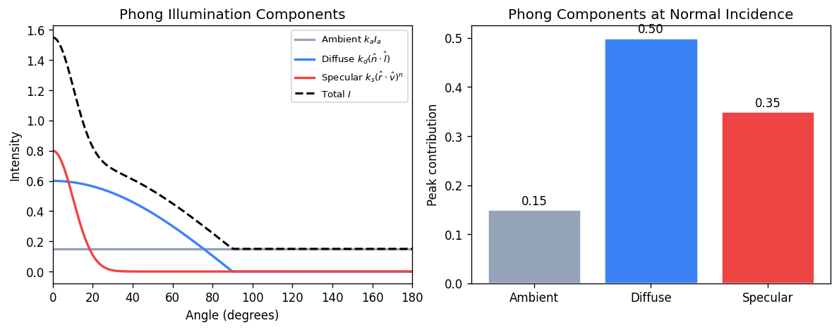
12.3 Phong Illumination Model

The Phong illumination model adds a specular highlight term to model shiny surfaces:

Here \(k_a I_a\) is ambient (a constant background term), \(\hat{\mathbf{r}}\) is the perfect mirror reflection of \(\hat{\mathbf{l}}\) about \(\hat{\mathbf{n}}\), \(\hat{\mathbf{v}}\) is the view direction, and \(n\) is the shininess exponent (larger \(n\) gives a tighter, glossier highlight). The specular term peaks when the view direction aligns with the reflection direction.

The reflection vector is \(\hat{\mathbf{r}} = 2(\hat{\mathbf{n}} \cdot \hat{\mathbf{l}})\hat{\mathbf{n}} - \hat{\mathbf{l}}\).

12.4 Blinn-Phong Model

The Blinn-Phong variant replaces the reflection vector with the halfway vector \(\hat{\mathbf{h}} = (\hat{\mathbf{l}} + \hat{\mathbf{v}})/|\hat{\mathbf{l}} + \hat{\mathbf{v}}|\), giving:

Blinn-Phong is slightly cheaper (no reflection computation) and was the model used in the OpenGL fixed-function pipeline. The shininess exponents are not directly comparable — Blinn-Phong requires a larger \(n'\) to match a given Phong highlight.

12.5 Gouraud and Phong Shading

Gouraud shading computes the illumination model at each vertex and interpolates the resulting colours across the triangle. It is efficient but misses highlights that fall between vertices.

Phong shading interpolates the surface normal across the triangle and evaluates the illumination model at each fragment (pixel). This correctly captures specular highlights anywhere on the surface. Phong shading is more expensive but produces superior results, and is standard in programmable fragment shaders.

Chapter 13: Texture Mapping

13.1 Surface Textures

Texture mapping modulates surface attributes (typically diffuse colour) by looking up values from a stored image (texture). A texture is a 2D array indexed by texture coordinates \((s, t) \in [0,1]^2\). Each geometric vertex carries a texture coordinate, which is interpolated across the triangle and used at each fragment to sample the texture.

Filtering is essential to avoid aliasing artefacts. When a texture is magnified (more screen pixels than texels), bilinear interpolation smoothly blends the four nearest texels. When minified (more texels than screen pixels), mipmapping precomputes a pyramid of progressively lower-resolution versions of the texture, and the appropriate level is selected based on the screen-space derivative of the texture coordinate.

13.2 Environment (Reflection) Mapping

Environment mapping fakes mirror reflections by encoding the surrounding environment in a texture (typically a cube map or sphere map). The reflection direction at each fragment is computed and used as the texture coordinate to look up the reflected colour. This avoids the cost of true ray-traced reflections while giving a convincing approximation for convex objects in a static environment.

13.3 Bump and Normal Mapping

Bump mapping perturbs the surface normal at each fragment according to a stored height map, making a flat surface appear rough. The partial derivatives of the height map give the normal perturbation. Normal mapping stores the perturbed normal directly in a texture (in tangent space), bypassing the derivative computation and allowing more complex normal patterns. Both techniques produce convincing surface detail without adding geometry.

13.4 Solid (Procedural) Texturing

Solid texturing (3D or procedural texturing) assigns a colour as a function of the 3D position in world or object space, rather than 2D surface coordinates. Wood grain, marble, and turbulence patterns are classic examples. The Perlin noise function is widely used as a building block for procedural textures because it is smooth, band-limited, and computationally efficient.

Chapter 14: Ray Tracing

14.1 Basic Ray Tracing

Ray tracing is a rendering algorithm that simulates light by casting rays from the camera through each pixel and testing for intersections with scene geometry. The basic algorithm is:

  for each pixel (i, j):
    ray = camera.generateRay(i, j)
    colour[i][j] = trace(ray, scene)

  trace(ray, scene):
    hit = scene.intersect(ray)
    if hit:
      return shade(hit, scene)
    else:
      return background_colour

For reflections, shade recursively traces secondary rays. For shadows, a shadow ray is cast toward each light source; if it hits any opaque object, the point is in shadow.

14.2 Ray-Object Intersections

Parametric ray: \(P(t) = \mathbf{e} + t\,\hat{\mathbf{d}}\), where \(\mathbf{e}\) is the eye (origin) and \(\hat{\mathbf{d}}\) is the unit direction.

Ray-plane intersection: Given a plane \(\mathbf{n} \cdot \mathbf{p} = d\), substitute the ray equation and solve for \(t\):

Ray-sphere intersection: A sphere with centre \(\mathbf{c}\) and radius \(r\) is the solution set of \(|\mathbf{p} - \mathbf{c}|^2 = r^2\). Substituting the ray:

The discriminant \(\Delta = (\hat{\mathbf{d}}\cdot(\mathbf{e}-\mathbf{c}))^2 - (\hat{\mathbf{d}}\cdot\hat{\mathbf{d}})(|\mathbf{e}-\mathbf{c}|^2-r^2)\) determines whether the ray misses (\(\Delta<0\), is tangent (\(\Delta=0\), or intersects at two points (\(\Delta>0\).

Quadric surfaces: A general quadric \(\mathbf{p}^T A \mathbf{p} = 0\) (in homogeneous coordinates) yields a quadratic in \(t\), so the ray-quadric intersection reduces to the same quadratic formula.

Ray-triangle intersection: One approach is to find the ray-plane intersection, then test barycentric coordinates for containment in the triangle.

14.3 Constructive Solid Geometry

CSG (Constructive Solid Geometry) builds complex objects from Boolean operations (union, intersection, difference) on simpler primitives. A CSG tree records the operation at each internal node. Ray-CSG intersection computes the sorted list of ray parameter values entering and leaving each primitive, then applies interval set operations corresponding to the Boolean operator:

  Union:      intervals that are in A OR B
  Intersect:  intervals that are in A AND B
  Difference: intervals in A and NOT in B

The closest positive \(t\) in the result is the intersection.

14.4 Bounding Volumes

Testing every ray against every object is \(O(nr)\) (n objects, r rays). Bounding volume hierarchies (BVH) and spatial subdivision structures reduce this to \(O(r \log n)\) on average.

Axis-Aligned Bounding Boxes (AABB): A box defined by \([x_\min, x_\max] \times [y_\min, y_\max] \times [z_\min, z_\max]\). Ray-AABB intersection is computed by the slab method: for each axis, compute the ray parameter interval \([t_\min, t_\max]\) where the ray is inside the slab. The ray hits the box if and only if the three intervals’ intersection is non-empty.

BVH construction: Build a binary tree by recursively partitioning the set of primitives. At each node, compute the bounding box of the primitives in that subtree. To traverse, test the ray against the bounding box; if it misses, skip the subtree entirely.

Chapter 15: Shadows

15.1 Shadow Computation Overview

Shadows are essential visual cues for depth and spatial relationships. The fundamental question is: for each point on a surface, is it visible from the light source? Three main approaches are used in practice.

15.2 Projective Shadows

Projective (planar) shadows project each primitive onto a receiver plane using a perspective transform centred at the point light. The shadow shape is the projection of the object’s silhouette onto the plane. This is cheap but limited to planar receivers and point lights.

15.3 Shadow Maps

Shadow mapping uses the light’s perspective to pre-compute a depth map of the scene as seen from the light. During rendering, each fragment is transformed into the light’s coordinate space and its depth is compared to the stored depth map. If the fragment is farther from the light than the stored depth, it is in shadow.

  Pass 1: Render scene from light's viewpoint → depth map
  Pass 2: For each fragment at depth d from light:
    if d > shadowMap[proj(fragment)] + bias:
      fragment is in shadow

The bias prevents self-shadowing artefacts (a surface point should compare against shadows cast by other surfaces, not itself). Shadow maps alias due to the finite resolution of the depth map; percentage closer filtering (PCF) softens hard edges by averaging multiple depth comparisons.

15.4 Shadow Volumes

Shadow volumes (Crow, 1977) define the volumetric region behind an object that lies in shadow. Each silhouette edge of the occluder defines two rays from the light; the shadow volume is the region between those rays beyond the occluder.

The stencil buffer method renders shadow volumes in two passes. First, the scene is rendered with ambient lighting only. Then, for each shadow volume front face, increment the stencil buffer (+1 when a depth test passes); for each back face, decrement (−1). Fragments with a non-zero stencil count are in shadow. A final pass renders the lit scene only where the stencil is zero.

Carmack’s Reverse (z-fail method) handles the case where the eye itself is inside a shadow volume, which breaks the basic algorithm.

Chapter 16: Aliasing and Sampling

16.1 The Aliasing Problem

Aliasing arises when a continuous signal is sampled at too low a frequency, causing high-frequency content to appear as spurious low-frequency content. In computer graphics, it manifests as jagged edges (staircasing), shimmering fine textures, and temporal strobing in animation.

Nyquist’s theorem states that to reconstruct a signal without aliasing, one must sample at a rate of at least twice the highest frequency present in the signal. Since edges and fine geometry can produce arbitrarily high frequencies, perfect antialiasing is impossible without prefiltering.

16.2 Supersampling (Area Sampling)

The most straightforward antialiasing approach is supersampling: render at a higher resolution and average (downsample) to the output resolution. Simple uniform supersampling samples on a regular \(n \times n\) grid within each pixel, at a cost of \(n^2\) times as many ray tests.

Stochastic (jittered) sampling randomly perturbs the sample positions within each subpixel. This converts aliasing (coherent artefacts) into noise (incoherent artefacts), which is perceptually preferable because the human visual system is more tolerant of noise than regular patterns.

Weighted sampling applies a reconstruction filter (such as a Gaussian or Mitchell-Netravali filter) when combining samples, rather than box filtering (uniform averaging), to reduce ringing and improve image sharpness.

16.3 Temporal Aliasing

Motion blur samples time as well as space, averaging contributions from multiple instants within the shutter interval. This eliminates the strobing artefacts that occur when objects move more than one pixel per frame.

Chapter 17: Distribution Ray Tracing and Global Illumination

17.1 Distribution (Monte Carlo) Ray Tracing

Distribution ray tracing (Cook et al., 1984) generalises basic ray tracing by distributing rays statistically over the domains of:

• Soft shadows: multiple shadow rays distributed over the area of an area light source.
• Glossy reflection: reflected rays distributed over a cone around the mirror direction.
• Depth of field: primary rays distributed over the aperture of a lens.
• Motion blur: rays distributed over time.
• Indirect diffuse: reflected rays distributed over the hemisphere.

The Monte Carlo estimate of a surface integral is:

where samples \(x_i\) are drawn from distribution \(p\). Importance sampling chooses \(p\) proportional to \(f\) to reduce variance.

17.2 Path Tracing

Path tracing traces complete light paths from the eye to the light source by recursively sampling the hemisphere at each bounce. Each path contributes an estimate of the light arriving at the eye via that path. With enough paths, the estimate converges to the correct solution of the rendering equation.

The rendering equation (Kajiya, 1986) describes the equilibrium distribution of radiance in a scene:

where \(L_e\) is emitted radiance, \(f_r\) is the BRDF, and the integral is over the hemisphere \(\Omega\) of incoming directions.

17.3 Photon Mapping

Photon mapping (Jensen, 1996) is a two-pass algorithm:

1. Photon tracing: emit photons from light sources, tracing them through the scene by importance sampling the BRDF. Store the photons (position, direction, power) in a spatial data structure (kD-tree) when they hit diffuse surfaces.
2. Rendering: for each camera ray, estimate the irradiance at hit points by querying the \(k\) nearest photons using the kD-tree and computing a kernel density estimate.

Russian roulette terminates photon paths probabilistically without bias: at each bounce, draw a random number; if it exceeds the reflectance, terminate; otherwise continue and scale the photon power accordingly.

Photon mapping excels at caustics (focused light patterns) and interiors. Irradiance caching accelerates rendering by caching irradiance estimates at sparsely sampled points and interpolating.

17.4 Metropolis Light Transport

Metropolis light transport (MLT) uses the Metropolis-Hastings algorithm to importance-sample the space of all light paths. Instead of generating paths independently, MLT mutates existing high-contribution paths to explore nearby paths. This makes MLT efficient in scenes with difficult light transport (small light sources, complex caustics) where standard path tracing converges slowly.

Chapter 18: Radiosity

18.1 The Radiosity Equation

Radiosity models light transport between diffuse surfaces, computing the equilibrium distribution of light energy in a scene. Each surface is subdivided into patches. The radiosity \(B_i\) (power emitted per unit area) of patch \(i\) satisfies:

where \(E_i\) is the emitted radiosity, \(\rho_i\) is the diffuse reflectance, and \(F_{ij}\) is the form factor from patch \(i\) to patch \(j\).

In matrix form this is a linear system:

18.2 Form Factors

The form factor \(F_{ij}\) represents the fraction of light leaving patch \(i\) that arrives at patch \(j\) by direct line of sight:

where \(\theta_i, \theta_j\) are the angles of the line connecting the two surface elements relative to their respective normals, \(r\) is the distance, and \(V(x,y)\) is 1 if the two points are mutually visible and 0 otherwise.

The hemi-cube method approximates form factors by rendering the scene from each patch’s perspective onto the five faces of a hemi-cube, then weighting the projected pixels by precomputed delta form factors.

18.3 Progressive Refinement

Because the radiosity system is large (one equation per patch), direct solution is expensive. Progressive refinement iteratively shoots the energy from the brightest patch to all others, updating radiosities after each step. This is a Gauss-Seidel-like iteration that converges to the solution and provides a series of increasingly accurate approximations viewable in real time.

Chapter 19: Procedural Geometry

19.1 Fractal Landscapes

Fractal terrain generation creates realistic mountain landscapes through recursive refinement. The midpoint displacement algorithm starts with a single quad and recursively subdivides each quad into four, displacing the newly introduced midpoints by a random amount proportional to a decreasing scale factor \(2^{-H \cdot i}\), where \(H\) controls the roughness (Hurst exponent) and \(i\) is the refinement level. The statistical self-similarity of the result gives a fractal dimension related to \(H\).

19.2 L-Systems

L-systems (Lindenmayer systems) are a parallel rewriting formalism for modelling self-similar structures like plants. An L-system has an alphabet, a set of production rules, and an axiom (starting string). At each generation, every symbol in the current string is simultaneously replaced by its production. The resulting string is interpreted by a turtle graphics system to produce a 3D model.

For example, a simple bracketed L-system:

  Axiom: F
  Rule:  F → F[+F]F[-F]F
  Interpretation: F = draw, + = turn left, - = turn right,
                  [ = push state, ] = pop state

19.3 Context-Free Building Grammars

Context-free grammars for buildings generalise L-systems to 3D volumetric subdivision. A starting volume is split recursively according to grammar rules (split horizontally, split vertically, assign façade texture, place window). This approach can generate enormous diversity of building styles from a small set of grammar rules.

19.4 Particle Systems

Particle systems model phenomena like fire, smoke, explosions, and waterfalls as large numbers of simple particles with individual physics (position, velocity, acceleration, lifetime). The system is defined by:

• Birth: particles are generated at emitter locations with random initial parameters.
• Dynamics: each particle follows a simple simulation (Newtonian motion with gravity and drag).
• Death: particles are removed when their lifetime expires.
• Rendering: each particle is rendered as a small billboard sprite or a point.

Chapter 20: Polyhedral Data Structures

20.1 Simple Face List

The simplest polyhedral representation stores a list of vertices (positions) and a list of polygonal faces (index lists into the vertex array). This simple face list is compact and easy to render but makes it difficult to answer adjacency queries such as “which faces share this edge?” or “what are the neighbouring vertices of this vertex?”

20.2 Generalized Polyhedral Structure

A more capable representation adds adjacency information. A vertex stores its position and a list of incident faces. A face stores its vertex indices and a list of adjacent faces. This allows efficient traversal of the mesh topology.

20.3 Euler’s Formula

For a closed, orientable polyhedron of genus \(G\) (number of handles) and \(C\) connected components with \(H\) holes (boundary loops), Euler’s formula relates vertices \(V\), edges \(E\), and faces \(F\):

For a simple closed convex polyhedron (no holes, no handles, one component): \(V - E + F = 2\) (the classic Euler formula).

20.4 Winged-Edge and Half-Edge Structures

The winged-edge data structure explicitly stores every edge as a record that references its two endpoint vertices, its two adjacent faces, and its four wing edges (the adjacent edges in clockwise and counter-clockwise order around each face). This supports all topological traversals in constant time per operation.

The half-edge (or DCEL — doubly-connected edge list) structure splits each edge into two directed half-edges, one for each adjacent face. Each half-edge stores a reference to its origin vertex, its twin half-edge (the one going in the opposite direction), its face, and the next and previous half-edges around the face. The half-edge structure is somewhat simpler to implement than winged-edge while supporting the same traversal operations.

Chapter 21: Mesh Compression and LOD

21.1 Triangle Strips

Triangle strips reduce the per-vertex overhead of transmitting geometry to the GPU. A strip of \(n\) triangles sharing edges is encoded as a sequence of \(n+2\) vertices rather than \(3n\). Automatically partitioning a mesh into strips (tristripping) reduces bandwidth by approximately 2–3×.

21.2 Progressive Meshes

Progressive meshes (Hoppe, 1996) represent a mesh at multiple levels of detail via a sequence of edge collapse operations. An edge collapse removes one edge of the mesh by merging its two endpoint vertices into one, eliminating two triangles. The inverse operation, vertex split, inserts a new vertex and restores the two faces. A stream of vertex splits can reconstruct the mesh at any desired level of detail, enabling smooth geomorphing (continuous LOD transitions with no popping).

21.3 Geometry Compression

Geometry compression exploits spatial coherence in meshes to reduce storage. Positions are quantised to a bounded number of bits and encoded as delta values relative to neighbours. Normal vectors are discretised over the sphere. Stripification and parallelogram prediction (predicting the next vertex position from the previous three) further reduce bit rates.

Chapter 22: Curves and Splines

22.1 Parametric Curves

A parametric curve is a function \(\mathbf{p}(t) = (x(t), y(t), z(t))\) for \(t \in [0,1]\). Polynomial curves are the most common because they are smooth and easy to evaluate. The challenge is to specify a curve intuitively (by a small number of control points) while maintaining desired smoothness properties.

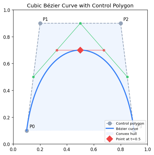
22.2 Bézier Curves

A Bézier curve of degree \(n\) is defined by \(n+1\) control points \(\mathbf{p}_0, \ldots, \mathbf{p}_n\):

where \(B_i^n(t) = \binom{n}{i} t^i (1-t)^{n-i}\) are the Bernstein polynomials. Key properties: the curve passes through the first and last control points, lies in the convex hull of all control points (convex hull property), and the tangent at the endpoints is parallel to the first/last edge of the control polygon.

The de Casteljau algorithm evaluates a Bézier curve by repeated linear interpolation:

After \(n\) rounds, \(\mathbf{p}_0^n(t) = \mathbf{p}(t)\). The intermediate points also provide a subdivision: the original curve splits at \(t\) into two Bézier curves.

22.3 Continuity Conditions

When joining curve segments, the continuity at the junction determines smoothness:

• C0: the curves share an endpoint (positions match).
• C1: the tangent vectors match in direction and magnitude.
• C2: the second derivatives match (curvature continuity).
• G1 (geometric C1): tangents match in direction only (allowing different magnitudes).

22.4 Catmull-Rom Splines

A Catmull-Rom spline interpolates through all control points. The tangent at each control point \(\mathbf{p}_i\) is set to \(\frac{1}{2}(\mathbf{p}_{i+1} - \mathbf{p}_{i-1})\\). Catmull-Rom splines are C1, automatically smooth, and require no separate tangent specification from the user.

22.5 B-Splines

B-splines are piecewise polynomial curves defined over a knot vector. They offer local control (moving one control point affects only nearby curve segments), and can achieve C2 continuity with cubic pieces. The NURBS (Non-Uniform Rational B-Splines) generalisation allows the exact representation of conics (circles, ellipses) and is the industry standard for CAD modelling.

Chapter 23: Surfaces

23.1 Tensor Product Patches

A tensor product patch is a surface defined by a grid of control points \(\mathbf{p}_{ij}\). The surface is evaluated at parameter \((s, t)\) by applying the curve basis in each direction:

A bicubic Bézier patch uses a 4×4 grid of control points and Bernstein basis in each direction. Sixteen control points define a smooth surface patch.

23.2 Triangular Bézier Patches

Triangular Bézier patches (simplex patches) parameterise a surface over a triangular domain using barycentric coordinates \((u, v, w)\) with \(u+v+w=1\). They fill triangular gaps in meshes where rectangular patches leave holes.

23.3 Subdivision Surfaces

Subdivision surfaces define smooth surfaces as the limit of a recursive refinement process. Starting from a coarse control mesh, refinement rules split and average vertices repeatedly. The limit surface is smooth everywhere (or everywhere except at extraordinary vertices).

Catmull-Clark subdivision generalises bi-cubic B-splines to arbitrary topology meshes. Its rules for face points, edge points, and vertex points at each refinement level produce a C2 surface everywhere except at extraordinary vertices (vertices with valence ≠ 4).

Loop subdivision targets triangle meshes and generalises cubic box splines, producing a C2 surface except at extraordinary vertices.

23.4 Implicit Surfaces and Marching Cubes

An implicit surface is the zero set of a scalar field \(F(\mathbf{p}) = 0\). Radial basis function (RBF) surfaces construct \(F\) as a sum of radially symmetric functions centred at scattered sample points, fitting the surface to point cloud data.

Marching cubes polygonises an implicit surface by marching a grid of cubes through space. For each cube, the signs of \(F\) at the eight corners determine a case in a lookup table of 256 configurations (reduced to 15 by symmetry), giving the local triangulation. Edge intersections are interpolated for sub-voxel accuracy.

Chapter 24: Wavelets

24.1 Haar Wavelets

The Haar wavelet is the simplest wavelet basis. Given a signal of length \(n = 2^k\), one step of the Haar transform computes for each pair of adjacent values their average (low-pass / scaling coefficient) and their half-difference (high-pass / wavelet coefficient):

Iterating this transform on the scaling coefficients produces a multi-resolution decomposition. The wavelet coefficients encode detail at each scale. Zeroing small coefficients provides compression.

24.2 2D Image Compression

Applying the 1D Haar transform separately in horizontal and vertical directions decomposes a 2D image into four quadrants: LL (low-low, the thumbnail), LH (horizontal detail), HL (vertical detail), and HH (diagonal detail). Recursively decomposing the LL quadrant produces a full multi-resolution pyramid. Discarding or quantising small-magnitude detail coefficients achieves image compression with controlled quality loss, similar to the JPEG-2000 approach.

Chapter 25: Non-Photorealistic Rendering

25.1 Painterly Rendering

Non-photorealistic rendering (NPR) aims to produce images with the aesthetic of traditional media — watercolour, pen-and-ink, pencil, oil painting — rather than photorealistic images. Painterly rendering represents a scene as a collection of brush strokes, each positioned and oriented to capture local colour and gradient information. The Hertzmann painterly rendering algorithm places strokes from coarse to fine: begin with large strokes for overall colour, then overlay progressively smaller strokes for detail in high-gradient regions.

25.2 Watercolour and Pencil Simulation

Watercolour simulation models the physics of wet-on-wet pigment diffusion, wet-on-dry granulation, edge darkening (the wet-edge effect), and bleeding at paper boundaries. Pencil simulation uses a paper texture model (paper fibres elevate above recesses) combined with a stroke model that deposits pigment only on the elevated fibres.

25.3 Pen-and-Ink and Hatching

Pen-and-ink rendering produces line drawings with hatching and cross-hatching for shading. Strokes are placed with density proportional to local darkness. Silhouette edges — edges where one adjacent face is front-facing and the other is back-facing — are the most important lines in a line drawing. They convey the 3D shape of the object.

25.4 Toon (Cel) Shading

Toon shading replicates the flat colour regions and dark outlines of hand-drawn animation. The diffuse component is quantised into a small number of discrete values (typically 2–3 bands) via a step function or a 1D lookup texture indexed by the diffuse dot product. Outlines are rendered as a separate pass: either by rendering the back-face-only geometry slightly enlarged (shell method) or by detecting edges in screen space via a Sobel filter on the depth buffer.

Chapter 26: Volume Rendering

26.1 Volume Data

Volume rendering visualises 3D scalar fields, such as medical CT/MRI scan data (voxel grids of density values) or simulation outputs (temperature, pressure). Each voxel stores a scalar value; the rendering algorithm must determine what colour and opacity to assign each voxel and how to integrate contributions along view rays.

26.2 Segmentation and Classification

Segmentation partitions voxels into tissue types (bone, soft tissue, air) or other meaningful classes. Classification assigns transfer functions: each scalar value (or range) maps to a colour and opacity (alpha) via a lookup table (LUT) or transfer function. This step allows selective visualisation — e.g., rendering only bone while making soft tissue transparent.

26.3 Resampling and Gradients

When a view ray passes through the volume at an oblique angle, it must sample the volume at non-integer positions. Trilinear interpolation (or higher-order resampling) interpolates the eight nearest voxel values for a continuous scalar field. Gradient estimation computes the surface normal at each voxel position (e.g., via central differences) for shading.

26.4 Compositing

Along each view ray, voxel contributions are combined by the front-to-back compositing (Porter-Duff over operation):

Once accumulated opacity reaches 1, further voxels along the ray can be skipped (early ray termination). Maximum Intensity Projection (MIP) is an alternative that simply displays the maximum voxel value along each ray, producing bright vascular images in medical imaging.

Chapter 27: Animation

27.1 Keyframing and Interpolation

Keyframe animation specifies the state of an object (position, orientation, scale) at discrete keyframe times and interpolates in between. Smooth interpolation uses splines (e.g., Catmull-Rom) through the keyframe values. Ease-in / ease-out (slow at start and end) is achieved by choosing a non-uniform parameterisation of the spline.

Arc-length parameterisation reparameterises the spline so that equal parameter increments correspond to equal distances along the curve, ensuring constant-speed motion.

27.2 Euler Angles, Gimbal Lock, and Quaternion Animation

When animating orientation, naïve interpolation of Euler angles produces unnatural trajectories and can pass through gimbal lock configurations. Quaternion interpolation via SLERP avoids these problems and produces smooth, constant-angular-velocity rotation.

27.3 Skeletons and Skinning

A skeleton (articulated figure) is a tree of rigid bones connected at joints. Each bone has a local transformation relative to its parent. Transforming the root propagates through the hierarchy via forward kinematics. Skinning (linear blend skinning) deforms a surface mesh by weighting each vertex’s position as a blend of the transformations of the nearby bones.

27.4 Forward and Inverse Kinematics

Forward kinematics computes end-effector position from joint angles (a straightforward evaluation of the kinematic chain). Inverse kinematics (IK) computes the joint angles that place an end-effector at a target position, a more complex numerical optimisation problem. The Jacobian of the kinematic chain maps joint angle velocities to end-effector velocity; IK solvers based on the Jacobian pseudo-inverse iterate toward the solution.

27.5 Free-Form Deformation

Free-Form Deformation (FFD) deforms a 3D object by embedding it in a lattice of control points and deforming the lattice. Each point in the object is expressed in the lattice’s parameter space; when the lattice is deformed, the object deforms smoothly. FFD is widely used for organic modelling and character animation.

27.6 Spring-Mass Physics

Spring-mass simulation models cloth and deformable objects as particles connected by springs. Newton’s second law gives the dynamics:

where \(k_{ij}\) is the spring stiffness, \(L_{ij}\) is the rest length, and \(\mathbf{f}_\text{ext}\) are gravity, wind, and contact forces. Integration (Euler, Verlet, or implicit methods) advances the simulation over time.

27.7 Morphing

Morphing smoothly transforms one shape into another. For 2D images, morphing requires defining a correspondence between features in the two images (control points or mesh vertices), warping both images toward an intermediate shape, and cross-dissolving the colours.

27.8 Motion Capture

Motion capture records the movement of a real human or animal by tracking markers attached to the body. The captured marker trajectories are mapped to a skeleton, providing naturalistic animation data. Post-processing fills gaps (occluded markers) and retargets the motion to differently-proportioned characters.

27.9 Flocking and Behavioural Animation

Reynolds’ flocking model (Boids, 1987) produces emergent flock behaviour from three simple local rules applied to each agent:

1. Separation: steer away from nearby neighbours to avoid crowding.
2. Alignment: steer toward the average heading of nearby neighbours.
3. Cohesion: steer toward the average position (centre of mass) of nearby neighbours.

Combined, these rules produce realistic flocking, herding, and schooling behaviour with no central control.

Chapter 28: Computational Geometry

28.1 Spatial Data Structures

Spatial data structures organise geometric data to support efficient queries such as nearest-neighbour search, range queries, and ray-intersection tests.

A quadtree recursively divides a 2D region into four equal quadrants. A octree does the same in 3D, dividing into eight octants. Both support approximate nearest-neighbour queries in \(O(\log n)\) time on average.

A kD-tree recursively partitions space by axis-aligned hyperplanes chosen to split the point set roughly in half along the longest axis. A kD-tree supports exact nearest-neighbour and range queries in \(O(\log n)\) time on average. It is the standard data structure for photon maps and for range queries in point cloud processing.

A BSP tree (Binary Space Partition) partitions space by arbitrary planes rather than axis-aligned ones. A convex partition of the scene encoded in a BSP tree can be traversed in exact back-to-front or front-to-back order with respect to any viewpoint, making BSPs historically important for the painter’s algorithm and portal rendering in early game engines.

28.2 Convex Hull

The convex hull of a point set is the smallest convex set containing all points. In 2D, the convex hull is a polygon; in 3D, a convex polyhedron. Graham scan computes the 2D convex hull in \(O(n \log n)\) by sorting points by polar angle and maintaining a stack of hull vertices.

28.3 Voronoi Diagrams and Delaunay Triangulation

The Voronoi diagram of a point set partitions the plane into cells, one per point, where each cell contains all locations closer to its point than to any other. Voronoi diagrams are useful for proximity queries, path planning, and territorial modelling.

The Delaunay triangulation is the dual of the Voronoi diagram: it connects points by edges whenever their Voronoi cells share a boundary. The Delaunay triangulation maximises the minimum angle among all triangulations of the point set, producing well-shaped triangles that avoid degenerate slivers.

The flip algorithm constructs the Delaunay triangulation incrementally: when adding a new point, edges that violate the Delaunay condition (the circumcircle of a triangle contains the new point) are flipped, and the process repeats until all edges satisfy the condition.

Chapter 29: More on Shaders and GLSL

29.1 Vertex Shader Details

The vertex shader receives per-vertex data as attribute variables and per-draw-call constants as uniform variables. It must write gl_Position (the clip-space position) and optionally write per-vertex varying variables that are interpolated across the primitive and passed to the fragment shader.

A typical vertex shader:

attribute vec3 aPosition;
attribute vec3 aNormal;
attribute vec2 aTexCoord;
uniform mat4 uMVP;
uniform mat3 uNormalMatrix;
varying vec3 vNormal;
varying vec2 vTexCoord;

void main() {
    gl_Position = uMVP * vec4(aPosition, 1.0);
    vNormal = normalize(uNormalMatrix * aNormal);
    vTexCoord = aTexCoord;
}

29.2 Fragment Shader Details

The fragment shader receives interpolated varying values from the vertex shader, accesses uniform textures via sampler2D uniforms, and writes gl_FragColor (the output pixel colour).

A typical Phong fragment shader:

uniform sampler2D uTexture;
uniform vec3 uLightDir;
uniform vec3 uViewDir;
varying vec3 vNormal;
varying vec2 vTexCoord;

void main() {
    vec3 n = normalize(vNormal);
    float diff = max(dot(n, uLightDir), 0.0);
    vec3 h = normalize(uLightDir + uViewDir);
    float spec = pow(max(dot(n, h), 0.0), 64.0);
    vec4 texColor = texture2D(uTexture, vTexCoord);
    gl_FragColor = texColor * (0.1 + 0.7*diff) + vec4(1.0)*spec*0.2;
}

29.3 Normal Mapping in GLSL

Normal mapping reads a perturbed normal from a texture (stored in tangent space: RGB → XYZ in \([-1,1]^3\) and transforms it to world space using a tangent-space basis (TBN matrix) computed per vertex.

Chapter 30: Advanced Illumination Models

30.1 The BRDF

The Bidirectional Reflectance Distribution Function (BRDF) \(f_r(\omega_i, \omega_o)\) quantifies how much light arriving from direction \(\omega_i\) is reflected in direction \(\omega_o\). The BRDF is the fundamental quantity in physically based rendering. Key properties:

• Helmholtz reciprocity: \(f_r(\omega_i, \omega_o) = f_r(\omega_o, \omega_i)\).
• Energy conservation: \(\int_\Omega f_r(\omega_i, \omega_o) \cos\theta_o\, d\omega_o \le 1\).

The Phong model can be rewritten as a BRDF. Physically based BRDFs (such as Cook-Torrance) derive the specular term from microfacet theory.

30.2 Cook-Torrance Microfacet Model

The Cook-Torrance model treats a surface as a collection of microscopic mirror-like facets. The specular BRDF is:

where:

• \(D(\mathbf{h})\) is the normal distribution function (fraction of microfacets with normal aligned with the halfway vector \(\mathbf{h}\),
• \(F(\theta_d)\) is the Fresnel term (fraction of light reflected vs. refracted at each microfacet),
• \(G(\omega_i, \omega_o)\) is the geometric attenuation (accounting for masking and shadowing between microfacets).

30.3 Subsurface Scattering

Subsurface scattering (SSS) occurs when light penetrates a translucent material (skin, wax, marble, milk) and scatters inside before exiting. Standard surface shading models cannot capture SSS, which gives skin its characteristic soft glow. Rendering SSS requires either volumetric path tracing or efficient approximations such as dipole diffusion (Jensen et al., 2001).

Chapter 31: Implicit Surfaces and Special Topics

31.1 Algebraic Surfaces

Algebraic surfaces are defined by polynomial equations \(F(x,y,z)=0\). The degree of the polynomial determines the complexity: degree-1 gives a plane, degree-2 a quadric (sphere, ellipsoid, paraboloid, hyperboloid), degree-4 a quartic, etc. Algebraic surfaces can be rendered by direct ray-implicit intersection solving.

31.2 A-Patches (Algebraic Patches)

A-patches are surface patches defined by implicitly bounding a polynomial inequality \(F(\mathbf{p}) \ge 0\) within a simplex domain. They can represent complex smooth shapes and blend naturally. A-patches avoid the need for explicit parameterisation of the surface.

31.3 Depth of Field

Depth of field arises from the finite aperture of a lens: points at the focal distance are sharp while points closer or farther are blurred by a circle of confusion. In distribution ray tracing, depth of field is simulated by distributing primary rays across the lens aperture and converging them at the focal plane.

Chapter 32: Selected Rendering Techniques

32.1 Image-Based Rendering

Image-based rendering (IBR) synthesises novel views of a scene from a set of captured photographs rather than a geometric model. The light field encodes the radiance along every ray in free space using a 4D parameterisation (two plane coordinates × two direction coordinates). Rendering a novel view requires sampling the light field, either by interpolation or by lookup in a precomputed table.

View morphing and image warping are simpler forms of IBR that synthesise intermediate views between two captured images by correspondence-based warping.

32.2 Level of Detail (LOD) and Culling

Efficient rendering of large scenes requires both LOD (rendering less detailed versions of distant objects) and culling (not rendering objects outside the view frustum or behind large occluders).

Frustum culling tests each object’s bounding volume against the six frustum planes; if the bounding volume is completely outside any plane, the object is invisible and can be skipped.

Occlusion culling skips objects that are behind large occluders. Hardware occlusion queries allow the GPU to test whether any samples of a bounding box would pass the depth test, indicating whether the object behind it is worth rendering.

Portal rendering uses the fact that indoor scenes have walls that occlude large portions of the world; only the geometry visible through open doors and windows (portals) needs to be rendered.

32.3 Deferred Shading

Deferred shading separates geometry processing from lighting computation. In a first pass (G-buffer pass), the scene is rendered and per-pixel surface properties (position, normal, albedo, material parameters) are written into a collection of render targets (the G-buffer). In a second pass (lighting pass), each light source is processed as a screen-space operation that reads the G-buffer and accumulates the light contribution. Deferred shading makes the cost of adding lights proportional to the lit screen area rather than the scene complexity, at the cost of losing transparency and requiring large G-buffer memory.

Chapter 33: Assignments Overview

The CS488/688 programming assignments build progressively on the rendering pipeline and graphics concepts:

Assignment 0: Introduction to OpenGL and GLSL — Set up the development environment, compile and run a sample OpenGL/GLSL application, and understand the basic structure of a shader program.

Assignment 1: Image Manipulation — Implement basic 2D image operations: drawing primitives, colour manipulation, and region filling in a software rasteriser.

Assignment 2: 3D Transformations — Implement the 3D transformation pipeline, including model, view, and projection matrices. Visualise a 3D scene with user-controlled camera navigation.

Assignment 3: Ray Tracer — Implement a basic recursive ray tracer with:

• Rays through pixels (perspective projection),
• Phong illumination with ambient, diffuse, and specular components,
• Shadows via shadow rays to multiple light sources,
• Reflections via recursive secondary rays,
• At minimum: spheres and polygonal meshes as primitive types.

Assignment 4: Ray Tracer (Extended) — Extend the ray tracer with additional features selected from a menu including:

• texture mapping, bump/normal mapping,
• refraction (Snell’s law),
• supersampling (uniform or stochastic),
• constructive solid geometry (CSG),
• procedural textures (e.g., Perlin noise),
• depth of field,
• glossy reflection,
• soft shadows (area lights),
• acceleration (BVH or spatial subdivision).

Assignment 5: Hierarchical Modelling / Animation — Build a hierarchical scene graph using articulated joints. Animate the scene either via keyframe interpolation or forward kinematics on a character skeleton. Demonstrate the matrix stack through a non-trivial multi-level hierarchy.

Students are expected to demonstrate mastery of the rendering equation and its approximate solutions, proficiency in OpenGL/GLSL shader programming, and practical experience constructing a complete ray tracer.

These notes were prepared from lecture material for CS488/688 Introduction to Computer Graphics, University of Waterloo, Spring 2020.