Theorem 1.1. The probability that the algorithm outputs a minimum cut is at least \( \frac{2}{n(n-1)} \), where \( n = |V| \).

Proof. Let \( F \) be a minimum cut with \( k = |F| \) edges. If we never contract an edge of \( F \), the algorithm succeeds. What is the probability that an edge of \( F \) is contracted in the \( i \)-th iteration?

By the observation above, the minimum cut in the \( i \)-th iteration is still at least \( k \). This implies that every vertex has degree at least \( k \) (otherwise we could disconnect a single vertex by removing fewer than \( k \) edges). Therefore, the number of edges in the \( i \)-th iteration is at least \( (n - i + 1) \cdot k / 2 \).

Since we pick a random edge to contract, the probability of picking an edge in \( F \) is at most

The probability that \( F \) survives until the end is at least

1.4 Boosting Success Probability

A natural approach is to repeat the algorithm independently many times and return the smallest cut found. If we repeat \( t \) times, the failure probability is at most

Using the inequality \( 1 - x \leq e^{-x} \) (which follows from the Taylor expansion of \( e^{-x} \)), this is at most \( e^{-2t/(n(n-1))} \). Setting \( t = 10 \cdot \binom{n}{2} \) drives the failure probability below \( 2^{-20} \).

Running time. A single execution can be implemented in \( O(n^2) \) time (an exercise in data structures), giving a total time complexity of \( O(n^4) \).

Improving the running time. The key observation is that the failure probability is only large near the end of an execution — in the early iterations, the survival probability per step is very high. This suggests repeating only the later iterations while sharing the early ones. This leads to the Karger–Stein algorithm (1993), which achieves \( \tilde{O}(n^2) \) running time by branching into independent repetitions after contracting down to \( n / \sqrt{2} \) vertices. See Motwani–Raghavan, Section 10.2, for details.

1.5 Combinatorial Consequences

An elegant corollary of Theorem 1.1 is that any undirected graph has at most \( \binom{n}{2} = O(n^2) \) minimum cuts. This follows because each minimum cut survives with probability \( \Omega(1/n^2) \), and the events that two different minimum cuts survive are disjoint (the algorithm can output at most one cut). This is a nontrivial structural statement that is surprisingly difficult to prove by other means.

The algorithm can also be extended to find a minimum \( k \)-cut (partitioning the vertices into \( k \) nonempty groups while minimizing the number of crossing edges) in \( n^{O(k)} \) time. Note that the minimum \( k \)-cut problem is NP-hard when \( k \) is part of the input.

1.6 Probability Review

Before proceeding, we recall the essential probability concepts used throughout the course.

The sample space \( \Omega \) is the set of all possible outcomes. An event \( E \subseteq \Omega \) has probability \( \Pr(E) = \sum_{s \in E} \Pr(s) \). The axioms require \( 0 \leq \Pr(E) \leq 1 \), \( \Pr(\Omega) = 1 \), and countable additivity for disjoint events.

The union bound states \( \Pr\left(\bigcup_i E_i\right) \leq \sum_i \Pr(E_i) \). The inclusion-exclusion principle gives the exact probability by alternating sums of intersection probabilities.

A random variable \( X \) is a function from \( \Omega \) to \( \mathbb{R} \). Two random variables are independent if \( \Pr(X = x \cap Y = y) = \Pr(X = x) \cdot \Pr(Y = y) \) for all \( x, y \).

The expectation \( E[X] = \sum_i i \cdot \Pr(X = i) \) is linear: \( E\left[\sum_i X_i\right] = \sum_i E[X_i] \), even for dependent variables. This linearity of expectation is one of the most powerful tools in probabilistic analysis and will be used repeatedly.

Section 1.2: Concentration Inequalities

Tail inequalities, also called concentration inequalities, bound the probability that a random variable deviates far from its expected value. They allow us to show that randomized algorithms behave as expected with high probability — almost deterministically. These are fundamental tools that we will use throughout the course.

2.1 Markov’s Inequality

The simplest tail inequality requires only the expected value.

Theorem 2.1 (Markov’s Inequality). Let \( X \) be a non-negative random variable. Then for any \( a > 0 \),

Proof. \( E[X] = \sum_i i \cdot \Pr(X = i) \geq \sum_{i \geq a} i \cdot \Pr(X = i) \geq a \cdot \Pr(X \geq a) \). \( \square \)

Example (Quicksort). The expected runtime of randomized quicksort is \( 2n \ln n \). Markov’s inequality tells us that the runtime exceeds \( 2cn \ln n \) with probability at most \( 1/c \).

Example (Coin flips). If we flip \( n \) fair coins, the expected number of heads is \( n/2 \). Markov’s inequality gives \( \Pr(\text{heads} \geq 3n/4) \leq 2/3 \) — a rather weak bound that we will soon improve dramatically.

Markov’s inequality is most useful when we have no information beyond the expected value, or when the random variable is too complicated to analyze further. It is tight: consider a random variable that equals \( a \) with probability \( \mu/a \) and 0 otherwise.

2.2 Chebyshev’s Inequality

To obtain sharper bounds, we use the variance \( \text{Var}[X] = E[(X - E[X])^2] = E[X^2] - E[X]^2 \), which measures how spread out a distribution is. The standard deviation is \( \sigma(X) = \sqrt{\text{Var}[X]} \).

Two useful facts (whose proofs are exercises):

• \( \text{Var}[X + Y] = \text{Var}[X] + \text{Var}[Y] + 2\text{Cov}(X, Y) \).
• If \( X \) and \( Y \) are independent, then \( \text{Var}[X + Y] = \text{Var}[X] + \text{Var}[Y] \).

Theorem 2.2 (Chebyshev’s Inequality). For any random variable \( X \) and any \( a > 0 \),

Proof. Apply Markov’s inequality to the non-negative random variable \( (X - E[X])^2 \):

Example (Coin flips revisited). For \( n \) independent fair coin flips with \( X = \) number of heads, each indicator \( X_i \) has variance \( p(1-p) = 1/4 \). By independence, \( \text{Var}(X) = n/4 \). Chebyshev gives

This is already much better than Markov’s bound of \( 2/3 \), and it improves with \( n \).

2.3 Chernoff Bounds

When \( X \) is a sum of independent random variables, we can obtain exponentially small tail bounds. The key idea is to apply Markov’s inequality not to \( X \) itself, but to the moment generating function \( e^{tX} \):

There are two reasons this approach is powerful:

1. The function \( M_X(t) = E[e^{tX}] \) encodes all moments of \( X \) (it is the moment generating function), so Markov’s inequality applied to \( e^{tX} \) exploits all moment information simultaneously.

2. If \( X = X_1 + X_2 \) with \( X_1, X_2 \) independent, then \( E[e^{tX}] = E[e^{tX_1}] \cdot E[e^{tX_2}] \), so the moment generating function factorizes — making it easy to compute for sums of independent variables.

Heterogeneous Coin Flips

Let \( X_1, \ldots, X_n \) be independent random variables with \( X_i = 1 \) with probability \( p_i \) and \( X_i = 0 \) otherwise. Let \( X = \sum_{i=1}^n X_i \) and \( \mu = E[X] = \sum_{i=1}^n p_i \).

Then

where we used \( 1 + x \leq e^x \).

Theorem 2.3 (Chernoff Bounds). In the heterogeneous coin-flipping setting:

Proof of (i). By the calculation above, \( \Pr(X \geq (1+\delta)\mu) \leq e^{\mu(e^t - 1)} / e^{t(1+\delta)\mu} \). Minimizing over \( t \) by elementary calculus gives \( t = \ln(1+\delta) \), yielding the bound. \( \square \)

Part (ii) follows from the inequality \( e^\delta / (1+\delta)^{1+\delta} \leq e^{-\delta^2/3} \) for \( \delta \in (0, 1) \), verified by analyzing the function \( f(\delta) = \delta - (1+\delta)\ln(1+\delta) + \delta^2/3 \).

Similar bounds hold for the lower tail by setting \( t < 0 \) in the moment generating function argument.

The Coin-Flip Example Completed

For \( n \) fair coin flips, \( \mu = n/2 \). Setting \( \delta = \sqrt{60/n} \) gives \( \Pr(|X - n/2| \geq \sqrt{15n}) \leq 2e^{-10} \). With high probability, the number of heads lies within \( O(\sqrt{n \log n}) \) of its expectation — this \( \sqrt{n \log n} \) scale appears repeatedly in the analysis of randomized algorithms.

For the specific bound on \( 3n/4 \) heads: Chernoff gives \( \Pr(X \geq 3n/4) \leq e^{-n/24} \), which is exponentially small in \( n \). Compare this with Markov’s \( 2/3 \) and Chebyshev’s \( 4/n \).

Extensions

Hoeffding’s extension. The same Chernoff bounds hold when each \( X_i \) takes values in \( [0, 1] \) (not just \( \{0, 1\} \)). This follows because \( e^{tx} \) is convex, so \( E[e^{tX_i}] \leq 1 + p_i(e^t - 1) \) by the chord inequality.

Negatively correlated variables. Chernoff bounds also apply when the variables are negatively correlated, because \( E[e^{t(X_1 + X_2)}] \leq E[e^{tX_1}] \cdot E[e^{tX_2}] \) still holds. This is useful, for example, in analyzing random spanning trees, where the events that two edges appear are negatively correlated.

2.4 Probability Amplification

Concentration inequalities provide a systematic way to boost the success probability of randomized algorithms.

One-sided error. If a randomized algorithm is always correct when it answers NO but correct with probability \( p \) when it answers YES, we simply repeat \( k \) times or until it says NO. The failure probability drops to \( (1-p)^k \). For constant \( p \), repeating \( O(\log n) \) times drives the failure probability to \( O(1/n) \).

Two-sided error. If the algorithm gives the correct answer with probability 0.6, we repeat \( k \) times and output the majority answer. By the Chernoff bound, the majority is wrong with probability at most \( e^{-k/120} \). Again, \( k = O(\log n) \) suffices for failure probability \( O(1/n) \).

This \( O(\log n) \) amplification cost is another recurring quantity throughout the course.

Section 1.3: Applications of Tail Inequalities

We now apply concentration inequalities to two beautiful and important problems: graph sparsification and dimension reduction. Both demonstrate a recurring theme — random sampling preserves structure surprisingly well.

3.1 Graph Sparsification

Given an undirected graph \( G = (V, E) \) with edge weights \( w(e) \), we want a sparse graph \( H \) that approximates the cut structure of \( G \).

Definition 3.1 (\( \varepsilon \)-cut sparsifier). We say \( H = (V, F) \) is an \( \varepsilon \)-cut sparsifier of \( G = (V, E) \) if for all \( S \subseteq V \),

where \( \delta_G(S) \) denotes the set of edges crossing the cut \( (S, V \setminus S) \).

Note that \( G \) and \( H \) share the same vertex set but may have different edge sets and weights. The question is: how few edges can \( H \) have while still preserving all \( 2^n \) cut values?

Uniform Sampling under Large Minimum Cut

We start with a simple but instructive result that assumes the input graph is unweighted with minimum cut value \( c = \Omega(\log n) \).

Algorithm. Set a sampling probability \( p \). For every edge \( e \in E(G) \), independently include \( e \) in \( H \) with probability \( p \), assigning it weight \( 1/p \).

The idea is to set expectations right: we sample a \( p \)-fraction of edges and scale their weights by \( 1/p \), so that the expected weight of each cut in \( H \) equals its weight in \( G \). The challenge is ensuring that all cuts are simultaneously well-approximated.

Theorem 3.2 (Karger). Set \( p = \frac{15 \ln n}{\varepsilon^2 c} \). Then \( H \) is an \( \varepsilon \)-cut sparsifier of \( G \) with \( O(p \cdot |E|) \) edges, with probability at least \( 1 - 4/n \).

Proof. Fix a subset \( S \subseteq V \) whose cut has \( k \geq c \) edges. The number of sampled edges crossing \( S \) is a sum of independent Bernoulli variables with mean \( pk \). By the Chernoff bound,

Since \( k \geq c \), the violation probability for any single cut is at most \( n^{-5} \). But there are \( 2^n \) subsets, so a naive union bound fails. The key insight uses the combinatorial structure from Chapter 1:

Lemma 3.3. The number of cuts with at most \( \alpha c \) edges is at most \( n^{2\alpha} \).

Grouping cuts by size and applying a refined union bound:

Applications. For essentially complete graphs (\( c = \Omega(n) \)), this gives an \( \varepsilon \)-cut sparsifier with only \( O(n \log n / \varepsilon^2) \) edges — a dramatic reduction from \( \Omega(n^2) \) edges. To approximate the minimum \( s \)-\( t \) cut, sparsify first, then run an exact algorithm on the sparse graph.

Improvement by Benczur and Karger. Without the minimum-cut assumption, uniform sampling fails (e.g., a bridge edge might not be sampled). Benczur and Karger designed a non-uniform sampling algorithm where each edge is sampled with probability inversely proportional to the “strong connectivity” of its endpoints, yielding an \( \varepsilon \)-cut sparsifier with \( O(n \log n / \varepsilon^2) \) edges for any graph, constructible in near-linear time.

Near-Linear Time Minimum Cut (Sketch)

An amazing application of graph sparsification is Karger’s near-linear time algorithm for minimum cuts. The idea uses a classical result: if \( G \) is \( c \)-edge-connected, then \( G \) contains at least \( \lfloor c/2 \rfloor \) edge-disjoint spanning trees. At least one of these trees crosses a minimum cut at most twice. Finding a minimum cut that removes at most two edges from a given tree can be solved by a sophisticated dynamic programming algorithm in \( \tilde{O}(m) \) time.

The catch is that finding \( c \) edge-disjoint spanning trees takes \( O(mc) \) time, which is too slow. The solution: sparsify the graph so the minimum cut value drops to \( O(\log n) \) while preserving all cuts approximately. Now we only need \( O(\log n) \) spanning trees, and the total complexity is \( \tilde{O}(m) \).

3.2 Dimension Reduction: The Johnson–Lindenstrauss Lemma

Given \( n \) points in high-dimensional Euclidean space, can we project them to a much lower-dimensional space while approximately preserving all pairwise distances? Surprisingly, yes.

Theorem 3.4 (Johnson–Lindenstrauss Lemma). For any \( \varepsilon \in (0, 1/2) \) and any set of \( n \) points \( X = \{x_1, \ldots, x_n\} \) in \( \mathbb{R}^d \), there exists a map \( A: \mathbb{R}^d \to \mathbb{R}^k \) for \( k = O(\log n / \varepsilon^2) \) such that

for all pairs \( i, j \).

The construction is beautifully simple: let \( M \) be a \( k \times d \) matrix whose entries are independent standard Gaussians \( N(0, 1) \), and define \( A(x) = \frac{1}{\sqrt{k}} M x \).

Since \( A \) is linear, preserving distances reduces to preserving norms: it suffices to show that \( \|A(x)\|_2^2 \approx \|x\|_2^2 \) for any unit vector \( x \).

Proof sketch. Consider the special case \( x = e_1 = (1, 0, \ldots, 0) \). Then \( Me_1 \) is the first column of \( M \), a vector of \( k \) independent standard Gaussians. Its squared norm is \( \sum_{i=1}^k M_{i,1}^2 \), which has expectation \( k \). After scaling by \( 1/k \), the expected squared norm of \( A(e_1) \) is 1.

For a general unit vector \( x \), each coordinate of \( Mx \) is a linear combination of Gaussians, which is itself Gaussian with mean 0 and variance \( \|x\|_2^2 = 1 \). So the argument reduces to the special case.

The concentration bound requires a Chernoff-type inequality for chi-squared random variables (sums of squared Gaussians): \( \Pr(\|Ax\|_2^2 \geq 1 + \varepsilon) \leq e^{-k\varepsilon^2/8} \). Setting \( k = O(\log n / \varepsilon^2) \) and applying the union bound over all \( \binom{n}{2} \) pairs completes the proof.

Applications. The JL lemma enables approximate nearest-neighbor search in \( O(n \log n) \) time (down from \( O(n^2) \) with a linear scan) and approximate matrix multiplication in \( O(n^2 \log n) \) time. Note that it applies specifically to Euclidean (\( \ell_2 \)) distances.

The same result holds when \( M \) is a random \( \pm 1 \) matrix (Achlioptas), which is simpler to implement. This connection to random sign matrices will reappear when we study data streaming.

Section 1.4: Balls and Bins

The balls-and-bins model is one of the most fundamental random processes in computer science. We throw \( m \) balls independently and uniformly at random into \( n \) bins, and study the resulting distribution. This simple model underlies the analysis of hashing, load balancing, and many other applications.

4.1 Expected Number of Balls in a Bin

Let \( B_{i,j} \) be the indicator that ball \( j \) lands in bin \( i \). Then

When \( m = n \), the expected load per bin is 1. But do we expect most bins to have about one ball?

4.2 Expected Number of Empty Bins

Let \( Y_i \) be the indicator that bin \( i \) is empty. Then

using \( 1 - x \approx e^{-x} \) for small \( x \). By linearity of expectation,

When \( m = n \), roughly \( n/e \approx 0.37n \) bins are expected to be empty — more than a third! This random variable is in fact concentrated around its mean, confirming that we reliably see about 37% empty bins.

4.3 The Birthday Paradox

For what \( m \) do we expect a collision — two balls in the same bin? The probability of no collision in the first \( m \) balls is

This drops below \( 1/2 \) when \( m = \sqrt{2n \ln 2} \). For \( n = 365 \) (the classical birthday problem), this gives \( m \geq 23 \), very close to the exact answer.

The key intuition: there are \( \binom{m}{2} \) pairs of potential collisions, so we expect a collision when \( m^2 \approx n \), i.e., \( m \approx \sqrt{n} \). This square-root threshold appears throughout hashing, cryptographic attacks, and number-theoretic algorithms.

4.4 Maximum Load

When \( m = n \), what is the maximum number of balls in any bin?

The probability that a specific bin has at least \( k \) balls is at most \( \binom{n}{k} (1/n)^k \leq (e/k)^k \). By the union bound over all \( n \) bins,

This is small when \( k \ln k > \ln n \), which holds for \( k = \frac{3 \ln n}{\ln \ln n} \).

Theorem 4.1. When \( m = n \) balls are thrown into \( n \) bins, the maximum load is \( O(\ln n / \ln \ln n) \) with high probability.

This bound is tight — heuristic arguments via Poisson approximation confirm that the maximum load is \( \Theta(\ln n / \ln \ln n) \). The quantity \( O(\log n / \log \log n) \) appears in hashing and approximation algorithms (it is still the best known approximation ratio for congestion minimization).

4.5 The Coupon Collector Problem

How many balls must we throw before every bin contains at least one ball? This is the coupon collector problem.

Let \( X \) be the total number of balls needed, and let \( X_i \) be the number thrown while exactly \( i \) bins remain empty. Each \( X_i \) is a geometric random variable with parameter \( i/n \) (the probability that the next ball hits an empty bin). Therefore,

where \( H_n = \sum_{i=1}^n 1/i \) is the \( n \)-th harmonic number.

The \( n \ln n \) threshold is sharp: after throwing \( n \ln n + cn \) balls, the probability that some bin is empty is approximately \( 1 - e^{-e^{-c}} \). For large positive \( c \), this is near zero; for large negative \( c \), near one. This sharp threshold phenomenon is characteristic of the coupon collector problem.

The \( n \ln n \) quantity serves as a lower bound for several other problems, including the cover time of random walks on complete graphs and the number of edges needed for random-sampling graph sparsifiers.

4.6 Poisson Approximation

A technical difficulty in balls-and-bins analysis is that the bin loads are not independent. The Poisson approximation technique sidesteps this by replacing the \( (X_1, \ldots, X_n) \) vector (actual bin loads) with independent Poisson random variables \( (Y_1, \ldots, Y_n) \), each with mean \( m/n \).

Two key facts make this work:

1. Conditioned on \( \sum_i Y_i = m \), the distribution of \( (Y_1, \ldots, Y_n) \) equals that of \( (X_1, \ldots, X_n) \).
2. \( \Pr(\sum_i Y_i = m) \geq 1/(e\sqrt{m}) \).

If an event \( \mathcal{E} \) has probability \( p \) in the Poisson model, then \( \Pr_X(\mathcal{E}) \leq e\sqrt{m} \cdot p \) in the real model. For events with exponentially small probability, this overhead is negligible.

4.7 The Power of Two Choices

The standard balls-and-bins model gives maximum load \( \Theta(\ln n / \ln \ln n) \). What if, for each ball, we sample two random bins and place the ball in the less loaded one?

Theorem 4.2. With the power of two choices, the maximum load when \( n \) balls are thrown into \( n \) bins is \( O(\log \log n) \) with high probability.

This exponential improvement from \( \Theta(\log n / \log \log n) \) to \( O(\log \log n) \) is remarkable.

Proof sketch. Define \( \beta_i \) as the number of bins with load at least \( i \). A ball reaches height \( i+1 \) only if both chosen bins have load at least \( i \), which happens with probability at most \( (\beta_i / n)^2 \). This gives the recurrence \( \beta_{i+1} \leq 2\beta_i^2 / n \).

Starting from \( \beta_4 = n/4 \), induction gives \( \beta_{i+4} \leq n / 2^{2^i} \). After \( O(\log \log n) \) steps, \( \beta_i \) drops to \( O(\log n) \), and from there a simple argument shows no more growth. Chernoff bounds are used at each inductive step to handle the concentration.

The bound is tight: one can show that the maximum load is \( \Theta(\log \log n) \) with high probability.

Section 1.5: Hashing

Hashing is not only fundamental for efficient data structures but also plays a key role in data streaming algorithms and derandomization. The central concept in this chapter is \( k \)-wise independence, a weaker form of randomness that is cheap to generate yet powerful enough for many applications.

5.1 Hash Functions and the Space Problem

The goal of hashing is to store \( n \) elements from a large universe \( U = \{0, 1, \ldots, M-1\} \) in a table of size \( O(n) \) while supporting \( O(1) \)-time lookups.

A hash table consists of a table \( T \) with \( n \) cells and a hash function \( h: U \to \{0, 1, \ldots, n-1\} \). We want \( h \) to spread elements evenly, but by the pigeonhole principle, collisions (\( x \neq y \) with \( h(x) = h(y) \)) are unavoidable without knowing the elements in advance.

If we could use a truly random function \( h: U \to \{0, \ldots, n-1\} \), the analysis reduces to balls and bins: the expected load per bin is 1, and the maximum load is \( \Theta(\log n / \log \log n) \) with chain hashing (storing collisions in linked lists). Using the power of two choices with two random hash functions \( h_1, h_2 \), the maximum search time drops to \( O(\log \log n) \).

But a truly random function requires \( M \log n \) bits to store — more than the universe itself! We need hash functions that are succinct (stored in \( O(1) \) words), fast to evaluate, yet still provide useful randomness guarantees.

5.2 \( k \)-Wise Independence

Definition 5.1. Random variables \( X_1, \ldots, X_n \) are \( k \)-wise independent if for any subset \( I \subseteq [n] \) with \( |I| \leq k \) and any values \( x_i \),

The special case \( k = 2 \) is called pairwise independence.

The power of \( k \)-wise independence is that it can be generated from very few truly random bits:

Construction 1 (XOR). Given \( b \) random bits \( X_1, \ldots, X_b \), define \( Y_S = \bigoplus_{i \in S} X_i \) for each nonempty subset \( S \subseteq \{1, \ldots, b\} \). This produces \( 2^b - 1 \) pairwise independent random bits from only \( b \) truly random bits.

Pairwise independence follows from the principle of deferred decisions: for any two subsets \( S_1 \neq S_2 \), there exists some index \( i \) in their symmetric difference. Fixing all bits except \( X_i \), the value \( Y_{S_1} \) is still equally likely to be 0 or 1 regardless of \( Y_{S_2} \).

Construction 2 (Random Lines over Finite Fields). Given independent uniform \( X_1, X_2 \in \{0, \ldots, p-1\} \) (with \( p \) prime), define \( Y_i = (X_1 + i \cdot X_2) \bmod p \) for \( i = 0, \ldots, p-1 \). This produces \( p \) pairwise independent variables from 2 random values.

Pairwise independence follows because for distinct \( i, j \), the system \( X_1 + iX_2 \equiv a \pmod{p} \), \( X_1 + jX_2 \equiv b \pmod{p} \) has a unique solution (since \( p \) is prime), so \( \Pr(Y_i = a, Y_j = b) = 1/p^2 \).

Intuitively, this construction generates a random line over a finite field: knowing one point reveals nothing about another, but knowing two points determines the entire line.

5.3 Chebyshev’s Inequality for Pairwise Independent Variables

We cannot apply Chernoff bounds with only pairwise independence. However, Chebyshev’s inequality still works, because for pairwise independent variables,

since pairwise independence implies \( \text{Cov}(X_i, X_j) = 0 \) for all \( i \neq j \). This will be critical for data streaming algorithms in the next chapter.

5.4 Universal Hash Families

Definition 5.2. A family \( \mathcal{H} \) of hash functions from universe \( U \) to \( V = \{0, \ldots, n-1\} \) is \( k \)-universal if for any \( k \) distinct elements \( x_1, \ldots, x_k \in U \) and a uniformly random \( h \in \mathcal{H} \),

It is strongly \( k \)-universal if for any values \( y_1, \ldots, y_k \),

A strongly \( k \)-universal family is equivalent to saying that the outputs \( h(0), h(1), \ldots \) are \( k \)-wise independent when \( h \) is chosen uniformly.

The Linear Construction

For the case \( |U| = |V| = p \) (a prime), define \( h_{a,b}(x) = (ax + b) \bmod p \) and \( \mathcal{H} = \{h_{a,b} : 0 \leq a, b \leq p-1\} \).

Claim. \( \mathcal{H} \) is strongly 2-universal.

Proof. For distinct \( x_1, x_2 \) and any \( y_1, y_2 \), the conditions \( ax_1 + b \equiv y_1 \) and \( ax_2 + b \equiv y_2 \pmod{p} \) form a system of two linear equations in two unknowns with a unique solution. Thus exactly one pair \( (a, b) \) out of \( p^2 \) satisfies both conditions, giving probability \( 1/p^2 \). \( \square \)

For a larger universe \( U = \{0, \ldots, p^k - 1\} \), interpret each element as a vector in \( \mathbb{F}_p^k \) and define \( h_{\vec{a}, b}(\vec{u}) = (\sum_{i=0}^{k-1} a_i u_i + b) \bmod p \). The same argument shows this family is strongly 2-universal.

For general table sizes, \( h_{a,b}(x) = ((ax + b) \bmod p) \bmod n \) is 2-universal (though no longer strongly so).

For \( k \)-universal families: use degree-\( (k-1) \) polynomials \( h_{\vec{a}}(x) = (a_{k-1}x^{k-1} + \cdots + a_1 x + a_0) \bmod p \bmod n \). By polynomial interpolation, any \( k \) distinct inputs have independently uniform outputs.

5.5 Performance of 2-Universal Hashing

Expected search time. With \( m \) elements in an \( n \)-cell table and a 2-universal hash function, the expected number of items at the location of any element \( x \) is at most \( 1 + (m-1)/n \) if \( x \in S \) and \( m/n \) if \( x \notin S \). When \( m = n \), the expected search time is \( O(1) \).

Maximum load. The maximum load guarantee is weaker: letting \( X \) count the number of collision pairs, we have \( E[X] \leq \binom{m}{2}/n \leq m^2/(2n) \). By Markov’s inequality, with probability at least \( 1/2 \), the maximum load is at most \( m \sqrt{2/n} \). For \( m = n \), this gives \( O(\sqrt{n}) \) — much worse than the \( O(\log n / \log \log n) \) of fully random hashing.

To recover the \( O(\log n / \log \log n) \) bound, one would need an \( \Omega(\log n / \log \log n) \)-universal family, but then the evaluation time itself becomes \( \Omega(\log n / \log \log n) \), a poor tradeoff.

5.6 Perfect Hashing

When the set \( S \) is static (no insertions or deletions), we can do much better.

Definition 5.3. A hash function is perfect for a set \( S \) if it maps all elements of \( S \) to distinct locations, enabling \( O(1) \) worst-case search time.

Lemma 5.4. If \( h \) is random from a 2-universal family mapping \( m \) items into \( n \geq m^2 \) bins, then \( h \) is perfect with probability at least \( 1/2 \).

This follows from the collision-pair analysis: \( E[\text{collisions}] \leq m^2/(2n) \leq 1/2 \), so by Markov, there are no collisions with probability at least \( 1/2 \). But using \( \Omega(m^2) \) space is wasteful.

Theorem 5.5 (Two-Level Perfect Hashing). There exists a perfect hashing scheme for \( m \) items using \( O(m) \) space, with \( O(1) \) worst-case search time.

Construction. The first-level hash function maps \( m \) items into \( m \) bins. If a bin contains \( c_i \) items, build a second-level hash table for that bin using \( O(c_i^2) \) space (which guarantees no collisions by the lemma). The total space is

since the number of collision pairs in the first level is at most \( m \) (achieved with probability \( \geq 1/2 \) by choosing the first-level hash function from a 2-universal family).

The hash functions are found by random trials: on average, at most 2 trials per level. Storing all \( O(m) \) hash functions requires \( O(m) \) additional space (each needs only the pair \( (a, b) \)). Overall, this achieves the same performance as a direct-address table over the entire universe, using only \( O(m) \) space.

Further reading. In practice, simpler schemes like tabulation hashing (using table lookups and XOR) are not even 4-wise independent but still achieve \( O(\log n / \log \log n) \) maximum load. Cuckoo hashing achieves \( O(1) \) worst-case lookup with \( O(n) \) space. The theory of \( k \)-wise independence also plays a central role in derandomization, where one searches over the \( O(n^k) \)-sized sample space to turn randomized algorithms into deterministic ones.

Section 1.6: Data Streaming

In many applications involving massive datasets, the data is too large to store or even to read more than once. Yet we can design sublinear-space algorithms that compute useful statistics in a single pass over the data. Randomness is crucial in this setting: it can be proved that deterministic algorithms cannot guarantee anything nontrivial for these problems.

The data streaming model allows the algorithm to read the data in one sequential pass while maintaining only very limited working memory. A canonical motivating example is network monitoring: routers need good traffic statistics but cannot afford to store all packets.

6.1 Heavy Hitters

Given a data stream \( X_1, X_2, \ldots, X_T \), where each \( X_t = (i_t, c_t) \) consists of an item ID \( i_t \) and a weight \( c_t \), let \( Q = \sum_t c_t \) be the total count and \( \text{Count}(i, T) = \sum_{t: i_t = i} c_t \) the total weight for ID \( i \). Given a threshold \( q \), item \( i \) is a heavy hitter if \( \text{Count}(i, T) \geq q \).

We design an algorithm with the following guarantees: (1) every heavy hitter is reported, and (2) any item with \( \text{Count}(i, T) \leq q - \varepsilon Q \) is reported with probability at most \( \delta \).

Algorithm. Maintain \( k \) independent hash functions \( h_1, \ldots, h_k \), each mapping the universe to \( \{1, \ldots, \ell\} \), chosen from a 2-universal family. Maintain \( k \cdot \ell \) counters \( C_{a,j} \), initially zero. For each data item \( (i_t, c_t) \), increment \( C_{a, h_a(i_t)} \) by \( c_t \) for each \( 1 \leq a \leq k \). Report item \( i \) if \( \min_{a} C_{a, h_a(i)} \geq q \).

Analysis. A heavy hitter is always reported, since its own contributions already push all its counters above \( q \). For a non-heavy-hitter \( i \) with \( \text{Count}(i, T) \leq q - \varepsilon Q \), let \( Z_a \) denote the contribution of other items to counter \( C_{a, h_a(i)} \). By the 2-universal property, \( E[Z_a] \leq Q / \ell \). By Markov’s inequality, \( \Pr(Z_a \geq \varepsilon Q) \leq 1/(\varepsilon \ell) \). Since the hash functions are independent, \( \Pr(\min_a Z_a \geq \varepsilon Q) \leq (1/(\varepsilon \ell))^k \).

Setting \( \ell = 1/\varepsilon \) and \( k = \ln(1/\delta) \) gives false-positive probability at most \( \delta \), using only \( O(\frac{1}{\varepsilon} \ln \frac{1}{\delta}) \) counters — a constant for constant \( \varepsilon \) and \( \delta \).

6.2 Estimating Distinct Elements

Given a stream \( a_1, a_2, \ldots, a_n \) where each \( a_i \in \{1, \ldots, m\} \), estimate the number \( D \) of distinct elements using only \( O(\log m) \) space.

Algorithm. Choose a random hash function \( h \) from a strongly 2-universal family mapping \( \{1, \ldots, m\} \to \{1, \ldots, m^3\} \). Maintain the \( t \) smallest hash values seen so far (using a heap). After all data is read, let \( T \) be the \( t \)-th smallest hash value and return \( Y = t \cdot m^3 / T \).

The intuition is that if \( D \) distinct elements have their hash values spread uniformly in \( \{1, \ldots, m^3\} \), the \( t \)-th smallest should be approximately \( t \cdot m^3 / D \), so \( D \approx t \cdot m^3 / T \).

Theorem 6.1. Setting \( t = O(1/\varepsilon^2) \) gives \( (1 - \varepsilon)D \leq Y \leq (1 + \varepsilon)D \) with constant probability.

The proof uses Chebyshev’s inequality, relying on the fact that the hash values of distinct elements are pairwise independent (from the strongly 2-universal family), so the variance of the count of small hash values is manageable. The success probability can be boosted to \( 1 - \delta \) by running \( O(\log(1/\delta)) \) parallel copies and taking the median.

Space. The total space is \( O(\frac{1}{\varepsilon^2} \log \frac{1}{\delta} \log m) \) bits. Kane, Nelson, and Woodruff later gave an optimal algorithm using \( O(1/\varepsilon^2 + \log m) \) space with \( O(1) \) update time.

6.3 Frequency Moments

For a stream \( a_1, \ldots, a_n \) over universe \( \{1, \ldots, m\} \), let \( x_i \) be the number of occurrences of item \( i \). The \( p \)-th frequency moment is \( F_p = \sum_{i=1}^m x_i^p \). When \( p = 0 \) this is the distinct-elements problem; \( p = 1 \) is trivial (just the stream length). We focus on \( p = 2 \).

Algorithm (AMS Sketch). Choose random signs \( r_1, \ldots, r_m \in \{+1, -1\} \) with equal probability. Maintain \( Y = \sum_{i=1}^m r_i x_i \) (updated incrementally as items arrive). Return \( Y^2 \).

Analysis. Since \( E[r_i r_j] = \begin{cases} 1 & \text{if } i = j \\ 0 & \text{if } i \neq j \end{cases} \), we get \( E[Y^2] = \sum_{i=1}^m x_i^2 = F_2 \). Computing the fourth moment shows \( \text{Var}[Y^2] \leq 2(E[Y^2])^2 \), so by Chebyshev’s inequality, \( Y^2 \) is a constant-factor approximation to \( F_2 \) with constant probability.

For a \( (1 \pm \varepsilon) \)-approximation, average \( O(1/\varepsilon^2) \) independent copies. The total space is \( O(1/\varepsilon^2) \) numbers.

A crucial observation is that the analysis only requires the random signs to be 4-wise independent, so that the calculations of \( E[r_i r_j] \) and \( E[r_i r_j r_k r_\ell] \) remain valid. Since \( m \) values of 4-wise independent bits can be generated from only \( O(\log m) \) random bits, the extra storage is just \( O(\log m) \) bits.

This sketching technique is closely related to dimension reduction and is one of the most important ideas in data streaming.

For higher moments: estimating \( F_p \) for \( p > 2 \) requires \( \Theta(n^{1 - 2/p} \cdot \text{polylog}(n)) \) space, while for \( 0 \leq p \leq 2 \), \( O(\text{polylog}(m)) \) space suffices.

Section 1.7: Algebraic Techniques

Simple algebraic ideas — fingerprinting via polynomials and the Schwartz–Zippel lemma — have surprisingly powerful applications in algorithm design, from verifying computations to designing fast parallel algorithms for matching.

7.1 String Equality and Fingerprinting

Problem. Alice holds a binary string \( a_1 \ldots a_n \) and Bob holds \( b_1 \ldots b_n \). They want to check equality using as few communicated bits as possible.

Deterministically, \( \Omega(n) \) bits are necessary (a result from communication complexity). But a randomized protocol needs only \( O(\log n) \) bits:

Algorithm. Interpret the strings as polynomials \( A(x) = \sum_{i=1}^n a_i x^i \) and \( B(x) = \sum_{i=1}^n b_i x^i \) over a finite field \( \mathbb{F} \) with \( |\mathbb{F}| \approx 1000n \). Alice picks a random \( r \in \mathbb{F} \), sends \( r \) and \( A(r) \) to Bob. Bob returns “consistent” if \( A(r) = B(r) \) and “inconsistent” otherwise.

If the strings are equal, \( A \equiv B \) and the algorithm always says “consistent.” If they differ, \( (A - B)(x) \) is a nonzero polynomial of degree at most \( n \) with at most \( n \) roots, so \( \Pr(\text{error}) \leq n / |\mathbb{F}| \leq 0.001 \). Using \( |\mathbb{F}| = n^2 \) gives error probability \( 1/n \) while still sending only \( O(\log n) \) bits.

7.2 The Schwartz–Zippel Lemma

Lemma 7.1 (Schwartz–Zippel). Let \( Q(x_1, \ldots, x_n) \) be a nonzero multivariate polynomial of total degree \( d \) over a field \( \mathbb{F} \). For any finite set \( S \subseteq \mathbb{F} \) and independently uniform random \( r_1, \ldots, r_n \in S \),

Proof. By induction on \( n \). The base case \( n = 1 \) is the fact that a univariate polynomial of degree \( d \) has at most \( d \) roots. For the inductive step, write \( Q = \sum_{i=0}^k x_1^i Q_i(x_2, \ldots, x_n) \) where \( Q_k \not\equiv 0 \). By induction, \( \Pr(Q_k(r_2, \ldots, r_n) = 0) \leq (d-k)/|S| \). Conditioned on \( Q_k \neq 0 \), the polynomial \( Q(x_1, r_2, \ldots, r_n) \) is a nonzero univariate polynomial of degree \( k \), so \( \Pr(Q(r_1, \ldots, r_n) = 0 \mid Q_k \neq 0) \leq k/|S| \). Combining gives \( \Pr(Q = 0) \leq (d-k)/|S| + k/|S| = d/|S| \). \( \square \)

7.3 Randomized Matching via Determinants

Bipartite matching. Given a bipartite graph \( G = (U, V; E) \), define the \( n \times n \) matrix \( A \) with \( A_{ij} = x_{ij} \) if \( u_i v_j \in E \) and 0 otherwise.

Theorem 7.2 (Edmonds). \( G \) has a perfect matching if and only if \( \det(A) \not\equiv 0 \).

This follows because each nonzero term in the determinant expansion \( \det(A) = \sum_\sigma \text{sign}(\sigma) \prod_i A_{i,\sigma(i)} \) corresponds to a permutation \( \sigma \) defining a perfect matching \( \{u_i v_{\sigma(i)}\} \). Since each term uses a different subset of variables, nonzero terms cannot cancel.

Randomized algorithm. Choose a prime \( p \geq 100n \), substitute independent random values from \( \{0, \ldots, p-1\} \) for each variable, and compute the numerical determinant by Gaussian elimination in \( O(n^3) \) time (or \( O(n^\omega) \) with fast matrix multiplication, \( \omega \approx 2.37 \)). By Schwartz–Zippel, the error probability is at most \( n/p \leq 1/100 \).

General graphs. For non-bipartite graphs, replace the symmetric matrix with the skew-symmetric Tutte matrix: \( A_{ij} = x_e \) and \( A_{ji} = -x_e \) for edge \( e = ij \). Tutte’s theorem states that \( G \) has a perfect matching if and only if \( \det(A) \not\equiv 0 \).

7.4 Parallel Algorithms and the Isolation Lemma

The algebraic approach is especially powerful for parallel computation, because determinants can be computed in \( O(\log^2 n) \) time using \( O(n^{4.2}) \) processors. This immediately gives an efficient parallel algorithm for deciding whether a perfect matching exists. But finding one is harder: different processors must coordinate to select the same matching.

Lemma 7.3 (Isolation Lemma). Given a set system on \( n \) elements, assign each element an independent random weight from \( \{1, \ldots, 2n\} \). With probability at least \( 1/2 \), there is a unique minimum-weight set.

This is counterintuitive: a set system may have \( 2^n \) sets, yet a random weighting isolates a unique minimum with constant probability. The proof shows that an element \( v \) is “ambiguous” (could be in or out of the minimum-weight set) with probability at most \( 1/(2n) \), and by the union bound, all elements are unambiguous with probability at least \( 1/2 \).

Application to matching. Assign random weights from \( \{1, \ldots, 2m\} \) to edges and substitute \( x_e = 2^{w(e)} \). With probability \( \geq 1/2 \), there is a unique minimum-weight perfect matching, and its weight \( W \) can be found by checking the highest power of 2 dividing \( \det(A) \). Each edge \( e = uv \) belongs to this matching if and only if the minimum-weight perfect matching in \( G - \{u, v\} \) has weight \( W - w(e) \). All these checks can be done in parallel.

Open problems. Finding a deterministic parallel algorithm for matching remains a major open question. Recent progress on derandomizing the isolation lemma has led to algorithms using \( n^{O(\log n)} \) processors but not yet polynomial parallelism.

Section 1.8: Network Coding

Network coding is a revolutionary approach to data transmission in networks. In traditional networking, intermediate nodes simply store and forward data — they act as switching nodes that relay packets without modification. Network coding breaks this paradigm: intermediate nodes are permitted to perform algebraic operations on the data they receive, combining incoming messages before forwarding. This seemingly small change can dramatically increase throughput for multicasting problems, and the analysis beautifully applies the Schwartz–Zippel lemma from Chapter 7.

8.1 The Multicasting Problem

Given a directed acyclic graph \( G = (V, E) \), a source vertex \( s \), and a set of receivers \( \{t_1, \ldots, t_\ell\} \subseteq V \), the multicasting problem asks how quickly \( s \) can send data to all receivers simultaneously. Each directed edge can carry one unit of data per time step, and the objective is to maximize the transmission rate.

In traditional store-and-forward networks, the analysis reduces to a tree-packing problem. A rate of \( k \) requires \( k \) edge-disjoint trees, each connecting \( s \) to all receivers. This is computationally hard to optimize, and worse, it can be far from optimal. The critical insight is that even when there are \( k \) edge-disjoint paths from \( s \) to each individual receiver \( t_i \), there may be far fewer edge-disjoint trees spanning \( s \) and all receivers simultaneously.

The butterfly network is the canonical example illustrating this gap. Consider a source \( s \) with two messages \( x_1, x_2 \), two receivers \( t_1, t_2 \), and a central bottleneck edge that both receivers depend on. With traditional routing, the bottleneck edge can carry at most one unit of data per step, limiting throughput to 1. But there are two edge-disjoint paths to each individual receiver. Network coding resolves this: the bottleneck node sends \( x_1 \oplus x_2 \) (the XOR of both messages). Receiver \( t_1 \), having received \( x_1 \) via a direct path, can recover \( x_2 = x_1 \oplus (x_1 \oplus x_2) \). Similarly, receiver \( t_2 \), having received \( x_2 \), recovers \( x_1 \). Both receivers decode both messages in one time step — achieving rate 2, matching the min-cut.

This example shows that the gap between tree-packing and network coding throughput can be unbounded as the network grows.

8.2 The Max-Information-Flow Min-Cut Theorem

Network coding achieves the information-theoretic optimum.

Theorem 8.1 (Max-Information-Flow Min-Cut, Ahlswede–Cai–Li–Yeung 2000). If the source \( s \) has \( k \) edge-disjoint paths to each receiver \( t_i \), then using network coding, the source can send \( k \) units of data to all receivers simultaneously.

The optimality direction is clear: any \( s \)-\( t_i \) cut of size \( k \) limits throughput to \( k \) regardless of the coding scheme. The theorem states that this information-theoretic bound is always achievable. This is the deep and surprising direction: not only is the min-cut the right answer for each individual receiver, it is simultaneously achievable for all receivers at once, something entirely impossible without coding.

This result opened a new research area. The ratio of network-coding throughput to tree-packing throughput can grow without bound, so the improvement from allowing coding is not merely a constant factor but can be asymptotically unbounded.

8.3 Linear Network Coding

A further simplification makes the result practical.

Theorem 8.2 (Linear Coding Suffices). Linear network coding achieves the optimal multicasting rate.

In linear network coding, the data transmitted on each edge is always a linear combination of the incoming messages at that node, computed over a finite field \( \mathbb{F} \). Formally, if node \( v \) receives messages \( m_1, \ldots, m_\ell \) on its incoming edges, then on each outgoing edge \( e \) it sends \( \sum_{j=1}^{\ell} b_j^{(e)} m_j \) for some local encoding coefficients \( b_j^{(e)} \in \mathbb{F} \). The key simplification is that general non-linear operations are unnecessary.

By induction on the topological ordering, every edge in the network carries a linear combination of the original source messages \( x_1, \ldots, x_k \). Explicitly, edge \( e \) carries \( c_1 x_1 + c_2 x_2 + \cdots + c_k x_k \) for some coefficients \( c_1, \ldots, c_k \in \mathbb{F} \). The vector \( (c_1, \ldots, c_k) \) is called the global encoding vector of edge \( e \). Once all local encoding coefficients are fixed, all global encoding vectors are determined.

A receiver \( t \) with \( k \) incoming edges receives \( k \) messages. Arranging the global encoding vectors of these \( k \) edges as rows of a matrix \( C \), receiver \( t \) can recover \( (x_1, \ldots, x_k) \) uniquely by solving the linear system if and only if \( C \) is invertible, i.e., \( \det(C) \neq 0 \).

8.4 Randomized Distributed Algorithm

The key algorithmic question is how to choose the local encoding coefficients efficiently. Deterministic algorithms exist but require a central authority to inspect the entire network topology. The following randomized algorithm is far more practical.

Algorithm. Choose a prime field \( \mathbb{F} \) with \( |\mathbb{F}| \geq kn^3 \). The source sends \( x_i \) on its \( i \)-th outgoing edge. Process remaining vertices in topological order. At each vertex \( v \), for each outgoing edge \( e \), draw the local encoding coefficients \( b_1^{(e)}, \ldots, b_\ell^{(e)} \) independently and uniformly at random from \( \mathbb{F} \), and transmit the resulting linear combination.

This algorithm is fully decentralized: each node independently draws its own random coefficients with no knowledge of other nodes’ choices, and no central coordination. The total communication overhead is negligible (the field size is polynomial in \( n \) and \( k \)).

Analysis. The correctness argument ties directly back to the Schwartz–Zippel lemma.

Step 1: The degree bound. For vertex \( v_i \) in the topological ordering \( v_1 = s, v_2, \ldots, v_n \), each entry of the global encoding vector on any outgoing edge of \( v_i \) is a multivariate polynomial in the local encoding coefficients of total degree at most \( i - 1 \). The proof is by induction: the base case is that the \( i \)-th outgoing edge of the source carries the unit vector \( e_i \), which is a degree-0 polynomial. Each local encoding step adds degree exactly 1 to the polynomial. Consequently, each entry of the receiver matrix \( C \) is a polynomial of total degree at most \( n - 1 \), and \( \det(C) \) is a polynomial of total degree at most \( kn \).

Step 2: The polynomial is nonzero. If the source has \( k \) edge-disjoint paths to receiver \( t \), we exhibit one assignment of local coefficients making \( \det(C) \neq 0 \). Use the \( k \) edge-disjoint paths to implement traditional store-and-forward: on the \( j \)-th path, forward message \( x_j \) unchanged (i.e., set local encoding coefficients to 0 or 1 to isolate each path). Then the global encoding vectors of the \( k \) incoming edges of \( t \) are exactly the \( k \) standard basis vectors \( e_1, \ldots, e_k \), so \( C = I \) and \( \det(C) = 1 \neq 0 \). Thus the polynomial \( \det(C) \) is not identically zero.

Step 3: Schwartz–Zippel. Since \( \det(C) \) is a nonzero polynomial of total degree at most \( kn \) in the local encoding coefficients, and we evaluate it at uniformly random points in \( \mathbb{F}^m \) (where \( m \) is the number of local coefficients), the Schwartz–Zippel lemma gives

Taking a union bound over all \( \ell \leq n \) receivers, every receiver decodes correctly simultaneously with probability at least \( 1 - n \cdot (1/n^2) = 1 - 1/n \).

8.5 Efficient Encoding via Superconcentrators

One practical concern is computational efficiency. If a node has \( \ell \) incoming edges each carrying a \( d \)-dimensional vector (i.e., \( d \) parallel streams), the encoding work for each outgoing edge is \( O(d\ell) \) (one inner product), and for all outgoing edges together is \( O(d\ell^2) \). In dense graphs this can be expensive.

The key observation is that encoding is cheap when the in-degree is small. This motivates transforming the graph to have bounded in-degree without sacrificing connectivity.

A superconcentrator is a directed acyclic graph with \( n \) input vertices and \( n \) output vertices, \( O(n) \) total vertices and edges, and the property that for any \( k \) and any \( k \) input vertices \( S \) and \( k \) output vertices \( T \), there exist \( k \) vertex-disjoint paths from \( S \) to \( T \). Crucially, every vertex in a superconcentrator has constant in-degree and out-degree.

Given any high-degree vertex \( v \) in the original network, we can replace it by a superconcentrator of size \( O(\deg(v)) \). The resulting graph preserves all \( k \)-connectivity properties (since superconcentrators by definition support \( k \)-way connections), but now every vertex has constant in-degree. After this reduction, encoding at each vertex takes \( O(d) \) time for all its outgoing edges combined, and the total encoding work across all vertices is \( O(dn) \), which is optimal (one cannot avoid writing down the \( n \) output vectors).

The existence of superconcentrators with \( O(n) \) edges was proved by Valiant (1975), disproving his own earlier conjecture that they did not exist. The construction uses magical graphs — sparse bipartite expanders that are themselves constructed probabilistically (see Section 9.1).

This chapter illustrates a recurring theme: randomization makes an otherwise centralized and computationally-intensive task (optimal network coding) into a simple, distributed, and efficient one. The correctness proof directly applies the polynomial identity testing framework from Chapter 7, showing how algebraic techniques unify seemingly disparate algorithmic problems.

Section 1.9: Probabilistic Methods

The probabilistic method proves the existence of combinatorial objects by showing that a random construction succeeds with positive probability. This elegant technique, pioneered by Erdos, has become one of the most powerful tools in combinatorics. We study three variants: the first moment method, the second moment method, and the Lovász Local Lemma.

9.1 The First Moment Method

The simplest form: if \( E[X] < 1 \) for a non-negative integer-valued random variable \( X \), then \( \Pr(X = 0) > 0 \), so there exists an outcome with \( X = 0 \).

Ramsey Graphs

Can we 2-color the edges of the complete graph \( K_n \) so that there is no monochromatic clique of size \( k \)?

Theorem 9.1. If \( \binom{n}{k} \cdot 2^{1 - \binom{k}{2}} < 1 \), then such a coloring exists.

Proof. Color each edge uniformly at random. The probability that a fixed \( k \)-subset is monochromatic is \( 2 \cdot 2^{-\binom{k}{2}} \). By the union bound, the probability that some \( k \)-subset is monochromatic is at most \( \binom{n}{k} \cdot 2^{1 - \binom{k}{2}} < 1 \). Hence some coloring avoids all monochromatic \( K_k \). \( \square \)

This is satisfied for \( k \geq 2\log_2 n \), proving that a random 2-coloring of \( K_n \) has no monochromatic clique of size \( 2\log_2 n \) with high probability. Remarkably, no deterministic algorithm is known that constructs a coloring avoiding monochromatic cliques of size \( (1 + \varepsilon) \log_2 n \).

Magical Graphs and Superconcentrators

A magical graph is a sparse bipartite graph \( G = (U, W; E) \) where every subset \( S \subseteq U \) with \( |S| \leq |U|/2 \) has a perfect matching into \( W \). Such graphs exist with \( |W| = 3|U|/4 \) and constant degree \( d \geq 8 \), proved by the first moment method on random bipartite graphs with each left vertex connected to \( d \) random right vertices.

Magical graphs are the building blocks for superconcentrators: directed acyclic graphs with \( n \) inputs and \( n \) outputs such that any \( k \) inputs can be connected to any \( k \) outputs by vertex-disjoint paths. Valiant showed that superconcentrators with \( O(n) \) edges exist, using a recursive construction based on magical graphs (disproving his own conjecture that \( O(n) \) was impossible). These structures have applications in network coding, sorting networks, and complexity theory.

9.2 The Second Moment Method

The first moment method shows \( X = 0 \) with high probability when \( E[X] \to 0 \). To show \( X \geq 1 \) when \( E[X] \to \infty \), we need concentration:

Theorem 9.2 (Second Moment Method). If \( X \) is an integer-valued random variable, then \( \Pr(X = 0) \leq \text{Var}[X] / E[X]^2 \).

This follows directly from Chebyshev’s inequality.

Threshold Phenomena in Random Graphs

In the Erdos–Rényi model \( G(n, p) \), each edge appears independently with probability \( p \). Many graph properties exhibit threshold behavior: there exists a function \( f(n) \) such that the property almost surely fails when \( p \ll f(n) \) and almost surely holds when \( p \gg f(n) \).

Example (4-cliques). Let \( X \) count the number of 4-cliques. Then \( E[X] = \binom{n}{4} p^6 \). When \( p = o(n^{-2/3}) \), \( E[X] \to 0 \) and the first moment method gives \( \Pr(X = 0) \to 1 \). When \( p = \omega(n^{-2/3}) \), \( E[X] \to \infty \), and the second moment method (verifying \( \text{Var}[X] = o(E[X]^2) \)) shows \( \Pr(X \geq 1) \to 1 \). The threshold function is \( f(n) = n^{-2/3} \).

Example (Diameter 2). The property that \( G(n, p) \) has diameter at most 2 has a sharp threshold at \( p = \sqrt{2 \ln n / n} \). The proof defines a pair \( (i, j) \) as “bad” if there is no edge between them and no common neighbor. For \( p = \sqrt{c \ln n / n} \), the expected number of bad pairs is \( \sim n^{2-c}/2 \). When \( c > 2 \), this tends to 0 (first moment method). When \( c < 2 \), a careful second-moment calculation shows the number of bad pairs is positive with high probability.

Algorithmic gap. The second moment method shows \( G(n, 1/2) \) almost surely has a clique of size \( 2\log_2 n \), but the best known polynomial-time algorithm finds cliques of only \( \sim \log_2 n \). This gap is believed to be inherent and connects to average-case complexity.

9.3 The Lovász Local Lemma

When bad events are not independent but have limited dependencies, the Lovász Local Lemma provides a powerful existence tool.

Theorem 9.3 (Lovász Local Lemma). Let \( E_1, \ldots, E_n \) be events with \( \Pr(E_i) \leq p \) for all \( i \). If each event is mutually independent of all but at most \( d \) other events, and \( 4dp \leq 1 \), then

This can be interpreted as: if the union bound holds locally (in the dependency neighborhood of each event), then a good outcome exists. The proof proceeds by induction, showing that \( \Pr(E_k \mid \bigcap_{i \in S} \overline{E_i}) \leq 2p \) for all \( k \) and subsets \( S \) not containing \( k \).

Application: Satisfiability of Sparse \( k \)-SAT

Theorem 9.4. If each variable in a \( k \)-SAT formula appears in at most \( T = 2^k / (4k) \) clauses, then the formula is satisfiable.

Proof. Consider a random truth assignment. The probability that a specific clause is unsatisfied is \( p = 2^{-k} \). Each clause shares variables with at most \( d = kT \leq 2^{k-2} \) other clauses. Since \( 4dp \leq 4 \cdot 2^{k-2} \cdot 2^{-k} = 1 \), the Local Lemma guarantees a satisfying assignment. \( \square \)

Application: Edge-Disjoint Paths

Theorem 9.5. Suppose each of \( k \) source-sink pairs has \( L \) candidate paths, and each path shares edges with at most \( C \) paths for other pairs. If \( 8kC \leq L \), then edge-disjoint paths exist.

The proof applies the Local Lemma with bad events being non-disjointness of pairs of selected paths.

9.4 Making the Local Lemma Constructive

The original Local Lemma is non-constructive. For decades, efficient algorithms to find the guaranteed good outcomes were elusive. In 2009, Robin Moser gave a remarkably simple algorithm for \( k \)-SAT:

Start with a random assignment. Scan clauses in order. If clause \( C_i \) is unsatisfied, resample its variables randomly, and recursively fix any clauses that share variables with \( C_i \) and become unsatisfied.

Analysis. Moser’s brilliant insight was an incompressibility argument: if the algorithm runs for \( t \) steps, it uses \( n + tk \) random bits. But the execution trace can be encoded in approximately \( n + t(\log_2 d + 2) \) bits, from which the original random bits can be fully recovered. If \( k > \log_2 d + 2 \) (equivalently, \( d < 2^{k-2} \)), this encoding is shorter than the original random string. Since random strings cannot be compressed, the algorithm must terminate quickly — specifically in \( O(m \log m) \) steps with high probability.

This breakthrough sparked extensive follow-up work, establishing the Local Lemma as not just a probabilistic existence tool but a powerful algorithmic technique.

Chapter 2: Spectral Methods and Random Walks

In the second part of the course, we learn how to use concepts from linear algebra — eigenvalues, eigenvectors, and the Laplacian matrix — to design and analyze algorithms. Eigenvalues have traditionally been useful for analyzing random walks and designing graph partitioning algorithms. Through the lens of random walks, we will discover the elegant perspective of viewing a graph as an electrical network, using concepts such as effective resistance for graph problems. Recently, this perspective has led to surprising breakthroughs in graph sparsification and solving linear equations, enabling faster algorithms for many combinatorial problems.

Section 2.1: Random Walks on Graphs

10.1 Overview and Motivation

A random walk on a graph is one of the most natural stochastic processes one can define: start at some vertex, and at each step move to a uniformly random neighbor of the current vertex. Despite its simplicity, the random walk encodes a surprising amount of information about the graph’s structure. The long-run behavior of the walk reflects global connectivity; the rate of convergence reflects how well-knit the graph is; and hitting times connect to the electrical resistance of the graph viewed as a physical network.

Random walks are fundamental in both theory and practice. They underlie the PageRank algorithm that powered early web search, the Markov Chain Monte Carlo (MCMC) methods used throughout statistics and machine learning, algorithms for approximately counting combinatorial structures, and even sublinear-time algorithms that achieve results impossible for deterministic methods. We begin with the basic mathematical questions, state the central theorem, and then explore two applications that exemplify the technique’s power.

Given a graph \( G = (V, E) \), the four central questions about random walks are:

1. Stationary distribution: Does the walk converge to a limiting distribution over the vertices, and if so, what is it?
2. Mixing time: How many steps are needed before the current distribution is close (in some measure) to the stationary distribution?
3. Hitting time: Starting from vertex \( s \), what is the expected number of steps to first reach vertex \( t \)?
4. Cover time: How many steps until every vertex has been visited at least once?

There are two main approaches to questions (1) and (2). The probabilistic approach uses the idea of “coupling”: run two copies of the walk from different starting points and analyze when they first meet. The spectral approach uses the eigenvalues of the transition matrix. We will develop the spectral approach in detail in subsequent chapters. Questions (3) and (4) are best answered via the connection to electrical networks, which we study in Chapter 14.

10.2 Markov Chains and the Transition Matrix

A random walk on a directed graph is a special case of a Markov chain — a random process with the property that the next state depends only on the current state, not on the full history. Formally, letting \( X_t \) denote the state at time \( t \):

This “memoryless” property allows the entire dynamics to be captured by the transition matrix \( P \), where \( P_{i,j} \) is the probability of moving from state \( i \) to state \( j \). For a random walk on an undirected graph where each step moves to a uniformly random neighbor, we have \( P_{i,j} = 1/d(i) \) if \( ij \in E \) and \( P_{i,j} = 0 \) otherwise, where \( d(i) \) is the degree of vertex \( i \).

Let \( \vec{p}_t \) be the row vector giving the probability distribution over states at time \( t \). The update rule is simply \( \vec{p}_{t+1} = \vec{p}_t P \), and by induction, \( \vec{p}_{t+m} = \vec{p}_t P^m \). This means the \( t \)-step distribution is determined entirely by the initial distribution and powers of \( P \) — making the spectral decomposition of \( P \) (or a related symmetric matrix) the key analytical tool.

Two structural properties of Markov chains determine their long-run behavior. A chain is irreducible if every state can reach every other state (the underlying directed graph is strongly connected). The period of state \( i \) is \( d(i) = \gcd\{t : P^t_{i,i} > 0\} \), and the chain is aperiodic if all states have period 1. For random walks on undirected graphs, irreducibility corresponds to connectivity, and aperiodicity corresponds to the graph being non-bipartite (since bipartite graphs have all periods equal to 2).

10.3 The Stationary Distribution

A stationary distribution is a probability vector \( \vec{\pi} \) satisfying \( \vec{\pi} = \vec{\pi} P \) — a fixed point of the dynamics. If the chain is at the stationary distribution, it stays there forever. The return time \( H_i = \min\{t \geq 1 : X_t = i\} \) is the first time the chain returns to state \( i \); its expected value \( h_i = E[H_i \mid X_0 = i] \) is the expected return time.

Theorem 10.1 (Fundamental Theorem of Markov Chains). For any finite, irreducible, aperiodic Markov chain:

1. A stationary distribution \( \vec{\pi} \) exists.
2. The distribution \( \vec{p}_t \) converges to \( \vec{\pi} \) as \( t \to \infty \), regardless of the initial distribution \( \vec{p}_0 \).
3. The stationary distribution is unique.
4. \( \pi_i = 1/h_i \) for all states \( i \).

The intuition for convergence is elegant: two independent copies of the chain, started from different initial distributions, will eventually “meet” at the same state. Once they meet, they are indistinguishable and from that point forward follow identical trajectories. Since the chain is irreducible and aperiodic, any two copies will meet with positive probability in every window of \( T \) steps (for some finite \( T \)), and hence they meet with probability one eventually. The relationship \( \pi_i = 1/h_i \) is intuitive: if you visit state \( i \) once every \( h_i \) steps on average, then the fraction of time spent at \( i \) is \( 1/h_i \).

For random walks on undirected graphs, the stationary distribution has a beautiful closed form.

Claim. For a random walk on a connected undirected graph \( G \) with \( m = |E| \) edges, the stationary distribution is \( \pi_v = d(v)/(2m) \).

Proof. We verify the stationarity equation \( \vec{\pi} = \vec{\pi} P \) directly using the detailed balance equations. For each edge \( uv \in E \), note that

This says the probability flux from \( u \) to \( v \) equals the flux from \( v \) to \( u \). Summing over all neighbors \( u \) of \( v \):

Since \( \sum_v \pi_v = \sum_v d(v)/(2m) = 2m/(2m) = 1 \), this is a valid probability distribution. \( \square \)

The stationary distribution assigns each vertex weight proportional to its degree: high-degree vertices are visited more often. This is natural — a vertex with more edges is more “accessible” from its neighborhood.

Equivalently, one can check stationarity using matrix notation. Let \( W = AD^{-1} \) be the transition matrix (where \( A \) is the adjacency matrix and \( D \) is the diagonal degree matrix). Then \( (AD^{-1}) \cdot \vec{d}/(2m) = A\vec{1}/(2m) = \vec{d}/(2m) \), confirming stationarity.

10.4 PageRank: Stationary Distribution on the Web

The PageRank algorithm, originally developed by Larry Page and Sergey Brin, is a canonical application of stationary distributions. The World Wide Web can be modeled as a directed graph where each webpage is a vertex and a hyperlink from page \( i \) to page \( j \) is a directed arc. The question is: which pages are most “important”?

The key insight is that importance is recursive: a page is important if many important pages link to it. This motivates the following system of equations:

where \( d^{\text{out}}(i) \) is the out-degree of page \( i \). This is precisely the stationarity equation \( \vec{\pi} = \vec{\pi} P \) for the transition matrix with \( P_{i,j} = 1/d^{\text{out}}(i) \). The PageRank values are the stationary probabilities of a random walk that, at each step, follows a uniformly random outgoing link.

In practice, the directed web graph may not be strongly connected and may have sink vertices (pages with no outgoing links). To guarantee a unique stationary distribution, the actual PageRank algorithm uses a modified random walk: with probability \( s \), follow a random outgoing link; with probability \( 1 - s \), teleport to a uniformly random page. This “damping factor” modification ensures that the underlying Markov chain is irreducible and aperiodic, guaranteeing convergence to a unique stationary distribution. The constant \( 1 - s \approx 0.15 \) represents the fraction of time a random surfer gets “bored” and starts fresh. Importantly, this modification does not significantly change the relative importance of pages while ensuring mathematical well-definedness.

The connection to the return time (part 4 of the Fundamental Theorem) gives additional insight: a page with high PageRank is one that a random surfer returns to frequently, with expected return time \( 1/\pi_i \) steps.

10.5 Fast Perfect Matching in Regular Bipartite Graphs

One of the most elegant applications of random walks is an \( O(n \log n) \)-time algorithm for finding a perfect matching in a \( d \)-regular bipartite graph. This is remarkable because such a graph has \( dn \) edges, so the algorithm runs in sublinear time in the input size when \( d \) is large (say \( d = n \)).

The classical approach builds a perfect matching incrementally, at each stage finding an augmenting path — a path \( v_1, v_2, \ldots, v_{2\ell+1} \) alternating between non-matching and matching edges, with \( v_1 \) and \( v_{2\ell+1} \) unmatched. Flipping the matching along this path increases the matching size by one. By Hall’s theorem, in a regular bipartite graph there is always an augmenting path (in fact, every edge is in some perfect matching). The standard algorithm uses BFS/DFS to find augmenting paths in \( O(m) \) time each, giving \( O(mn) = O(dn^2) \) total, which is too slow for large \( d \).

The new idea (Goel, Kapralov, Khanna, 2010) is to replace BFS/DFS with a random walk to find augmenting paths. The key insight is that in an Eulerian directed graph, a random walk finds a cycle from the source in expected time proportional to \( 1/\pi_s \), which can be computed easily.

The algorithm. Given a \( d \)-regular bipartite graph \( G_1 = (U, W; E) \) with current matching \( M \):

1. Build a directed graph \( G_2 \): orient each matched edge upward (from \( W \) to \( U \)) and each unmatched edge downward (from \( U \) to \( W \)).
2. Build \( G_3 \) by contracting each matched pair \( (u, w) \in M \) into a single “square” node. Add a virtual source node \( s \) connected to all unmatched top vertices, and route all unmatched bottom vertices to a virtual sink \( t \), which in turn connects back to \( s \).
3. Run a random walk from \( s \) in \( G_3 \) until returning to \( s \). This walk traces out a cycle that, when decoded back into \( G_1 \), gives an augmenting path from \( s \) to \( t \) in \( G_2 \).

Why \( G_3 \) is Eulerian. In a \( d \)-regular bipartite graph, every vertex in \( U \) has out-degree \( d \) (all its edges going down) and every vertex in \( W \) has in-degree \( d \) (all its edges going up). After contracting matched pairs into square nodes, each square node receives exactly as many edges as it sends out, making \( G_3 \) Eulerian (every vertex has equal in-degree and out-degree).

Stationary distribution of Eulerian digraphs. For an Eulerian directed graph, the stationary distribution is \( \pi_v = d^{\text{out}}(v) / |E| \). The verification is straightforward:

where the last equality uses the Eulerian property. Since \( \sum_v \pi_v = \sum_v d^{\text{out}}(v)/|E| = 1 \), this is the unique stationary distribution.

Runtime analysis. By the Fundamental Theorem, \( \pi_s = 1/h_s \), so \( h_s = 1/\pi_s = |E(G_3)| / d^{\text{out}}(s) \). In the \( i \)-th iteration (when the current matching has \( i \) edges), there are \( n - i \) unmatched top vertices, so \( d^{\text{out}}(s) = d(n-i) \). The total edge count satisfies \( |E(G_3)| \leq 4|E(G_1)| = 4dn \). Thus:

Summing over all \( n \) iterations:

where \( H_n = 1 + 1/2 + \cdots + 1/n \) is the \( n \)-th harmonic number. This is a striking example of a problem where the naive approach gives \( O(dn^2) \) and the random walk reduces this to \( O(n \log n \) — independent of \( d \) entirely.

The algorithm does not need to explicitly construct \( G_3 \); the analysis uses \( G_3 \) only to bound the expected return time. In practice, one simply performs the random walk in \( G_2 \), maintaining a current partial matching and updating the directed graph after each augmentation.

Section 2.2: Spectral Graph Theory

11.1 Why Eigenvalues?

Spectral graph theory is the study of how the eigenvalues and eigenvectors of matrices associated with a graph (adjacency matrix, Laplacian, normalized Laplacian) encode combinatorial properties of the graph. This connection is both beautiful and practically useful: eigenvalues can be computed efficiently, and they serve as proxies for graph properties that are often computationally hard to determine directly.

The central tool is the spectral theorem for real symmetric matrices, which guarantees that such matrices are “diagonalizable over the reals” in the strongest possible sense.

Theorem 11.1 (Spectral Theorem). Let \( A \) be an \( n \times n \) real symmetric matrix. Then there exists an orthonormal basis \( v_1, v_2, \ldots, v_n \) of \( \mathbb{R}^n \) consisting of eigenvectors of \( A \), with corresponding real eigenvalues \( \lambda_1, \lambda_2, \ldots, \lambda_n \).

Equivalently, writing \( V = [v_1 \mid v_2 \mid \cdots \mid v_n] \) and \( \Lambda = \text{diag}(\lambda_1, \ldots, \lambda_n) \), we have \( A = V\Lambda V^T \), where \( V^T V = I \) (since \( V \) is orthogonal). This is the eigendecomposition of \( A \).

Since the adjacency matrix of an undirected graph is symmetric (\( A_{ij} = A_{ji} \)), the spectral theorem applies directly. This is the primary reason spectral graph theory is far more developed for undirected than directed graphs: the symmetry is essential.

11.2 Computational Power of the Eigendecomposition

The eigendecomposition \( A = V\Lambda V^T = \sum_i \lambda_i v_i v_i^T \) has several immediate computational consequences.

Powers of matrices. Computing \( A^k \) directly requires \( O(n^3) \) work per power. Using the eigendecomposition: \( A^k = V\Lambda^k V^T \), and since \( \Lambda \) is diagonal, \( \Lambda^k = \text{diag}(\lambda_1^k, \ldots, \lambda_n^k) \) is trivial to compute. This is crucial for analyzing random walks, since \( P^t \) gives the distribution after \( t \) steps.

Pseudo-inverse. When \( A \) is singular (as the Laplacian always is), the ordinary inverse does not exist. The pseudo-inverse \( A^\dagger = \sum_{i : \lambda_i \neq 0} \frac{1}{\lambda_i} v_i v_i^T \) maps the range of \( A \) back to itself, and satisfies \( A A^\dagger A = A \). This will be essential for solving Laplacian systems in the electrical network chapter.

Eigen-decomposition of any vector. Since \( v_1, \ldots, v_n \) form an orthonormal basis, any vector \( x \in \mathbb{R}^n \) decomposes as \( x = \sum_i \langle x, v_i \rangle v_i \), and then \( Ax = \sum_i \lambda_i \langle x, v_i \rangle v_i \). This makes it easy to track how \( A \) transforms each “frequency component” of \( x \).

The trace identity. The sum of the eigenvalues equals the trace: \( \sum_i \lambda_i = \text{tr}(A) \). The proof uses the characteristic polynomial: \( \det(\lambda I - A) = \prod_i (\lambda - \lambda_i) \), and the coefficient of \( \lambda^{n-1} \) on the left is \( -\text{tr}(A) \) while on the right it is \( -\sum_i \lambda_i \). This identity, \( \text{tr}(A) = \sum_i \lambda_i \), will be used later to prove that the sum of effective resistances equals \( n-1 \).

11.3 Spectral Properties of Specific Graphs

Before building theory, let us examine concrete examples.

Complete graph \( K_n \). The adjacency matrix is \( A = J_n - I_n \), where \( J_n \) is the all-ones matrix. Since \( J_n \) has rank 1 with the all-ones vector \( \vec{1}/\sqrt{n} \) as its unique nonzero eigenvector (eigenvalue \( n \)) and \( n-1 \) zero eigenvalues, the spectrum of \( A \) consists of eigenvalue \( n-1 \) (with eigenvector \( \vec{1} \)) and eigenvalue \( -1 \) with multiplicity \( n-1 \). The complete graph thus has the maximum possible spectral gap between its first and second eigenvalues.

Complete bipartite graph \( K_{m,n} \). The adjacency matrix has rank 2, so there are \( m+n-2 \) zero eigenvalues. The two nonzero eigenvalues are \( \sqrt{mn} \) and \( -\sqrt{mn} \), which can be derived from the characteristic polynomial or by direct computation using the block structure.

Bipartite graphs. A beautiful spectral characterization: \( G \) is bipartite if and only if the spectrum of \( A(G) \) is symmetric about the origin. If \( (x, y)^T \) is an eigenvector of a bipartite graph with eigenvalue \( \lambda \), then \( (x, -y)^T \) is an eigenvector with eigenvalue \( -\lambda \), since flipping the sign on one side of the bipartition transforms any eigenvalue \( \lambda \) into \( -\lambda \). Conversely, if the spectrum is symmetric and every odd power of the trace is zero, then by the trace-powers identity the graph has no odd cycles, hence is bipartite.

11.4 The Graph Laplacian

While the adjacency matrix encodes the graph structure directly, the Laplacian matrix is often more useful for analytical purposes.

Definition 11.2. The Laplacian of a graph \( G \) is \( L = D - A \), where \( D \) is the diagonal degree matrix (\( D_{ii} = d(i) \)) and \( A \) is the adjacency matrix.

For a \( d \)-regular graph, \( D = dI \) and \( L = dI - A \), so the Laplacian and adjacency matrix have the same eigenvectors. For non-regular graphs, the relationship is more subtle.

The edge decomposition. For each edge \( e = ij \), define the edge vector \( b_e \in \mathbb{R}^n \) with \( (b_e)_i = +1 \), \( (b_e)_j = -1 \), and zero elsewhere. The edge Laplacian \( L_e = b_e b_e^T \) is the \( n \times n \) matrix with entries \( +1 \) at \( (i,i) \), \( -1 \) at \( (i,j) \) and \( (j,i) \), and \( +1 \) at \( (j,j) \). One can verify by induction on \( |E| \) that:

This edge decomposition has several important consequences. First, since each \( L_e = b_e b_e^T \) is a rank-one positive semidefinite matrix, \( L \) is a sum of PSD matrices and hence PSD. Second, the quadratic form of \( L \) has the following energy interpretation:

This is the total “variation” or “energy” of the assignment \( x: V \to \mathbb{R} \) — the sum of squared differences across all edges. If we think of \( x \) as assigning a “height” to each vertex, then \( x^T L x \) measures how much this height function varies across edges.

11.5 Eigenvalues of the Laplacian

The Laplacian has several key spectral properties that connect algebra to graph structure.

The zero eigenvalue. Since \( L\vec{1} = D\vec{1} - A\vec{1} = \vec{d} - \vec{d} = \vec{0} \), the all-ones vector is always an eigenvector with eigenvalue 0. Thus \( \lambda_1 = 0 \) for any graph.

Positive semidefiniteness. As shown above, \( x^T L x = \sum_{ij \in E} (x_i - x_j)^2 \geq 0 \) for all \( x \). This means all eigenvalues are non-negative.

Connectivity and \( \lambda_2 \). The second-smallest eigenvalue \( \lambda_2 \) (also called the algebraic connectivity or Fiedler value) is 0 if and only if \( G \) is disconnected. More precisely, the multiplicity of eigenvalue 0 equals the number of connected components.

To see why: if \( x^T L x = 0 \), then \( x_i = x_j \) for every edge \( ij \). If \( G \) is connected, this forces \( x \) to be constant (i.e., a multiple of \( \vec{1} \)), so the nullspace is one-dimensional. If \( G \) has \( k \) connected components, the nullspace is \( k \)-dimensional (spanned by the indicator vectors of each component).

More generally, the number of zero eigenvalues equals the number of connected components, and a small but positive \( \lambda_2 \) means the graph is “almost disconnected” — a key insight that Cheeger’s inequality makes precise.

11.6 The Rayleigh Quotient and Variational Characterization

The Rayleigh quotient of a matrix \( A \) with respect to a vector \( x \) is \( \mathcal{R}(x) = x^T A x / x^T x \). For real symmetric matrices, eigenvalues are extrema of the Rayleigh quotient.

Lemma 11.3. \( \lambda_{\max} = \max_x \mathcal{R}(x) \) and \( \lambda_{\min} = \min_x \mathcal{R}(x) \).

Proof. Writing \( x = \sum_i c_i v_i \) in the eigenbasis:

with equality when \( x = v_{\max} \), the eigenvector for the largest eigenvalue. \( \square \)

More generally, the \( k \)-th eigenvalue satisfies the min-max characterization (Courant-Fischer):

For the Laplacian, since \( \lambda_1 = 0 \) with eigenvector \( \vec{1} \), the second eigenvalue is:

The constraint \( x \perp \vec{1} \) means \( \sum_i x_i = 0 \). This variational characterization is crucial: to prove \( \lambda_2 \leq c \), we simply exhibit any vector \( x \perp \vec{1} \) with Rayleigh quotient at most \( c \). This is the approach used in the easy direction of Cheeger’s inequality.

11.7 The Normalized Laplacian

For non-regular graphs, it is often better to work with the normalized Laplacian \( \widetilde{L} = D^{-1/2} L D^{-1/2} \), which removes the dependence on vertex degrees from the eigenvalue bounds.

The normalized Laplacian has entries \( \widetilde{L}_{ij} = -1/\sqrt{d(i)d(j)} \) for \( ij \in E \) and \( \widetilde{L}_{ii} = 1 \). Its eigenvalues lie in \( [0, 2] \): the smallest is 0 (with eigenvector \( D^{1/2}\vec{1} \)) and the largest is at most 2 (since \( \widetilde{L} = I - \widetilde{A} \) where \( \widetilde{A} = D^{-1/2} A D^{-1/2} \) has eigenvalues in \( [-1, 1] \)).

The quadratic form of \( \widetilde{L} \) is:

which is a degree-normalized version of the Laplacian energy. The orthogonality condition in the variational characterization becomes \( x \perp D^{1/2}\vec{1} \) in the weighted sense, which corresponds to \( \sum_i d(i) x_i = 0 \).

11.8 The Positive Semidefinite Order

For real symmetric matrices, we write \( A \preceq B \) (or equivalently \( B - A \succeq 0 \)) to mean that \( B - A \) is positive semidefinite, i.e., \( x^T (B - A) x \geq 0 \) for all \( x \). This is the Loewner order on symmetric matrices.

The PSD order has a clean interpretation for Laplacians: \( L_H \preceq L_G \) means \( x^T L_H x \leq x^T L_G x \) for all \( x \), i.e., the total variation of any function \( x \) is smaller in \( H \) than in \( G \). When \( (1-\varepsilon) L_G \preceq L_H \preceq (1+\varepsilon) L_G \), the graph \( H \) is a spectral \( \varepsilon \)-approximation of \( G \): it preserves all quadratic forms of the Laplacian up to a \( (1\pm\varepsilon) \) factor. This is strictly stronger than merely preserving cut values (which is equivalent to preserving the quadratic form for indicator vectors only) and is the correct notion for spectral sparsification.

Section 2.3: Graph Partitioning and Cheeger’s Inequality

12.1 The Graph Partitioning Problem

One of the most practically important problems in algorithm design is to partition the vertices of a graph into two (or more) roughly equal parts while cutting as few edges as possible. This problem arises in image segmentation (pixels as vertices, edges weighted by similarity), community detection in social networks, VLSI circuit layout, parallel computing (distributing computation across processors), and many other domains.

A natural formalization uses the concept of conductance. Define the volume of a subset \( S \subseteq V \) as \( \text{vol}(S) = \sum_{v \in S} d(v) \) (the total degree of vertices in \( S \)). For an edge set \( \delta(S) = \{uv \in E : u \in S, v \notin S\} \), the conductance of \( S \) is:

The conductance of the graph is \( \phi(G) = \min_{S \subseteq V : \text{vol}(S) \leq |E|} \phi(S) \). Note \( 0 \leq \phi(S) \leq 1 \) for every \( S \). A set \( S \) with small conductance is a sparse cut: it has many vertices on both sides (measured by degree) but few edges crossing.

For \( d \)-regular graphs, \( \text{vol}(S) = d|S| \) and conductance simplifies to \( \phi(S) = |\delta(S)|/(d \cdot |S|) \) when \( |S| \leq n/2 \) — the cut size normalized by the maximum possible cut size.

A graph is an expander if \( \phi(G) \geq c \) for some constant \( c > 0 \): every way of splitting the graph cuts a constant fraction of edges. Expanders are sparse graphs that behave like complete graphs in terms of connectivity.

Minimizing conductance is NP-hard in general. Spectral methods provide efficient approximation algorithms with provable guarantees — this is the content of Cheeger’s inequality.

12.2 The Normalized Laplacian and Setup

To state Cheeger’s inequality cleanly, we work with the normalized Laplacian \( \widetilde{L} = D^{-1/2} L D^{-1/2} \) and its eigenvalues \( 0 = \lambda_1 \leq \lambda_2 \leq \cdots \leq \lambda_n \leq 2 \). For \( d \)-regular graphs, \( \widetilde{L} = L/d \) and all eigenvalue bounds are equivalent to bounds on \( \lambda_2(L)/d \).

The Rayleigh quotient for the normalized Laplacian has a natural variational form. Since \( D^{1/2}\vec{1} \) spans the nullspace of \( \widetilde{L} \), the second eigenvalue is:

For \( d \)-regular graphs this becomes \( \lambda_2 = \min_{x \perp \vec{1}} \sum_{ij \in E} (x_i - x_j)^2 / (d \sum_i x_i^2) \), which we will use in the proof below.

12.3 The Easy Direction: \( \lambda_2 \leq 2\phi(G) \)

To upper-bound \( \lambda_2 \), we exhibit a test vector with a small Rayleigh quotient. Given a cut \( S \) achieving \( \phi(G) = \phi(S) \), we choose:

Verification that \( x \perp \vec{1} \). (For a regular graph, orthogonality to \( \vec{1} \) means \( \sum_i x_i = 0 \).) Indeed:

Computing the Rayleigh quotient (for the \( d \)-regular case):

• Numerator: Each edge \( ij \) with \( i \in S, j \notin S \) contributes \( (x_i - x_j)^2 = (1/|S| + 1/|V \setminus S|)^2 = |V|^2/(|S| \cdot |V \setminus S|)^2 \). Edges entirely within \( S \) or \( V \setminus S \) contribute 0. So the numerator is \( |\delta(S)| \cdot \left(\frac{1}{|S|} + \frac{1}{|V \setminus S|}\right)^2 = |\delta(S)| \cdot \frac{|V|^2}{|S|^2 |V \setminus S|^2} \). Actually, computing more carefully:

• Denominator: \( \sum_{i \in V} x_i^2 = |S| \cdot (1/|S|)^2 + |V \setminus S| \cdot (1/|V \setminus S|)^2 = 1/|S| + 1/|V \setminus S| = |V|/(|S| \cdot |V \setminus S|) \).

Therefore:

Since \( |V|/|V \setminus S| \leq 2 \) when \( |S| \leq |V|/2 \):

This proves the easy direction: if there is a sparse cut, then \( \lambda_2 \) is small. The contrapositive is equally useful: if \( \lambda_2 \) is large, there is no sparse cut. This allows one to certify expansion.

12.4 The Hard Direction: \( \phi(G) \leq \sqrt{2\lambda_2} \)

The hard direction says that a small \( \lambda_2 \) guarantees a sparse cut, and moreover the spectral partitioning algorithm finds it. This is the algorithmic heart of Cheeger’s inequality.

The Spectral Partitioning Algorithm.

1. Compute the second eigenvector \( x \) of \( \widetilde{L} \), i.e., the minimizer of the Rayleigh quotient subject to \( x \perp D^{1/2}\vec{1} \).
2. Sort vertices so that \( x_1 \geq x_2 \geq \cdots \geq x_n \).
3. For each \( i \), consider the threshold cut \( S_i = \{1, 2, \ldots, i\} \).
4. Return \( \min_i \phi(S_i) \).

This algorithm runs in near-linear time: the eigenvector is computed by the power method (repeated multiplication by \( \widetilde{L} \), which is sparse and fast).

Proof of the hard direction. We work in the \( d \)-regular case. Let \( R(x) = x^T L x / (d \cdot x^T x) = \lambda_2 \) be the Rayleigh quotient of the second eigenvector.

Step 1: Zeroing out negative entries. Without loss of generality, assume the positive entries of \( x \) are fewer in number than the negative entries. Define \( y \) by keeping positive entries and setting negative entries to 0: \( y_i = \max(x_i, 0) \).

Claim: \( R(y) \leq R(x) = \lambda_2 \).

Proof of claim. For each \( i \) with \( y_i > 0 \), we have:

where the inequality holds because we only decreased the \( y \) values (zeroing out negatives cannot increase \( (Ly)_i \)). Therefore:

which gives \( R(y) = y^T L y / (d \|y\|^2) \leq \lambda_2 \). \( \square \)

Step 2: The random threshold argument. Now we have a non-negative vector \( y \) with \( R(y) \leq \lambda_2 \). Scale so that \( 0 \leq y_i \leq 1 \).

Lemma 12.2. For any non-negative vector \( y \), there exists a threshold \( t^* \in (0,1) \) such that \( \phi(S_{t^*}) \leq \sqrt{2 R(y)} \), where \( S_t = \{i : y_i^2 \geq t\} \subseteq \text{supp}(y) \).

Proof. Choose \( t \) uniformly at random from \( (0,1) \). We compute the expected conductance of \( S_t \) by analyzing numerator and denominator separately.

Expected cut size. For an edge \( ij \), the edge is cut by \( S_t \) iff exactly one of \( y_i^2, y_j^2 \) is \( \geq t \). Assuming \( y_i \geq y_j \geq 0 \):

More precisely, \( \Pr(ij \text{ is cut}) = |y_i^2 - y_j^2| \).

Expected volume. \( E[|S_t|] = \sum_i \Pr(y_i^2 \geq t) = \sum_i y_i^2 \). For a \( d \)-regular graph:

Applying Cauchy-Schwarz. By the Cauchy-Schwarz inequality applied to the sum \( \sum_{ij \in E} |y_i^2 - y_j^2| \):

The first factor is \( \sqrt{y^T L y} \). For the second:

since each vertex \( i \) appears in \( d \) edges. Therefore:

Dividing by \( E[\text{vol}(S_t)] = d\|y\|^2 \):

This means \( E[|\delta(S_t)| - \sqrt{2R(y)} \cdot \text{vol}(S_t)] \leq 0 \), so there must exist some \( t^* \) where \( \phi(S_{t^*}) \leq \sqrt{2R(y)} \). \( \square \)

Combining: since \( R(y) \leq \lambda_2 \), there exists a threshold cut with \( \phi(S) \leq \sqrt{2\lambda_2} \). Moreover, the spectral partitioning algorithm finds this cut by sorting and trying all thresholds.

Theorem 12.3 (Cheeger’s Inequality).

12.5 Tightness, Implications, and Higher-Order Generalizations

Both sides are tight. Consider the cycle \( C_n \) on \( n \) vertices. The conductance is \( \phi(C_n) = \Theta(1/n) \) (the best cut separates the cycle into two halves with 2 crossing edges out of \( n \) total degree on each side). For the second eigenvalue, using the test vector \( x_i = \cos(2\pi i/n) \):

Thus \( \phi(C_n) = \Theta(1/n) = \Theta(\sqrt{\lambda_2}) \), showing the hard direction is essentially tight.

Algorithmic implication. Cheeger’s inequality gives an \( O(\sqrt{1/\lambda_2}) \)-approximation algorithm for graph conductance: the spectral algorithm finds a cut with conductance at most \( \sqrt{2\lambda_2} \), while the optimal conductance is at least \( \lambda_2/2 \). When \( \phi(G) = \Theta(\lambda_2) \), this is a constant-factor approximation.

Connection to random walks. The second eigenvalue \( \lambda_2 \) of the normalized Laplacian equals the spectral gap \( 1 - \alpha_2 \), where \( \alpha_2 \) is the second-largest eigenvalue of the normalized adjacency matrix. Cheeger’s inequality therefore directly bounds the mixing time of random walks (Chapter 13): well-connected graphs (large \( \phi(G) \)) mix quickly because \( \lambda_2 \geq \phi(G)^2/2 \) is large.

Higher-order Cheeger inequalities. The \( k \)-th eigenvalue relates to \( k \)-way partitioning. Define \( \Phi_k(G) = \min_{S_1, \ldots, S_k \text{ disjoint}} \max_{i} \phi(S_i) \) as the best way to partition into \( k \) sparse pieces. Then:

There is also a sharper version: \( \phi(G) \leq O(k \lambda_2 / \sqrt{\lambda_k}) \) for any \( k \geq 2 \). When \( \lambda_k \) is large for a small \( k \) (as in instances with \( k \) natural clusters), \( \lambda_2 \) is a constant-factor approximation of \( \phi(G) \). This rigorously explains the excellent empirical performance of spectral clustering in practice — real-world datasets tend to have a small number of meaningful clusters, making \( \lambda_k \) large for moderate \( k \).

Section 2.4: Mixing Time

13.1 Convergence and the Spectral Gap

We have seen that random walks on connected non-bipartite graphs converge to the degree-proportional stationary distribution \( \pi_v = d(v)/(2|E|) \). The mixing time quantifies the rate of this convergence, and the central result is that the rate is controlled by the spectral gap of the normalized Laplacian.

Definition 13.1. The \( \varepsilon \)-mixing time is \( \tau(\varepsilon) = \min\{t : \|p_t - \pi\|_1 \leq \varepsilon \text{ for all initial distributions } p_0\} \), where \( \|p - q\|_1 = \sum_i |p_i - q_i| \) is the total variation distance times 2.

The spectral gap is \( \gamma = \lambda_2(\widetilde{L}) = 1 - \alpha_2 \), where \( \alpha_2 \) is the second-largest eigenvalue of \( \widetilde{A} = D^{-1/2} A D^{-1/2} \). For the lazy random walk \( Z = \frac{1}{2}I + \frac{1}{2}W \) (where the walk stays put with probability 1/2), the eigenvalues are all in \( [0,1] \) and the spectral gap is \( \gamma/2 = \lambda_2/2 \).

13.2 Proof of the Fundamental Theorem for Undirected Graphs

We prove that \( p_t = (AD^{-1})^t p_0 \to \pi = \vec{d}/(2m) \) as \( t \to \infty \), for any connected non-bipartite graph.

Let \( W = AD^{-1} \) be the random walk matrix. Although \( W \) is not symmetric, it is similar to the symmetric matrix \( \widetilde{A} = D^{-1/2} A D^{-1/2} \): specifically, \( W = D^{1/2} \widetilde{A} D^{-1/2} \). So \( W \) and \( \widetilde{A} \) have the same eigenvalues \( 1 = \alpha_1 \geq \alpha_2 \geq \cdots \geq \alpha_n \geq -1 \).

Let \( v_1, v_2, \ldots, v_n \) be orthonormal eigenvectors of \( \widetilde{A} \). Write \( D^{-1/2} p_0 = \sum_i c_i v_i \). Then:

Since \( \alpha_1 = 1 \) and \( |\alpha_i| < 1 \) for \( 2 \leq i \leq n \) (using connectivity and non-bipartiteness), we have \( \alpha_i^t \to 0 \) for all \( i \geq 2 \), so:

It remains to identify this limit. The first eigenvector of \( \widetilde{A} \) with eigenvalue 1 is \( v_1 = D^{1/2}\vec{1}/\|D^{1/2}\vec{1}\| = D^{1/2}\vec{1}/\sqrt{2m} \). The coefficient is:

since \( p_0 \) is a probability distribution summing to 1. Therefore:

This proves convergence to the degree-proportional stationary distribution, regardless of the initial distribution. \( \square \)

For bipartite graphs (where \( \alpha_n = -1 \)), the \( (-1)^t \alpha_n^t \) term oscillates and the walk does not converge. The lazy walk removes this issue: for \( Z = \frac{1}{2}I + \frac{1}{2}W \), the eigenvalues are \( (1+\alpha_i)/2 \in [0,1] \), and since \( (1+\alpha_n)/2 = 0 < 1 \), convergence holds even for bipartite graphs.

13.3 Quantitative Mixing Time Bounds

Theorem 13.2. The \( \varepsilon \)-mixing time of the random walk on a connected, non-bipartite graph satisfies:

where \( \gamma = \min\{1 - \alpha_2, 1 + \alpha_n\} \) is the spectral gap.

Proof. From the proof above, \( p_t - \pi = D^{1/2} \sum_{i=2}^n c_i \alpha_i^t v_i \). Since \( |\alpha_i| \leq 1 - \gamma \) for all \( i \geq 2 \):

where \( \|D^{1/2}\|_{\text{op}} = \sqrt{d_{\max}} \). The second factor is:

Using \( \|D^{-1/2} p_0\|_2 \leq \|D^{-1/2}\|_{\text{op}} \|p_0\|_2 \leq (1/\sqrt{d_{\min}}) \cdot 1 \):

using \( d_{\max}/d_{\min} \leq n \). By the Cauchy-Schwarz inequality:

Setting \( n e^{-\gamma t} \leq \varepsilon \) gives \( t \geq \log(n/\varepsilon)/\gamma \). \( \square \)

13.4 Extreme Examples

The mixing time formula \( \tau(\varepsilon) = O(\log(n/\varepsilon)/\gamma) \) highlights the central role of the spectral gap. Let us see two extremes.

Complete graph \( K_n \). The normalized Laplacian has eigenvalue \( 0 \) (once) and \( n/(n-1) \) (multiplicity \( n-1 \)), so \( \lambda_2 = n/(n-1) \approx 1 \) and \( \gamma \approx 1 \). The mixing time is \( O(\log(n/\varepsilon)) \), which is optimal — the walk mixes in logarithmic time. This makes sense: every step moves to a uniform random vertex, so the walk “forgets” its position very quickly.

Path graph \( P_n \). The path has conductance \( \phi(P_n) = \Theta(1/n^2) \) (the middle vertex is the bottleneck, and the best cut separates \( n/2 \) vertices on each side with just 1 crossing edge out of total degree \( \sim n \)). By Cheeger’s inequality, \( \lambda_2 \geq \phi^2/2 = \Omega(1/n^2) \), and one can show \( \lambda_2 = \Theta(1/n^2) \), giving mixing time \( \Theta(n^2 \log n) \). This is also intuitive: the walk on a path is a one-dimensional random walk, which takes \( \Theta(n^2) \) steps to explore the full length.

Implication via Cheeger. By Cheeger’s inequality, \( \gamma = \lambda_2 \geq \phi(G)^2/2 \), so:

If the graph has constant conductance (e.g., a constant-degree expander), the mixing time is only \( O(\log(n/\varepsilon)) \).

13.5 Lazy Random Walks and the Spectral Gap

For the lazy random walk (eigenvalues \( (1+\alpha_i)/2 \)), the spectral gap is \( (1-\alpha_2)/2 = \lambda_2/2 \), and the mixing time bound becomes:

The lazy walk is technically convenient because its eigenvalues are always non-negative, avoiding the periodicity issues of bipartite graphs.

13.6 Applications: Sampling and MCMC

The mixing time result enables a powerful algorithmic paradigm: to sample from a complex distribution \( \pi \), design a random walk (Markov chain) with stationary distribution \( \pi \), analyze the mixing time, then simulate the walk until mixing. This is the foundation of Markov Chain Monte Carlo (MCMC) methods, now ubiquitous in Bayesian statistics, machine learning, statistical physics, and combinatorics.

Card shuffling. Consider a deck of \( n \) cards. The state space is the set of all \( n! \) permutations. The “top-to-random” shuffle picks the top card and inserts it at a uniformly random position. This defines a random walk on the symmetric group \( S_n \), with the uniform distribution as stationary distribution. The question is: how many shuffles suffice to randomize the deck? This is exactly the mixing time question.

For the top-to-random shuffle, the mixing time is \( \Theta(n \log n) \): it takes \( n \log n \) shuffles to randomize a deck of \( n \) cards. The key insight is that \( n \log n \) shuffles ensure (by a “coupon-collector” argument) that every card has been moved at least once with high probability, after which the deck is well-randomized. The famous result that “seven shuffles are enough” for a 52-card deck uses a different shuffling model (riffle shuffling) with a sharper analysis.

Random matchings and spanning trees. MCMC applies to more exotic combinatorial objects. One can design a Markov chain on the set of perfect matchings of a bipartite graph (adding/removing one edge at a time), show that it mixes in polynomial time using conductance arguments, and thereby obtain a polynomial-time algorithm for approximately counting the number of perfect matchings. Remarkably, this counting problem is #P-complete in general (Valiant, 1979), and the MCMC approach provides the only known polynomial-time approximation scheme.

Section 2.5: Electrical Networks

14.1 Physical Intuition and Setup

Imagine a graph where each edge \( e \) is a physical resistor with resistance \( r_e > 0 \). When a battery is connected between two vertices \( s \) and \( t \), injecting current, an electrical flow arises throughout the network. This physical system is governed by two fundamental laws, and their mathematical formulation connects elegantly to the Laplacian matrix.

Kirchhoff’s Current Law (KCL): At every non-source/sink vertex \( v \), the total current flowing in equals the total current flowing out. In other words, current is conserved at internal nodes.

Ohm’s Law: There exists a potential function \( \phi: V \to \mathbb{R} \) (called voltage) such that the current on edge \( uv \) is \( f_{uv} = (\phi_u - \phi_v)/r_{uv} \). Current flows from high potential to low potential, proportionally to the potential difference divided by the resistance. We use \( w_e = 1/r_e \) to denote the conductance of edge \( e \).

The key observation is that both laws together are equivalent to a single linear system involving the Laplacian.

14.2 Electrical Flow as a Laplacian System

Setting up notation. Let \( b_v \) denote the net current injected at vertex \( v \) (\( b_v > 0 \) for a source, \( b_v < 0 \) for a sink, \( b_v = 0 \) for internal vertices). KCL says \( \sum_v b_v = 0 \) (total current in equals total current out). Let \( L \) be the weighted Laplacian with \( L_{uv} = -w_{uv} \) for \( uv \in E \) and \( L_{uu} = \sum_{v: uv \in E} w_{uv} \).

The Laplacian system. Combining KCL and Ohm’s law at every vertex \( v \):

In matrix form: \( L\vec{\phi} = \vec{b} \). The electrical flow problem reduces to solving a Laplacian system of linear equations.

Existence and uniqueness. Since \( L \) is singular (with nullspace \( \text{span}(\vec{1}) \)), the system \( L\vec{\phi} = \vec{b} \) has a solution if and only if \( \vec{b} \perp \vec{1} \), i.e., \( \sum_v b_v = 0 \). This is exactly the condition that total current in equals total current out, which is always satisfied in a physical network.

When a solution exists, the set of all solutions is \( \{L^\dagger \vec{b} + c\vec{1} : c \in \mathbb{R}\} \), where \( L^\dagger = \sum_{i=2}^n \frac{1}{\lambda_i} v_i v_i^T \) is the pseudo-inverse of \( L \). Each solution corresponds to a different choice of “ground” potential; physically, only voltage differences matter.

Once the voltage vector \( \vec{\phi} \) is found, the current on each edge is \( f_{uv} = w_{uv}(\phi_u - \phi_v) \), which can be written compactly as \( \vec{f} = WB^T \vec{\phi} \), where \( B \) is the incidence matrix (with \( B_{e,u} = +1 \) and \( B_{e,v} = -1 \) for edge \( e = uv \)).

14.3 Effective Resistance

When one unit of current is injected at \( s \) and extracted at \( t \), the effective resistance between \( s \) and \( t \) is the voltage difference:

Solving \( L\vec{\phi} = \vec{b}_{st} \) (where \( \vec{b}_{st} \) has \( +1 \) at \( s \), \( -1 \) at \( t \), and zero elsewhere):

where \( \chi_s \) is the \( s \)-th standard basis vector. This formula expresses effective resistance as a quadratic form in the pseudo-inverse of \( L \).

Example. For a path of length 2 (vertices \( s, v, t \) with edges \( sv \) and \( vt \) each of resistance 1), the effective resistance \( R_{\text{eff}}(s,t) = 2 \) (resistances in series add). For vertices \( s \) and \( t \) connected by two parallel paths each of resistance 2, \( R_{\text{eff}}(s,t) = 1 \) (resistances in parallel satisfy \( 1/R_{\text{eff}} = 1/R_1 + 1/R_2 \)). The formula captures both the direct connection and all parallel paths.

14.4 Energy Minimization and Thompson’s Principle

The energy of a flow \( \vec{f} \) is the total power dissipated: \( \mathcal{E}(\vec{f}) = \sum_{e \in E} r_e f_e^2 \). Using Ohm’s law:

For a one-unit \( s \)-\( t \) flow, this equals:

So the effective resistance is the energy of the electrical flow. This gives a beautiful variational characterization:

Theorem 14.1 (Thompson’s Principle). Among all unit \( s \)-\( t \) flows, the electrical flow uniquely minimizes energy. In other words, \( R_{\text{eff}}(s,t) \leq \mathcal{E}(\vec{g}) \) for any unit \( s \)-\( t \) flow \( \vec{g} \).

Proof. Let \( \vec{f} \) be the electrical flow and \( \vec{g} \) any other unit \( s \)-\( t \) flow. Write \( \vec{g} = \vec{f} + \vec{c} \) where \( \vec{c} = \vec{g} - \vec{f} \). Since both \( \vec{f} \) and \( \vec{g} \) satisfy flow conservation, \( \vec{c} \) is a circulation: \( B\vec{c} = 0 \), meaning \( c \) has zero net flow at every vertex.

Expanding the energy:

The last term \( \mathcal{E}(\vec{c}) \geq 0 \) is positive unless \( \vec{g} = \vec{f} \). The middle term vanishes: by Ohm’s law \( r_e f_e = \phi_u - \phi_v \) for edge \( e = uv \), so:

where we used the fact that \( \vec{c} \) is a circulation. Thus \( \mathcal{E}(\vec{g}) = \mathcal{E}(\vec{f}) + \mathcal{E}(\vec{c}) \geq \mathcal{E}(\vec{f}) = R_{\text{eff}}(s,t) \). \( \square \)

This principle gives a useful tool: to upper-bound \( R_{\text{eff}}(s,t) \), exhibit any feasible \( s \)-\( t \) flow and compute its energy. For example, if there are \( k \) edge-disjoint \( s \)-\( t \) paths each of length \( \ell \), routing \( 1/k \) unit of flow along each path gives energy \( k \cdot (1/k)^2 \cdot \ell = \ell/k \). So \( R_{\text{eff}}(s,t) \leq \ell/k \).

14.5 The Commute Time Identity

One of the most beautiful results connecting electrical networks to random walks is the commute time identity.

Definition. The hitting time \( h_{s \to t} \) is the expected number of steps for a random walk starting at \( s \) to first reach \( t \). The commute time \( C_{s,t} = h_{s \to t} + h_{t \to s} \) is the expected number of steps to travel from \( s \) to \( t \) and back.

Theorem 14.2 (Commute Time Identity).

where \( m = |E| \).

Proof sketch. The key is to show that hitting times satisfy the same Laplacian system as electrical potentials. Fix \( t \) and let \( h_v = h_{v \to t} \). For any vertex \( v \neq t \):

which rearranges to \( d(v) h_{v \to t} - \sum_{u \in N(v)} h_{u \to t} = d(v) \), i.e., \( (L\vec{h}_t)_v = d(v) \) for \( v \neq t \), with \( h_{t \to t} = 0 \).

This is a Laplacian system with demand vector \( \vec{b}_t \) having \( (b_t)_v = d(v) \) for \( v \neq t \) and \( (b_t)_t = -(2m - d(t)) \). The unique solution with \( h_{t \to t} = 0 \) is \( \vec{h}_t = L^\dagger \vec{b}_t \).

By the symmetry of the setup (replacing \( s \) and \( t \)), similar reasoning gives \( L\vec{h}_s = \vec{b}_s \). Subtracting these systems:

so \( (\vec{h}_t - \vec{h}_s)/(2m) = L^\dagger(\chi_s - \chi_t) \) is the voltage vector for a one-unit \( s \)-\( t \) electrical flow. Evaluating at vertices \( s \) and \( t \):

\( \square \)

14.6 Cover Time and the Sum of Effective Resistances

Theorem 14.3. The cover time (expected time to visit all vertices) of any connected graph satisfies:

for any spanning tree \( T \) of \( G \), where \( R_{\text{eff}}(e) = R_{\text{eff}}(u,v) \) and \( m = |E| \).

Proof. Consider a walk that traverses every edge of the spanning tree \( T \) in both directions — this is an Euler tour of \( T \), visiting every vertex. The expected time to traverse edge \( e = uv \) in one direction and then the other is \( h_{u \to v} + h_{v \to u} = C_{u,v} = 2m \cdot R_{\text{eff}}(u,v) \). Summing over all \( n-1 \) tree edges:

where the last inequality uses the fact that \( R_{\text{eff}}(e) \leq 1 \) for any edge \( e \) (since the edge itself provides a path of length 1 and resistance \( r_e \leq 1 \) for unit-resistance graphs).

A tighter bound (attributed to Matthews) gives cover time \( \leq 2m \cdot R(G) \ln n + n \), where \( R(G) = \max_{u,v} R_{\text{eff}}(u,v) \) is the resistance diameter.

14.7 The Sum of Effective Resistances

A remarkable identity relates the sum of effective resistances over all edges to a fundamental graph invariant.

Claim. For any connected graph, \( \sum_{e \in E} \tau_e = n - 1 \), where \( \tau_e = R_{\text{eff}}(e) \) for unit-resistance graphs (equivalently, in the weighted case, \( \tau_e = w_e \cdot R_{\text{eff}}(e) \)).

Proof using the trace. By definition, \( R_{\text{eff}}(u,v) = b_{uv}^T L^\dagger b_{uv} = \text{tr}(L^\dagger b_{uv} b_{uv}^T) = \text{tr}(L^\dagger L_{uv}) \). Summing over all edges:

Now, \( L^\dagger L = \sum_{i=2}^n \frac{1}{\lambda_i} v_i v_i^T \cdot \sum_{j=1}^n \lambda_j v_j v_j^T = \sum_{i=2}^n v_i v_i^T = I - v_1 v_1^T = I - \frac{1}{n}\vec{1}\vec{1}^T \) (the projection onto the orthogonal complement of \( \vec{1} \)). Therefore:

This beautiful identity says that the sum of effective resistances over all edges is always exactly \( n-1 \), regardless of the graph structure. \( \square \)

Furthermore, there is a deep connection between effective resistance and random spanning trees.

Theorem 14.4. \( R_{\text{eff}}(e) = \Pr[e \text{ is in a uniformly random spanning tree of } G] \).

This is a non-trivial result (proved by Kirchhoff and later rediscovered by others) that connects electrical resistance — a continuous, linear-algebraic quantity — to a discrete combinatorial probability. Combined with the sum identity, it says: the expected number of edges in a random spanning tree from a fixed edge set equals the number of edges in any spanning tree, namely \( n-1 \). (This is obvious since all spanning trees have exactly \( n-1 \) edges, but the individual probabilities are non-trivial.)

14.8 Effective Resistance as a Distance Metric

The effective resistance \( R_{\text{eff}}(u,v) \) satisfies the triangle inequality and hence is a valid metric on the vertices. To see this:

Expanding and applying the Cauchy-Schwarz inequality for the positive semidefinite form \( L^\dagger \):

which implies \( \sqrt{R_{\text{eff}}(a,c)} \leq \sqrt{R_{\text{eff}}(a,b)} + \sqrt{R_{\text{eff}}(b,c)} \). (A direct linear-algebraic proof establishes the triangle inequality exactly.) Effective resistance thus provides a distance on graphs that accounts for all paths, not just the shortest one. Vertices with many short disjoint paths between them are electrically “close.”

Section 2.6: Spectral Sparsification

15.1 The Problem: Approximating Graphs with Fewer Edges

A fundamental challenge in algorithm design is to reduce the size of an input graph while preserving the properties we care about. In Chapter 3, we saw that cut sparsification (Benczur-Karger) produces a sparse graph approximating all cut values to within a \( (1\pm\varepsilon) \) factor. Spectral sparsification is a far stronger notion: we require the sparse graph to approximate all quadratic forms of the Laplacian, not just cut values.

Definition 15.1. A weighted graph \( H \) is an \( \varepsilon \)-spectral sparsifier of \( G \) if

i.e., \( (1-\varepsilon) x^T L_G x \leq x^T L_H x \leq (1+\varepsilon) x^T L_G x \) for all \( x \in \mathbb{R}^n \).

Since cut values are quadratic forms evaluated at indicator vectors, every spectral sparsifier is automatically a cut sparsifier. But spectral sparsifiers are much stronger: they preserve the entire spectrum of the Laplacian, enabling applications to Laplacian solvers, maximum flow algorithms, and many other problems beyond cuts.

Theorem 15.2 (Spielman-Srivastava, 2008). Every graph has an \( \varepsilon \)-spectral sparsifier with \( O(n \log n / \varepsilon^2) \) edges.

This matches the edge count of the Benczur-Karger result while proving the stronger spectral approximation guarantee.

15.2 Leverage Scores and Sampling Probabilities

The key to spectral sparsification is choosing the right edges to sample. Uniform sampling fails: if some edges are “critical” (e.g., a bridge whose removal disconnects the graph), they must be included with probability 1, while other edges in dense regions can be sampled at lower rates.

The correct sampling probability is proportional to the leverage score (or effective resistance weight):

where \( w_e \) is the weight of edge \( e \) in \( G \) and \( R_{\text{eff}}(e) = R_{\text{eff}}(u,v) \) for \( e = uv \).

Properties of leverage scores. First, \( \tau_e \in [0,1] \) for every edge \( e \). This is because the voltage difference across \( e \) when one unit flows from \( u \) to \( v \) satisfies \( \phi_u - \phi_v = f_e r_e = 1/w_e \cdot f_e \), and the fraction of the total unit flow passing through edge \( e \) is at most 1, giving \( \tau_e \leq 1 \). (Formally, one can show \( R_{\text{eff}}(u,v) \leq 1/w_{uv} \).)

Second, the sum of leverage scores is exactly \( n-1 \):

This follows from the trace identity proved in Chapter 14. Since the total leverage mass is \( n-1 \) and each leverage score is at most 1, we need at least \( n-1 \) edges in any sparsifier — and \( O(n \log n/\varepsilon^2) \) suffices.

Interpretation. The leverage score \( \tau_e \) measures the “importance” of edge \( e \). An edge with \( \tau_e \approx 1 \) is a bridge: removing it would significantly change the graph. An edge with \( \tau_e \approx 0 \) is redundant: it carries very little current relative to its capacity and can be safely down-sampled.

15.3 The Sampling Algorithm

The algorithm samples each edge independently with probability \( p_e \propto \tau_e \), and reweights sampled edges to maintain unbiasedness.

Algorithm (simplified). Repeat \( C = O(\log n / \varepsilon^2) \) independent rounds:

• For each edge \( e \in E \) with leverage score \( \tau_e = w_e R_{\text{eff}}(e) \), sample \( e \) with probability \( p_e = \tau_e \) (treating it as a Bernoulli trial).
• If edge \( e \) is sampled in round \( \ell \), add it to \( H \) with weight \( w_e / (C \cdot p_e) = w_e / (C \tau_e) = 1/(C R_{\text{eff}}(e)) \).

The total expected number of sampled edges is \( C \sum_e p_e = C \sum_e \tau_e = C(n-1) = O(n \log n / \varepsilon^2) \).

Why the reweighting is correct. For each sampled edge \( e \), the contribution to \( L_H \) is \( \frac{w_e}{C p_e} \cdot b_e b_e^T \). The expected contribution across all rounds is:

Summing over all edges: \( E[L_H] = \sum_e L_e = L_G \). The expected sparsifier is exactly the original graph.

15.4 The Reduction to a Linear-Algebraic Problem

The analysis of spectral sparsification is cleaner when reformulated algebraically.

Reduction. For each edge \( e \in E \), define the normalized vector \( v_e = L_G^{\dagger/2} b_e \in \mathbb{R}^n \), where \( L_G^{\dagger/2} = \sum_{i=2}^n \frac{1}{\sqrt{\lambda_i}} v_i v_i^T \) is the square root of the pseudo-inverse. Then:

where \( I_{n-1} \) is the identity on the column space of \( L_G \) (i.e., orthogonal complement of \( \vec{1} \)). This is the isotropy condition: the vectors \( v_e \) form an “overcomplete orthonormal basis” in the sense that their outer products sum to identity.

The linear-algebraic theorem. The spectral sparsification result reduces to:

Theorem 15.3. Given \( v_1, \ldots, v_m \in \mathbb{R}^n \) with \( \sum_{i=1}^m v_i v_i^T = I_n \), there exist scalars \( s_1, \ldots, s_m \geq 0 \) with at most \( O(n \log n / \varepsilon^2) \) nonzeros such that

The sampling algorithm sets \( s_e = 1/(C \|v_e\|^2) \) when \( e \) is sampled and \( s_e = 0 \) otherwise. Since \( \|v_e\|^2 = v_e^T v_e = b_e^T L_G^\dagger b_e = R_{\text{eff}}(e) \) (the effective resistance), the sampling probability \( p_e = \|v_e\|^2 = \tau_e/w_e \cdot w_e = \tau_e \) (for unit-weight edges). This confirms that effective resistance is the natural sampling probability.

15.5 Concentration via the Matrix Chernoff Bound

The analysis of the random sampling algorithm uses a matrix generalization of the Chernoff bound.

Theorem 15.4 (Tropp’s Matrix Chernoff Bound). Let \( X_1, \ldots, X_k \) be independent, \( n \times n \) symmetric random matrices with \( 0 \preceq X_i \preceq RI \) for all \( i \). Let \( \mu_{\min} I \preceq \sum_i E[X_i] \preceq \mu_{\max} I \). Then for any \( \varepsilon \in [0,1] \):

This is an almost exact analog of the scalar Chernoff-Hoeffding bound, with eigenvalues replacing scalars. The bound says: if no single random matrix \( X_i \) is too “large” (bounded by \( RI \) in the PSD order), then the sum concentrates around its expectation. The \( n \) factor (rather than 1) in the probability bound accounts for \( n \) “directions” in the matrix.

Applying the bound. In the sampling algorithm, the random matrices are \( X_{e,\ell} = \frac{v_e v_e^T}{C p_e} \) with probability \( p_e \) and \( X_{e,\ell} = 0 \) otherwise. The output is \( S = \sum_{\ell=1}^C \sum_e X_{e,\ell} \).

• Expectation: \( E[X_{e,\ell}] = p_e \cdot \frac{v_e v_e^T}{C p_e} = \frac{v_e v_e^T}{C} \), so \( E[S] = \sum_{\ell,e} E[X_{e,\ell}] = \sum_e v_e v_e^T = I \). Thus \( \mu_{\max} = \mu_{\min} = 1 \).

• Bound \( R \): \( X_{e,\ell} = \frac{v_e v_e^T}{C p_e} = \frac{1}{C} \left(\frac{v_e}{\|v_e\|}\right)\left(\frac{v_e}{\|v_e\|}\right)^T \). This is a rank-one matrix of a unit vector scaled by \( 1/C \), so its maximum eigenvalue is \( 1/C \). Thus \( R = 1/C \).

• Applying Tropp’s theorem with \( C = 6\log n/\varepsilon^2 \):

Similarly for the lower tail. By a union bound over upper and lower tails, with probability at least \( 1 - 2/n \):

proving that the sampled weighted graph is an \( \varepsilon \)-spectral sparsifier. Translating back via the reduction, \( H \) is an \( \varepsilon \)-spectral sparsifier of \( G \) with \( O(n\log n/\varepsilon^2) \) edges. \( \square \)

15.6 Why \( O(n \log n / \varepsilon^2) \) Edges?

The \( n\log n \) edge count is essentially tight. On the complete graph \( K_n \), every edge has the same effective resistance \( R_{\text{eff}}(e) = 2/n \) (by symmetry). So the sampling algorithm becomes uniform sampling, and the number of sampled edges is \( \Theta(n^2 \cdot (2/n) \cdot \log n / \varepsilon^2) = \Theta(n \log n / \varepsilon^2) \). This matches the known lower bound from the coupon-collector problem: to ensure every “direction” is well-sampled in \( K_n \), one needs \( \Omega(n \log n / \varepsilon^2) \) edges.

15.7 The Batson-Spielman-Srivastava Bound

A remarkable subsequent result (Batson, Spielman, Srivastava, 2009) shows:

Theorem 15.5 (BSS). Every graph has a deterministic \( \varepsilon \)-spectral sparsifier with \( O(n/\varepsilon^2) \) edges.

This is a factor of \( \log n \) improvement over the probabilistic bound and is essentially optimal (complete graphs require \( \Omega(n/\varepsilon^2) \) edges). The proof uses a deterministic “barrier” argument that incrementally selects edges, maintaining a potential function that controls both eigenvalue bounds simultaneously.

The BSS result is non-constructive in the sense that the algorithm is slower than the randomized one. However, it establishes a fundamental structural result: the right sparsity target for spectral sparsification is \( \Theta(n/\varepsilon^2) \), not \( \Theta(n \log n/\varepsilon^2) \). The probabilistic algorithm achieves a logarithmic overhead that is an artifact of the concentration argument.

15.8 Computing Effective Resistances Efficiently

The sampling algorithm requires effective resistances for all edges, which seems computationally expensive. Naively, computing \( L^\dagger \) requires \( O(n^3) \) time.

There is a nearly linear time algorithm for this, combining two ideas:

1. Fast Laplacian solvers (Spielman-Teng, 2004): Given \( \vec{b} \), compute \( L^\dagger \vec{b} \) in time \( \tilde{O}(m) \).
2. Johnson-Lindenstrauss dimension reduction: Effective resistances can be approximated using \( O(\log n / \varepsilon^2) \) calls to a Laplacian solver, giving a \( \tilde{O}(m) \)-time algorithm for all edge effective resistances.

Specifically, \( R_{\text{eff}}(e) = b_e^T L^\dagger b_e = \|L^{\dagger/2} b_e\|^2 \). By dimension reduction, \( \|L^{\dagger/2} b_e\|^2 \approx \|QL^{\dagger/2} b_e\|^2 / k \) where \( Q \) is a \( k \times n \) random matrix with \( k = O(\log n/\varepsilon^2) \). Each row of \( QL^{\dagger/2} \) applied to \( b_e \) is a Laplacian solve. This gives a nearly linear time randomized algorithm for spectral sparsification.

15.9 Applications

Spectral sparsifiers have become a fundamental primitive in modern graph algorithms:

• Faster Laplacian solvers: Given a sparse \( H \) with \( O(n\log n) \) edges approximating \( G \), one can solve \( L_G x = b \) faster by preconditioning with \( L_H \). This approach (via preconditioned conjugate gradient) leads to nearly linear time algorithms for solving Laplacian systems, with applications to maximum flow, effective resistance computation, and more.

• Maximum flow: Sparsification combined with multiplicative weights and electrical flows yields fast maximum flow algorithms. Spielman and Teng’s Laplacian solver is a key component of the Lee-Sidford nearly linear time maximum flow algorithm.

• Graph-theoretic problems: Spectral sparsifiers preserve the graph’s eigenvalues, so problems phrased in terms of the spectrum (e.g., estimating the number of spanning trees, approximately computing the effective resistance between all pairs of vertices) can be solved efficiently on the sparsifier and then translated back.

The key insight threading all these applications is that the linear-algebraic framework — replacing the graph with its Laplacian and using effective resistance as the natural “importance” measure — provides the right abstraction for understanding graph structure.

Chapter 3: Linear Programming and Continuous Optimization

In the third part of the course, we discover that a large class of combinatorial problems can be modeled as linear programs. Using the concept of extreme point solutions, we can sometimes solve combinatorial problems exactly through their LP relaxations. For NP-hard problems, LP relaxations yield approximation algorithms. Recently, the idea of solving combinatorial optimization problems via continuous optimization has led to breakthroughs, and we conclude by seeing one of them: fast maximum flow via the multiplicative weight update method and electrical flow.

Section 3.1: Linear Programming

16.1 The Swiss Army Knife of Optimization

Linear programming occupies a singular place in the theory of algorithms. It is, in a sense, the most general class of optimization problems we know how to solve efficiently: given any set of linear constraints and a linear objective, we can find the exact optimum in polynomial time. What makes this remarkable is not just the efficiency but the reach — an enormous range of combinatorial problems, from matching to network flow to spanning trees, can be expressed as linear programs, and for a privileged class of problems the LP solution is automatically integral. For NP-hard problems, the LP relaxation provides the best known approximation algorithms. Understanding LP is therefore not optional background for an algorithm designer; it is the foundation of modern combinatorial optimization.

A linear program (LP) consists of \( n \) real-valued variables \( x_1, \ldots, x_n \), a set of \( m \) linear inequality constraints, and a linear objective function. In the inequality form, we write:

where \( A \in \mathbb{R}^{m \times n} \), \( b \in \mathbb{R}^m \), and \( c \in \mathbb{R}^n \). The constraints include the row constraints \( A_i x \leq b_i \) for each \( i \), plus the non-negativity constraints \( x_j \geq 0 \) for each \( j \). Constraints include equalities and weak inequalities, but not strict inequalities, since the feasible region must be closed for the optimum to be attained.

The standard form (or equational form) is the equivalent formulation \( \max \langle c, x \rangle \) subject to \( Ax = b \), \( x \geq 0 \). We can convert between forms: to turn an inequality \( A_i x \leq b_i \) into an equality, introduce a slack variable \( s_i \geq 0 \) and write \( A_i x + s_i = b_i \). The two forms are equivalent for algorithmic purposes, and we move freely between them depending on which is more convenient for a given argument.

16.2 Integer Linear Programs and Their Relaxations

Many combinatorial optimization problems admit natural formulations as integer linear programs (ILPs) — LPs with the additional constraint \( x \in \{0, 1\}^n \) or \( x \in \mathbb{Z}^n \). For example:

Maximum bipartite matching. Introduce indicator variable \( x_e \in \{0,1\} \) for each edge \( e \). The matching constraints say that at most one edge is chosen incident to each vertex:

Maximum independent set. Introduce \( x_v \in \{0,1\} \) for each vertex. Independence requires \( x_u + x_v \leq 1 \) for every edge \( uv \):

These are clean, natural formulations. The difficulty is that ILP is NP-hard in general: no polynomial-time algorithm is known that can solve arbitrary integer linear programs.

The standard algorithmic response is to form the LP relaxation by replacing \( x \in \{0,1\}^n \) with \( 0 \leq x \leq 1 \). The LP relaxation can be solved in polynomial time, and its optimum is at least as large as the ILP optimum (for maximization). The gap between the two is the integrality gap, and understanding it is the central question of this part of the course.

The independent set example shows the danger. In a complete graph \( K_n \), the LP relaxation admits the solution \( x_v = 1/2 \) for all \( v \), which is feasible (since \( 1/2 + 1/2 = 1 \leq 1 \) for each edge) and achieves objective value \( n/2 \). But the true maximum independent set has size 1. The LP is off by a factor of \( n/2 \) — it provides no useful information. Fortunately, for problems with special structure (such as bipartite matching or spanning trees), the LP relaxation is tight: every extreme point of the LP polytope is already integral, so solving the LP directly yields an optimal integer solution.

16.3 The Geometry of Linear Programming

The feasible region \( P = \{x \mid Ax \leq b, x \geq 0\} \) is the intersection of finitely many halfspaces. Such an intersection is a convex polytope — a bounded, convex, polyhedral set. Geometrically, optimizing a linear objective over \( P \) means finding the point of \( P \) lying furthest in the direction \( c \).

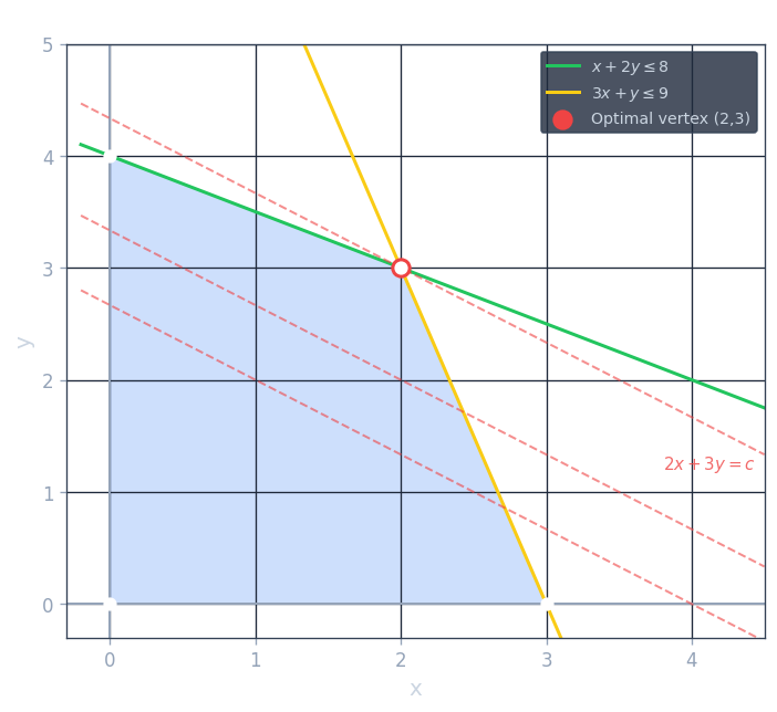
The key geometric observation is that the optimal point, if it exists, can always be taken to be a vertex of the polytope — a corner point where the polytope cannot be expressed as the midpoint of two other feasible points. Intuitively, if we slide along the direction \( c \) until we hit the boundary, we will eventually reach a corner. If the corner is integral, we are done. If we can show that all corners of the LP relaxation are integral, then the LP automatically solves the ILP.

This geometric intuition motivates a precise algebraic definition. For the inequality form LP, we say that a constraint \( A_i x \leq b_i \) is tight at a point \( x \) if equality holds: \( A_i x = b_i \). Let \( A^= \) denote the submatrix of tight constraints. We call \( x \) a basic feasible solution (BFS) if (a) \( x \) is feasible, and (b) the matrix \( A^= \) of tight constraints has rank \( n \) — in other words, the tight constraints uniquely determine \( x \).

There are three equivalent characterizations of corner points:

1. Vertex solution: \( x \in P \) such that there is no direction \( y \neq 0 \) with both \( x + y \in P \) and \( x - y \in P \). Geometrically, \( x \) is not the midpoint of two other feasible points.
2. Extreme point solution: \( x \in P \) is the unique optimal solution for some objective vector \( c \).
3. Basic feasible solution: \( x \in P \) satisfies rank\( (A^=) = n \).

Proposition. These three definitions are equivalent.

The equivalence \( 3 \Rightarrow 2 \) is proved as follows. If \( x \) is a BFS with support \( S = \{j \mid x_j > 0\} \), we can choose an objective function \( c \) with \( c_j = 0 \) for \( j \in S \) and \( c_j = 1 \) for \( j \notin S \). Then \( x \) achieves objective value 0, and any other solution \( y \) with objective value 0 must have \( y_j = 0 \) for \( j \notin S \). The tight constraints for \( x \) uniquely determine a solution with this support, so \( y = x \). Thus \( x \) is the unique optimal solution.

The direction \( 1 \Rightarrow 3 \) is proved by contrapositive. If the tight constraints do not have full rank, there exists \( y \neq 0 \) with \( A^= y = 0 \) and \( \text{supp}(y) \subseteq \text{supp}(x) \). For small enough \( \varepsilon > 0 \), both \( x + \varepsilon y \) and \( x - \varepsilon y \) remain feasible (the tight constraints remain satisfied as equalities, and the strict inequalities remain strict), so \( x \) is not a vertex.

Theorem (Existence of optimal BFS). For any bounded polytope \( P \) and any objective \( c \), there exists a basic feasible solution \( x^* \) that is optimal.

The proof constructs an optimal BFS by starting from any optimal solution and moving along the tight constraint space to acquire more tight constraints. If the current point is not a BFS, there exists a direction \( y \neq 0 \) with \( A^= y = 0 \). Moving in direction \( y \) does not loosen any tight constraint; it maintains feasibility until it hits a new constraint, gaining one more tight constraint while not increasing (or perhaps decreasing) the objective. Since there are finitely many constraints, this process terminates at a BFS. Crucially, the objective value does not increase along the way, so the final BFS is still optimal.

This theorem is the foundation of the LP approach to combinatorial optimization: if we can show every BFS is integral, then solving the LP gives an integral optimal solution.

16.4 Basic Feasible Solutions and Integrality

To show that the LP relaxation of a specific combinatorial problem is tight, we need to show that every BFS of the polytope is integral. The standard approach is the rank argument, illustrated here for the perfect bipartite matching LP.

Consider the LP: maximize \( \sum_e w_e x_e \) subject to \( \sum_{e \in \delta(v)} x_e = 1 \) for all \( v \in V \) (every vertex is matched exactly once), and \( 0 \leq x_e \leq 1 \) for all \( e \). Suppose \( x \) is a BFS with \( 0 < x_e < 1 \) for some edge \( e = uv \). Since the degree constraint at \( u \) requires \( \sum_{e \in \delta(u)} x_e = 1 \) and no edge is fully saturated, there must be another edge incident to \( u \) with \( 0 < x < 1 \). Following this chain of fractional edges, we eventually find a cycle. Since the graph is bipartite, this cycle is even. Along this even cycle, we can define a perturbation \( y \) by alternately adding and subtracting \( \varepsilon \) around the cycle, producing two distinct feasible solutions \( x + \varepsilon y \) and \( x - \varepsilon y \). This contradicts the fact that \( x \) is a vertex.

Therefore, every BFS of the bipartite matching LP is integral, and we can solve the matching problem by solving the LP. We will revisit this argument more carefully in Chapter 17 via the rank method.

16.5 Algorithms for Linear Programming

There are three main families of algorithms for solving LPs in practice and theory.

The simplex method. Devised by Dantzig in 1947, the simplex method works in the standard form. It starts at a BFS and repeatedly moves to an adjacent BFS — one obtained by swapping one variable entering the support and one variable leaving it — as long as the objective improves. When no improving neighbor exists, the current solution is optimal (since a locally optimal point of a convex problem is globally optimal).

The simplex method is remarkably practical. On real-world problems, it typically terminates in \( O(m) \) or \( O(n) \) pivots, which is much less than the exponential worst case. In 1972, Klee and Minty constructed an LP in \( n \) variables where the simplex method with the natural “steepest ascent” pivot rule visits all \( 2^n \) vertices before finding the optimum. It remains an open problem whether there exists a pivot rule that makes the simplex method polynomial. A related open problem is whether every polytope has a diameter at most polynomial in \( n \) and \( m \) (the Hirsch conjecture, which was disproved for the general case in 2010 but remains open for LP polytopes).

An important observation is that many combinatorial algorithms can be interpreted as the simplex method with a specific pivot rule. The augmenting path algorithm for matching, for example, corresponds to pivoting in the matching LP. This provides a unified perspective on seemingly different algorithms.

The ellipsoid method. Khachiyan’s 1979 algorithm was the first to prove that LP can be solved in polynomial time. The key idea is to reduce LP optimization to LP feasibility (checking whether a system has a feasible point), and to solve feasibility by maintaining an ellipsoid guaranteed to contain the feasible set. At each step, we check whether the center of the current ellipsoid is feasible. If yes, we are done. If not, we invoke a separation oracle to find a hyperplane separating the center from the feasible region. The algorithm then computes the minimum-volume ellipsoid containing the half of the current ellipsoid on the feasible side. One can show that each step reduces the volume by a factor of \( e^{-1/(2(n+1))} \), so after \( O(n) \) steps the volume becomes negligibly small, proving that the feasible set must be empty.

The most significant feature of the ellipsoid method is that it only requires a separation oracle — an algorithm that, given a point \( x \), either certifies that \( x \) is feasible or returns a constraint violated by \( x \). This means we do not need to write down all constraints explicitly. If there is a polynomial-time separation oracle for an exponentially large LP, the ellipsoid method solves it in polynomial time. The spanning tree LP, with exponentially many subtour elimination constraints, is one such example: the minimum-cut computation acts as the separation oracle. We will see this in detail in Chapter 18.

The deep theorem underlying this approach is:

Theorem (Optimization ≡ Separation). A polynomial-time algorithm for LP optimization exists if and only if a polynomial-time separation oracle exists. More precisely, given a family of polytopes described implicitly, LP optimization over these polytopes is polynomial-time equivalent to the separation problem.

Interior point methods. Karmarkar’s 1984 algorithm was the first polynomial-time method that is also competitive with simplex in practice. Rather than moving along the boundary of the polytope, interior point methods begin at a strictly feasible interior point and move through the interior, guided by “barrier functions” that steer the trajectory away from the boundary. The logarithmic barrier \( -\sum_i \log(b_i - A_i x) \) penalizes proximity to constraint boundaries, ensuring iterates stay feasible. Newton’s method is applied to a sequence of increasingly weakly penalized subproblems, each approximated as an unconstrained quadratic program, and the solution converges to the LP optimum. Modern interior point algorithms run in \( O((m + n)^{1.5} n^{0.5} \cdot L) \) arithmetic operations where \( L \) is the input bit length, and in practice they are highly competitive with simplex.

16.6 Integer LP: The Hard Part

Adding integrality constraints \( x_i \in \{0, 1\} \) to an LP generally makes the problem NP-hard. The LP relaxation serves as the primary tool for studying ILPs:

• It provides a lower bound on the optimum (for minimization) or an upper bound (for maximization).
• It can be used to design approximation algorithms by rounding the fractional LP solution to an integral solution in a controlled way.
• For special problem classes, the LP relaxation itself has only integral extreme points, making it an exact solver.

The study of when LP relaxations are integral — and how much information they lose when they are not — is the unifying theme of the next three chapters.

Section 3.2: Matching Polytopes

17.1 Setting Up the LP

The maximum bipartite matching problem is one of the central problems in combinatorial optimization: given a bipartite graph \( G = (A \cup B, E) \) with edge weights \( w_e \geq 0 \), find a maximum-weight subset of edges such that every vertex is incident to at most one chosen edge.

The natural LP relaxation assigns a variable \( x_e \in [0, 1] \) to each edge \( e \), with the constraint that the total fractional matching at each vertex is at most 1:

This LP is a relaxation: any integer matching \( x \in \{0,1\}^E \) satisfying the degree constraints is feasible. We want to show the LP always has an integral optimal solution.

17.2 The Rank Argument

The proof proceeds by induction on the number of edges. We will show that in any basic feasible solution \( x \), there must exist an edge \( e \) with \( x_e \in \{0, 1\} \). Given such an edge:

• If \( x_e = 0 \): delete edge \( e \). The LP on the smaller graph has the same optimal value, and by induction has an integral optimal solution.
• If \( x_e = 1 \): include \( e = uv \) in the matching, remove vertices \( u \) and \( v \) and all their incident edges. The remaining LP solution (restricted to the smaller graph) is feasible with value \( \text{opt}(G) - w_e \). By induction, the smaller LP has an integral solution of value \( \text{opt}(G) - w_e \), and adding edge \( e \) gives an integral solution of value \( \text{opt}(G) \).

Lemma. In any basic feasible solution of the bipartite matching LP, there exists an edge \( e \) with \( x_e \in \{0, 1\} \).

Proof. Suppose for contradiction that \( 0 < x_e < 1 \) for all \( e \in E \). Since \( x_e > 0 \) for all edges, the only tight constraints are degree constraints. Let \( W \) be the set of vertices \( v \) with \( \sum_{e \in \delta(v)} x_e = 1 \) (tight degree constraint).

In any BFS, the number of tight linearly independent constraints equals the number of variables, which is \( |E| \). Therefore \( |W| \geq |E| \).

Since every \( x_e < 1 \) and every vertex in \( W \) has tight degree constraint \( \sum_e x_e = 1 \), every vertex in \( W \) must have degree at least 2 (you cannot reach a total of 1 using one edge with \( x_e < 1 \)). Vertices not in \( W \) contribute no tight constraints, so they have degree 0 (otherwise \( x_e > 0 \) would force a tight constraint). Summing degrees:

So all inequalities are equalities: \( \deg(v) = 2 \) for \( v \in W \) and \( \deg(v) = 0 \) for \( v \notin W \). This means the graph induced on \( W \) is a disjoint union of cycles.

Now we show the tight constraints are linearly dependent. Let \( W_1 \) and \( W_2 \) be the two sides of the bipartite graph restricted to \( W \) (well-defined since the graph is bipartite). Each edge \( e \) is incident to exactly one vertex in \( W_1 \) and one in \( W_2 \). The vector \( \sum_{v \in W_1} \chi_{\delta(v)} \) assigns to each edge a value equal to the number of \( W_1 \)-endpoints it has. Since every edge in \( E \) has exactly one endpoint in \( W_1 \) (as vertices outside \( W \) have degree 0), this sum equals \( \chi_E \). Similarly \( \sum_{v \in W_2} \chi_{\delta(v)} = \chi_E \). Therefore \( \sum_{v \in W_1} \chi_{\delta(v)} = \sum_{v \in W_2} \chi_{\delta(v)} \), which shows the tight constraints are linearly dependent. The rank of the tight constraints is at most \( |W| - 1 = |E| - 1 \), contradicting the assumption that \( x \) is a basic solution with \( |E| \) linearly independent tight constraints. \( \square \)

Corollary (Integrality of bipartite matching LP). Every extreme point of the bipartite matching LP polytope is integral.

This means solving the LP gives a maximum-weight matching directly, without any rounding step.

17.3 Total Unimodularity

The integrality of the bipartite matching LP is a consequence of a deeper structural property: the constraint matrix is totally unimodular (TU). A matrix \( A \) is TU if every square submatrix has determinant 0, \( +1 \), or \( -1 \).

Theorem. The vertex-edge incidence matrix of a bipartite graph is totally unimodular.

The proof follows from the Ghouila-Houri characterization: a \( \{0, \pm 1\} \) matrix \( A \) is TU if and only if every subset of rows can be partitioned into two classes \( R^+, R^- \) such that for every column \( j \), \( |\sum_{i \in R^+} A_{ij} - \sum_{i \in R^-} A_{ij}| \leq 1 \). For the bipartite incidence matrix (where each column has exactly two 1’s, one in each side of the bipartition), we assign \( R^+ = A \) (one side) and \( R^- = B \) (other side). Each column \( e = (a, b) \) contributes \( +1 \) from the \( R^+ \) side and \( +1 \) from the \( R^- \) side, giving \( |1 - 1| = 0 \leq 1 \). So the matrix is TU.

Why does TU imply integrality? When \( A \) is TU and \( b \) is an integer vector, every basic feasible solution of \( Ax \leq b \), \( x \geq 0 \) is integral. The reason: a BFS is determined by \( n \) linearly independent tight constraints, so \( x = (A^=)^{-1} b^= \) where \( A^= \) is an \( n \times n \) submatrix of \( A \) (plus identity rows from \( x \geq 0 \)). By Cramer’s rule, each coordinate \( x_j = \det(M_j) / \det(A^=) \) where \( M_j \) is \( A^= \) with one column replaced by \( b^= \). Since \( A \) is TU, all these determinants are \( 0 \) or \( \pm 1 \), so \( x_j \) is always an integer.

17.4 König’s Theorem via LP Duality

One of the most elegant consequences of LP integrality is König’s theorem:

Theorem (König, 1916). In any bipartite graph, the maximum size of a matching equals the minimum size of a vertex cover.

This follows immediately from LP duality. The dual of the bipartite matching LP is:

An integer solution to the dual is a vertex cover: we include vertex \( v \) in the cover if \( y_v = 1 \). The LP duality theorem tells us that the primal and dual optima are equal, and since both LPs are integral (the primal by TU, the dual also by TU of the transpose), the integral optima are equal: maximum matching equals minimum vertex cover.

This argument beautifully illustrates the LP perspective on classical combinatorial theorems: they are nothing but duality statements for integral LPs.

17.5 Non-Bipartite Matching and Edmonds’ Polytope

The bipartite matching LP is not integral for general graphs. Consider a triangle \( K_3 \): set \( x_e = 1/2 \) for all three edges. This satisfies all degree constraints (each vertex has total \( 1 = 1/2 + 1/2 \)) and achieves objective value \( 3/2 \), but the maximum integral matching has value 1. The LP integrality fails because odd cycles allow “fractional” half-integral solutions.

To obtain an integral LP for general matching, Edmonds (1965) added the odd-set constraints:

Here \( E(S) \) denotes the set of edges with both endpoints in \( S \). An odd set cannot contain more than \( \lfloor |S|/2 \rfloor \) edges in a matching, so any integral solution satisfies these constraints. Edmonds famously proved that this exponential-size LP is integral — every extreme point is a \( \{0,1\} \) vector — and that a polynomial-time separation oracle exists (solvable via minimum odd cut). Thus matching in general graphs can be solved in polynomial time via this LP.

Rothvoss (2014) proved a striking lower bound: any LP formulation of the matching polytope requires exponentially many constraints. There is no polynomial-size LP whose feasible region is exactly the matching polytope of a general graph. This shows that the exponential size of Edmonds’ LP is in some sense necessary.

17.6 Extension: The 3-Dimensional Matching Approximation

The rank argument extends to NP-hard problems to give approximation algorithms. In the 3-dimensional matching problem, we have three sets \( X, Y, Z \) of size \( n \) and a collection of triples \( (x_i, y_j, z_k) \). The goal is to find the maximum collection of disjoint triples. The natural LP relaxation has degree constraints \( \sum_{e \ni v} x_e \leq 1 \) for all \( v \).

A rank argument analogous to the bipartite case shows that in any BFS, there must exist a hyperedge \( e \) with \( x_e \geq 1/2 \). The key step: if all \( x_e < 1/2 \), every vertex in the tight set has degree at least 3. Summing degrees gives \( |W| \geq |E| = \frac{1}{3} \sum \deg \geq |W| \), with equality forcing degree exactly 3 and a linear dependence among the tight constraints (using the tripartition into \( W_X, W_Y, W_Z \)). Finding a hyperedge with \( x_e \geq 1/2 \) and adding it to the solution, then removing at most \( 3 \cdot (1 - x_e) \leq 3(1 - 1/2) = 3/2 \) fractional units of the remaining LP, gives a \( 1/2 \)-approximation by induction.

Section 3.3: Spanning Tree Polytopes

18.1 The Subtour Elimination LP

The minimum spanning tree problem can be formulated as the following LP:

Here \( E(S) \) denotes the set of edges with both endpoints in \( S \), and \( x(E(S)) = \sum_{e \in E(S)} x_e \). The constraint \( x(E(S)) \leq |S| - 1 \) forbids cycles: any spanning subgraph of \( S \) with at least \( |S| \) edges must contain a cycle. The equality constraint \( x(E(V)) = |V| - 1 \) requires exactly \( n - 1 \) edges in total. Together, these constraints force any integral solution to be a spanning tree.

This LP has exponentially many constraints — one for each non-empty proper subset \( S \subsetneq V \), giving \( 2^n - 2 \) constraints. Despite this, the LP can be solved in polynomial time via the ellipsoid method, provided we have a polynomial-time separation oracle.

18.2 The Separation Oracle

Given a vector \( x \in \mathbb{R}^E \), the separation oracle must either certify that \( x \) satisfies all subtour elimination constraints, or exhibit a violating set \( S \). The constraint \( x(E(V)) = n - 1 \) is easy to check directly. For the subtour elimination constraints, the following min-cut reduction works.

For each vertex \( v_i \), construct a directed network as follows: create one source node \( s \), one node per edge \( e_j \), and one node per vertex of the original graph. Add an arc from \( s \) to edge-node \( e_j \) with capacity \( x_{e_j} \). For each edge \( e_j = (u, v) \), add arcs from \( e_j \)-node to \( u \)-node and to \( v \)-node, each with capacity \( \infty \). For each vertex \( v_j \neq v_i \), add an arc from \( v_j \)-node to a sink \( t \) with capacity 1. The special vertex \( v_i \) has no arc to \( t \).

Lemma. There is a violating set containing \( v_i \) if and only if the minimum \( s \)-\( t \) cut value is strictly less than \( |V| - 1 \).

The intuition: if a set \( S \ni v_i \) satisfies \( x(E(S)) > |S| - 1 \), then the total capacity entering the \( S \)-vertices from edge-nodes is \( x(E(S)) \), but only \( |S| - 1 \) units can exit to \( t \) (since \( v_i \) has no exit), so the max-flow is less than \( |V| - 1 \), meaning the min-cut is also less. The formal proof traces the cut structure.

Running this construction for each vertex \( v_i \) takes \( O(n) \) max-flow computations. If all min-cuts equal \( n-1 \), the solution is feasible; otherwise, the cut reveals a violated constraint. This gives a polynomial-time separation oracle, so the ellipsoid method solves the spanning tree LP in polynomial time.

18.3 Integrality via the Uncrossing Technique

Theorem. Every basic optimal solution of the subtour elimination LP is a \( \{0,1\} \) vector corresponding to a spanning tree.

The proof has two parts. First, we show the number of linearly independent tight constraints is at most \( n - 1 \). Then we use this to conclude that any BFS has at most \( n - 1 \) non-zero variables, each equal to 1.

Call a set \( S \subseteq V \) tight if \( x(E(S)) = |S| - 1 \). Let \( \mathcal{F} \) be the family of all tight sets. The key observation is an algebraic identity for the characteristic vectors \( \chi_{E(S)} \in \mathbb{R}^E \) (the indicator vectors of edge sets):

Claim. For any \( S, T \subseteq V \), we have \( \chi_{E(S)} + \chi_{E(T)} \leq \chi_{E(S \cap T)} + \chi_{E(S \cup T)} \), with equality if and only if there are no edges with one endpoint in \( S \setminus T \) and the other in \( T \setminus S \).

This follows by case analysis on how each edge \( e \) contributes to both sides:

• If both endpoints are in \( S \cap T \): contributes 1 to \( E(S) \), 1 to \( E(T) \), 1 to \( E(S \cap T) \), 1 to \( E(S \cup T) \) — both sides get 2.
• If one endpoint is in \( S \setminus T \) and both are in \( S \cup T \): contributes 1 to \( E(S) \), 0 to \( E(T) \), 0 to \( E(S \cap T) \), 1 to \( E(S \cup T) \) — both sides get 1 (or 0 on the RHS if the second endpoint is in \( T \setminus S \), making it a “dotted” edge that contributes 0 on the LHS but 1 on the RHS).

Lemma (Uncrossing). If \( S, T \in \mathcal{F} \) and \( S \cap T \neq \emptyset \), then both \( S \cap T \) and \( S \cup T \) are in \( \mathcal{F} \), and \( \chi_{E(S)} + \chi_{E(T)} = \chi_{E(S \cap T)} + \chi_{E(S \cup T)} \).

All inequalities are equalities. The second equality forces both \( S \cap T \) and \( S \cup T \) to be tight; the first equality forces the linear relation \( \chi_{E(S)} + \chi_{E(T)} = \chi_{E(S \cap T)} + \chi_{E(S \cup T)} \). \( \square \)

The linear relation means that whenever two sets \( S, T \in \mathcal{F} \) intersect, their characteristic vectors satisfy a dependency: \( \chi_{E(S)} + \chi_{E(T)} = \chi_{E(S \cap T)} + \chi_{E(S \cup T)} \). This is the uncrossing lemma — the two intersecting sets can be replaced by their intersection and union without losing span.

Theorem. The number of linearly independent subtour elimination constraints is at most \( |V| - 1 \).

Proof. We claim that there exists a laminar family \( \mathcal{L} \subseteq \mathcal{F} \) such that \( \text{span}(\mathcal{L}) = \text{span}(\mathcal{F}) \), where a laminar family is a family with no two intersecting sets — every pair satisfies \( S \subseteq T \) or \( T \subseteq S \) or \( S \cap T = \emptyset \).

Take a maximal laminar subfamily \( \mathcal{L} \subseteq \mathcal{F} \). We claim \( \text{span}(\mathcal{L}) = \text{span}(\mathcal{F}) \). Suppose for contradiction that some \( R \in \mathcal{F} \) is not in \( \text{span}(\mathcal{L}) \); choose such \( R \) minimizing the number of sets in \( \mathcal{L} \) that intersect \( R \). Since \( \mathcal{L} \) is maximal laminar, some \( S \in \mathcal{L} \) intersects \( R \). By the uncrossing lemma, both \( S \cap R \) and \( S \cup R \) are in \( \mathcal{F} \), and \( \chi_{E(S)} + \chi_{E(R)} = \chi_{E(S \cap R)} + \chi_{E(S \cup R)} \).

We verify that both \( S \cap R \) and \( S \cup R \) intersect strictly fewer sets in \( \mathcal{L} \) than \( R \) does. For any \( T \in \mathcal{L} \) with \( T \neq S \): since \( T \) and \( S \) do not intersect (both are in \( \mathcal{L} \)), \( T \) intersects \( S \cap R \) or \( S \cup R \) only if it intersects \( R \). But \( S \) itself intersects \( R \) but not \( S \cap R \) or \( S \cup R \) (well, it contains \( S \cap R \) and is contained in \( S \cup R \), so it does not intersect them in the strict sense). So the number of intersectors strictly decreases.

By the minimality of \( R \), both \( S \cap R \) and \( S \cup R \) are in \( \text{span}(\mathcal{L}) \). Since \( S \in \mathcal{L} \subseteq \text{span}(\mathcal{L}) \), the identity \( \chi_{E(R)} = \chi_{E(S \cap R)} + \chi_{E(S \cup R)} - \chi_{E(S)} \) puts \( R \) in \( \text{span}(\mathcal{L}) \), a contradiction. \( \square \)

A laminar family on a ground set of \( n \) elements with no singletons has at most \( n - 1 \) members (provable by induction on the tree structure). Since the subtour constraints have no singleton tight sets (a single vertex \( v \) gives \( x(E(\{v\})) = 0 = 1 - 1 \), which is vacuously tight but empty), the laminar family \( \mathcal{L} \) has at most \( n - 1 \) sets. Therefore, the rank of the tight constraints is at most \( n - 1 \).

Completing the integrality proof. Let \( x \) be a basic optimal solution. Remove all edges with \( x_e = 0 \). The number of non-zero variables equals at most the rank of the tight constraint system, which is at most \( n - 1 \). Note that \( x_e \leq 1 \) for all \( e \), since the constraint \( x(E(\{u,v\})) \leq 1 \) is a tight subtour constraint for the two-element set \( \{u, v\} \). Now, \( x(E(V)) = n - 1 \) with at most \( n - 1 \) non-zero variables each at most 1 forces each non-zero \( x_e = 1 \). The resulting solution is a spanning tree. \( \square \)

18.4 Bounded-Degree Spanning Trees

Theorem (Singh-Lau, 2007). If there is a spanning tree with cost \( C \) satisfying \( \deg(v) \leq B_v \) for all \( v \), there is a polynomial-time algorithm that finds a spanning tree with cost at most \( C \) and \( \deg(v) \leq B_v + 2 \) for all \( v \).

This is a striking result: for an NP-hard problem (when degree bounds are required to be exact), we can satisfy all bounds up to an additive +2 violation with no cost increase.

The algorithm uses the LP relaxation augmented with degree constraints \( x(\delta(v)) \leq B_v \) for all \( v \in W \) (the set of degree-constrained vertices):

The iterative rounding algorithm works as follows:

1. Compute a basic optimal solution. Remove all edges with \( x_e = 0 \).
2. If some vertex \( u \) has only one incident edge \( uv \) with \( x_{uv} > 0 \), then \( x_{uv} = 1 \) (by the spanning tree constraints). Add \( uv \) to the solution, contract \( v \) into the tree, update \( B_u \leftarrow B_u - 1 \).
3. If some vertex \( v \) has degree at most 3 (counting edges with \( x_e > 0 \)), remove the degree constraint on \( v \).
4. Return to step 1.

Analysis. Step 2 only adds edges with \( x_e = 1 \), so the cost is at most the LP optimum. For degree violations: when we remove the constraint on \( v \) in step 3, at most 3 edges are incident to \( v \) with positive \( x_e \). In the worst case, all 3 are added to the tree, and we have \( \deg(v) \leq B_v + 2 \) (since we already count some of those edges in the fractional solution).

Why does the algorithm always terminate? The key claim is that in every basic solution of this LP, at least one of the following holds: some \( x_e = 0 \), some vertex has degree 1, or some degree-constrained vertex has degree at most 3. The proof is by counting: suppose none of these hold. Then \( \deg(v) \geq 4 \) for \( v \in W \) and \( \deg(v) \geq 2 \) for \( v \notin W \). This gives \( |E| \geq \frac{1}{2}(4|W| + 2(|V|-|W|)) = |V| + |W| \). But the number of linearly independent tight constraints is at most \( (|V| - 1) + |W| \) (at most \( n - 1 \) tight subtour constraints plus at most \( |W| \) tight degree constraints). So the rank is at most \( |V| + |W| - 1 < |E| \), contradicting the assumption that \( x \) is a basic solution.

This counting argument is the signature of the iterative rounding technique: a dimension argument forces progress at every step of the algorithm.

Section 3.4: LP Duality

19.1 The Dual Program

LP duality is one of the deepest ideas in optimization. It says that every maximization LP has a corresponding minimization LP — its dual — and the two programs have the same optimal value. More than an abstract theorem, duality is a practical tool: the dual program gives a certificate of optimality, connects LP to combinatorial min-max theorems, and underlies important classes of algorithms.

Every dual-feasible \( y \) gives an upper bound \( \langle b, y \rangle \) on the primal optimal, and the dual asks for the tightest such bound.

The symmetry of duality is remarkable: the dual of the dual is the primal. If you form the dual of program (D), you recover (P).

19.2 Weak Duality

Proof. \( \langle c, x \rangle \leq \langle A^T y, x \rangle = y^T (Ax) \leq y^T b = \langle b, y \rangle \), where the first inequality uses \( A^T y \geq c \) and \( x \geq 0 \), and the second uses \( Ax \leq b \) and \( y \geq 0 \). \( \square \)

Weak duality immediately gives: any feasible dual solution \( y \) provides an upper bound \( \langle b, y \rangle \) on the primal optimum. This is extremely useful: to prove a primal solution \( x^* \) is optimal, exhibit a dual solution \( y^* \) with \( \langle c, x^* \rangle = \langle b, y^* \rangle \).

19.3 Complementary Slackness

The conditions for a primal-dual pair to be simultaneously optimal are elegant:

Theorem (Complementary Slackness). Primal-feasible \( x \) and dual-feasible \( y \) are both optimal if and only if:

1. (Primal CS): \( x_j > 0 \Rightarrow (A^T y)_j = c_j \) (the \( j \)-th dual constraint is tight), and
2. (Dual CS): \( y_i > 0 \Rightarrow (Ax)_i = b_i \) (the \( i \)-th primal constraint is tight).

In words: a primal variable can be positive only if the corresponding dual constraint is met with equality, and a dual variable can be positive only if the corresponding primal constraint is met with equality.

Proof. From the proof of weak duality, \( \langle b, y \rangle - \langle c, x \rangle = (y^T b - y^T A x) + (y^T A x - c^T x) = y^T(b - Ax) + (A^T y - c)^T x \). Both terms are non-negative (since \( y, b - Ax, A^T y - c, x \geq 0 \)). Their sum is zero if and only if both are zero: \( y^T(b - Ax) = 0 \) means \( y_i(b_i - (Ax)_i) = 0 \) for all \( i \) (dual CS), and \( (A^T y - c)^T x = 0 \) means \( ((A^T y)_j - c_j) x_j = 0 \) for all \( j \) (primal CS). \( \square \)

Complementary slackness conditions are the foundation of primal-dual algorithms: start with a dual-feasible solution, adjust the primal to improve primal feasibility while maintaining complementary slackness, and update the dual accordingly. This approach gives efficient combinatorial algorithms for matching (the Hungarian algorithm), shortest paths (Dijkstra’s algorithm), and network flow.

19.4 Strong Duality

The proof uses the Farkas lemma and the separation theorem from convex analysis.

Theorem (Farkas’ Lemma). The system \( Ax = b \), \( x \geq 0 \) is infeasible if and only if there exists \( y \) such that \( y^T A \geq 0 \) and \( y^T b < 0 \).

In other words, either the system has a solution, or there is a certificate of infeasibility. This is a theorem of alternatives: exactly one of the two alternatives holds. The proof uses the separation theorem: the set \( S = \{Ax \mid x \geq 0\} \) is a closed convex cone. If \( b \notin S \), the hyperplane separation theorem gives a \( y \) with \( y^T b < y^T z \) for all \( z \in S \); since \( 0 \in S \), we get \( y^T b < 0 \), and since \( S \) contains all \( Ax \) for \( x \geq 0 \), we get \( y^T A \geq 0 \).

Proof of strong duality. Let \( \mu \) be the primal optimal value. We want a dual solution with objective value \( \mu \). The primal optimum being less than any \( \mu' > \mu \) means the system \( c^T x \geq \mu', Ax = b, x \geq 0 \) is infeasible. By Farkas’ lemma (in a slightly extended form), this infeasibility implies the existence of \( y \in \mathbb{R}^m \) and \( z \leq 0 \) such that \( y^T A + z c^T \geq 0 \), \( -z \geq 0 \), and \( y^T b + z \mu' < 0 \). If \( z \neq 0 \) (so \( z < 0 \)), dividing by \( -z \) gives a dual feasible solution \( y' = y/(-z) \) with \( (y')^T b < \mu' \). As \( \mu' \to \mu \), this yields a dual solution achieving value \( \mu \). \( \square \)

19.5 Applications of Duality

Max-flow min-cut. The LP formulation of maximum flow has a dual that corresponds precisely to minimum \( s \)-\( t \) cuts. The primal assigns flow variables to each directed edge; the dual assigns potential variables to each vertex. A dual solution with \( y_s = 1 \), \( y_t = 0 \), \( y_v \in [0,1] \) corresponds to a fractional cut, and integrality of both programs (provable by TU arguments) gives the integer max-flow min-cut theorem.

König’s theorem. As seen in Chapter 17, the bipartite matching LP and its dual (vertex cover LP) are both integral, and strong duality gives König’s theorem: maximum matching equals minimum vertex cover.

The minimax theorem (von Neumann, 1928). In a two-player zero-sum game with payoff matrix \( A \in \mathbb{R}^{m \times n} \), the row player maximizes expected payoff by choosing a mixed strategy \( x \in \Delta^m \) (a probability distribution over rows), and the column player minimizes by choosing \( y \in \Delta^n \). The minimax theorem states:

The left side is the maximin: the row player announces first (gains from commitment). The right side is the minimax: the column player announces first. The equality says there is no advantage to moving first — there is a saddle point.

These two LPs are duals of each other, so strong duality gives the minimax theorem.

To lower-bound the complexity of any randomized algorithm, it suffices to exhibit an input distribution under which every deterministic algorithm is slow. This technique is widely used in complexity theory.

Section 3.5: The Multiplicative Weight Update Method

20.1 The Online Experts Problem

Imagine you are managing a portfolio and consult \( n \) financial advisors (experts) over \( T \) time periods. Each day, you choose how to distribute your investments among the \( n \) options, and at the end of each day you learn how each option performed. Can you guarantee performance close to the best single advisor in hindsight — even without knowing in advance who the best advisor will be?

Surprisingly, yes. The multiplicative weight update (MWU) method provides a simple algorithm with a provably small regret — the difference between our cumulative loss and the loss of the best single expert.

More formally: there are \( n \) experts and \( T \) rounds. In round \( t \), we choose a probability distribution \( p^{(t)} \in \Delta^n \) over the experts (representing how we blend their advice), and then observe the loss vector \( m^{(t)} \in [-1, +1]^n \), where \( m_i^{(t)} \) is the loss of expert \( i \) in round \( t \). Our cost in round \( t \) is \( \langle m^{(t)}, p^{(t)} \rangle \). The goal is to minimize total cost \( \sum_{t=1}^T \langle m^{(t)}, p^{(t)} \rangle \) relative to the best expert.

Note that the loss vector can be chosen adversarially — nature (or an adversary) can set \( m^{(t)} \) after seeing our distribution \( p^{(t)} \). Even in this worst case, MWU gives a useful guarantee.

20.2 The Algorithm

Fix a learning rate parameter \( \eta \leq 1/2 \). Initialize weights \( w_i^{(1)} = 1 \) for all \( 1 \leq i \leq n \).

For each round \( t = 1, \ldots, T \):

1. Let \( \Phi^{(t)} = \sum_{i=1}^n w_i^{(t)} \) be the total weight. Set \( p_i^{(t)} = w_i^{(t)} / \Phi^{(t)} \).
2. Observe the loss vector \( m^{(t)} \).
3. Update weights: \( w_i^{(t+1)} = w_i^{(t)} \cdot (1 - \eta m_i^{(t)}) \).

The weight update multiplicatively increases the weight of experts with negative loss (they did well) and decreases the weight of experts with positive loss (they did poorly). Since \( m_i^{(t)} \in [-1, +1] \) and \( \eta \leq 1/2 \), the update factor \( 1 - \eta m_i^{(t)} \) is always positive.

20.3 The Regret Bound

Setting \( \eta = \sqrt{(\ln n) / T} \) (assuming all losses in \( [0,1] \)) gives regret at most \( 2\sqrt{T \ln n} \) — sublinear in \( T \), meaning the average regret per round vanishes.

Proof. Use \( \Phi^{(t)} = \sum_i w_i^{(t)} \) as a potential function.

Rearranging gives the claimed bound. \( \square \)

20.4 Applying MWU to Solve Linear Programs

The MWU framework gives an elegant, general method for approximately solving LPs. Consider the feasibility problem \( Ax \geq b \), \( x \geq 0 \), where \( A \in \mathbb{R}^{m \times n} \). We call the constraints \( x \geq 0 \) the “easy” constraints and the \( m \) constraints \( A_i x \geq b_i \) the “hard” constraints.

The reduction. Think of each constraint \( A_i x \geq b_i \) as an “expert.” If the oracle proposes a solution \( x^{(t)} \) that violates constraint \( i \), that constraint is “happy” (its violation is the oracle’s loss). The MWU method combines the constraints into a single weighted constraint \( \langle p^{(t)}, Ax \rangle \geq \langle p^{(t)}, b \rangle \) (where \( p^{(t)} \) is the current weight distribution). An oracle solves this single constraint along with the easy constraints.

Algorithm. Initialize \( p^{(1)} = \mathbf{1}/m \). For \( t = 1, \ldots, T \):

1. Use the oracle to find \( x^{(t)} \) satisfying \( p^{(t)} A x \geq p^{(t)} b \) and \( x \geq 0 \), with the guarantee that \( |A_i x^{(t)} - b_i| \leq w \) for all \( i \) (bounded width \( w \)).
2. Set \( m_i^{(t)} = (A_i x^{(t)} - b_i)/w \in [-1, +1] \).
3. Update weights multiplicatively.

Return \( \bar{x} = \frac{1}{T} \sum_{t=1}^T x^{(t)} \).

Theorem. With width \( w \) and \( T = 4w^2 \ln m / \varepsilon^2 \) rounds, the returned solution \( \bar{x} \) satisfies \( A_i \bar{x} \geq b_i - \varepsilon \) for all \( i \).

Setting \( \eta = \varepsilon / (2w) \) and \( T = 4w^2 \ln m / \varepsilon^2 \), the right side rearranges to \( \sum_t m_i^{(t)} \geq -\varepsilon T / w \), meaning \( A_i \bar{x} \geq b_i - \varepsilon \). \( \square \)

The key quantity is the width \( w \): the maximum violation \( |A_i x^{(t)} - b_i| \). Smaller width means fewer oracle calls and a faster algorithm. The width is determined by the structure of the oracle — a crucial design choice.

For LPs arising from combinatorial problems, a straightforward oracle gives width \( w = O(n) \), leading to \( O(n^2 \ln m / \varepsilon^2) \) iterations. For maximum flow, the electrical flow oracle achieves width \( w = O(\sqrt{m}) \), giving \( O(\sqrt{m} \ln m / \varepsilon^2) \) iterations — a significant improvement that we explore in the next chapter.

20.5 Connection to Game Theory and the Minimax Theorem

The MWU framework provides an algorithmic proof of the minimax theorem. In a two-player zero-sum game with payoff matrix \( A \), run MWU as the row player’s strategy and play a best-response (minimum payoff column) each round. The average play of each player converges to a Nash equilibrium. By the MWU regret bound, the row player achieves average payoff at least \( \text{OPT} - O(\sqrt{(\ln n)/T}) \), where \( \text{OPT} \) is the minimax value. This gives an algorithmic construction of equilibria convergent in \( O((\ln n)/\varepsilon^2) \) rounds.

Section 3.6: Maximum Flow via Laplacian Solvers

21.1 Setting Up the Problem

We work with an undirected graph \( G = (V, E) \) with unit edge capacities \( c_e = 1 \). The maximum \( s \)-\( t \) flow problem asks for the largest amount of flow that can be routed from source \( s \) to sink \( t \) while satisfying flow conservation at intermediate vertices and the capacity constraint \( f_e \leq 1 \) on each edge.

The LP formulation uses variables \( f_e \geq 0 \) for each edge (or \( f_{uv}, f_{vu} \geq 0 \) for each directed version of each edge):

Since the optimal value lies in \( [0, m] \), we can reduce maximization to \( O(\log m) \) feasibility tests via binary search: for each candidate value \( k \), ask whether there exists a flow of value exactly \( k \). We now focus on one such test.

21.2 Applying the MWU Framework

For the feasibility problem (does a flow of value \( k \) exist?), we split the constraints into:

• Easy constraints: flow conservation, non-negativity, and the objective constraint \( f(\delta^{\text{out}}(s)) - f(\delta^{\text{in}}(s)) = k \). Any \( k \)-unit \( s \)-\( t \) flow satisfies these exactly.
• Hard constraints: capacity constraints \( f_e \leq 1 \) for each \( e \in E \). These are the constraints the MWU method will handle.

The MWU framework says: if we can repeatedly find a flow satisfying the easy constraints and approximately satisfying a weighted combination of the capacity constraints, then the average flow will approximately satisfy all capacity constraints. Specifically, we need an oracle that, given edge weights \( w_e \geq 0 \), returns a flow \( f \) satisfying:

1. Flow conservation, non-negativity, and \( k \) units from \( s \) to \( t \).
2. \( \sum_e w_e f_e \leq (1 + \varepsilon) \sum_e w_e \) (the weighted capacity is approximately met).
3. \( f_e \leq \rho \) for all \( e \) (the width parameter \( \rho \) governs convergence rate).
4. The oracle runs in near-linear time.

With width \( \rho \), the MWU analysis (for non-negative outcomes in \( [0, \rho] \)) requires \( O(\rho \ln m / \varepsilon^2) \) oracle calls. The average flow then satisfies \( f_e \leq 1 + \varepsilon \) for all \( e \), and scaling by \( 1/(1+\varepsilon) \) gives a feasible flow of value \( k/(1+\varepsilon) \geq k(1 - \varepsilon) \).

21.3 Electrical Flow as the Oracle

The key innovation is using electrical flow as the oracle. Electrical flow minimizes the energy \( \sum_e r_e f_e^2 \) subject to flow conservation and the value constraint, where \( r_e \) is the resistance of edge \( e \). This is equivalent to solving a linear system \( L \phi = b \) where \( L \) is the graph Laplacian with entries weighted by conductances \( g_e = 1/r_e \).

Compute the \( k \)-unit electrical flow \( f \) from \( s \) to \( t \) with these resistances.

Verification of the four properties.

Property 1 (Easy constraints). By definition, the electrical flow satisfies flow conservation, non-negativity, and the value constraint. This is immediate from the construction.

Therefore \( \sum_e w_e f_e \leq \sqrt{1+\varepsilon} \cdot W \leq (1+\varepsilon) W \), as required.

Since \( r_e \geq \varepsilon W / m \), we get \( f_e^2 \leq (1+\varepsilon) W / (\varepsilon W / m) = (1+\varepsilon) m / \varepsilon \), so \( f_e \leq O(\sqrt{m/\varepsilon}) = O(\sqrt{m}) \) for constant \( \varepsilon \). This is the crucial width bound.

Property 4 (Running time). The electrical flow reduces to solving the Laplacian linear system \( L \phi = b_s - b_t \) where \( L_{vv} = \sum_{e \ni v} g_e \) and \( L_{uv} = -g_{uv} \). By the Spielman-Teng theorem, Symmetric Diagonally Dominant (SDD) systems — a class that includes Laplacians — can be solved in \( \tilde{O}(m) \) time using the Laplacian solver.

21.4 The Full Algorithm and Runtime Analysis

The complete algorithm is strikingly simple. Initially, all resistances are equal \( r_e = 1 \) (uniform weights \( w_e = 0 \), so \( r_e = \varepsilon W/m = \varepsilon \)). Compute the \( k \)-unit electrical flow. Then iteratively:

1. Update weights: \( w_e^{(t+1)} = w_e^{(t)} \cdot (1 + \varepsilon f_e^{(t)} / \rho) \), where \( \rho = O(\sqrt{m}) \) is the width.
2. Update resistances \( r_e = w_e + \varepsilon W/m \).
3. Compute the new \( k \)-unit electrical flow with updated resistances.

After \( O(\rho \ln m / \varepsilon^2) = O(\sqrt{m} \ln m / \varepsilon^2) \) iterations (using that outcomes lie in \( [0, \rho] \), the convergence rate is \( O(\rho \ln m / \varepsilon^2) \) rather than \( O(\rho^2 \ln m / \varepsilon^2) \) for general bounded outcomes), the average flow \( \bar{f} = \frac{1}{T} \sum_t f^{(t)} \) satisfies \( \bar{f}_e \leq 1 + \varepsilon \) for all \( e \).

Total running time: \( O(\sqrt{m} \ln m / \varepsilon^2) \) iterations \( \times \; \tilde{O}(m) \) per iteration \( = \tilde{O}(m^{3/2} / \varepsilon^2) \).

This is a \( (1 - \varepsilon) \)-approximate maximum flow, computed in \( \tilde{O}(m^{3/2} / \varepsilon^2) \) time. For unit-capacity undirected graphs, this matches the best combinatorial algorithms of the era (such as the Goldberg-Rao algorithm), achieved through a completely different approach rooted in continuous optimization.

21.5 Extensions and Subsequent Developments

The Christiano-Kelner-Madry-Spielman-Teng result (2010) improved the algorithm described above to \( \tilde{O}(m^{4/3}/\varepsilon^2) \) by combining more careful analysis of electrical flows with an improved potential function. The improvement comes from a sharper energy analysis that achieves a smaller effective width.

Subsequent work has pushed the running time further. Sherman (2013) and Kelner-Lee-Orecchia-Sidford (2014) obtained \( \tilde{O}(m / \varepsilon^2) \)-time algorithms using other continuous optimization methods, specifically gradient descent-based flow algorithms. These later algorithms do not use MWU but rather exploit the structure of electrical flows and gradient methods for Laplacian optimization problems. The current state-of-the-art for exact maximum flow in general graphs uses interior point methods combined with Laplacian solvers (Lee-Sidford 2014, Chen et al. 2022).

21.6 Fast Laplacian Solvers

The Spielman-Teng theorem guarantees that for any Laplacian \( L \) and vector \( b \), we can find \( \phi \) with \( \|L\phi - b\|_L \leq \varepsilon \|b\|_{L^\dagger} \) in \( \tilde{O}(m \log(1/\varepsilon)) \) time. The algorithm constructs a preconditioner — a sparser approximation of \( L \) — using spectral sparsification, then applies the preconditioned iterative solver (such as preconditioned conjugate gradient). The sparsification reduces the system size at each level, and the construction recurses to build a hierarchical chain of progressively sparser approximations.

Two elegant approaches deserve mention.

Cycle-fixing algorithm (Kelner-Orecchia-Sidford-Zhu, 2013). The electrical flow can be computed by starting with any flow (satisfying conservation and value constraints) and iteratively reducing the energy by routing flow along fundamental cycles. Each iteration multiplies a cycle’s contribution to the energy by a factor less than 1. A cleverly chosen random cycle reduces energy by a factor proportional to the cycle’s effective resistance, and a careful analysis shows \( O(m \log m / \varepsilon^2) \) cycles suffice. This algorithm is purely combinatorial — no linear algebra, just cycle-flow updates.

Approximate Gaussian elimination (Kyng-Sachdeva, 2016). Gaussian elimination on a Laplacian is equivalent to eliminating one vertex at a time: when vertex \( v \) is eliminated, new “fill-in” edges are added between its neighbors. For Laplacians, these fill-in edges can be sparsely approximated by random sampling, producing a sparse Cholesky factor. The result is a near-linear-time solver based on sparse random Cholesky factorization.

Both approaches illustrate the deep connection between graph theory and linear algebra: properties of the graph’s combinatorial structure (cycles, spanning trees, effective resistances) directly translate into algorithmic primitives for solving linear systems.

21.7 The Unified Picture

This chapter brings together all three parts of the course. The algorithm uses:

• Spectral graph theory (Part II): the Laplacian, electrical flows, and effective resistances.
• Spectral sparsification (Chapter 15): making the Laplacian solver fast.
• Linear programming (this part): the LP formulation of max flow, LP relaxation, and the MWU framework.
• LP duality (Chapter 19): the duality between flow and cut underlies the correctness of the oracle.
• Multiplicative weight update (Chapter 20): the algorithm for combining hard constraints.

The striking message is that modern algorithm design requires synthesis across these areas. Problems that seemed to be purely combinatorial — like maximum flow — can be solved faster by using continuous optimization and linear algebra. This synthesis has become one of the defining themes of contemporary theoretical computer science.

Chapter 4: Supplementary Topics

The following appendices cover topics from the Spring 2023 offering of CS 466/666 (Instructor: Rafael Oliveira) that were not part of the Spring 2020 curriculum. They broaden the algorithmic toolkit and provide important context for understanding the landscape of algorithm design.

Appendix A: Amortized Analysis

Amortized analysis computes the average cost per operation over a worst-case sequence of operations on a data structure. Unlike average-case analysis, which assumes a random input distribution, amortized analysis is a worst-case guarantee: it bounds the total cost of any sequence of \( n \) operations, then divides by \( n \).

A.1 Three Methods of Amortized Analysis

Aggregate analysis. Compute an upper bound \( T(n) \) on the total cost of \( n \) operations. The amortized cost per operation is \( T(n)/n \). For a binary counter incrementing from 0 to \( n \), the total number of bit flips is \( \sum_{k=0}^{\lceil \log n \rceil} \lfloor n/2^k \rfloor < 2n \), so the amortized cost per increment is \( O(1) \), despite individual increments potentially flipping \( \Theta(\log n) \) bits.

Accounting method. Assign a charge \( \gamma_i \) to each operation such that \( \sum_{i=1}^l \gamma_i \geq \sum_{i=1}^l c_i \) for all prefixes \( l \) (where \( c_i \) is the actual cost). For the binary counter, charge 2 per increment: one token to set a bit from 0 to 1, and one prepaid token stored at that bit position to fund its eventual reset. Since each increment sets exactly one new bit, the charge is always 2.

Potential method. Define a potential function \( \Phi_i \) mapping the data structure state after operation \( i \) to a real number. The amortized cost is \( \gamma_i = c_i + \Phi_i - \Phi_{i-1} \). If \( \Phi_n \geq \Phi_0 \), then \( \sum \gamma_i \geq \sum c_i \). For the binary counter, setting \( \Phi_i = \) (number of 1-bits) gives \( \gamma_i = c_i + (\text{bits set to 1}) - (\text{bits set to 0}) = 2 \times (\text{bits } 0 \to 1) = 2 \).

A.2 Splay Trees

A splay tree is a self-adjusting binary search tree that moves the most recently accessed node to the root via a sequence of rotations called splaying. It requires no balance information to be stored.

Theorem A.1 (Sleator–Tarjan, 1985). Splay trees have \( O(\log n) \) amortized cost per operation and \( O(n) \) worst-case cost per operation.

The splay operation uses three types of rotations — zig, zig-zig, and zig-zag — depending on the relationship between the node, its parent, and its grandparent. The analysis uses the potential function \( \Phi(T) = \sum_{k \in T} \text{rank}(k) \), where \( \text{rank}(k) = \log(\text{number of descendants of } k) \). A telescoping argument shows that each splay has amortized cost at most \( 3(\text{rank}(\text{root}) - \text{rank}(k)) + 1 = O(\log n) \).

Splay trees achieve several remarkable optimality properties (static optimality, working-set property), and whether they achieve dynamic optimality (matching any binary search tree on any access sequence) remains one of the most famous open problems in data structures.

Appendix B: Semidefinite Programming

Semidefinite programming (SDP) generalizes linear programming by optimizing a linear function over the intersection of the cone of positive semidefinite matrices with an affine subspace.

B.1 Formulation

An SDP in standard form is:

where \( X \) is a symmetric matrix variable, \( \langle A, B \rangle = \text{tr}(AB) = \sum_{i,j} A_{ij} B_{ij} \) is the Frobenius inner product, and \( X \succeq 0 \) means \( X \) is positive semidefinite. When the matrices \( A_i \) and \( X \) are diagonal, this reduces to an LP.

B.2 Duality

The dual SDP is \( \max \; y^T b \) subject to \( \sum_i y_i A_i \preceq C \). Weak duality holds: \( y^T b \leq \langle C, X \rangle \) for any primal-feasible \( X \) and dual-feasible \( y \). Strong duality holds under Slater’s condition: if both the primal and dual are strictly feasible (i.e., there exist solutions with \( X \succ 0 \) and \( C - \sum y_i A_i \succ 0 \) respectively), then the optimal values are equal.

B.3 Connections to Spectral Graph Theory

SDPs arise naturally in graph problems. The feasible region of an SDP is a spectrahedron (the intersection of the PSD cone with affine constraints), which can represent nonlinear constraints like \( x^2 + y^2 \leq 1 \) via linear matrix inequalities. Applications include stability analysis in control theory (Lyapunov functions formulated as SDPs), MAX-CUT approximation (see Appendix C), and the Lovász theta function for bounding the independence number of a graph.

Appendix C: Approximation Algorithms via LP and SDP Rounding

When an LP or SDP relaxation of an NP-hard problem has a fractional optimal solution, we need rounding techniques to convert it to an integral solution while controlling the quality loss.

C.1 The LP Relaxation Framework

The general strategy: (1) formulate the combinatorial problem as an ILP, (2) relax integrality to get an LP, (3) solve the LP, (4) round the fractional solution. The approximation ratio is the worst-case ratio \( \text{opt}(\text{LP}) / \text{opt}(\text{ILP}) \), called the integrality gap.

C.2 Vertex Cover via LP Rounding

For minimum vertex cover (select the fewest vertices covering all edges), the LP relaxation assigns \( x_v \in [0, 1] \) with \( x_u + x_v \geq 1 \) for each edge \( uv \). A simple rounding: include vertex \( v \) if \( x_v \geq 1/2 \). Every edge is covered (since \( x_u + x_v \geq 1 \) implies at least one is \( \geq 1/2 \)), and the rounded solution has cost at most \( 2 \cdot \text{opt}(\text{LP}) \leq 2 \cdot \text{opt}(\text{ILP}) \). This gives a 2-approximation.

C.3 Set Cover via Randomized Rounding

For minimum set cover (cover all elements using the fewest sets), solve the LP relaxation and include each set \( S \) independently with probability \( x_S \). The expected cost equals the LP optimum. Each element is covered with probability \( 1 - \prod_S (1 - x_S) \geq 1 - 1/e \). Repeating \( O(\log n) \) times and taking the union covers all elements with high probability, yielding an \( O(\log n) \)-approximation.

C.4 MAX-CUT via SDP Rounding (Goemans–Williamson)

The maximum cut problem asks for a partition of vertices maximizing the number of crossing edges. The SDP relaxation assigns a unit vector \( v_i \in \mathbb{R}^n \) to each vertex, maximizing \( \frac{1}{2} \sum_{ij \in E} (1 - v_i \cdot v_j) \).

The Goemans–Williamson rounding: choose a random hyperplane through the origin and assign vertices to sides based on which side their vector falls. Each edge \( ij \) is cut with probability \( \frac{1}{\pi} \arccos(v_i \cdot v_j) \geq 0.878 \cdot \frac{1}{2}(1 - v_i \cdot v_j) \). This yields a \( 0.878 \)-approximation — a landmark result that demonstrated the power of SDP relaxations and remains the best known polynomial-time approximation ratio for MAX-CUT.

Appendix D: Hardness of Approximation

Can we do better than the approximation ratios achieved above? For many problems, the answer is provably no (assuming \( \text{P} \neq \text{NP} \)).

D.1 The PCP Theorem

The PCP theorem (Arora, Lund, Motwani, Sudan, Szegedy, 1998) states that every language in NP has a probabilistically checkable proof that can be verified by reading only a constant number of random bits and querying a constant number of proof positions. This seemingly abstract statement has a dramatic consequence:

Corollary. It is NP-hard to approximate MAX-3SAT to within a factor better than \( 7/8 \).

D.2 Inapproximability Results

The PCP theorem, combined with gap-preserving reductions, yields inapproximability results for many problems:

• Maximum independent set: NP-hard to approximate within \( n^{1-\varepsilon} \) for any \( \varepsilon > 0 \).
• Set cover: NP-hard to approximate within \( (1 - \varepsilon) \ln n \), matching the greedy algorithm’s \( O(\log n) \).
• Traveling salesman (general): NP-hard to approximate within any polynomial factor.
• Vertex cover: The 2-approximation is essentially tight under the Unique Games Conjecture.

These results reveal a rich landscape: some NP-hard problems admit good approximations (vertex cover, MAX-CUT), while others are essentially inapproximable (independent set, general TSP).

Appendix E: Online Algorithms

In online algorithms, inputs arrive sequentially and irrevocable decisions must be made without knowledge of future inputs. The performance is measured by the competitive ratio: the worst-case ratio between the online algorithm’s cost and the optimal offline cost.

E.1 The Ski Rental Problem

You can rent skis for $1 per day or buy them for $B. You don’t know how many days you’ll ski. The optimal deterministic strategy: rent for \( B - 1 \) days, then buy. This achieves a competitive ratio of \( 2 - 1/B \). No deterministic algorithm can do better, but a randomized algorithm (buy on a randomly chosen day from \( \{1, \ldots, B\} \)) achieves ratio \( e/(e-1) \approx 1.58 \).

E.2 Online Paging

A cache of size \( k \) serves page requests from a universe of \( n > k \) pages. On a cache miss, one page must be evicted. Least Recently Used (LRU) and First In First Out (FIFO) both achieve competitive ratio \( k \). The randomized MARK algorithm achieves \( O(\log k) \), and this is optimal up to constants.

E.3 The Multiplicative Weights Method Revisited

The multiplicative weight update (MWU) method from Chapter 20 can be viewed as an online learning algorithm. In the experts problem, MWU achieves regret \( O(\sqrt{T \log n}) \) against the best expert in hindsight over \( T \) rounds. This connection between online algorithms, game theory (minimax), and linear programming (approximate LP solving) is one of the most beautiful unifying themes in theoretical computer science.

These notes were compiled from multiple sources for CS 466/666 at the University of Waterloo. The main content follows Lap Chi Lau’s Spring 2020 lectures. Supplementary topics draw from Keven Qiu’s Spring 2023 notes (Instructor: Rafael Oliveira). Recommended textbooks: Mitzenmacher and Upfal, Probability and Computing; Spielman, Notes on Spectral Graph Theory; Williamson and Shmoys, The Design of Approximation Algorithms.