CS 456: Computer Networks
University of Waterloo
Estimated study time: 2 hr 25 min
Table of contents
Chapter 1: Computer Networks and the Internet
1.1 What is the Internet?
The Internet can be understood from two complementary perspectives: a nuts-and-bolts view that describes the concrete hardware and software components, and a service view that describes the Internet as an infrastructure providing services to distributed applications.
The professor opens the course by pointing out that the Internet is arguably the most complex system ever built by mankind, yet there is no single definition. Different people give different answers depending on their expertise. Two lenses are therefore used: the nuts-and-bolts view and the services view.
From the nuts-and-bolts perspective, the Internet is a collection of billions of connected computing devices — called hosts or end systems — running network applications. The term “host” comes from the fact that these devices host Internet applications; the term “end system” comes from the fact that they sit at the edge of the network and are the endpoints of any communication. Traditionally the endpoints were desktops, workstations, and servers, but increasingly they are laptops, smartphones, tablets, and a growing zoo of smart devices: smart TVs, game consoles, fridges, cars, and even traffic lights. End systems are connected by a network of communication links and packet switches. Links are made of different physical media — coaxial cable, copper wire, optical fiber, and radio spectrum — each with a characteristic transmission rate measured in bits per second (bps). When one end system sends data to another, it segments the data and adds header bytes to each segment, forming packets. These packets are forwarded through the network and reassembled at the destination.
Packet switches forward arriving packets onward toward their ultimate destination. The two most prevalent types are routers (in the network core) and link-layer switches (in access networks). Visually, routers appear round and switches square on network diagrams. The sequence of communication links and packet switches traversed by a packet is called a route or path through the network.
From the service view, the Internet is an infrastructure that provides services to distributed applications such as Web browsing, streaming video, email, social media, and online games. These applications are said to be distributed because they involve multiple end systems exchanging data. End systems attached to the Internet provide a socket interface — a set of rules by which an application program running on one end system can ask the Internet to deliver data to a specific destination program running on another end system. The analogy the professor uses is the postal service: just as you can choose basic best-effort mail or an express guaranteed-delivery option, the Internet’s socket interface exposes different service levels to applications.
To put the scale in perspective: at any given second the Internet carries over 9,000 tweets, over 5,000 Skype calls, over 87,000 YouTube videos viewed, over 88,000 Google searches, and nearly 3 million emails — together generating over 100 terabytes of traffic per second.
A protocol defines the format and the order of messages exchanged between two or more communicating entities, as well as the actions taken on the transmission or receipt of a message or other event. Protocols are central to everything in the Internet. The professor illustrates with a human analogy: if Alice wants to ask Bob for the time, she first says “Hi,” waits for “Hi” back, then asks “Got the time?” The protocol says that Alice should not ask for the time until the greeting handshake succeeds. If Bob never replies, Alice tries again a few times and then gives up. Computer protocols work identically — your browser sends a TCP connection request, waits for the response, and only then sends the HTTP GET. Without the handshake, no request is sent. The Transmission Control Protocol (TCP) and the Internet Protocol (IP) are the two most important Internet protocols. IP specifies the format of the packets sent and received among routers and end systems. The principal protocols are collectively known as TCP/IP.
Some protocols are published as open standards in RFC (Request for Comment) documents maintained by the IETF (Internet Engineering Task Force); for example, HTTP is standardized in an RFC. Other protocols, like Skype’s original protocol, are proprietary.
1.2 The Network Edge
The network edge refers to the end systems themselves and the access networks that connect them to the first router (called the edge router) on a path into the Internet. Access networks are the technology that connects you to the Internet, whether you are at home, on campus, in a data center, or outdoors on a cellular network. The access network is often the bottleneck in a user’s experience — not the core Internet — because home access links (typically a few hundred Mbps) are far slower than the multi-terabit links in the Internet backbone. Understanding access network technologies is therefore crucial for understanding why Internet service quality varies so dramatically across users and geographies.
Digital Subscriber Line (DSL) uses the existing telephone infrastructure. If you subscribe to Bell, for example, a DSL modem in your home takes digital data and translates it to high-frequency tones for transmission over dedicated copper telephone wire to the telephone company’s central office (CO), where a DSLAM demultiplexes the data and phone signals. Three signals share the wire simultaneously: the downstream Internet channel (50 kHz–1 MHz), the upstream Internet channel (4–50 kHz), and the ordinary telephone channel (0–4 kHz). Unlike cable, the telephone line from your home to the DSLAM is dedicated to your use, not shared with neighbours. DSL is designed for asymmetric use: downstream transmission rates are higher than upstream rates because users download far more than they upload. Typical downstream rates are 24 Mbps and upstream 2.5 Mbps; newer VDSL2 standards achieve hundreds of Mbps.
Cable Internet access uses the existing cable television infrastructure. Because both fiber and coaxial cable are employed, cable Internet access is often called hybrid fiber coax (HFC). The signal from your home travels over coaxial cable to a neighbourhood junction, then typically over fiber to the cable head end (the central office). At home, a splitter separates the TV signal from the Internet data signal; the Internet data signal goes through a cable modem that modulates the digital signal into an analog signal and back. Frequency-division multiplexing is used to allocate separate frequency bands to TV channels and to the two Internet channels (upstream and downstream). A key characteristic is that the coaxial cable is a shared broadcast medium: every packet sent by the head end travels downstream to every home, and every upstream packet from every home travels toward the head end. If you and all your neighbours are downloading simultaneously, you share the same capacity and each gets a lower rate. DOCSIS 3.0 supports downstream rates of up to 1.2 Gbps and upstream rates of 100 Mbps, shared among all neighbours on that cable segment.
Fiber to the Home (FTTH) provides an optical fiber path from the CO directly to the home. Two competing optical distribution network technologies exist: active optical networks (AONs) and passive optical networks (PONs). In PON distribution, each home has an optical network terminator (ONT), connected by dedicated optical fiber to a neighbourhood splitter that combines signals for a single shared optical fiber to the CO’s optical line terminator (OLT).
In enterprise and home access, Ethernet uses twisted-pair copper wire and provides rates of 100 Mbps, 1 Gbps, or 10 Gbps to end systems. WiFi (IEEE 802.11) gives wireless users transmission rates of tens to hundreds of Mbps within a radius of a few tens of meters from a wireless access point (AP) connected to the wired network. A typical home network today combines a DSL or cable modem with a router and a WiFi access point — often in a single box supplied by the ISP. All devices (laptops, smartphones, smart TVs, game consoles) share the modem’s single connection to the ISP.
Wide-area wireless access technologies such as 3G, LTE (4G), and 5G allow users to send and receive data anywhere within range of a base station — potentially 10 km away, far larger than WiFi’s radius of tens of metres.
Data centres deserve special mention. Companies like Google, Microsoft, and Amazon operate massive data centres — warehouses containing tens to hundreds of thousands of servers, each stacked in racks of 20–40 blades. These data centres run very high-speed internal networks (10–100 Gbps per link) to interconnect the blades and connect to the Internet.
Physical media can be broadly categorized as guided media (waves propagate in a solid medium: fiber optic cable, twisted-pair copper wire, coaxial cable) or unguided media (waves propagate freely: radio, satellite). Twisted-pair copper is the cheapest and most ubiquitous guided medium; Ethernet cables (Cat5, Cat6) contain four twisted pairs. Coaxial cable uses concentric copper conductors and is full-duplex. Fiber optic propagates light pulses and supports hundreds of Gbps with very low error rates and no electromagnetic interference; a single fiber strand can transmit without signal repeaters for up to 100 km. Radio channels — WiFi, 4G/5G, Bluetooth, terrestrial microwave, and satellite — propagate without physical wires but suffer from reflections, interference, and attenuation. Satellite links introduce very high propagation delays because the signal must travel thousands of kilometres to a geostationary satellite and back.
1.3 The Network Core
The network core is the mesh of packet switches and links that interconnects the Internet’s end systems. The professor uses an analogy: routing is like planning a road trip from Waterloo to Toronto — deciding which highway to take — while forwarding is like navigating each individual interchange along that highway. This distinction between routing (the planning, done in software) and forwarding (the execution, done in hardware at nanosecond speeds) is one of the most important conceptual separations in all of networking.
Packet switching is the dominant approach. To send a message from source to destination, the source breaks long messages into smaller chunks of data known as packets. Packets are transmitted at the full rate of the link, and most packet switches use store-and-forward transmission: the switch must receive the entire packet before it can begin to transmit the first bit of the packet onto the outbound link. The store-and-forward constraint is important: the router does not forward bits as they arrive bit by bit; it waits until the complete packet has arrived, checks the destination address in the packet header, and only then starts forwarding. If the packet size is \(L\) bits and there are \(N\) links each of rate \(R\) bps, the total delay is:
\[d_{\text{end-to-end}} = \frac{NL}{R}\]The professor works through a concrete example in lecture: with \(L = 10\) kbits, \(R = 100\) Mbps, and two hops (one router between sender and receiver), the transmission delay per hop is \(L/R = 10{,}000 / 10^8 = 0.1\) ms. Three packets therefore take \(3 \times 0.1 + 2 \times 0.1 = 0.5\) ms total: the first packet incurs two transmission delays (one at the source, one at the router), and the subsequent packets are pipelined.
Each packet switch has multiple links attached to it, and for each attached link the switch has an output buffer (also called an output queue). Packets can suffer from queuing delays when the buffer is occupied with other packets. The bucket analogy: if you fill a bucket at a rate higher than the pump can empty it, the bucket fills up. Similarly, if the aggregate arrival rate of packets at a router exceeds the output link rate, packets queue. If the buffer is completely full, packet loss occurs — either the arriving packet or an already-queued packet will be dropped.
Routers use forwarding tables to determine which output link to send a packet on. These tables are built and maintained automatically by routing algorithms. The packet carries a destination address in its header — just as a letter carries a destination address in the envelope; without that address, the postal service has no idea where to deliver it.
Circuit switching is an alternative approach used in traditional telephone networks. In circuit-switched networks, the resources needed along a path (buffers, link transmission rate) are reserved for the duration of the communication session. Circuit switching can use frequency-division multiplexing (FDM), where the frequency spectrum of a link is divided into frequency bands, or time-division multiplexing (TDM), where time is divided into frames of fixed duration, each frame divided into fixed-number slots. The key difference: circuit switching guarantees a constant rate but wastes capacity when the circuit is silent, while packet switching allows more users to share the network simultaneously through statistical multiplexing, though it may experience variable delay and packet loss.
A network of networks: end systems connect to the Internet via access ISPs. These access ISPs themselves must be interconnected. This interconnection is achieved through a hierarchy of regional ISPs, tier-1 ISPs, Internet Exchange Points (IXPs), and content provider networks (like Google’s private backbone). Lower-tier ISPs pay higher-tier providers for connectivity; at IXPs, ISPs peer to exchange traffic without financial settlement. The University of Waterloo campus network, for example, is multi-homed: it connects to three different ISP networks simultaneously, allowing packets to travel to their destination via whichever ISP offers the best path.
1.4 Delay, Loss, and Throughput in Packet-Switched Networks
Understanding delay is fundamental to network performance analysis. The professor emphasises that delay is not a single number but a sum of four distinct contributions, each arising from a different physical phenomenon. Ignoring any one of them leads to incorrect performance predictions.
A packet can be delayed by four sources as it travels from one node (router or end system) to a subsequent node along the path.
Processing delay \(d_{\text{proc}}\): the time required to examine the packet’s header and determine where to direct it, check for bit errors, decrement TTL, and update the checksum. Typically microseconds or less.
Queuing delay \(d_{\text{queue}}\): the time a packet waits at the queue before it can be transmitted. This varies from microseconds to milliseconds depending on congestion. If \(a\) is the average packet arrival rate (packets/sec), \(R\) is the link rate (bits/sec), and \(L\) is the packet length (bits), then the traffic intensity is \(La/R\). When \(La/R \approx 1\), the average queuing delay grows exponentially; when \(La/R > 1\), the queue grows without bound. The professor draws an analogy to rush-hour congestion on the 401: at low traffic intensity (pandemic times) the highway flows freely; as intensity approaches 1.0 (rush hour), delays explode.
Transmission delay \(d_{\text{trans}}\): the time to push all the packet’s bits onto the link. For a packet of \(L\) bits on a link with transmission rate \(R\) bps:
\[d_{\text{trans}} = \frac{L}{R}\]Propagation delay \(d_{\text{prop}}\): the time for a bit to propagate from the beginning of the link to the next router. The propagation speed depends on the physical medium, typically 2–3 × 10⁸ m/s. For a link of physical distance \(d\) with propagation speed \(s\):
\[d_{\text{prop}} = \frac{d}{s}\]The professor demonstrates these delays concretely by running traceroute from a campus machine (ubuntu1804-08.student.cs.uwaterloo.ca) to www.grenat.fr, a machine in Grenoble, France. The first hops show sub-millisecond RTTs (within the campus LAN), then a few milliseconds to Orion ISP, then CANARIE, and then suddenly at hop 12 the RTT jumps to 84 ms — marking the transatlantic fibre crossing. The entire round trip to France stays under 100 ms, which is remarkable. The professor also explains why RTT can occasionally decrease between hops: the earlier router might have been under heavier load when the probes arrived, causing higher queuing delay at that moment.
The professor uses a fluid-pipe analogy: the server pumps bits in at rate \(R_s\); the router drains the bucket at rate \(R_c\). If the server pumps faster than the drain, the throughput is capped at \(R_c\). If the server pumps slower, the throughput is capped at \(R_s\). In practice, the core Internet links often have enormous capacity (\(R\) divided among many connections), so the bottleneck is typically the access link on the source or destination side.
1.5 Protocol Layers and Service Models
To provide structure to the design of network protocols, the protocols are organized in layers. Layering is the most important design principle in networking. It enables modular design: each layer provides a service to the layer above and uses the service of the layer below, exposing only a narrow interface. This means the internals of one layer can be changed without affecting others — you can replace 10 Mbps Ethernet with 1 Gbps Ethernet at the link layer without changing any TCP, IP, or HTTP code. The five-layer Internet protocol stack consists of:
- Application layer: supports network applications (HTTP, SMTP, FTP, DNS). Application-layer packets are called messages.
- Transport layer: transports application-layer messages between application endpoints (TCP, UDP). Transport-layer packets are called segments.
- Network layer: moves network-layer packets (called datagrams) from one host to another (IP, routing protocols).
- Link layer: moves frames from one network element to an adjacent one along a route (Ethernet, WiFi, PPP).
- Physical layer: moves the individual bits within a frame from one node to the next using physical media.
The alternative 7-layer OSI model adds a presentation layer (for data interpretation services like encryption, compression) and a session layer (for delimiting and synchronization of data exchange) between the application and transport layers. In practice, the Internet’s five-layer stack subsumes these functions into the application layer.
Encapsulation: at each layer, a protocol adds its own header information to the payload from the layer above. At the sending host, data passes down from application (creating a message) through transport (adding a segment header, creating a segment) through network (adding a datagram header) through link (adding a frame header and trailer). At routers, only the link and network layers are processed and re-encapsulated — routers do not process transport or application headers. At the receiving host, headers are stripped at each layer on the way up. This process is called encapsulation.
1.6 Networks Under Attack
Network security was not part of the Internet’s original design — this is both the source of many current vulnerabilities and a useful reminder that good security engineering must be built in from the start. The professor presents the major categories of network attack to motivate later discussions of security mechanisms, even though formal security analysis is covered in a dedicated course.
Malware can be delivered by viruses (user interaction required to activate, e.g., opening an email attachment) or worms (self-replicating without explicit user interaction, propagating autonomously across the network). A botnet is a network of compromised devices controlled by an attacker.
A denial-of-service (DoS) attack renders a network, host, or infrastructure unusable by legitimate users. A distributed DoS (DDoS) attack exploits a botnet to overwhelm a target with traffic from many hosts simultaneously — making it impossible to block by source IP alone. Three classes: vulnerability attacks (exploit protocol bugs), bandwidth flooding (sending a deluge of packets to clog the access link), and connection flooding (establishing many half-open TCP connections to exhaust server resources).
The professor emphasises that the Internet was originally designed to connect trustworthy parties — security was not built in by design. All the early protocols were unencrypted. Since then, researchers have been patching protocols and adding encryption at higher layers. Today, modern messaging applications like Signal and WhatsApp are end-to-end encrypted, but lower-layer protocols are still not necessarily encrypted.
Packet sniffing: a passive receiver in the vicinity of a wireless transmitter can record a copy of every packet transmitted — a packet sniffer. Since sniffers are passive, they are difficult to detect. On a shared Ethernet hub or an unencrypted WiFi network, a sniffer can capture passwords, email content, and other sensitive data from other users on the same network. This is one reason why HTTPS and other end-to-end encryption protocols are essential — even if the link is eavesdropped, the payload is unreadable.
IP spoofing: injecting packets with a false source address. The receiver cannot easily determine if the source address is genuine. End-point authentication solves the problem. Spoofing is used in DDoS amplification attacks: an attacker sends DNS queries with the victim’s IP address as the source; the DNS servers (innocently) reply to the victim with large responses, amplifying the attack bandwidth by a factor of 50x or more.
1.7 History of Computer Networking and the Internet
The development of packet switching in the early 1960s by Leonard Kleinrock, Paul Baran, and Donald Davies laid the theoretical groundwork. The ARPANET (funded by DARPA) connected four university sites in 1969 and grew rapidly. In the late 1970s, Vint Cerf and Bob Kahn developed the TCP/IP architecture. The NSFNET in the 1980s connected universities and became the backbone for academic Internet traffic. The World Wide Web, invented by Tim Berners-Lee at CERN around 1989–1991, provided an easy-to-use application platform that drove explosive commercialization through the 1990s and into the present era of pervasive Internet access. Notably, on January 1, 1983, ARPANET performed a “flag day” where all nodes were shut down and restarted running TCP/IP — a trick that would be impossible to replicate for the transition to IPv6, which is why that transition has been so slow.
The professor emphasises that each major inflection point in Internet history was driven by a new application: email drove ARPANET adoption among academics in the 1970s; Usenet newsgroups and FTP shaped the 1980s; the Web and Netscape browser triggered mass commercialization in the early 1990s; peer-to-peer file sharing (Napster, BitTorrent) drove the first major demand surge in bandwidth in the late 1990s and 2000s; and video streaming (Netflix, YouTube) now dominates modern traffic. Understanding the Internet means understanding not just protocols but the applications that motivated them.
Chapter 2: Application Layer
2.1 Principles of Network Applications
Network applications are programs that run on end systems and communicate over the network. The professor emphasises: when you write a network application, you write pieces of code that run on end systems — you do not have to write code for routers. The socket API abstracts everything below the application. This is the most powerful implication of the end-to-end design principle: you can build arbitrarily complex distributed applications without any cooperation from the network itself. The network just moves packets; the intelligence lives at the edges.
A key architectural decision for any networked application is whether to use the client-server model or the peer-to-peer (P2P) model. The choice has profound consequences for scalability, cost, resilience, and complexity.
In the client-server architecture, there is an always-on host, called the server, which services requests from many other hosts, called clients. Clients do not communicate directly with each other; all communication passes through the server. Web, email, FTP, and DNS use client-server architecture. Servers are increasingly housed in data centres where Google, for example, operates 19 data centres on four continents collectively containing several million servers.
In peer-to-peer (P2P) architecture, there is minimal or no reliance on a dedicated server. Pairs of hosts, called peers, communicate directly. The key advantage is self-scaling: each arriving peer brings additional upload capacity to the system. The challenge is that peers come and go and change IP addresses, making the system harder to manage.
A process is a program running within an end system. Processes on two different end systems communicate by exchanging messages across the computer network. The process that initiates communication is labeled the client; the process that waits to be contacted is the server. A socket is the interface between the application layer and the transport layer within a host — the professor describes it as a “door” through which a process can send and receive messages. When you write a network application, you write code that opens sockets, reads from sockets, and writes to sockets; everything below the socket (TCP, IP, link layer, physical layer) is handled by the operating system.
To receive messages, a process must have an address consisting of both an IP address (32-bit quantity uniquely identifying the host) and a port number (identifying the receiving process within the host). Well-known port numbers are assigned by convention: HTTP = 80, SMTP = 25, DNS = 53, FTP = 21.
The transport layer provides four potential service dimensions to the application: reliable data transfer, throughput guarantees, timing guarantees, and security. Different applications have very different requirements:
| Application | Data Loss | Throughput | Time Sensitive |
|---|---|---|---|
| File transfer, email, web | No loss | Elastic | No |
| Real-time audio/video | Loss-tolerant | 5 Kbps – 5 Mbps | Yes (~10 ms) |
| Streaming video | Loss-tolerant | 10 Kbps – 5 Mbps | Yes (few seconds) |
| Interactive games | Loss-tolerant | Kbps+ | Yes (~10 ms) |
TCP provides reliable, in-order data delivery, flow control, and congestion control — but no timing or throughput guarantees. UDP provides unreliable, unordered delivery with no flow or congestion control, but its lower overhead makes it suitable for real-time applications that can tolerate some loss.
2.2 Web and HTTP
The World Wide Web uses the HyperText Transfer Protocol (HTTP). HTTP was initiated by Tim Berners-Lee in 1989; version 0.9 was described in 1991, HTTP/1.0 officially appeared in 1996 in RFC 1945, HTTP/1.1 was released in June 1997 and dominated for over 15 years, then Google’s SPDY protocol became the basis for HTTP/2.0 (2015), and finally HTTP/3 (2020) replaced TCP with QUIC at the transport layer. The evolution of HTTP is a case study in protocol design under constraints: each version adds features that the previous version lacked, while maintaining backward compatibility so that existing content continues to work.
A Web page consists of objects, each addressable by a URL. The browser is the HTTP client; it contacts servers to fetch objects. HTTP uses TCP as its underlying transport because the Web requires reliable, in-order delivery — every byte of an HTML file must arrive correctly.
HTTP is stateless: the server maintains no information about past client requests. The protocol operates in request-response fashion.
In non-persistent HTTP (HTTP/1.0), each TCP connection carries at most one request/response pair, then the connection is closed. To fetch a base HTML file and ten embedded JPEG images requires eleven separate TCP connections. Each connection incurs a two round-trip time (RTT) overhead: one RTT for the TCP three-way handshake, and one RTT for the HTTP request/response (the object transmission time adds on top of that).
In persistent HTTP (HTTP/1.1 default), the server leaves the TCP connection open after sending a response. Multiple requests can be sent back-to-back using pipelining without waiting for replies to pending requests.
An HTTP request message has the form:
GET /somedir/page.html HTTP/1.1
Host: www.someschool.edu
Connection: close
User-agent: Mozilla/5.0
Accept-language: fr
The first line is the request line (method, URL, HTTP version). Subsequent lines are header lines. Methods include GET, POST, HEAD, PUT, DELETE.
An HTTP response message has a status line (version, status code, phrase), header lines, and an entity body. Key status codes: 200 OK, 301 Moved Permanently, 400 Bad Request, 404 Not Found, 505 HTTP Version Not Supported.
Cookies allow sites to keep track of users. Four components: (1) a Set-Cookie header line in the HTTP response, (2) a Cookie header line in subsequent HTTP requests, (3) a cookie file kept on the end system managed by the browser, (4) a back-end database at the web site. The professor walks through the lifecycle: Susan visits Amazon for the first time; Amazon’s server creates a unique ID (e.g., 1678), stores an entry in its database, and sends Set-Cookie: 1678 in the response. Susan’s browser stores this. Every subsequent request to Amazon includes Cookie: 1678, enabling Amazon to recognize Susan and customise responses. One week later, Susan’s first request to Amazon still carries the cookie ID — the connection is stateful. Cookies are controversial because they allow websites to build detailed profiles of users, and third-party persistent cookies track behaviour across many sites. Most browsers allow users to browse in incognito mode to avoid cookies.
A web cache (also called a proxy server) satisfies HTTP requests on behalf of an origin Web server. The browser is configured to send HTTP requests to the web cache. If the cache has the requested object it returns it; otherwise it requests the object from the origin server, caches a copy, and returns a copy to the client. Web caches reduce response time and reduce traffic on an institution’s access link.
To quantify the benefit of caching, consider the professor’s worked example. An institutional network with a 1 Gbps LAN and a 1.54 Mbps access link to the Internet. Employees generate 15 HTTP requests per second; average object size is 100 Kbits. The traffic arriving at the access link is therefore \(15 \times 100{,}000 = 1.5\) Mbps. The traffic intensity over the 1.54 Mbps access link is \(1.5/1.54 \approx 0.97\) — dangerously close to 1.0, causing queuing delays of minutes. The LAN, by contrast, has a traffic intensity of \(1.5 \text{ Mbps} / 1000 \text{ Mbps} = 0.0015\) — negligible delay.
Option 1: upgrade the access link to 154 Mbps. Traffic intensity drops to 0.00297; total delay is approximately the 2-second Internet delay. This works but is expensive.
Option 2: install a web cache. Suppose the hit rate is 0.4 (40% of objects served locally). The effective arrival rate on the access link drops to \(0.6 \times 15 = 9\) requests/sec, giving a traffic intensity of \(0.6 \times 0.97 = 0.58\). Queuing delay drops to milliseconds. The total average delay: with probability 0.6, the request misses the cache and takes roughly 2.01 seconds; with probability 0.4, it hits the cache and takes milliseconds. The weighted average is roughly 1.2 seconds — better than the expensive link upgrade, and at a fraction of the cost. The Internet is full of caches: at ISPs, in residential access networks, at institutional networks.
A conditional GET (using If-Modified-Since: header) allows the cache to verify whether its cached object is still up to date. The cache sends a conditional GET; if the object has not been modified, the server returns 304 Not Modified with no body, saving bandwidth. If modified, the server returns 200 OK with the new object. This prevents stale content (the professor’s example: you don’t want the browser to display yesterday’s Google Doodle).
HTTP/2 reduces latency by enabling multiplexing of multiple requests and responses over a single TCP connection, adding server push (server proactively sends resources the client will need), header compression (HPACK), and request prioritisation through binary framing. A key problem with HTTP/1.1 is HOL (Head-of-Line) blocking: a large object blocks smaller objects behind it in the queue; HTTP/2’s framing breaks messages into interleaved frames, eliminating application-level HOL blocking.
HTTP/3 replaces TCP with QUIC (Quick UDP Internet Connections), an application-layer transport protocol built on UDP. QUIC was originally developed by Google, which has deployed it on its web servers, the Chrome browser, mobile YouTube, and Google Search. QUIC combines connection establishment and TLS encryption in a single RTT handshake (versus two RTTs for TCP + TLS), provides per-stream error and congestion control so a lost packet on one stream does not block other streams, and supports connection migration when a client changes IP addresses. HTTP/3 inherits HTTP/2’s multiplexing and header compression while eliminating TCP-level HOL blocking entirely.
2.3 Electronic Mail in the Internet
Electronic mail is one of the oldest Internet applications, predating the Web by nearly two decades, and remains one of the most heavily used. Understanding email architecture is important because it illustrates several protocol design patterns that appear throughout networking: push vs. pull, ASCII-based human-readable protocols, persistent connections, and the challenge of adding new features (rich content) to a legacy system (7-bit ASCII SMTP).
The email system consists of two distinct phases: delivery (from sender’s mail server to recipient’s mail server, using SMTP) and retrieval (from recipient’s mail server to recipient’s device, using POP3, IMAP, or HTTP). SMTP is always a push protocol used in the delivery phase. This two-phase design is why email is asynchronous — the sender and receiver do not need to be online at the same time; the mail server holds messages until the recipient retrieves them.
Electronic mail uses three major components: user agents, mail servers, and the Simple Mail Transfer Protocol (SMTP). A user agent allows the user to compose, read, and forward messages. Mail servers form the core of the e-mail infrastructure; each user has a mailbox in a mail server. SMTP transfers messages between mail servers. SMTP is a push protocol (the sending mail server pushes the file to the receiving server) that uses TCP port 25.
The professor demonstrates SMTP live: he SSH-es to a campus Ubuntu machine and uses telnet mxer.uwaterloo.ca 25 to manually conduct an SMTP session. He types HELO uwaterloo.ca, receives 250, then MAIL FROM: <imam@uwaterloo.ca>, RCPT TO: <imam@uwaterloo.ca>, DATA, types the message body including headers (From:, To:, Subject:), ends with a lone period, and receives 250 Message accepted for delivery. He then opens his inbox and — fingers crossed — the email arrives. This illustrates that SMTP is human-readable ASCII, just like HTTP.
SMTP is an older protocol constrained to 7-bit ASCII. SMTP uses persistent connections and its commands include: HELO, MAIL FROM, RCPT TO, DATA, QUIT. SMTP is a push protocol: the sender pushes mail to the receiver. The professor explains why pull would fail — if Bob’s mail server polled every other mail server asking “do you have anything for Bob?”, the number of polling operations would be astronomical and unscalable.
MIME (Multipurpose Internet Mail Extensions) extends SMTP to allow non-ASCII data (binary files, images) in email by adding content-type and content-transfer-encoding headers.
POP3 (Post Office Protocol version 3) is a simple, stateless mail access protocol. IMAP (Internet Mail Access Protocol) keeps all messages on the server and allows the user to create and manage folders across multiple devices. HTTP can also be used to access web-based email (Gmail, Hotmail, Yahoo Mail).
SMTP is compared to HTTP: both are client-server, both use TCP, both use ASCII commands and status codes. The difference: HTTP pulls (the client requests objects from the server), while SMTP pushes (the client mail server pushes mail to the destination mail server).
2.4 DNS — The Internet’s Directory Service
The professor opens with a quiz: “What is the IP address of the web server hosting uwaterloo.ca?” Nobody knows. “What is the name?” Everyone says www.uwaterloo.ca. This captures the motivation for DNS. We as humans have different identifiers — names, social security numbers, passport numbers — and each works best in a specific context. It would be odd for your friends to call you by your social security number. IP addresses are like social security numbers: fine for machines, but not for humans.
DNS is a crucial piece of Internet infrastructure that most users never think about — it runs silently behind every URL you type, every email you send, and every app connection your phone makes. A failure of DNS (as happened to major CDN providers in 2016 when a DDoS attack knocked out DNS provider Dyn) can make major websites unreachable even when the web servers themselves are fully operational. Understanding DNS is therefore important both for understanding the Internet’s design and for understanding its failure modes.
DNS is an impressive distributed database design. No single server knows all hostname-to-IP mappings. Instead, the responsibility is hierarchically partitioned: the root servers know the authoritative servers for each TLD; TLD servers know the authoritative servers for each domain; authoritative servers know the individual host mappings. This partition-and-delegate architecture allows DNS to scale to hundreds of millions of records while keeping any single server’s database manageable.
The Domain Name System (DNS) provides the service of mapping human-friendly hostnames to machine-readable IP addresses. DNS is a distributed database implemented in a hierarchy of DNS servers, and an application-layer protocol that allows hosts to query the distributed database. DNS runs over UDP port 53 (TCP for large responses and zone transfers). DNS adds delay, but results are cached aggressively.
DNS provides several other services: host aliasing (canonical vs. alias hostnames), mail server aliasing (MX records allow mail servers to have different names from the organization’s main hostname), and load distribution (rotating among a set of IP addresses for a single hostname, as Google does).
The DNS servers are organized in a three-level hierarchy: root DNS servers (13 named sets of servers, each heavily replicated around the world), top-level domain (TLD) DNS servers (for .com, .org, .net, country domains like .ca), and authoritative DNS servers (an organization’s own DNS servers providing authoritative hostname-to-IP mappings).
A local DNS server (default name server) is provided by an ISP or enterprise. When a host makes a DNS query, the query is sent to the local DNS server which acts as a proxy, forwarding the query into the hierarchy. The local DNS server is typically specified by DHCP when the host connects to a network. Well-known public DNS resolvers include Google’s 8.8.8.8 and Cloudflare’s 1.1.1.1, which many users configure manually.
In iterative query resolution, the contacted server replies with a referral (“I don’t know, but try this server”). In recursive query resolution, the contacted server obtains the mapping on behalf of the requester. Iterative is most common for queries going up the hierarchy; recursive is used for the host-to-local-DNS-server query.
DNS caching improves performance and reduces load on root servers: once a name server learns a mapping, it caches it with a TTL. TLD server addresses are often cached in local DNS servers so root servers are usually bypassed.
DNS stores information in resource records (RRs) — four-tuples (Name, Value, Type, TTL):
| Type | Name | Value |
|---|---|---|
| A | hostname | IPv4 address |
| NS | domain | hostname of authoritative DNS server |
| CNAME | alias hostname | canonical hostname |
| MX | domain | canonical name of mail server |
DNS messages (both query and reply) have the same format: a 12-byte header (identifier, flags, question/answer/authority/additional record counts), question section, answer section, authority section, and additional section.
2.5 Peer-to-Peer File Distribution
In P2P file distribution, peers directly exchange file chunks with each other. The killer P2P application has always been file distribution. Peer-to-peer protocols are also used in video and audio streaming platforms and even in Voice over IP systems like early Skype. The professor compares P2P to client-server mathematically.
\[D_{CS} \geq \max\left(\frac{NF}{u_s},\; \frac{F}{d_{\min}}\right)\]where \(F\) is the file size, \(N\) is the number of peers, \(u_s\) is the server upload rate, and \(d_{\min}\) is the minimum client download rate. The first term dominates as \(N\) grows: the server must upload \(NF\) bits total, and with a single upload rate \(u_s\), distribution time grows linearly with \(N\).
\[D_{P2P} \geq \max\left(\frac{F}{u_s},\; \frac{F}{d_{\min}},\; \frac{NF}{u_s + \sum u_i}\right)\]The denominator of the third term grows with \(N\) because each new peer brings upload capacity — the self-scaling property. This is the fundamental advantage of P2P: unlike the client-server model where the server is the bottleneck and distribution time grows linearly, in P2P the total capacity of the system grows with the number of participants, and distribution time can actually remain roughly constant.
BitTorrent is a popular P2P file distribution protocol. The collection of all peers participating in the distribution of a file is called a torrent. Peers in a torrent download equal-size chunks of the file (typically 256 Kbytes). A tracker keeps track of peers participating in a torrent. When a new peer joins, it registers with the tracker and periodically informs the tracker it is still active. The tracker sends the new peer a list of a subset of participating peers, and the new peer attempts TCP connections to all of them — these connected peers are its neighbouring peers.
A peer requesting chunks uses rarest first: request the chunks that have the fewest copies among the neighbours, equalising rarity across the swarm so the file doesn’t become unavailable due to everyone having the same popular chunks. For sending chunks, BitTorrent uses a tit-for-tat mechanism: each peer prioritises the four neighbours currently supplying it data at the highest rate — the unchoked peers — re-evaluated every 10 seconds. Every 30 seconds, a peer randomly selects an additional neighbour and starts sending chunks — optimistic unchoking — enabling discovery of better trading partners and allowing new peers to bootstrap.
2.6 Video Streaming and Content Distribution Networks
Video streaming now represents the majority of Internet traffic — Netflix alone accounted for roughly 15% of global downstream Internet traffic at peak hours. Understanding how video is efficiently delivered is therefore not an academic exercise but a practical necessity for anyone designing or operating Internet infrastructure.
Video streaming represents the majority of Internet traffic. Streaming stored video involves encoding the video at a server, transmitting it over the network, and playing it at the client. Continuous playout from a client-side application buffer handles variable network delay. Prefetching allows the client to store more video in the buffer than the current consumption point.
DASH (Dynamic Adaptive Streaming over HTTP) divides video into chunks encoded at different bit rates. A manifest file lists the URLs of chunks at each bit rate. The client periodically estimates the download bandwidth and selects the appropriate bit rate chunk to request, adapting to changing network conditions — seamlessly switching quality up or down.
Content Distribution Networks (CDNs) address the challenge of streaming video to geographically dispersed users. A CDN manages servers in multiple geographically distributed locations, stores copies of content in its servers, and attempts to direct each user request to a CDN location that provides the best experience. CDNs use two server placement philosophies: Enter Deep (deploy servers inside access ISPs, close to end users — low delay, many locations to maintain) and Bring Home (fewer large clusters at key IXPs — easier to maintain, but slightly further from users).
Intercepting user requests is done via DNS redirection: when the user requests a video, the hostname in the URL resolves through the CDN’s authoritative DNS, which returns the IP address of a CDN server selected by the CDN’s geolocation and load-balancing logic.
2.7 Socket Programming
The socket API allows applications to send and receive data. A socket is identified by the host’s IP address and a port number. From the application developer’s perspective, a socket is just a door — write bytes in, read bytes out — everything below the door (TCP, IP, routing) is handled by the OS. The socket abstraction was introduced in BSD Unix in 1983 and has become the universal API for network programming across virtually all operating systems and programming languages.
The socket API exposes only two choices at the transport layer: SOCK_DGRAM (UDP) and SOCK_STREAM (TCP). The choice determines the service model: datagram-oriented and unreliable vs. byte-stream-oriented and reliable. This choice ripples through the application design — a UDP-based application must handle lost packets, reordering, and duplicates itself if it needs reliability; a TCP-based application gets these for free but must accept variable delay and the overhead of connection establishment.
UDP socket programming: the client creates a UDP socket, sends datagrams to a specific (address, port) pair with sendto(), and receives with recvfrom(). Each datagram must include the destination address explicitly. UDP is datagram-oriented: the application creates and delivers datagrams, each handled independently.
TCP socket programming: the server creates a welcoming socket and calls accept(), which blocks until a client connects. The client creates a socket and calls connect(), completing a TCP 3-way handshake. accept() returns a new connection socket dedicated to that specific client. Data is sent and received through this connection socket using send()/recv(). TCP is byte-stream-oriented: the application writes bytes; TCP segments them as needed.
# UDP Client
from socket import *
clientSocket = socket(AF_INET, SOCK_DGRAM)
clientSocket.sendto(message.encode(), (serverName, serverPort))
modifiedMessage, serverAddress = clientSocket.recvfrom(2048)
clientSocket.close()
# UDP Server
from socket import *
serverSocket = socket(AF_INET, SOCK_DGRAM)
serverSocket.bind(("", serverPort))
message, clientAddress = serverSocket.recvfrom(2048)
serverSocket.sendto(modifiedMessage.encode(), clientAddress)
A TCP client, by contrast, establishes a connection first, after which send() needs only the data — the destination is implicit in the connection:
# TCP Client
from socket import *
clientSocket = socket(AF_INET, SOCK_STREAM)
clientSocket.connect((serverName, serverPort))
clientSocket.send(sentence.encode())
modifiedSentence = clientSocket.recv(1024)
clientSocket.close()
# TCP Server
from socket import *
serverSocket = socket(AF_INET, SOCK_STREAM)
serverSocket.bind(("", serverPort))
serverSocket.listen(1)
connectionSocket, addr = serverSocket.accept()
sentence = connectionSocket.recv(1024).decode()
connectionSocket.send(capitalizedSentence.encode())
connectionSocket.close()
The professor highlights the structural difference: the TCP server calls listen() and then accept() — the latter blocks until a client connection arrives and returns a brand-new socket dedicated to that client. When the server closes connectionSocket after handling a request, it does not close serverSocket — that continues listening for new connections. Each accept() produces a separate connection socket while the original welcoming socket continues to listen. This is how a single server process handles multiple clients over time.
Chapter 3: Transport Layer
3.1 Introduction and Transport-Layer Services
The transport layer provides logical communication between application processes running on different hosts. It is the layer that application developers interact with most directly — through sockets. Understanding what the transport layer can and cannot provide is essential for writing correct network applications: for example, a developer who assumes TCP guarantees delivery within a certain time will be surprised to learn that TCP provides no timing guarantees whatsoever; only throughput (if the connection stays up) and ordering (within a connection) are guaranteed.
The professor uses a delightful family analogy: Anne and Bill are siblings, each with a family of 12 kids. At Christmas, Anne’s kids write letters to Bill’s kids. Anne collects the letters and puts them in the mailbox (multiplexing), and Bill collects letters from the mailbox and distributes them to his kids (demultiplexing). The postal service is the network layer — it delivers the letters house-to-house. Anne and Bill are the transport layer — they deliver letters process-to-process. The network layer provides logical communication between hosts; the transport layer provides logical communication between processes.
Transport-layer protocols operate only in the end systems. On the sending side, the transport layer converts application-layer messages into transport-layer segments by breaking messages into smaller chunks and adding a transport-layer header. On the receiving side, segments are reassembled and passed to the application layer.
Multiplexing and demultiplexing: the process of gathering data chunks from different sockets, encapsulating each data chunk with header information to create segments, and passing the segments to the network layer is called multiplexing. The job of delivering the data in a transport-layer segment to the correct socket is called demultiplexing. Port numbers range from 0 to 65535; well-known port numbers (0–1023) are reserved for specific protocols. Registered port numbers (1024–49151) are available for applications to register with IANA. Ephemeral ports (49152–65535) are dynamically assigned to client sockets. When your browser creates a TCP connection, the OS assigns it an ephemeral port number (say 54321); the server always listens on a well-known port (80 for HTTP, 443 for HTTPS).
Connectionless demultiplexing (UDP): a UDP socket is identified by a destination IP address and destination port number. Two UDP segments with the same destination IP and port are directed to the same socket regardless of source. This is why a DNS server socket at port 53 can receive queries from thousands of different clients and demultiplex them all to the same process.
Connection-oriented demultiplexing (TCP): a TCP socket is identified by a four-tuple (source IP, source port, destination IP, destination port). This is why an HTTP server — where all clients connect to port 80 — can still route each client’s requests to the correct dedicated socket: the source IP and source port differentiate the connections. The professor shows an Apache web server example where three client processes (p1 on host A, p2 and p3 on host C) each have separate connection sockets on the server, all bound to the same local port 80 but distinguished by their four-tuple identifiers.
3.2 Connectionless Transport: UDP
UDP (User Datagram Protocol) adds almost nothing to IP beyond multiplexing/demultiplexing and error checking. The professor calls it “no-frills, bare-bones” — UDP sends datagrams onto the network and “just hopes for the best.” UDP dates back to 1980 (RFC 768) and has remained essentially unchanged because its minimalism is its virtue. The protocol is so simple that its specification fits on a single page. The absence of connection state means a single UDP server socket can receive datagrams from thousands of different clients simultaneously — something that would require thousands of TCP sockets. This is why DNS servers use UDP: a single UDP socket handles all incoming queries from all clients worldwide. Yet UDP has important advantages:
- No connection establishment delay (no handshaking)
- Simple, stateless — no connection state to maintain at sender or receiver
- Small packet header overhead (8 bytes vs. 20 bytes for TCP minimum)
- No congestion control — UDP can blast data at any rate the application desires
Applications using UDP: DNS (tiny packets, speed critical), streaming multimedia (loss-tolerant, rate-sensitive), SNMP (fast network management), and importantly HTTP/3 — which implements reliability and congestion control at the application layer on top of UDP. The key insight is that anything achievable at the transport layer can also be implemented at the application layer — if you need reliability but want low overhead, you can build reliable delivery on top of UDP yourself, which is exactly what QUIC does.
A UDP segment consists of a header with four fields: source port (2 bytes), destination port (2 bytes), length (2 bytes, total segment length including header), and checksum (2 bytes), followed by the application data. Total header: 8 bytes.
The UDP checksum provides error detection. The sender takes all 16-bit words in the segment (plus source/destination IP addresses as a pseudo-header), sums them in 1s-complement arithmetic, and stores the complement of the sum in the checksum field. At the receiver, if the sum of all received 16-bit words including the checksum equals all-1s, no error is declared.
3.3 Principles of Reliable Data Transfer
Reliable data transfer over an unreliable channel is one of the most fundamental problems in networking. The professor traces an iterative design from rdt1.0 through rdt3.0, carefully motivating each addition with the insight that every feature is there for a reason, and the reason is to handle a failure mode of the previous version. The point of this iterative approach is pedagogical: by building up the protocol step by step, each design decision becomes transparent and necessary, rather than appearing as an arbitrary choice.
The interface exposed by a reliable data transfer (RDT) protocol is simple: the sender calls rdt_send() with data, and the receiver eventually calls deliver_data() with the same data, in the same order, without errors. The underlying channel — modelled as the “unreliable channel” — may corrupt bits, reorder packets, or drop packets. The RDT protocol must shield the application from these realities.
rdt1.0 assumes a perfectly reliable channel. The sender and receiver are trivial finite state machines: sender transmits when called, receiver delivers when data arrives. No ACKs, no timers, no sequence numbers needed.
rdt2.0 adds handling for bit errors via ARQ (Automatic Repeat reQuest) with three capabilities: error detection (checksum), receiver feedback (ACK/NAK), and retransmission. The sender enters stop-and-wait: send one packet, wait for feedback. However, rdt2.0 has a fatal flaw: if an ACK or NAK itself is corrupted, the sender doesn’t know what happened. If the sender retransmits on a garbled ACK, the receiver might get a duplicate and not know it. If the sender ignores a garbled NAK, the corrupted data is passed to the application. There is no safe choice.
rdt2.1 adds sequence numbers (0 or 1) to packets so the receiver can detect duplicates — if it receives a packet with the same sequence number as the last correctly received packet, the retransmitted packet is a duplicate and should be discarded (but an ACK still sent). The sequence number alternates between 0 and 1, requiring only a single bit.
rdt2.2 is a NAK-free protocol: instead of NAKs, the receiver sends an ACK for the last correctly received packet including the sequence number being acknowledged. The sender interprets a duplicate ACK (same sequence number as the previous ACK) as a NAK. This simplifies the protocol since only one type of feedback message is needed.
rdt3.0 handles packet loss (not just bit errors) by adding a timer: after sending a packet, the sender starts a timer. If the timer expires before an ACK is received, the packet is retransmitted. Duplicate packets due to unnecessary retransmissions are handled by sequence numbers — the receiver discards duplicates. rdt3.0 is also called the alternating-bit protocol because sequence numbers alternate between 0 and 1. The professor walks through four scenarios: no loss (normal operation), packet loss (timer fires), ACK loss (timer fires, duplicate sent and discarded), and premature timeout (spurious retransmission, duplicate ACK received and ignored). All cases are handled correctly.
Pipelining allows the sender to have multiple unacknowledged packets in transit, increasing utilisation proportionally: with \(W\) packets in flight, utilisation increases by a factor of \(W\). For the example above, with a window of \(W = 3\) the utilisation becomes approximately \(3 \times 0.00027 = 0.00081\) — still small, but growing. For a window of \(W = 30{,}000\), the utilisation approaches 100%. This is why TCP uses a large window: on a high-bandwidth, high-latency path (like a transatlantic fibre), hundreds of thousands of bits can be “in flight” simultaneously. Two general forms:
Go-Back-N (GBN): the sender can have up to \(N\) unacknowledged packets in the pipeline. The receiver only accepts packets in order — any out-of-order packet is discarded. The receiver sends cumulative ACKs: ACK(\(n\)) means all packets with sequence number up to and including \(n\) have been received correctly. On timeout, the sender retransmits packet \(n\) and all subsequently transmitted packets. This “go back N” behaviour wastes bandwidth when the window is large and errors are frequent.
Selective Repeat (SR): the sender can have up to \(N\) unacknowledged packets. The receiver individually acknowledges correctly received packets. Out-of-order packets are buffered at the receiver. On timeout, only the specific unacknowledged packet is retransmitted. For SR, the window size must satisfy \(N \leq \text{sequence\_space} / 2\) to avoid ambiguity between old and new packets.
3.4 Connection-Oriented Transport: TCP
TCP provides a connection-oriented, reliable, byte-stream service with flow control and congestion control. The professor notes that TCP is the most complex protocol in the Internet protocol stack — it must solve multiple problems simultaneously: reliable delivery, flow control, and congestion control, all while maintaining reasonable performance. Key characteristics:
- Point-to-point (one sender, one receiver — not multicast)
- Reliable, in-order byte stream
- Full duplex (data flows simultaneously in both directions)
- Connection-oriented (handshake before data)
- Flow controlled (sender won’t overwhelm receiver’s buffer)
- Congestion controlled (sender won’t overwhelm the network)
A TCP segment has a minimum 20-byte header:
| Field | Size | Description |
|---|---|---|
| Source port | 16 bits | Sending port |
| Destination port | 16 bits | Receiving port |
| Sequence number | 32 bits | Byte offset of first data byte |
| Acknowledgment number | 32 bits | Next byte expected from other side |
| Header length | 4 bits | TCP header length in 32-bit words |
| Flags | 6 bits | URG, ACK, PSH, RST, SYN, FIN |
| Receive window | 16 bits | Used for flow control |
| Checksum | 16 bits | Error detection |
| Urgent data pointer | 16 bits | Used with URG flag |
Sequence numbers are byte-stream numbers of the first data byte in the segment’s data field. Acknowledgment numbers are the sequence number of the next byte the host is expecting from the other side. TCP provides cumulative acknowledgments — an ACK of sequence number \(n\) means all bytes up to \(n-1\) have been received correctly. Both sides maintain sequence numbers because TCP is full-duplex and both sides can send data simultaneously. The initial sequence number (ISN) is chosen randomly at connection establishment to prevent confusion with segments from previous connections.
RTT estimation uses an exponentially weighted moving average (EWMA):
\[\text{EstimatedRTT} = (1 - \alpha) \cdot \text{EstimatedRTT} + \alpha \cdot \text{SampleRTT}\]\[\text{DevRTT} = (1 - \beta) \cdot \text{DevRTT} + \beta \cdot |\text{SampleRTT} - \text{EstimatedRTT}|\]\[\text{TimeoutInterval} = \text{EstimatedRTT} + 4 \cdot \text{DevRTT}\]The \(4 \cdot \text{DevRTT}\) safety margin accounts for variability. When the RTT is highly variable (e.g., satellite links), the DevRTT is large and the timeout is generous; when RTT is stable (e.g., data center), DevRTT is small and the timeout is tighter. The Karn/Partridge algorithm specifies that SampleRTT should not be measured for retransmitted segments — only for segments transmitted exactly once.
TCP reliable data transfer: the sender maintains a single retransmission timer. On timeout, the unacknowledged segment with the smallest sequence number is retransmitted. TCP uses fast retransmit: on receipt of three duplicate ACKs, the sender retransmits the missing segment before the timer expires. This is a signal that a single packet was lost (subsequent packets arrived, hence three ACKs, but the missing one was not). The professor explains the intuition: if you receive three receipts acknowledging byte 99 even though you’ve sent bytes 100, 200, 300, it’s almost certain that the packet containing byte 100 was lost, not merely delayed.
\[\text{LastByteSent} - \text{LastByteAcked} \leq \text{rwnd}\]This prevents the sender from overwhelming the receiver’s finite buffer. If the receiver’s buffer fills completely (rwnd = 0), the sender is blocked. The sender continues to send 1-byte probe segments to detect when the receiver’s buffer frees up, preventing the sender from being silently blocked forever.
TCP connection management: a connection is established with a three-way handshake: (1) client sends SYN segment (SYN flag = 1, random initial sequence number \(x\)), (2) server responds with SYNACK (SYN=1, ACK=1, server’s initial sequence number \(y\), ack number = \(x+1\)), (3) client sends ACK (ACK=1, ack number = \(y+1\), may include data). A connection is closed with a FIN-FINACK-FIN-FINACK four-step sequence.
The **TIME_WAIT** state (lasting 2 × maximum segment lifetime) ensures the final ACK reaches the server. Why a random ISN? To prevent a new connection from accepting segments from an old connection on the same four-tuple that might still be wandering the network.3.5 Principles of Congestion Control
Congestion arises when too many sources are sending too much data too fast for the network to handle. The professor notes that congestion control is considered one of the top ten open problems in networking research — not because we don’t have solutions, but because the tradeoffs between fairness, efficiency, and stability are deep and difficult. The professor identifies the costs of congestion through worked scenarios.
Cost 1 — unnecessary retransmissions: consider hosts A and B sending to C and D respectively through a shared bottleneck router. If the aggregate arrival rate approaches the link capacity, packets get delayed; delayed packets cause timeout retransmissions; these retransmissions are redundant copies that waste capacity. Even if no packet is actually lost, the timer might expire for a merely delayed packet, causing a retransmission. The result: the effective throughput for original data is less than half the link capacity. There is wasted work at both the sender (retransmitting) and the receiver (detecting and discarding duplicates).
Cost 2 — upstream resource waste: consider a multi-hop path. A packet traverses routers R1 and R2. If congestion at R2 causes the packet to be dropped, all the resources consumed by R1 to forward the packet were wasted. With more hops, more upstream resources are wasted per drop. This cost grows worse as network paths become longer. A packet that reaches the last router on an 8-hop path and is then dropped has wasted the resources of 7 prior routers — 7/8 of the total routing work done was for nothing.
Two broad approaches to congestion control:
End-to-end congestion control: no explicit feedback from the network; congestion is inferred from observed loss (timeouts, duplicate ACKs) and delay. This is the classic TCP approach.
Network-assisted congestion control: network components provide explicit feedback, e.g., ECN (Explicit Congestion Notification) — two bits in the IP header’s TOS field — which congested routers set; the receiver echoes the signal back to the sender via the ECE bit in the TCP ACK.
3.6 TCP Congestion Control
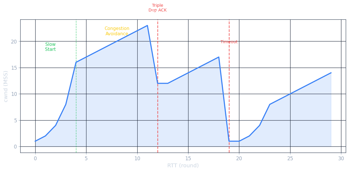
TCP uses an additive-increase, multiplicative-decrease (AIMD) algorithm together with slow start and congestion avoidance. The macroscopic view is a sawtooth: the congestion window grows linearly until a loss event, at which point it is cut in half and grows again. It has been proved mathematically that AIMD is the unique distributed algorithm that converges to efficient, fair bandwidth sharing at a bottleneck link — making AIMD not just an engineering heuristic but a principled design with theoretical foundations.
The sending rate is approximately \(\text{cwnd} / \text{RTT}\) bytes/second.
Slow start: cwnd begins at 1 MSS. For each ACK received, cwnd increases by 1 MSS. This doubles cwnd every RTT — exponential growth. The professor explains the name is a misnomer: the start is slow (1 MSS), but growth is fast. The idea is that we want to quickly find the available bandwidth without initially blasting the network. When cwnd reaches ssthresh (slow-start threshold), slow start ends.
Congestion avoidance: cwnd grows by 1 MSS per RTT (linear, additive increase). On a loss event detected by triple duplicate ACK, ssthresh = cwnd/2 and cwnd = ssthresh (TCP Reno enters fast recovery). On a timeout event, ssthresh = cwnd/2 and cwnd = 1 MSS, re-entering slow start.
TCP Tahoe vs. TCP Reno: Tahoe treats both timeout and triple-duplicate-ACK loss events identically — it always cuts cwnd to 1 MSS. Reno distinguishes them: triple-duplicate-ACK (a lighter congestion signal — subsequent packets got through, just one was lost) triggers halving and fast recovery rather than restarting slow start. Reno’s optimisation yields significantly higher average throughput.
where \(C = 0.4\) and \(\beta = 0.7\) (multiplicative decrease factor per RFC). TCP CUBIC has been the default in Linux since 2006 and is the most widely deployed congestion control algorithm on web servers.
Delay-based congestion control: instead of waiting for packet loss to signal congestion, it monitors RTT. The minimum observed RTT (\(RTT_{\min}\)) represents the uncongested RTT. The uncongested throughput is \(\text{cwnd} / RTT_{\min}\). If measured throughput approaches the uncongested estimate, the path is clear; if it falls well below, congestion is building. BBR (Bottleneck Bandwidth and RTT), developed by Google and deployed on its internal backbone, is the most prominent delay-based algorithm.
\[\text{average TCP throughput} = \frac{1.22 \cdot MSS}{RTT \cdot \sqrt{L}}\]where \(L\) is the packet loss probability.
TCP fairness: the professor provides an elegant geometric argument. Plot two TCP connections’ sending rates on a 2D graph. The equal-bandwidth line is at 45°; the full-utilisation line is where their sum equals \(R\). Starting from any point below the full-utilisation line, both connections increase linearly along a 45° line (additive increase). When the sum exceeds \(R\), both halve (multiplicative decrease). Successive iterations spiral toward the intersection of the two lines — equal sharing. This proves AIMD converges to fairness when connections share a bottleneck with equal RTTs.
ECN (Explicit Congestion Notification): two bits in the IP header’s Type of Service field are used. Congested routers set these bits to 11. The receiving TCP echoes this signal back to the sender via the ECE (ECN-Echo) bit in the TCP ACK. The sender halves cwnd and sets the CWR (Congestion Window Reduced) bit in its next segment to acknowledge the congestion signal. The result is the same congestion response but without packet drops — a gentler approach that avoids unnecessary retransmission overhead. ECN is particularly useful in data centre networks.
QUIC (Quick UDP Internet Connections): if the transport services needed by an application don’t fit either UDP or TCP, the application can implement its own protocol at the application layer on top of UDP. QUIC does exactly this. Originally designed by Google, QUIC is now widely deployed. It uses a single-RTT connection establishment combining security (TLS) and transport parameters. Each HTTP object is a separate stream within the QUIC connection; a lost UDP segment affects only the streams whose data was in that segment — no HOL blocking. QUIC also implements ACK-based reliable delivery and congestion control.
Chapter 4: The Network Layer — Data Plane
4.1 Overview of Network Layer
The primary role of the network layer is to move packets from a sending host to a receiving host. The professor distinguishes this from the transport layer: transport connects application processes end-to-end; network connects hosts hop-to-hop. The transport layer has protocol state only at the endpoints; the network layer has state (forwarding tables) at every router along the path.
Network-layer functions are present in every host and every router in the Internet — unlike transport and application protocols, which exist only at the endpoints. A router does not run a Web server or a TCP stack (in the data-plane sense); it does run IP, forwarding every packet that arrives regardless of application or protocol above.
Forwarding (data plane): moving a packet from a router’s input link to the appropriate output link — a per-router function implemented in hardware operating at nanosecond timescales. Analogy: driving through a single interchange.
Routing (control plane): determining the route or path taken by packets from sender to receiver — a network-wide function implemented in software operating at millisecond-to-second timescales. Analogy: planning the whole road trip.
The data plane determines how a datagram arriving at a router’s input link is forwarded to its output link. The control plane determines how a datagram is routed end-to-end. In the per-router control plane approach, routing algorithms run in each router and communicate with each other. In the Software-Defined Networking (SDN) control plane approach, a logically centralised controller computes and distributes forwarding tables to routers.
The Internet network layer provides a best-effort service: packets may be lost, reordered, or delayed with no guarantees on bandwidth, loss, or delay. The professor defends best-effort: a simple IP is easy to adopt; sufficient provisioning handles real-time applications; CDNs and data centres bring services close to users; TCP’s congestion control improves utilisation. It is hard to argue with the success of this model.
4.2 What’s Inside a Router
A router has four components: input ports, switching fabric, output ports, and a routing processor. The distinction between the routing processor (control plane, runs in software at millisecond timescales) and the switching fabric (data plane, runs in hardware at nanosecond timescales) mirrors the broader SDN distinction between control and data planes. Modern high-end routers (e.g., Cisco CRS series) have switching fabrics capable of 100 Tbps aggregate throughput; routing processors run sophisticated software implementing OSPF, BGP, and other protocols.
Input ports perform physical layer bit reception, link-layer frame extraction, and the lookup function: consult the forwarding table to determine the output port, then forward the packet into the switching fabric. To handle high line rates, the forwarding table is cached in the input port memory. Longest prefix matching determines the forwarding table entry — the entry with the longest matching prefix wins. This allows overlapping address ranges (more-specific routes override less-specific ones). TCAMs (Ternary Content-Addressable Memories) perform this match in a single clock cycle regardless of the table size — Cisco Catalyst routers have forwarding tables with up to a million entries.
Switching fabrics transfer packets from input ports to output ports. The switching fabric is the critical component that determines router throughput; its design is the subject of extensive research and engineering. Three types:
- Switching via memory: first-generation routers — CPU copies packets between I/O ports via shared memory bus; bandwidth limited to \(B/2\) (because every packet crosses the bus twice — once in, once out); cannot exploit multiprocessor parallelism easily.
- Switching via a bus: the input port sends the packet directly onto a shared bus, and the correct output port picks it up; bandwidth limited by bus speed; a contention mechanism selects which input port gets the bus at each cycle.
- Switching via an interconnection network: crossbar or multi-stage networks (e.g., Benes, Clos) allow multiple simultaneous non-conflicting transfers. Ideal rate: \(N \times R\) for \(N\) ports at rate \(R\). Modern high-speed routers use crossbar or multi-stage fabrics with fabric speedup (running the fabric faster than the line rate) to minimize head-of-line blocking.
Output port queuing occurs when packets arrive from the switching fabric faster than they can be transmitted on the outbound link. Head-of-line (HOL) blocking occurs at input queues: a queued packet must wait for transfer through the fabric even though its output port is free, because a packet at the head of the line goes to a congested port. HOL blocking limits the throughput of a crossbar switch to approximately 58% of the theoretical maximum.
Output buffer sizing: RFC 3439’s rule of thumb is \(\text{RTT} \times C\) where \(C\) is the link capacity. A more recent recommendation (2004) for \(N\) long-lived TCP flows: \(\text{RTT} \times C / \sqrt{N}\). The professor uses an analogy: buffering is like salt — too little and food is bland (link is underutilised), too much and it’s inedible (excessive delay, especially bad for real-time applications). The goal is to keep the bottleneck link busy without overflowing the buffer.
Packet scheduling determines transmission order:
- FIFO: first-in, first-out.
- Priority queuing: packets classified into priority classes; higher-priority classes served first. Low-priority packets may starve.
- Round robin: classes served cyclically, one packet at a time — fair but no priority.
- Weighted fair queuing (WFQ): generalised round robin with weights \(w_i\), giving class \(i\) a share of bandwidth proportional to \(w_i / \sum w_j\). Implements per-class minimum bandwidth guarantees.
4.3 The Internet Protocol (IP): IPv4, Addressing, IPv6
IP is the “narrow waist” of the Internet protocol stack. Above IP lie many transport and application protocols (TCP, UDP, HTTP, SMTP, DNS). Below IP lie many link-layer technologies (Ethernet, WiFi, fiber, DSL, 5G). IP itself is a single protocol — every packet, regardless of application or link technology, must be an IP datagram. This unifying property is what makes the Internet work: any application can use any link technology, as long as both can speak IP. The professor notes that IP is intentionally simple and minimal — its “best-effort” service model offloads complexity to the endpoints.
IPv4 datagram format — minimum 20-byte header:
| Field | Size | Description |
|---|---|---|
| Version | 4 bits | IP version (4) |
| Header length | 4 bits | Header length in 32-bit words |
| Type of service | 8 bits | Differentiated services / ECN |
| Datagram length | 16 bits | Total length (header + data) in bytes |
| Identifier | 16 bits | Used for fragmentation |
| Flags | 3 bits | Fragmentation control |
| Fragmentation offset | 13 bits | Position of fragment |
| TTL | 8 bits | Decremented by each router; datagram dropped at 0 |
| Protocol | 8 bits | Transport protocol (6=TCP, 17=UDP) |
| Header checksum | 16 bits | Error detection (recomputed at every router) |
| Source IP address | 32 bits | |
| Destination IP address | 32 bits |
IP fragmentation and reassembly: links have a maximum transmission unit (MTU) limiting the largest IP datagram. Large datagrams are fragmented at intermediate routers into multiple smaller datagrams with the same identification number, appropriate fragment offsets, and flags. Reassembly is performed only at the destination host. IPv6 eliminates fragmentation to speed up router processing.
IPv4 addressing: each interface has a 32-bit IP address. A subnet is a set of interfaces that can physically reach each other without passing through an intervening router. The subnet mask (e.g., /24 in CIDR notation) indicates how many bits define the subnet.
CIDR (Classless Inter-Domain Routing): the Internet address assignment strategy. An IP address has the form a.b.c.d/x, where x is the number of bits in the network prefix. This replaced classful addressing (class A /8, class B /16, class C /24). CIDR enables route aggregation: an ISP that has been allocated 200.23.16.0/20 can advertise a single prefix to the Internet even if it has assigned 8 different /23 blocks to different organisations.
DHCP (Dynamic Host Configuration Protocol) allows a host to obtain an IP address automatically. It uses UDP. The four-step interaction:
- DHCP discover: newly arriving host broadcasts to
255.255.255.255on UDP port 67. - DHCP offer: server responds with an offered IP address and configuration.
- DHCP request: client sends a request for the offered address.
- DHCP ACK: server confirms; provides IP address, subnet mask, default gateway, and DNS server address.
DHCP is used not just by end hosts but also by routers: when a router’s WAN interface connects to the ISP, it receives its public IP address via DHCP from the ISP’s DHCP server.
Network Address Translation (NAT) allows a home/enterprise network to use private IP addresses internally, appearing to the outside world as having a single IP address. The NAT translation table maps (WAN-side IP, WAN-side port) to (LAN-side IP, LAN-side port). When a packet leaves the home network, NAT replaces the source IP/port; when a packet arrives from the Internet, NAT restores the original destination IP/port.
IPv6 was developed to address IPv4 address exhaustion. Key features: 128-bit addresses (\(2^{128}\) addresses — enough to assign an IP address to every grain of sand on Earth many times over), fixed 40-byte header (no fragmentation fields in the base header — moved to extension headers; no checksum — speeds up router processing), anycast address (deliver to nearest of a group), flow label field (for QoS). No header checksum field means routers no longer need to recompute the checksum after decrementing the hop limit — a significant speedup at line rate.
IPv6 addresses are written in colon-separated hexadecimal groups: e.g., 2001:0db8:0000:0000:0000:0000:0000:0001, often compressed to 2001:db8::1. The loopback address is ::1 (equivalent to IPv4’s 127.0.0.1). The link-local prefix fe80::/10 is used for addresses that are automatically configured on every interface and are used for neighbour discovery (the IPv6 replacement for ARP).
The professor explains why IPv6 adoption has been so slow: unlike ARPANET’s 1983 “flag day” (where all nodes were simultaneously switched from NCP to TCP/IP), the Internet is too large to turn off and restart. Instead, IPv6 has been deployed gradually through tunneling: IPv6 datagrams are encapsulated as the payload of IPv4 datagrams, allowing them to pass through IPv4-only routers. Both the entry and exit routers of the tunnel have dual IPv4/IPv6 stacks. According to Google, around 30% of users access Google services via IPv6, and about one-third of US government domains are IPv6-capable — but this adoption rate is far lower than the IETF envisioned 25 years ago.
4.4 Generalized Forwarding and SDN
In generalized forwarding, each router/switch has a flow table computed and distributed by a logically centralised routing controller. This represents a fundamental shift in the network architecture: instead of each device independently running routing algorithms and making forwarding decisions, a single controller has a network-wide view and programs every device’s forwarding behaviour. The analogy is moving from a distributed group of taxi drivers each planning their own route, to a centralised traffic management system that plans routes for all taxis simultaneously with full knowledge of road conditions. Each entry has: match fields (header values to match against any combination of link, network, or transport layer headers), counters (updated for each matching packet), and actions (forward, drop, modify header, send to controller).
OpenFlow (version 1.0) is the pioneering generalized forwarding protocol. Match fields include: ingress port, Ethernet source/destination/type, IP source/destination/protocol, TCP/UDP source/destination port. Actions include: forward to port(s), drop, modify header fields (VLAN tag, TCP source port, IP destination for NAT), send-to-controller for further processing.
The match-plus-action abstraction is powerful:
- Router: match on longest IP destination prefix → forward to output link
- Switch: match on destination MAC → forward to output link or flood
- Firewall: match on IP addresses and TCP/UDP ports → permit or deny
- NAT: match on IP/port → rewrite IP/port
The power of SDN: separation of data plane (packet forwarding) and control plane (routing decisions), flow-based forwarding (based on any combination of header fields), and logically centralised control with a programmable controller enabling rapid software innovation without touching hardware.
Chapter 5: The Network Layer — Control Plane
5.1 Introduction
The network-layer control plane provides the per-router mechanism for determining how datagrams are routed among the routers along an end-to-end path. The control plane is what populates the forwarding tables that the data plane uses to forward packets. Two approaches: per-router control (traditional; routing algorithms run in each router, communicating with neighbour routers) and logically centralised control (SDN; a centralised controller computes and distributes forwarding tables).
The fundamental challenge of routing is scale. The Internet has hundreds of thousands of routers. For every router to know a route to every other router using a flat routing architecture would require storing and updating millions of routes, and flooding routing update messages would consume all available bandwidth. The solution is hierarchical routing — organising routers into Autonomous Systems and using different routing protocols (OSPF for intra-AS, BGP for inter-AS) at each level of the hierarchy.
5.2 Routing Algorithms
A routing algorithm determines the best path from senders to receivers through the network of routers. The professor frames the goal: given a network modelled as a graph where nodes are routers and edges are links, find the minimum-cost path from a source to all destinations. “Cost” can represent anything — monetary cost, propagation delay, congestion, or simply hop count. In practice, OSPF uses a configurable metric (often inversely proportional to bandwidth) while BGP uses policy attributes.
Routing algorithms can be classified along two dimensions. Centralised vs. decentralised: a centralised algorithm (like link-state) computes the shortest path with complete, global knowledge of the graph. A decentralised algorithm (like distance-vector) computes routes iteratively, with each node knowing only the costs to its directly attached neighbours. Static vs. dynamic: static routing changes rarely (routes are manually configured); dynamic routing adjusts as network conditions change. The network is modelled as a graph \(G = (N, E)\) where \(N\) is the set of nodes (routers) and \(E\) is the set of edges (links), each with a cost. The least-cost path between two nodes is the path whose sum of link costs is minimum.
Link-state (LS) routing: each node broadcasts link-state packets containing link identities and costs to all nodes, so every node has an identical, complete view of the network graph. Dijkstra’s shortest-path algorithm is then run locally:
Initialize: D(v) = ∞ for all v ≠ u
            D(u) = 0
            S = {}
Loop:
    Find w not in S with minimum D(w)
    Add w to S
    For each neighbor v of w not in S:
        D(v) = min(D(v), D(w) + c(w,v))
Until all nodes in S
Complexity: \(O(N^2)\) naively, \(O(N \log N)\) with a heap. A problem with LS routing is oscillations: if link costs depend on traffic volume, all routers simultaneously compute new routes after a traffic change, potentially causing routes to oscillate. The professor walks through a concrete example: four routers A, B, C, D. Initial routes all route traffic one way; after recomputation everyone shifts to the other side; the oscillation can repeat indefinitely.
\[d_x(y) = \min_v \{ c(x,v) + d_v(y) \}\]DV routing is distributed: each node only communicates with directly attached neighbours. It is iterative: the process continues until no more distance vector changes occur.
A key problem with DV routing is the count-to-infinity problem: when a link cost increases dramatically or a link fails, it can take many iterations for the bad news to propagate, during which time routing loops can form. The professor calls this the “good news travels fast, bad news travels slow” asymmetry. Poisoned reverse is a partial fix: if node \(z\) routes through \(y\) to reach \(x\), then \(z\) advertises to \(y\) that its distance to \(x\) is infinity. This prevents the two-node loop, but cannot fix loops involving three or more nodes.
Comparison of LS and DV:
| Property | Link State | Distance Vector |
|---|---|---|
| Message complexity | \(O(NE)\) messages | Exchange only with neighbours |
| Speed of convergence | \(O(N^2)\) steps | Slower; count-to-infinity possible |
| Robustness | A misconfigured node corrupts its own routing only | Errors propagate to all nodes |
5.3 Intra-AS Routing in the Internet: OSPF
The Internet organises routers into Autonomous Systems (ASes) — each AS consists of a group of routers under the same administrative control. An AS is identified by a unique 16-bit (or 32-bit in the extended format) AS number (ASN); for example, the University of Waterloo has its own ASN, as does every major ISP and content provider. Routers within the same AS run the same intra-AS routing protocol. Two most prevalent intra-AS routing protocols: RIP (distance-vector, DVs exchanged every 30 seconds, legacy) and OSPF (link-state, the dominant choice).
The professor explains the motivation for ASes: it is not feasible for every Internet router to know a route to every other router — the forwarding tables would be enormous and the routing update traffic would saturate links. Scaling requires hierarchical routing. Additionally, each autonomous system wants to control its own routing policies. An ISP does not want its competitor’s traffic routing through its backbone; a university wants to control which paths packets traverse through its campus.
OSPF: a link-state protocol where each router constructs a complete topological map of the entire AS and then runs Dijkstra’s to determine the shortest path tree. Topological information is flooded by sending OSPF link-state advertisements (LSAs) to all routers in the AS. OSPF messages are encapsulated directly in IP datagrams (protocol number 89) — it bypasses UDP and TCP and uses its own reliable flooding mechanism. OSPF maintains neighbour relationships through periodic hello messages; if hello messages stop arriving, the link is declared down and LSAs are flooded to notify all other routers of the change. OSPF converges quickly — typically within a few seconds of a topology change — making it suitable for enterprise and ISP networks where rapid failover is important.
OSPF advantages over simpler protocols: authentication (all OSPF messages can be authenticated against malicious or misconfigured routers), multiple same-cost paths (OSPF can load-balance across them), support for unicast and multicast routing, and hierarchical OSPF with a two-level hierarchy (local areas and a backbone area 0). Area border routers (ABRs) connect local areas to the backbone; they summarise prefixes from their area to reduce the size of routing tables in other areas. Autonomous system boundary routers (ASBRs) connect the OSPF domain to other routing systems (e.g., BGP). Within a broadcast network (like Ethernet), OSPF elects a designated router (DR) and a backup DR to reduce the number of LSA flooding messages — without a DR, every router would exchange LSAs with every other, causing \(O(N^2)\) flooding.
5.4 Routing Among the ISPs: BGP
While intra-AS routing optimises cost, inter-AS routing is dominated by policy concerns. BGP (Border Gateway Protocol) is the de facto standard inter-AS routing protocol — the professor calls it “the glue that holds the Internet together.” BGP was first standardised in 1989 and is currently at version 4 (RFC 4271). Despite its age, BGP’s fundamental design has proven remarkably durable. The Internet’s entire inter-domain routing infrastructure runs on a protocol that fits in a single RFC. This resilience is both BGP’s greatest strength and its greatest weakness: the simplicity that makes it deployable also limits its expressiveness and makes some security improvements difficult to retrofit.
BGP provides each AS the means to: (1) obtain subnet reachability information from neighbouring ASes via eBGP sessions, (2) propagate reachability information to all internal routers via iBGP sessions, (3) determine good routes based on reachability and policy.
BGP pairs exchange routing information over semi-permanent BGP sessions on TCP port 179. BGP is a path-vector protocol: advertisements include the full path of ASes, allowing loop detection. Using the full AS path (not just the next hop as in distance-vector) is crucial — if an AS appears in the path of a received advertisement, the receiving AS knows that accepting this route would create a routing loop and rejects it. This is how BGP achieves loop-free routing at global scale.
BGP route attributes: AS-PATH (the list of ASes through which the advertisement has passed — used for loop detection), NEXT-HOP (the IP address of the router interface that begins the AS-PATH). A route in BGP is a prefix plus attributes.
Hot potato routing: among multiple BGP-advertised paths to the same destination, a router selects the path whose NEXT-HOP router has the lowest cost within the AS (closest NEXT-HOP) — minimising intra-AS cost and “getting rid of” the packet as quickly as possible, regardless of inter-AS costs beyond the boundary. The analogy: a hot potato is unpleasant to hold, so you toss it to the nearest exit as fast as possible.
Route selection order: (1) highest local preference value (locally configured policy), (2) shortest AS-PATH, (3) closest NEXT-HOP router (hot potato), (4) BGP identifier as tiebreaker.
The professor walks through the policy motivation with a three-ISP example. ISP B has customers W and is connected to ISPs A and C. B advertises the route B-A-W to C, meaning “you can reach W via me through A.” But B chooses not to forward the route from C to A — because B gets no revenue from routing C’s traffic to A to reach W. B is not willing to be a free transit backbone for C. Similarly, a multi-homed customer X connected to both B and C will not forward B’s traffic to C because X would be acting as a free transit ISP. This policy enforcement — carrier-grade economic logic baked into BGP local-preference settings — is why BGP is sometimes called a “policy-based” routing protocol rather than a “shortest-path” routing protocol.
IP-anycast uses BGP to advertise the same IP address from multiple locations; BGP’s shortest-path selection automatically routes a client to the nearest server. Used by DNS root servers and CDNs.
5.5 The SDN Control Plane
In an SDN architecture, the control-plane functions are moved to an external logically centralised controller. The professor frames the motivation historically: before SDN (circa 2005), networking was dominated by closed, proprietary, monolithic routers from companies like Cisco running proprietary OS implementations. Standalone proprietary hardware middle-boxes performed firewalling, load balancing, and NAT. This ossification made innovation slow and expensive. A network operator who wanted to implement a new routing policy had to convince vendors to add a feature in the next hardware generation — a process that could take years and cost millions. With SDN, the same operator writes a short Python program to the controller API and deploys it in minutes.
SDN was pioneered by researchers at Stanford and UC Berkeley around 2005–2008, with the OpenFlow protocol introduced in 2008. Today, major cloud providers (Google, Amazon, Microsoft) and carriers use SDN internally to manage their data centre networks and wide-area backbones. Google’s B4 WAN, announced in 2013, was one of the first large-scale SDN deployments, achieving near-100% WAN link utilisation (vs. the industry average of ~30–40%) by centrally managing traffic engineering across all backbone links.
SDN’s four key features: (1) generalised flow-based forwarding (via OpenFlow), (2) separation of the control and data planes, (3) network programmability through control applications, (4) open interfaces and commodity switching hardware.
The SDN controller architecture has three layers: (1) a communication layer implementing the southbound API (e.g., OpenFlow) to communicate with data-plane switches, (2) a network-wide state-management layer maintaining the network graph, flow tables, and statistics, (3) the northbound interface toward network-control applications (route computation, access control, load balancing). Controllers such as OpenDaylight and ONOS implement these layers.
OpenFlow protocol operates between the controller and a switch, using TCP (optionally TLS). Controllers listen on port 6653. Messages: controller-to-switch (feature request, configure, modify-state, packet-out), switch-to-controller (packet-in when no match, flow-removed, port-status), and symmetric (hello, echo request/reply).
5.6 ICMP: The Internet Control Message Protocol
ICMP is used by hosts and routers to communicate network-level information, primarily error reporting. ICMP is often called the “error protocol” of the Internet. When something goes wrong in the network — a TTL expires, a destination is unreachable, a fragmentation is required — ICMP is the mechanism by which the network notifies the sender. Without ICMP, the sender would simply observe that packets stop arriving, with no indication of why. ICMP messages are carried in IP datagrams (protocol number 1). An ICMP message has a type, code, and the first 8 bytes of the triggering IP datagram.
Common ICMP message types:
| Type | Code | Description |
|---|---|---|
| 0 | 0 | Echo reply (ping response) |
| 3 | 0 | Destination network unreachable |
| 3 | 1 | Destination host unreachable |
| 3 | 3 | Destination port unreachable |
| 4 | 0 | Source quench (deprecated) |
| 8 | 0 | Echo request (ping) |
| 11 | 0 | TTL expired (used by traceroute) |
Traceroute works by sending probes with incrementally increasing TTL values (starting at 1). Each router that decrements TTL to 0 discards the datagram and returns an ICMP “time exceeded” message (type 11, code 0) including its IP address. The source records the RTT and the router’s address. By sending a final datagram to an unlikely high-numbered port, the destination host returns an ICMP “port unreachable” message (type 3, code 3), signalling that the destination has been reached and the traceroute should stop. Three probes are sent at each TTL value, so three RTT measurements appear per hop.
ICMP is also used by routers to implement source quench (now deprecated) and by hosts to perform path MTU discovery: send large datagrams with the “Don’t Fragment” (DF) bit set; any router that would need to fragment returns an ICMP “fragmentation needed” (type 3, code 4) message with the MTU of the link that cannot carry the datagram. The source can then adjust its datagram size to avoid fragmentation along the path.
Chapter 6: The Link Layer and LANs
6.1 Introduction to the Link Layer
The link layer is responsible for transferring a datagram from one node to an adjacent node over a single communication link. It is the last protocol layer before data hits the physical wire, optical fiber, or radio channel. The professor observes that the link layer has the most diversity of any layer in the protocol stack: the physical and link-layer technologies in use today span coaxial cable from the 1970s to 5G millimetre-wave radio, yet the Internet treats them all as interchangeable “wires” thanks to the IP abstraction. A network engineer must understand link-layer technologies because performance and reliability often live here — most end-to-end packet loss happens on wireless links, not in the core, and most access-link bottlenecks are link-layer constraints. The professor uses a transportation analogy: consider travelling from Waterloo to Lausanne, Switzerland. A limousine takes you from Waterloo to Pearson Airport; a plane from Pearson to Geneva; a train from Geneva to Lausanne. Each segment is managed by a different company using a different mode of transport. You are the datagram; each transportation segment is a link; the transportation mode is the link-layer protocol; the travel agent is the routing protocol. Each segment provides the basic service of moving you from one location to an adjacent one.
Link-layer services include: framing (encapsulating a network-layer datagram in a link-layer frame), link access (a MAC protocol coordinates frame transmissions on shared medium), reliable delivery (guaranteed delivery over the link, often used for high bit-error-rate wireless links; many wired link protocols do not provide this — it would be unnecessary overhead for low-BER links), error detection and correction (hardware-implemented, more powerful than IP/UDP/TCP checksums).
The link layer is implemented in a network adapter (NIC — network interface card), which is a combination of hardware, software, and firmware. Most link-layer functionality is in hardware on a special-purpose chip. Software components handle higher-level functions like assembling addressing information, responding to controller interrupts, and passing datagrams to the network layer. The link layer is thus a partnership of hardware and software.
6.2 Error-Detection and Correction Techniques
Bit errors in a transmitted frame occur when a 1 is misinterpreted as 0 (or vice versa) due to signal attenuation, electromagnetic noise, or other interference. The link layer provides mechanisms to detect, and sometimes correct, these errors. Error detection is implemented in hardware — at link rates of Gbps, there is no time for software-based error checking on every frame. The three main techniques used in practice are parity checks, checksums, and cyclic redundancy checks.
Parity bits: a single parity bit allows detection of any odd number of bit errors. A two-dimensional parity scheme can both detect and correct single-bit errors.
Checksum: bytes of the data are treated as 16-bit integers and summed; the 1s-complement of the sum forms the checksum. Used in IP, UDP, TCP.
Cyclic Redundancy Check (CRC): a more powerful error-detection technique. The sender and receiver agree on a \((r+1)\)-bit generator polynomial \(G\). The sender appends \(r\) CRC bits to the \(d\)-bit message such that the resulting \((d+r)\)-bit pattern is exactly divisible by \(G\) using modulo-2 arithmetic. The receiver divides the received \(d+r\) bits by \(G\); if the remainder is non-zero, an error is detected. CRC can detect all burst errors of fewer than \(r+1\) bits. Used in Ethernet, WiFi, ATM.
6.3 Multiple Access Links and Protocols
Communication links are either point-to-point (a single sender and receiver at each end) or broadcast links (multiple sending and receiving nodes connected to the same shared broadcast channel). When multiple nodes transmit simultaneously on a broadcast channel, a collision occurs and all frames involved are garbled. The multiple access problem is central to the design of shared-medium networks like WiFi and classic Ethernet.
The professor uses a cocktail-party analogy: everyone shares the same “broadcast medium” (the air). We have evolved protocols — don’t interrupt, raise your hand in class, wait until spoken to. Computer networks similarly need multiple access protocols. A key observation is that these protocols must be implemented in a completely distributed fashion: there is no central coordinator telling nodes when to transmit. Each node must locally decide, based only on what it observes about the channel, when it is allowed to transmit.
A desirable multiple access protocol for a channel of rate \(R\) bps should: (1) give a single active node throughput \(R\); (2) give \(M\) active nodes throughput \(R/M\) each on average; (3) be decentralised (no single point of failure); (4) be simple and inexpensive to implement.
Channel partitioning protocols: divide the channel into pieces.
- TDMA (Time-Division Multiple Access): allocates time slots cyclically. Fair, collision-free, but wastes capacity when fewer than \(N\) nodes are active — a node is limited to \(R/N\) even if it is the only active node. In the picture, three out of six slots are wasted because stations 2, 5, and 6 are idle; station 3 must wait for station 2’s time slot even though station 2 is idle.
- FDMA (Frequency-Division Multiple Access): allocates frequency bands. Same advantages and disadvantages as TDMA.
Random access protocols: always transmit at full rate \(R\); on collision, nodes retransmit after a random delay.
- Slotted ALOHA: time is divided into slots of \(L/R\) seconds. A node transmits at the start of a slot; if collision, retransmit in a subsequent slot with probability \(p\). Maximum efficiency: \(1/e \approx 0.37\). This means that in the best case, only 37% of slots actually carry successful transmissions.
- Pure ALOHA: no synchronisation required. Maximum efficiency: \(1/(2e) \approx 0.18\). The halving compared to slotted ALOHA is because a transmission at time \(t\) can collide with a transmission that started in the interval \([t-1, t]\).
- CSMA (Carrier Sense Multiple Access): “listen before talking.” If the channel is idle, transmit; if busy, defer. Collisions still occur due to propagation delay: node D may sense the channel idle even though B has already started transmitting — B’s bits have not yet reached D. The longer the physical channel, the greater the propagation delay and the higher the collision rate.
- CSMA/CD (CSMA with Collision Detection): transmitting nodes also listen while transmitting; on detecting a collision, abort the transmission immediately. Used in Ethernet. After aborting, use binary exponential backoff: after the \(n\)th collision, wait a random number of time slots from \(\{0, 1, \ldots, 2^n - 1\}\). After 10 collisions the range freezes at 1023 slots; after 16 consecutive collisions the adapter gives up and reports an error. If node A and node D transmit simultaneously and detect the collision, both stop and wait a random time: A might wait 0 slots, D might wait 1 slot. A retransmits first; if D’s timer hasn’t expired yet, D senses the channel busy and defers.
- CSMA/CA (CSMA with Collision Avoidance): used in wireless LANs (IEEE 802.11) instead of CSMA/CD because wireless adapters cannot detect a collision while transmitting — the transmitted signal overwhelms the weak received signal. CSMA/CA uses a different strategy to avoid collisions proactively.
Taking-turns protocols: eliminate collisions and empty slots.
- Polling: a master node polls each node in round-robin fashion. Eliminates collisions; reduces throughput due to polling delay and is vulnerable to master node failure.
- Token passing: a token frame circulates; a node can transmit only when holding the token. Decentralised; vulnerable to token loss (if a node crashes while holding the token, a recovery procedure is needed). Used in FDDI and 802.5 Token Ring.
6.4 Switched Local Area Networks
In a switched LAN, a link-layer switch connects end systems and provides collision-free, dedicated bandwidth to each device. Unlike the old hub-based Ethernet where all devices shared a single collision domain, each switch port gets a dedicated full-duplex channel to its connected device. This means that two computers connected to different ports of a switch can simultaneously transmit at full link rate without collision.
MAC addresses (also called LAN addresses or physical addresses) are 48-bit identifiers (6 bytes), typically written in hexadecimal (e.g., 1A-23-F9-CD-06-9B). MAC addresses are flat — they do not change based on location, analogous to a social security number that follows a person regardless of address. The broadcast MAC address FF-FF-FF-FF-FF-FF reaches all adapters on the LAN. IEEE manages the MAC address space; organisations purchase blocks of \(2^{24}\) addresses (first 24 bits fixed, last 24 bits assigned by the manufacturer). Unlike IP addresses (which change subnet-to-subnet), a MAC address stays the same whether a laptop is in the classroom or at Starbucks.
ARP (Address Resolution Protocol) translates IP addresses to MAC addresses within a subnet. Each host and router has an ARP table mapping IP addresses to MAC addresses (with TTLs — typically 20 minutes). ARP is plug-and-play: the table is built automatically.
When host A wants to send a datagram to host B on the same subnet but doesn’t know B’s MAC address, A broadcasts an ARP query (to FF-FF-FF-FF-FF-FF) containing B’s IP address. B recognises its own IP and responds with a ARP reply (unicast) containing its MAC address. A caches this mapping.
When A wants to send a datagram to host B on a different subnet, A sends the datagram in a frame addressed to the first-hop router’s MAC address (obtained via ARP on the router’s IP address, which A learned from DHCP). The router receives the frame, strips the frame header, reads the IP datagram’s destination, consults its forwarding table, and re-encapsulates the datagram in a new frame with the next-hop’s MAC address. This process repeats hop by hop.
6.5 Ethernet
Ethernet is by far the most widely used wired LAN technology. The professor calls it “for local area networking what IP is for global networking.” It was invented at Xerox PARC in the 1970s by Bob Metcalfe and David Boggs, and has survived and thrived through multiple technological generations by maintaining backward-compatible frame formats while dramatically increasing speeds. The original 10 Mbps shared coaxial cable Ethernet has been succeeded by 100 Mbps, 1 Gbps, 10 Gbps, and 100 Gbps variants, all sharing the same fundamental frame format. This backward compatibility is a key reason for Ethernet’s dominance — infrastructure upgrades can be done incrementally without replacing everything at once. It was invented in the mid-1970s using a coaxial bus (CSMA/CD); by the late 1990s, hubs replaced the bus (still a broadcast domain, collision detection still needed); by the early 2000s, layer-2 switches replaced hubs (store-and-forward, collision-free, full-duplex). Modern switched Ethernet essentially never needs CSMA/CD.
Ethernet comes in many flavours standardised by IEEE 802.3: 10 Mbps (10BASE-T), 100 Mbps (Fast Ethernet, 100BASE-TX over copper, 100BASE-FX over fiber), 1 Gbps (Gigabit Ethernet), 10 Gbps (10GBASE). The format of the Ethernet frame has remained constant across all variants — the “timeless centrepiece” of the standard.
Ethernet frame structure (minimum 64 bytes, maximum 1518 bytes):
| Field | Size | Description |
|---|---|---|
| Preamble | 7 bytes | 10101010... for clock synchronisation |
| SFD | 1 byte | 10101011 — start frame delimiter |
| Destination MAC | 6 bytes | |
| Source MAC | 6 bytes | |
| Type/Length | 2 bytes | Network-layer protocol (e.g., 0x0800 for IP, 0x0806 for ARP) |
| Data (payload) | 46–1500 bytes | Network-layer datagram; padded to 46 bytes if shorter |
| CRC | 4 bytes | Error detection |
Ethernet is connectionless (no handshaking before sending a frame) and unreliable (dropped frames are not retransmitted by Ethernet itself; higher-layer protocols handle this). If a frame fails the CRC check, the adapter simply discards it — no NAK is sent, no notification given. The stream of datagrams passed to the network layer may therefore have gaps, handled by TCP if the application uses it.
The minimum frame size of 64 bytes is not arbitrary — it is set so that the frame transmission time is at least twice the propagation delay across the maximum Ethernet segment. This ensures that the transmitter is still sending when a collision signal from the far end of the cable arrives, guaranteeing that CSMA/CD can detect collisions correctly. This constraint limits the maximum cable length for classic Ethernet: 500 metres for 10 Mbps (because at that speed 64 bytes takes 51.2 μs to transmit, and round-trip propagation at 2×10⁸ m/s over 500 m is 5 μs — well within the frame time).
6.6 Link-Layer Switches
A link-layer switch receives incoming frames and forwards them to outgoing links. Switches are transparent to hosts and routers — no special configuration is needed. They are plug-and-play: no intervention from a network administrator. This plug-and-play property, combined with the self-learning algorithm, means that a network administrator can install a new switch simply by connecting cables — the switch will automatically learn the topology without any configuration. This is a significant operational advantage over routers, which require manual IP address configuration and routing protocol setup.
Self-learning: the switch table is built automatically. For each incoming frame, the switch records: (1) the MAC address in the frame’s source address field, (2) the interface from which the frame arrived, (3) the current time. Entries are deleted after an aging time (e.g., 60 minutes).
Forwarding logic:
- If the destination MAC has no entry in the table → flood (forward on all interfaces except the incoming one).
- If the destination MAC maps to the same interface the frame arrived on → filter (discard the frame — the destination is on the same segment).
- If the destination MAC maps to a different interface → forward to that interface.
Switches vs. routers: both are store-and-forward devices. Switches are layer-2 (MAC addresses), plug-and-play, no routing algorithm needed. Routers are layer-3 (IP addresses), require configuration, run routing algorithms. For small networks (tens to hundreds of hosts), switches suffice and are simpler. For large networks, routers provide better isolation (broadcast storms can paralyse a large switched network) and can find optimal paths.
VLANs (Virtual Local Area Networks) allow a single physical switch to act as multiple disjoint virtual switches. Ports are grouped into VLANs; frames from one VLAN cannot reach another VLAN without going through a router. Motivations: (1) efficiency — broadcast traffic (ARP, DHCP, switch flooding) is confined to the VLAN, not sent to all hosts; (2) security — traffic is isolated between groups; (3) flexibility — a user can be logically associated with a VLAN even if physically relocated (e.g., a CS user whose office moves to the EE building but who still needs to appear on the CS VLAN and not the EE VLAN).
Port-based VLANs assign physical switch ports to VLANs in management software. To span VLANs across multiple physical switches, a trunk port links the switches and carries frames tagged with the 802.1Q VLAN ID — a 2-byte tag inserted between the source MAC and type fields of the Ethernet frame.
6.7 Retrospective: A Day in the Life of a Web Page Request
Consider what happens when a student opens a laptop in a university network and browses to www.google.com. This scenario ties together all layers of the protocol stack. The professor uses this “day in the life” walkthrough to demonstrate that every concept in the course — DHCP, ARP, DNS, TCP, HTTP, Ethernet, IP routing — is a necessary part of the system. Remove any one of them and the page does not load.
Step 1 — DHCP: the laptop broadcasts a DHCP discover message within a UDP datagram → IP datagram → Ethernet frame (destination: broadcast FF-FF-FF-FF-FF-FF). The frame is flooded by the switch. The DHCP server (running on the first-hop router) sees the broadcast and responds with a DHCP ACK containing: the laptop’s IP address, the subnet mask, the IP address of the first-hop router, and the name and IP of the local DNS server. The laptop decapsulates all layers and records this information.
Step 2 — ARP: to send the DNS query, the laptop needs the MAC address of the first-hop router. It sends an ARP query (broadcast). The router replies with its MAC address. The laptop caches this mapping.
Step 3 — DNS: the laptop creates a DNS query for www.google.com and sends it via UDP to the local DNS server. The query is encapsulated in a UDP datagram → IP datagram → Ethernet frame destined to the first-hop router’s MAC. The frame crosses the campus LAN to the router, which routes the IP datagram to the DNS server (potentially via BGP and OSPF). The DNS server returns the IP address of www.google.com.
Step 4 — TCP and HTTP: with the IP address, the laptop initiates a TCP connection (SYN → SYNACK → ACK, three-way handshake) to Google’s server at port 80. In practice, modern browsers use HTTPS (port 443) and perform a TLS handshake as well, adding 1–2 more round trips before data flows. An HTTP GET request is sent over the connection. The HTTP response returns the web page content. The browser renders the page, making additional HTTP requests for embedded objects (CSS, images, JavaScript).
The entire sequence from connecting to the WiFi to receiving the first byte of the web page involves: DHCP (1 RTT), ARP (1 RTT), DNS (1–3 RTTs), TCP handshake (1 RTT), TLS handshake (1–2 RTTs), HTTP GET (1 RTT). That is 6–9 round trips of latency before any visible content arrives. On a campus WiFi with 5 ms RTT to the gateway, this is 30–45 ms — imperceptibly fast. On a satellite link with 600 ms RTT, this would take 3.6–5.4 seconds just to load the first byte of the page. This is why minimising round trips is the central goal of web performance engineering.
Throughout this journey, every packet carries multiple header layers: Ethernet frame at the link layer, IP datagram at the network layer, TCP segment at the transport layer, HTTP message at the application layer — all wrapped in each other by encapsulation. Each header is read and processed by the appropriate layer at each node; routers process only IP headers; switches process only Ethernet headers; end hosts process all layers.
The professor closes the course by noting that this journey through all five layers of the Internet protocol stack is now complete, and what was once invisible — the DHCP discovery, the ARP queries, the DNS resolution, the TCP handshake, the BGP route selection — is now a fully understood chain of protocols. The Internet’s apparent magic dissolves into a disciplined hierarchy of simple protocols, each doing one job well, stacked to deliver extraordinary complexity.
TCP State Machine Summary
TCP connections pass through a well-defined sequence of states. Understanding the state machine helps debug connection issues and understand protocol behaviour.
Client-side TCP state transitions (initiating connection):
CLOSED
  │  [app: connect()]
  ▼  sends SYN
SYN_SENT
  │  receives SYNACK, sends ACK
  ▼
ESTABLISHED   ← data transfer occurs here
  │  [app: close()]
  ▼  sends FIN
FIN_WAIT_1
  │  receives ACK
  ▼
FIN_WAIT_2
  │  receives FIN, sends ACK
  ▼
TIME_WAIT  (waits 2*MSL)
  │
  ▼
CLOSED
Server-side TCP state transitions (accepting connection):
CLOSED
  │  [app: bind(), listen()]
  ▼
LISTEN
  │  receives SYN, sends SYNACK
  ▼
SYN_RCVD
  │  receives ACK
  ▼
ESTABLISHED   ← data transfer occurs here
  │  receives FIN, sends ACK
  ▼
CLOSE_WAIT
  │  [app: close()]
  ▼  sends FIN
LAST_ACK
  │  receives ACK
  ▼
CLOSED
The TIME_WAIT state (client side after active close) lasts 2 × MSL (Maximum Segment Lifetime, typically 60 seconds). Its purpose is to ensure the final ACK reaches the server even if it is lost (triggering server retransmission of FIN), and to allow old duplicate segments from this connection to expire before a new connection on the same four-tuple is established.
Protocol Summary Tables
The following tables summarise the key protocols covered in this course, organised by layer and function.
Application Layer Protocols
| Protocol | Port | Transport | Purpose |
|---|---|---|---|
| HTTP/1.1 | 80 | TCP | Web page transfer |
| HTTPS | 443 | TCP | Secure web (HTTP + TLS) |
| HTTP/3 | 443 | UDP (QUIC) | Modern web, no HOL blocking |
| SMTP | 25 | TCP | Email sending (push) |
| IMAP | 143 | TCP | Email retrieval (keep on server) |
| POP3 | 110 | TCP | Email retrieval (download) |
| DNS | 53 | UDP (TCP for large) | Name → IP resolution |
| FTP | 21/20 | TCP | File transfer |
| SSH | 22 | TCP | Secure remote shell |
Transport Layer Comparison
| Feature | TCP | UDP |
|---|---|---|
| Connection setup | 3-way handshake | None |
| Reliability | Guaranteed (ARQ) | None (best effort) |
| Ordering | In-order delivery | Possibly out of order |
| Flow control | Yes (rwnd) | No |
| Congestion control | Yes (AIMD) | No |
| Header size | 20 bytes min | 8 bytes |
| Use cases | HTTP, SMTP, FTP | DNS, streaming, QUIC |
Network Layer Protocols
| Protocol | Layer | Purpose |
|---|---|---|
| IP (IPv4/IPv6) | Network | Packet addressing and forwarding |
| ICMP | Network | Error reporting, ping, traceroute |
| OSPF | Network (control) | Intra-AS link-state routing |
| BGP | Network (control) | Inter-AS path-vector routing |
| RIP | Network (control) | Legacy intra-AS distance-vector |
Link Layer Protocols
| Protocol | Medium | Access Method |
|---|---|---|
| Ethernet (802.3) | Twisted pair, fiber | CSMA/CD (legacy) / switch |
| WiFi (802.11) | Radio | CSMA/CA |
| Token Ring (802.5) | Twisted pair | Token passing (legacy) |
| FDDI | Fiber | Token passing (legacy) |
| PPP | Serial link | Point-to-point, no contention |
Key Number Facts
| Parameter | Value |
|---|---|
| IPv4 address length | 32 bits |
| IPv6 address length | 128 bits |
| MAC address length | 48 bits |
| TCP/UDP port number | 16 bits (0–65535) |
| IPv4 header (minimum) | 20 bytes |
| IPv6 header (fixed) | 40 bytes |
| TCP header (minimum) | 20 bytes |
| UDP header | 8 bytes |
| Ethernet frame (min) | 64 bytes |
| Ethernet frame (max) | 1518 bytes |
| Ethernet MTU (payload) | 1500 bytes |
| DNS default transport | UDP port 53 |
| HTTP default port | TCP port 80 |
| HTTPS default port | TCP port 443 |
| SMTP port | TCP port 25 |
IP Addressing Quick Reference
Classful addressing (legacy, replaced by CIDR):
| Class | First Octet | Default Mask | Hosts per Network |
|---|---|---|---|
| A | 1–126 | /8 | ~16 million |
| B | 128–191 | /16 | ~65,000 |
| C | 192–223 | /24 | 254 |
| D | 224–239 | — | Multicast |
| E | 240–255 | — | Reserved |
Private address ranges (RFC 1918 — not routed on public Internet):
| Range | CIDR | Typical use |
|---|---|---|
| 10.0.0.0 – 10.255.255.255 | 10.0.0.0/8 | Enterprise networks |
| 172.16.0.0 – 172.31.255.255 | 172.16.0.0/12 | Some corporate networks |
| 192.168.0.0 – 192.168.255.255 | 192.168.0.0/16 | Home routers (most common) |
Special addresses:
| Address | Purpose |
|---|---|
| 0.0.0.0 | Unspecified / default route |
| 127.0.0.1 | Loopback |
| 255.255.255.255 | Limited broadcast |
| x.x.x.255 (in /24) | Directed broadcast (to subnet) |
Routing Algorithm Comparison
| Property | Link State (OSPF) | Distance Vector (RIP) |
|---|---|---|
| Knowledge | Global topology (complete graph) | Neighbour costs only |
| Algorithm | Dijkstra’s shortest path | Bellman-Ford iteration |
| Convergence | Fast (\(O(N^2)\) steps) | Slow (count-to-infinity) |
| Message complexity | \(O(NE)\) per topology change | Small, periodic DV exchanges |
| Robustness | Errors stay local | Errors propagate globally |
| Implementation | Complex (flood, build graph, run Dijkstra) | Simple (exchange DVs, apply BF) |
| Examples in use | OSPF (intra-AS Internet standard) | RIP (legacy, educational) |
| Loop prevention | Implicit (complete graph, no loops in SPT) | Poisoned reverse (partial fix) |
Multiple Access Protocol Comparison
| Protocol | Throughput (max) | Collision-free | Decentralised | Notes |
|---|---|---|---|---|
| TDMA | \(R/N\) (when \(N\) active) | Yes | Yes | Wastes slots if inactive |
| FDMA | \(R/N\) (when \(N\) active) | Yes | Yes | Wastes bandwidth if inactive |
| Pure ALOHA | \(1/(2e) \approx 0.18R\) | No | Yes | Simple, inefficient |
| Slotted ALOHA | \(1/e \approx 0.37R\) | No | Yes | Better than pure; requires sync |
| CSMA | Better than ALOHA | No | Yes | Reduces but does not eliminate collisions |
| CSMA/CD | High (depends on load) | No | Yes | Standard Ethernet; detect+abort |
| CSMA/CA | Moderate | No | Yes | Standard WiFi; avoid collisions |
| Polling | Near \(R\) when active | Yes | No | Master node = single point of failure |
| Token passing | Near \(R\) when active | Yes | Yes | Token loss = outage |
RDT Protocol Comparison
| Protocol | Handles Bit Errors | Handles Duplicates | Handles Loss | Mechanism |
|---|---|---|---|---|
| rdt1.0 | No | No | No | Nothing — assumes perfect channel |
| rdt2.0 | Yes | No | No | Checksum + ACK/NAK |
| rdt2.1 | Yes | Yes | No | Checksum + ACK/NAK + sequence numbers (0/1) |
| rdt2.2 | Yes | Yes | No | Checksum + ACK (no NAK) + sequence numbers |
| rdt3.0 | Yes | Yes | Yes | All of rdt2.2 + timer for retransmission |
| GBN | Yes | Yes (cumulative ACK) | Yes | Sliding window, N packets in flight, go back on loss |
| SR | Yes | Yes (individual ACK) | Yes | Sliding window, N packets in flight, selective retransmit |
| TCP | Yes | Yes | Yes | SR-like with cumulative ACK, fast retransmit, SACK |
Common Misconceptions and Clarifications
The following misconceptions frequently appear on assignments and exams. The professor addresses these directly.
Misconception: “TCP guarantees fast delivery.” TCP guarantees reliable, in-order delivery — not speed. TCP provides no timing guarantees. A segment could sit in a router queue for seconds before being transmitted. Real-time applications (VoIP, gaming) therefore often use UDP and accept occasional packet loss rather than suffer unbounded TCP queuing delays.
Misconception: “Routers run the full Internet protocol stack.” Routers run the physical, link, and network layers only. They do not run transport or application layers in the data plane (though the router’s management software may use TCP for BGP sessions, OSPF, or SNMP — that traffic is for the router’s own control plane, not for forwarding data packets).
Misconception: “Packet loss only happens when links fail.” Packet loss is normal and expected, even on healthy links. Buffer overflow at any router causes loss. This is how TCP detects congestion: it infers congestion from packet loss. Designing protocols to cope with loss — rather than prevent it — is a fundamental Internet design choice.
Misconception: “Traceroute shows the actual path packets take.”
Traceroute shows one possible path for one set of probes at one moment in time. Different packets from the same source to the same destination may take different paths (due to load balancing, ECMP). Also, some routers are configured to rate-limit or drop ICMP TTL-exceeded messages, causing stars (* * *) in traceroute output even though the router is forwarding data packets normally.
Misconception: “DNS is a simple lookup.” DNS is a distributed, hierarchical, cached database. A single “lookup” may involve a chain of servers: local resolver → root → TLD → authoritative → possibly multiple CNAME chains. Performance varies enormously: a cached result returns in microseconds; an uncached lookup to a slow authoritative server may take hundreds of milliseconds. DNS lookup latency is often a significant contributor to overall page load time.
Misconception: “ARP and DNS solve the same problem.” ARP resolves IP addresses to MAC addresses within a single subnet. DNS resolves hostnames to IP addresses anywhere on the Internet. ARP queries are layer-2 broadcasts that do not cross router boundaries; DNS queries are application-layer messages routed globally. Both are translation services but operate at completely different scopes and layers.
Misconception: “The Internet is a single network.” The Internet is a network of networks. There is no single operator, no single routing protocol, no single technology. Thousands of independently operated Autonomous Systems interconnect at Internet Exchange Points, collectively appearing as a unified network to end users thanks to BGP.
Misconception: “Higher traffic intensity always means worse performance.” Performance degrades non-linearly with traffic intensity. For \(\rho < 0.7\), queuing delays are minimal. For \(\rho\) approaching 1.0, delays grow rapidly (theoretically to infinity for \(\rho = 1\)). For \(\rho > 1\), queue is always growing and packet loss is guaranteed. The practical takeaway: networks must be provisioned well below 100% utilisation to maintain acceptable performance.
Appendix: Key Formulas Reference
The following formulas appear repeatedly across the course and should be thoroughly understood.
\[d_{\text{trans}} = \frac{L}{R}\]\[d_{\text{prop}} = \frac{d}{s}\]\[d_{\text{e2e}} = \frac{NL}{R}\]\[\rho = \frac{La}{R}\]When \(\rho > 1\), the queue grows without bound.
\[U_{\text{sender}} = \frac{L/R}{RTT + L/R}\]\[U_{\text{sender}} = \frac{W \cdot L/R}{RTT + L/R}\]\[\text{rate} \approx \frac{\text{cwnd}}{\text{RTT}} \text{ bytes/sec}\]\[\overline{\text{throughput}} = \frac{1.22 \cdot \text{MSS}}{\text{RTT} \cdot \sqrt{L}}\]where \(L\) is the packet loss probability.
\[\text{TimeoutInterval} = \text{EstimatedRTT} + 4 \cdot \text{DevRTT}\]\[D_{CS} \geq \max\!\left(\frac{NF}{u_s},\; \frac{F}{d_{\min}}\right)\]\[D_{P2P} \geq \max\!\left(\frac{F}{u_s},\; \frac{F}{d_{\min}},\; \frac{NF}{u_s + \sum_i u_i}\right)\]Dijkstra’s shortest-path algorithm complexity: \(O(N^2)\) naively, \(O((N + E)\log N)\) with a priority queue.
\[d_x(y) = \min_v \{ c(x,v) + d_v(y) \}\]UDP checksum: 1s-complement of the sum of all 16-bit words in the segment (plus pseudo-header with IP addresses).
CRC: append \(r\) bits such that \((d+r)\)-bit string is exactly divisible by generator \(G\) of degree \(r\) under modulo-2 arithmetic.
These notes integrate lecture material from all chapters of the CS 456 course at the University of Waterloo. Mathematical formulas use KaTeX notation. All technical terms are bolded on first use.