PMATH 370: Chaos and Fractals

E.R. Vrscay

Estimated study time: 1 hr 49 min

Table of contents

Chapter 1: Iteration of Functions

The Discrete Dynamical System

A fundamental object of study in this course is the discrete dynamical system, which arises from the repeated application of a function to itself. Given a real-valued function $f : \mathbb{R} \to \mathbb{R}$ and a starting point $x_0 \in \mathbb{R}$, we define an iteration procedure by

\[ x_{n+1} = f(x_n), \qquad n = 0, 1, 2, \ldots \]

Every dynamical system has two essential components: a phase space $X$ (here typically $\mathbb{R}$ or a closed interval $[a, b] \subset \mathbb{R}$), and a mapping $f : X \to X$ that describes how the system evolves in discrete time steps.

Why study discrete dynamical systems? There are at least three compelling reasons. First, many natural phenomena — animal populations with annual breeding seasons, plant generations, financial models — evolve in genuinely discrete time. Second, nearly all numerical procedures in scientific computing involve iteration, and understanding their convergence properties requires the theory developed here. Third, and most remarkably, even the simplest nonlinear discrete dynamical systems can exhibit chaotic and fractal behaviour of extraordinary mathematical richness.

Orbits, Fixed Points, and Periodic Points

Definition (Forward Orbit). Given a seed point $x_0 \in X$ and a mapping $f : X \to X$, the forward orbit of $x_0$ is the sequence \[ \mathcal{O}(x_0) = \{x_0, x_1, x_2, \ldots\} = \{f^n(x_0)\}_{n=0}^{\infty}, \] where $f^n$ denotes the $n$-fold composition of $f$ with itself: $f^n(x) = (f \circ f \circ \cdots \circ f)(x)$ ($n$ times). By convention, $f^0(x) = x$.

It is important to distinguish $f^n(x)$ (the $n$th iterate of $f$ applied to $x$) from $[f(x)]^n$ (the $n$th power of $f(x)$). Throughout these notes, $f^n$ always means the $n$th iterate.

The long-term behaviour of an orbit can take several qualitatively different forms:

The iterates diverge: $|x_n| \to \infty$.
The iterates converge to a single point $\bar{x}$: $x_n \to \bar{x}$.
The iterates settle into a periodic cycle of period $N \geq 2$.
The iterates exhibit apparently random, chaotic behaviour — sensitive to the initial seed yet deterministic.

Definition (Fixed Point). A point $\bar{x} \in X$ is a fixed point of $f$ if \[ f(\bar{x}) = \bar{x}. \] Starting at $x_0 = \bar{x}$, all subsequent iterates equal $\bar{x}$.

Definition (Periodic Point). A point $p \in X$ is a periodic point of period $n$ if $f^n(p) = p$ and $n$ is the smallest positive integer with this property. Such a point is a member of an $n$-cycle (or $n$-periodic orbit): $(p_1, p_2, \ldots, p_n)$ with $f(p_1) = p_2, \ldots, f(p_{n-1}) = p_n, f(p_n) = p_1$. Note that $p_i$ is a fixed point of $f^n$.

Definition (Preperiodic Point). A point $x_0 \in X$ is preperiodic (or eventually periodic) if there exist integers $k \geq 0$ and $n \geq 1$ such that $f^{k+n}(x_0) = f^k(x_0)$. In other words, the orbit of $x_0$ eventually enters a periodic cycle. If it enters a fixed point, $x_0$ is called eventually fixed.

A classical example of a preperiodic point: for $f(x) = x^2$, the point $x_0 = -1$ satisfies $f(-1) = 1 = \bar{x}_2$, the fixed point of $f$, so $x_0 = -1$ is eventually fixed.

Linear Maps: $f(x) = ax$ and $f(x) = ax + b$

The simplest class of discrete dynamical systems comes from linear (or affine) maps. For $f(x) = ax$, the iterates are simply

\[ x_n = a^n x_0. \]

The behaviour depends entirely on the multiplier $a$:

$|a| < 1$: $x_n \to 0$. The fixed point $\bar{x} = 0$ is attractive.
$|a| > 1$: $|x_n| \to \infty$. The fixed point is repulsive.
$a = 1$: Every point is a fixed point.
$a = -1$: Every nonzero point is part of a two-cycle $(x_0, -x_0)$.

For the affine map $f(x) = ax + b$ with $a \neq 1$, the unique fixed point is $\bar{x} = \frac{b}{1-a}$. Setting $y_n = x_n - \bar{x}$, the dynamics reduce to $y_{n+1} = ay_n$, so the behaviour of $y_n$ around the fixed point is governed by the multiplier $a$.

The Tent Map and the Quadratic Family

Two families of maps will recur throughout this course.

The tent map on $[0,1]$ is defined by

\[ T(x) = \begin{cases} 2x, & 0 \leq x \leq \tfrac{1}{2}, \\ 2 - 2x, & \tfrac{1}{2} < x \leq 1. \end{cases} \]

It maps $[0,1]$ onto $[0,1]$, is two-to-one (every $y \in (0,1)$ has two preimages), and has slope $\pm 2$ everywhere except at $x = \frac{1}{2}$.

The logistic map (or quadratic family) is

\[ f_a(x) = ax(1-x), \qquad a \in (0, 4], \quad x \in [0,1]. \]

This arises naturally as a discrete population model. Setting $x_n = \frac{c}{d} \cdot (\text{population})$ and tuning the competition parameter, the map $cx - dx^2 = cx(1 - \frac{d}{c}x)$ can be renormalized to $f_a$. The parameter $a$ controls the growth rate. As $a$ increases from $0$ to $4$, the dynamics transitions from simple convergence to a fixed point, through period-doubling bifurcations, into fully chaotic motion on $[0,1]$.

Graphical Iteration

A powerful and intuitive technique for studying the orbit of $x_0$ under $f$ is graphical iteration (also called the staircase diagram or cobweb plot). The method uses the graph of $y = f(x)$ and the diagonal $y = x$:

Start at the point $(x_0, 0)$ on the $x$-axis.
Move vertically to the graph of $f$: reach the point $(x_0, f(x_0)) = (x_0, x_1)$.
Move horizontally to the diagonal: reach $(x_1, x_1)$.
Move vertically to the graph: reach $(x_1, x_2)$.
Repeat.

If the cobweb spirals inward toward a fixed point, that fixed point is attractive. If it spirals outward, the fixed point is repulsive. For attractive fixed points with $0 < f'(\bar{x}) < 1$, the approach is monotone (a staircase). For $-1 < f'(\bar{x}) < 0$, the approach is oscillatory (an inward spiral).

An Important Theorem: Limits Must Be Fixed Points

Theorem. Let $f$ be a continuous function on a domain $D$. If the iteration sequence $x_{n+1} = f(x_n)$ has a limit $p = \lim_{n \to \infty} x_n$, then $p$ is a fixed point of $f$, i.e., $f(p) = p$.

Proof. Since $x_{n+1} = f(x_n)$, taking limits of both sides: \[ \lim_{n \to \infty} x_{n+1} = \lim_{n \to \infty} f(x_n). \] The left side equals $p$ (since it is the same sequence shifted by one index). On the right, continuity of $f$ allows us to pass the limit inside: $\lim_{n \to \infty} f(x_n) = f(\lim_{n \to \infty} x_n) = f(p)$. Therefore $p = f(p)$.

This theorem tells us that whenever an iteration sequence converges, the limit is necessarily a fixed point — a fact we will use repeatedly.

Chapter 2: Fixed Points — Stability and Classification

Attracting and Repelling Fixed Points

The central question in local dynamics is: if we start near a fixed point $\bar{x}$, do the iterates approach or retreat from it? The answer is determined by the derivative $f'(\bar{x})$.

Definition. A fixed point $\bar{x}$ of $f$ is called:

attracting (or stable) if there exists an open interval $I$ containing $\bar{x}$ such that $f^n(x) \to \bar{x}$ for all $x \in I$;
repelling (or unstable) if there exists an open interval $I$ containing $\bar{x}$ such that for any $x \in I$ with $x \neq \bar{x}$, there exists $k > 0$ with $f^k(x) \notin I$;
neutral (or indifferent) if $|f'(\bar{x})| = 1$.

The basin of attraction of an attracting fixed point $\bar{x}$ is the set of all $x_0$ such that $f^n(x_0) \to \bar{x}$.

The Local Stability Criterion

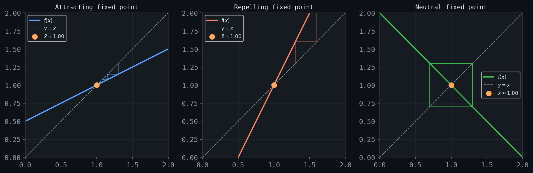Fixed Point Stability Types Figure: The three fixed-point stability cases illustrated via cobweb diagrams. Left: attracting. Centre: repelling. Right: neutral.

For linear maps $f(x) = ax$, we found that $\bar{x} = 0$ is attracting when $|a| < 1$ and repelling when $|a| > 1$. For a nonlinear $f$, the linearization of $f$ at a fixed point $\bar{x}$ is

\[ f(x) \approx L_{\bar{x}}(x) = \bar{x} + f'(\bar{x})(x - \bar{x}), \]

which behaves like the linear map $g(y) = f'(\bar{x}) \cdot y$ in the displaced variable $y = x - \bar{x}$. This suggests that $|f'(\bar{x})|$ plays the role of the multiplier $|a|$.

Theorem (Local Stability Criterion). Let $f \in C^1[a,b]$ and suppose $\bar{x} \in (a,b)$ is a fixed point of $f$.

If $|f'(\bar{x})| < 1$, then $\bar{x}$ is attracting: there exists an open interval $I \ni \bar{x}$ such that $f^n(x) \to \bar{x}$ for all $x \in I$.
If $|f'(\bar{x})| > 1$, then $\bar{x}$ is repelling: for $x \in I \setminus \{\bar{x}\}$, the orbit eventually leaves any neighbourhood of $\bar{x}$.

Proof (attracting case). Since $|f'(\bar{x})| < 1$ and $f'$ is continuous, there exists an open interval $J \ni \bar{x}$ and a constant $0 \leq K < 1$ such that $|f'(x)| \leq K$ for all $x \in J$. Let $I \subset J$ be an open interval centered at $\bar{x}$. For any $x \in I$, the Mean Value Theorem gives a $c$ between $x$ and $\bar{x}$ with \[ |f(x) - \bar{x}| = |f(x) - f(\bar{x})| = |f'(c)| |x - \bar{x}| \leq K|x - \bar{x}|. \] Thus $f(x) \in I$, and repeating the argument: $|f^n(x) - \bar{x}| \leq K^n |x - \bar{x}| \to 0$.

Remark. A companion theorem shows that no other fixed points of $f$ can lie in the interval $I$. If another fixed point $\bar{y} \in I$ existed, the Mean Value Theorem applied to $\bar{x}$ and $\bar{y}$ would require $f'(c) = 1$ for some $c \in I$, contradicting $|f'| \leq K < 1$ on $I$.

Geometric Interpretation and Classification

For a fixed point $\bar{x}$ with $0 < f'(\bar{x}) < 1$: the cobweb converges monotonically — a staircase descending toward $\bar{x}$.

For $-1 < f'(\bar{x}) < 0$: the cobweb converges but oscillates around $\bar{x}$ — a damped spiral.

For $f'(\bar{x}) > 1$: the cobweb diverges monotonically away from $\bar{x}$.

For $f'(\bar{x}) < -1$: the cobweb diverges with oscillations.

For $f'(\bar{x}) = -1$: a neutral fixed point with particularly delicate behaviour — the local dynamics depends on higher-order terms. For example, the map $f_{-1}(x) = -x$ has $\bar{x} = 0$ as neutral, and every point $x_0$ belongs to a two-cycle $(x_0, -x_0)$.

Examples

Example 1: $f(x) = x^2$. Fixed points satisfy $x^2 = x$, giving $\bar{x}_1 = 0$ and $\bar{x}_2 = 1$. Since $f'(x) = 2x$, we get $f'(0) = 0 < 1$ (attracting) and $f'(1) = 2 > 1$ (repelling). Orbits starting in $(-1, 1)$ converge to $0$; orbits starting outside $[-1,1]$ diverge.

Example 2: $f(x) = \sqrt{x}$ for $x \geq 0$. Fixed points: $\bar{x}_1 = 0$ and $\bar{x}_2 = 1$. We have $f'(x) = \frac{1}{2\sqrt{x}}$, so $f'(1) = \frac{1}{2} < 1$ (attracting). At $x = 0$, $f'(0^+) = +\infty > 1$ (repelling), confirming the graphical picture.

Example 3: $f(x) = \cos x$. The fixed point satisfies $\cos \bar{x} = \bar{x}$, giving $\bar{x} \approx 0.7391$ (the Dottie number). Since $|f'(\bar{x})| = |\sin \bar{x}| \approx 0.674 < 1$, this fixed point is globally attracting: for any $x_0 \in \mathbb{R}$, the iterates $x_n \to \bar{x}$.

Chapter 3: The Logistic Map and Bifurcations

Population Dynamics and the Logistic Map

The logistic map $f_a(x) = ax(1-x)$ on $[0,1]$ with parameter $a \in (0,4]$ serves as the central laboratory of this course. It arises from the discrete analogue of the logistic differential equation $\frac{dx}{dt} = ax - bx^2$, after a rescaling that sets the carrying capacity to 1.

The function $f_a$ is a downward-opening parabola with $f_a(0) = f_a(1) = 0$ and a global maximum of $\frac{a}{4}$ at $x = \frac{1}{2}$. For $a \leq 4$, this maximum satisfies $\frac{a}{4} \leq 1$, so $f_a : [0,1] \to [0,1]$.

Fixed Points and Their Stability

The fixed points of $f_a$ satisfy $ax(1-x) = x$, giving:

$\bar{x}_1 = 0$ (always a fixed point),
$\bar{x}_2 = \frac{a-1}{a} = 1 - \frac{1}{a}$ (exists in $(0,1)$ only for $a > 1$).

Computing the derivative: $f_a'(x) = a(1 - 2x)$.

At $\bar{x}_1 = 0$: $f_a'(0) = a$. So $\bar{x}_1$ is attracting for $0 < a < 1$ and repelling for $a > 1$.

At $\bar{x}_2 = \frac{a-1}{a}$: $f_a'(\bar{x}_2) = a\bigl(1 - 2\frac{a-1}{a}\bigr) = a \cdot \frac{2-a}{a} = 2 - a$. Thus $|\bar{x}_2\text{'s multiplier}| = |2-a|$, and:

$\bar{x}_2$ is attracting when $1 < a < 3$ (since $|2-a| < 1$ iff $1 < a < 3$),
$\bar{x}_2$ is neutral when $a = 3$ (since $|2-3| = 1$),
$\bar{x}_2$ is repelling when $a > 3$.

The First Bifurcation at $a = 1$

At $a = 1$: $\bar{x}_2(1) = 0$, coinciding with $\bar{x}_1$. As $a$ increases past 1, the fixed point $\bar{x}_1 = 0$ becomes repelling and $\bar{x}_2 = 1 - 1/a$ enters $(0,1)$ as an attracting fixed point. The two fixed points exchange stability at this transcritical bifurcation.

The Period-Doubling Bifurcation at $a = 3$

The qualitative change at $a = 3$ is more dramatic. As $a \to 3^-$, the derivative at $\bar{x}_2$ approaches $-1$. At precisely $a = 3$, the fixed point is neutral: $f_3'(\bar{x}_2) = -1$. For $a$ slightly greater than 3, the fixed point $\bar{x}_2$ becomes repelling.

What replaces the attracting fixed point? To find out, we study the second iterate $g = f_a^2 = f_a \circ f_a$. The fixed points of $g$ include the fixed points of $f_a$ together with any two-cycles $(p_1, p_2)$ satisfying $f_a(p_1) = p_2$ and $f_a(p_2) = p_1$.

For $a > 3$, the graph of $f_a^2(x)$ develops two new intersection points with $y = x$ on either side of $\bar{x}_2$, giving an attracting two-cycle $(p_1(a), p_2(a))$. Solving $f_a(p_1) = p_2$ and $f_a(p_2) = p_1$ yields (after subtracting the fixed-point equations) that the two-cycle points satisfy the quadratic

\[ x^2 - \frac{a+1}{a}x + \frac{a+1}{a} = 0, \]

giving

\[ p_{1,2} = \frac{1}{2}\left(\frac{a+1}{a} \pm \frac{\sqrt{(a+1)(a-3)}}{a}\right). \]

These are real and distinct precisely when $a > 3$, confirming the bifurcation at (a = 3$.

Stability of the Two-Cycle

The attractivity of the two-cycle $(p_1, p_2)$ is determined by the derivative of $f_a^2$ at either point (by the chain rule they are equal):

\[ (f_a^2)'(p_1) = f_a'(p_2) \cdot f_a'(p_1). \]

This product equals $-1$ when $a = 3$ (as the two-cycle is born) and decreases as $a$ increases. The two-cycle is attracting as long as $|(f_a^2)'(p_1)| < 1$, i.e., for $3 < a < 1 + \sqrt{6} \approx 3.449$.

At $a = 1 + \sqrt{6}$, the two-cycle becomes neutral $(|(f_a^2)'(p_i)| = 1)$, and for larger $a$, it becomes repelling while giving birth to an attracting four-cycle. This is the period-doubling phenomenon.

The Period-Doubling Cascade and Feigenbaum’s Constant

The sequence of bifurcation parameter values continues:

$a_1 = 3$: period 1 → 2 (two-cycle appears),
$a_2 = 1 + \sqrt{6} \approx 3.449$: period 2 → 4,
$a_3 \approx 3.544$: period 4 → 8,
$a_4 \approx 3.5644$: period 8 → 16,
$\vdots$
$a_\infty \approx 3.5699456\ldots$: accumulation point; chaos begins.

The ratios of consecutive gaps $\delta_n = \frac{a_{n+1} - a_n}{a_{n+2} - a_{n+1}}$ converge to the Feigenbaum constant

\[ \delta = \lim_{n \to \infty} \delta_n = 4.6692016\ldots \]

This constant is universal — it appears in the period-doubling cascades of all smooth one-dimensional maps with a single quadratic maximum, a remarkable discovery of Mitchell Feigenbaum (1978).

The Bifurcation Diagram

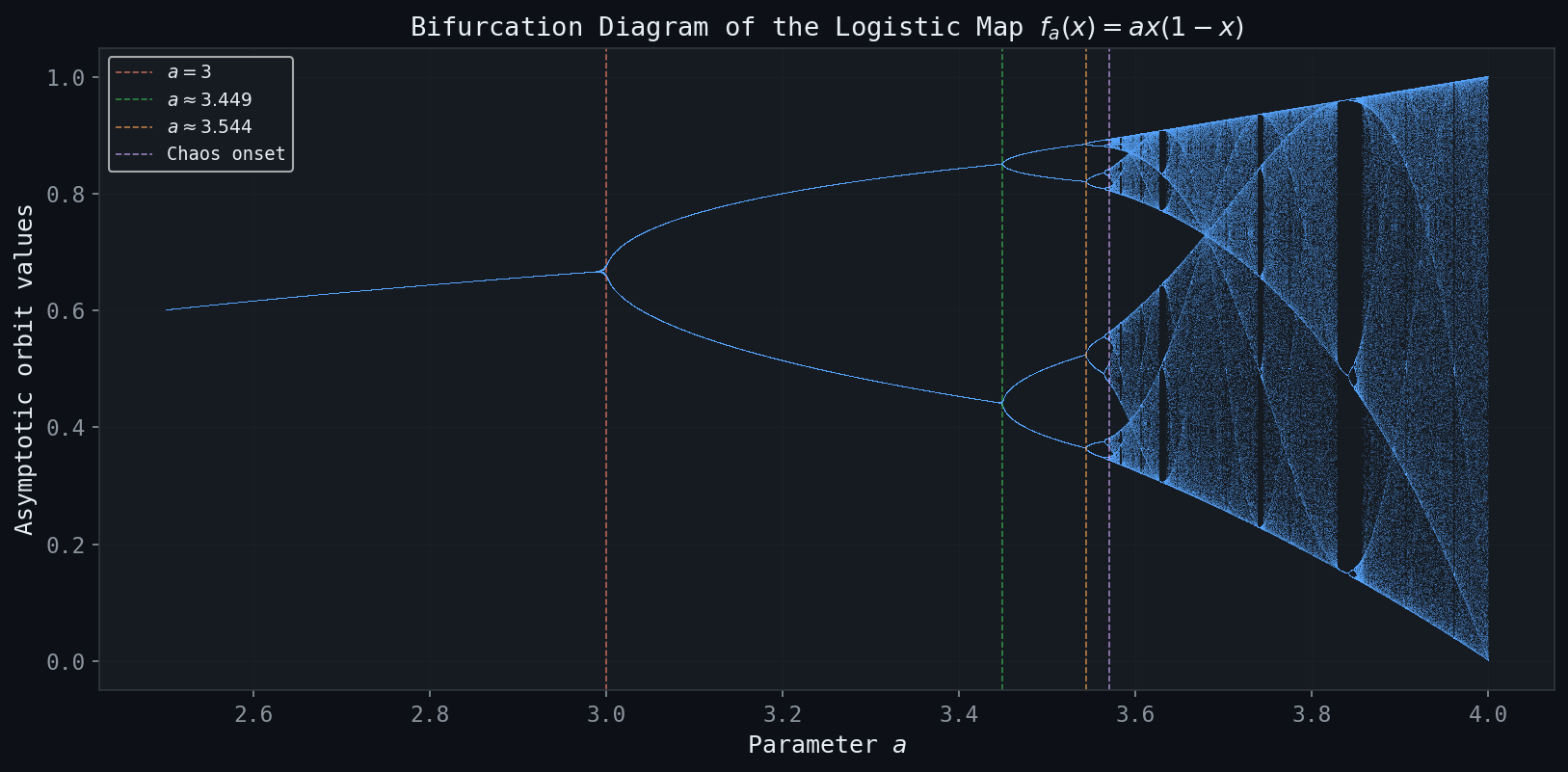Bifurcation Diagram of the Logistic Map Figure: The bifurcation diagram of $f_a(x)$. Period-doubling bifurcations accumulate at the Feigenbaum point $a_\infty \approx 3.5699$.

The bifurcation diagram plots, for each parameter $a$, the long-term iterates of the logistic map (discarding transients). For $1 < a < 3$, the diagram shows a single curve (the attracting fixed point $\bar{x}_2$). At $a = 3$, this curve splits into two (the two-cycle), which in turn split at $a \approx 3.449$, producing a self-similar cascade of period doublings culminating in the chaotic regime for $a > a_\infty$. Within the chaotic regime, there are also windows of periodicity — the most prominent is the period-3 window near $a \approx 3.83$.

The Case $a = 4$: Full Chaos

The logistic map $f_4(x) = 4x(1-x)$ is especially significant. It maps $[0,1]$ onto $[0,1]$ (the maximum value is $4 \cdot \frac{1}{4} = 1$) and is two-to-one (every $y \in (0,1)$ has two preimages). The iterates of $f_4$ from a typical starting point appear random and irregular. This is the prototypical example of chaos, which we will study in depth.

Chapter 4: Periodic Orbits and the Li-Yorke Theorem

Periods and $n$-Cycles

We have seen that for $a > 3$, the logistic map has two-cycles; for $a > 1 + \sqrt{6}$, four-cycles emerge. A natural question is: which periods can coexist? The answer is given by the remarkable theorems of Li-Yorke and Sharkovsky.

Definition. A point $p$ has minimal period $n$ if $f^n(p) = p$ and $f^k(p) \neq p$ for all $0 < k < n$. The orbit $\{p, f(p), \ldots, f^{n-1}(p)\}$ is called a period-$n$ orbit or an $n$-cycle.

Recall that for the logistic map $f_4(x)$, the iterates of $f_4^n$ double in count with each iteration: $f_4^n(x)$ has exactly $2^n$ fixed points, so $f_4$ has $2^n$ periodic points of period $n$ for every $n \geq 1$.

The Li-Yorke Theorem: Period Three Implies Chaos

One of the most celebrated results in discrete dynamical systems is the following theorem, published in the American Mathematical Monthly in 1975.

Theorem (Li-Yorke, 1975). Let $f : J \to J$ be a continuous function on an interval $J$. Suppose there exists a point $a \in J$ such that \[ f^3(a) \leq a < f(a) < f^2(a) \quad \text{or} \quad f^3(a) \geq a > f(a) > f^2(a). \] (That is, $f$ has a point of period 3.) Then:

For every $n \geq 1$, $f$ has a periodic point of period $n$.
There exists an uncountable set $S \subset J$ (containing no periodic points) such that for all $x, y \in S$ with $x \neq y$: \[ \limsup_{n \to \infty} |f^n(x) - f^n(y)| > 0 \quad \text{and} \quad \liminf_{n \to \infty} |f^n(x) - f^n(y)| = 0. \] Furthermore, for every periodic point $p$ and every $x \in S$: \[ \limsup_{n \to \infty} |f^n(x) - f^n(p)| > 0. \]

The uncountable set $S$ in condition (2) is said to exhibit chaos in the sense of Li and Yorke: any two distinct points in $S$ come arbitrarily close at some times yet are bounded apart at other times.

Proof Structure of the Li-Yorke Theorem

The proof proceeds by constructing explicit periodic orbits of each period $n > 3$ using the Intermediate Value Theorem. We sketch the key argument.

Assume WLOG $f(a) = b$, $f(b) = c$, $f(c) = a$ (so $a < b < c$, i.e., $a$ has period 3). Define $I_0 = [a, b]$ and $I_1 = [b, c]$. From the assumption, $f(I_0) \supseteq I_1$ and $f(I_1) \supseteq I_0 \cup I_1$.

To find a period-$n$ point for arbitrary $n \geq 2$:

Step 1. Define nested intervals $J_0 \supseteq J_1 \supseteq \cdots \supseteq J_{n-1}$ by:

Choose $J_0 \subset I_1$ with $f(J_0) = I_0$.
For $k = 1, \ldots, n-2$: choose $J_k \subset J_{k-1}$ with $f^k(J_k) \subset I_1$ (keeping iterates in $I_1$).
At the final step, require $f^{n-1}(J_{n-1}) \supseteq J_0$.

Step 2. By nested compactness, $\bigcap_{k=0}^{n-1} J_k \neq \emptyset$. For any $p$ in this intersection, $f^n(p) = p$ by the construction (applying the Intermediate Value Theorem at each step).

Step 3. Showing minimality: The construction ensures that the first $n-2$ iterates $f^k(p)$ lie in $[b, c]$, the $(n-1)$st iterate $f^{n-1}(p)$ lies in $[a, b)$, and $f^n(p)$ returns to $[b,c]$. No shorter return to the same position is possible, establishing that $p$ genuinely has period $n$.

The Sharkovsky Ordering

The Li-Yorke Theorem is a special case of a broader theorem due to the Ukrainian mathematician A.N. Sharkovsky (1964). Define the Sharkovsky ordering of the positive integers:

\[ 3 \triangleleft 5 \triangleleft 7 \triangleleft \cdots \triangleleft 2 \cdot 3 \triangleleft 2 \cdot 5 \triangleleft \cdots \triangleleft 4 \cdot 3 \triangleleft 4 \cdot 5 \triangleleft \cdots \triangleleft 2^3 \triangleleft 2^2 \triangleleft 2 \triangleleft 1. \]

The ordering places all odd integers first (in increasing order), then all doubles of odd integers, then four times the odd integers, etc., and finally the pure powers of 2 in decreasing order.

Theorem (Sharkovsky, 1964). Let $f : J \to J$ be continuous on an interval. If $f$ has a periodic point of period $m$, then $f$ has periodic points of all periods $n$ with $m \triangleleft n$ in the Sharkovsky ordering.

The Li-Yorke Theorem corresponds to the case $m = 3$, which is the first element in the Sharkovsky ordering — hence period 3 implies all other periods.

Example. For the logistic map with $3.829 \leq a \leq 3.840$, a three-cycle exists. By the Li-Yorke theorem, periodic orbits of every period exist in this parameter range.

Chapter 5: Chaotic Dynamics — Definitions and Lyapunov Exponents

Devaney’s Definition of Chaos

Several inequivalent definitions of chaos exist. The most widely used in the context of this course is due to Robert Devaney.

Definition (Devaney Chaos). A continuous map $f : I \to I$ is said to be chaotic on $I$ if:

Dense periodic points: The set of periodic points of $f$ is dense in $I$.
Topological transitivity: For any two open intervals $U, V \subset I$, there exists an $n \geq 0$ such that $f^n(U) \cap V \neq \emptyset$. Equivalently, there exists a point $x \in I$ whose forward orbit is dense in $I$.
Sensitive dependence to initial conditions (SDIC): There exists $\varepsilon > 0$ such that for any $x \in I$ and any $\delta > 0$, there exists $y \in (x-\delta, x+\delta)$ and $n \geq 0$ with $|f^n(x) - f^n(y)| > \varepsilon$.

Remark. It can be shown (Banks et al., 1992) that conditions (1) and (2) together imply condition (3). So SDIC is in some sense redundant. Nevertheless, it captures the most physically important aspect of chaos: tiny differences in initial conditions are amplified exponentially over time. This is sometimes called the "butterfly effect."

The Tent Map as the Prototype of Chaos

The tent map $T(x)$ is chaotic on $[0,1]$. This follows easily from its piecewise linear nature:

\[ |T(x) - T(y)| = 2|x - y|. \]

After $n$ applications (provided iterates stay on the same piece), $|T^n(x) - T^n(y)| = 2^n |x - y|$. Any initial separation is amplified by a factor of $2^n$, establishing SDIC.

The logistic map $f_4$ is semi-conjugate to the tent map (see Chapter 6), which transfers the chaotic properties of $T$ to $f_4$.

Lyapunov Exponents

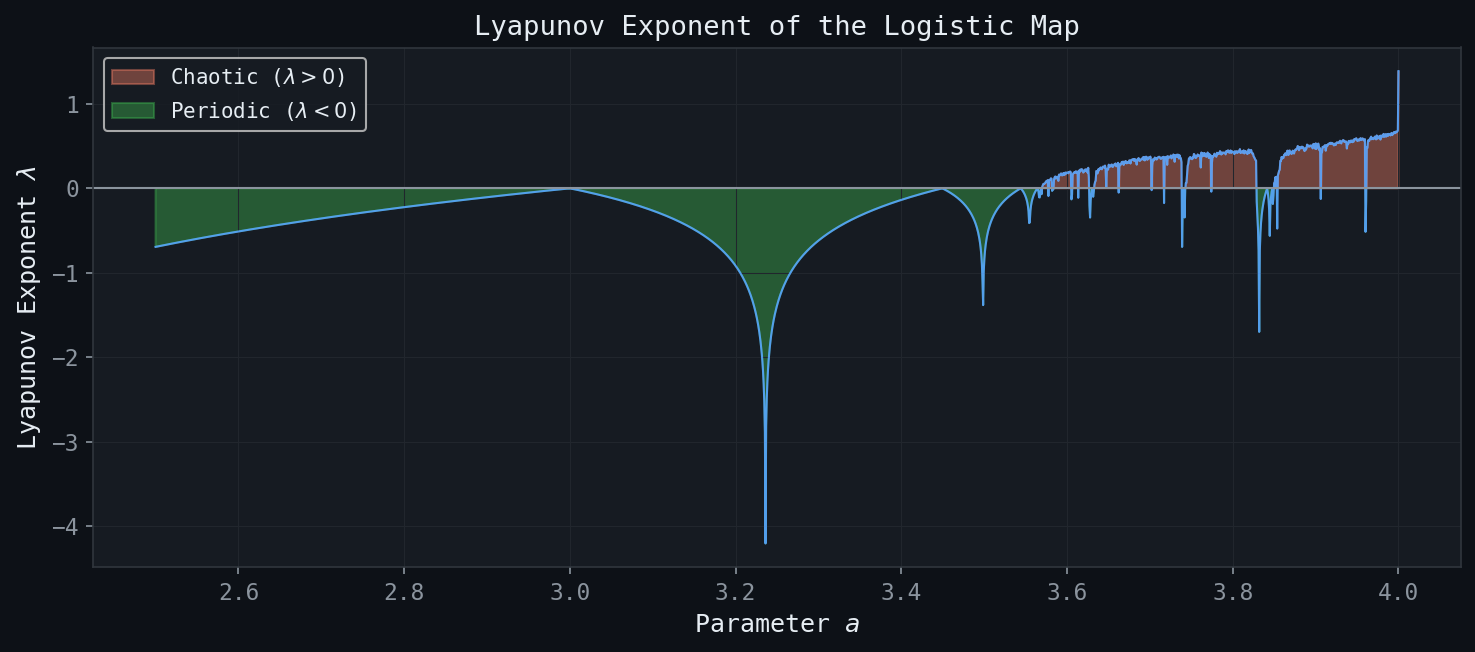Lyapunov Exponent of the Logistic Map Figure: The Lyapunov exponent $\lambda(a)$ of the logistic map. Positive values indicate chaos; deep negative dips correspond to superstable periodic orbits.

The Lyapunov exponent provides a quantitative measure of the rate at which nearby orbits separate under iteration.

Definition (Lyapunov Exponent). For a $C^1$ map $f : I \to I$ and a seed point $x_0 = x$, define the iteration sequence $x_k = f^k(x)$. The Lyapunov exponent of $f$ at $x$ is \[ \lambda(x) = \lim_{n \to \infty} \frac{1}{n} \ln |(f^n)'(x)|, \] provided the limit exists.

The intuition is that nearby orbits separate like $e^{n\lambda(x)}$: a positive $\lambda$ indicates exponential expansion (chaotic behaviour), while a negative $\lambda$ indicates exponential contraction (convergence to an attractor).

Computing the Lyapunov Exponent

By the chain rule applied repeatedly:

\[ (f^n)'(x_0) = \prod_{k=0}^{n-1} f'(x_k). \]

Taking logarithms and averaging:

\[ \lambda(x) = \lim_{n \to \infty} \frac{1}{n} \sum_{k=0}^{n-1} \ln |f'(x_k)|. \]

This is the time average of $\ln |f'|$ along the orbit of $x$.

\[ \lambda = \frac{1}{n} \cdot n \ln 2 = \ln 2 \approx 0.693. \]

The positive Lyapunov exponent confirms that the tent map is expansive and chaotic.

Lyapunov Exponents for Attracting Fixed Points

Theorem. If $\bar{x}$ is an attracting fixed point of $f \in C^1(I)$ and $x_0 \in W(\bar{x})$ (the basin of attraction), then \[ \lambda(x_0) = \ln |f'(\bar{x})| < 0. \]

The proof uses the fact that the orbit $\{x_k\}$ converges to $\bar{x}$, so for large $k$, $\ln|f'(x_k)|$ is close to $\ln|f'(\bar{x})|$. A careful $\varepsilon$-$N$ argument then shows the Cesàro average converges to $\ln|f'(\bar{x})|$.

Lyapunov Exponents for the Logistic Map

The derivative of $f_a$ is $f_a'(x) = a(1-2x)$. For $f_4(x) = 4x(1-x)$:

\[ f_4'(x) = 4(1-2x). \]

The Lyapunov exponent can be computed analytically using the invariant measure of $f_4$ (Chapter 7):

\[ \lambda = \int_0^1 \ln|4(1-2x)| \cdot \rho(x)\, dx = \ln 2, \]

where $\rho(x) = \frac{1}{\pi\sqrt{x(1-x)}}$ is the arcsine density. Remarkably, the Lyapunov exponent of $f_4$ equals that of the tent map — a consequence of their conjugacy.

For $0 < a \leq 3$, when iterates converge to the fixed point $\bar{x}_2 = 1 - 1/a$, we have $\lambda = \ln|2-a|$. The Lyapunov exponent is negative (contracting) for $1 < a < 3$ and equals $-\infty$ at $a = 2$ (where $f_2'(\bar{x}_2) = 0$).

For $3 < a < 1 + \sqrt{6}$, when iterates converge to a two-cycle $(p_1, p_2)$:

\[ \lambda = \frac{1}{2}\bigl(\ln|f_a'(p_1)| + \ln|f_a'(p_2)|\bigr) = \frac{1}{2}\ln|(f_a^2)'(p_1)|. \]

Lyapunov Exponents and Numerical Computation

SDIC has important practical consequences. Since any numerical computation introduces rounding errors of order $\varepsilon \approx 10^{-16}$ (double precision), after $n$ steps the error in the orbit is approximately $\varepsilon e^{n\lambda}$. When $\lambda \approx \ln 2$, an error of $10^{-16}$ grows to $O(1)$ after about $\frac{16 \ln 10}{\ln 2} \approx 53$ iterations. As Devaney noted: “the results of numerical computation of an orbit, no matter how accurate, may bear no resemblance whatsoever with the real orbit.”

Chapter 6: Symbolic Dynamics

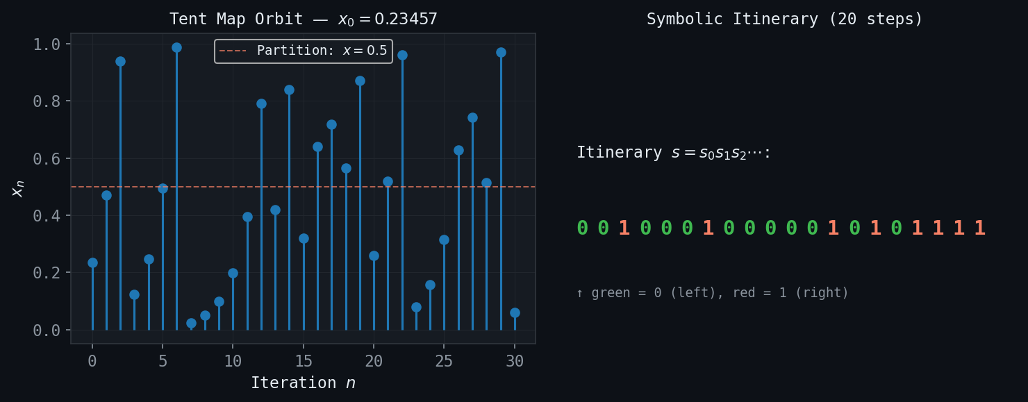Symbolic Dynamics: Tent Map Orbit and Itinerary Figure: A tent map orbit (left) and its symbolic itinerary encoded as a binary sequence (right). The shift map acts on these sequences.

The Core Idea

Symbolic dynamics replaces the study of orbits of a map $f : I \to I$ with the study of sequences over a finite alphabet. Instead of tracking the precise numerical value of $f^n(x)$, we record only which region (labelled $0$ or $1$) each iterate falls in. This coarse description turns out to contain all the essential dynamical information.

The Baker Map and Binary Expansions

The Baker map (or doubling map) is

\[ B(x) = 2x \bmod 1 = \begin{cases} 2x, & 0 \leq x < \tfrac{1}{2}, \\ 2x - 1, & \tfrac{1}{2} \leq x < 1. \end{cases} \]

Every $x \in [0,1]$ has a binary expansion $x = \sum_{k=0}^{\infty} b_k / 2^{k+1}$, written $x = .b_0 b_1 b_2 \ldots$ with $b_k \in \{0,1\}$. The action of $B$ is simply a left shift:

\[ B(x) = .b_1 b_2 b_3 \ldots \]

The first binary digit $b_0$ is “consumed” (thrown away), and the decimal point shifts one place to the right. This is the Bernoulli shift map $S : \Sigma_2 \to \Sigma_2$ on the space of binary sequences

\[ \Sigma_2 = \{(b_0, b_1, b_2, \ldots) \mid b_k \in \{0,1\}\}. \]

The metric on $\Sigma_2$ is $d_{\Sigma_2}(b, b') = \sum_{k=0}^{\infty} \frac{|b_k - b_k'|}{2^k}$. Two sequences are close iff their first many digits agree.

Symbolic Dynamics for the Baker Map

Fixed points of $B$: The sequences $(0,0,0,\ldots)$ and $(1,1,1,\ldots)$ are fixed by $S$, corresponding to $x = 0$ and $x = 1$.

Two-cycles: The sequences $(0,1,0,1,\ldots)$ and $(1,0,1,0,\ldots)$ form a two-cycle of $S$. The corresponding points in $[0,1]$ are $p_1 = \frac{1}{3}$ and $p_2 = \frac{2}{3}$ (geometric series).

Period-$n$ orbits: Any repeating sequence of period $n$, e.g., $(b_0 b_1 \cdots b_{n-1} b_0 b_1 \cdots)$, is a period-$n$ point of $S$. There are exactly $2^n$ such sequences of period $n$, one in each dyadic subinterval of length $2^{-n}$. As $n \to \infty$, these periodic points fill $[0,1]$ densely.

Using Symbolic Dynamics to Prove Chaos

SDIC for $B$: Given any $x : b = (b_0, b_1, \ldots)$ and any $\delta > 0$, choose $N$ so large that $2^{-N} < \delta$. Define $y : b' = (b_0, \ldots, b_{N-1}, \overline{b_N}, \ldots)$, agreeing with $b$ to $N$ digits but differing at position $N$. Then $|x - y| \leq 2^{-N} < \delta$. After \(N$ applications of $B$, the first digit of $B^N(x)$ is $b_N$ while the first digit of $B^N(y)$ is $\overline{b_N} \neq b_N$. Hence $B^N(x)$ and $B^N(y)$ lie in different half-intervals, separated by at least $\frac{1}{2}$. This proves SDIC with $\varepsilon = \frac{1}{4}$.

Density of periodic orbits: For any $x \in [0,1]$ and any neighbourhood $(x - \delta, x + \delta)$, choose $N$ so that $2^{-N} < \delta$. The repeating sequence $(b_0, b_1, \ldots, b_{N-1}, b_0, b_1, \ldots)$ defines a periodic point $p$ of period $N$ which satisfies $|x - p| \leq 2^{-N} < \delta$.

\[ x = .0 \;|\; 00 \; 01 \; 10 \; 11 \;|\; 000 \; 001 \; 010 \; \cdots \]

The orbit $\{B^n(x)\}_{n \geq 0}$ is dense in $[0,1]$, since after a left-shift by $m$ steps, the leading digits of $B^m(x)$ can be made to match any prescribed binary sequence of length $N$, placing $B^m(x)$ within $2^{-N}$ of any target point.

Itinerary Sequences for the Tent Map

For the tent map $T$, we define the itinerary of $x \in [0,1]$ by

\[ b_k = \begin{cases} 0 & \text{if } T^k(x) \in [0, \tfrac{1}{2}], \\ 1 & \text{if } T^k(x) \in (\tfrac{1}{2}, 1]. \end{cases} \]

This produces a binary sequence $b = (b_0, b_1, b_2, \ldots)$. The tent map’s action on itineraries is not a simple left-shift (because the second piece is decreasing), but there is a modified version: if the current digit is 0, the next digit is unchanged; if 1, all subsequent digits are flipped. This defines a shift with flipping, which is topologically conjugate to the standard Bernoulli shift.

The key conclusion: knowing that the Bernoulli shift $S$ is chaotic (SDIC, dense periodic orbits, transitivity) allows us to conclude, via the correspondence $x \leftrightarrow b = b(x)$, that the tent map $T$ is also chaotic on $[0,1]$.

Symbolic Dynamics for the Logistic Map $f_4$

The logistic map $f_4(x) = 4x(1-x)$ is semi-conjugate to the tent map $T$ via the substitution $x = \sin^2(\pi t / 2)$. More precisely, defining $\phi : [0,1] \to [0,1]$ by $\phi(t) = \sin^2(\pi t / 2)$, one verifies that

\[ f_4(\phi(t)) = \phi(T(t)). \]

This semi-conjugacy transfers all chaotic properties (SDIC, transitivity, density of periodic points) from $T$ to $f_4$. In terms of itinerary sequences, $f_4$ and $T$ assign the same binary sequence to any pair $(x, t)$ with $x = \phi(t)$.

The Cantor-Like Invariant Set of $f_a$ for $a > 4$

When $a > 4$, the maximum of $f_a$ exceeds 1, so $f_a$ maps some points outside $[0,1]$. Define

\[ \Lambda = \{x \in [0,1] : f_a^n(x) \in [0,1] \text{ for all } n \geq 0\}. \]

This invariant set is a Cantor-like set. Points not in $\Lambda$ escape to $-\infty$ under iteration. The symbolic dynamics on $\Lambda$ is again given by a shift on $\Sigma_2$, where $b_k = 0$ if $f_a^k(x) \in I_0$ and $b_k = 1$ if $f_a^k(x) \in I_1$ (the two pre-image intervals). This gives a complete description of the chaotic dynamics restricted to $\Lambda$.

Chapter 7: Invariant Measures and Spatial Distribution of Orbits

Visitation Frequencies and Histograms

When a map $f : I \to I$ is chaotic, the orbit of a typical point $x_0$ is dense on $I$. But how are the iterates distributed? To answer this, we construct a histogram: divide $I = [0,1]$ into $N$ equal subintervals $J_k = [(k-1)/N, k/N)$, compute a long orbit $\{x_n\}_{n=1}^{M}$, and let $c_k$ be the number of iterates falling in $J_k$. The normalized histogram is $p_k = c_k / M$.

For the tent map: the histogram is approximately flat — each subinterval is visited with equal frequency $p_k \approx 1/N$. This is consistent with the tent map’s linearity and uniform spreading of points.

For the logistic map $f_4$: the histogram is markedly non-uniform — visits cluster near $x = 0$ and $x = 1$, with fewer visits near $x = \frac{1}{2}$. The distribution curves up at both endpoints.

These empirical observations call for a mathematical framework.

The Invariant Density Function

As $N, M \to \infty$, we expect the histogram to converge to a continuous density function $\rho(x)$. The fraction of orbit time spent in $[a,b] \subset [0,1]$ is

\[ F([a,b]) = \int_a^b \rho(x)\, dx, \]

normalized so that $\int_0^1 \rho(x)\, dx = 1$. The conservation principle underlying the density is:

Definition (Invariant Measure). A probability density $\rho : I \to [0,\infty)$ is invariant for $f : I \to I$ if for all measurable $S \subset I$, \[ \int_S \rho(x)\, dx = \int_{f^{-1}(S)} \rho(x)\, dx, \] where $f^{-1}(S) = \{x : f(x) \in S\}$. Equivalently, defining the measure $\mu(S) = \int_S \rho\, dx$, \[ \mu(S) = \mu(f^{-1}(S)) \quad \text{for all } S. \]

The condition says: the measure of a set $S$ equals the measure of all points that map into $S$ — a conservation of measure under the dynamics, analogous to conservation of mass in fluid mechanics.

The Invariant Density for the Tent Map

Claim: $\rho(x) = 1$ (the uniform distribution) is invariant for the tent map $T$.

Verification: For any $[a,b] \subset [0,1]$, the preimage $T^{-1}([a,b])$ consists of two subintervals, each of length $\frac{b-a}{2}$, since $|T'(x)| = 2$ everywhere. Thus

\[ \int_{T^{-1}([a,b])} 1\, dx = 2 \cdot \frac{b-a}{2} = b - a = \int_a^b 1\, dx. \]

The invariance holds. The uniform distribution is the absolutely continuous invariant measure (ACIM) of the tent map.

The Invariant Density for the Logistic Map $f_4$

For $f_4(x) = 4x(1-x)$, the invariant density is the arcsine distribution:

\[ \rho(x) = \frac{1}{\pi \sqrt{x(1-x)}}, \qquad x \in (0,1). \]

This density diverges at both endpoints $x = 0$ and $x = 1$, explaining the clustering of orbits near the boundaries.

Derivation. The semi-conjugacy $f_4 \circ \phi = \phi \circ T$, where $\phi(t) = \sin^2(\pi t/2)$, implies that the invariant measure of $f_4$ is the pushforward of the uniform measure on $[0,1]$ (for $T$) through $\phi$. For $y = \phi(t)$, the change of variables $dt = \frac{dt}{dy} dy = \frac{1}{\phi'(t)} dy$ gives the density:

\[ \rho(y) = \frac{1}{|\phi'(\phi^{-1}(y))|}= \frac{1}{\pi \sqrt{y(1-y)}}. \]

Verification: For $[a,b] \subset [0,1]$, $f_4^{-1}([a,b]) = [a_1, b_1] \cup [a_2, b_2]$ where $f_4$ has two branches. Transforming the integral using both branches and the substitution $u = 4x(1-x)$ confirms the invariance condition.

Physical and Statistical Interpretation

The invariant density $\rho$ describes the time-average distribution of the chaotic orbit. More precisely, the ergodic theorem (Birkhoff, 1931) states that for a.e. $x_0$ (with respect to $\rho$),

\[ \lim_{M \to \infty} \frac{1}{M} \sum_{n=0}^{M-1} g(f^n(x_0)) = \int_I g(x) \rho(x)\, dx \]

for any continuous function $g$. Thus, computing long-orbit averages of $g$ is equivalent to integrating $g$ against $\rho$.

This means the Lyapunov exponent of $f_4$ can be computed as:

\[ \lambda = \int_0^1 \ln |f_4'(x)| \rho(x)\, dx = \int_0^1 \ln|4(1-2x)| \frac{dx}{\pi\sqrt{x(1-x)}} = \ln 2. \]

Chapter 8: Cantor Sets and Fractal Topology

The Ternary Cantor Set: Construction

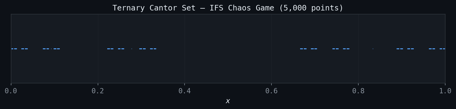Cantor Set via IFS Chaos Game Figure: The ternary Cantor set generated by 5,000 random IFS iterations. The self-similar gap structure is clearly visible.

The ternary Cantor set $C$ is constructed from the unit interval $[0,1]$ by a recursive middle-thirds deletion process:

Stage 0: $C_0 = [0,1]$.
Stage 1: Remove the open middle third: $C_1 = [0,\tfrac{1}{3}] \cup [\tfrac{2}{3},1]$.
Stage 2: Remove the open middle thirds of each remaining interval: $C_2 = [0,\tfrac{1}{9}] \cup [\tfrac{2}{9},\tfrac{1}{3}] \cup [\tfrac{2}{3},\tfrac{7}{9}] \cup [\tfrac{8}{9},1]$.
Stage $n$: $C_n$ is a union of $2^n$ closed intervals each of length $3^{-n}$.
Limit: $C = \bigcap_{n=0}^{\infty} C_n.$

Properties of the Cantor Set

The Cantor set exhibits a remarkable combination of properties that seem contradictory:

Property 1: $C$ is closed. As an intersection of closed sets, $C$ is closed.

Property 2: $C$ is uncountable. Every $x \in C$ has a ternary expansion using only digits $\{0, 2\}$ (never $1$). The mapping $t_k \in \{0,2\} \mapsto b_k = t_k/2 \in \{0,1\}$ provides a bijection between $C$ and all binary sequences, hence between $C$ and $[0,1]$. Since $[0,1]$ is uncountable, so is $C$. In fact, $|C| = |\mathbb{R}| = \aleph_1$.

\[ \frac{1}{3} + \frac{2}{9} + \frac{4}{27} + \cdots = \sum_{k=0}^{\infty} \frac{2^k}{3^{k+1}} = \frac{1/3}{1 - 2/3} = 1. \]

Alternatively, $L(C_n) = (2/3)^n \to 0$.

Property 4: $C$ is perfect. Every point of $C$ is a limit point of $C$ (equivalently, $C$ contains no isolated points). This follows because both endpoints of every removed interval belong to $C$ and accumulate on each other.

Property 5: $C$ is nowhere dense. No open interval is contained in $C$; every neighbourhood of a point in $C$ contains points not in $C$ (the removed intervals).

Property 6: $C$ is totally disconnected. The connected components of $C$ are single points — the maximum connected subsets are singletons.

Countability, Uncountability, and Transfinite Cardinals

The surprising uncountability of $C$ motivates a brief discussion of infinity. Recall:

A set is countable if its elements can be listed in a sequence $a_1, a_2, a_3, \ldots$. Examples: $\mathbb{N}$, $\mathbb{Z}$, $\mathbb{Q}$. The cardinality of countably infinite sets is $\aleph_0$.
A set is uncountable if no such listing is possible. Examples: $\mathbb{R}$, $[0,1]$, the Cantor set $C$. Cardinality $\aleph_1 = 2^{\aleph_0}$.

Cantor’s diagonal argument (1891) shows $\mathbb{R}$ is uncountable: if all reals in $[0,1]$ were listed $r_1, r_2, r_3, \ldots$, construct a number $d$ differing from $r_n$ in the $n$th decimal digit — then $d$ is not in the list, a contradiction.

Ternary Representation and the Cantor Set

Every $x \in [0,1]$ has a ternary (base-3) expansion $x = \sum_{k=0}^{\infty} t_k / 3^{k+1}$ with $t_k \in \{0,1,2\}$. The key observation is:

The Cantor set consists precisely of those $x \in [0,1]$ whose ternary expansion uses only the digits $0$ and $2$.

This is because removing the middle third $(\frac{1}{3}, \frac{2}{3})$ removes all $x$ with $t_0 = 1$. Removing the middle thirds of the remaining intervals removes those with $t_1 = 1$, and so on. The Cantor set consists of ternary expansions with no digit equal to 1.

Cantor-Like Sets and the Invariant Set of $f_a$ for $a > 4$

A Cantor-like set is any set homeomorphic to the ternary Cantor set — perfect, compact, totally disconnected, and uncountable. Such sets arise naturally in dynamics. For instance, the invariant set

\[ \Lambda_a = \{x \in [0,1] : f_a^n(x) \in [0,1] \text{ for all } n \geq 0\} \]

of the logistic map with $a > 4$ is a Cantor-like set. Its construction mirrors that of the ternary Cantor set: at each stage, points whose iterate falls outside $[0,1]$ are removed, leaving two subintervals. The process produces a Cantor-like set of fractal dimension $\log 2 / \log(a/(a-4))$ (for large $a$, this approaches $\log 2 / \log a$ and decreases toward 0 as $a \to \infty$).

The Tent Map and the Cantor Set

Consider the modified tent map (with slope 3)

\[ T_3(x) = \begin{cases} 3x, & 0 \leq x \leq \tfrac{1}{3}, \\ 3 - 3x, & \tfrac{2}{3} \leq x \leq 1, \\ \text{(outside } [0,1] \text{ for } x \in (\tfrac{1}{3}, \tfrac{2}{3})), \end{cases} \]

extended so that $T_3$ maps the middle third outside $[0,1]$. The set of points that remain in $[0,1]$ for all iterations is exactly the ternary Cantor set $C$. The map $T_3 : C \to C$ is well-defined and the itinerary sequences (labelling each iterate as in $I_0 = [0,\frac{1}{3}]$ or $I_1 = [\frac{2}{3}, 1]$) provide a bijective coding of the Cantor set dynamics by the Bernoulli shift.

Chapter 9: Two-Dimensional Nonlinear Dynamics

Maps in $\mathbb{R}^2$

We now extend the iteration framework to two dimensions. A discrete dynamical system in $\mathbb{R}^2$ is given by a map $f : \mathbb{R}^2 \to \mathbb{R}^2$:

\[ \mathbf{x}_{n+1} = f(\mathbf{x}_n), \qquad \mathbf{x}_n = (x_n, y_n) \in \mathbb{R}^2. \]

Writing $f(\mathbf{x}) = (f_1(x,y), f_2(x,y))$, a fixed point $\bar{\mathbf{x}} = (\bar{x}, \bar{y})$ satisfies $f(\bar{\mathbf{x}}) = \bar{\mathbf{x}}$, i.e., the system of equations $f_1(\bar{x},\bar{y}) = \bar{x}$ and $f_2(\bar{x},\bar{y}) = \bar{y}$.

Linearization and the Jacobian Matrix

Near a fixed point $\bar{\mathbf{x}}$, the behaviour of the nonlinear system is approximated by its linearization. Setting $\mathbf{u}_n = \mathbf{x}_n - \bar{\mathbf{x}}$ (displacement from the fixed point):

\[ \mathbf{u}_{n+1} \approx A \mathbf{u}_n, \qquad A = Df(\bar{\mathbf{x}}) = J_f(\bar{\mathbf{x}}), \]

where $A$ is the Jacobian matrix of $f$ evaluated at the fixed point:

\[ A = \begin{pmatrix} \frac{\partial f_1}{\partial x} & \frac{\partial f_1}{\partial y} \\[6pt] \frac{\partial f_2}{\partial x} & \frac{\partial f_2}{\partial y} \end{pmatrix}_{\bar{\mathbf{x}}}. \]

The local behaviour of the nonlinear system near $\bar{\mathbf{x}}$ is governed by the eigenvalues $\lambda_1, \lambda_2$ of $A$.

Classification of Fixed Points by Eigenvalues

Theorem. Let $f : \mathbb{R}^2 \to \mathbb{R}^2$ with fixed point $\bar{\mathbf{x}}$, and let $\lambda_1, \lambda_2$ be the eigenvalues of the Jacobian $Df(\bar{\mathbf{x}})$.

Attracting (stable) node or spiral: If $|\lambda_1| < 1$ and $|\lambda_2| < 1$, the fixed point is locally attracting.
Repelling (unstable) node or spiral: If $|\lambda_1| > 1$ and $|\lambda_2| > 1$, the fixed point is locally repelling.
Saddle point: If $|\lambda_1| < 1 < |\lambda_2|$ (or vice versa), the fixed point is a saddle: attracting along one eigenspace, repelling along the other.
Centre (neutral): If $|\lambda_1| = |\lambda_2| = 1$, the behaviour is indeterminate from the linearization alone.

When the eigenvalues are complex conjugates $\lambda = re^{\pm i\theta}$ with $r = |\lambda|$, the orbit spirals: inward ($r < 1$), outward ($r > 1$), or on a circle ($r = 1$).

A Worked Example

Consider the map $f : \mathbb{R}^2 \to \mathbb{R}^2$ defined by

\[ f(x,y) = \left(\frac{1}{2}(x^2 + y^2),\; xy\right). \]

Finding fixed points: The fixed-point equations $\frac{1}{2}(x^2+y^2) = x$ and $xy = y$ give four solutions: $\mathbf{x}_1 = (0,0)$, $\mathbf{x}_2 = (2,0)$, $\mathbf{x}_3 = (1,-1)$, $\mathbf{x}_4 = (1,1)$.

Jacobian matrix:

\[ A(x,y) = \begin{pmatrix} x & y \\ y & x \end{pmatrix}. \]

At $\mathbf{x}_1 = (0,0)$: $A = \begin{pmatrix} 0 & 0 \\ 0 & 0 \end{pmatrix}$, eigenvalues $\lambda_1 = \lambda_2 = 0$. Fixed point is attracting (superattracting).

At $\mathbf{x}_2 = (2,0)$: $A = \begin{pmatrix} 2 & 0 \\ 0 & 2 \end{pmatrix}$, eigenvalues $\lambda_1 = \lambda_2 = 2 > 1$. Fixed point is repelling.

At $\mathbf{x}_3 = (1,-1)$: $A = \begin{pmatrix} 1 & -1 \\ -1 & 1 \end{pmatrix}$, eigenvalues $\lambda_1 = 2, \lambda_2 = 0$. Fixed point is a saddle: attracting along eigenvector $(1,1)$, repelling along $(1,-1)$.

At $\mathbf{x}_4 = (1,1)$: Similarly a saddle, with eigenvalues $\lambda_1 = 2, \lambda_2 = 0$, attracting along $(1,-1)$, repelling along $(1,1)$.

The basin of attraction of $(0,0)$ turns out to be the diamond-shaped region $\{(x,y) : |x| + |y| < 2\}$, bounded by the invariant lines of the saddle fixed points.

Invariant Lines

In the above example, the line $y = 2 - x$ is invariant under $f$. To verify: any point $(x, 2-x)$ maps to $\left(x^2 - 2x + 2,\; 2x - x^2\right)$, and $(2x - x^2) = 2 - (x^2 - 2x + 2)$, so the image lies on the same line. This invariance explains the diamond structure of the basins.

Chapter 10: Complex Dynamics and Julia Sets

Iteration of Polynomials in $\mathbb{C}$

We now move to the complex plane $\mathbb{C} \cong \mathbb{R}^2$. The iteration of complex polynomials reveals fractal structures of extraordinary beauty and mathematical depth. The simplest nontrivial family is the complex quadratic family:

\[ g_c(z) = z^2 + c, \qquad z \in \mathbb{C}, \quad c \in \mathbb{C}. \]

For $c = 0$, this reduces to $g_0(z) = z^2\, whose dynamics we can analyze completely: \(|g_0^n(z)| = |z|^{2^n}$, so $|z| < 1$ leads to $0$, $|z| > 1$ leads to $\infty$, and $|z| = 1$ is invariant.

Fixed Points of $g_c$

The fixed points of $g_c$ satisfy $z^2 + c = z$, or $z^2 - z + c = 0$, giving:

\[ z_{1,2} = \frac{1 \pm \sqrt{1-4c}}{2}. \]

For $c \neq \frac{1}{4}$, there are two distinct fixed points.

Theorem. For $c \neq \frac{1}{4}$, at least one fixed point of $g_c$ is repelling.

Proof. The derivatives at the fixed points are $g_c'(z_{1,2}) = 2z_{1,2} = 1 \pm \sqrt{1-4c} = 1 \pm w$ where $w = \sqrt{1-4c} \neq 0$. The two values $1+w$ and $1-w$ are symmetric about 1. Since $w \neq 0$, at least one of $|1+w|$ or $|1-w|$ exceeds 1 — specifically, the one on the far side of $|z|=1$ from the other. Hence at least one fixed point is repelling.

The Filled Julia Set and the Julia Set

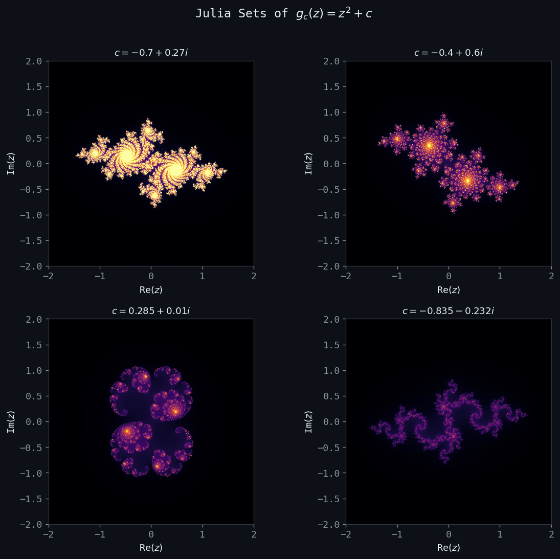Julia Sets of gc(z) = z² + c Figure: Julia sets for four values of $c$. The structure changes dramatically as $c$ moves inside and outside the Mandelbrot set.

Definition. The filled Julia set (or prisoner set) of $g_c$ is \[ K_c = \{z \in \mathbb{C} : g_c^n(z) \not\to \infty\} = \{z : \text{the orbit of } z \text{ is bounded}\}. \] The Julia set $J_c$ is the boundary of $K_c$: \[ J_c = \partial K_c. \]

Equivalently, the Julia set $J_c$ is the closure of the set of all repelling periodic points of $g_c$. The complement $\mathbb{C} \setminus K_c$ is the escaping set — orbits starting there diverge to $\infty$.

Theorem (Boundedness of $J_c$). If $|z| > |c| + 1$, then $|g_c^n(z)| \to \infty$. Consequently, $J_c \subset \{|z| \leq |c|+1\}$.

Proof. For $|z| > |c| + 1$, using the reverse triangle inequality: \[ |g_c(z)| = |z^2 + c| \geq |z|^2 - |c| = |z|(|z| - |c|/|z|). \] Since $|z| > |c| + 1 > 1$, we can show $|g_c(z)| > r|z|$ for some $r > 1$, so $|g_c^n(z)| > r^n |z| \to \infty$.

Invariance of the Julia Set

Theorem. $J_c$ is invariant under $g_c$: $g_c(J_c) = J_c$.

This means the Julia set is a fractal attractor for the inverse map. If $z \in J_c$, then $g_c(z) \in J_c$. Moreover, any preimage $g_c^{-1}(z)$ of a point $z \in J_c$ also lies in $J_c$.

Structure of Julia Sets: Examples

$c = 0$: $J_0 = \{|z| = 1\}$, the unit circle. This is a smooth closed curve.

$c$ real, $-3/4 < c < 1/4$: The Julia set is a connected closed curve (Jordan curve) that becomes increasingly “crinkly” as $c$ moves away from 0. These are fractal curves with dimension $> 1$.

$c = -3/4$: The fixed point $z_1 = \frac{1}{2}$ becomes indifferent ($|g_c'(z_1)| = 1$) and becomes part of $J_c$.

$c = -2$: $J_{-2} = [-2, 2] \subset \mathbb{R}$. The real quadratic map $f_{-2}(x) = x^2 - 2$ is chaotic on $[-2,2]$ with Lyapunov exponent $\ln 2$.

$c < -2$ (real): $J_c$ is a Cantor set on the real line. Orbits escape from the interval.

$c > 1/4$ (real): $J_c$ is totally disconnected.

$c = i$: $J_i$ is a dendrite-like connected set.

The Connectivity Dichotomy

A fundamental theorem (Douady-Hubbard, 1982) characterizes when $J_c$ is connected:

Theorem. The Julia set $J_c$ is connected if and only if the orbit of the critical point $z = 0$ under $g_c$ is bounded, i.e., $0 \in K_c$. If the orbit of 0 escapes to $\infty$, then $J_c$ is a Cantor set (totally disconnected).

This theorem reduces the question of connectivity to the behaviour of a single orbit — that of the critical point $z = 0$ (the unique point with $g_c'(0) = 0$).

The Mandelbrot Set

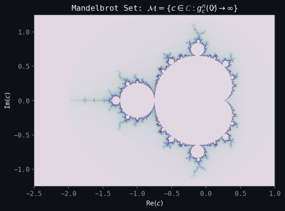Figure: The Mandelbrot set $\mathcal{M}$. Points colored by escape speed; black points belong to $\mathcal{M}$.

The Mandelbrot set $\mathcal{M}$ encodes the connectivity of Julia sets as a function of the parameter $c$:

\[ \mathcal{M} = \{c \in \mathbb{C} : g_c^n(0) \not\to \infty\} = \{c \in \mathbb{C} : J_c \text{ is connected}\}. \]

By the boundedness theorem, if $|c| > 2$ then $c \notin \mathcal{M}$ (since $g_c(0) = c$ and $|c| > 2$ implies the orbit escapes). So $\mathcal{M} \subset \{|c| \leq 2\}$.

The Mandelbrot set is connected (Douady-Hubbard), has fractal boundary with Hausdorff dimension 2 (Shishikura, 1998), and contains infinitely many “baby Mandelbrot sets” embedded in its boundary. The bulbs of $\mathcal{M}$ correspond to parameter values for which $g_c$ has an attracting periodic orbit: the main cardioid corresponds to an attracting fixed point, the period-2 bulb to an attracting two-cycle, etc. In fact, the combinatorial structure of the Mandelbrot set encodes all the bifurcations of the logistic map.

The Escaping Set and the Green’s Function

For $c \in \mathcal{M}$ (i.e., $c \notin \mathcal{M}$), one can define the escape time of $z$ as the smallest $n$ with $|g_c^n(z)| > R$ (for large $R$). The escape time colouring — assigning colours based on how quickly orbits escape — produces the familiar rainbow images of the Mandelbrot set boundary.

Chapter 11: Fractal Dimension

Measuring “Size” with Box-Counting Dimension

Classical sets in $\mathbb{R}^n$ have integer dimensions: a point has dimension 0, a curve has dimension 1, a surface has dimension 2, a solid region has dimension 3. Fractal sets require a more flexible concept.

The box-counting dimension (or Minkowski dimension) is defined as follows. For a bounded set $A \subset \mathbb{R}^k$, let $N(\varepsilon)$ denote the minimum number of balls (or cubes) of diameter $\varepsilon$ needed to cover $A$.

Definition (Box-Counting Dimension). The box-counting dimension of $A$ is \[ D = \lim_{\varepsilon \to 0} \frac{\ln N(\varepsilon)}{\ln(1/\varepsilon)}, \] provided the limit exists.

The scaling relation that underlies this definition is $N(\varepsilon) \sim C \varepsilon^{-D}$ for small $\varepsilon$. Equivalently, if we rescale by a factor $r < 1$:

\[ N(r\varepsilon) = N(\varepsilon) \cdot r^{-D}. \]

Self-Similar Fractals: $D = \ln N / \ln(1/r)$

For a self-similar fractal $A$ that is the union of $N$ copies of itself, each scaled by a factor $r$, the scaling relation gives immediately:

\[ N(r\varepsilon) = N \cdot N(\varepsilon) \quad \Rightarrow \quad r^{-D} = N \quad \Rightarrow \quad D = \frac{\ln N}{\ln(1/r)}. \]

Example 1: The Ternary Cantor Set. $C$ consists of $N = 2$ copies of itself, each scaled by $r = 1/3$. Thus \[ D = \frac{\ln 2}{\ln 3} \approx 0.631. \] This is consistent with $C$ being "larger" than a finite point set (dimension 0) but "smaller" than an interval (dimension 1): it is a fractional dimension between 0 and 1.

Example 2: The Sierpinski Triangle. The Sierpinski triangle $S$ is the union of $N = 3$ contracted copies, each with scale factor $r = 1/2$: \[ D = \frac{\ln 3}{\ln 2} \approx 1.585. \] Since $1 < D < 2$, the Sierpinski triangle is "thicker" than a one-dimensional curve but "thinner" than a two-dimensional region. The scaling argument: shrinking the triangle by $1/2$ in both directions gives a piece that is one-third the original — not one-half (as for a line) nor one-quarter (as for an area). This anomalous scaling is the hallmark of fractality.

The Von Koch Curve

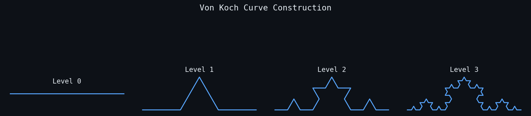Von Koch Curve Construction Figure: Von Koch curve at levels 0, 1, 2, and 3. The limiting curve has infinite length and fractal dimension $\ln 4/\ln 3 \approx 1.262$.

The von Koch curve $C_K$ is constructed by repeatedly replacing the middle third of each line segment with an equilateral bump:

Generator: A segment of length $l$ is replaced by 4 segments of length $l/3$.
Limiting curve: $C_K = \lim_{n\to\infty} C_n$, where $C_0 = [0,1]$ and each $C_{n+1} = G(C_n)$.

Properties:

$C_K$ is self-similar: it consists of $N = 4$ copies scaled by $r = 1/3$.
Fractal dimension: $D = \frac{\ln 4}{\ln 3} \approx 1.261$.
$C_K$ has infinite length (length $L_n = (4/3)^n \to \infty$) but zero area.
$C_K$ is continuous everywhere but differentiable nowhere.

The von Koch snowflake is formed by applying the von Koch generator to all three sides of an equilateral triangle. It has finite area but infinite perimeter — a striking paradox that captures the essence of fractal geometry.

Generalized Von Koch Curves

Replacing the middle third with a bump consisting of $n$ segments each of length $rl$ gives a generalized von Koch curve with dimension

\[ D(n, r) = \frac{\ln n}{\ln(1/r)}, \qquad \frac{1}{n} \leq r \leq \frac{1}{2}. \]

For inhomogeneous scaling with contraction ratios $r_1, \ldots, r_n$, the dimension is the unique solution $D$ to the Moran equation:

\[ \sum_{i=1}^{n} r_i^D = 1. \]

Additional Examples

\[ D = \frac{\ln 8}{\ln 3} = \frac{3\ln 2}{\ln 3} \approx 1.893. \]\[ D = \frac{\ln 20}{\ln 3} \approx 2.727. \]\[ D = \frac{\ln 4}{\ln 2} = 2. \]

A counterintuitive result: the 3D Sierpinski gasket, a fractal living in $\mathbb{R}^3$, has the same fractal dimension as a planar surface — because its “holes” make it scale as a 2D object.

Hausdorff Dimension

The Hausdorff dimension is a more mathematically rigorous notion that agrees with the box-counting dimension for most natural fractals but is better-behaved theoretically. For a set $A \subset \mathbb{R}^k$, define the $d$-dimensional Hausdorff measure:

\[ \mathcal{H}^d(A) = \lim_{\varepsilon \to 0} \inf\left\{ \sum_i |U_i|^d : A \subset \bigcup_i U_i, |U_i| \leq \varepsilon \right\}. \]

There exists a critical value $D_H$ such that $\mathcal{H}^d(A) = \infty$ for $d < D_H$ and $\mathcal{H}^d(A) = 0$ for $d > D_H$. This critical value is the Hausdorff dimension of $A$.

For the Cantor set, $D_H = \frac{\ln 2}{\ln 3}$; for the Sierpinski triangle, $D_H = \frac{\ln 3}{\ln 2}$. For smooth curves, $D_H = 1$; for smooth surfaces, $D_H = 2$. For the boundary of the Mandelbrot set, $D_H = 2$.

Fractals in Nature

Benoit Mandelbrot (1924-2010) coined the term “fractal” (from the Latin fractus, meaning broken or fragmented) in his 1977 book Fractals: Form, Chance and Dimension. He documented fractal structures throughout nature:

Coastlines, mountain ranges, river networks.
Trees, ferns, bronchial tubes, blood vessels.
Clouds, snowflakes, lightning bolts.
Galaxy clusters.

The ubiquity of fractals in nature suggests that self-similarity and fractal dimension are fundamental features of how natural processes operate — growth, branching, turbulence, and roughness all generate fractal geometry.

Chapter 12: Iterated Function Systems

Contraction Mappings and Banach’s Theorem

The mathematical foundation of iterated function systems rests on the theory of contraction mappings in complete metric spaces.

Definition (Metric Space). A metric space $(X, d)$ consists of a set $X$ and a distance function $d : X \times X \to [0,\infty)$ satisfying:

Positivity: $d(x,y) \geq 0$, with $d(x,y) = 0 \iff x = y$.
Symmetry: $d(x,y) = d(y,x)$.
Triangle inequality: $d(x,z) \leq d(x,y) + d(y,z)$ for all $x,y,z \in X$.

Definition (Cauchy Sequence and Completeness). A sequence $\{x_n\} \subset X$ is a Cauchy sequence if for every $\varepsilon > 0$ there exists $N_\varepsilon$ such that $d(x_m, x_n) < \varepsilon$ for all $m, n > N_\varepsilon$. The metric space $(X,d)$ is complete if every Cauchy sequence converges to an element of $X$.

Key examples: $(\mathbb{R}^n, d_2)$ (Euclidean distance) is complete. The rational numbers $\mathbb{Q}$ with $d(x,y) = |x-y|$ are not complete (Cauchy sequences may converge to irrationals).

Definition (Contraction Mapping). A map $f : X \to X$ on a metric space $(X,d)$ is a contraction mapping (or contraction) if there exists a constant $c_f \in [0,1)$ such that \[ d(f(x), f(y)) \leq c_f \cdot d(x,y) \quad \text{for all } x, y \in X. \] The constant $c_f$ is called the contraction factor (or Lipschitz constant) of $f$.

Theorem (Banach Fixed Point Theorem, 1922). Let $(X, d)$ be a complete metric space and $f : X \to X$ a contraction mapping with contraction factor $c_f \in [0,1)$. Then:

There exists a unique fixed point $\bar{x} \in X$ with $f(\bar{x}) = \bar{x}$.
For any $x_0 \in X$, the iteration sequence $x_{n+1} = f(x_n)$ converges to $\bar{x}$.
The following error estimate holds: \[ d(x_n, \bar{x}) \leq \frac{c_f^n}{1-c_f} d(x_0, x_1). \]

Proof sketch. Starting from any $x_0$, the triangle inequality applied repeatedly gives \[ d(x_m, x_n) \leq \left(c_f^m + c_f^{m+1} + \cdots + c_f^{n-1}\right) d(x_0, x_1) \leq \frac{c_f^m}{1-c_f} d(x_0, x_1). \] Since $c_f < 1$, the right side $\to 0$ as $m \to \infty$, so $\{x_n\}$ is Cauchy. By completeness, $x_n \to \bar{x} \in X$. Continuity of $f$ (which follows from the contraction property) gives $f(\bar{x}) = \bar{x}$. Uniqueness: if $\bar{y} = f(\bar{y})$, then $d(\bar{x}, \bar{y}) = d(f(\bar{x}), f(\bar{y})) \leq c_f d(\bar{x}, \bar{y})$, forcing $d(\bar{x}, \bar{y}) = 0$, so $\bar{x} = \bar{y}$.

Iterated Function Systems: Definition

Definition (IFS). An iterated function system (IFS) is a collection $\mathcal{F} = \{f_1, f_2, \ldots, f_N\}$ of $N \geq 2$ contraction mappings on a closed bounded subset $D \subset \mathbb{R}^n$, i.e., for each $k$, $f_k : D \to D$ with contraction factor $c_k \in [0,1)$.

The IFS acts not on individual points but on sets. For any set $S \subset D$, define the Hutchinson operator $\hat{f}$ by:

\[ \hat{f}(S) = \bigcup_{k=1}^{N} f_k(S). \]

The Hausdorff Metric

To apply Banach’s theorem, we need $\hat{f}$ to act as a contraction on a complete metric space of sets. The relevant space is $\mathcal{H}(D)$, the set of all nonempty compact subsets of $D$, equipped with the Hausdorff metric:

\[ h(A, B) = \max\left(\max_{x \in A} d(x, B),\; \max_{y \in B} d(y, A)\right), \]

where $d(x, B) = \min_{y \in B} d(x, y)$. Informally, $h(A,B)$ is the smallest $\varepsilon > 0$ such that $A$ lies in an $\varepsilon$-neighbourhood of $B$ and $B$ lies in an $\varepsilon$-neighbourhood of $A$.

Theorem (Hutchinson, 1981). The metric space $(\mathcal{H}(D), h)$ is complete. Moreover, the Hutchinson operator $\hat{f}$ associated with an IFS $\mathcal{F} = \{f_1, \ldots, f_N\}$ is itself a contraction on $(\mathcal{H}(D), h)$: \[ h(\hat{f}(A), \hat{f}(B)) \leq c \cdot h(A, B), \qquad c = \max_{1 \leq k \leq N} c_k < 1. \]

The Attractor of an IFS

By Banach’s Fixed Point Theorem applied to $\hat{f}$ on the complete metric space $(\mathcal{H}(D), h)$:

Theorem (Existence and Uniqueness of IFS Attractor). There exists a unique nonempty compact set $A \subset D$ satisfying \[ A = \hat{f}(A) = \bigcup_{k=1}^{N} f_k(A). \] Moreover, for any initial set $S_0 \in \mathcal{H}(D)$, the iteration $S_{n+1} = \hat{f}(S_n)$ satisfies $\lim_{n\to\infty} h(S_n, A) = 0$. The set $A$ is called the attractor of the IFS.

The attractor $A$ is self-similar by construction: it is the union of $N$ contracted copies of itself. This is the mathematical foundation of the statement “fractals are self-similar objects.”

Classical Examples of IFS Attractors

Example 1: Ternary Cantor Set. Consider the two-map IFS on $[0,1]$: \[ f_1(x) = \frac{x}{3}, \qquad f_2(x) = \frac{x}{3} + \frac{2}{3}. \] The attractor is the ternary Cantor set $C$. Indeed, $C = f_1(C) \cup f_2(C)$: $C$ is two contracted copies of itself, each scaled by $1/3$, placed at the left and right thirds.

Example 2: Sierpinski Triangle. Consider the three-map IFS in $\mathbb{R}^2$: \[ w_1(x,y) = \left(\frac{x}{2}, \frac{y}{2}\right), \quad w_2(x,y) = \left(\frac{x}{2} + \frac{1}{2}, \frac{y}{2}\right), \quad w_3(x,y) = \left(\frac{x}{2} + \frac{1}{4}, \frac{y}{2} + \frac{\sqrt{3}}{4}\right). \] The attractor is the Sierpinski triangle $S$. Each map shrinks the triangle by factor $1/2$ and translates it to one of the three corners.

Example 3: Barnsley's Fern. A four-map IFS in $\mathbb{R}^2$ using affine maps produces the Barnsley fern, a strikingly realistic leaf shape. The maps model the self-similar structure of a fern: the whole frond contains a scaled copy of itself, each large branch contains smaller copies, etc.

The Random Iteration Algorithm (Chaos Game)

The attractor of an IFS can be approximated by the random iteration algorithm (also called the chaos game, introduced by Barnsley):

Choose an initial point $x_0 \in D$.
At each step $n$, randomly choose one of the maps $f_{k_n}$ (each with probability $p_{k_n} > 0$, $\sum p_k = 1$).
Set $x_{n+1} = f_{k_n}(x_n)$.
After discarding the first few iterates (to allow convergence), plot the orbit $\{x_n\}$.

The resulting point cloud approximates the IFS attractor $A$. The convergence is guaranteed by the theory of iterated function systems with probabilities (IFSP): the orbit visits each part of the attractor with relative frequency proportional to the assigned probabilities, converging to the invariant measure of the IFSP.

Concretely, for the Sierpinski triangle with equal probabilities $p_1 = p_2 = p_3 = 1/3$, the chaos game rapidly fills in the fractal with thousands of points. The probabilities can be chosen to weight the attractor differently; unequal probabilities emphasize different parts and produce a nonuniform fractal measure.

Affine IFS and Fractal Image Compression

An affine IFS uses affine contraction maps of the form $f_k(\mathbf{x}) = A_k \mathbf{x} + \mathbf{b}_k$, where $A_k$ is a matrix with $\|A_k\| < 1$ and $\mathbf{b}_k \in \mathbb{R}^n$. These are the most practically important class of IFS because:

They can produce a wide variety of attractor shapes (ferns, trees, coastlines, etc.) with very compact descriptions (just the matrices $A_k$ and vectors $\mathbf{b}_k$).
The inverse problem (finding an IFS that approximates a given set) can be addressed by the Collage Theorem.

Theorem (Collage Theorem, Barnsley-Ervin-Hardin-Lancaster, 1985). Let $(X, d)$ be a complete metric space and $\hat{f}$ a contraction on $(\mathcal{H}(X), h)$ with contraction factor $c < 1$ and attractor $A$. Then for any set $S \in \mathcal{H}(X)$, \[ h(S, A) \leq \frac{1}{1-c} h(S, \hat{f}(S)). \]

The Collage Theorem says: to approximate a target set $S$ by the attractor $A$ of an IFS, it suffices to find an IFS $\hat{f}$ such that $\hat{f}(S)$ is close to $S$. In other words, make $S$ look like a “collage” of shrunken copies of itself.

Fractal Image Compression

The Collage Theorem provides the theoretical basis for fractal image compression (Barnsley-Sloan, 1988; Jacquin, 1992). The key idea: a digital image (greyscale or colour) can be viewed as a function $u : [0,1]^2 \to \mathbb{R}$ (pixel intensities). An IFSM (Iterated Function System with greyscale Maps) is a system of maps that acts on functions:

\[ (Tu)(x) = \sum_{i=1}^{N} \phi_i(u(w_i^{-1}(x))), \]

where $w_i : [0,1]^2 \to [0,1]^2$ are spatial contractions and $\phi_i : \mathbb{R} \to \mathbb{R}$ are greyscale transformations (typically affine: $\phi_i(t) = \alpha_i t + \beta_i$).

If $T$ is contractive in an appropriate function space, then it has a unique fixed-point function $\bar{u} = T\bar{u}$, the fractal image. The encoding process finds contraction maps $w_i, \phi_i$ such that $T(u) \approx u$ (collage approximation); decoding iterates $T$ from any starting image to recover (\bar{u} \approx u$.

Properties of fractal image compression:

Very high compression ratios possible (the attractor of a small IFS can describe a complex image).
Decoding is fast (iteration of a contraction).
Encoding is computationally expensive (finding the IFS).
Resolution-independent: the attractor can be decoded at any resolution.

The theoretical framework for this can be extended to probability measures (IFSP) and multimeasures, providing a rich mathematical setting for function and image approximation via the fixed points of generalized fractal transforms.

These notes cover PMATH 370: Chaos and Fractals as lectured by Prof. E.R. Vrscay, University of Waterloo, Winter 2020. The material draws on lectures 1–34 and the 2016 Fractal Geometry Seminar on generalized fractal transforms and fractal image compression.