Lecture 1: Introduction

The Probability Space

Random graph theory sits at the intersection of combinatorics and probability, asking: what does a “typical” large graph look like? To make this precise, we work inside a probability space, denoted by the triple \((\mathcal{G}, \mathcal{P}, \mathcal{F})\) where \(\mathcal{G}\) is a class of graphs, \(\mathcal{P}\) is a probability measure, and \(\mathcal{F}\) is a sigma-algebra. In practice, \(\mathcal{G}\) is finite, \(\mathcal{P}\) is a discrete probability measure, and \(\mathcal{F} = 2^{\mathcal{G}}\) is the full power set.

A discrete probability space consists of a countable set \(\Omega\) and a probability function \(P : \Omega \to [0,1]\) with \(\sum_{\omega \in \Omega} P(\omega) = 1\). A subset of \(\Omega\) is an event, with probability \(P(A) = \sum_{\omega \in A} P(\omega)\). A random variable is a function \(X : \Omega \to \mathbb{R}\) with expectation \(E(X) = \sum_{\omega \in \Omega} X(\omega) P(\omega)\).

\[ P\!\left(\bigcup_{i=1}^n A_i\right) = \sum_i P(A_i) - \sum_{i_1 < i_2} P(A_{i_1} \cap A_{i_2}) + \cdots + (-1)^{n-1} P\!\left(\bigcap_{i=1}^n A_i\right). \]

The Union Bound (Boole’s inequality) is the convenient weakening \(P\!\left(\bigcup A_i\right) \leq \sum P(A_i)\). Two events are independent if \(P(A \cap B) = P(A)P(B)\). Linearity of expectation states \(E(X + Y) = E(X) + E(Y)\) for any two random variables, with no independence assumption required.

The Erdős–Rényi Models

The two central models in this course are both due to Erdős and Rényi.

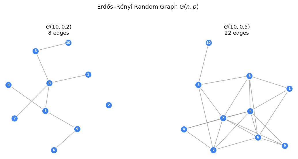
• \(G(n,p)\): a graph on vertex set \([n] = \{1, \ldots, n\}\) is constructed by including each of the \(\binom{n}{2}\) possible edges independently with probability \(p\).
• \(G(n,m)\): a graph is chosen uniformly at random from all graphs on \([n]\) with exactly \(m\) edges.

One can think of \(G(n,m)\) as labelling the edges of \(K_n\) with a random permutation and taking the first \(m\). Other models exist: the random \(d\)-regular graph \(G(n,d)\), the random graph with prescribed degree sequence \(G(n,\tilde{d})\), the random geometric graph \(G(n,r)\) on \(n\) points in the unit square with edges at distance \(\leq r\), and random labelled trees (one of \(n^{n-2}\) trees by Cayley’s formula). This course focuses primarily on the Erdős–Rényi model.

Asymptotic Notation and a.a.s

Given a sequence of probability spaces \((\Omega_n, P_n)_{n \geq 1}\), we say an event \(A_n\) holds asymptotically almost surely (a.a.s) if \(P_n(A_n) \to 1\) as \(n \to \infty\). This is the standard mode of convergence throughout random graph theory.

Useful Estimates

\[ \binom{n}{k} \sim \frac{n^k}{k!}. \]

More precisely, \frac{n^k}{k!} \leq \left(\frac{en}{k}\right)^k. Stirling’s formula gives \(n! = \sqrt{2\pi n}\,(n/e)^n(1 + O(n^{-1}))\), and the inequality \(e^t \geq 1 + t\) holds for all \(t \in \mathbb{R}\).

---

Lecture 2: Concentration Inequalities, Coupling, and the Connection Theorem

Concentration Inequalities

The two classical one-sided and two-sided tail bounds are fundamental throughout.

\[ \Pr(X \geq t) \leq \frac{E[X]}{t}. \]

Proof: let \(I_t = \mathbf{1}[X \geq t]\); then \(X \geq t \cdot I_t\), so taking expectations gives \(E[X] \geq t \cdot P(X \geq t)\).

\[ P(|X - E[X]| \geq t) \leq \frac{\text{Var}(X)}{t^2}. \]\[ P\!\left(|X - Np| \geq f_n\sqrt{p(1-p)N}\right) \leq \frac{1}{f_n^2} = o(1). \]

Coupling

A coupling of two random variables \(X, Y\) is a joint distribution \((\hat{X}, \hat{Y})\) on the same probability space such that marginally \(\hat{X} \sim X\) and \(\hat{Y} \sim Y\).

Coupling Lemma: (a) For \(0 \leq p_1 < p_2 \leq 1\) and \(0 \leq m_1 < m_2 \leq N\), there exist couplings such that \(G(n,p_1) \subseteq G(n,p_2)\) and \(G(n,m_1) \subseteq G(n,m_2)\) always. For the \(p\)-model: start from \(G_1 \sim G(n,p_1)\) and add each non-edge of \(G_1\) independently with probability \(q = 1 - (1-p_2)/(1-p_1)\); then \(G_2 \sim G(n,p_2)\) and \(G_1 \subseteq G_2\) always.

(b) Let \(m_1 = pN - f\sqrt{p(1-p)N}\) and \(m_2 = pN + f\sqrt{p(1-p)N}\). There exists a coupling \((G_1, H, G_2)\) with \(G_1 \sim G(n,m_1)\), \(H \sim G(n,p)\), \(G_2 \sim G(n,m_2)\), and \(P(G_1 \subseteq H \subseteq G_2) = 1 - o(1)\).

A graph property \(Q\) is monotone increasing if \(G \in Q\) and \(H \supseteq G\) implies \(H \in Q\). It is convex if \(G_1, G_2 \in Q\) and \(G_1 \subseteq G_2\) implies \(H \in Q\) for all \(G_1 \subseteq H \subseteq G_2\).

For monotone properties, coupling implies: if \(p_1 \leq p_2\), then \(P(G(n,p_1) \in Q) \leq P(G(n,p_2) \in Q)\), and similarly for the \(m\)-model.

The Connection Theorem

The connection theorem allows us to transfer results between the \(G(n,p)\) and \(G(n,m)\) models.

Theorem 2.4 (Connection Theorem): Let \(Q\) be a graph property.

(i) Given \(p = p(n)\). If for all \(m = pN + O(\sqrt{p(1-p)N})\) we have \(G(n,m) \in Q\) a.a.s, then a.a.s \(G(n,p) \in Q\).

(ii) If \(Q\) is convex and \(G(n, m/N) \in Q\) a.a.s, then a.a.s \(G(n,m) \in Q\).

Proof sketch: Part (i) writes \(P(G(n,p) \in Q)\) via the law of total probability, conditioning on the edge count \(m\). Proposition 2.1 says all but an \(o(1)\)-fraction of the probability mass lies within \(f_n\) standard deviations of the mean. Part (ii) conditions on edge count and uses convexity with the coupling to transfer between models.

---

Lecture 3: Thresholds and First-Order Logic

Threshold Functions

\[ P(G(n,p) \in Q) \to \begin{cases} 0 & \text{if } p \ll p_0 \\ 1 & \text{if } p \gg p_0. \end{cases} \]\[ P(G(n,p) \in Q) \to \begin{cases} 0 & \text{if } p \leq (1-\varepsilon)p_0 \\ 1 & \text{if } p \geq (1+\varepsilon)p_0. \end{cases} \]

The window of a threshold is \(\delta(\varepsilon) = p_{1-\varepsilon} - p_\varepsilon\). Bollobás and Thomason (1987) proved that every non-trivial monotone property has a threshold.

First-Order Logic and the 0–1 Law

\[ \forall x\, \forall y\, \exists z\; (x = y \;\vee\; x \sim y \;\vee\; (x \sim z \wedge y \sim z)). \]

Fix \(k > 0\) and let \(P_k\) be the extension property: for any disjoint sets \(W, V \subseteq V(G)\) of order at most \(k\), there exists a vertex \(x \notin W \cup V\) adjacent to every vertex in \(W\) and to none in \(V\).

Lemma 3.1: If \(m(n)\) and \(p(n)\) satisfy \(mn^{-2+\varepsilon} \to \infty\) and \((N-m)n^{-2+\varepsilon} \to \infty\) (resp. \(pn^\varepsilon \to \infty\) and \((1-p)n^\varepsilon \to \infty\) for every fixed \(\varepsilon > 0\), then a.a.s \(G(n,p) \in P_k\) and \(G(n,m) \in P_k\).

Theorem 3.2 (0–1 Law, first-order logic): Under the conditions of Lemma 3.1, every graph property expressible by a first-order sentence either holds a.a.s or fails a.a.s. Proof sketch: the argument uses an Ehrenfeucht–Fraïssé game. Player 1 picks vertices from either graph; Player 2 responds from the other graph. After \(k\) rounds, Player 2 wins if the map \(v_i \mapsto v_i'\) is an isomorphism between the induced subgraphs. Two graphs sharing the same theory \(\mathrm{Th}_k\) (first-order sentences of quantifier depth \(\leq k\) are indistinguishable by Player 2.

---

Lecture 4: Small Subgraphs and Theorem E

Cycles and Small Subgraphs

Lemma 4.1: If \(p = o(1/n)\), then a.a.s \(G(n,p)\) has no cycles. Proof: Markov’s inequality applied to the expected cycle count.

\[ E[Y_k] = \binom{n}{k} \cdot \frac{(k-1)!}{2} \cdot p^k \sim \frac{n^k}{k!} \cdot \frac{(k-1)!}{2} \cdot \frac{c^k}{n^k} = \frac{c^k}{2k}. \]

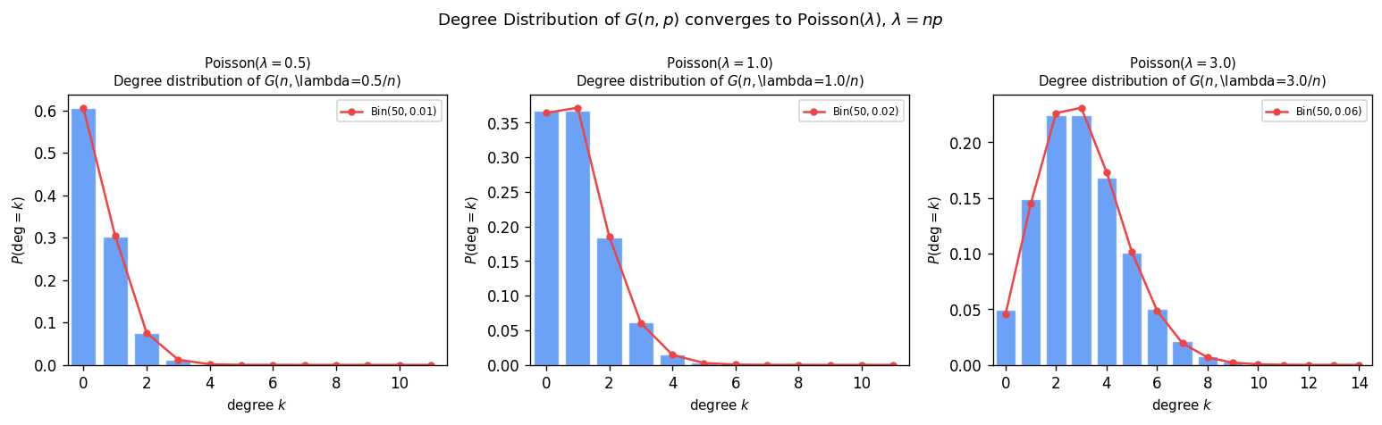
Theorem 5.2: For \(p = c/n\) with \(c > 0\) fixed, \(Y_k \to \mathrm{Po}(c^k/(2k))\) as \(n \to \infty\).

The convergence to a Poisson distribution uses the method of moments: a sequence \((X_n)\) converges to \(\mathrm{Po}(\lambda)\) if and only if all factorial moments satisfy \(E[(X_n)_r] \to \lambda^r\) for all \(r \geq 0\) (where \((x)_r = x(x-1)\cdots(x-r+1)\). For the proof, one counts ordered lists of \(r\) vertex-disjoint \(k\)-cycles (the dominant contribution) and shows the vertex-intersecting cases contribute \(o(1)\).

Theorem E: The Evolution of Random Graphs

The following theorem, which we call Theorem E, describes how the component structure of \(G(n,p)\) evolves as \(p\) increases from 0 to 1. It is one of the central results of the theory.

Theorem E (Erdős–Rényi, Bollobás–Łuczak):

(a) Fix \(k \geq 2\). If \(n^{(k-2)/(k-1)} \ll p \ll n^{(k-1)/k - 2}\)… [forest regime with max component order \(k\)].

(b) If \(p \ll 1/n\), then a.a.s \(G(n,p)\) is a forest and the largest component has order \(o(\log n)\).

(c) If \(p = c/n\) with \(0 < c < 1\), then a.a.s every component of \(G(n,p)\) is a tree or unicyclic, and the largest component has order \(\Theta(\log n)\).

(d) If \(p = c/n\) with \(c > 1\), then a.a.s \(G(n,p)\) contains a unique giant component of linear order, and all other components have order \(O(\log n)\).

(e) When \(p \geq (\log n + \log\log n + \omega(1))/n\), a.a.s \(G(n,p)\) has a giant component and only finitely many isolated vertices.

(f) When \(p \geq (\log n + \omega(1))/n\), a.a.s \(G(n,p)\) is connected and has a perfect matching (if \(n\) is even) or a near-perfect matching.

(g) When \(p \geq (\log n + \log\log n + \omega(1))/n\), a.a.s \(G(n,p)\) is Hamiltonian.

Proof of (a): The forest statement follows from the cycle count computation above. To show the largest component has order exactly \(k\), let \(X_t\) be the number of trees of order \(t\) in \(G(n,p)\). Show \(E\!\left[\sum_{t \geq k+1} X_t\right] = o(1)\) and apply Markov’s inequality. Then show existence of a tree of order \(k\) by the second moment method.

---

Lecture 5: Degree Distribution and the Critical Window

Degree Distribution

Let \(X\) be the number of isolated vertices in \(G(n,p)\).

Theorem 5.3: Let \(p = c\log n / n\) with \(c > 0\) fixed.

• If \(c < 1\), then a.a.s there exist isolated vertices.
• If \(c > 1\), then a.a.s there are no isolated vertices.

\[ P(G(n,p) \text{ is connected}) \to e^{-e^{-c}}. \]

Proof sketch: Let \(X\) count isolated vertices. Then \(E[X] = n(1-p)^{n-1} \sim ne^{-pn} = e^{-c}\) and the Poisson convergence \(X \to \mathrm{Po}(e^{-c})\) gives \(P(X = 0) \to e^{-e^{-c}}\). One shows that connectedness fails a.a.s if and only if there are isolated vertices (the probability of more complex small components is negligible at this edge density).

The Critical Window

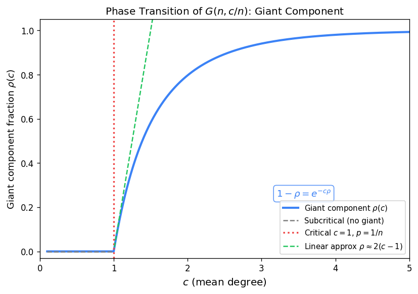
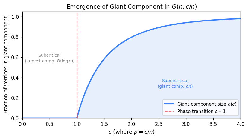
The critical window is the regime \(p = (1 + \varepsilon)/n\) for \(\varepsilon = \varepsilon(n) \to 0\) with \(|\varepsilon|^3 n \to \infty\). This is where the phase transition of Theorem E(d) actually occurs — near \(p = 1/n\), the graph passes from the subcritical regime (many small tree components) to the supercritical regime (a unique giant component).

In the subcritical regime \(c < 1\), the largest component has order \(\Theta(\log n)\). In the supercritical regime \(c > 1\), the giant component has order \(\rho n + o(n)\) where \(\rho = \rho(c)\) is the survival probability of a \(\mathrm{Po}(c)\) Galton–Watson branching process (the unique solution in \((0,1)\) of \(1 - \rho = e^{-c\rho}\).

---

Lecture 6: Bipartite Random Graphs and Perfect Matchings

(Jan 20)

Bipartite Random Graphs

The bipartite random graph \(G(n,n,p)\) has two vertex classes of size \(n\) each, with every cross-edge included independently with probability \(p\).

Exercise: Let \(p = (\log n + c)/n\). Let \(X\) count isolated vertices (vertices of degree 0). Then \(E[X] = 2n(1-p)^n \sim 2e^{-c}\) and \(P(G(n,n,p) \text{ has no isolated vertices}) \to e^{-2e^{-c}}\).

A cherry is a path of length 2 (one vertex of degree 2, two of degree 1). Cherries can be analyzed similarly via the method of moments.

Hall’s Theorem and Perfect Matchings

A perfect matching in \(G(n,n,p)\) is a set of \(n\) vertex-disjoint edges covering all vertices. Hall’s Theorem: a bipartite graph with parts \(A\), \(B\) has a perfect matching if and only if for every \(S \subseteq A\), \(|N(S)| \geq |S|\).

When Hall’s condition fails, there is a set \(S \subseteq A\) such that \(|N(S)| < |S|\). Analyzing such sets: if \(|S| = k\), then the \(k\) vertices of \(S\) must have all their neighbours in a set of size at most \(k-1\). The proof of the perfect matching threshold uses three structural cases on the obstruction set.

Key Lemma: For \((3/4)\log n / n < p < 2\log n / n\), \(\sum_{k} E[X_k] = o(1)\) where \(X_k\) counts the bad sets of size \(k\).

Theorem: \(P(G(n,n,p) \text{ has a perfect matching}) \to e^{-2e^{-c}}\) when \(p = (\log n + c)/n\). The threshold coincides with the disappearance of isolated vertices, just as in the non-bipartite case.

Tree Components in \(G(n,p)\)

\[ E[T_k] \sim \frac{k^{k-2}}{k!}(ce^{-c})^k \cdot n \]\[ t(c) = \frac{1}{c}\sum_{k \geq 1} \frac{k^{k-1}}{k!}(ce^{-c})^k. \]

This function \(t(c)\) connects to the survival probability: for \(c > 1\), the fraction of vertices in finite components is \(1 - \rho(c)\).

---

Lecture 7: Galton–Watson Branching Processes and Chernoff Bounds

(Feb 3)

Threshold Functions: Formal Definition

\[ \lim_{n \to \infty} P(G(n,p) \in Q) = \begin{cases} 0 & p \leq (1-\varepsilon)p_0(n) \\ 1 & p \geq (1+\varepsilon)p_0(n). \end{cases} \]

Recall Theorem E(d): when \(p = c/n\) with \(c > 1\), the fraction of vertices in the giant component is a.a.s \(\rho + o(1)\) where \(\rho = \rho(c)\).

Galton–Watson Branching Processes

A Galton–Watson branching process starts with one particle. Each particle independently produces offspring according to a law \(Z\) (here \(Z \sim \mathrm{Po}(c)\). Let \(P_Z\) be the extinction probability: the probability that the process eventually dies out.

The probability generating function (pgf) is \(G(x) = E[x^Z] = e^{c(x-1)}\) for \(Z \sim \mathrm{Po}(c)\).

Extinction Theorem:

• (i) If \(E[Z] < 1\), then \(P_Z = 1\) (certain extinction).
• (ii) If \(E[Z] = 1\) and \(P(Z = 0) > 0\), then \(P_Z = 1\).
• (iii) If \(E[Z] > 1\) and \(P(Z = 0) > 0\), then \(0 < P_Z < 1\).

Proof by picture: \(P_Z\) is the smallest fixed point of \(G(x) = x\) in \([0,1]\). The curve \(y = G(x)\) starts at \(G(0) = e^{-c} > 0\), is convex, and has slope \(G'(1) = c\) at \(x = 1\). For \(c > 1\), the tangent at \(x=1\) has slope exceeding 1, so the curve crosses \(y = x\) at a unique interior point in \((0,1)\).

The connection to random graphs: in \(G(n,c/n)\), exploring the component of a vertex looks locally like a \(\mathrm{Po}(c)\) Galton–Watson process. The survival probability \(\rho = 1 - P_Z\) (the probability the tree survives forever) gives the fraction of vertices in the giant component.

Chernoff Bounds

The Chernoff bound gives exponentially tight concentration for sums of independent indicator random variables, far stronger than Chebyshev.

Theorem (Chernoff Bound): Let \(X_1, \ldots, X_n\) be independent \(\{0,1\}\)-valued random variables, \(X = \sum X_i\), \(\mu = E[X]\). Then:

\[ \Pr\!\left(X \geq (1+\delta)\mu\right) \leq \left(\frac{e^\delta}{(1+\delta)^{1+\delta}}\right)^\mu. \]\[ \Pr\!\left(X \geq (1+\delta)\mu\right) \leq \exp\!\left(-\frac{\mu\delta^2}{3}\right). \]\[ \Pr\!\left(X \leq (1-\delta)\mu\right) \leq \exp\!\left(-\frac{\mu\delta^2}{2}\right). \]

Proof: Apply Markov’s inequality to \(e^{tX}\) for \(t > 0\): \(\Pr(X \geq (1+\delta)\mu) \leq e^{-t(1+\delta)\mu} E[e^{tX}]\). Since the \(X_i\) are independent, \(E[e^{tX}] = \prod E[e^{tX_i}] \leq \exp(\mu(e^t - 1))\). Optimize over \(t\) (setting \(t = \log(1+\delta)\) to get (a). Bounds (b) and (c) are simplified forms.

Remark: Chernoff bounds hold for any collection of \(\{0,1\}\)-valued random variables that are negatively correlated (not just independent). This generalization is useful when analyzing graph exploration.

---

Lecture 8: Stochastic Dominance and Proof of Theorem E(d)

(Feb 5)

Stochastic Dominance

We say \(X\) stochastically dominates \(Y\), written \(X \succeq Y\), if \(P(X \geq x) \geq P(Y \geq x)\) for all \(x\).

Coupling Lemma: \(X \succeq Y\) if and only if there exists a coupling \((\hat{X}, \hat{Y})\) such that \(\hat{X} \geq \hat{Y}\) always.

Corollary: For a monotone property \(Q\), if \(X \succeq Y\) then \(P(X \in Q) \geq P(Y \in Q)\).

This is applied as follows: the number of new vertices discovered when exploring a component from a vertex is stochastically dominated by a \(\mathrm{Bin}(n, p)\) random variable (the actual distribution is \(\mathrm{Bin}(n - (\text{visited}), p)\), which is smaller). This connects graph exploration to branching processes.

Proof of Theorem E(d)

We prove that for \(p = c/n\) with \(c > 1\), a.a.s there is exactly one linear-order component and all others have order \(O(\log n)\).

Set \(k_0 = c \log n\) and \(k_1 = n^{2/3}\). We prove three things:

(i) No components of order in \((k_0, k_1)\): Run the graph exploration process starting from an arbitrary vertex \(v\). Let \(S_t\) be the active frontier (vertices reached but whose neighbours haven’t been fully explored), \(U_t\) the visited set. Define \(Z_t = X_t - X_{t-1} + 1\) where \(X_t = |S_t| + |U_t|\) is the total explored count. Then \(Z_{t+1} \sim \mathrm{Bin}(n - (X_t + t), p)\). Using the Chernoff bound and union bound over all starting times \(\tau \in (k_0, k_1)\), one shows a.a.s no exploration path ever reaches size in \((k_0, k_1)\).

(ii) At most one component of order \(\geq k_1\): For any two vertices \(u, v\), the probability that they lie in different components each of order \(> k_1\) is \(o(n^{-2})\) by a second moment argument; a union bound over all \(\binom{n}{2}\) pairs finishes.

(iii) The fraction of vertices in small components converges to \(1 - \rho\): Let \(Y\) count vertices in components of order \(\leq k_0\). A slowed-down branching process argument shows \(E[Y] = (1 + o(1))\rho \cdot n\) where \(\rho = P_Z\) is the extinction probability of the \(\mathrm{Po}(c)\) branching process.

---

Lecture 9: Tree Components and Hamiltonian Cycles

(Feb 10)

Completing Theorem E(d): Part (iii)

To bound \(E[Y]\) from below, we use a slowed-down branching process \(\mathrm{Bin}(n, (1+\varepsilon)c/n)\) and show the survival probability \(P_{k_0} \geq P - \varepsilon\) for large enough \(n\). This gives \(E[Y] = (1+o(1))\rho \cdot n\), completing the proof of Theorem E(d).

Hamiltonian Cycles: The Threshold

A Hamiltonian cycle is a cycle visiting every vertex exactly once. This is the most demanding connectivity structure, corresponding to part (g) of Theorem E.

Theorem: Let \(p = (\log n + \log\log n + \omega(n))/n\).

• (a) If \(\omega(n) \to +\infty\), then a.a.s \(G(n,p)\) is Hamiltonian.
• (b) If \(\omega(n) \to -\infty\), then a.a.s \(G(n,p)\) is not Hamiltonian.

The threshold coincides exactly with the point where minimum degree becomes 2, illustrating a deep connection between local and global structure.

Lemma (exercise):

• (a) If \(pn - (\log n + \log\log n) \to -\infty\), then a.a.s \(G(n,p) \notin \mathcal{D}_2\) (some vertex has degree \(< 2\).
• (b) If \(\to +\infty\), then a.a.s \(G(n,p) \in \mathcal{D}_2\).

Posá Rotations

Posá’s rotation technique is the engine of the Hamiltonicity proof. Given a longest path \(P = v_0 v_1 \cdots v_k\) in the graph, suppose the current endpoint \(v_k\) is adjacent to some interior vertex \(v_i\). Then delete the edge \(v_i v_{i+1}\) and add the edge \(v_k v_i\); this produces another path of the same length, now ending at \(v_{i+1}\). This operation is a Posá rotation with pivot \(v_i\).

Define \(\mathrm{End}(v_0)\) as the set of all vertices that can appear as an endpoint of a path obtainable from \(P\) by a sequence of Posá rotations (keeping \(v_0\) fixed).

Lemma: \(|N(\mathrm{End}(v_0))| < 2|\mathrm{End}(v_0)|\) would lead to a contradiction with the maximality of \(P\). Proof: If \(v_i \in N(\mathrm{End}(v_0))\), then at least one of \(v_{i-1}\), \(v_{i+1}\) must lie in \(\mathrm{End}(v_0)\) (since a rotation at \(v_i\) moves the endpoint to one of these).

---

Lecture 10: The 2-Expander Lemma and Hamiltonicity

(Feb 12)

The 2-Expander Lemma

The key structural property needed for Hamiltonicity is that the graph is a 2-expander: every small set of vertices has a large neighbourhood.

Lemma (2-Expander): Assume \(pn - (\log n + \log\log n) \to +\infty\) and \(pn \leq 2\log n\). Then a.a.s for all \(S \subseteq [n]\) with \(|S| \leq \varepsilon n\): \(|N(S)| \geq 2|S|\). Proof is deferred to Lecture 11.

Boosters and the Hamiltonicity Proof

Define the set of boosters as \(\Xi = \{\{x,y\} : x \in \mathrm{End}(v_0),\, y \in \mathrm{End}(x)\}\). Adding any booster to the current path either creates a Hamiltonian cycle (if the endpoints are the same) or extends the set of reachable endpoints.

Key step: Under the 2-expander property, \(|\Xi| \geq \varepsilon_0 n^2\) for some constant \(\varepsilon_0 > 0\).

\[ \Pr(G \notin \mathrm{HAM}) \leq \exp(-n \cdot \delta(\varepsilon_0)) = o(1). \]

The structural properties (a), (b), (c) of the 2-expander needed for the proof involve bounds on how the neighbourhood of a set \(S\) can be partitioned into “light” and “heavy” vertices, depending on how many neighbours in \(S\) each has.

---

Lecture 11: Completing the 2-Expander Lemma

(Feb 20)

Proof of the 2-Expander Lemma

We prove: a.a.s for all \(S \subseteq [n]\) with \(|S| \leq \varepsilon n\), \(|N(S)| \geq 2|S|\). Assume for contradiction that there is such an \(S\) with \(|N(S)| < 2|S|\).

Partition: let \(X = S\), \(Y = N(S) \cap S\) (hmm, more precisely: partition \(S\) into part \(X\) with many external neighbours and part \(Y\) with few). Write \(Z_0 = N(X) \cap Y\), \(Z_1 = N(X) \setminus Y\), \(Z_2 = N(Y) \setminus (X \cup Z_1)\). Then \(|N(S)| = |Z_1| + |Z_2|\).

Case \(Y = \emptyset\): \(|N(S)| = |N(X)| \geq 2|X| = 2|S|\) by the minimum degree condition \(\mathcal{D}_2\). No contradiction.

Case \(Y \neq \emptyset\) (leads to contradiction):

• By \(\mathcal{D}_2\): \(|Z_0| + |Z_1| \geq 2|X|\).
• The number of edges from \(X\) to \(Y\) satisfies: \(|Z_0| = e(X,Y) \leq |Y|\).
• Similarly: \(e(Y, Z_1) \leq |Y|\).

From these inequalities, \(|N(S)| = |Z_1| + |Z_2|\), and a careful counting argument shows \(|Y| = 0\), contradiction. The constant 100 (or similar) in the proof is an arbitrary choice for the partition threshold — any sufficiently large constant works.

Assignment 1, Question 3

An aside from lecture: show that if \(p = o(\log n / n)\), then a.a.s \(\Delta(G(n,p))\) exhibits 2-point concentration. The argument uses the subsequence principle: to prove a limit theorem for \(X_n\), it suffices to show that every subsequence has a further subsequence along which \(X_n\) converges to the desired limit.

---

Lecture 12: Martingales and Azuma–Hoeffding

(Feb 26)

Conditional Expectation

\[ \int_A Z\, dP = \int_A Y\, dP. \]

The Tower Property (iterated expectation) states: \(E[E[Y|X_1, X_2] | X_1] = E[Y|X_1]\).

Doob Martingales and Exposure Martingales

A sequence \((X_t)_{t \geq 0}\) is a martingale with respect to \((Y_t)\) if \(E[X_t | Y_0, \ldots, Y_{t-1}] = X_{t-1}\) for all \(t \geq 1\).

Doob’s martingale: given any function \(f\) and a sequence of random variables \(Y_1, \ldots, Y_n\), the sequence \(X_t = E[f(Y_1,\ldots,Y_n) | Y_1, \ldots, Y_t]\) is a martingale. This is verified immediately by the Tower Property.

Edge Exposure Martingale: reveal the edges of \(K_n\) one by one in some fixed order. Let \(Y_i = \mathbf{1}[\text{the }i\text{-th edge is in }G(n,p)]\). Then \(X_t = E[f(G(n,p)) | Y_1, \ldots, Y_t]\) is a martingale for any graph function \(f\).

Vertex Exposure Martingale: reveal the vertices of \(G(n,p)\) one by one. Let \(G_t\) be the subgraph induced by vertices \(\{1, \ldots, t\}\). Then \(X_t = E[f(G(n,p)) | G_{[t]} = H_{[t]}]\) is a martingale.

Example: For \(G(4, 1/4)\) with \(f\) = chromatic number, the vertex exposure martingale starts at \(X_0 = E[\chi(G(4,1/4))]\) and ends at \(X_4 = \chi(G(4,1/4))\). Each step satisfies \(E[X_t | X_0, \ldots, X_{t-1}] = X_{t-1}\) by the Tower Property.

Azuma–Hoeffding Inequality

\[ \Pr\!\left(|X_n - X_0| \geq t\right) \leq 2\exp\!\left(-\frac{t^2}{2\sum_{i=1}^n C_i^2}\right). \]\[ \Pr(|f(G) - E[f(G)]| \geq t) \leq 2e^{-t^2/(2n)}. \]

---

Lecture 13: Proof of Azuma–Hoeffding and Chromatic Number

(Mar 2)

Proof of Azuma–Hoeffding

\[ \Pr(X_n \geq t) \leq e^{-\alpha t} E[e^{\alpha X_n}]. \]\[ E[e^{\alpha Z_i} | Y_0,\ldots,Y_{i-1}] \leq \cosh(\alpha C_i) \leq e^{\alpha^2 C_i^2 / 2}. \]

Induction gives \(E[e^{\alpha X_n}] \leq \exp\!\left(\alpha^2 \sum C_i^2 / 2\right)\). Setting \(\alpha = t / \sum C_i^2\) optimally gives \(\Pr(X_n \geq t) \leq \exp(-t^2 / (2\sum C_i^2))\). The lower tail follows by applying the same argument to \(-X_n\).

Shamir–Spencer Theorem

\[ \Pr\!\left(|\chi(G(n,p)) - E[\chi(G(n,p))]| \geq t\right) \leq 2e^{-t^2/(2n)}. \]

Proof: use the vertex exposure martingale. Adding or removing one vertex changes the chromatic number by at most 1 (since an extra vertex needs at most one new colour), so the function is 1-Lipschitz. Azuma–Hoeffding gives the bound.

This theorem says the chromatic number is concentrated in an interval of width \(O(\sqrt{n})\) around its mean.

Bollobás’s Theorem: Chromatic Number of \(G(n,1/2)\)

\[ \chi(G(n,1/2)) \sim \frac{n}{2\log_2 n}. \]\[ \chi(G(n,1/2)) \geq \frac{n}{\alpha(G)} \geq (1+o(1))\frac{n}{2\log_2 n}\quad\text{a.a.s.} \]

The upper bound proof continues into Lecture 14.

---

Lecture 14: Chromatic Number Upper Bound and Differential Equations Method

(Mar 4)

Upper Bound for \(\chi(G(n,1/2))\)

Set \(k = k_0 - 1\) (so \(f(k) = \omega(n^2)\) and let \(Y\) be the size of a maximum family of edge-disjoint \(k\)-cliques.

Key Lemma: \(E[Y] \geq (1+o(1))\dfrac{n^2}{2k^4}\).

\[ \Pr(\omega(G(n,1/2)) < k) = \Pr(Y = 0) \leq 2\exp\!\left(-\Omega\!\left(\frac{n^2}{\log^4 n}\right)\right). \]\[ E[Y] \geq E[|\mathcal{C}'|] \geq E[|\mathcal{C}|] - E[|W|]. \]\[ E[Y] \geq p \cdot f(k) - (1+o(1))p^2 \cdot \frac{f(k)^2 k^4}{2n^2} = (1+o(1))\frac{n^2}{2k^4}. \quad\square \]\[ \Pr\!\left(\exists \text{ }m\text{-set }S:\, \alpha(G[S]) < k\right) \leq 2^n \cdot \exp\!\left(-\Omega(n^2/\log^8 n)\right) = o(1). \]

Coloring strategy: Repeatedly extract an independent set of order \(k\) (assigning it a new colour) until fewer than \(m\) vertices remain, then colour each remaining vertex with a distinct colour. This uses at most \(n/k + m \sim n/(2\log_2 n)\) colours, giving \(\chi(G(n,1/2)) \leq (1+o(1))n/(2\log_2 n)\) a.a.s. \(\square\)

Chromatic Number Concentration

Theorem: Let \(p = n^{-\alpha}\) with \(\alpha > 0\) fixed. Then there exists an integer \(u = u(n,p)\) such that a.a.s \(u \leq \chi(G(n,p)) \leq u + 3\).

\[ \Pr(Y > E[Y] + \lambda\sqrt{n}) \leq e^{-\lambda^2/2},\quad \Pr(Y < E[Y] - \lambda\sqrt{n}) \leq e^{-\lambda^2/2}. \]

Choose \(\lambda\) with \(e^{-\lambda^2/2} = \varepsilon\). Since \(Y = 0 \Leftrightarrow \chi(G(n,p)) \leq u\) and \(\Pr(Y = 0) \geq \varepsilon\), we get \(E[Y] \leq \lambda\sqrt{n}\). Then \(\Pr(Y > 2\lambda\sqrt{n}) < \varepsilon\), so with probability \(\geq 1 - \varepsilon\), there is a set \(S\) of size \(\leq 2\lambda\sqrt{n}\) with \(G - S\) being \(u\)-colourable. From the assignment, any set of size \(\leq 2\lambda\sqrt{n}\) is 3-colourable. Therefore \(\Pr(\chi \leq u-1 \text{ or } \chi \geq u+4) \leq 3\varepsilon\), and letting \(\varepsilon \to 0\) finishes. \(\square\)

What happens for \(p \sim c/n\)? For fixed \(c > 0\), the chromatic number threshold is more delicate.

\[ \lim_{n\to\infty} \Pr(G(n, c/n)\text{ is }k\text{-colourable}) = \begin{cases} 0 & c < (1-\varepsilon)c_k(n) \\ 1 & c > (1+\varepsilon)c_k(n). \end{cases} \]

Determining the exact value of \(c_k\) remains an open problem.

Introduction to the Differential Equations Method

The Differential Equations Method (Wormald 1995) is a powerful technique for tracking the evolution of graph processes, replacing the complex stochastic evolution by a deterministic ODE system.

Toy example (balls into bins): Fix \(c > 0\). Throw \(cn\) balls one by one uniformly at random into \(n\) bins. Let \(X_i\) = number of empty bins after \(i\) balls have been thrown.

• \(X_0 = n\)
• \(X_{i+1} = X_i - \xi_{i+1}\) where \(\xi_{i+1} = \mathbf{1}[(i+1)\text{-th ball hits empty bin}]\)
• \(\Pr(\xi_{i+1} = 1) = X_i/n\), formally \(E[\xi_{i+1} | X_0,\ldots,X_i] = X_i/n\)
• Hence \(E[X_{i+1} - X_i | H_i] = -X_i/n\)

\[ E[X_{i+1}] - E[X_i] = -\frac{E[X_i]}{n} \implies n\!\left(x\!\left(t+\tfrac{1}{n}\right) - x(t)\right) = -x(t). \]\[ E[X_i] \approx ne^{-i/n}. \]\[ \Pr(|X_\tau - E[X_\tau]| \geq 2\sqrt{\alpha\tau}) \leq 2e^{-\alpha/2}. \]

Thus a.a.s with probability \(\geq 1 - e^{-n^{1/2}}\), \(X_\tau = ne^{-\tau/n} + o(n)\).

---

Lecture 15: Formalizing the Differential Equations Method

(Mar 9)

Formal Setup

A discrete-time random process is a probability space \((Q_0, Q_1, Q_2, \ldots)\) where each \(Q_i\) takes values in some set \(S\). Elements of the space are sequences \((q_0, q_1, q_2, \ldots)\). We write \(h_t = (q_0, q_1, \ldots, q_t)\) for the history up to step \(t\), and \(H_t\) for its random counterpart.

We study a sequence of processes indexed by \(n\), with \(q_i = q_i^{(n)}\) and \(S = S^{(n)}\). Asymptotics refer to \(n \to \infty\). Let \(S^{\mathrm{cnt}}\) denote the set of all histories \(h_t = (q_0, \ldots, q_t)\) where each \(q_i \in S^{(n)}\).

\[ |f(u_1,\ldots,u_j) - f(v_1,\ldots,v_j)| \leq L \cdot \max_{1 \leq i \leq j} |u_i - v_i|. \]\[ T_D(Y_1,\ldots,Y_a) = \min\!\left\{t \geq 0 : \left(\frac{t}{n}, \frac{Y_1(t)}{n}, \ldots, \frac{Y_a(t)}{n}\right) \notin D\right\}. \]

Theorem: Wormald’s Differential Equations Method

Theorem (Wormald’s DE Method): Fix \(a\) and let \(Y_1, \ldots, Y_a\) be random variables depending on the process, with functions \(\hat{y}_l : S^{\mathrm{cnt}} \to \mathbb{R}\) and \(f_l : \mathbb{R}^{a+1} \to \mathbb{R}\) for \(1 \leq l \leq a\). Suppose \(|Y_l(h_t)| \leq Cn\) for all histories \(h_t \in S^{\mathrm{cnt}}\) and all \(n\).

\[ \mathcal{E} = \{(0, z_1, \ldots, z_a) : \Pr(Y_l(0) = z_l n,\, 1 \leq l \leq a) \neq 0 \text{ for some }n\}. \]

Assume the following conditions hold for \(t < T_D\):

\[ \max_{1 \leq l \leq a} |Y_l(t+1) - Y_l(t)| \leq C. \]\[ \left|E[Y_l(t+1) - Y_l(t) | H_t] - f_l\!\left(\frac{t}{n}, \frac{Y_1(t)}{n}, \ldots, \frac{Y_a(t)}{n}\right)\right| = o(1). \]

(iii) Approximate Lipschitz Hypothesis: Each function \(f_l\) is continuous and satisfies a Lipschitz condition on \(D \cap \{(t, z_1, \ldots, z_a) : t \geq 0\}\).

Conclusions:

\[ \frac{dz_l}{dt} = f_l(t, z_1, \ldots, z_a),\quad l = 1, \ldots, a \]

has a unique solution in \(D\) passing through \(z_l(0) = \tilde{z}_l\) for \(1 \leq l \leq a\), which extends to points arbitrarily close to the boundary of \(D\).

\[ Y_l(t) = n \cdot z_l(t/n) + o(n) \]

uniformly for \(0 \leq t \leq \sigma n\) and all \(1 \leq l \leq a\), where \(z_l(x)\) is the solution from (a) with \(\tilde{z}_l = Y_l(0)/n\), and \(\sigma = \sigma(n, \varepsilon)\) is the supremum of \(x\) to which the solution can be extended while remaining within \ell^\infty)-distance \(\varepsilon\) of the boundary of \(D\).

Back to the Toy Example

Applying the DE Method to the balls-into-bins example:

• Define \(f(x, z) = -z\)
• (b): \(0 \leq X(t) \leq n\) for \(0 \leq t \leq cn\)
• (c): \(X(0) = n\)
• (d): \(|X(t+1) - X(t)| \leq 1\)

These verify all three hypotheses with \(D = \{(x, z) : -\infty < x, z < \infty\}\) appropriately chosen. The conclusion is that \(dz/dt = -z\) has unique solution \(z(x) = e^{-x}\) with \(z(0) = 1\). By part (b), a.a.s \(X(i) = ne^{-i/n} + o(n)\) uniformly over all \(0 \leq i \leq \sigma cn\).

---

Lecture 16: The Min-Degree Graph Process

(Mar 11)

The Min-Degree Graph Process

The min-degree graph process builds a graph on vertex set \([n]\) incrementally: at each step, choose a vertex \(u\) of minimum degree, then choose a vertex \(v\) not yet adjacent to \(u\) uniformly at random, and add the edge \(uv\). Partition the process into phases: for \(k \geq 0\), phase \(k\) consists of all steps where the minimum-degree vertex has degree \(k\).

Let \(G_t\) be the graph after step \(t\), \(Y_i(t)\) the number of vertices of degree \(i\) in \(G_t\), and \(H_t = (G_0, G_1, \ldots, G_t)\).

Applying the DE Method to Phase 0

\[\begin{aligned} Y_0(t+1) &= Y_0(t) - 1 - X_0(t+1) \\ Y_1(t+1) &= Y_1(t) + 1 + X_0(t+1) - X_1(t+1) \\ Y_i(t+1) &= Y_i(t) + X_{i-1}(t+1) - X_i(t+1) \quad\text{for }i \geq 2. \end{aligned}\]\[ Y_i(t+1) = Y_i(t) - \delta_{i0} + \delta_{i1} + X_{i-1}(t+1) - X_i(t+1). \]\[ E[Y_i(t+1) - Y_i(t) | H_t] = -\delta_{i0} + \delta_{i1} + \frac{Y_{i-1}(t) - Y_i(t)}{n-1} = -\delta_{i0} + \delta_{i1} + \frac{Y_{i-1}(t) - Y_i(t)}{n} + O\!\left(\frac{1}{n}\right). \]

Solving the ODE System

\[ z_i' = -\delta_{i0} + \delta_{i1} + z_{i-1} - z_i, \quad i \geq 0 \]

with initial conditions \(z_0(0) = 1\) and \(z_i(0) = 0\) for all \(i \geq 1\).

\[ z_0(x) = 2e^{-x} - 1. \]\[ z_1(x) = 2xe^{-x}. \]\[ z_i(x) = \frac{2x^i}{i!} e^{-x}. \]

(Proof by induction: substituting \(z_i = 2x^i e^{-x}/i!\) and \(z_{i-1} = 2x^{i-1}e^{-x}/(i-1)!\) into \(z_i' = z_{i-1} - z_i\) for \(i \geq 2\) checks out.)

\[ Y_l(t) = n \cdot z_l(t/n) + o(n) \quad\text{uniformly for all }0 \leq l \leq a,\; 0 \leq t \leq \sigma n. \]

Proof: By checking all hypotheses of the DE Theorem (Exercise). ∎

The sequence \(z_i(x) = \frac{2x^i}{i!}e^{-x}\) is a Poisson distribution: \(\sum_{i \geq 0} z_i(x) = 2e^{-x}\sum_{i \geq 0} x^i/i! = 2\). Wait — noting that \(\sum_i z_i(x) = 2e^{-x} \cdot e^x = 2\). This says the total “mass” is 2, which makes sense since each step adds an edge (touching two vertices and increasing both their degrees by 1).

Proof of the DE Method Theorem (Sketch)

We prove the case \(a = 1\) (one random variable \(Y\), one ODE).

Step 1: Concentration of \(Y(t+\omega) - Y(t)\). Fix a “chunk size” \(\omega = \lambda n\) for small \(\lambda = o(1)\). Assume \((t/n, Y(t)/n)\) is at \ell^\infty)-distance at least \(2\varepsilon\) from \(\partial D\). For \(k = 1, \ldots, \omega\):

• By hypothesis (i): \(Y(t+k) = Y(t) + O(C)\), so \(((t+k)/n, Y(t+k)/n) \in D\) for all \(k \leq \omega\).
• By hypotheses (ii) and (iii) together (using Lipschitz continuity of \(f\): \(E[Y(t+k+1) - Y(t+k) | H_{t+k}] = f(t/n, Y(t)/n) + O(\varepsilon) + o(1)\).

\[ \Pr\!\left(Y(t+\omega) - Y(t) - \omega f\!\left(\tfrac{t}{n}, \tfrac{Y(t)}{n}\right) \geq \omega s(n) + \tilde{C}\sqrt{2\omega\alpha} \;\Big|\; H_t\right) \leq e^{-\alpha}. \]\[ \Pr\!\left(\left|Y(t+\omega) - Y(t) - \omega f\!\left(\tfrac{t}{n}, \tfrac{Y(t)}{n}\right)\right| \geq \omega s(n) + \tilde{C}\sqrt{2\omega\alpha} \;\Big|\; H_t\right) \leq 2e^{-\alpha}. \]\[ \Pr\!\left(|Y(k_i) - z(k_i/n) \cdot n| \geq B_i\right) = O(i \cdot e^{-\alpha}) \]

where \(B_i = B\omega \cdot \frac{x_i}{\omega} \cdot \left(\left(1 + \frac{B_i}{\omega}\right)^i - 1\right)\) is the accumulated error, \(B\) a constant, \(\lambda = o(1)\).

\[ |Y(k_{i+1}) - z(k_{i+1}/n) \cdot n| \leq |A_1| + |A_2| + |A_3| + |A_4| \]

where:

• \(A_1 = Y(k_i) - n \cdot z(k_i/n)\) ← inductive error
• \(A_2 = Y(k_{i+1}) - Y(k_i) - \omega f(k_i/n, Y(k_i)/n)\) ← stochastic fluctuation (bounded by Step 1)
• \(A_3 = \omega z'(k_i/n) + n z(k_i/n) - n z(k_{i+1}/n)\) ← Taylor approximation error
• \(A_4 = \omega f(k_i/n, Y(k_i)/n) - \omega z'(k_i/n)\) ← Lipschitz error

\[ \left|z\!\left(\frac{k_{i+1}}{n}\right) - z\!\left(\frac{k_i}{n}\right) - \frac{\omega}{n} z'\!\left(\frac{k_i}{n}\right)\right| \leq C'' \cdot \frac{\omega^2}{n^2} \]

for some constant \(C'' > 0\), bounding \(|A_3|\). The Lipschitz condition bounds \(|A_4|\) by the inductive error scaled by the Lipschitz constant. Combining all four bounds and choosing \(\alpha\) appropriately gives the inductive step.

\[ \Pr\!\left(\exists\, t \leq \sigma n: |Y(t) - n z(t/n)| \geq Bn^{1/2+\delta}\right) \to 0 \]

for any \(\delta > 0\), establishing part (b) of the theorem. The full argument sets \(\omega = n^{2/3}\) (or similar) to balance the error terms. \(\square\)

---

References

• Bollobás, Béla. Random Graphs. Academic Press, 1985.
• Frieze, Alan and Karoński, Michał. Introduction to Random Graphs. Cambridge University Press, 2015.