AMATH 474: Quantum Theory 3 — Quantum Information and Foundations
Eduardo Martín-Martínez
Estimated study time: 2 hr 21 min
Table of contents
These notes are based on the official typed lecture blocks by Eduardo Martín-Martínez (Version 0.4k). The course covers the phase-space formulation of quantum mechanics, Gaussian quantum information, and the foundations of quantum entanglement in continuous-variable systems.
Chapter 1: The Architecture of Classical Mechanics
1.1 Configuration Space and the Tangent Fibre Bundle
Classical mechanics begins with a deceptively simple question: what is the state of a physical system? The answer depends on which description you choose. In the Lagrangian picture the state is encoded in positions and velocities; in the Hamiltonian picture it is encoded in positions and momenta. The mathematical language that makes this distinction precise is differential geometry.
Consider a physical system with \(n\) degrees of freedom. Its configuration space \(\mathcal{Q}\) is a differentiable manifold of dimension \(n\). A point \(\mathsf{q} \in \mathcal{Q}\) represents a complete assignment of all generalized coordinates \(q^a\), \(a = 1, \ldots, n\). The manifold structure means that locally, near any point, \(\mathcal{Q}\) looks like a piece of \(\mathbb{R}^n\) — that is, there exist smooth invertible maps (homeomorphisms) taking open neighbourhoods of \(\mathsf{q}\) to open subsets of \(\mathbb{R}^n\).
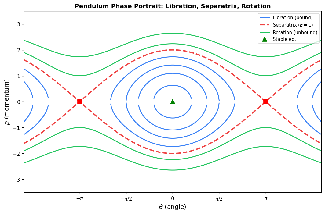
The example the professor gives to build intuition is the double pendulum constrained to a plane. Each pendulum arm sweeps through an angle \(q_1, q_2 \in [0, 2\pi)\), so the configuration space is a torus \(\mathcal{Q} = T^2 = S^1 \times S^1\). The topology of \(\mathcal{Q}\) is not trivially Euclidean, and this has physical consequences — it means you cannot use a single global coordinate chart to describe all configurations simultaneously.
The trajectory of the system is a parametric curve \(\mathsf{q}(s)\) in \(\mathcal{Q}\), where \(s\) is an evolution parameter (typically time). At each point \(\mathsf{q}\) along the trajectory, one can construct the tangent space \(T_\mathsf{q}\mathcal{Q}\): the vector space of all tangent vectors to curves through \(\mathsf{q}\). The generalized velocity \(\dot{q}^a = \mathrm{d}q^a/\mathrm{d}s\) is an element of \(T_\mathsf{q}\mathcal{Q}\). The union of all tangent spaces,
\[ \mathsf{T}\mathcal{Q} = \bigsqcup_{\mathsf{q} \in \mathcal{Q}} T_\mathsf{q}\mathcal{Q}, \]is the velocity phase space, or the tangent fibre bundle to \(\mathcal{Q}\). It is itself a \(2n\)-dimensional differentiable manifold. The Lagrangian formulation lives here: the Lagrangian \(L(\mathsf{q}, \dot{\mathsf{q}}, t)\) is a function on \(\mathsf{T}\mathcal{Q} \times \mathbb{R}\), and the physical trajectories are the extrema of the action integral \(\int L\,\mathrm{d}s\).
1.2 The Legendre Transform
The bridge between the Lagrangian and Hamiltonian formulations is the Legendre transform. Its role is to trade the velocity variables \(\dot{q}^a\) for the momentum variables \(p_a\), passing from the tangent bundle \(\mathsf{T}\mathcal{Q}\) to the cotangent bundle \(\mathsf{T}^*\mathcal{Q}\). Understanding this transform abstractly pays dividends throughout the course.
The maximum is attained where \(\partial f / \partial v^a = 0\), which gives the stationarity condition
\[ \frac{\partial l}{\partial v^a} = p_a. \]This equation identifies \(\mathsf{p}\) with the gradient of \(l\), and convexity ensures the map \(\mathsf{v} \mapsto \mathsf{p}\) is invertible. Substituting the maximising \(\mathsf{v}(\mathsf{p})\) back in gives \(h(\mathsf{p}) = f[\mathsf{p}, \mathsf{v}(\mathsf{p})]\). The transform is involutive: the Legendre transform of the Legendre transform returns the original function. The domain of \(h\) need not be all of \(V^*\) — for instance, the function \(l(v) = e^v\) has Legendre transform \(h(p) = p \log p - p\), defined only for \(p > 0\).
Applied to classical mechanics, the Legendre transform of the Lagrangian \(L(\mathsf{q}, \dot{\mathsf{q}}, t)\) with respect to the velocities \(\dot{q}^a\) gives the Hamiltonian:
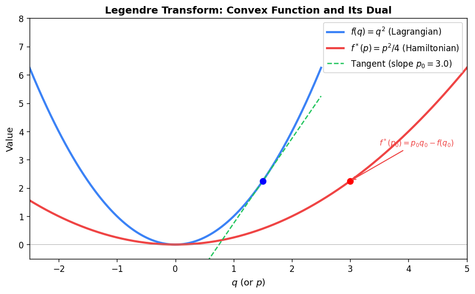
where the canonical momentum is \(p_a = \partial L / \partial \dot{q}^a\). The requirement that the Lagrangian be non-singular — that the Hessian \(D_{ab} = \partial^2 L / \partial \dot{q}^a \partial \dot{q}^b\) be positive definite — guarantees the Legendre transform is well-defined everywhere.
1.3 Hamilton’s Equations
From the Legendre transform one derives Hamilton’s equations of motion, the first-order reformulation of the Euler-Lagrange equations:
\[ \frac{\partial H}{\partial q^a} = -\dot{p}_a, \qquad \frac{\partial H}{\partial p_a} = \dot{q}^a. \]These are two sets of \(n\) first-order ODEs in \(2n\) variables, as opposed to the \(n\) second-order Euler-Lagrange equations. The equivalence is exact when the Legendre transform is non-degenerate. A beautiful consequence is that the time dependence of the Hamiltonian along a physical trajectory is entirely determined by its explicit time dependence:
\[ \dot{H} = \frac{\mathrm{d}H}{\mathrm{d}t} = \frac{\partial H}{\partial q^a}\dot{q}^a + \frac{\partial H}{\partial p_a}\dot{p}_a + \frac{\partial H}{\partial t} = \frac{\partial H}{\partial t}, \]since the first two terms cancel by Hamilton’s equations. If \(H\) has no explicit time dependence, it is conserved — this is the mechanical energy.
1.4 Phase Space
The Hamiltonian description lives not on the tangent bundle but on the cotangent bundle \(\mathsf{T}^*\mathcal{Q}\), also called phase space. The distinction is important: velocities \(\dot{q}^a\) are tangent vectors — elements of the tangent space at \(\mathsf{q}\) — while momenta \(p_a\) are one-forms, elements of the dual tangent space (the cotangent space). The canonical momentum \(p_a = \partial L / \partial \dot{q}^a\) is naturally a linear map from velocities to scalars, which is precisely the definition of a one-form.
The cotangent space at each point \(\mathsf{q} \in \mathcal{Q}\) is denoted \(T^*_\mathsf{q}\mathcal{Q}\), and the total space
\[ \mathsf{T}^*\mathcal{Q} = \bigsqcup_{\mathsf{q} \in \mathcal{Q}} T^*_\mathsf{q}\mathcal{Q} \]is the phase space: a \(2n\)-dimensional manifold carrying the points \((\mathsf{q}, \mathsf{p})\). Physical classical trajectories are curves in \(\mathsf{T}^*\mathcal{Q}\) whose tangent vector is determined by the Hamiltonian via Hamilton’s equations. Functions \(f(\mathsf{q}, \mathsf{p})\) on phase space are called dynamical variables.
For the pendulum example, the configuration space is the circle \(\mathcal{Q} = S^1\). At each angle \(\theta\) the cotangent space is \(\mathbb{R}\), so phase space is the cylinder \(\mathsf{T}^*\mathcal{Q} = S^1 \times \mathbb{R}\) — a familiar picture from introductory mechanics.
1.5 Poisson Brackets
To unify the dynamics of all dynamical variables under a single algebraic operation, one introduces the Poisson bracket. Working in the \(2n\) canonical variables \(\xi^\alpha = (q^1, \ldots, q^n, p_1, \ldots, p_n)\), the Poisson bracket of two dynamical variables \(f, g\) is
The Poisson bracket has four key properties. First, it is antisymmetric: \(\{f, g\} = -\{g, f\}\). Second, it satisfies the Jacobi identity: \(\{f,\{g,h\}\} + \{g,\{h,f\}\} + \{h,\{f,g\}\} = 0\). Third, it is bilinear: \(\{af+bg, h\} = a\{f,h\} + b\{g,h\}\). Fourth, it satisfies the Leibniz rule: \(\{fg, h\} = f\{g,h\} + g\{f,h\}\).
Together, antisymmetry and bilinearity make \(\mathcal{F}(\mathsf{T}^*\mathcal{Q})\) into a Lie algebra. Bilinearity and the Leibniz rule mean that taking the Poisson bracket with any fixed dynamical variable \(g\) acts as a derivation — a differential operator on phase space. In particular, the derivation associated with \(\xi^\alpha\) gives the Hamiltonian vector field:
\[ X^\alpha_f := \{\xi^\alpha, f\} = \tilde\Omega^{\alpha\beta}\partial_\beta f. \]Hamilton’s equations acquire a beautiful compact form: the time evolution of any canonical variable is \(\dot{\xi}^\alpha = \{\xi^\alpha, H\}\). More generally, for any dynamical variable \(f\) (possibly time-dependent),
\[ \dot{f} = \{f, H\} + \partial_t f. \]This is the equation of motion in Poisson bracket form, the classical precursor to Heisenberg’s equation.
1.6 The Symplectic Form
The antisymmetric matrix \(\tilde\Omega_{\alpha\beta}\) that appeared in the Poisson bracket is the component representation of a globally-defined geometric object called the symplectic form \(\boldsymbol\Omega\). In canonical coordinates,
\[ \boldsymbol\Omega = \frac{1}{2}\tilde\Omega_{\alpha\beta}\,\mathrm{d}\xi^\alpha \wedge \mathrm{d}\xi^\beta = \mathrm{d}p_a \wedge \mathrm{d}q^a. \]The symplectic form is a closed, non-degenerate two-form. Closure (\(\mathrm{d}\boldsymbol\Omega = 0\)) implies, by the Poincaré lemma, that locally \(\boldsymbol\Omega = \mathrm{d}\boldsymbol\theta\) for a one-form \(\boldsymbol\theta\) called the canonical form; in canonical coordinates \(\boldsymbol\theta = p_a \mathrm{d}q^a\). Non-degeneracy means that the symplectic matrix \(\tilde\Omega_{\alpha\beta}\) is invertible, allowing it to play a role analogous to the metric tensor in Riemannian geometry: it defines an isomorphism \(i_\mathsf{X}\boldsymbol\Omega : T(\mathsf{T}^*\mathcal{Q}) \to T^*(\mathsf{T}^*\mathcal{Q})\) taking each vector field \(\mathsf{X}\) to a one-form.
In canonical coordinates the symplectic matrix and its inverse are
\[ (\tilde\Omega_{\alpha\beta}) = \begin{pmatrix} 0_n & -\mathbb{1}_n \\ \mathbb{1}_n & 0_n \end{pmatrix}, \qquad (\tilde\Omega^{\alpha\beta}) = \begin{pmatrix} 0_n & \mathbb{1}_n \\ -\mathbb{1}_n & 0_n \end{pmatrix}. \]The symplectic matrix is antisymmetric (\(\tilde\Omega_{\alpha\beta} = -\tilde\Omega_{\beta\alpha}\)) and satisfies \(\tilde\Omega^2 = -\mathbb{1}\), making it a complex structure. Note that \(\tilde\Omega^{-1} = -\tilde\Omega = \tilde\Omega^\mathsf{T}\).
1.7 Hamilton’s Equations Without Coordinates
The coordinate-free version of Hamilton’s equations is compact and elegant. Given a Hamiltonian \(H\), it defines a unique vector field \(\mathsf{X}_H\) (the Hamiltonian vector field) via
\[ i_{\mathsf{X}_H}\boldsymbol\Omega = -\mathrm{d}H. \]The classical trajectories are the integral curves of \(\mathsf{X}_H\): curves \(\zeta(t)\) in phase space satisfying \(\dot\zeta^\alpha = X^\alpha_H\). In canonical coordinates, this single equation encodes both Hamilton equations simultaneously.
This formulation reveals a deep duality: each Hamiltonian \(H\) determines a unique dynamical vector field \(\mathsf{X}_H\), and conversely, if a vector field’s flow satisfies the evolution equation for Poisson brackets, then (locally) there exists a Hamiltonian generating that flow — unique up to an additive constant. This additive ambiguity is the familiar “origin of potential energy” freedom in mechanics.
1.8 Flows and the Lie Derivative
The flow of a vector field \(\mathsf{X}\) is the one-parameter family of maps \(\{\varphi_s^\mathsf{X}\}_{s \in \mathbb{R}}\) on phase space, where \(\varphi_s^\mathsf{X}(\boldsymbol\zeta)\) is the point reached from \(\boldsymbol\zeta\) by following the integral curves of \(\mathsf{X}\) for parameter distance \(s\). These maps form a group under composition: \(\varphi_{s_1}^\mathsf{X} \circ \varphi_{s_2}^\mathsf{X} = \varphi_{s_1+s_2}^\mathsf{X}\).
The infinitesimal action of the flow on any tensor field \(\mathbf{W}\) on phase space is given by the Lie derivative:
\[ \varphi^\mathsf{X}_{\delta s}\,\mathbf{W} = \mathbf{W} + \delta s\,(\mathcal{L}_\mathsf{X} + \partial_s)\mathbf{W}. \]For a finite displacement \(s\), the flow acts as an exponential of the Lie derivative:
\[ \varphi^\mathsf{X}_s = e^{s(\mathcal{L}_\mathsf{X} + \partial_s)}. \]On scalar dynamical variables \(g(\boldsymbol\zeta)\), the Lie derivative simplifies to the directional derivative along \(\mathsf{X}\):
\[ \mathcal{L}_\mathsf{X} g = X^\alpha_f \partial_\alpha g = \{g, f\}, \]so the Hamiltonian flow acting on any scalar \(g\) is
\[ \varphi^f_s g = e^{s(\{\ \cdot\ ,f\} + \partial_s)} g. \]This is the classical counterpart of the quantum time-evolution operator: it tells us how any observable quantity evolves when the system is “pushed” along the Hamiltonian flow.
1.9 Hamiltonian Flows as Canonical Transformations
The flow \(\varphi^f\) generated by any dynamical variable \(f\) is a Hamiltonian flow. Each dynamical variable \(f\) serves as the generating function of its associated Hamiltonian flow. The physical interpretation is especially clean for the canonical momenta: the projection of \(\mathsf{p}\) onto a direction \(v^a\) in configuration space generates translations in that direction, via the exponential map \(\varphi^f_s g = e^{s v^a \partial_{q^a}} g\).
\[ \dot{f} = \mathcal{L}_{\mathsf{X}_H} f + \partial_t f = \{f, H\} + \partial_t f. \]\[ \dot{\mathbf{W}} = \mathcal{L}_{\mathsf{X}_H}\mathbf{W} + \partial_t \mathbf{W}. \]1.10 Symplectic Manifolds
The cotangent bundle \(\mathsf{T}^*\mathcal{Q}\) is just one example of a symplectic manifold: a differentiable manifold \(\mathcal{M}\) of dimension \(2n\) equipped with a closed, non-degenerate two-form \(\boldsymbol\Omega\). The pair \((\mathcal{M}, \boldsymbol\Omega)\) is the symplectic manifold.
On any symplectic manifold, each smooth function \(H\) determines a Hamiltonian vector field \(\mathsf{X}_H\) via \(i_{\mathsf{X}_H}\boldsymbol\Omega = -\mathrm{d}H\), and the Poisson bracket is defined by
\[ \{f, g\} := \mathsf{X}_g f = -\boldsymbol\Omega(\mathsf{X}_f, \mathsf{X}_g) = \Omega^{\alpha\beta}\partial_\alpha f\,\partial_\beta g. \]This Poisson bracket is automatically antisymmetric (because \(\boldsymbol\Omega\) is a two-form), and the Jacobi identity follows from the closure condition \(\mathrm{d}\boldsymbol\Omega = 0\). Distinct choices of two-form on the same manifold \(\mathcal{M}\) yield different symplectic structures — mechanics on the same configuration space but with different “kinematic rules.”
1.11 Symplectic Transformations
A symplectic transformation (also called a canonical transformation) is a diffeomorphism \(\boldsymbol\zeta \to \boldsymbol\zeta'\) on phase space that preserves the symplectic form:
\[ \boldsymbol\Omega[\boldsymbol\zeta'(\boldsymbol\zeta)] - \boldsymbol\Omega(\boldsymbol\zeta) = 0. \]In components, the transformation \(\xi^\alpha \to \zeta^\alpha\) is symplectic if and only if
\[ \Omega_{\gamma\delta}(\boldsymbol\zeta')\,\partial_\alpha\zeta'^\gamma\,\partial_\beta\zeta'^\delta - \Omega_{\alpha\beta}(\boldsymbol\xi) = 0. \]There are four equivalent characterizations. A transformation is symplectic if and only if (1) the Lie derivative of \(\boldsymbol\Omega\) along its generating vector field \(\mathsf{X}\) vanishes, \(\mathfrak{L}_\mathsf{X}\boldsymbol\Omega = 0\); (2) its generating vector is Hamiltonian, meaning there exists \(f\) with \(i_\mathsf{X}\boldsymbol\Omega = -\mathrm{d}f\); (3) it preserves Poisson brackets, \(\{\zeta^\alpha, \zeta^\beta\}_\xi = \{\zeta^\alpha, \zeta^\beta\}_{\zeta'}\); or (4) it is generated by Hamiltonian evolution (Hamiltonian flows are always symplectic).
The group of symplectic transformations on \(\mathbb{R}^{2n}\) is the symplectic group \(\mathrm{Sp}(2n, \mathbb{R})\), the set of real \(2n \times 2n\) matrices \(S\) satisfying \(S\Omega S^\mathsf{T} = \Omega\).
1.12 Liouville’s Theorem
One of the deepest results in classical statistical mechanics is that Hamiltonian evolution preserves the phase-space volume element
\[ \boldsymbol{v} = \bigwedge_{a=1}^n \mathrm{d}p_a \wedge \mathrm{d}q^a = \frac{1}{n!}\boldsymbol\Omega^{\wedge n}. \]Liouville’s theorem states that this volume form is invariant under any Hamiltonian flow. The proof is elegant: since \(\boldsymbol\Omega\) is preserved by symplectic transformations (including Hamiltonian evolution), and \(\boldsymbol{v}\) is a simple function of \(\boldsymbol\Omega\) (its \(n\)-th exterior power), \(\boldsymbol{v}\) is also preserved.
More concretely, this means that however a region \(\mathcal{U}\) of phase space deforms under Hamiltonian evolution, its volume \(\int_\mathcal{U}\boldsymbol{v}\) remains constant:
\[ \int_{\varphi_s^f\mathcal{U}}\boldsymbol{v} = \int_\mathcal{U} \varphi_{-s}^f \boldsymbol{v} = \int_\mathcal{U}\boldsymbol{v}. \]This has a profound physical consequence: information is never lost in Hamiltonian dynamics. Phase-space volumes are incompressible, so the statistical ensemble describing our knowledge of the system cannot concentrate over time — quantum-mechanically, this is related to unitarity.
1.13 Statistical Mechanics on Phase Space
When one cannot track every particle in a system of \(N\) particles, one resorts to a statistical description. A density distribution \(\rho(\boldsymbol\xi, t)\) on phase space represents the probability density that the system’s state lies in an infinitesimal volume around \(\boldsymbol\xi\), normalized so that
\[ \int \rho(\boldsymbol\xi, t)\,\mathrm{d}^{2n}\xi = 1. \]By Liouville’s theorem, the probability in any phase-space region is conserved under Hamiltonian evolution. Applying Gauss’s theorem yields
\[ \dot\rho = 0 \implies \partial_t\rho = -\{\rho, H\}, \]the Liouville equation. This is the exact analogue, in classical statistical mechanics, of the quantum von Neumann equation \(\partial_t\hat\rho = -\frac{\mathrm{i}}{\hbar}[\hat H, \hat\rho]\). The expectation value of any dynamical variable \(f\) in the statistical state \(\rho\) is
\[ \langle f(q,p)\rangle_\rho = \iint \mathrm{d}q\,\mathrm{d}p\;\rho(q,p)\,f(q,p). \]This classical picture — states as probability distributions on phase space, observables as functions, expectation values as phase-space integrals — is precisely what quantum mechanics will modify in the next chapter.
Chapter 2: Quantizing Phase Space
2.1 Canonical Quantization and Its Discontents
Canonical quantization is the most familiar route from classical to quantum mechanics. Given a classical system described by canonical variables \((q^a, p_a)\) and a Hamiltonian \(H\), canonical quantization is a linear map — denoted by a hat — from (a subalgebra of) the classical dynamical variables to self-adjoint operators on a Hilbert space \(\mathcal{H}\):
\[ f(q,p) \;\longmapsto\; \hat{A}_f = f(\hat{q}, \hat{p}). \]\[ [\hat{o}, \hat{o}'] = \mathrm{i}\hbar\,\widehat{\{o, o'\}}, \]and (2) be irreducible: no proper subspace of \(\mathcal{H}\) is invariant under all the represented observables.
The factor \(\mathrm{i}\hbar\) deserves explanation. The Poisson bracket of two real (classical) functions is real, but the commutator of two self-adjoint operators is anti-self-adjoint. Multiplying by \(\mathrm{i}\hbar\) converts the commutator into the commutator divided by \(\mathrm{i}\hbar\), which is self-adjoint — so both sides of the quantization rule map real quantities to real quantities.
\[ \mathbb{1} \mapsto \hat{\mathbb{1}}, \qquad q \mapsto \hat{q} = q, \qquad p \mapsto \hat{p} = -\mathrm{i}\hbar\partial_q. \]These generate the Heisenberg algebra \(\{1, q, p\}\) with commutation relation \([\hat{q}, \hat{p}] = \mathrm{i}\hbar\).
However, canonical quantization runs into a fundamental obstruction: Groenewold’s theorem (1946) states that it is impossible to simultaneously satisfy both conditions (irreducibility and the Poisson bracket rule) for all smooth functions on phase space. There are simply too many classical observables. In practice one selects a complete set of classical observables — a set closed under Poisson brackets with respect to which every other observable that commutes with all of them is a multiple of the identity — and quantizes that set. The issue of factor ordering then appears immediately for products of non-commuting operators.
The density function \(\rho(q,p)\) describing a classical statistical state also has a quantum counterpart: the density operator \(\hat\rho\). In quantum mechanics \(\hat\rho\) is a positive semi-definite operator of unit trace acting on \(\mathcal{H}\). Because quantum mechanics has inherited the symplectic structure of classical mechanics — now encoded in commutation relations rather than Poisson brackets — it is natural to ask: can we represent \(\hat\rho\) as a phase-space distribution, just as we did for classical states?
2.2 Weyl Ordering
Before tackling the Wigner function, one needs a definite rule for ordering operator products. Weyl’s prescription (1927) is the most symmetric: place \(\hat{q}\) and \(\hat{p}\) in all possible relative positions in any monomial and take the average:
\[ q^m p^n \;\longmapsto\; \left.\frac{\partial^m}{\partial\lambda^m}\frac{\partial^n}{\partial\mu^n} \frac{(\lambda\hat{q}+\mu\hat{p})^{m+n}}{(m+n)!}\right|_{\lambda=\mu=0}. \]The key properties are: (1) if \(f(q,p) \in \mathbb{R}\) then \(\hat{A}_f\) is Hermitian; and (2) exponentials quantize cleanly: \(e^{\mathrm{i}(\lambda q + \mu p)} \mapsto e^{\mathrm{i}(\lambda\hat{q} + \mu\hat{p})}\). The Weyl rule does not respect products — \(\hat{A}_f\hat{A}_g \neq \hat{A}_{fg}\) in general — which is the source of the ordering ambiguity.
The density operator under Weyl ordering is the quantum image of the classical density function \(\rho(q,p)\). Knowing \(\hat\rho\) (a trace-class operator) is equivalent to knowing all its matrix elements — an infinite amount of data. The question Wigner posed in 1932 is: can we encode all of that information in a single phase-space function?
2.3 The Wigner Function
In 1932, Eugene Wigner introduced a function on phase space that encodes the full quantum state \(\hat\rho\) and recovers the classical phase-space distribution as the “classical limit.” His strategy was to symmetrize the position-space density matrix \(\rho(q'', q') := \langle q'' | \hat\rho | q'\rangle\) with respect to the two position arguments and Fourier transform one of them to momentum space.
Introducing centre-of-mass and relative coordinates \(q = (q''+q')/2\) and \(x = q'' - q'\), the Wigner function is defined as
The Wigner function is the Wigner-Weyl representation of the density operator: it is the function on phase space that corresponds to \(\hat\rho\) under the Weyl ordering scheme. Dually, for any Weyl-quantized observable \(\hat{A}_f\), the Wigner-Weyl representation of \(\hat{A}_f\) is
\[ A(q,p) := \int_{-\infty}^{\infty}\mathrm{d}x\; e^{-\frac{\mathrm{i}}{\hbar}px}\left\langle q+\tfrac{1}{2}x\,\Big|\,\hat{A}_f\,\Big|\,q-\tfrac{1}{2}x\right\rangle. \]A central result is that expectation values are computed exactly as in classical statistical mechanics:
\[ \langle \hat{A}_f \rangle_{\hat\rho} = \mathrm{Tr}(\hat\rho\,\hat{A}_f) = \iint \mathrm{d}q\,\mathrm{d}p\; W(q,p)\,A(q,p), \]where \(W(q,p)\) plays the role of the classical probability distribution and \(A(q,p)\) plays the role of the classical dynamical variable. This is the core promise of phase-space quantum mechanics: to reproduce quantum dynamics using the familiar formalism of classical statistical mechanics on phase space, at the cost of allowing \(W\) to take negative values.
2.4 Properties of the Wigner Function
\[ \iint \mathrm{d}q\,\mathrm{d}p\; W(q,p) = 1, \]corresponding to \(\mathrm{Tr}(\hat\rho) = 1\).
\[ \int_{-\infty}^{\infty}\mathrm{d}p\; W(q,p) = \langle q|\hat\rho|q\rangle = \rho(q), \]\[ \int_{\mathbb{R}}\mathrm{d}q\; W(q,p) = \langle p|\hat\rho|p\rangle = \rho(p). \]These are exactly the Born-rule probabilities for position and momentum measurements respectively.
\[ \mathrm{Tr}(\hat\rho_1\hat\rho_2) = 2\pi\hbar \iint \mathrm{d}q\,\mathrm{d}p\; W_1(q,p)\,W_2(q,p). \]\[ \iint \mathrm{d}q\,\mathrm{d}p\; [W(q,p)]^2 \leq \frac{1}{2\pi\hbar}, \]with equality for pure states.
\[ W(q,p) = \frac{1}{2\pi\hbar}\int_{-\infty}^{\infty}\mathrm{d}x\;e^{-\frac{\mathrm{i}}{\hbar}px}\psi\!\left(q+\tfrac{1}{2}x\right)\psi^*\!\left(q-\tfrac{1}{2}x\right). \]The bound \(|W(q,p)| \leq \frac{1}{\pi\hbar}\) follows from the Cauchy-Schwarz inequality applied to the \(L^2\) inner product of the two shifted wavefunctions.
Hudson’s theorem makes precise which states have non-negative Wigner functions: \(W(q,p) \geq 0\) for all \(q, p\) if and only if \(W\) is a Gaussian (and for pure states, the wavefunction is also Gaussian). The negativity of the Wigner function is a signature of genuine quantum features of the state — it signals the presence of quantum interference and non-classicality that cannot be captured by any positive phase-space distribution.
Folland-Sitaram theorem. \(W(q,p)\) has compact support if and only if \(W(q,p) = 0\) everywhere. In other words, no physical quantum state has a Wigner function that vanishes outside a bounded region.
Reality. \(\hat\rho^\dagger = \hat\rho\) implies \(W(q,p) \in \mathbb{R}\) for all \(q, p\).
Chapter 3: Quantum Dynamics in Phase Space
3.1 The Von Neumann Equation and the Moyal Bracket
\[ \frac{\partial\hat\rho}{\partial t} = -\frac{\mathrm{i}}{\hbar}[\hat H, \hat\rho]. \]This quantum equation of motion has a direct analogue for the Wigner function. Taking the time derivative of the definition of \(W\) and using the von Neumann equation, one can express \(\partial W/\partial t\) in terms of the Wigner function itself.
For a Hamiltonian of the mechanical energy type \(\hat H = \hat{p}^2/(2m) + U(\hat{q})\), the equation of motion for \(W\) splits into kinetic and potential terms:
\[ \frac{\partial W}{\partial t} = \mathcal{T} + \mathcal{U}, \]\[ \mathcal{T} = -\frac{p}{m}\frac{\partial}{\partial q}W(q,p), \qquad \mathcal{U} = \sum_{l=0}^{\infty} \frac{(\mathrm{i}\hbar/2)^{2l}}{(2l+1)!}\frac{\mathrm{d}^{2l+1}U(q)}{\mathrm{d}q^{2l+1}}\frac{\partial^{2l+1}}{\partial p^{2l+1}}W(q,p). \]The kinetic term \(\mathcal{T}\) is identical to its classical counterpart in the Liouville equation. The potential term \(\mathcal{U}\) contains the Liouville term \(l=0\) plus quantum corrections of order \(\hbar^2, \hbar^4, \ldots\). In the limit \(\hbar \to 0\), all but the \(l=0\) term vanish, and the quantum equation for \(W\) reduces to the classical Liouville equation \(\partial_t\rho = \{\rho, H\}\). This is the classical limit: the Wigner function satisfying the Moyal equation approaches the classical phase-space density in the limit of large action compared to \(\hbar\).
The Moyal bracket is the \(\hbar\)-deformation of the Poisson bracket, and the Wigner function formalism is a \(\star\)-product deformation of classical mechanics. This perspective — quantum mechanics as a deformation of classical mechanics on phase space — is the foundation of deformation quantization, a mathematically rigorous alternative to canonical quantization.
Chapter 4: Harmonic Oscillators, Coherent States, and Squeezed Light
4.1 The Harmonic Oscillator Ground State
The quantum harmonic oscillator with Hamiltonian
\[ \hat H = \frac{\hat{p}^2}{2m} + \frac{m\omega^2}{2}\hat{q}^2 = \hbar\omega\left(\hat{a}^\dagger\hat{a} + \frac{1}{2}\right) \]is the workhorse of quantum optics and quantum information with continuous variables. The annihilation and creation operators are
\[ \hat{a} = \sqrt{\frac{m\omega}{2\hbar}}\left(\hat{q} + \frac{\mathrm{i}}{m\omega}\hat{p}\right), \qquad \hat{a}^\dagger = \sqrt{\frac{m\omega}{2\hbar}}\left(\hat{q} - \frac{\mathrm{i}}{m\omega}\hat{p}\right), \]satisfying \([\hat{a}, \hat{a}^\dagger] = \mathbb{1}\). These operators are not quantum inventions — they are the Weyl quantization of the classical complex phase-space variables
\[ \alpha = \sqrt{\frac{m\omega}{2\hbar}}\left(q + \frac{\mathrm{i}}{m\omega}p\right), \qquad \alpha^* = \sqrt{\frac{m\omega}{2\hbar}}\left(q - \frac{\mathrm{i}}{m\omega}p\right). \]\[ \psi_0(q) = \frac{1}{(2\pi a_0^2)^{1/4}}e^{-q^2/(4a_0^2)}, \qquad a_0 = \sqrt{\frac{\hbar}{2m\omega}}. \]Substituting into the Wigner function formula gives
\[ W_{|0\rangle}(q,p) = \frac{1}{\pi\hbar}\exp\left(-\frac{q^2}{2a_0^2} - \frac{p^2}{2p_0^2}\right), \qquad p_0 = \frac{\hbar}{2a_0}. \]This is a circular Gaussian in phase space, centred at the origin. The product of the half-widths is
\[ p_0 a_0 = \frac{\hbar}{2} = \Delta q\,\Delta p, \]precisely the saturation of the Heisenberg uncertainty relation. The ground state has the smallest possible phase-space footprint consistent with quantum mechanics — it is a minimum uncertainty state.
This is the first example where the Wigner function is genuinely positive semidefinite, consistent with Hudson’s theorem: Gaussian Wigner functions arise from Gaussian wavefunctions.
4.2 Coherent States
Coherent states are the eigenstates of the annihilation operator. For any \(\alpha \in \mathbb{C}\),
Coherent states are generated from the vacuum by the displacement operator:
\[ \hat{D}(\alpha) := e^{\alpha\hat{a}^\dagger - \alpha^*\hat{a}} = e^{-|\alpha|^2/2}e^{\alpha\hat{a}^\dagger}e^{-\alpha^*\hat{a}}, \qquad \alpha \in \mathbb{C}, \]where the second equality follows from the Baker-Campbell-Hausdorff formula \(e^{\hat{A}+\hat{B}} = e^{-[\hat{A},\hat{B}]/2}e^{\hat{A}}e^{\hat{B}}\) when \([[\hat{A},\hat{B}],\hat{A}] = [[\hat{A},\hat{B}],\hat{B}] = 0\). One verifies that \(|\alpha\rangle = \hat{D}(\alpha)|0\rangle\) is indeed a coherent state by acting with \(\hat{a}\):
\[ \hat{a}|\alpha\rangle = e^{-|\alpha|^2/2}\sum_{n=0}^\infty \frac{\alpha^n}{\sqrt{n!}}\sqrt{n}|n-1\rangle = \alpha|\alpha\rangle. \]The Fock-state expansion \(|\alpha\rangle = e^{-|\alpha|^2/2}\sum_{n=0}^\infty \frac{\alpha^n}{\sqrt{n!}}|n\rangle\) shows that coherent states are Poisson superpositions of number states. The normalization \(\langle\alpha|\alpha\rangle = 1\) follows from \(\hat{D}(\alpha)\) being unitary.
A crucial — and initially counterintuitive — fact is that the creation operator \(\hat{a}^\dagger\) has no left eigenstate other than the zero vector. If \(\hat{a}^\dagger|\alpha'\rangle = \alpha'|\alpha'\rangle\), expanding in Fock states leads to \(c_0 = 0\) and by induction \(c_n = 0\) for all \(n\), so \(|\alpha'\rangle = 0\). This asymmetry between \(\hat{a}\) and \(\hat{a}^\dagger\) is a distinctly infinite-dimensional phenomenon — in finite-dimensional spaces over \(\mathbb{C}\), every operator has eigenvalues.
\[ \langle\alpha|\beta\rangle = e^{(-|\beta|^2-|\alpha|^2+2\beta\alpha^*)/2} \neq \delta(\alpha-\beta), \]\[ \frac{1}{\pi}\int \mathrm{d}^2\alpha\;|\alpha\rangle\langle\alpha| = \mathbb{1}. \]\[ \hat{D}^\dagger(\alpha)\hat{a}\hat{D}(\alpha) = \hat{a} + \alpha, \]which encodes the fact that \(\hat{D}(\alpha)\) shifts the quantum state by \(\alpha\) in phase space. This is the quantum counterpart of a phase-space translation.
4.3 The Wigner Function in the Coherent State Basis
The coherent state basis provides a computationally powerful representation of the Wigner function. After a calculation involving the change of variables to centre and relative coordinates and using the generating function of Hermite polynomials, one finds:
\[ W_{\hat\rho}(\alpha, \alpha^*) = \frac{1}{4\pi^2\hbar}\int \mathrm{d}\eta^*\mathrm{d}\eta\; e^{(\eta^*\alpha - \eta\alpha^*)}\langle\hat{D}(\eta)\rangle_{\hat\rho}, \]where the integration is over the complex plane (\(\mathrm{d}^2\eta = \mathrm{d}(\mathrm{Re}\,\eta)\,\mathrm{d}(\mathrm{Im}\,\eta)\)) and \(\langle\hat{D}(\eta)\rangle_{\hat\rho} = \mathrm{Tr}(\hat\rho\,\hat{D}(\eta))\) is the characteristic function of the state. This representation immediately yields the Wigner function of the vacuum:
\[ \langle\hat{D}(\eta)\rangle_{|0\rangle} = \langle 0|\hat{D}(\eta)|0\rangle = e^{-|\eta|^2/2}, \]and substituting gives the expected Gaussian
\[ W_{|0\rangle}(\alpha,\alpha^*) = \frac{1}{\pi\hbar}e^{-2|\alpha|^2}. \]A further simplification using the identity \(\hat T := \int\mathrm{d}^2\eta\,\hat{D}(\eta) = 2\pi e^{\mathrm{i}\pi\hat{a}^\dagger\hat{a}}\) gives the elegant formula:
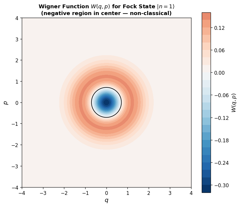
\[ W_{\hat\rho}(\alpha,\alpha^*) = \frac{1}{\pi\hbar}\left\langle \hat{D}(2\alpha)e^{\mathrm{i}\pi\hat{a}^\dagger\hat{a}}\hat{D}^\dagger(2\alpha)\right\rangle_{\hat\rho}, \]which leads directly to the Wigner function of the \(n\)-th Fock state:
For \(n=0\), \(L_0 = 1\) and we recover the Gaussian vacuum. For \(n \geq 1\), the Laguerre polynomial takes negative values, confirming that excited Fock states have negative Wigner functions — a clear signature of their non-classical character. The Wigner function of \(|n\rangle\) is highly oscillatory for \(|\alpha|^2 < n\) and decays rapidly for \(|\alpha|^2 > n\).
4.4 Single-Mode Squeezed States
Coherent states are displaced vacua — they saturate the Heisenberg uncertainty relation with equal spread in the two quadratures \(q\) and \(p\). Squeezed states are states that also saturate the uncertainty relation but distribute the uncertainty unequally between the two quadratures. By squeezing one quadrature to sub-vacuum noise levels, one can achieve enhanced precision in measurements of that quadrature.
The squeezing operator for a single mode is
\[ \hat{S}(\xi) = \exp\!\left[\frac{1}{2}\left(\xi^*\hat{a}^2 - \xi\hat{a}^{\dagger 2}\right)\right], \qquad \xi = r e^{\mathrm{i}\theta}, \]where \(r \geq 0\) is the squeezing parameter and \(\theta\) is the squeezing direction. The squeezing operator is unitary (\(\hat{S}^\dagger = \hat{S}^{-1} = \hat{S}(-\xi)\)) and preserves the phase-space area (it is symplectic). Its action on the ladder operators is a Bogoliubov transformation:
\[ \hat{S}^\dagger(\xi)\hat{a}\hat{S}(\xi) = \hat{a}\cosh r - \hat{a}^\dagger e^{\mathrm{i}\theta}\sinh r. \]The squeezed vacuum is \(\hat{S}(\xi)|0\rangle\). To express it in the Fock basis, one notes that the squeezing operator couples modes in pairs — each quantum of excitation in the first quadrature is created simultaneously with another — leading to:
\[ \hat{S}(\xi)|0\rangle = \frac{1}{\sqrt{\cosh r}}\sum_{n=0}^{\infty}\frac{\sqrt{(2n)!}}{2^n n!}(-e^{\mathrm{i}\theta}\tanh r)^n |2n\rangle. \]The squeezed vacuum is a superposition of even Fock states only — a consequence of the parity symmetry of the Hamiltonian generating the squeezing. The average energy of the squeezed vacuum is \(\langle 0|\hat{S}^\dagger\hat{a}^\dagger\hat{a}\hat{S}|0\rangle = \sinh^2 r\), which grows rapidly with \(r\): squeezing one quadrature costs energy.
The Wigner function of the squeezed vacuum is a squeezed Gaussian: the circular Gaussian of the vacuum is distorted into an ellipse aligned along the squeezing direction, with one axis compressed by a factor \(e^{-r}\) and the perpendicular axis expanded by \(e^r\), while the phase-space area remains equal to \(\hbar/2\).
4.5 Two-Mode Squeezed States
Now consider two harmonic oscillators with annihilation operators \(\hat{a}\) and \(\hat{b}\). The two-mode squeezing operator is
\[ \hat{S}(\xi) = \exp\!\left[\frac{1}{2}\left(\xi^*\hat{b}\hat{a} - \xi\hat{b}^\dagger\hat{a}^\dagger\right)\right], \qquad \xi = re^{\mathrm{i}\theta}, \]which couples the two modes. Its action on the ladder operators is
\[ \hat{S}^\dagger\hat{a}\hat{S} = \hat{a}\cosh r - \hat{b}^\dagger e^{\mathrm{i}\theta}\sinh r, \qquad \hat{S}^\dagger\hat{b}\hat{S} = \hat{b}\cosh r - \hat{a}^\dagger e^{\mathrm{i}\theta}\sinh r. \]The two-mode squeezed vacuum can be expressed in the Fock basis as
\[ \hat{S}(\xi)|0\rangle|0\rangle = \frac{1}{\cosh r}\sum_{n=0}^{\infty}(-e^{\mathrm{i}\phi}\tanh r)^n|n\rangle|n\rangle. \]This is a maximally entangled state in the continuous-variable setting. The excitation of the two modes is always correlated: a Fock state \(|n\rangle\) in one mode is always accompanied by \(|n\rangle\) in the other. The weight of the \(n\)-th term grows with the squeezing parameter \(r\), so more squeezing means stronger entanglement.
This result is the continuous-variable version of the Schmidt decomposition theorem: pure bipartite states always have mixed partial states, and the degree of mixedness measures the entanglement. It also hints at a deep connection between entanglement and thermality that becomes central to quantum field theory and the physics of black holes.
4.6 Weyl Quantization for \(n\) Degrees of Freedom
To handle systems of \(n\) coupled oscillators (or \(n\) field modes), one generalizes to the \(2n\)-dimensional symplectic vector space with canonical coordinates \(\boldsymbol\xi = (q^1, p_1, \ldots, q^n, p_n)\) (pairwise ordering). The symplectic form in pairwise canonical basis is
\[ (\tilde\Omega_{\alpha\beta}) = \bigoplus_{a=1}^n \begin{pmatrix} 0 & -1 \\ 1 & 0 \end{pmatrix}. \]One associates to each classical coordinate \(\xi^\alpha\) a self-adjoint operator \(\hat\Xi^\alpha\), with the canonical commutation relations
\[ [\hat\Xi(\boldsymbol\xi_1), \hat\Xi(\boldsymbol\xi_2)] = -\mathrm{i}\hbar\,\boldsymbol\Omega(\boldsymbol\xi_1, \boldsymbol\xi_2)\,\mathbb{1}, \]or in components, \([\hat\Xi^\beta, \hat\Xi^\delta] = \mathrm{i}\hbar\tilde\Omega^{\beta\delta}\mathbb{1}\). The generalized displacement operator is
\[ \hat{D}(\boldsymbol\xi) = e^{-\mathrm{i}\hat\Xi(\boldsymbol\xi)}, \]and it satisfies \(\hat{D}^\dagger(\boldsymbol\xi)\hat\Xi(\boldsymbol\xi')\hat{D}(\boldsymbol\xi) = \hat\Xi(\boldsymbol\xi') + \Omega(\boldsymbol\xi, \boldsymbol\xi')\mathbb{1}\).
The generalized Wigner function over the \(2n\)-dimensional phase space is
\[ W_{\hat\rho}(\boldsymbol\xi) := \frac{1}{(2\hbar\pi)^{2n}}\int\mathrm{d}^{2n}\boldsymbol\xi'\; e^{\frac{\mathrm{i}}{\hbar}\Omega(\boldsymbol\xi, \boldsymbol\xi')}\left\langle e^{-\frac{\mathrm{i}}{\hbar}\hat\Xi(\boldsymbol\xi')}\right\rangle_{\hat\rho}. \]For \(n=1\) this reduces to the single-mode Wigner function defined earlier. The \(n\)-mode generalization of the squeezing operator is
\[ \hat{S}_{\boldsymbol{F}} = e^{\frac{1}{2}F_{ab}\hat\Xi^a\hat\Xi^b}, \]where \(F_{ab}\) is a symmetric matrix. Under conjugation by \(\hat{S}_{\boldsymbol{F}}\), the quadrature operators undergo a symplectic transformation \(\hat\Xi(\boldsymbol\xi) \mapsto \hat\Xi(\boldsymbol{C}\boldsymbol\xi)\) where \(C^\alpha{}_\beta = (e^{\Omega F})^\alpha{}_\beta\).
Chapter 5: Gaussian Quantum Mechanics
5.1 Gaussian States and Covariance Matrices
A quantum state \(\hat\rho\) is called Gaussian if its Wigner function is a Gaussian distribution on phase space:
\[ W(\boldsymbol\xi) = \frac{1}{(\hbar\pi)^n\sqrt{\det\boldsymbol\sigma}}\exp\!\left(-(\boldsymbol\xi - \boldsymbol\xi_0)^\mu(\boldsymbol\xi - \boldsymbol\xi_0)^\nu(\boldsymbol\sigma^{-1})_{\mu\nu}\right). \]Two objects completely characterize a Gaussian state.
The covariance matrix is real, symmetric, and must satisfy
\[ \boldsymbol\sigma \geq \mathrm{i}\boldsymbol\Omega^{-1} \]as a matrix inequality (i.e., \(\boldsymbol\sigma - \mathrm{i}\boldsymbol\Omega^{-1}\) is positive semidefinite). This condition simultaneously enforces the positivity of \(\hat\rho\) and the uncertainty principle: it prevents the covariances from being arbitrarily small.
The power of the Gaussian formalism is that a Gaussian state of \(n\) modes — an operator on an infinite-dimensional Hilbert space — is completely specified by the \(n(2n+3)\) real numbers comprising \(\boldsymbol\xi_0\) and \(\boldsymbol\sigma\). One never needs to work with infinite-dimensional Hilbert spaces or operators explicitly.
Thermal state example. For a single harmonic oscillator in thermal equilibrium at temperature \(T\), the density operator is \(\hat\rho = Z^{-1}e^{-\beta\hat H}\) with \(\beta = 1/(k_\mathrm{B}T)\). The expectation values of \(\hat{q}\) and \(\hat{p}\) vanish (the thermal distribution is symmetric), so \(\boldsymbol\xi_0 = 0\). In terms of the dimensionless quadratures \(\hat{\tilde q} = \sqrt{m\omega/\hbar}\,\hat{q}\) and \(\hat{\tilde p} = (m\omega\hbar)^{-1/2}\hat{p}\), the covariance matrix is
\[ \boldsymbol\sigma = \begin{pmatrix}\nu & 0 \\ 0 & \nu\end{pmatrix} = \nu\mathbb{1}, \qquad \nu = \coth\!\left(\frac{\hbar\omega}{2k_\mathrm{B}T}\right) \geq 1. \]As \(T \to 0\), \(\nu \to 1\) and the covariance matrix becomes the identity — the ground state. As \(T \to \infty\), \(\nu \to \infty\) reflecting the classically unlimited spread of the thermal distribution.
Single-mode squeezed vacuum example. For the squeezed vacuum \(\hat{S}(re^{\mathrm{i}\theta})|0\rangle\), the first moments are zero and the covariance matrix is
\[ (\sigma^{\mu\nu}) = \begin{pmatrix}\cosh 2r - \cos\theta\sinh 2r & -\sin\theta\sinh 2r \\ -\sin\theta\sinh 2r & \cosh 2r + \cos\theta\sinh 2r\end{pmatrix}. \]For \(\theta = 0\), the squeezing is along the \(q\)-axis: the \(qq\)-variance becomes \(e^{-2r}\) (squeezed below vacuum) and the \(pp\)-variance becomes \(e^{2r}\) (stretched above vacuum).
5.2 Multipartite Covariance Matrices
One of the most elegant features of the covariance matrix description is how it handles composite systems. If two subsystems A and B are completely uncorrelated, their joint covariance matrix is simply the direct sum:
\[ \boldsymbol\sigma_\mathrm{AB} = \boldsymbol\sigma_\mathrm{A} \oplus \boldsymbol\sigma_\mathrm{B}. \]This is the covariance-matrix analogue of the tensor product of density matrices. In general, for a bipartite system:
\[ \boldsymbol\sigma_\mathrm{AB} = \begin{pmatrix}\boldsymbol\sigma_\mathrm{A} & \boldsymbol\gamma_\mathrm{AB} \\ \boldsymbol\gamma_\mathrm{AB} & \boldsymbol\sigma_\mathrm{B}\end{pmatrix}, \]where \(\boldsymbol\gamma_\mathrm{AB}\) is the matrix of cross-correlators between the observables of the two subsystems. Tracing out one subsystem — computing the partial state — is trivially implemented by extracting the corresponding diagonal block of the joint covariance matrix. No Hilbert-space traces are required.
This feature makes the covariance matrix formalism ideal for analysing multimode entanglement.
5.3 Time Evolution in the Symplectic Formulation
Gaussian unitary transformations are those that preserve the Gaussian character of states. Since unitary transformations preserve the canonical commutation relations, they preserve the symplectic form — they are symplectic transformations on phase space. Any such transformation can be generated by a quadratic Hamiltonian:
\[ \hat H = \frac{1}{2}\hat\Theta^\alpha\hat\Theta^\beta F_{\alpha\beta} + \alpha_\nu\hat\Theta^\nu, \]where \(\boldsymbol{F}\) is a Hermitian matrix (i.e., \(F_{\alpha\beta} = F^*_{\beta\alpha}\)) and \(\boldsymbol\alpha\) is a real vector.
The Heisenberg equations for the quadrature operators reduce, after a calculation using the commutation relations, to a linear equation:
\[ \frac{\mathrm{d}}{\mathrm{d}t}\hat{\boldsymbol\Theta} = \boldsymbol\Omega^{-1}\!\left(\bar{\boldsymbol{F}}\hat{\boldsymbol\Theta} + \boldsymbol\alpha\mathbb{1}\right), \]where \(\bar{\boldsymbol{F}} = (\boldsymbol{F} + \boldsymbol{F}^\mathsf{T})/2\) is the symmetrized Hamiltonian matrix. This is a linear, first-order ODE for the operator-valued vector \(\hat{\boldsymbol\Theta}\), and its solution is:
\[ \hat{\boldsymbol\Theta}(t) = \boldsymbol{S}(t)\hat{\boldsymbol\Theta}(0) + \boldsymbol{d}(t)\mathbb{1}, \]where the symplectic evolution matrix is
\[ \boldsymbol{S}(t) = \exp\!\left(\boldsymbol\Omega^{-1}\bar{\boldsymbol{F}}\,t\right), \qquad \boldsymbol{d}(t) = \frac{\exp(\boldsymbol\Omega^{-1}\bar{\boldsymbol{F}}\,t) - \mathbb{1}_{2n}}{\boldsymbol\Omega^{-1}\bar{\boldsymbol{F}}}\boldsymbol\Omega^{-1}\boldsymbol\alpha. \]Unitarity of the quantum evolution implies that \(\boldsymbol{S}\) is a symplectic matrix: \(\boldsymbol{S}\boldsymbol\Omega^{-1}\boldsymbol{S}^\mathsf{T} = \boldsymbol\Omega^{-1}\).
The deep insight here is that an infinite-dimensional unitary transformation on Hilbert space is faithfully represented by a finite-dimensional symplectic transformation on phase space. For Gaussian states — and only for Gaussian states — one never needs to leave the comfortable finite-dimensional world of vectors and matrices.
The equations of motion for the covariance matrix and first-moment vector follow directly:
The covariance matrix evolves by a symplectic congruence: \(\boldsymbol\sigma \mapsto \boldsymbol{S}\boldsymbol\sigma\boldsymbol{S}^\mathsf{T}\). This is the Gaussian analogue of the von Neumann equation \(\hat\rho \mapsto \hat{U}\hat\rho\hat{U}^\dagger\).
Revisiting squeezing via the symplectic formulation. For the single-mode squeezing operator \(\hat{S}(re^{\mathrm{i}\theta})\), the associated Hamiltonian is quadratic with \(W = 0\) and \(G = -\frac{\mathrm{i}r}{2}e^{\mathrm{i}\theta}\). After computing the matrices \(\boldsymbol{F}\), \(\bar{\boldsymbol{F}}\), \(\boldsymbol\Omega^{-1}\bar{\boldsymbol{F}}\), and exponentiating, the symplectic matrix implementing the squeezing is:
\[ \boldsymbol{S} = \begin{pmatrix}\cosh r - \cos\theta\sinh r & -\sin\theta\sinh r \\ -\sin\theta\sinh r & \cosh r + \cos\theta\sinh r\end{pmatrix}. \]Applied to the ground state covariance matrix \(\boldsymbol\sigma_0 = \mathbb{1}\), this gives \(\boldsymbol\sigma_\mathrm{sq} = \boldsymbol{S}\mathbb{1}\boldsymbol{S}^\mathsf{T}\), recovering the squeezed vacuum covariance matrix of equation (1.5.30). No quantum mechanics was used — just linear algebra on phase space.
Chapter 6: Entropy and Entanglement of Gaussian States
6.1 The Williamson Theorem: Symplectic Diagonalization
Every real symmetric positive-definite matrix (hence every valid covariance matrix) can be brought to a canonical diagonal form by a symplectic transformation. This is the content of Williamson’s theorem (1936).
The set \(\{\nu_1, \ldots, \nu_n\}\) is the symplectic spectrum of \(\boldsymbol\sigma\), and its elements are called symplectic eigenvalues. Crucially, the symplectic eigenvalues are not the ordinary eigenvalues of \(\boldsymbol\sigma\). Instead, they are the moduli of the eigenvalues of the matrix \(\boldsymbol{M} = \boldsymbol\sigma\boldsymbol\Omega^{-1}\). To see this, note that under a symplectic transformation \(\boldsymbol{S}\):
\[ \boldsymbol{M}' = \boldsymbol\sigma'\boldsymbol\Omega^{-1} = \boldsymbol{S}\boldsymbol\sigma\boldsymbol{S}^\mathsf{T}\boldsymbol\Omega^{-1} = \boldsymbol{S}\boldsymbol\sigma\boldsymbol\Omega^{-1}\boldsymbol{S}^{-1} = \boldsymbol{S}\boldsymbol{M}\boldsymbol{S}^{-1}, \]so \(\boldsymbol{M}\) undergoes a similarity transformation, preserving its eigenvalues. In the Williamson normal form, the matrix \(\boldsymbol{M}_\mathrm{D} = \boldsymbol\sigma_\mathrm{D}\boldsymbol\Omega^{-1}\) has the block-diagonal form \(\bigoplus_i \begin{pmatrix}0 & \nu_i \\ -\nu_i & 0\end{pmatrix}\), with eigenvalues \(\{\pm\mathrm{i}\nu_i\}\). The symplectic eigenvalues are therefore the moduli of the eigenvalues of \(\boldsymbol\sigma\boldsymbol\Omega^{-1}\).
The physical interpretation of the Williamson theorem is profound: any Gaussian state can be mapped, by a Gaussian unitary (a symplectic transformation on phase space), to a product of thermal states, one per mode. The symplectic eigenvalue \(\nu_i\) is the thermal parameter of the \(i\)-th effective mode. The uncertainty principle requires \(\nu_i \geq 1\) for all \(i\) (in dimensionless quadrature units).
6.2 Von Neumann Entropy of a Gaussian State
The von Neumann entropy \(S(\hat\rho) = -\mathrm{Tr}(\hat\rho\log\hat\rho)\) is the quantum analogue of the Boltzmann–Gibbs entropy. For a Gaussian state, computing it directly from the density operator requires handling an infinite-dimensional Hilbert space. The Williamson theorem bypasses this entirely.
The key insight is that the symplectic diagonalization of \(\boldsymbol\sigma\) corresponds to a Gaussian unitary transformation \(\hat{U}\) that brings \(\hat\rho\) to a tensor product of thermal states:
\[ \hat\rho' = \hat{U}\hat\rho\hat{U}^\dagger = \hat\rho'_1 \otimes \hat\rho'_2 \otimes \cdots \otimes \hat\rho'_n. \]Since the von Neumann entropy is unitarily invariant (\(S(\hat\rho) = S(\hat{U}\hat\rho\hat{U}^\dagger)\)) and additive over tensor products (\(S(\hat\rho' \otimes \hat\sigma') = S(\hat\rho') + S(\hat\sigma')\)), the total entropy is
\[ S(\hat\rho) = \sum_{i=1}^n S(\hat\rho'_i). \]Each \(\hat\rho'_i\) is a thermal state with mean occupation number \(\bar{n}'_i = (\nu_i - 1)/2\), and its von Neumann entropy is
\[ S(\hat\rho'_i) = (1+\bar{n}'_i)\log(1+\bar{n}'_i) - \bar{n}'_i\log\bar{n}'_i. \]Rewriting in terms of the symplectic eigenvalue \(\nu_i = 2\bar{n}'_i + 1\):
For a pure state, \(\boldsymbol\sigma = \boldsymbol{S}\mathbb{1}\boldsymbol{S}^\mathsf{T}\) for some symplectic \(\boldsymbol{S}\), and all symplectic eigenvalues equal 1, giving \(S = 0\). For a single thermal mode with \(\nu = \coth(\hbar\omega/2k_\mathrm{B}T)\), the formula gives the standard Bose-Einstein entropy.
The practical algorithm to compute the entropy of a Gaussian state is simply: (1) compute \(\boldsymbol\sigma\boldsymbol\Omega^{-1}\); (2) find its eigenvalues; (3) the symplectic eigenvalues are the moduli of the purely imaginary eigenvalues; (4) plug into the entropy formula. No infinite-dimensional computation is needed.
6.3 Entanglement Entropy of Coupled Harmonic Oscillators
To illustrate the full power of the symplectic formalism, consider two identical quantum harmonic oscillators with mass \(m\) and frequency \(\omega\), coupled through a spring of strength \(\lambda\). The Hamiltonian is
\[ \hat H = \frac{1}{2m}(\hat{p}_1^2 + \hat{p}_2^2) + \frac{m\omega^2}{2}(\hat{q}_1^2 + \hat{q}_2^2) + \lambda(\hat{q}_1 - \hat{q}_2)^2, \]which is quadratic in the canonical variables, so the ground state is Gaussian.
Step 1: Normal modes. The system decouples under the symplectic transformation
\[ \boldsymbol{S}^{-1} = \frac{1}{\sqrt{2}}\begin{pmatrix}1 & 0 & -1 & 0 \\ 0 & 1 & 0 & -1 \\ 1 & 0 & 1 & 0 \\ 0 & 1 & 0 & 1\end{pmatrix}, \]which takes the local oscillator modes \((\hat{q}_1, \hat{p}_1, \hat{q}_2, \hat{p}_2)\) to two independent normal modes with frequencies
\[ \omega'_1 = \omega, \qquad \omega'_2 = \omega\sqrt{1 + \frac{4\lambda}{m\omega^2}} =: \omega\alpha. \]Step 2: Ground state covariance matrix. The ground state of the decoupled system has the direct-sum covariance matrix
\[ \boldsymbol\sigma' = \hbar\begin{pmatrix}\frac{1}{m\omega} & 0 & 0 & 0 \\ 0 & m\omega & 0 & 0 \\ 0 & 0 & \frac{1}{m\omega\alpha} & 0 \\ 0 & 0 & 0 & m\omega\alpha\end{pmatrix}. \]Transforming back to local modes via \(\boldsymbol\sigma = \boldsymbol{S}^{-1}\boldsymbol\sigma'(\boldsymbol{S}^{-1})^\mathsf{T}\) gives the correlated ground state covariance matrix:
\[ \boldsymbol\sigma = \hbar\begin{pmatrix}\frac{\alpha+1}{2\alpha m\omega} & 0 & \frac{\alpha-1}{2\alpha m\omega} & 0 \\ 0 & \frac{1}{2}(\alpha+1)m\omega & 0 & -\frac{1}{2}(\alpha-1)m\omega \\ \frac{\alpha-1}{2\alpha m\omega} & 0 & \frac{\alpha+1}{2\alpha m\omega} & 0 \\ 0 & -\frac{1}{2}(\alpha-1)m\omega & 0 & \frac{1}{2}(\alpha+1)m\omega\end{pmatrix}. \]The off-diagonal blocks \(\boldsymbol\gamma_{12}\) reveal correlations between the two oscillators — they vanish when \(\lambda = 0\) (so \(\alpha = 1\)), as expected.
Step 3: Partial state and entanglement. Since the ground state is pure, the entanglement entropy is the von Neumann entropy of either partial state. The partial covariance matrix of oscillator 1 is the upper-left \(2\times 2\) block:
\[ \boldsymbol\sigma_1 = \boldsymbol\sigma_2 = \hbar\begin{pmatrix}\frac{\alpha+1}{2\alpha m\omega} & 0 \\ 0 & \frac{1}{2}(\alpha+1)m\omega\end{pmatrix}. \]Step 4: Symplectic eigenvalue. Taking \(\hbar = 1\) for simplicity, the unique symplectic eigenvalue of \(\boldsymbol\sigma_1\) (the modulus of the imaginary eigenvalues of \(\boldsymbol\sigma_1\boldsymbol\Omega^{-1}\)) is
\[ \nu = \frac{1+\alpha}{2\sqrt{\alpha}}. \]As \(\lambda \to 0\), \(\alpha \to 1\) and \(\nu \to 1\) — the vacuum, with zero entropy. As \(\lambda \to \infty\), \(\alpha \to \infty\) and \(\nu \to \infty\) — the partial state becomes infinitely mixed, with diverging entropy.
Step 5: Entanglement entropy. The entanglement entropy of the ground state is
\[ S_E = \frac{\nu+1}{2}\log\frac{\nu+1}{2} - \frac{\nu-1}{2}\log\frac{\nu-1}{2}, \]which is a monotonically increasing function of the coupling strength \(\lambda\). This result — the entanglement in the ground state of a coupled harmonic system computed from a \(2\times 2\) matrix eigenvalue problem — illustrates the remarkable economy of the Gaussian formalism. The infinite-dimensional quantum problem has been completely solved by a finite-dimensional classical computation.
Chapter 7: Quantum Channels and Quantum Operations
7.1 From Unitary Evolution to Open Dynamics
The quantum mechanics developed so far — Schrödinger’s equation, unitary time evolution, the Wigner function — describes closed systems: systems that are perfectly isolated from their environment. This is an idealization. Every real quantum system couples to its surroundings to some degree. Photons scatter off stray fields; atoms spontaneously emit into the electromagnetic vacuum; superconducting qubits are coupled to microscopic two-level defects in their substrates. The question is not whether a system couples to its environment but how to describe the resulting dynamics in terms of the system alone.
The appropriate mathematical language is the theory of quantum channels, also called quantum operations or completely positive maps. The key insight — due independently to Kraus (1983), and earlier in different language to Sudarshan and Stinespring — is that tracing out an environment from a joint unitary evolution always produces a map on density operators of a very specific form. Characterising this form without reference to any particular environment is the main result of the theory.
7.2 The Kraus Representation
The starting point is the most general evolution available: a joint unitary on system \(\mathcal{H}_S\) and environment \(\mathcal{H}_E\), followed by discarding the environment. If the environment begins in a fixed pure state \(|e_0\rangle\), the evolution of the system state is
\[ \hat\rho_S \;\longmapsto\; \mathcal{E}(\hat\rho_S) = \mathrm{Tr}_E\!\left[\hat{U}(\hat\rho_S \otimes |e_0\rangle\langle e_0|)\hat{U}^\dagger\right]. \]Inserting a resolution of the identity on \(\mathcal{H}_E\) in an orthonormal basis \(\{|e_k\rangle\}\),
\[ \mathcal{E}(\hat\rho_S) = \sum_k \langle e_k|\hat{U}|e_0\rangle\,\hat\rho_S\, \langle e_0|\hat{U}^\dagger|e_k\rangle. \]Defining the Kraus operators \(\hat{K}_k := \langle e_k|\hat{U}|e_0\rangle\) — operators on \(\mathcal{H}_S\) obtained by sandwiching the joint unitary between environment basis states — the map takes the form:
The completeness relation \(\sum_k \hat{K}_k^\dagger\hat{K}_k = \mathbb{1}\) is precisely the condition that \(\mathcal{E}\) is trace-preserving: \(\mathrm{Tr}[\mathcal{E}(\hat\rho)] = \mathrm{Tr}[\hat\rho] = 1\). The Kraus representation is not unique — any two representations \(\{\hat{K}_k\}\) and \(\{\hat{L}_j\}\) of the same channel are related by a unitary mixing \(\hat{L}_j = \sum_k u_{jk}\hat{K}_k\). This freedom reflects the fact that many different environments can induce the same channel on the system: the physics of the system is insensitive to which environment description one uses.
7.3 Complete Positivity
A channel \(\mathcal{E}\) must map density operators to density operators. In particular, \(\mathcal{E}\) must be positive: it must map positive semidefinite operators to positive semidefinite operators. But this is not sufficient. Consider a system \(S\) entangled with an ancilla \(A\) that is left untouched. If \(\mathcal{E}\) acts only on \(S\), the joint state evolves as \((\mathcal{E} \otimes \mathrm{id}_A)(\hat\rho_{SA})\). For this to remain a valid density operator for every entangled joint state \(\hat\rho_{SA}\), one needs the map \(\mathcal{E} \otimes \mathrm{id}_n\) to be positive for every ancilla dimension \(n\). This is a strictly stronger requirement.
The Kraus form is automatically completely positive — one can check directly that \((\mathcal{E} \otimes \mathrm{id}_A)(\hat\tau) = \sum_k (\hat{K}_k \otimes \mathbb{1}_A)\hat\tau(\hat{K}_k^\dagger \otimes \mathbb{1}_A)\) is positive for any positive \(\hat\tau\) on \(\mathcal{H}_S \otimes \mathcal{H}_A\). Conversely, the Kraus theorem says these are the only CPTP maps: CP + TP \(\Leftrightarrow\) Kraus form. The celebrated Stinespring dilation theorem adds that every CPTP map arises from an isometry \(\hat{V}: \mathcal{H}_S \to \mathcal{H}_S \otimes \mathcal{H}_E\) via \(\mathcal{E}(\hat\rho) = \mathrm{Tr}_E[\hat{V}\hat\rho\hat{V}^\dagger]\), giving the microscopic interpretation of every channel as an interaction with an environment.
A subtlety worth noting: the transpose map — sending \(\hat\rho \mapsto \hat\rho^\mathsf{T}\) — is positive (it preserves positive semidefinite operators) but not completely positive. The failure of complete positivity of the partial transpose is exploited in entanglement detection: the Peres-Horodecki positive partial transpose (PPT) criterion states that if a bipartite state \(\hat\rho_{AB}\) is separable, then \((\mathcal{T}_A \otimes \mathrm{id}_B)\hat\rho_{AB} \geq 0\). Any state with a negative partial transpose is therefore entangled. For Gaussian states, the PPT criterion is both necessary and sufficient for separability (the Simon criterion, 2000).
7.4 Important Examples of Quantum Channels
To build intuition, consider several standard channels acting on a single qubit.
The depolarizing channel replaces the qubit state with the maximally mixed state with probability \(p\) and leaves it unchanged with probability \(1-p\):
\[ \mathcal{E}_{\mathrm{dep}}(\hat\rho) = (1-p)\hat\rho + \frac{p}{3}(\hat{X}\hat\rho\hat{X} + \hat{Y}\hat\rho\hat{Y} + \hat{Z}\hat\rho\hat{Z}) = \left(1-\frac{4p}{3}\right)\hat\rho + \frac{4p}{3}\cdot\frac{\mathbb{1}}{2}, \]where \(\hat{X}, \hat{Y}, \hat{Z}\) are the Pauli matrices. The Kraus operators are \(\{\sqrt{1-p}\,\mathbb{1},\,\sqrt{p/3}\,\hat{X},\,\sqrt{p/3}\,\hat{Y},\,\sqrt{p/3}\,\hat{Z}\}\). Geometrically on the Bloch sphere, the depolarizing channel uniformly shrinks the Bloch vector by the factor \(1-4p/3\).
The amplitude damping channel models the spontaneous emission of a two-level atom: the excited state \(|1\rangle\) decays to the ground state \(|0\rangle\) by emitting a photon into the vacuum. With decay probability \(\gamma\):
\[ \hat{K}_0 = \begin{pmatrix}1 & 0 \\ 0 & \sqrt{1-\gamma}\end{pmatrix}, \qquad \hat{K}_1 = \begin{pmatrix}0 & \sqrt{\gamma} \\ 0 & 0\end{pmatrix}. \]The channel sends \(|1\rangle\langle 1| \to (1-\gamma)|1\rangle\langle 1| + \gamma|0\rangle\langle 0|\) (partial decay) and \(|0\rangle\langle 0| \to |0\rangle\langle 0|\) (ground state is stable). It has a unique fixed point — the ground state — unlike the depolarizing channel which fixes the maximally mixed state.
The phase damping (dephasing) channel destroys quantum coherences without energy exchange:
\[ \mathcal{E}_{\mathrm{deph}}(\hat\rho) = (1-p)\hat\rho + p\hat{Z}\hat\rho\hat{Z} = \begin{pmatrix}\rho_{00} & (1-2p)\rho_{01} \\ (1-2p)\rho_{10} & \rho_{11}\end{pmatrix}. \]The diagonal (population) elements are preserved while the off-diagonal (coherence) elements are suppressed by \(|1-2p|\). Complete dephasing (\(p = 1/2\)) destroys all coherences and turns any state into a classical mixture of energy eigenstates. This is precisely the quantum-to-classical transition that decoherence theory studies.
7.5 Gaussian Channels
The Gaussian formalism extends naturally to channels. A Gaussian channel is one that maps Gaussian states to Gaussian states. Just as Gaussian unitaries are represented by symplectic matrices, Gaussian channels are characterised by two matrices \((\boldsymbol{T}, \boldsymbol{N})\): a real matrix \(\boldsymbol{T}\) that transforms the covariance matrix as
\[ \boldsymbol\sigma \;\longmapsto\; \boldsymbol{T}\boldsymbol\sigma\boldsymbol{T}^\mathsf{T} + \boldsymbol{N}, \]and a positive semidefinite noise matrix \(\boldsymbol{N}\) added to the covariance matrix. The complete positivity constraint requires \(\boldsymbol{N} + \mathrm{i}(\boldsymbol\Omega^{-1} - \boldsymbol{T}\boldsymbol\Omega^{-1}\boldsymbol{T}^\mathsf{T}) \geq 0\). The first moments transform as \(\boldsymbol\xi_0 \mapsto \boldsymbol{T}\boldsymbol\xi_0 + \boldsymbol{d}\) for a displacement vector \(\boldsymbol{d}\).
The Gaussian framework makes the quantum capacity of Gaussian channels tractable — a problem that is in general extremely hard. The capacity of the Gaussian thermal noise channel was established in 2014 (Giovannetti et al.) and involves an optimization over Gaussian input states, which in the covariance matrix formalism reduces to a finite-dimensional semidefinite program.
Chapter 8: The Measurement Problem
8.1 What the Problem Is
Quantum mechanics is governed by two distinct dynamical rules. Between measurements, a closed quantum system evolves deterministically and unitarily according to the Schrödinger equation: \(\hat\rho(t) = \hat{U}(t)\hat\rho(0)\hat{U}^\dagger(t)\). During a measurement, the state appears to undergo an irreversible, probabilistic collapse: if a projective measurement of observable \(\hat{A} = \sum_a a\,\hat{P}_a\) is performed on a state \(\hat\rho\), the outcome \(a\) occurs with probability \(p_a = \mathrm{Tr}(\hat{P}_a\hat\rho)\), and the post-measurement state is \(\hat{P}_a\hat\rho\hat{P}_a / p_a\).
The measurement problem is the tension between these two rules. Measurement devices are themselves physical systems, and should therefore obey the Schrödinger equation. So why does measurement produce a definite outcome rather than leaving the pointer of the apparatus in a superposition? Bohr’s original answer — the Copenhagen interpretation — drew a sharp distinction between the quantum system and the classical measuring apparatus (“Heisenberg cut”), but offered no physical criterion for where to draw the line. John von Neumann formalised this in his Mathematical Foundations of Quantum Mechanics (1932) by showing that the cut can be placed anywhere in the measurement chain without changing the predicted probabilities — but the collapse must be placed somewhere to account for the definiteness of outcomes.
8.2 The Von Neumann Chain and the Heisenberg Cut
Von Neumann’s analysis proceeds as follows. Let the system \(S\) begin in a superposition \(|\psi_S\rangle = \sum_a c_a|a\rangle\) and the apparatus pointer \(A\) begin in a ready state \(|A_0\rangle\). An ideal measurement interaction (a pre-measurement) creates correlations:
\[ \left(\sum_a c_a|a\rangle\right) \otimes |A_0\rangle \;\xrightarrow{\hat{U}_\text{int}}\; \sum_a c_a|a\rangle \otimes |A_a\rangle, \]where \(|A_a\rangle\) are orthogonal pointer states. The joint state is now entangled. The reduced state of \(S\) is \(\hat\rho_S = \sum_a |c_a|^2|a\rangle\langle a|\) — identical to the classical mixture that would describe ignorance of which outcome occurred. But the global state is a coherent superposition, not a mixture: the joint state is pure, not a classical statistical ensemble.
This is the crux of the problem. Local statistics on either \(S\) or \(A\) are identical whether the global state is the entangled superposition or the corresponding classical mixture, but the two are physically distinct: the superposition still admits interference between branches, in principle. The measurement problem asks what physical process — and governed by which law — selects one branch.
8.3 Decoherence and Environment-Induced Superselection
The modern understanding of why macroscopic superpositions are not observed in practice is decoherence. The central insight, developed by Zurek and Joos among others from the 1980s, is that measurement devices are not isolated: they couple continuously to a vast environment (air molecules, photons, cosmic rays). This coupling selects a preferred basis — the pointer basis — in which the apparatus states are stable to environmental monitoring.
Once the environment \(E\) is coupled to the apparatus \(A\), the joint evolution is
\[ \sum_a c_a|a\rangle|A_a\rangle \;\xrightarrow{\hat{U}_{AE}}\; \sum_a c_a|a\rangle|A_a\rangle|E_a\rangle, \]where the environment states \(|E_a\rangle\) distinguish the pointer states. Tracing out the environment:
\[ \hat\rho_{SA} = \mathrm{Tr}_E\!\left[\sum_{a,b} c_a c_b^*|a\rangle\langle b| \otimes |A_a\rangle\langle A_b| \otimes |E_a\rangle\langle E_b|\right] = \sum_{a,b} c_a c_b^* \langle E_b|E_a\rangle |a\rangle\langle b| \otimes |A_a\rangle\langle A_b|. \]If the environment states rapidly become orthogonal, \(\langle E_b|E_a\rangle \to \delta_{ab}\), the off-diagonal terms in \(\hat\rho_{SA}\) vanish on the decoherence timescale \(\tau_D\). The joint state becomes indistinguishable from the classical mixture \(\sum_a |c_a|^2|a\rangle\langle a|\otimes|A_a\rangle\langle A_a|\).
The decoherence timescale \(\tau_D\) is extraordinarily short for macroscopic objects. For a dust grain of mass \(10^{-5}\) g coupled to air at room temperature, Zurek estimates \(\tau_D \sim 10^{-23}\) s — far shorter than any observable timescale. This explains why Schrödinger-cat superpositions are never observed in practice: they decohere instantaneously on any humanly relevant timescale.
8.4 What Decoherence Does and Does Not Solve
Decoherence explains why the off-diagonal elements of the density matrix — the interference terms — vanish so rapidly that they are unobservable. It also selects the preferred pointer basis: the set of states that are stable under monitoring by the environment. For the harmonic oscillator coupled to a thermal bath, the pointer states are coherent states — they decohere least rapidly because they are the “most classical” in the sense of minimising quantum back-action from the environment. This is the phenomenon of einselection (environment-induced superselection).
What decoherence does not solve is the preferred-outcome problem: after decoherence, the reduced density matrix \(\hat\rho_S\) is diagonal in the pointer basis, which is formally indistinguishable from a classical probability distribution — but it remains a description of an ensemble, not a single definite outcome. Explaining why any particular outcome occurs, and why we perceive only one branch of the superposition, requires additional interpretational input beyond the Schrödinger equation. This is where the various interpretations of quantum mechanics — Many-Worlds (Everett), relational QM (Rovelli), spontaneous collapse models (GRW, CSL), and QBism — part ways. The measurement problem remains, in this refined sense, an open question in the foundations of quantum mechanics.
Chapter 9: Open Quantum Systems and the Lindblad Equation
9.1 System-Environment Coupling
Chapter 7 described quantum channels — the most general maps on density operators consistent with complete positivity. But in many physical situations one needs a dynamical, time-local description: a differential equation governing the evolution of the reduced density matrix \(\hat\rho_S(t)\), analogous to the Schrödinger equation for closed systems. This is the purview of the theory of open quantum systems.
The starting point is the total Hamiltonian
\[ \hat{H}_\mathrm{tot} = \hat{H}_S \otimes \mathbb{1}_E + \mathbb{1}_S \otimes \hat{H}_E + \hat{H}_\mathrm{int}, \]where \(\hat{H}_S\) and \(\hat{H}_E\) are the free Hamiltonians of system and environment, and \(\hat{H}_\mathrm{int}\) is the coupling. The total state evolves unitarily, and the reduced state \(\hat\rho_S(t) = \mathrm{Tr}_E[\hat\rho_\mathrm{tot}(t)]\) evolves according to an exact but typically intractable integro-differential equation. Deriving a closed, tractable equation for \(\hat\rho_S(t)\) requires approximations.
9.2 The Born-Markov Approximation
Two standard approximations lead to a tractable equation. The Born approximation assumes the coupling is weak enough that the environment is negligibly disturbed by the interaction — the environment stays in its initial (typically thermal) state \(\hat\rho_E\) throughout. Formally: \(\hat\rho_\mathrm{tot}(t) \approx \hat\rho_S(t) \otimes \hat\rho_E\). The Markov approximation assumes the environment correlation functions decay rapidly on the timescale of system evolution: the environment has no memory, and the future evolution of \(\hat\rho_S\) depends only on its present state, not its history. Formally, if \(\tau_E\) is the environment correlation time and \(\tau_R\) is the relaxation timescale of the system, the Markov approximation requires \(\tau_E \ll \tau_R\).
Under these two approximations, the reduced dynamics takes the form of a first-order differential equation. The most general such equation that is both time-local and generates a completely positive and trace-preserving flow was independently derived by Gorini, Kossakowski, and Sudarshan (1976) and by Lindblad (1976):
The first term generates unitary Hamiltonian evolution. The second is the dissipator \(\mathcal{D}[\hat{L}_k]\hat\rho\), often written compactly as \(\mathcal{D}[\hat{L}_k]\hat\rho = \hat{L}_k\hat\rho\hat{L}_k^\dagger - \frac{1}{2}\{\hat{L}_k^\dagger\hat{L}_k,\hat\rho\}\). The specific anti-commutator structure \(-\frac{1}{2}\hat{L}_k^\dagger\hat{L}_k\hat\rho - \frac{1}{2}\hat\rho\hat{L}_k^\dagger\hat{L}_k\) is precisely what is needed to ensure trace preservation: \(\frac{\mathrm{d}}{\mathrm{d}t}\mathrm{Tr}[\hat\rho] = \mathrm{Tr}[\mathcal{D}[\hat{L}_k]\hat\rho] = 0\). The complete positivity is guaranteed by the positivity of the coefficients \(\gamma_k\).
A remarkable result due to Lindblad is that this form is uniquely determined by the requirements of complete positivity and trace preservation, along with the assumption that the generators are bounded operators. The GKSL equation is thus the quantum analogue of the Fokker-Planck equation in classical stochastic dynamics.
9.3 Physical Examples
Spontaneous emission. A two-level atom with excited state \(|e\rangle\) and ground state \(|g\rangle\) couples to the electromagnetic vacuum and emits photons at rate \(\Gamma\). The single jump operator is \(\hat{L} = |g\rangle\langle e|\) (de-excitation), and the master equation is
\[ \dot{\hat\rho} = -\frac{\mathrm{i}\omega_0}{2}[\hat\sigma_z, \hat\rho] + \Gamma\!\left(\hat\sigma_-\hat\rho\hat\sigma_+ - \frac{1}{2}\hat\sigma_+\hat\sigma_-\hat\rho - \frac{1}{2}\hat\rho\hat\sigma_+\hat\sigma_-\right), \]where \(\hat\sigma_\pm = (\hat{X} \pm \mathrm{i}\hat{Y})/2\) and \(\omega_0\) is the transition frequency. Solving for the matrix elements: the excited-state population decays as \(\rho_{ee}(t) = \rho_{ee}(0)e^{-\Gamma t}\), and the coherences decay as \(\rho_{eg}(t) = \rho_{eg}(0)e^{-(\mathrm{i}\omega_0 + \Gamma/2)t}\). The factor of \(\Gamma/2\) in the coherence decay — rather than \(\Gamma\) — reflects the fact that coherence is lost at half the rate of population, because the coherence is the geometric mean of the populations.
Pure dephasing. If the environment monitors the energy of the system without exchanging energy, the appropriate Lindblad operator is \(\hat{L} = \hat\sigma_z\) with rate \(\gamma_\phi\):
\[ \dot{\hat\rho} = \gamma_\phi\!\left(\hat\sigma_z\hat\rho\hat\sigma_z - \hat\rho\right) = \begin{cases}\dot\rho_{ee} = \dot\rho_{gg} = 0, \\ \dot\rho_{eg} = -2\gamma_\phi\rho_{eg}.\end{cases} \]Populations are conserved while coherences decay. The combined effect of spontaneous emission and dephasing gives the longitudinal relaxation time \(T_1 = 1/\Gamma\) and transverse relaxation time \(1/T_2 = \Gamma/2 + \gamma_\phi\) — the standard parameters of nuclear magnetic resonance and quantum computing.
9.4 The Lindblad Equation for Gaussian Systems
For Gaussian systems with quadratic Hamiltonians and linear Lindblad operators \(\hat{L}_k = \boldsymbol{\ell}_k^\mathsf{T}\hat{\boldsymbol\Theta}\), the Lindblad equation preserves Gaussian states and reduces to a closed set of first-order ODEs for the covariance matrix and first moments. The covariance matrix evolves as
\[ \dot{\boldsymbol\sigma} = \boldsymbol{A}\boldsymbol\sigma + \boldsymbol\sigma\boldsymbol{A}^\mathsf{T} + \boldsymbol{D}, \]where \(\boldsymbol{A} = \boldsymbol\Omega^{-1}\bar{\boldsymbol{F}} - \frac{1}{2}\boldsymbol\Gamma\) is the drift matrix (\(\boldsymbol\Gamma\) encodes the damping from the Lindblad operators) and \(\boldsymbol{D}\) is a positive semidefinite diffusion matrix encoding the noise injected by the environment. This is the quantum Fokker-Planck equation in covariance matrix form. In the long-time limit, the covariance matrix approaches the unique steady state determined by \(\boldsymbol{A}\boldsymbol\sigma_\infty + \boldsymbol\sigma_\infty\boldsymbol{A}^\mathsf{T} + \boldsymbol{D} = 0\) — a Lyapunov equation that can be solved numerically or, in special cases, analytically.
Non-Markovian effects become relevant when the environment correlation time \(\tau_E\) is comparable to the system timescale \(\tau_R\). In this regime, the memory of the environment must be retained, and the dynamics is governed by integro-differential equations (the Nakajima-Zwanzig equation). Non-Markovian dynamics can in principle be beneficial for quantum information processing: the back-flow of information from environment to system can be exploited to recover coherence. Quantifying non-Markovianity and its operational consequences is an active area of research.
Chapter 10: Relativistic Quantum Information and the Unruh-DeWitt Detector
10.1 Why Relativity and Quantum Theory Must Coexist
The frameworks developed in the preceding chapters — quantum channels, the measurement problem, open quantum systems — treat time as absolute: all observers agree on which instant is “now.” In relativity, simultaneity is observer-dependent. When quantum systems are coupled to relativistic fields, or when the curvature of spacetime is relevant, the separation between “system” and “environment” becomes observer-dependent too. This is not merely an exotic concern: the quantum vacuum itself, as seen from an accelerating observer, is indistinguishable from a thermal bath. Understanding quantum information in relativistic settings requires going beyond the non-relativistic theory.
The key tool for this enterprise is the particle detector model. Rather than asking what states of a quantum field mean in the abstract, one asks a concrete operational question: what does a localized, finite-size detector register when it couples to a quantum field? This is a physically well-posed question whose answer is observer-dependent in a precise, calculable way.
10.2 The Unruh-DeWitt Detector Model
The simplest particle detector model was proposed by Unruh and further developed by DeWitt. It consists of a two-level quantum system (a qubit, thought of as a hydrogen atom whose internal degrees of freedom are modelled as just a ground state \(|g\rangle\) and an excited state \(|e\rangle\)) coupled to a real scalar quantum field \(\hat\phi(\mathsf{x})\). The coupling is pointlike and linear in the field:
The monopole operator \(\hat\mu = \hat\sigma_+ + \hat\sigma_- = \hat{X}\) couples both the raising and lowering transitions of the detector to the field amplitude. In the interaction picture it oscillates as \(\hat\mu(\tau) = e^{\mathrm{i}\Omega\tau}|e\rangle\langle g| + e^{-\mathrm{i}\Omega\tau}|g\rangle\langle e|\), reflecting the free energy-gap evolution. The field is evaluated along the detector’s worldline — a fundamentally relativistic feature that makes the response depend on the detector’s trajectory through spacetime.
To first and second order in \(\lambda\), the transition probability for the detector to transition from \(|g\rangle\) to \(|e\rangle\) (excitation) starting from the field in state \(|\psi_\phi\rangle\) is
\[ P_{g\to e} = \lambda^2 \int_{-\infty}^\infty \mathrm{d}\tau \int_{-\infty}^\infty \mathrm{d}\tau'\; e^{-\mathrm{i}\Omega(\tau-\tau')}\chi(\tau)\chi(\tau')\,W(\mathsf{x}(\tau), \mathsf{x}(\tau')), \]where \(W(\mathsf{x}, \mathsf{x}') = \langle\psi_\phi|\hat\phi(\mathsf{x})\hat\phi(\mathsf{x}')|\psi_\phi\rangle\) is the Wightman function of the field — the two-point correlation function along the detector’s worldline.
10.3 The Unruh Effect
The most striking prediction of the detector model is the Unruh effect (Unruh, 1976): a detector in uniform linear acceleration through the Minkowski vacuum registers a thermal spectrum of particles at temperature
\[ T_U = \frac{\hbar a}{2\pi c k_\mathrm{B}}, \]where \(a\) is the proper acceleration. For a detector at rest in an inertial frame, the Minkowski vacuum looks like the quantum vacuum — no particles. For a uniformly accelerating detector, the same state of the field looks like a thermal bath at temperature \(T_U\). The Unruh temperature is extremely small for terrestrial accelerations (approximately \(4 \times 10^{-23}\,\mathrm{K}\) per \(\mathrm{m/s}^2\) of acceleration), but the effect is a fundamental prediction of relativistic quantum field theory.
To derive this, one transforms from inertial coordinates \((t,x)\) to Rindler coordinates \((\eta, \xi)\) adapted to the uniformly accelerating worldline:
\[ t = \frac{1}{a}\sinh(a\eta), \qquad x = \frac{1}{a}\cosh(a\eta). \]The field modes that are positive-frequency with respect to inertial time \(t\) (Minkowski modes) are mixtures of positive- and negative-frequency modes with respect to Rindler time \(\eta\). This mixing — a Bogoliubov transformation with coefficients related by \(|\beta_k|^2/|\alpha_k|^2 = e^{-\hbar\omega/k_\mathrm{B}T_U}\) — precisely reproduces the Planck distribution. The derivation is structurally identical to the Hawking radiation calculation for black holes, replacing the event horizon of a black hole with the Rindler horizon experienced by the accelerating observer.
The detector formalism makes this concrete and operationally meaningful: the Unruh effect is not a statement about abstract mode decompositions, but about what a physical detector — with a finite size, a finite energy gap, and a finite interaction time — actually registers.
10.4 Entanglement Harvesting
A profound consequence of the vacuum structure of quantum fields is that the vacuum state is entangled across spatial regions, even in flat spacetime. Spatially separated regions of space are correlated by the vacuum fluctuations of the field. This raises the possibility of entanglement harvesting: two detectors that never directly interact can become entangled with each other by locally coupling to a shared quantum field, extracting entanglement that was pre-existing in the field vacuum.
Consider two detectors \(A\) and \(B\) at spatial separation \(L\), each coupling to a scalar field for a finite time. To second order in the coupling, the joint state of the two detectors is
\[ \hat\rho_{AB} = \begin{pmatrix}1 - L_{AA} - L_{BB} & 0 & 0 & M^* \\ 0 & L_{BB} & L_{AB}^* & 0 \\ 0 & L_{AB} & L_{AA} & 0 \\ M & 0 & 0 & 0\end{pmatrix} \]in the basis \(\{|gg\rangle, |ge\rangle, |eg\rangle, |ee\rangle\}\), where the local excitation terms \(L_{jj} = \lambda^2\int\!\mathrm{d}\tau\int\!\mathrm{d}\tau'\,e^{-\mathrm{i}\Omega(\tau-\tau')}\chi_j(\tau)\chi_j(\tau')W(\mathsf{x}_j(\tau),\mathsf{x}_j(\tau'))\) are determined by single-detector physics, and the non-local term
\[ M = -\lambda^2\int\!\mathrm{d}\tau\int\!\mathrm{d}\tau'\,\chi_A(\tau)\chi_B(\tau')\left(e^{\mathrm{i}\Omega(\tau+\tau')}W(\mathsf{x}_A(\tau),\mathsf{x}_B(\tau')) + e^{-\mathrm{i}\Omega(\tau+\tau')}W(\mathsf{x}_B(\tau'),\mathsf{x}_A(\tau))\right) \]encodes the inter-detector quantum correlations mediated by the field.
For spacelike-separated detectors (so that their interaction windows are causally disconnected), \(L_{AB} = 0\) exactly by microcausality of the field — the Wightman function vanishes for spacelike separations. But \(M\) need not vanish, because it involves the Wightman function which decays algebraically rather than discontinuously at the light cone. The state \(\hat\rho_{AB}\) is entangled whenever \(|M|^2 > L_{AA}L_{BB}\), which can be satisfied even when the detectors are in spacelike separation: the detectors can harvest quantum entanglement from the vacuum without any signal passing between them.
This result has deep implications. It shows that entanglement is a local resource encoded globally in the quantum field vacuum. It also implies that the entanglement structure of the vacuum depends on the curvature of spacetime: near a black hole horizon, the Hawking effect modifies the Wightman function, changing the amount of entanglement harvestable by detectors near the horizon — a calculable quantum information signature of spacetime geometry.
10.5 Research Directions
AMATH 474 situates itself at the frontier of quantum information and quantum field theory. Several active research directions build on the material developed in this course.
Quantum field theory as a resource for quantum information. The entanglement harvesting protocol is a specific example of using the quantum vacuum as a physical resource. Related questions include: can quantum fields be used as quantum communication channels? What is the quantum channel capacity of the vacuum between two detectors? How does relativistic motion or gravitational redshift affect quantum communication?
Detector models beyond perturbation theory. The Unruh-DeWitt model is typically treated perturbatively. For strongly coupled detectors — or for detectors interacting for long times — non-perturbative methods are needed. The Gaussian formalism developed in Chapters 5–6 is exactly suited for this: if the field is treated as a Gaussian bosonic environment, the joint detector-field dynamics can be analysed exactly using the Gaussian open quantum systems formalism of Chapter 9, without any perturbative expansion.
Relativistic quantum error correction. Near a black hole, the Hawking radiation encodes information about infalling quantum states in a highly scrambled form distributed across the outgoing radiation. Understanding how to recover this information — the black hole information paradox — is one of the deepest open questions in theoretical physics, connecting quantum error correction, holography, and quantum gravity.
Quantum metrology in curved spacetime. Quantum-enhanced measurements exploit entanglement to surpass the classical precision limits. In relativistic settings, quantum Fisher information — the fundamental limit on parameter estimation — depends on the spacetime geometry through the Wightman function. Detectors can in principle measure spacetime curvature at the quantum-enhanced Heisenberg limit, opening the possibility of gravitational wave detection at quantum-limited precision using arrays of entangled Unruh-DeWitt detectors.
Appendix: Key Formulas
Wigner Function Summary
| State | \(W(\alpha, \alpha^*)\) |
|---|---|
| Vacuum \(\|0\rangle\) | \(\frac{1}{\pi\hbar}e^{-2\|\alpha\|^2}\) |
| Coherent state \(\|\lambda\rangle\) | \(\frac{1}{\pi\hbar}e^{-2\|\alpha-\lambda\|^2}\) |
| Fock state \(\|n\rangle\) | \(\frac{(-1)^n}{\pi\hbar}e^{-2\|\alpha\|^2}L_n(4\|\alpha\|^2)\) |
| Squeezed vacuum | Gaussian with covariance matrix \(\boldsymbol{S}\mathbb{1}\boldsymbol{S}^\mathsf{T}\) |
Symplectic Eigenvalues and Entropy
Given a covariance matrix \(\boldsymbol\sigma\), the recipe is:
- Compute \(\boldsymbol{M} = \boldsymbol\sigma\boldsymbol\Omega^{-1}\).
- Find eigenvalues of \(\boldsymbol{M}\): they come in pairs \(\pm\mathrm{i}\nu_i\).
- The symplectic eigenvalues are \(\{\nu_i\}\), with \(\nu_i \geq 1\).
- Von Neumann entropy: \(S = \sum_i h(\nu_i)\) where \(h(\nu) = \frac{\nu+1}{2}\log\frac{\nu+1}{2} - \frac{\nu-1}{2}\log\frac{\nu-1}{2}\).
Symplectic Matrix Condition
A matrix \(\boldsymbol{S}\) is symplectic iff \(\boldsymbol{S}\boldsymbol\Omega^{-1}\boldsymbol{S}^\mathsf{T} = \boldsymbol\Omega^{-1}\), equivalently \(\boldsymbol{S}^\mathsf{T}\boldsymbol\Omega\boldsymbol{S} = \boldsymbol\Omega\).