CO 351: Network Flow
Kazuhiro Nomoto
Estimated reading time: 1 hr 31 min
Table of contents
These notes synthesize Felix Zhou’s course notes and Nicholas Pun’s course notes. Additional explanations, visualizations, proofs, and examples have been added for clarity. Topics from both sources are included.
Chapter 1: Graphs and Digraphs
Network flow is the study of how to route goods, information, or any measurable quantity through a network in an efficient way. Before we can state any problems precisely, we need a solid foundation in the two central combinatorial objects: undirected graphs and directed graphs. This chapter lays that groundwork and establishes the vocabulary that permeates the entire course. The algebraic structure of graphs — particularly the node-arc incidence matrix — will be the bridge from combinatorics to linear programming that makes the network simplex method possible.
1.1 Undirected Graphs
Undirected graphs model symmetric relationships: if road \(uv\) exists, it goes both ways. They are the appropriate model for problems like spanning trees and minimum cuts in undirected networks.
The graph captures only which vertices are directly connected — no direction, no capacity, no cost. All of these richer structures are added in later chapters.
The degree of a vertex \(v\), written \(\deg(v)\), is the number of edges incident to \(v\). A walk is a sequence of vertices \(v_0, v_1, \ldots, v_k\) such that \(\{v_i, v_{i+1}\} \in E\) for each \(i\). A path is a walk with no repeated vertices. A cycle is a closed walk \(v_0, v_1, \ldots, v_k = v_0\) with no repeated internal vertices. The graph \(G\) is connected if there is a path between every pair of vertices.
A key structural concept is the cut: the set of edges crossing a partition of the vertex set. Cuts capture the idea of “what must be severed to separate two parts of the network.”
An \(s,t\)-cut is a “bottleneck” in the network between \(s\) and \(t\). The following theorem is the topological fact behind all max-flow min-cut results: connectivity and cuts are perfectly dual.
A tree is a connected acyclic graph. A forest is an acyclic graph (possibly disconnected). A spanning tree of \(G\) is a subgraph that is a tree and includes all vertices of \(V\).
The fundamental quantitative and exchange properties of trees:
This “tree exchange” property is fundamental: it underlies the simplex pivot in the network simplex method we study later. Adding an edge to a spanning tree creates exactly one cycle; removing any edge of that cycle restores the spanning tree property. This is precisely the “enter one arc, leave one arc” pivoting structure of the network simplex algorithm.
1.2 Directed Graphs (Digraphs)
Real transportation networks, communication systems, and supply chains are inherently directed: goods flow from suppliers to customers, current flows from high to low potential, and data flows from source to destination. Directed graphs are the appropriate model for all of these.
The direction of an arc specifies the permitted direction of flow: flow can travel from the tail to the head, but not vice versa (unless a separate reverse arc exists). This asymmetry is what distinguishes network flow problems from purely undirected graph problems.
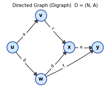 A digraph \(D = (N, A)\) with five nodes and six directed arcs. Each arc points from tail to head.
The out-degree of node \(v\) is the number of arcs leaving \(v\); the in-degree is the number arriving. A di-walk is a sequence of nodes \(v_0, \ldots, v_k\) where each \(v_i v_{i+1} \in A\). A di-path has no repeated nodes; a di-cycle is a closed di-walk with no repeated internal nodes.
The notion of a cut extends naturally to directed graphs, distinguishing between arcs going “forward” across the partition and arcs going “backward.”
The forward cut \(\delta(S)\) is what flow must traverse to get from \(S\) to its complement; the capacity of \(\delta(S)\) bounds how much flow can reach \(t\) from \(s\). This is the combinatorial content of max-flow min-cut.
(\(\Leftarrow\)) Let \(S\) be the set of all nodes reachable from \(s\) by a di-path. If \(t \in S\), we are done. Otherwise \(\delta(S)\) is an s,t-cut which, by assumption, is non-empty. Any arc \(uv \in \delta(S)\) with \(u \in S\) leads to \(v \notin S\) reachable from \(s\) — contradicting the definition of \(S\). \(\square\)
The proof uses the “reachability set” \(S\) — the set of all nodes reachable from \(s\). If the target \(t\) is not reachable, then \(\delta(S)\) is an empty cut, contradicting the assumption. This reachability argument is the template for all max-flow proofs.
1.3 The Underlying Graph and Cycles in Digraphs
To apply results from undirected graph theory (spanning trees, connectivity) to directed graphs, we sometimes need to “forget” directions. The underlying graph is the result of this forgetting.
The underlying graph captures connectivity structure but loses directional information. A digraph is “connected” if its underlying graph is connected, and “strongly connected” if there are directed paths in both directions between every pair of nodes.
Definition 2.3.6 (Strongly Connected). A digraph \(D = (N, A)\) is strongly connected if for all \(s, t \in N\) there is both an s,t-dipath and a t,s-dipath.
Strong connectivity is strictly stronger than connectivity: a connected digraph has an undirected path between every pair of nodes, while a strongly connected digraph has a directed path in each direction.
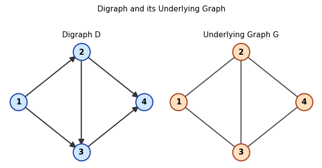 Left: digraph \(D\) with directed arcs. Right: its underlying graph \(G\) with directions removed.
A cycle in a digraph is a cycle in its underlying graph. Given an orientation of a cycle \(C\), arcs pointing in the direction of traversal are forward arcs and those opposing it are backward arcs. A digraph is connected if its underlying graph is connected, and strongly connected if every pair of nodes is mutually reachable via di-paths.
Spanning trees of digraphs will be essential as bases for the network simplex method: a spanning tree on \(n\) nodes has exactly \(n-1\) arcs and, crucially, admits a unique path between every pair of nodes in the underlying graph. This uniqueness of paths within a tree is precisely why tree bases support efficient computation in the simplex method.
1.4 Node-Arc Incidence Matrix
The node-arc incidence matrix is the algebraic encoding of a digraph — the bridge between combinatorics and linear algebra. It will be the constraint matrix of the transshipment LP, and its structure will explain why spanning trees are bases.
Each column of \(M\) corresponds to one arc, with a \(-1\) at the tail and a \(+1\) at the head. The product \(Mx = b\) encodes the flow conservation constraints: the net flow into node \(v\) (in-arcs minus out-arcs) equals the demand \(b_v\).
Every column of \(M\) has exactly one \(+1\) and one \(-1\). Summing all rows gives the zero vector, so the rows are linearly dependent and \(\text{rank}(M) \leq |N| - 1\). When \(D\) is connected, the rank is exactly \(|N| - 1\).
Key propositions on linear dependence:
The following propositions establish the fundamental link between linear algebra (bases of \(M\)) and combinatorics (spanning trees). This link is what allows the simplex method to be “network-flavored.”
The proof reorients arcs to form a “clean” directed cycle, making the linear dependence visually obvious: the sum telescopes to zero. This is why cycles and linear dependence are synonymous in the incidence matrix.
The converse — dependence implies cycle — is proved by showing that a cycle-free set (a forest) has linearly independent columns via a leaf-removal argument.
Together these propositions give the fundamental theorem that makes the network simplex method algebraically coherent:
This theorem is the reason the network simplex method uses spanning trees as bases: the simplex basis is precisely the spanning tree, and moving from one basis to another is precisely the tree exchange operation (enter one arc, leave another).
Chapter 2: The Transshipment Problem
The transshipment problem (TP) is the simplest and most fundamental network flow model. Imagine a set of depots (some with surplus goods, some with deficit) connected by a road network. We want to route goods at minimum cost to satisfy all demands. This chapter develops the LP formulation, its dual, and the network simplex algorithm — a geometrically beautiful specialization of the simplex method exploiting the tree structure of bases.
2.1 Problem Formulation
Let \(D = (N, A)\) be a connected digraph, \(b \in \mathbb{R}^N\) be node demands (where \(b_v > 0\) means node \(v\) supplies \(b_v\) units and \(b_v < 0\) means it demands \(|b_v|\) units), and \(w \in \mathbb{R}^A\) be arc costs. We assume \(\sum_{v \in N} b_v = 0\) (total supply equals total demand).
A flow is a vector \(x \in \mathbb{R}^A\) satisfying flow conservation at every node: inflow minus outflow equals the demand.
The LP formulation writes flow conservation at every node as a linear equality, with arc costs forming the objective.
The matrix form \(Mx = b, x \geq 0\) is an LP in Standard Equality Form. Since \(M\) is the node-arc incidence matrix, its bases are spanning trees — and this is what gives the transshipment problem its beautiful combinatorial structure.
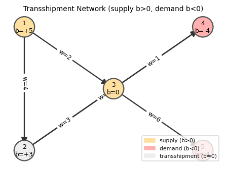 A transshipment network. Nodes with \(b > 0\) (yellow) are suppliers; nodes with \(b < 0\) (red) are consumers; \(b = 0\) nodes (grey) are pure transit points.
2.2 Dual LP and Complementary Slackness
Every LP has a dual. For the transshipment problem, the dual has a beautiful economic interpretation — node potentials represent “prices” — and gives the complementary slackness conditions that the network simplex algorithm maintains and checks at each step.
The dual of the TP has one variable \(y_v\) for each node \(v\):
\[\max\; y^T b \quad \text{s.t.} \quad y_v - y_u \leq w_{uv}\;\;\forall uv \in A,\quad y \text{ free}.\]Since the primal constraints are equalities, the dual variables are free (unconstrained). The dual is interpreted as a node potential: imagine \(y_v\) as the “price” of goods at node \(v\).
Think of what it means for a commodity market to be in equilibrium. If the price of grain at city \(u\) is \(y_u\) and the price at city \(v\) is \(y_v\), then a trader who buys at \(u\), pays shipping cost \(w_{uv}\), and sells at \(v\) earns a net profit of \(y_v - y_u - w_{uv}\). In a perfectly competitive market at equilibrium, no trade is strictly profitable — all arbitrage opportunities have been exhausted. This economic picture is exactly what a node potential captures, and it is also the dual feasibility condition for the transshipment LP. The three definitions below make this precise.
Definition 3.4.1 (Node Potential). A vector \(y \in \mathbb{R}^N\) is called a node potential.
A node potential is simply a price system: one number per node, with no constraint yet. Any vector qualifies as a potential; the interesting question is what constraints make it “dual feasible” and what makes it “certify optimality.”
Definition 3.4.2 (Reduced Cost). Given a node potential \(y \in \mathbb{R}^N\), the reduced cost of arc \(uv\) is \(\bar{w}_{uv} := w_{uv} + y_u - y_v\).
The reduced cost measures the “profitability” of using arc \(uv\): it is the cost of shipping one unit from \(u\) to \(v\) after accounting for the change in node prices. A negative reduced cost indicates a profitable shipping route — the trader makes money — while a positive reduced cost means the route loses money at the current price system. Crucially, the reduced cost depends on the price system \(y\), not just on the arc cost \(w_{uv}\). This is the key algebraic miracle of LP duality for networks: by choosing \(y\) cleverly (specifically, by setting \(y_v = 0\) at a root and propagating via tree arcs), we get reduced costs that reveal exactly which arcs to enter or leave in the simplex pivot.
Definition 3.4.3 (Feasible Potential). A node potential \(y\) is feasible if \(\bar{w}_{uv} \geq 0\) for all arcs \(uv \in A\).
Feasibility of the potential is the dual feasibility condition: no arc has a “profitable” reduced cost. Economically, it means the price system is at equilibrium — no trader can profit by routing goods along any arc. When the potential is feasible and satisfies the complementary slackness conditions with a primal flow \(x\), the pair \((x, y)\) is simultaneously optimal by LP strong duality. The network simplex algorithm is precisely the process of searching for such a matching pair: start with a feasible tree flow, construct the unique feasible potential for that tree, and pivot until all non-tree arcs have non-negative reduced costs.
The key optimality condition follows immediately from LP complementary slackness theory:
Complementary slackness is the “on/off” condition: each arc either carries zero flow (it’s not worth using) or has zero reduced cost (it’s exactly break-even). No arc is used at positive flow unless it is cost-optimal given the current prices.
Economic interpretation: The reduced cost \(\bar{w}_{uv} = w_{uv} + y_u - y_v\) represents the net cost of buying one unit at \(u\) for price \(y_u\), shipping it at cost \(w_{uv}\), and selling at \(v\) for price \(y_v\). If \(\bar{w}_{uv} > 0\), shipping through \(uv\) is unprofitable, so we never use it (\(x_{uv} = 0\)). If \(\bar{w}_{uv} < 0\), it is profitable, so we want as much flow as possible through it.
2.3 Bases are Spanning Trees
A fundamental structural theorem links LP bases for the TP to combinatorial objects:
A tree flow (basic feasible solution) is determined by a spanning tree \(T\): we set non-tree arcs to zero and solve for the tree arc flows iteratively from the leaves inward. At each leaf \(v\) of \(T\), exactly one arc is incident, so its flow is forced to be \(b_v\).
The tree flow is the combinatorial analogue of a basic feasible solution: it is the unique way to route flow through a spanning tree that satisfies all node demands.
The tree flow is computed iteratively from the leaves inward: at each leaf, there is exactly one tree arc incident to it, so the flow on that arc is uniquely determined by the demand. Peeling leaves one by one determines the entire tree flow.
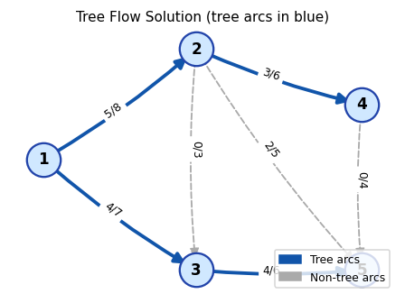 A tree flow: bold blue arcs form the spanning tree \(T\), and dashed grey arcs are non-tree arcs with flow 0. Labels show flow/capacity.
Note: Not every spanning tree yields a feasible flow. For a tree to give a basic feasible solution, the iterative leaf-deletion computation must produce non-negative flows on all tree arcs.
2.4 Network Simplex Algorithm for the TP
The network simplex method applies the simplex algorithm to the TP, exploiting the tree-basis structure at every step.
Maintaining the dual: For a given spanning tree \(T\), we compute potentials \(y\) by setting \(y_{\text{root}} = 0\) for some fixed root node and propagating via \(\bar{w}_{uv} = 0\) for all tree arcs \(uv\): i.e., \(y_v = y_u + w_{uv}\) if \(uv \in T\) (or \(y_v = y_u - w_{vu}\) if \(vu \in T\)).
Finding an entering arc: Compute \(\bar{w}_{uv}\) for all non-tree arcs. If any \(\bar{w}_{uv} < 0\), the solution is not optimal; that arc enters the basis.
Finding a leaving arc: Adding \(uv\) to \(T\) creates exactly one cycle \(C\). Orient \(C\) so that \(uv\) is a forward arc. Increasing flow by \(t\) on \(uv\) requires adding \(t\) to all forward arcs of \(C\) and subtracting \(t\) from all backward arcs. The maximum feasible increase is \(t = \min\{x_{pq} : pq \text{ backward in } C\}\). The backward arc attaining this minimum leaves the basis: \(T \leftarrow T + uv - pq\).
Network Simplex Algorithm for TP
─────────────────────────────────
Input:  Connected digraph D=(N,A), arc costs w, node demands b,
        initial spanning tree T with feasible tree flow x.
1. Compute node potentials y: set y_root = 0, then for each
   arc uv in T set y_v = y_u + w_uv (or y_v = y_u - w_vu).
2. For each non-tree arc uv, compute w̄_uv = w_uv + y_u - y_v.
3. While ∃ non-tree arc uv with w̄_uv < 0:
   a. T + uv forms a unique cycle C;
      orient C so uv is a forward arc.
   b. Let t = min{x_pq : pq backward arc of C}.
      Let pq attain this minimum.
   c. x_e += t for forward arcs of C;
      x_e -= t for backward arcs of C.
   d. T ← T + uv - pq.
   e. Recompute potentials and reduced costs. Go to 3.
4. Return x (optimal tree flow).
2.5 Economic Interpretation of Dual Potentials
Node potentials have a natural economic interpretation. Think of \(y_v\) as the market price of a commodity at node \(v\). The reduced cost \(\bar{w}_{uv} = w_{uv} + y_u - y_v\) is the profit/loss from buying one unit at \(u\), transporting it at cost \(w_{uv}\), and selling at \(v\):
- \(\bar{w}_{uv} > 0\): lose money — don’t ship (set \(x_{uv} = 0\)).
- \(\bar{w}_{uv} < 0\): make money — ship as much as possible.
- \(\bar{w}_{uv} = 0\): break even — any flow level is equally optimal.
2.6 Unboundedness
Most transshipment problems are bounded (finite optimal cost), but unboundedness can occur if there is a “money machine” in the network — a directed cycle where circulating flow generates negative cost.
The algorithm may fail to find a leaving arc when all backward arcs of the cycle \(C\) have zero flow — equivalently, the entering arc’s flow can increase without bound. This happens precisely when \(D\) contains a negative di-cycle.
A negative di-cycle is a cycle where the net cost of routing flow around it is negative — every unit of flow circulated around \(C\) reduces the total cost. Since flow can be circulated indefinitely, the problem is unbounded.
(\(\Rightarrow\)) If no leaving arc is found, the entering arc \(uv\) creates a cycle \(C\) with all forward arcs. The potentials along \(C\) sum to give \(\bar{w}_{uv} = \sum_{e \in C} w_e < 0\), so \(C\) is a negative di-cycle. \(\square\)
The proof in the (\(\Leftarrow\)) direction constructs the unbounded direction explicitly: add a circulation along the negative cycle. The (\(\Rightarrow\)) direction shows the simplex algorithm “discovers” the negative cycle when no leaving arc exists.
2.7 Finding an Initial BFS
To start the simplex algorithm we need a feasible tree flow. The standard technique introduces an auxiliary digraph.
The auxiliary TP has a natural feasible flow: route all supply through \(z\) and out to demand nodes. This flow is the initial BFS.
2.8 Feasibility Characterization
since \(\delta(S) = \emptyset\). But \(x \geq 0\) implies \(x(\delta(\bar{S})) \geq 0\) — contradiction. \(\square\)
Chapter 3: Minimum-Cost Flow
The transshipment problem of Chapter 2 allows unlimited flow on any arc — an unrealistic assumption for most applications. Adding capacity constraints transforms it into the minimum-cost flow problem, which is both more realistic and more widely applicable. Remarkably, the network simplex algorithm extends with only minor modifications.
The minimum-cost flow problem (MCFP) generalizes the transshipment problem by adding capacity constraints: each arc \(e\) can carry at most \(c_e\) units of flow. This single addition dramatically widens the modeling power — airline scheduling, catering logistics, bipartite matching, and matrix rounding all reduce to MCFP instances.
3.1 LP Formulation and Its Dual
The MCFP adds upper bounds on each arc flow. The LP formulation is nearly identical to the TP, with the addition of the capacity constraints.
The capacity constraints \(x_e \leq c_e\) transform the TP into the MCFP. Each arc can no longer carry unlimited flow — there is a physical or contractual limit. This makes the problem more realistic and, through the CS conditions, introduces a richer set of optimality conditions.
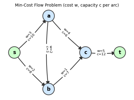 An MCFP instance: each arc is labeled with its cost \(w\) and capacity \(c\). We seek a flow satisfying demands at minimum total cost.
We introduce slack variables \(s_e = c_e - x_e \geq 0\) for each arc, converting the upper-bound constraints to equalities. The augmented LP has the dual:
\[\max\; b^T y - c^T z \quad \text{s.t.} \quad -y_u + y_v - z_{uv} \leq w_{uv},\quad z \geq 0.\]The reduced cost takes the same form as before: \(\bar{w}_{uv} = w_{uv} + y_u - y_v\). The dual constraint rewrites as \(z_{uv} \geq -\bar{w}_{uv}\), and since we minimize \(c^T z\) (with \(c > 0\)), the optimal \(z\) satisfies \(z_{uv} = \max\{0, -\bar{w}_{uv}\}\). Complementary slackness then yields:
The complementary slackness conditions for MCFP are richer than for TP, because now arcs can be at three “states”: zero, saturated at capacity, or strictly interior.
- \(\bar{w}_{uv} < 0 \Rightarrow x_{uv} = c_{uv}\)
- \(\bar{w}_{uv} > 0 \Rightarrow x_{uv} = 0\)
- \(0 < x_{uv} < c_{uv} \Rightarrow \bar{w}_{uv} = 0\)
Economic interpretation: If the reduced cost is negative, shipping through that arc is profitable, so saturate it; if positive, unprofitable, so use it not at all; if zero, any intermediate flow level is equally optimal. These three cases directly drive the network simplex: an arc violates CS if it has negative reduced cost at zero flow (should increase) or positive reduced cost at capacity (should decrease).
Note that MCFP cannot be unbounded since capacities \(c_e\) provide an upper bound on total flow.
3.2 Basis Structure for MCFP
The augmented matrix of the MCFP LP has rank \(|N| - 1 + |A|\), so a basis has exactly \(|N| + |A| - 1\) elements. Each arc \(e\) contributes either \(x_e\) alone, \(s_e\) alone, or both to the basis:
- Case 1 (\(s_e\) in basis, \(x_e\) not): \(x_e = 0\).
- Case 2 (\(x_e\) in basis, \(s_e\) not): \(x_e = c_e\) (arc saturated).
- Case 3 (both in basis): arc carries an intermediate flow level.
By counting — let \(k\) be the number of Case 3 arcs — there are \(2k + |A| - k = k + |A|\) basic variables total, which must equal \(|N| + |A| - 1\), giving \(k = |N| - 1\). These \(|N|-1\) arcs form a spanning tree (by the same cycle argument as for TP). The remaining arcs in Cases 1 and 2 are fixed at 0 or \(c_e\).
3.3 Network Simplex for MCFP
The network simplex for MCFP extends the TP version by handling both “free” and “saturated” non-tree arcs. We search for a violating arc:
- A non-tree arc \(e\) with \(\bar{w}_e < 0\) and \(x_e = 0\) (should be increased to \(c_e\)), or
- A non-tree arc \(e\) with \(\bar{w}_e > 0\) and \(x_e = c_e\) (should be decreased to 0).
In either case, adding \(e\) to \(T\) creates a cycle. We push flow around the cycle, respecting both \(x \geq 0\) and \(x \leq c\). The amount pushed is \(t = \min\bigl(\{c_f - x_f : f \text{ forward arc of } C\},\; \{x_f : f \text{ backward arc of } C\}\bigr)\). The leaving arc is the one that first reaches 0 or \(c_e\).
Network Simplex Algorithm for MCFP
────────────────────────────────────
Input:  D=(N,A), costs w, capacities c, demands b,
        initial spanning tree T with tree flow x (non-tree arcs at 0 or c_e).
1. Compute potentials y from T (same as TP).
2. Compute w̄_e for all non-tree arcs e.
3. While ∃ violating arc e = uv:
   Case A: w̄_e < 0 and x_e = 0 → orient C so e is a forward arc.
   Case B: w̄_e > 0 and x_e = c_e → orient C so e is a backward arc.
   a. t = min({c_f - x_f : f forward}, {x_f : f backward})
   b. Let f be the arc attaining t.
   c. Update flows along C (add t to forward, subtract from backward).
   d. T ← T + e - f.  Recompute potentials and reduced costs.
4. Return x (optimal flow).
3.4 Integrality of MCFP
One of the most practically important properties of network flow problems: integer inputs yield integer outputs. This means integer programming formulations of scheduling, matching, and routing problems can be solved as (polynomial-time) LPs.
The proof exploits the fact that the network simplex updates flow by integer amounts: the entering flow \(t\) is a minimum over integers, hence an integer. This integrality flows through every iteration, preserving the integer structure from start to finish. Algebraically, this follows because the node-arc incidence matrix is totally unimodular — all bases have determinant \(\pm 1\) — so Cramer’s rule always produces integer basic solutions from integer data.
3.5 Feasibility of MCFP
Use the same auxiliary digraph as for the TP, but the new arcs have infinite capacity (or a large finite bound). The feasibility characterization is:
3.6 Applications
Minimum Bipartite Perfect Matching. Given a bipartite graph \(G = (A \cup B, E)\) with \(|A| = |B|\) and edge costs, we want a minimum-cost perfect matching. Model as MCFP: direct each edge from \(A\) to \(B\); set \(b_v = -1\) for \(v \in A\), \(b_v = +1\) for \(v \in B\); set all capacities to 1. By integrality, the optimal solution has \(x_e \in \{0,1\}\), giving exactly a perfect matching.
Airline Scheduling. A plane visits cities \(1, \ldots, n\). There are \(b_{ij}\) potential passengers from city \(i\) to \(j\) (\(i < j\)), ticket price \(f_{ij}\), and plane capacity \(P\). Model:
- Nodes \(1, \ldots, n\) with arcs along the route for the plane (capacity \(P\), cost 0).
- For each passenger group \((i,j)\), a node with demand \(-b_{ij}\) connected to the plane route at city \(i\) and to a sink at city \(j\) with arc cost \(-f_{ij}\) (negative = revenue). The minimum-cost flow assigns passengers to the plane or leaves them unserved.
Catering Problem. A caterer needs \(b_i\) clean napkins each day \(i = 1, \ldots, n\). New napkins cost \(\alpha\); used napkins can be returned via 1-day service (cost \(\beta\)) or 2-day service (cost \(\gamma\)); storage is free. Model each day as a node, dirty napkins as supply, clean napkins as demand, and the three treatment options as arcs connecting “dirty” nodes to “clean” nodes on the appropriate day. The minimum-cost flow gives the optimal napkin procurement strategy.
Matrix with Consecutive 1’s. The LP \(\min w^T x\) s.t. \(Ax \geq b\), \(x \geq 0\), where each column of \(A\) has a contiguous block of 1’s, can be transformed via successive row operations (subtracting adjacent rows) into an incidence matrix LP — hence it reduces to an MCFP and can be solved by network simplex.
Example 4.5.2. A manufacturing company must contract for \(d(i)\) units of storage for time periods \(i = 1, \ldots, n\). Let \(w_{ij}\) denote the cost of 1 unit of storage capacity acquired at the beginning of period \(i\) and held through period \([i, j)\). The problem of deciding how much capacity to acquire, at what times, and for how many periods reduces to the matrix-with-consecutive-1’s LP above and can be solved as an MCFP.
Chapter 4: Shortest Paths
The transshipment and minimum-cost flow problems are rich and general, but the most classical network problem — finding the shortest path between two nodes — deserves its own dedicated analysis. The LP duality perspective from Chapters 2 and 3 applies here too: dual potentials are exactly shortest distances, and the CS conditions reduce to “no arc has negative reduced cost.” This perspective unifies all three algorithms (Ford, Bellman-Ford, Dijkstra) into a single framework.
Although the network simplex can solve shortest path problems as a special case of the TP, it is not polynomial-time. Dedicated shortest-path algorithms exploit the special structure to achieve much better efficiency. This chapter develops three algorithms — Ford’s (general), Bellman-Ford (handles negative costs, detects negative cycles), and Dijkstra’s (fast for non-negative costs) — together with a rigorous LP-duality perspective.
4.1 Problem and LP Formulation
The shortest path problem is the simplest nontrivial special case of the TP: one unit of flow must travel from \(s\) to \(t\) at minimum cost.
Example 5.1.1. Consider a digraph with nodes \(\{s, a, b, t\}\) and arcs \(sa\) (cost 2), \(ab\) (cost \(-4\)), \(bt\) (cost 5), \(sb\) (cost 2), \(at\) (cost \(-1\)). The shortest s,t-dipath is found by testing all paths: \(s \to a \to b \to t\) has cost \(2 + (-4) + 5 = 3\); \(s \to a \to t\) has cost \(2 + (-1) = 1\); \(s \to b \to t\) has cost \(2 + 5 = 7\). The shortest path is \(s \to a \to t\) with total cost 1.
The characteristic vector encodes which arcs are used in a path. Any integral feasible solution to the LP corresponds to a combination of characteristic vectors of paths and cycles. The LP formulation treats the shortest path as a special TP with \(b_s = -1\), \(b_t = +1\), \(b_v = 0\) otherwise:
\[\min\; w^T x \quad \text{s.t.} \quad x(\delta(\bar{v})) - x(\delta(v)) = b_v\;\forall v,\quad x \geq 0.\]The dual is \(\max\; y_t - y_s\) subject to \(y_v - y_u \leq w_{uv}\) for all \(uv \in A\), where \(\bar{w}_{uv} = w_{uv} + y_u - y_v \geq 0\) is the dual feasibility condition.
Definition 5.4.1 (Equality Arc). Given a node potential \(y\), arc \(uv\) is an equality arc if \(\bar{w}_{uv} = w_{uv} + y_u - y_v = 0\).
Equality arcs are arcs that lie on a shortest path: the reduced cost is zero, meaning shipping one unit along such an arc is exactly break-even given the current prices. The CS conditions say that a path is optimal if and only if all of its arcs are equality arcs.
This gives a beautifully geometric picture of what a shortest path algorithm is doing from the LP perspective: it is gradually building up the set of equality arcs until these arcs contain a complete s,t-dipath. Each “relaxation” step in Bellman-Ford or Dijkstra turns one arc into an equality arc, enriching the equality-arc graph until the optimality certificate is complete.
Key theorem on LP structure:
An integral feasible solution to the shortest path LP need not itself be a dipath, as shown by the following example.
Example 5.3.1. Consider a digraph with nodes \(\{s, a, b, c, t\}\) where arcs \(sa\), \(sb\), \(at\), \(bc\), \(ca\) all carry positive flow. An integral feasible solution might route one unit from \(s\) along \(s \to a \to t\) (a dipath) plus one unit circulating around \(a \to \cdots \to a\) (a di-cycle). The LP solution is a sum of a dipath characteristic vector and a di-cycle characteristic vector, but is not itself a single dipath.
Theorem 5.3.2. If \(\bar{x}\) is an integral feasible solution to the shortest s,t-dipath LP, then \(\bar{x}\) is a sum of the characteristic vector of an s,t-dipath and the characteristic vectors of a collection of di-cycles.
Theorem 5.3.3. If there are no negative di-cycles, then the shortest s,t-dipath LP has an optimal solution that is the characteristic vector of a shortest s,t-dipath.
Theorems 5.3.2 and 5.3.3 together say that the LP perspective and the combinatorial perspective are fully consistent: even though the LP might in principle produce fractional or “multi-path” solutions, the absence of negative di-cycles guarantees that a clean single-dipath optimal solution always exists. This is reassuring for the algorithmic perspective — it means any algorithm that finds the LP optimal value also finds an actual shortest path, not just an abstract flow decomposition.
4.2 Shortest Path Trees and Subpath Optimality
When shortest paths are well-defined (no negative di-cycles), they have a beautiful recursive structure: every subpath of a shortest path is itself shortest. This “subpath optimality” or “Bellman’s principle of optimality” is the key property exploited by all efficient shortest path algorithms.
A shortest path tree organizes all shortest paths from a single source \(s\) into a single spanning tree structure. Every branch of the tree is a shortest path to the node at its leaf.
This characterization makes rooted spanning trees easy to check algorithmically: verify in-degrees. The single-predecessor structure means each node has exactly one “parent” on its shortest path back to \(s\).
The proof uses the LP dual \(y\) as a certificate: the optimal potentials for the full path \(P\) also certify optimality for every subpath, by the CS conditions. This “dual certificate transfers to subproblems” argument is elegant and reveals why LP duality is the right lens for shortest paths.
4.3 Ford’s Algorithm (General Framework)
All three shortest-path algorithms share a common structure: maintain a vector of tentative distances \(y\), and iteratively “correct” arcs with negative reduced cost. Ford’s algorithm is the most general formulation of this idea — it handles arbitrary arc costs (including negative ones) and terminates correctly when no negative cycles exist.
Ford’s algorithm is a general iterative scheme applicable even with negative arc costs.
Ford's Algorithm
──────────────────
Input:  D=(N,A), arc costs w, source s.
        (Assume all nodes reachable from s.)
1. Set y_s = 0, y_v = ∞ for all v ≠ s.
   Set predecessor p_v = ∅ for all v.
2. While ∃ arc uv with w̄_uv = w_uv + y_u - y_v < 0:
   a. y_v ← y_u + w_uv.   ("correct" the arc uv)
   b. p_v ← u.
3. Return y (shortest distances) and D_p (shortest-path tree).
Key properties:
The following propositions establish correctness of Ford’s algorithm — the predecessor digraph \(D_p\) always encodes valid shortest paths, and termination implies optimality.
Proposition 5.6.1. Throughout Ford’s algorithm, \(\bar{w}_e \leq 0\) for all arcs \(e \in A(D_p)\).
Non-positive reduced costs on predecessor arcs means the predecessor digraph always provides valid “equality arc” paths — the template for CS optimality.
Propositions 5.6.2 and 5.6.3 together identify the two ways Ford’s algorithm can “detect” a negative di-cycle: either the predecessor digraph wraps around into a cycle, or the source \(s\) itself acquires a predecessor (meaning there is a cycle back to the start). Both cases are signatures of a negative cycle and both imply the algorithm cannot terminate — every time it tries to settle, there is another profitable correction to make.
Proposition 5.6.2. If \(D_p\) contains a di-cycle at any point, then \(D\) contains a negative di-cycle and the algorithm does not terminate.
Proposition 5.6.3. If \(s\) acquires a predecessor at any point, then \(D\) contains a negative di-cycle and the algorithm does not terminate.
These propositions make Ford’s algorithm a negative cycle detector as well as a shortest path solver: if it does not terminate, it has found a negative di-cycle.
Propositions 5.6.2 and 5.6.3 form a beautiful duality of their own: Ford’s algorithm either certifies optimality (termination with a valid shortest-path tree) or certifies infeasibility-of-optimality (non-termination, with a negative cycle as witness). There is no third outcome. Proposition 5.6.4 makes the positive case precise.
Proposition 5.6.4. If Ford’s algorithm terminates, then \(D_p\) is a spanning tree of shortest dipaths rooted at \(s\), and \(y_v = d(s,v)\) for all \(v\).
The proof invokes LP strong duality: at termination, the primal (the shortest path) and dual (the potentials \(y\)) satisfy complementary slackness, so both are optimal. This is the LP duality proof of correctness for shortest path algorithms.
4.4 Bellman-Ford Algorithm
Ford’s algorithm is correct but unspecified about the order of arc corrections, which may lead to exponential running time. Bellman-Ford provides a specific schedule — scan all arcs in \(|N|-1\) passes — that guarantees polynomial termination and detects negative cycles in a final pass.
Here is the critical question that motivates two separate algorithms rather than one: what if arc costs can be negative? In many real-world problems — currency exchange, pipeline networks with revenue arcs, resource arbitrage — negative costs are natural. Dijkstra’s algorithm, which we meet shortly, is extraordinarily fast but requires non-negative arc costs for its greedy invariant to work. Bellman-Ford makes no such assumption: it handles arbitrary costs, detecting negative cycles as a bonus. The price is a slower running time of \(O(|N| \cdot |A|)\), versus Dijkstra’s near-linear \(O(|N| \log |N| + |A|)\). Understanding why this trade-off exists is the key insight of Chapter 4: Dijkstra’s greedy strategy works because once a node is “settled” under non-negative costs, no future path can improve it. With negative costs, a later arc might make a previously-settled node cheaper, so we cannot settle nodes greedily — we must keep revising. Bellman-Ford’s genius is recognizing that any shortest path visits at most \(|N|-1\) arcs (otherwise it would contain a cycle, and if there are no negative cycles, such cycles can be stripped away without increasing path cost). So \(|N|-1\) passes through all arcs is always enough.
Bellman-Ford makes Ford’s algorithm efficient by scanning all arcs in passes.
Bellman-Ford Algorithm
──────────────────────
Input:  D=(N,A), arc costs w, source s.
1. y_s = 0, y_v = ∞ for v ≠ s; p_v = ∅; i = 0.
2. While i < |N| - 1:
   a. For each arc uv ∈ A:
      if w̄_uv < 0 then y_v ← y_u + w_uv; p_v ← u.
   b. i ← i + 1.
3. If any w̄_uv < 0 remains: D has a negative di-cycle.
   Else: y_v = d(s,v) for all v reachable from s.
Running time: \(O(|N| \cdot |A|)\).
The following theorem shows that Bellman-Ford correctly computes all shortest paths in \(|N|-1\) passes when no negative cycles are present. The proof proceeds in two stages: first establish that the algorithm’s estimates are always optimistic (never below the true distance), and then show that after exactly \(i\) passes, the estimate for any node whose shortest path uses \(i\) arcs has converged to the truth. Together these two facts pinch the estimates to the correct value from both directions.
Proposition 5.7.2. Suppose no negative di-cycles exist. At any point in Ford’s or Bellman-Ford’s algorithm, \(y_v \geq d(s,v)\) for all \(v\).
This lower bound is the key invariant: the algorithm’s estimates never go below the true shortest distance. The following theorem shows the estimates converge from above:
Proposition 5.7.2 gives the lower bound: estimates can never underestimate true distances. The following theorem closes the gap from above, showing that after exactly \(i\) passes, every node whose shortest path uses \(i\) arcs or fewer has converged to its true distance. Together these two facts pinch the estimates to the exact correct value — a proof strategy sometimes called the “sandwich argument.”
Theorem 5.7.1 (Bellman-Ford Correctness). Suppose no negative di-cycles exist. After the \(i\)-th pass of Bellman-Ford, if the shortest s,v-dipath uses at most \(i\) arcs, then \(y_v = d(s,v)\).
First note that at any point, \(y_v \geq d_v\): at initialization \(\infty \geq d_v\); when \(y_v \neq \infty\), trace \(v\) back to \(s\) in \(D_p\). Since \(\bar{w}_e \leq 0\) for all \(e \in D_p\), summing gives \(w(P) - y_v \leq 0\) so \(y_v \geq w(P) \geq d_v\).
Base case \(i = 0\): trivial. Inductive step: pick \(v\) with a shortest path using at most \(i+1\) arcs \(s = v_0, v_1, \ldots, v_{i+1} = v\). By subpath optimality and induction, \(y_{v_i} = d_{v_i}\) after pass \(i\). In pass \(i+1\):
- If \(\bar{w}_{v_i v} = 0\): already \(y_v = y_{v_i} + w_{v_i v} = d_v\) and doesn’t change.
- If \(\bar{w}_{v_i v} > 0\): then \(y_v < d_v\) — contradicts the lemma.
- If \(\bar{w}_{v_i v} < 0\): the algorithm corrects and sets \(y_v = y_{v_i} + w_{v_i v} = d_v\). \(\square\)
Corollary 5.7.2.1. At the end of Bellman-Ford: if \(y\) is feasible, then \(y_v = d(s,v)\) for all \(v\). If \(y\) is not feasible, a negative di-cycle exists.
The corollary is Bellman-Ford’s clean termination guarantee: run \(|N|-1\) passes, then do one final pass as a check. If any arc still has a negative reduced cost, you have certified the existence of a negative di-cycle — the algorithm doubles as a cycle detector. If no such arc remains, the distance labels are exact shortest distances. This two-in-one capability makes Bellman-Ford indispensable in practice even though Dijkstra is faster when costs are non-negative.
Application — Currency Exchange: Given currencies with exchange rates \(r_{uv}\), a profitable cycle exists iff \(\prod_{e \in C} r_e > 1\), i.e., \(\sum_{e \in C} (-\log r_e) < 0\). Set arc costs to \(-\log r_e\) and run Bellman-Ford to detect a negative di-cycle.
Notice what makes the currency-exchange application work: the problem is non-linear (products instead of sums), but the logarithm transformation converts it into an additive shortest-path problem with potentially negative costs. This is precisely the setting where Bellman-Ford shines and Dijkstra cannot be applied. The choice of algorithm is dictated by the sign structure of the costs, and this is a theme that recurs throughout applied optimization: understanding what structural assumption an algorithm requires is as important as knowing how fast it runs.
4.5 Dijkstra’s Algorithm
Bellman-Ford’s \(O(|N| \cdot |A|)\) running time is acceptable for general arc costs, but when all costs are non-negative, we can do far better. Non-negativity allows a greedy approach: once a node is “settled” (its shortest distance determined), it never needs to be reconsidered. This greedy invariant is the core of Dijkstra’s algorithm.
Let us be precise about why non-negativity unlocks a greedy approach that Bellman-Ford cannot use. With \(w \geq 0\), any path that leaves the “settled” set \(T\) and later returns to it must travel through at least one additional non-negative arc, making it at least as long as paths that stay within \(T\). So once we have determined the shortest distance to a node \(v\), no extension of any path leaving \(v\) can return and offer a better route to an already-settled node. This greedy monotonicity is the entire reason Dijkstra is correct: we always settle the node with the smallest current estimate, and that estimate is already final. The LP interpretation is beautiful: at each step, we raise the dual potential \(y_v\) for all unsettled nodes by the minimum reduced cost \(\bar{w}_{uv}\) for any arc leaving the settled set, making exactly one arc an equality arc and settling one more node. We maintain dual feasibility throughout, and at termination, all nodes are settled and \(y_v = d(s,v)\).
When all arc costs are non-negative, we can exploit a greedy strategy: raise the potentials of unsettled nodes by \(t\) at each step while maintaining feasibility.
Motivation: With \(w \geq 0\), setting \(y = 0\) is a feasible dual potential. We maintain feasibility by carefully choosing how much to raise potentials. For an arc \(uv\) with \(u\) settled and \(v\) unsettled, the reduced cost \(\bar{w}_{uv}\) decreases as \(y_v\) increases. We pick the arc \(uv \in \delta(N(T))\) with minimum \(\bar{w}_{uv}\) and raise all unsettled potentials by \(\bar{w}_{uv}\), making \(uv\) an equality arc. Adding \(v\) to the tree settles it permanently.
Dijkstra's Algorithm
──────────────────────
Input:  D=(N,A), non-negative costs w ≥ 0, source s.
1. Initialize y_v = 0 for all v; T = {s} (settled set).
2. While T is not a spanning tree of N:
   a. Find arc uv ∈ δ(N(T)) minimizing w̄_uv = w_uv + y_u - y_v.
   b. Set y_z ← y_z + w̄_uv for all z ∉ N(T).
   c. Add arc uv and node v to T (settle v).
3. Output y_v = d(s,v) for all v.
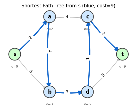 A shortest path tree (blue arcs) found by Dijkstra’s algorithm. Grey arcs were not selected. Node labels show the optimal distance from s.
 Animation: Dijkstra’s algorithm. Green nodes are settled (permanently optimized), blue nodes are unsettled. The frontier expands one node at a time.
Correctness: The four cases for how \(\bar{w}_{uv}\) changes when we increment \(y_z\) for \(z \notin N(T)\):
- Both \(u, v \notin N(T)\): both increase by \(t\), so \(\bar{w}_{uv}\) unchanged.
- Both \(u, v \in N(T)\): neither changes, \(\bar{w}_{uv}\) unchanged.
- \(u \notin N(T)\), \(v \in N(T)\): \(y_u\) increases, \(\bar{w}_{uv}\) increases — still feasible.
- \(u \in N(T)\), \(v \notin N(T)\): \(y_v\) increases, \(\bar{w}_{uv}\) decreases — the minimum such arc becomes an equality arc and is added to \(T\).
All arcs in \(T\) are equality arcs at all times, and \(y\) is always feasible. The LP argument then gives \(y_v = d(s,v)\) upon termination.
Running time: \(O(|N| \log |N| + |A|)\) with a Fibonacci heap.
Applications:
Proposition 5.9.1 (Network Reliability). Given a digraph \(D = (N, A)\) with arc reliabilities \(r_e \in (0, 1]\), modify Dijkstra’s algorithm to maximize reliability of an s,t-dipath by replacing addition with multiplication and minimum with maximum, or equivalently, minimize \(\sum_{e \in P}(-\log r_e)\) with \(-\log r_e \geq 0\) using the standard Dijkstra algorithm.
- Currency Exchange: To detect a profitable exchange cycle, use Bellman-Ford (negative di-cycle detection) with costs \(-\log r_e\).
Chapter 5: Maximum Flow and Min-Cut
Having studied cost-minimizing flows (Chapters 2–3) and distance-minimizing paths (Chapter 4), we now turn to volume-maximizing flows. Maximum flow asks: given a source \(s\) and sink \(t\) in a capacitated network, what is the greatest amount of material we can push from \(s\) to \(t\) without violating any capacity? The celebrated Max-Flow Min-Cut theorem provides a deep and beautiful answer: the maximum flow value always equals the minimum cut capacity. This min-max equality — primal maximum equals dual minimum — is a special case of LP strong duality and connects to König’s theorem, Menger’s theorem, and Hall’s theorem through a unified framework.
5.1 LP Formulation
The maximum flow problem seeks to maximize the “throughput” from source to sink while respecting all capacity constraints and flow conservation.
This is a special case of MCFP (set \(b_s = -f\), \(b_t = f\), all other \(b_v = 0\) and maximize \(f\)). The flow conservation constraints enforce that all intermediate nodes neither create nor destroy flow — they are pure transit points.
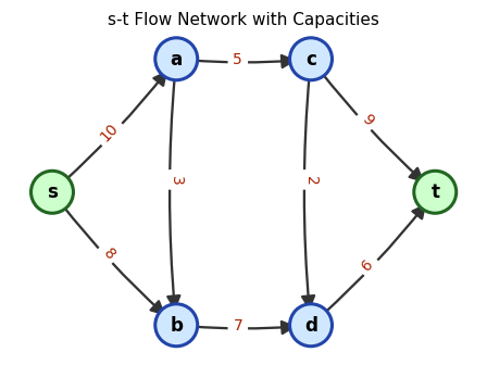 An s-t flow network with capacity labels on arcs. The source \(s\) (left) and sink \(t\) (right) are highlighted.
5.2 Residual Graph and Augmenting Paths
To find a maximum flow, we need a way to describe “where can we push more flow?” The residual graph answers this question by tracking remaining capacity on each arc and the possibility of “pulling back” flow on already-used arcs.
Given a flow \(x\), the residual graph \(D'\) captures where we can push additional flow:
- If \(x_{uv} < c_{uv}\): add forward arc \(uv\) to \(D'\) with residual capacity \(c_{uv} - x_{uv}\).
- If \(x_{uv} > 0\): add backward arc \(vu\) to \(D'\) with residual capacity \(x_{uv}\).
The backward arc \(vu\) in the residual graph represents the possibility of “canceling” existing flow on arc \(uv\). This is the mechanism that makes flow routing flexible: we are not committed to the current flow; we can reroute by adding backward residual arcs to augmenting paths.
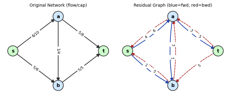 Left: a flow network with arc labels flow/capacity. Right: the residual graph — blue arcs are forward residuals, red dashed arcs are backward residuals.
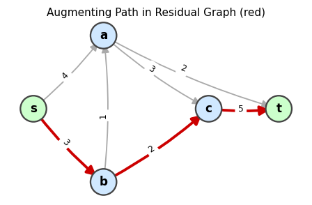 An augmenting path (red) in the residual graph. Pushing flow along this path increases the total flow.
5.3 Ford-Fulkerson Algorithm
Ford-Fulkerson Algorithm
──────────────────────────
Input:  Digraph D=(N,A), capacities c, source s, sink t.
1. Initialize x_e = 0 for all e ∈ A. Form residual graph D'.
2. While ∃ s,t-dipath (augmenting path) P in D':
   a. Let γ = min{residual capacity on P}.
   b. Augment x along P by γ:
      • Forward arcs: x_e += γ.
      • Backward arcs: x_e -= γ.
   c. Update D'.
3. Return x (maximum flow).
 Animation: Ford-Fulkerson on a 6-node network. Red arcs show the augmenting path at each iteration. Watch the flow labels update after each augmentation.
Termination:
- If \(c\) is integer-valued, each augmentation increases flow by at least 1, so the algorithm terminates.
- If \(c\) is rational, scale to integer capacities.
- If \(c\) is irrational, Ford-Fulkerson may cycle forever.
Even for integer capacities, the algorithm may require \(|f^*|\) iterations (pseudopolynomial). The Edmonds-Karp variant fixes this.
5.4 Edmonds-Karp: Shortest Augmenting Paths
If we always augment along the path with the fewest arcs (found by BFS), we obtain Edmonds-Karp. This single design decision — use BFS rather than arbitrary path-finding — transforms Ford-Fulkerson from a pseudopolynomial algorithm into a strongly polynomial one. The key intuition is this: if we always augment along shortest (fewest-arc) paths, we prevent the algorithm from “thrashing” back and forth along long routes. Instead, the BFS distances in the residual graph are monotonically non-decreasing, which means each arc can only become a bottleneck (critical) a bounded number of times before BFS distances to its endpoints increase. Once distances have increased enough, they can never decrease, and since distances are bounded by \(|N|\), the whole process terminates quickly.
The two lemmas below formalize this argument. The first establishes the monotone BFS distance property, which is the structural core of the bound. The second translates it into a count of critical arc events — the mechanism by which each iteration gets charged.
Lemma 6.3.1. Let \(d_f(s, v)\) denote the minimum number of arcs in an s,v-dipath in the residual graph \(D_f\). If \(f'\) is the flow after the next iteration of Edmonds-Karp, then \(d_f(s, v) \leq d_{f'}(s, v)\) for all \(v \in N\).
Lemma 6.3.1 tells us that BFS distances never shrink. Now we can think about what happens when an arc \(uv\) is critical: it is the bottleneck, so it saturates and disappears from the residual graph. For \(uv\) to reappear, flow must be pushed back along \(vu\), but that can only happen when BFS puts \(v\) before \(u\) on a shortest path. Since BFS distances only increase, each reappearance of \(uv\) requires that \(d_f(s,u)\) has grown by at least 2 since the last time \(uv\) was critical. Because BFS distances are bounded by \(|N|\), this can only happen \(O(|N|)\) times per arc.
To count iterations efficiently, we need to formalize the notion of which arc is “to blame” for limiting each augmentation. This motivates the definition of a critical arc and the second key lemma.
Definition 6.3.1 (Critical Arc). Arc \(uv\) on an augmenting path \(P\) in \(D_f\) is critical if its residual capacity equals the bottleneck of \(P\), i.e., \(c'_{uv} = \min_{e \in P} c'_e\).
Every augmentation saturates its critical arc and removes it from the residual graph. The subsequent argument tracks how many times each arc can “come back” as a bottleneck — each return requires a BFS distance increase, and distances can only grow so much, so the count is finite and small.
Lemma 6.3.2. A fixed arc \(uv\) can be critical at most \(|N|/2 - 1\) times over all iterations of Edmonds-Karp.
Proposition 6.3.3. Edmonds-Karp terminates in \(O(|N| \cdot |A|^2)\) time.
The bound \(O(|N| \cdot |A|^2)\) is strongly polynomial: it depends only on the graph’s structure, not on the capacity values. This is a dramatic improvement over Ford-Fulkerson, which can take exponentially many iterations when capacities are chosen adversarially. Edmonds-Karp’s BFS rule prevents the adversarial behavior by ensuring that augmenting paths never get longer — and since paths cannot get longer, the algorithm cannot oscillate back and forth along the same route indefinitely. Understanding this distinction between weakly polynomial (depends on capacity) and strongly polynomial (depends only on graph size) is one of the conceptual milestones of this course.
5.5 Max-Flow Min-Cut Theorem
The max-flow algorithm terminates when no augmenting path exists. At that point, the set of nodes reachable from \(s\) in the residual graph defines a minimum cut — and the flow value exactly equals the cut capacity. This is the deep content of the Max-Flow Min-Cut theorem.
The capacity of a cut is an upper bound on the flow: no more flow can reach \(t\) from \(s\) than can cross the cut, since every unit of flow must traverse at least one forward arc of the cut.
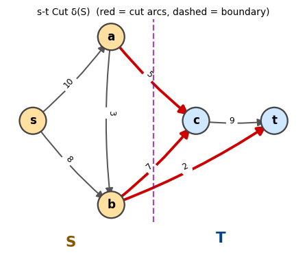 An s,t-cut with \(S\) (yellow) and \(T = N \setminus S\) (blue). Red arcs cross the cut.
Weak duality (flow \(\leq\) cut) is immediate. The deep content is that equality is always achievable.
The lemma is the “weak duality” of flow theory: every feasible flow is bounded above by every feasible cut. The following theorem establishes strong duality — the gap closes at optimality.
- For \(uv \in \delta_D(S)\): \(uv\) is not in \(D'\) so \(x_{uv} = c_{uv}\).
- For \(uv \in \delta_D(\bar{S})\): \(vu\) is not in \(D'\) so \(x_{uv} = 0\).
Therefore flow value \(= x(\delta(S)) - x(\delta(\bar{S})) = c(\delta(S)) - 0 = c(\delta(S))\). By the lemma, this cut is minimum and the flow is maximum. \(\square\)
The proof is remarkable: the reachability set \(S\) simultaneously provides a matching primal (the flow) and dual (the cut) certificate. The flow saturates every forward arc crossing the cut and uses no backward arc — exactly the CS condition for a primal-dual optimal pair.
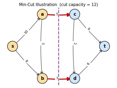 The minimum cut for this network: the red arcs cross from S (yellow) to T (blue), and their capacities sum to the minimum cut capacity.
5.6 Flow Decomposition
Any integral flow can be decomposed into a collection of paths and cycles. This decomposition makes flows “visualizable” and is essential for applying the integrality theorem.
The decomposition proceeds by extracting dipaths one at a time: as long as the flow value is positive, a path must exist (no s,t-cut can be empty), and extracting that path reduces the problem by one. The remaining circulatory flow is then decomposed into cycles by a separate induction. This path-cycle structure is why network flow solutions are easy to interpret physically.
5.7 Combinatorial Applications of Max-Flow Min-Cut
The Max-Flow Min-Cut theorem is a powerful machine for deriving classical combinatorial results. By choosing appropriate network constructions, the theorem instantly yields Menger’s theorems, König’s theorem, and Hall’s theorem — all as special cases of the same LP duality principle.
The arc-disjoint version establishes that the “tightness” in a network (how many independent routes exist between two points) is exactly determined by the minimum bottleneck in arc capacity. The node-disjoint version sharpens this to node capacity — how many independent internal relays the network has. Both are instances of the same underlying max-flow min-cut duality, applied to slightly different network constructions.
Menger’s theorem and König’s theorem are historically prior to the max-flow min-cut theorem — they were proved in the 1920s and 1930s by classical combinatorial arguments. The beauty of the network flow framework is that all three results emerge effortlessly from a single principle: LP strong duality applied to the node-arc incidence matrix. This unification is one of the lasting achievements of combinatorial optimization: deep results that once required separate, clever arguments are now seen as faces of the same mathematical gem.
5.8 Flows with Lower Bounds
Adding lower bounds \(\ell_e > 0\) makes the problem more complex: now each arc must carry at least a minimum amount of flow. This models mandatory usage constraints (e.g., a pipeline that must operate above a minimum throughput to avoid freezing). The key insight is that lower bounds can be “absorbed” into modified supplies and demands at the endpoints.
We can enrich the model with lower bounds \(\ell_e \geq 0\): a feasible flow must satisfy \(\ell_e \leq x_e \leq c_e\). The residual graph for a flow \(x\) has: forward arcs with capacity \(c_e - x_e\), backward arcs with capacity \(x_e - \ell_e\) (preventing flow from dropping below \(\ell_e\)).
5.9 Preflow-Push Algorithm
Ford-Fulkerson and Edmonds-Karp find maximum flows by augmenting along paths from \(s\) to \(t\). The preflow-push algorithm takes a fundamentally different approach: it initially “over-sends” flow from \(s\) (saturating all out-arcs of \(s\)), creating excess at intermediate nodes, and then “pushes” this excess toward \(t\) locally, without worrying about path augmentation. This local approach achieves better worst-case complexity than Edmonds-Karp on dense graphs.
The preflow-push (push-relabel) algorithm achieves better worst-case complexity by working with an infeasible preflow that satisfies the optimality condition throughout, until it becomes a feasible flow.
- \(h(s) = |N|\), \(h(t) = 0\)
- \(h(v) \leq h(u) + 1\) for every arc \(uv\) in the residual graph (no arc points steeply downward)
The height function \(h\) models the “height” at which excess flow “falls” toward the sink. An arc in the residual graph can only carry flow “downhill” (from higher to lower height). The compatibility condition prevents flow from traveling in the wrong direction on residual arcs.
Lemma 6.7.1. If a preflow \(x\) and heights \(h\) are compatible, then the residual graph \(D'\) has no s,t-dipath.
Corollary 6.7.1.1. If a preflow \(x\) is feasible (i.e., has zero excess at all non-source, non-sink nodes) and heights \(h\) are compatible, then \(x\) is a maximum s,t-flow.
This lemma is the key invariant: a compatible preflow is “already optimal” in the sense that no further flow can reach \(t\) from \(s\) in the residual graph. When all excess is cleared, the preflow becomes a maximum flow.
Preflow-Push (Push-Relabel) Algorithm
──────────────────────────────────────
Input:  D=(N,A), capacities c, source s, sink t.
Initialization:
  • h(s) = |N|, h(v) = 0 for all v ≠ s.
  • x_e = c_e for all e ∈ δ_D(s); x_e = 0 otherwise.
Loop:
  While ∃ u ∈ N \ {s,t} with ex(u) > 0:
    If ∃ arc uv ∈ D' with h(v) = h(u) - 1:
      Push: push min{r_uv, ex(u)} along uv.
    Else:
      Relabel: h(u) ← h(u) + 1.
Return x (maximum flow).
Correctness and Complexity:
The analysis of preflow-push is a beautiful piece of amortized bookkeeping. The algorithm performs three types of operations: relabels (height increases), saturating pushes (which remove an arc from the residual graph), and non-saturating pushes (which drain the excess at a node without removing an arc). The key insight is that these three operation types interact in a tightly controlled way: relabels limit how often saturating pushes can repeat on any given arc (since each re-emergence of an arc requires a relabel), and a clever potential function shows that non-saturating pushes are bounded by the sum of potential increases from the other two types of operations. We proceed through the lemmas in sequence, each one tightening the analysis further.
Theorem 6.7.2. The preflow-push algorithm maintains a preflow and a height function compatible with each other throughout its execution.
At termination, no non-source, non-sink node has excess, so the preflow is a feasible flow. By Lemma 6.7.1, the residual graph has no s,t-dipath, so the flow is maximum. Theorem 6.7.2 gives us correctness; now we need termination and a complexity bound. The next lemma is the crucial structural fact: a node with positive excess is always “connected back to the source” in the residual graph, which means the algorithm always has something productive to do and never gets stuck.
Think about why this matters: if a node \(u\) has positive excess but no path back to \(s\) in the residual graph, then the excess is “stranded” — it could never have come from \(s\) in the first place, which would contradict how the preflow was created. The lemma says this cannot happen. As a consequence, the height of any excess node is bounded (Corollary 6.7.3.1), which is what allows us to count relabels.
Termination and Complexity:
Lemma 6.7.3. If \(\mathrm{ex}(u) > 0\), there is a u,s-dipath in \(D'\).
Corollary 6.7.3.1. \(h(u) \leq 2|N| - 1\) throughout the algorithm.
This height ceiling of \(2|N|-1\) is the linchpin of the entire complexity argument. Since each relabel increases a node’s height by at least 1, and each node can be relabeled at most \(2|N|\) times, the total number of relabel operations across the entire algorithm is bounded by \(2|N|^2\). Now we turn to pushes, which we classify into two types because they have very different costs: saturating pushes remove an arc from the residual graph (and are therefore rare in an amortized sense), while non-saturating pushes drain a node’s excess without removing an arc (and must be controlled by a potential function argument).
The dichotomy between saturating and non-saturating pushes is not merely a bookkeeping convenience — it reflects a genuine structural difference. A saturating push is “expensive” in the sense that it changes the residual graph, which then requires relabeling before the same arc can be used again. A non-saturating push leaves the residual graph unchanged, so the same arcs are available for the next step. This is why non-saturating pushes are harder to count: there is no immediate structural consequence that prevents them from happening repeatedly. The potential function argument below handles exactly this challenge.
Definition 6.7.4 (Saturating Push). A push on arc \(uv \in A(D')\) is a saturating push if the full residual capacity \(r_{uv}\) is pushed, i.e., we push \(r_{uv}\) units (arc \(uv\) disappears from \(D'\) after the push).
Definition 6.7.5 (Non-saturating Push). A push on arc \(uv\) is a non-saturating push if we push \(\mathrm{ex}(u) < r_{uv}\) units (node \(u\) loses all its excess but \(uv\) remains in \(D'\)).
Saturating pushes are easy to count because they are self-limiting: after each saturating push on arc \(uv\), that arc disappears from the residual graph and cannot reappear until the flow on \(vu\) is reduced, which requires a push from \(v\) to \(u\), which requires \(v\) to be relabeled. Since relabels are bounded, saturating pushes are bounded.
Theorem 6.7.4. The number of saturating pushes over the entire algorithm is at most \(2|N| \cdot |A|\).
Non-saturating pushes are harder to control because they do not remove any arc — so we cannot use the same counting argument. Instead, we use a potential function \(\Phi\) that tracks the total “height” of all nodes with positive excess. Every non-saturating push decreases \(\Phi\) by at least 1 (the pushing node loses its excess), while relabels and saturating pushes can only increase \(\Phi\) by a controlled amount. Since \(\Phi\) is non-negative, the total decrease from non-saturating pushes is bounded by the total increase from all other operations.
The insight behind choosing \(\Phi = \sum_{v:\,\mathrm{ex}(v)>0} h(v)\) is that it captures how much “work remains”: the higher and more numerous the excess nodes, the more pushing is still needed. A non-saturating push at node \(u\) transfers \(u\)’s entire excess to neighbor \(v\) at height \(h(u)-1\), decreasing \(\Phi\) by \(h(u) - h(v) = 1\). This clean unit decrease per non-saturating push is what makes the accounting precise. The total “budget” of \(\Phi\) increases — from relabels and saturating pushes — is at most \(O(|N|^2 |A|)\), so the number of non-saturating pushes is bounded by the same quantity.
Theorem 6.7.5. The number of non-saturating pushes is at most \(4|N|^2|A|\).
Corollary 6.7.5.1. Preflow-push terminates in \(O(|N|^2|A|)\) operations total.
The chain of lemmas is now complete, and the bound \(O(|N|^2|A|)\) emerges cleanly: relabels contribute \(O(|N|^2)\), saturating pushes contribute \(O(|N||A|)\), and non-saturating pushes — the dominant term — contribute \(O(|N|^2|A|)\). Comparing to Edmonds-Karp’s \(O(|N||A|^2)\), preflow-push is better precisely when the graph is dense (many arcs relative to nodes), while Edmonds-Karp is better for sparse graphs. For the dense networks that arise in practice — complete bipartite graphs for assignment problems, highly connected transportation networks — preflow-push is the algorithm of choice.
It is worth pausing to appreciate the conceptual leap that preflow-push makes relative to earlier algorithms. Ford-Fulkerson and Edmonds-Karp both maintain a globally valid flow at every step: every intermediate state is a legal s,t-flow, just not yet maximum. Preflow-push deliberately breaks this invariant from the start — it over-sends flow out of \(s\), creating excess at interior nodes. This willingness to be “wrong” globally in order to make fast local progress is the hallmark of a new generation of algorithms. The height function provides the global structure that compensates: it guarantees the algorithm is always “going in the right direction,” draining excess toward the sink, even without maintaining a globally valid flow. This idea of maintaining a different invariant — one weaker in some sense but stronger in others — recurs throughout advanced algorithm design, and preflow-push is one of its cleanest illustrations.
5.10 Applications of Maximum Flow
Matrix Rounding. Given a matrix \(M \in \mathbb{R}^{m \times n}\), round each entry to \(\lfloor M_{ij} \rfloor\) or \(\lceil M_{ij} \rceil\) such that every row sum and column sum is also rounded. Model as a flow problem: add source \(s\) and sink \(t\), nodes \(r_i\) (rows) and \(c_j\) (columns). Arc \(s r_i\) has bounds \((\lfloor \text{row}_i \rfloor, \lceil \text{row}_i \rceil)\); arc \(c_j t\) has bounds \((\lfloor \text{col}_j \rfloor, \lceil \text{col}_j \rceil)\); arc \(r_i c_j\) has bounds \((\lfloor M_{ij} \rfloor, \lceil M_{ij} \rceil)\). By integrality, a valid rounding always exists.
Maximum Closure.
The maximum closure problem has a compelling real-world story: the project-selection problem. Imagine a company considering which projects to undertake. Each project \(v\) has a profit (or cost) \(w_v\). But projects have dependencies: if you undertake project \(u\), you must also undertake project \(v\) (represented by arc \(uv\) in a dependency digraph). For example, building a highway (positive profit) might require acquiring right-of-way from multiple landowners (negative cost nodes). You cannot take the highway without taking all the prerequisites. The question is: which subset of projects maximizes total profit, respecting all dependencies?
The mathematical structure of this problem is exactly a closure: a set \(S\) is closed under dependencies if, whenever \(u \in S\) and \(uv \in A\), also \(v \in S\). A closure represents a “self-contained” portfolio of projects. The maximum closure problem asks for the highest-profit such portfolio. What makes this remarkable is that this combinatorial optimization problem — which naively seems to require exhaustive search over exponentially many subsets — reduces to a single max-flow computation.
Definition 6.6.1 (Closure). A closure is a set \(S \subseteq N\) such that \(\delta(S) = \emptyset\) (i.e., \(S\) is closed under outgoing arcs: if \(u \in S\) and \(uv \in A\), then \(v \in S\)).
The reduction to max-flow is ingenious. We add a super-source \(s\) and a super-sink \(t\). Profitable projects (\(w_v > 0\)) get an arc from \(s\) with capacity \(w_v\), representing the profit we “give up” if we don’t select them. Costly projects (\(w_v < 0\)) get an arc to \(t\) with capacity \(-w_v\), representing the cost we incur if we do select them. Dependency arcs get capacity \(\infty\) — the constraint “if you take \(u\), you must take \(v\)” is encoded as an infinite-capacity arc, because cutting it (choosing \(u\) without \(v\)) would be infinitely expensive. A min-cut in this augmented graph corresponds to an optimal closure in the original graph.
Given weights \(w: N \to \mathbb{R}\), find a maximum-weight closure. Add source \(s\) and sink \(t\); for \(w_v > 0\), arc \(sv\) with capacity \(w_v\); for \(w_v < 0\), arc \(vt\) with capacity \(-w_v\); original arcs with capacity \(\infty\).
Proposition 6.6.1. An s,t-cut \(\delta(S)\) in the new digraph has finite capacity if and only if \(S \setminus \{s\}\) is a closure in the original digraph.
Proposition 6.6.2. The weight of the closure \(S \setminus \{s\}\) equals \(c(\delta(s)) - c(\delta(S))\).
Proposition 6.6.3. Since \(c(\delta(s)) = \sum_{w_v > 0} w_v\) is fixed, maximizing the weight of the closure is equivalent to minimizing \(c(\delta(S))\), which is solved by a maximum flow / minimum cut computation.
Max closure weight \(= \sum_{w_v > 0} w_v - \min\text{-cut}\).
Notice the elegance of the reduction: the three propositions (6.6.1, 6.6.2, 6.6.3) together give a complete recipe: build the auxiliary network, run max-flow to find a min-cut, and read off the optimal project selection from which side of the cut each node falls on. The formula \(\text{max weight} = \sum_{w_v > 0} w_v - \min\text{-cut}\) makes intuitive sense: start by assuming you take all profitable projects, then subtract the minimum-cost “damages” — the cut capacity — needed to fix all violated dependencies. The max-flow algorithm finds the most efficient way to repair violations, and what remains is the optimal portfolio weight.
Chapter 6: Global Minimum Cuts
The max-flow min-cut theorem answers the question: “What is the minimum cut capacity separating a specific pair \((s,t)\)?” But many applications require the global minimum cut: the partition of the entire node set that is hardest to sever, without specifying which side is source and which is sink. In network reliability engineering, the global min-cut measures how many wires must fail before the network disconnects. In VLSI design, it measures the minimum chip area where a circuit can be partitioned. In community detection, it identifies the weakest seam between clusters in a graph. These applications need a minimum over all possible cuts, not just \(s,t\)-cuts for a fixed pair.
6.1 Global Minimum Cut in Directed Graphs (Hao-Orlin)
A global minimum cut of a digraph \(D\) is a non-trivial set \(S \subsetneq N\) minimizing \(c(\delta(S))\).
The naive brute-force approach is to try all \(O(|N|^2)\) source-sink pairs, computing a max-flow for each. This works but is expensive: \(O(|N|^2)\) max-flow computations gives an overall complexity of \(O(|N|^2)\) times the per-flow cost. A simple observation cuts this in half: fix any node \(s\); the global minimum cut either has \(s\) on one side or the other, so we only need to compute minimum \(s,t\)-cuts for all other \(t \in N\) (and also minimum \(t,s\)-cuts for all \(t\), since the digraph is directed). That is \(2(|N|-1)\) max-flows — better, but still \(O(|N|)\) max-flow computations. The Hao-Orlin algorithm achieves something remarkable: it finds the global minimum s-cut in the same asymptotic time as a single max-flow, by running all \(|N|-1\) required max-flow computations simultaneously using a modified preflow-push.
Naive approach: Run max-flow for all \(O(|N|^2)\) source-sink pairs. A simple improvement: fix any \(s \in N\); \(s\) is on one side of the global min cut. Find the minimum s,t-cut for all \(t \in N\) (and reverse-direction cuts). This requires \(2(|N|-1)\) max-flow computations.
Hao-Orlin does better by solving all minimum s-cuts simultaneously using a modified preflow-push.
Generic Algorithm for Minimum s-Cut
──────────────────────────────────────
1. Set X = {s}.
2. While X ≠ N:
   a. Pick t ∉ X; find a minimum X,t-cut δ(S*).
   b. Store δ(S*). Add t to X.
3. Output the minimum over all stored cuts.
Correctness: Let \(\delta(S^*)\) be a global minimum s-cut. Consider the first time \(t \notin S^*\) is chosen. At that moment, \(X \subseteq S^*\), so \(\delta(S^*)\) is an X,t-cut. The algorithm finds a minimum X,t-cut \(\delta(\hat{S})\) with \(c(\delta(\hat{S})) \leq c(\delta(S^*))\). But \(\delta(\hat{S})\) is also an s-cut, so \(c(\delta(\hat{S})) \geq c(\delta(S^*))\). Hence both cuts have the same capacity.
Hao-Orlin implements the Generic Algorithm by modifying the preflow-push to maintain an X-preflow and track cut levels.
- \(h(v) = |N|\) for all \(v \in X\)
- \(h(t) \leq |X| - 1\)
- \(h(v) \leq h(u) + 1\) for all \(uv \in A(D')\)
Lemma 7.2.1. If \(\ell\) is a cut-level and \(\mathrm{ex}(v) = 0\) for all \(v\) with \(h(v) < \ell\) (except \(t\)), then \(\{v : h(v) \geq \ell\}\) is a minimum X,t-cut.
Hao-Orlin Algorithm
──────────────────────
Initialization:
  X = {s}; pick t ∉ X; h(s) = |N|, h(v) = 0 otherwise;
  ℓ = |N| - 1; push as much flow out of X as possible.
While X ≠ N:
  Run push-relabel with exceptions:
    (a) Only select v with ex(v) > 0 and h(v) < ℓ.
    (b) If we would relabel v and v is the only node at height h(v):
        instead set ℓ = h(v).   (maintain non-empty levels consecutive)
    (c) If we would relabel v to ℓ: relabel but reset ℓ = |N| - 1.
  When no node has ex(v) > 0 and h(v) < ℓ:
    Store cut {v : h(v) ≥ ℓ} (this is a minimum X,t-cut by the Lemma).
    Add t to X; set h(t) = |N|; push all flow out of t.
    Pick new t = node with lowest height; reset ℓ = |N| - 1.
Output minimum over all stored cuts.
Key invariants maintained by Hao-Orlin (proved below):
The five lemmas that follow may seem technical in isolation, but they serve a unified purpose: they collectively certify that Hao-Orlin’s modified preflow-push never “breaks” the height structure that makes preflow-push correct. Lemma 7.2.2 controls the level structure (no gaps); Lemma 7.2.3 controls the current target node’s height (bounded by \(|X|\)); Lemma 7.2.4 uses 7.2.3 to bound all non-\(X\) heights; and Lemma 7.2.5 uses 7.2.4 to guarantee that the threshold \(\ell = |N|-1\) is always a cut level. Think of the lemmas as a chain of checks, each one building on the previous to maintain the invariant that the algorithm is always in a valid state to read off a minimum cut.
Lemma 7.2.2. Throughout Hao-Orlin, the non-empty levels below \(|N|\) are consecutive.
Consecutive levels are essential for the cut-level detection mechanism: a cut level is a “gap” in the height structure — no arc crosses from level \(k\) to level \(k-1\) — and the algorithm uses these gaps to identify minimum cuts. By preserving consecutive levels, Hao-Orlin ensures that whenever it detects a gap (and sets \(\ell\)), the gap is genuine and the corresponding set \(\{v : h(v) \geq \ell\}\) is indeed a valid minimum X,t-cut. Without Lemma 7.2.2, a gap might be an artifact of an empty level rather than a true structural barrier.
Lemma 7.2.3. \(h(t) \leq |X| - 1\) throughout the algorithm.
Lemma 7.2.3 is an elegant “co-evolution” invariant: as \(X\) grows by absorbing one node per outer iteration, the height of the new target node \(t\) is allowed to grow by at most 1. The two quantities \(h(t)\) and \(|X|\) march upward together, maintaining the inequality throughout. This is the compatibility condition (2) for X-preflows, so Lemma 7.2.3 is precisely what we need to invoke the definition of a compatible X-preflow.
Corollary 7.2.3.1. The algorithm maintains compatible X-preflow and heights throughout.
With compatibility guaranteed, we can use Lemma 7.2.1 in each inner iteration: whenever the inner loop terminates (no more excess below level \(\ell\)), the level set \(\{v : h(v) \geq \ell\}\) is a minimum X,t-cut. The remaining lemmas close in on the height bounds needed to ensure the overall run time matches that of a single preflow-push.
Lemma 7.2.4. \(h(v) \leq |N| - 2\) for all \(v \notin X\) throughout the algorithm.
The bound \(h(v) \leq |N|-2\) for non-\(X\) nodes is exactly what is needed to show that level \(|N|-1\) is always empty (when \(\ell = |N|-1\)), and hence always a cut level. This completes the invariant chain.
Lemma 7.2.5. \(\ell\) is always a cut level when \(\ell = |N| - 1\).
Corollary 7.2.5.1. \(\ell\) is always a cut level throughout the algorithm.
The five lemmas (7.2.1–7.2.5) above, together with Corollaries 7.2.3.1 and 7.2.5.1, collectively establish that Hao-Orlin’s modified preflow-push correctly maintains compatible X-preflows throughout, always produces a valid minimum X,t-cut when the inner loop terminates, and does so without exceeding the height bounds established for standard preflow-push. The consequence is Theorem 8.1.1 — that the entire global min-cut computation, solving all \(|N|-1\) successive subproblems, costs no more than a single run of preflow-push.
Theorem 8.1.1 (Hao-Orlin). The global minimum s-cut can be found in \(O(|N|^2|A|)\) time — the same asymptotic complexity as a single preflow-push computation.
Why does running \(|N|-1\) successive max-flow problems cost the same as running one? The key is that Hao-Orlin reuses the preflow structure: when \(t\) is absorbed into \(X\), the current preflow and heights are not discarded but updated incrementally. The total number of relabels, saturating pushes, and non-saturating pushes accumulated across all \(|N|-1\) phases is bounded by the same \(O(|N|^2|A|)\) that bounds a single preflow-push. This amortized efficiency — doing more work for the same asymptotic cost — is a recurring theme in advanced algorithm design, and Hao-Orlin is one of its most elegant instances.
The contrast between Hao-Orlin and the naive approach is instructive. Naively, \(|N|-1\) max-flow computations each costing \(O(|N|^2|A|)\) would give \(O(|N|^3|A|)\) total. Hao-Orlin achieves \(O(|N|^2|A|)\) — a factor of \(|N|\) better — by never throwing away progress. Each time a target node \(t\) is absorbed into \(X\), the existing preflow and height structure already encode information about the capacities toward \(t\). Updating rather than restarting is the algorithmic dividend that makes Hao-Orlin powerful. This insight — that carefully maintained intermediate state can be reused across multiple subproblems — is one of the deepest ideas in combinatorial optimization, and it appears again in the next section in a very different guise: randomized contraction.
6.2 Global Minimum Cut in Undirected Graphs (Karger’s Algorithm)
For undirected graphs \(G = (V, E)\) with edge capacities \(c \in \mathbb{R}^E_+\), we want the minimum capacity non-trivial cut.
Karger’s Algorithm repeatedly contracts a random edge (with probability proportional to its capacity) until only 2 supernodes remain. The remaining edges form a cut.
Karger's Algorithm
──────────────────────
Input:  Undirected graph G=(V,E) with capacities c.
1. While |V| > 2:
   a. Select edge uv with probability c_{uv} / Σ_{e ∈ E} c_e.
   b. Contract uv: merge u,v; keep parallel edges; remove self-loops.
2. Output the cut defined by the two remaining supernodes.
Corollary 8.1.1.1. Running Karger’s algorithm \(\alpha |V|^2\) times and outputting the minimum cut found gives a minimum cut with probability at least \(1 - e^{-2\alpha}\).
The total cost of running \(\alpha|V|^2\) repetitions is \(O(|V|^4 \log |V|)\) — elegant and easily parallelized.
Karger’s algorithm is a beautiful example of randomized algorithm design. Unlike Hao-Orlin, which relies on carefully maintained preflow-push invariants, Karger uses probabilistic analysis: the probability that the minimum cut survives a single run is at least \(\binom{|V|}{2}^{-1}\), which is small but non-trivial. By repeating the algorithm \(O(|V|^2)\) times and taking the best result, we achieve high success probability via the union bound. The key observation is that there can be at most \(\binom{|V|}{2}\) distinct global minimum cuts (since each one survives with the above probability, and the probabilities can sum to at most 1), which is a striking combinatorial fact in its own right. Karger’s algorithm also illustrates a recurring principle: for some problems, the best approach is not to maintain complex invariants but to use randomness to search the solution space efficiently. The comparison of Hao-Orlin and Karger — one deterministic and algebraically intricate, the other randomized and combinatorially simple — shows that there is rarely a single “correct” approach to a problem; the right algorithm depends on the structure of the specific problem and the constraints of the application.
Summary of Key Theorems and Running Times
| Algorithm | Problem | Running Time | Notes |
|---|---|---|---|
| Network Simplex | TP / MCFP | Not polynomial in general | Exponential worst-case; excellent in practice |
| Ford’s Algorithm | Shortest paths | Pseudopolynomial / may not terminate | General negative costs; does not terminate on neg. di-cycles |
| Bellman-Ford | Shortest paths | \(O(\|N\| \cdot \|A\|)\) | Detects negative di-cycles |
| Dijkstra | Shortest paths (non-neg.) | \(O(\|N\| \log \|N\| + \|A\|)\) | Requires \(w \geq 0\); Fibonacci heap |
| Ford-Fulkerson | Max flow | Pseudopolynomial | Integer caps only; may not terminate for irrationals |
| Edmonds-Karp | Max flow | \(O(\|N\| \cdot \|A\|^2)\) | Polynomial; BFS shortest augmenting path |
| Preflow-Push | Max flow | \(O(\|N\|^2 \|A\|)\) | Better for dense graphs |
| Hao-Orlin | Global min cut (directed) | \(O(\|N\|^2 \|A\|)\) | Modification of preflow-push; finds all s-cuts |
| Karger | Global min cut (undirected) | \(O(\|V\|^4 \log \|V\|)\) (randomized) | Probability \(\geq 1 - e^{-2\alpha}\) after (\alpha |
The duality perspective unifies everything: in every problem, the optimality conditions are complementary slackness conditions on a primal-dual LP pair. Understanding duality is understanding why these algorithms work and when they stop.