CO 342: Introduction to Graph Theory

These notes are based on Felix Zhou’s course notes. Additional explanations, visualizations, and examples have been added for clarity.

Graph theory is one of the most beautiful branches of combinatorics. Its objects — vertices, edges, paths, and cycles — are simple enough to draw on a napkin, yet they give rise to deep theorems whose proofs require genuine ingenuity. This course, CO 342 at the University of Waterloo (Fall 2019), covers the classical core of the subject: trees, coloring, matchings, connectivity, planar graphs, and the interplay between them.

Chapter 1: Review

This chapter revisits foundational material from prerequisites (Math 249 / CO 250 level), establishing notation and the key theorems we will use throughout. Even familiar results are stated precisely, because graph theory rewards careful definitions.

Trees and Forests

Before we can analyze more intricate graph properties, we need to understand the simplest connected structures. Trees are graphs with exactly enough edges to stay connected — remove any one edge and they fall apart; add any one edge and they gain a cycle. This minimality is what makes them so fundamental.

A tree is a connected acyclic graph. A forest is an acyclic graph (equivalently, a disjoint union of trees). These are among the most fundamental objects in combinatorics: they appear in algorithm design, network routing, phylogenetics, and data structures.

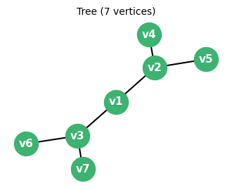
A balanced binary tree with 7 vertices — a prototypical tree structure.

One elementary but important fact about forests is that they always have “leaf” vertices — degree-1 vertices that can be removed without disconnecting anything. The proof is elegant: just follow the longest path.

One elementary but important fact about forests is that they always have “leaf” vertices — degree-1 vertices that can be removed without disconnecting anything. The proof is elegant: just follow the longest path.

The proof strategy here is extremal: pick the longest possible path, then argue that its endpoint must be a leaf. This “longest path” trick recurs throughout graph theory. The existence of leaves is what makes induction on trees so natural — one peels off leaves one at a time.

A useful equivalent characterisation: a graph on \(n\) vertices is a tree if and only if it is connected and has exactly \(n-1\) edges. Trees have exactly one face when drawn as plane graphs, reflecting the formula \(v - e + f = 2\) applied to forests.

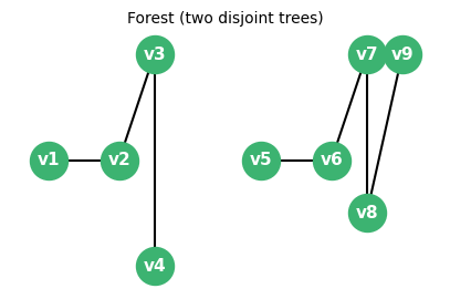
A forest consisting of two disconnected trees — the union of trees with no extra edges.

Graph Colorings

Coloring problems are among the oldest questions in graph theory, tracing back to the four-color problem for maps posed in 1852. The central question is: how few colors suffice to color the vertices of a graph so that no two adjacent vertices share a color? This models scheduling conflicts, register allocation in compilers, and frequency assignment in wireless networks.

A proper \(k\)-coloring of a graph \(G\) assigns one of \(k\) colors to each vertex such that adjacent vertices receive different colors. The chromatic number \(\chi(G)\) is the minimum \(k\) for which a proper \(k\)-coloring exists.

The chromatic number captures a fundamental tension: dense local structure (large cliques, odd cycles) forces many colors, while sparse or bipartite structure allows few. It is generally NP-hard to compute, but upper bounds from simple greedy algorithms are both easy to prove and quite useful.

The simplest upper bound on \(\chi(G)\) comes from a greedy argument: color vertices one at a time, assigning each vertex the smallest color not used by its already-colored neighbors.

The proof uses a “greedy extension” strategy: the inductive hypothesis provides a coloring of a smaller graph, and we verify that the removed vertex can always be reintegrated. This technique — remove one element, induct, reattach — is ubiquitous in graph theory.

The bound \(\Delta + 1\) is tight for complete graphs \(K_n\) (where \(\Delta = n-1\) and \(\chi = n\)) and for odd cycles \(C_{2k+1}\) (where \(\Delta = 2\) and \(\chi = 3\)). Brooks’ theorem (beyond the scope of this course) strengthens the bound: if \(G\) is connected, not a complete graph, and not an odd cycle, then \(\chi(G) \leq \Delta\).

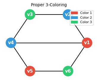
A proper 3-coloring: no two adjacent vertices share a color.

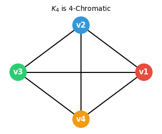
The complete graph \(K_4\) requires exactly 4 colors — it is 4-chromatic.

The celebrated Four Color Theorem (Appel-Haken, 1976) states that every planar graph is 4-colorable. This is one of the deepest results in combinatorics and was the first major theorem proved with computer assistance.

Matchings

Matchings are a central topic in combinatorial optimization. A matching captures the idea of pairing up elements of a set subject to compatibility constraints — scheduling workers to shifts, assigning residents to hospitals, or routing packets in a network. The goal is typically to find the largest or most efficient such pairing.

A matching is a collection of vertex-disjoint edges; each vertex can be “used” at most once. This models one-to-one assignments: each worker gets at most one shift, each resident gets at most one hospital.

Whether a vertex is “covered” by a matching is crucial for characterizing optimal matchings; exposed vertices are precisely those that an augmentation can eliminate.

A perfect matching is the most desirable outcome: everyone gets paired. The parity restriction is a simple but fundamental obstruction — odd-order graphs can never be perfectly matched.

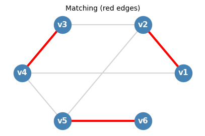
Red edges form a matching: each vertex is incident to at most one red edge.

The distinction between maximal and maximum matchings deserves emphasis. A matching is maximal if no edge can be added to it; it is maximum if no matching has more edges. Every maximum matching is maximal, but the converse fails.

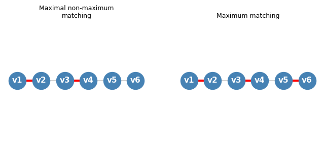
Left: a maximal matching of size 2 (cannot extend, but not maximum). Right: a maximum matching of size 3 on the same path graph \(P_6\).

1.3.1 Hall’s Theorem

With the definitions in place, the central question is: when does a bipartite graph have a matching that covers one entire side? Clearly a necessary condition is that every group of vertices on the left side must collectively have “enough” neighbors on the right. Remarkably, this necessary condition is also sufficient.

The most important theorem in matching theory is Hall’s Marriage Theorem (1935), which gives a complete combinatorial characterization of when a bipartite graph has a matching saturating one side. Its name comes from the following metaphor: we have a set \(X\) of men and a set \(Y\) of women, with edges indicating compatibility. When can every man be matched to a compatible woman?

To state Hall’s theorem, we need the notion of neighborhood — the “reach” of a set of vertices.

The neighborhood measures how many “slots” on the right side are accessible from a set \(S\) on the left. If \(|\Gamma(S)| < |S|\) for some \(S\), then \(S\) has too few neighbors to be matched — a combinatorial obstruction.

Hall’s Condition is a necessary condition for a matching saturating \(X\): if any \(k\) vertices on the left have fewer than \(k\) neighbors on the right, they cannot all be matched. Remarkably, it is also sufficient.

The following key theorem establishes that Hall’s Condition is not merely necessary but sufficient — a local neighborhood condition completely controls a global matching property.

The proof strategy is inductive, splitting into cases based on whether a “tight” set (one where equality \(|\Gamma(S_0)| = |S_0|\) holds) exists. Tight sets are natural bottlenecks: they must be matched entirely within their neighborhood, and this constraint propagates through the induction cleanly.

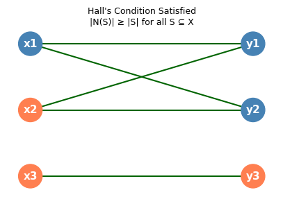
Hall’s Condition satisfied: every subset \(S \subseteq X\) has \(|\Gamma(S)| \geq |S|\). A perfect matching exists.

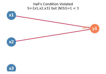
Hall’s Condition violated: \(S = \{x_1,x_2,x_3\}\) but \(|N(S)| = 1 < 3\). No matching saturating \(X\) exists.

Hall’s theorem immediately yields a satisfying consequence for symmetric, regular graphs.

The proof uses a double-counting argument on edges — a technique that will recur in Euler’s formula and König’s theorem. Regularity enforces uniform Hall’s Condition almost for free.

1.3.2 Berge’s Theorem

Hall’s theorem tells us when a perfect matching exists. Berge’s theorem tells us when a matching is as large as possible — and provides an algorithmic way to check. The key concept is an augmenting path: a path that starts and ends at unmatched vertices, which we can “flip” to gain one more matching edge.

Berge’s theorem characterizes maximum matchings via augmenting paths — alternating paths that start and end at exposed vertices, and can be used to increase the matching size.

Alternating paths weave in and out of the current matching; they are the “modification paths” along which we can locally restructure the matching.

An augmenting path begins and ends outside the matching, so swapping matched and unmatched edges along it strictly increases the matching size by one. The existence of such paths is exactly the obstruction to optimality.

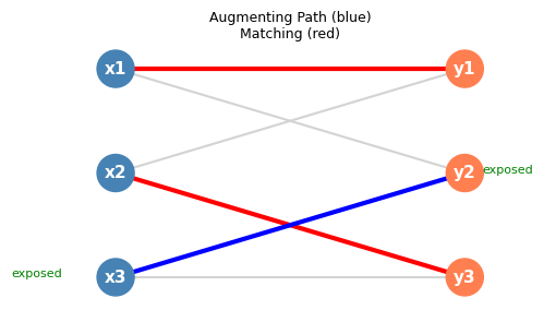
Current matching in red; augmenting path in blue connecting two exposed vertices. Swapping along the blue path increases the matching by one.

Animated: the augmenting path algorithm on a bipartite graph, step by step.

Berge’s 1957 theorem establishes the elegant equivalence between the absence of augmenting paths and the optimality of the matching.

This theorem provides the conceptual basis for all matching algorithms: to find a maximum matching, repeatedly search for augmenting paths and augment until none remain. It also shifts the computational question from “is this matching maximum?” to “does an augmenting path exist?” — the latter being answerable by graph search.

Vertex Covers

Having understood matchings — sets of edges with no shared vertices — we now turn to their natural “dual” structure. A vertex cover is a set of vertices that “hits” every edge. The interplay between the two is one of the most beautiful min-max dualities in combinatorics.

Intuitively, a vertex cover “guards” every edge by selecting a sentinel at one endpoint. Every complement of an independent set is a vertex cover — the two concepts are dual to each other.

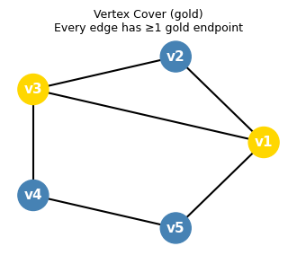
Gold vertices form a vertex cover: every edge touches at least one gold vertex.

Matchings and vertex covers are dual to each other in the following fundamental sense: a large matching forces a large cover, and the two sizes are always within a factor of two. The following inequality is immediate:

The factor-of-two gap between \(\nu\) and \(\tau\) is tight for general graphs (achieved by \(K_3\)), but for bipartite graphs it collapses to perfect equality. This is König’s theorem.

König’s Theorem

For bipartite graphs, the inequality \(\nu \leq \tau\) becomes an equality — a remarkable fact with no analogue for general graphs.

König’s theorem is the cornerstone of bipartite matching theory, establishing a perfect min-max duality between matchings and covers that will be echoed throughout the course.

The proof is a beautiful example of using one theorem (Hall’s) to prove another: the minimum cover structure forces Hall’s Condition on the two sides of the bipartition, which supplies the matchings that witness the lower bound on \(\nu\).

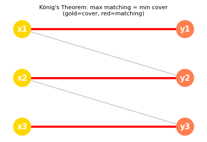
Gold nodes form a minimum vertex cover; red edges form a maximum matching. König’s theorem guarantees their sizes are equal in bipartite graphs.

König’s theorem fails for non-bipartite graphs: the triangle \(K_3\) has \(\nu = 1\) but \(\tau = 2\). The obstruction is odd cycles, which cannot be perfectly matched.

Chapter 2: Introduction

Chapter 1 used informal graph-theoretic language, relying on intuition. Chapter 2 lays the rigorous foundations — the axiomatic definition of a graph — that make it possible to state theorems precisely and handle degenerate cases (loops, parallel edges, disconnected graphs) without ambiguity. This precision pays dividends immediately in the theory of planar graphs and their duals.

Formal Definitions

Graph theory requires a careful general definition of “graph” that handles loops and parallel edges. Felix Zhou’s notes follow the Diestel convention:

This formal triple-based definition is more general than the familiar “set of vertices and set of edges” description from undergraduate courses. The advantage appears in dual graph constructions: if \(G = (V, E, i)\) is a plane graph with faces \(F\), its dual \(G^* = (F, E, j)\) uses the same edge set \(E\) with a new incidence function \(j\), naturally handled by this framework.

The dual construction exemplifies why the triple \((V, E, i)\) formulation is preferable to the pair \((V, E)\): the same edge set plays different roles in \(G\) and \(G^*\).

Adjacency and incidence are the elementary relationships between vertices and edges; all higher graph structure is built from them.

The degree measures how many edge-ends attach to a vertex — the fundamental quantity in handshaking arguments and in characterizing regular graphs.

The Handshaking Lemma states that \(\sum_{v \in V} \deg(v) = 2|E|\), since each edge contributes exactly 2 to the total degree sum.

These basic notions — walks, paths, circuits — are the building blocks for all connectivity arguments. Paths are the most restrictive: no repeated vertices. Circuits are the minimal “loops” in a graph; their absence defines forests and trees.

Components partition the vertex set into maximal connected pieces; the entire theory of graph decomposition rests on this elementary observation.

To study local structure, we need the notion of a subgraph — a graph contained within another.

Induced subgraphs are the “natural” restriction to a vertex subset — they inherit all relationships between chosen vertices. They arise constantly when studying connectivity: removing a vertex \(v\) yields the induced subgraph \(G[V \setminus \{v\}]\).

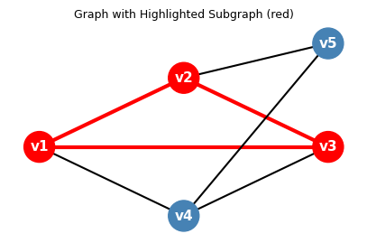
Red vertices and edges form an induced subgraph: all edges between red vertices are included.

Graph Families and Basic Notions

With the formal definition in place, we can catalogue the most important named graph families. These serve as both examples and extremal cases throughout the course.

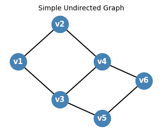
A simple undirected graph on 6 labeled vertices: the fundamental combinatorial object.

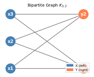
The complete bipartite graph \(K_{3,2}\): every vertex on the left is adjacent to every vertex on the right.

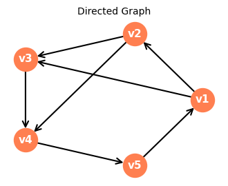
A directed graph (digraph): edges have orientation, represented by arrows.

Connectivity is the most basic structural property of a graph: does it hang together as a single piece, or does it split into isolated islands? (See Definition 2.1.7 above for the formal statement.)

Components partition the vertex set into maximal connected pieces. Much of graph theory — Euler’s formula, Menger’s theorem, the block-cut tree — is stated for connected graphs, and the general case reduces to component-by-component analysis.

A key fact: a bipartite graph is characterized by having no odd cycles. The BFS 2-coloring check assigns alternating colors during a breadth-first traversal; a contradiction (adjacent vertices of the same color) occurs precisely when an odd cycle is found.

BFS coloring animation: vertices are colored alternately as the BFS frontier expands. If a conflict arises, the graph is not bipartite.

Chapter 3: Connectedness

Moving from local structure to global robustness: Chapter 3 asks not merely whether a graph is connected, but how strongly it is connected. Connectivity measures how “robustly” a graph is connected: how many vertices or edges must be removed to disconnect it. This is crucial in network reliability, VLSI design, and algorithm complexity. The chapter culminates in Menger’s theorem, a min-max result that will reappear in a different guise as the max-flow min-cut theorem in network flows.

Connectivity and Cut Vertices

Before defining connectivity, we set up the foundational vocabulary of paths, separators, and graph operations.

The component decomposition is the coarsest structural fact about a graph: it partitions vertices into maximal islands that have no edges between them. Once we understand components, connectivity theory asks a sharper question — not just whether two vertices are connected, but how robustly so.

Graph union formalizes what it means to “paste” two graphs together at shared structure. The direct sum is the cleaner notion: the two graphs share nothing, so there is no ambiguity about edges between them. This becomes essential when we state that a graph is the disjoint union of its components.

The direct sum is simply the disjoint union — the formal counterpart of the intuitive picture of a graph falling into separate pieces. This unique decomposition means we can almost always reduce proofs about general graphs to proofs about connected graphs, handling each component independently.

Subtraction is the key operation for studying robustness: deleting a set \(X\) of vertices or edges and asking whether the remainder is still connected is exactly how we measure connectivity. Notice that deleting a vertex automatically removes all its incident edges — we do not leave “dangling” edge-ends behind.

The \(AB\)-path formulation is crucial for Menger’s theorem: it captures the idea of a path “traveling from one side to the other” without touching either side internally, exactly what is needed for the combinatorial counting argument to work.

A separator consisting of a single edge — a bridge — represents the most extreme form of fragility: one edge stands between connectivity and disconnection. Think of a bridge as a literal bridge over a river: if it collapses, the two banks have no way to communicate. The definition parallels the cut vertex definition above, simply replacing the vertex by an edge in the separator.

Bridges are the most fragile edges in a graph: they single-handedly hold together two otherwise disconnected regions. Networks relying on bridge edges are highly vulnerable — losing that one edge disrupts all communication. The block-cut tree, defined shortly, organizes the bridge structure into a clean hierarchy.

To quantify robustness, we define \(k\)-connectivity: a graph is \(k\)-connected if no set of fewer than \(k\) vertices can disconnect it.

Higher connectivity means greater fault tolerance: a 3-connected network remains functional after any two nodes fail. The connectivity \(\kappa(G)\) is a single number that summarizes this structural robustness.

Cut vertices are the individual points of failure — vertices whose removal breaks the graph apart. They are the local manifestation of low connectivity.

Key equivalences: being 1-connected is the same as being connected (and not a singleton). Being 2-connected means connected with no cut vertex (with the exception of the single-edge graph \(K_2\)). Cut vertices are precisely the bottlenecks through which all traffic between certain parts of the graph must pass.

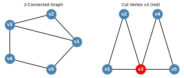
Left: a 2-connected graph (no cut vertex). Right: vertex \(v_3\) in red is a cut vertex — removing it disconnects the graph into two triangles.

Rather than characterizing 2-connectivity by what is absent (cut vertices), the following theorem characterizes it constructively — showing how 2-connected graphs can be built up step by step.

Think of an ear as a “bridge addition”: rather than attaching a single edge, we attach a whole path whose two endpoints already exist in the graph but whose interior is entirely new. Each ear adds new internal vertices and creates new cycles, incrementally increasing the connectivity and the number of independent paths.

This constructive characterization is very useful: it shows that 2-connected graphs have a “layered” structure that can be built incrementally. Ear decompositions are also the basis for efficient algorithms that find 2-connected components in linear time.

The Block Graph

With cut vertices identified, we can decompose any graph into its irreducible 2-connected pieces. These pieces — the blocks — are joined together at cut vertices, and the global structure is captured by a tree.

Blocks are the “atoms” of connectivity: within a block, there are no bottleneck vertices. Bridges — single edges that are blocks — are the most vulnerable connections in the graph.

The block-cut tree is a beautiful structural decomposition: it reveals exactly how the 2-connected pieces are joined together at cut vertices, like beads on a string. That the block-cut tree is always a tree (never has cycles) reflects the fact that blocks can only share vertices at cut vertices — never at interior vertices — so the graph of their “interactions” is acyclic.

The key structural fact is that blocks partition the edges, and overlap only at cut vertices.

The proof argument is a “union of 2-connected graphs sharing two vertices is 2-connected” fact. This tells us blocks genuinely partition the edge set: every edge belongs to exactly one block.

Strong Orientation

The block-cut tree and ear decompositions characterize the undirected structure of a 2-connected graph. Here we add a direction to each edge — asking: when can we orient every edge of \(G\) so that the resulting directed graph is strongly connected, meaning there is a directed path from any vertex to any other vertex? This question arises naturally in traffic engineering (one-way roads), network routing, and tournament scheduling.

An orientation of a graph \(G\) is an assignment of a direction to each edge: each edge \(\{u,v\}\) becomes either the arc \(u \to v\) or \(v \to u\). A directed \(u\)-\(v\) path is a sequence \(u = v_0, v_1, \ldots, v_k = v\) where each consecutive pair forms a directed arc \(v_i \to v_{i+1}\). A strong orientation is one in which there exists a directed \(u\)-\(v\) path for every ordered pair of vertices \((u, v)\). In a strongly oriented graph, you can navigate from any location to any other location — even though every road is one-way.

The fundamental obstacle to a strong orientation is immediately apparent: if \(G\) has a cut edge (bridge), then any orientation of that edge makes traversal in one direction impossible. Removing a bridge disconnects the graph, so the two components cannot communicate after one direction is chosen. This suggests that the right condition is 2-edge-connectivity.

The forward direction is the observation above: a bridge forces a bottleneck that cannot be navigated in both directions. The reverse direction says that the absence of bridges is sufficient — a remarkable fact that says 2-edge-connectivity is already enough. The proof of sufficiency uses the block structure and the ear decomposition to construct the orientation inductively.

We first establish the key building block: 2-connected graphs are strongly orientable.

Notice the proof is constructive: the ear decomposition algorithm simultaneously finds the decomposition and builds the strong orientation. The orientation direction of each ear is arbitrary; flipping it would give a different but equally valid strong orientation.

Now we extend to the general case using the block-cut tree. The key observation is that blocks are the “atoms” of orientation — a strong orientation of the whole graph is equivalent to a strong orientation of each block independently.

Combining both theorems yields Robbins’ theorem: since a block is either an isolated vertex (no orientation needed), a bridge (which has no strong orientation), or a 2-connected graph (which does have a strong orientation), a connected graph is strongly orientable if and only if none of its blocks are bridges — which is precisely the condition of 2-edge-connectivity.

This characterization is clean and satisfying. The proof of the ear decomposition theorem (that 2-connected graphs have ear decompositions) is the hidden engine: it converts the global property of 2-connectivity into a constructive inductive structure that can carry the orientation forward. The ear decomposition is the right notion of “how 2-connected graphs are built,” and this theorem is one of its first payoffs.

Contractions and Tutte’s Theorem

Edge contraction is the operation of “collapsing” an edge into a single vertex, merging the two endpoints. This simple operation is the key to inductive proofs about 3-connected graphs and to the theory of graph minors, which culminates in one of the deepest theorems in mathematics (Robertson-Seymour, 2004).

Contraction is the dual of subdivision. Together with deletion, it generates the minor relation, which underlies some of the deepest theorems in graph theory (Robertson-Seymour). After contracting \(e\), the new vertex \(x_{uv}\) represents the “merged” pair \(\{u,v\}\); the neighbors of \(x_{uv}\) are exactly all former neighbors of either endpoint.

This lemma says that a minimum separator does not “waste” any of its vertices — every member of a minimum cut genuinely participates in blocking some connection. It is used in Tutte’s proof to derive a contradiction: if every edge of a 3-connected graph created a problem when contracted, one could extract an impossibly small separator.

Notice that this commutativity requires the sets acted on to be disjoint: the deletion set \(X\) must not touch the contracted edge or its endpoints. When this disjointness holds, the two operations commute — we can delete first and contract second, or vice versa, with identical results.

This commutativity of deletion and contraction is used repeatedly in inductive arguments — it allows us to freely switch the order of these operations when they act on disjoint parts of the graph.

The following result shows that 2-connectivity is “stable” under edge operations: we can always contract or delete without completely destroying connectivity.

This proposition enables inductive proofs on 2-connected graphs: either \(G/e\) or \(G - e\) is a smaller 2-connected graph to which we may apply the inductive hypothesis. The case \(|V(G)| > 3\) is necessary: the triangle \(K_3\) is 2-connected, but deleting any edge gives a path (not 2-connected) and contracting any edge gives \(K_2\) (not 2-connected either). Beyond four vertices, however, at least one operation always preserves 2-connectivity, giving the inductive step we need.

A basic degree condition on connectivity: high connectivity forces high minimum degree, since a vertex of low degree can be disconnected by deleting its small neighborhood.

This provides a simple necessary condition that rules out many graphs from being highly connected at a glance.

The \(K_{3,3}\) example highlights an important subtlety: deletion can immediately violate 3-connectivity even when the original graph is highly structured. It also shows that for cubic (3-regular) graphs, the only available operation to preserve 3-connectivity is contraction — deletion always creates degree-2 vertices. This makes Tutte’s theorem — which guarantees a contractible edge in every 3-connected graph — especially powerful for the cubic setting.

The 8-wheel example is instructive precisely because it shows that not every edge of a 3-connected graph can be contracted — some edges are “essential” in both directions. The power of Tutte’s theorem is that it guarantees at least one contractible edge always exists, even if most edges are essential.

Wheels are the extremal examples showing Tutte’s Wheel Theorem is tight: every edge of a wheel is “essential” for 3-connectivity, yet the theorem guarantees at least one contractible edge in any 3-connected graph with more than 4 vertices.

The analogous statement for 3-connectivity is Tutte’s Wheel Theorem, one of the most elegant results in structural graph theory:

It is worth pausing to appreciate what this lemma asserts: in a hypothetical counterexample to Tutte’s theorem, every single edge of the graph “witnesses” a 3-vertex separator. The vertices \(x, y\) are the edge’s endpoints and \(z\) is a third vertex that completes the separator — and crucially, all three members of the separator must have neighbors in every component of what remains. Lemma 3.4.1 (proved earlier) provides exactly this neighbor condition for minimum separators. The proof then feeds this highly constrained structure into a component-size argument, eventually reaching the conclusion that \(G\) must be a wheel.

This lemma is the key technical tool in the proof of Tutte’s Wheel Theorem: it characterizes what a minimal counterexample must look like, then derives a contradiction by finding a smaller component. Notice that every edge \(e\) produces a triple \(\{x, y, z\}\) that acts as a separator — the 3-connectivity of \(G/e\) failing is encoded in the existence of this third vertex \(z\). The proof then shows that the component structure under all these triples simultaneously is too constrained to be consistent, forcing the graph to be a wheel.

This theorem implies that every 3-connected graph can be built from a wheel \(W_k\) by successively splitting vertices or adding edges — a precise analogue of the ear decomposition for 2-connectivity. The theorem is the inductive engine powering the proof of Kuratowski’s theorem in Chapter 4.

Menger’s Theorem

Having characterized connectivity structurally (block-cut tree, ear decompositions), we now characterize it quantitatively. Menger’s theorem (1927) is the cornerstone of connectivity theory. It establishes a min-max duality between paths and separators, deeply related to the max-flow min-cut theorem in network flows.

The central objects in Menger’s theorem are internally disjoint paths: multiple routes between two vertices that avoid each other’s intermediate nodes.

Multiple internally disjoint paths represent independent “communication channels” between \(a\) and \(b\). The more such paths exist, the more robustly \(a\) and \(b\) are connected — removing any single vertex cannot block all of them simultaneously.

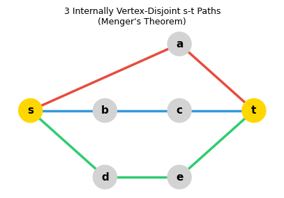
Three internally vertex-disjoint \(s\)–\(t\) paths (colored differently). Menger’s theorem guarantees this is possible whenever no set of fewer than 3 vertices separates \(s\) from \(t\).

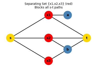
A vertex cut \(\{x_1, x_2, x_3\}\) (red) that blocks all \(s\)–\(t\) paths. Menger’s theorem says the minimum such cut size equals the maximum number of internally disjoint paths.

Menger I gives a “global” reformulation of \(k\)-connectivity in terms of disjoint paths. This is often a more useful characterization because it describes what the connectivity number means structurally — not just what removal breaks the graph, but how many independent paths exist.

Menger II is the “local” pairwise version: for any specific pair \(a, b\), the maximum number of internally disjoint paths equals the minimum size of a separator. This is the combinatorial prototype of max-flow equals min-cut.

Menger II already has an elegant min-max flavor, but it is restricted to a single pair of vertices. The most general form, Menger III, lifts this to arbitrary sets \(A\) and \(B\) — which is the version that most directly corresponds to the max-flow min-cut theorem in network flows, where \(A\) is the source set and \(B\) is the sink set.

Menger III tells us that one of the two alternatives always holds, but it is not yet a clean min-max equality — it only shows the maximum cannot exceed the minimum. The strengthened version below establishes that the two quantities are in fact equal:

The proof proceeds by induction on edges, using contraction to reduce to a smaller graph. The key idea is that any minimum separator in the contracted graph “lifts” to a minimum separator in the original — contraction cannot accidentally merge separator vertices. Together, Menger I, II, and III give a complete min-max picture of vertex connectivity.

What makes this derivation elegant is the neighborhood reduction trick: by working with the neighbors of \(a\) and \(b\) rather than \(a\) and \(b\) themselves, we convert internally-disjoint paths (a condition on internal vertices) into vertex-disjoint paths (a cleaner combinatorial condition), enabling a clean application of Menger III*.

The Fan Lemma is a useful special case of Menger III where one endpoint is a single vertex. It characterizes when a vertex “fans out” to a large set.

A fan from \(a\) to \(B\) is a collection of \(k\) paths that branch out from \(a\) and reach distinct members of \(B\) without crossing each other. The Fan Lemma is the tool used in the proof of Kuratowski’s theorem: in a 3-connected graph, fans of size 3 must exist, and their structure forces planarity or the presence of \(K_5\)/\(K_{3,3}\).

A charming corollary shows that high connectivity forces any small set of vertices to lie on a common cycle:

Chapter 4: Planar Graphs

The jump from connectivity to planarity is a jump from combinatorics to topology. Planar graphs are those that can be drawn in the plane without edge crossings. They arise naturally in geography (maps), VLSI chip design, and network layout. This chapter develops the theory around two landmark theorems: Euler’s formula (a topological identity relating vertices, edges, and faces) and Kuratowski’s theorem (a complete obstruction characterization of planarity). Together they give a remarkably complete picture of which graphs are planar and which are not.

Plane Graphs and Embeddings

A key distinction: a plane graph is a specific geometric realization in \(\mathbb{R}^2\), while a planar graph is an abstract graph that admits such a realization. A given planar graph may have many non-isomorphic plane embeddings.

Planarity is an intrinsic graph property — it does not depend on any particular drawing, only on the existence of a good one. A useful theorem (Thomassen’s) says straight-line drawings are equivalent in power to curved-edge drawings: we may assume edges are polygonal arcs without loss of generality.

The topological setting requires precise vocabulary. A curve is a subset of \(\mathbb{R}^2\) homeomorphic to \([0,1]\); it is polygonal (an arc) if it is a finite union of line segments. A closed curve (or polygon if polygonal) is the image of a continuous map \(f: [0,1] \to \mathbb{R}^2\) injective on \([0,1)\) with \(f(0) = f(1)\). The edges of a plane graph are arcs.

The distinction between the plane graph and its abstract graph reflects a fundamental tension in planarity theory: the same abstract graph may admit many non-equivalent planar embeddings, with different faces and different combinatorial structure. Whitney’s theorem (a consequence of Kuratowski’s theorem) shows that 3-connected planar graphs have essentially unique embeddings — the combinatorics locks in the topology.

Linkedness is the topological notion of connectivity in a subset of the plane. The components of \(\mathbb{R}^2 \setminus G\) under this relation are exactly the faces of \(G\) — the open regions the drawing carves out. Each face is a maximal arc-connected piece of the complement.

Once we have a plane graph, the plane is divided into regions by the drawing. These regions are the faces — the “countries” on the map.

The uniqueness of the unbounded face is intuitively obvious — the “outside” of any finite drawing is a single connected region — but it requires the Jordan Curve Theorem to make rigorous. It motivates a useful trick: by stereographic projection onto the sphere, all faces become bounded and symmetric. On the sphere, we can choose any face to serve as the “outer” face, which is why Proposition 4.7.5 (below) allows any vertex to appear on the outer face of a planar graph.

The openness of faces is a topological necessity: the boundary of each face — the edges and vertices of \(G\) that “frame” it — belongs to the graph itself, not to the face. This is why the frontier and the face are distinct notions, with the face being the open region and the frontier being its closure inside \(G\).

This is the graph-theoretic Jordan Curve Theorem: a simple closed polygon divides the plane into exactly two regions (inside and outside). It underpins all face-counting in planar graph theory. The proof uses the fact that a polygon separates any two points in different regions — any path between them must cross the polygon — which can be made rigorous using the theory of winding numbers or the intermediate value theorem.

The frontier being a genuine subgraph is the critical fact that makes face boundaries combinatorially tractable: we can count their edge lengths, apply König-style double-counting arguments, and invoke connectivity properties of the bounding subgraph. This is not obvious from the topological definition of a face as an open set — the corollary bridges the topological and combinatorial viewpoints.

Propositions 4.2.4 and 4.2.5 together set up the crucial double-counting argument for Euler’s formula: each non-bridge edge borders exactly two faces, contributing 2 to the sum of face-boundary lengths. This makes the sum \(\sum_f |\partial f| = 2|E|\) precise, which is the algebraic engine behind Euler’s formula and the edge-density bounds for planar graphs.

Faces are the topological dual of edges: just as edges separate vertices, faces are separated by edges. The unbounded face is an artifact of working in \(\mathbb{R}^2\) rather than on the sphere; projecting to the sphere would eliminate this asymmetry.

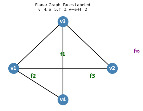
A planar graph drawn without crossings. The faces \(f_1, f_2, f_3\) are the bounded regions; \(f_\infty\) is the unbounded outer face. Here \(v=4, e=5, f=3\) and \(4-5+3=2\).

The Jordan Curve Theorem for polygons states that a circuit drawn in the plane divides it into exactly two faces. This is the topological backbone of planarity theory.

This corollary is a useful sanity check for Euler’s formula: a forest on \(n\) vertices has \(n-1\) edges and exactly 1 face, giving \(n - (n-1) + 1 = 2\) — the formula holds. The entire plane “wraps around” a forest since it has no interior, so there is really only one region surrounding all the tree branches.

A bridge, lying on only one face boundary, is a topological “spike” protruding into a single face. Non-bridge edges, by contrast, separate two distinct faces and appear on both boundaries.

Proposition 4.2.7 is the inductive step for Euler’s formula: adding a path increases \(|E|\) by the path’s length and increases \(|F|\) by exactly 1, while leaving \(|V|\) unchanged (except for the interior vertices of \(P\), which increase \(|V|\) and \(|E|\) equally). The net effect on \(v - e + f\) is always zero, preserving the invariant.

This explains why 2-connectivity is the natural hypothesis for many planar graph results: it ensures faces are “well-shaped” — bounded by genuine cycles rather than paths or trees.

Euler’s Formula

With vertices, edges, and faces all defined, we can now state and prove the single most important fact about plane graphs. Euler’s formula is the fundamental identity relating the combinatorial structure of a planar graph to its topology. Discovered by Euler in 1752, it was one of the first theorems in topology.

Euler’s formula says that the quantity \(v - e + f\) (the Euler characteristic) is a topological invariant: it equals 2 for any connected plane graph, regardless of which graph it is or how it is drawn.

The proof peels off edges one at a time, starting from any spanning tree (which satisfies the formula trivially) and adding edges back, each time increasing both \(|E|\) and \(|F|\) by one so their contribution cancels. The formula is the origin of all the edge-count bounds that make planarity so powerful as a structural hypothesis.

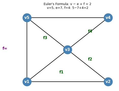
\(v=5\), \(e=7\), \(f=4\) (including the outer face): \(5-7+4 = 2\). Euler’s formula holds.

This proposition is the bridge between the topological world of faces and the combinatorial world of cycles. A face boundary that contains a cycle means the face is “enclosed” by that cycle — the Jordan Curve Theorem applies, and the face lies in one of the two regions created by the cycle. This is exactly the situation needed to apply the double-counting argument for Euler’s edge-density bound: faces with cycle boundaries contribute at least 3 to the face-edge count, while faces with tree boundaries contribute fewer edges but are handled separately.

A powerful consequence of Euler’s formula is an edge count bound — planarity severely limits how many edges a graph can have.

The proof is a double-counting argument on face-edge incidences, combined with Euler’s formula to translate a face count into an edge bound. The edge density bound \(|E| \leq 3|V| - 6\) is one of the most practically useful facts about planar graphs: it immediately certifies non-planarity by comparing edge counts alone.

This corollary is the key step toward Kuratowski’s theorem: \(K_5\) and \(K_{3,3}\) are non-planar by pure counting. The deep result ahead is that these are the only “minimal” non-planar graphs.

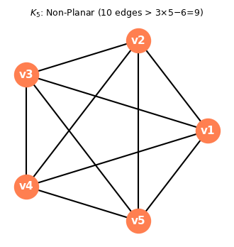
\(K_5\) has 10 edges, exceeding the bound \(3 \times 5 - 6 = 9\). It cannot be planar.

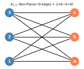
\(K_{3,3}\) is triangle-free with 9 edges, exceeding the bound \(2 \times 6 - 4 = 8\). It cannot be planar.

Subdivisions and Graph Minors

To make Kuratowski’s theorem precise, we need two ways of “containing” a graph inside another: subdivisions (inserting degree-2 vertices into edges) and minors (contracting edges). Both preserve non-planarity — if a non-planar graph appears inside \(G\) in either sense, then \(G\) itself cannot be planar.

Think of a topological minor as a “stretched copy” of \(H\) living inside \(G\): the edges of \(H\) are replaced by longer paths, but the high-degree branching structure is preserved. The key insight is that subdivision does not change whether a graph is planar — you can always place new degree-2 vertices in the interior of an edge without introducing crossings. So if \(H\) is non-planar, any graph containing a subdivision of \(H\) as a subgraph is also non-planar.

Subdividing an edge introduces degree-2 “relay” vertices but preserves the drawing topology: if \(H\) cannot be drawn without crossings, neither can any subdivision of \(H\). The Petersen graph, for instance, contains a subdivision of \(K_{3,3}\) as a subgraph, proving it non-planar.

The functional characterization in Proposition 4.6.2 makes the topological minor relation tractable for algorithmic purposes: instead of searching through all possible subdivisions, we look for a mapping of vertices to terminals and edges to internally disjoint paths. This is exactly the structure a planarity algorithm needs to exhibit when certifying that a non-planar graph contains a \(K_5\) or \(K_{3,3}\) subdivision.

Minors are more general than subdivisions: a contraction can merge vertices of arbitrarily high degree, whereas a subdivision only affects degree-2 vertices. The distinction is important for the equivalence stated next.

The distinction between topological minors (subdivisions) and minors (contractions) is subtle but important. Topological minors are the more restrictive notion:

The converse is false in general: having \(H\) as a minor does not imply having \(H\) as a subdivision. However, for \(K_5\) and \(K_{3,3}\) specifically, the two notions coincide.

The proof uses the fact that both \(K_5\) and \(K_{3,3}\) have maximum degree \(\leq 4\) and \(3\) respectively, so their minors can be “expanded” back into topological copies. This equivalence is what makes the formulation of Kuratowski’s theorem in terms of either minors or subdivisions equally valid.

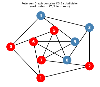
The Petersen graph contains a subdivision of \(K_{3,3}\) (red terminals). This proves the Petersen graph is non-planar via Kuratowski’s theorem.

Kuratowski’s Theorem

The proof of Kuratowski’s theorem uses two key lemmas about circuits and vertex sets on those circuits.

The \(A\)-interval is simply an arc of the cycle \(C\) delimited by consecutive members of \(A\). When two vertex sets \(A\) and \(B\) both mark points on the cycle, the relative positions of these marks — whether they interleave or nest — determine whether a \(K_5\) or \(K_{3,3}\) minor is forced. This is exactly what the Circle Lemma classifies.

The Circle Lemma is the technical core of the proof of Lemma 4.7.4: given neighbors of the two ends of a contracted edge lying on a facial circuit, the four outcomes correspond to a small separator (contradicting 3-connectivity), a \(K_5\) minor, a \(K_{3,3}\) minor, or a valid planar embedding.

All the machinery of this chapter — Euler’s formula, minors, subdivisions, Tutte’s Wheel Theorem, and the Fan Lemma — converges on one theorem. Kuratowski’s theorem (1930) gives a complete characterization of planar graphs — arguably the most celebrated theorem in graph theory.

The theorem says that \(K_5\) and \(K_{3,3}\) are the only “minimal” obstructions to planarity: every non-planar graph contains one of them in disguise. This is a profound combinatorial fact — there are infinitely many non-planar graphs, yet they all share a finite set of witnesses.

The key step is the 3-connected case, which uses Tutte’s Wheel Theorem as its inductive engine:

The proof strategy is a minimal counterexample argument combined with Tutte’s theorem: contract an edge to get a smaller 3-connected graph, embed it by induction, then “uncontracting” the edge must either work (giving a planar embedding) or reveal a forbidden minor. The Circle Lemma is the technical tool that classifies all cases.

For the general (not necessarily 3-connected) case, one reduces to the 3-connected case by showing that non-3-connected planar graphs can be built from planar pieces:

This lemma is used in the proof of Theorem 4.5.2: adding a vertex inside a face and connecting it to the boundary preserves planarity, and allows the Circle Lemma to be applied.

Facial Circuit Characterization for 3-Connected Graphs

This is a purely combinatorial characterization — it does not depend on the choice of planar embedding! For 3-connected planar graphs, the embedding is essentially unique (by Whitney’s theorem), so the facial circuits are combinatorially determined.

Algorithmic Planarity Testing

Planarity can be tested in \(O(n)\) time (Hopcroft-Tarjan, 1974). The approach in these notes is:

1. Check if G is 3-connected (O(n²) via pairwise vertex deletion + BFS).
2. If G is 3-connected:
   a. Find edge e such that G/e is 3-connected (Tutte's theorem guarantees existence).
   b. Recursively test G/e.
   c. If G/e is planar, use Circle Lemma to either find a K5/K33 minor or embed G.
3. If not 3-connected:
   a. Handle cut vertices and 2-separators by splitting into simpler pieces.
   b. Embed pieces separately and combine using Proposition 4.7.5.

Straight-Line Embeddings

The spring embedding is constructed as a linear system: fix the outer face as a convex polygon, then set each interior vertex to the average (centroid) of its neighbors’ positions. This system has a unique solution, and Tutte’s theorem proves the resulting drawing is planar with convex faces. The name “spring embedding” comes from a physical analogy: imagine replacing every edge with an ideal spring of unit stiffness and natural length zero — the equilibrium configuration of the spring system is exactly the centroid condition, and the unique equilibrium is the unique solution to the linear system.

The proof proceeds via four key lemmas about the geometry of the spring embedding. The logic is layered: Lemma I gives a local balancing property for every interior vertex, Lemma II lifts this to a global connectedness statement, Lemma III rules out the degenerate case where neighbors collapse onto a line, and Lemma IV uses the circuit structure to separate adjacent faces. Together they force the faces to be genuine convex polygons with disjoint interiors.

The key insight here is the centroid condition: if \(\varphi(u)\) is the average of its neighbors’ positions, then \(\varphi(u)\) lies in the convex hull of its neighbors. Any line through \(\varphi(u)\) must therefore have neighbors on both sides — otherwise the centroid would be pushed off that line, a contradiction.

This connectivity-in-half-planes property is what guarantees the drawing does not “fold back” on itself. It is a global consequence of the local balancing: no subset of embedded vertices can be isolated in a half-plane unless they are already isolated in the graph, which 3-connectivity rules out.

Lemma III rules out the degenerate scenario where all neighbors of an interior vertex collapse onto a single line. This would cause the embedding to be “flat” at \(u\) — all neighbors on one line means the faces meeting at \(u\) have no angular separation, and the drawing folds. The proof uses the 3-connectivity of \(G\): if all neighbors of \(u\) lay on a line, the half-plane connectivity of Lemma II would be violated. This is where the 3-connectivity hypothesis does its deepest work in the entire proof.

Lemma IV is where the combinatorial structure of the planar graph meets the geometry of the embedding: adjacent faces, sharing an edge, are separated by the line through that edge’s endpoints. This is what ensures the drawing is crossing-free — no two face interiors overlap.

Together these lemmas establish that the spring embedding produces a valid straight-line plane drawing with all faces convex. What makes this remarkable is that convexity is achieved purely from the linear system — no geometric optimization is needed; the equilibrium condition of the spring system automatically produces a convex embedding, a beautiful interplay between linear algebra and graph topology.

Dual Graphs

Every plane graph has a natural “mirror image” — its plane dual — where faces become vertices and edges connect faces that share a boundary. This duality swaps the roles of faces and vertices, turning cuts into cycles and cycles into cuts. It is one of the most beautiful correspondences in graph theory.

Given a plane graph \(G\), its plane dual \(G^*\) is constructed as follows: for each face \(f\) of \(G\), place a vertex \(f^*\) inside that face; for each edge \(e\) of \(G\) shared by faces \(f\) and \(g\), draw an edge \(e^*\) connecting \(f^*\) and \(g^*\), crossing only the edge \(e\). The result is another plane graph, with one vertex per face of \(G\) and one edge per edge of \(G\).

Two immediate observations: (1) loops arise in \(G^*\) when \(e\) is a cut edge of \(G\) (both sides of \(e\) are in the same face after removing \(e\)); (2) multiple edges arise when two faces share more than one boundary edge. So even if \(G\) is simple, \(G^*\) may have loops and multiple edges.

The planarity of \(G^*\) is immediate from the construction: we explicitly drew it in the plane without crossings. The double-dual identity holds for connected plane graphs but fails for disconnected ones: a disconnected plane graph has a connected dual (since any two face-vertices are connected through the outer face), but the dual of that connected dual cannot recover the original disconnected graph.

The dual construction respects the operations of deletion and contraction in a beautifully symmetric way:

In words: deleting an edge from \(G\) corresponds to contracting its dual edge in \(G^*\), and vice versa. This is a perfect duality of operations: the two “simpler” operations — edge deletion and edge contraction — are swapped by the dual. It implies that the class of planar graphs is closed under both deletion and contraction, a key ingredient in the proof of Kuratowski’s theorem via the minor relation.

The deepest connection between a graph and its dual involves cycles and cuts. A cycle in \(G\) separates the plane into an interior and exterior, so the faces inside and outside the cycle each form a connected set. This means the corresponding edges in \(G^*\) form a bond (a minimal cut):

The intuition for the first statement: a cycle \(C\) encloses a region of the plane; the faces inside and outside form two connected sets, and the edges of \(G^*\) crossing \(C\) are exactly those separating these two sets — a bond. The algebraic formulation says the cycle and cut spaces swap roles under duality, which is a profound structural symmetry.

This suggests a purely combinatorial notion of “dual” that does not require a planar embedding. Two graphs \(G\) and \(H\) on the same edge set are abstract duals if every cycle in \(G\) is a bond in \(H\) and every bond in \(G\) is a cycle in \(H\). Connected plane graphs and their plane duals are abstract duals, but the definition applies to any pair of graphs. Whitney’s theorem (1932) characterizes exactly which graphs have abstract duals:

This is yet another characterization of planarity — this time in terms of the algebraic relation between cycles and bonds. The forward direction follows from the plane dual construction above. The reverse uses MacLane’s theorem (below): if \(G\) has an abstract dual \(G^*\), then the cycle space of \(G\) equals the cut space of \(G^*\), and the cuts of any graph are spanned by the \(\delta(v)\) (the edge-cuts at individual vertices), each edge appearing in at most two such cuts — giving a 2-basis for the cycle space of \(G\), hence \(G\) is planar by MacLane’s theorem.

MacLane’s Theorem

Kuratowski’s theorem characterizes planar graphs by what they cannot contain (no subdivision of \(K_5\) or \(K_{3,3}\)). MacLane’s theorem (1937) characterizes planarity positively — by a special algebraic property of the cycle space. It says that a graph is planar if and only if its cycle space has a particularly efficient spanning set.

Recall that the cycle space \(\mathcal{C}(G)\) is the subspace of the edge space over \(\mathbb{F}_2\) spanned by all cycles. A 2-basis for a subspace is a basis where each edge of \(G\) appears in at most 2 of the basis elements.

The motivation for this definition comes from plane graphs: in any 2-connected plane embedding, the facial cycles — the cycles bounding the faces — span the cycle space (as we showed via fundamental cycles of the dual spanning tree), and every edge borders exactly 2 faces, so the facial cycles form a 2-basis. MacLane’s theorem says this property characterizes planarity:

The forward direction follows from plane graphs: embed \(G\) in the plane, take any 2-connected block, and use its facial cycles as the 2-basis (every edge borders exactly 2 faces). For disconnected graphs, combine the 2-bases of each block.

The reverse direction requires more work. The key idea is to use Wagner’s theorem: if \(G\) is not planar, then \(G\) has \(K_5\) or \(K_{3,3}\) as a minor. The proof then shows two things:

1. The 2-basis property is inherited by minors. If the cycle space of \(G\) has a 2-basis, then so does the cycle space of any minor of \(G\). This is proved by tracking how a 2-basis transforms under each minor operation: removing an isolated vertex does not change the edge set; deleting an edge either removes a non-essential basis element or reduces the dimension by one; contracting an edge modifies each basis element containing the contracted edge by removing it, and the parity constraints are preserved.

2. \(K_5\) and \(K_{3,3}\) do not have 2-bases. For \(K_5\): the cycle space has dimension \(|E| - |V| + 1 = 10 - 5 + 1 = 6\). If \(\{B_1, \ldots, B_6\}\) were a 2-basis, form \(B_7 = B_1 \oplus \cdots \oplus B_6\). Now \(B_7\) contains exactly the edges appearing in an odd number of basis elements. The collection \(B_1, \ldots, B_7\) together contains each of the 10 edges exactly twice (2-basis condition), so \(20\) edge-appearances total. But \(7\) elements with \(\geq 3\) edges each would require \(\geq 21\) appearances — a contradiction by the pigeonhole principle. For \(K_{3,3}\), a similar dimension argument works.

Combining: if \(G\) is not planar, it has \(K_5\) or \(K_{3,3}\) as a minor; those do not have 2-bases; hence \(G\) does not have a 2-basis either (since the property is preserved under taking minors).

MacLane’s theorem is remarkable because it translates a topological property (embeddability in the plane) into a purely algebraic statement about a vector space. The 2-basis condition is checkable in polynomial time: one can compute a basis for the cycle space and test whether each edge appears at most twice. This gives an algebraic planarity algorithm complementary to Kuratowski’s combinatorial criterion.

Chapter 5: Matchings (Advanced)

The bipartite matching theory of Chapter 1 — Hall’s theorem, König’s theorem — relied on the absence of odd cycles. In general graphs, odd cycles create an obstruction that has no bipartite analogue: they prevent perfect matchings in a fundamentally different way. This chapter develops the matching theory for general graphs, building toward Edmonds’ celebrated Blossom Algorithm (1965), which was one of the first examples of a polynomial-time algorithm for a seemingly difficult combinatorial problem.

Chapter 5 re-develops the matching vocabulary in the general (non-bipartite) setting, then builds toward the Tutte-Berge formula and the Blossom Algorithm. The key obstacle that makes general matching harder than bipartite matching is the existence of odd cycles: a single triangle prevents a perfect matching on 3 vertices, and the pattern generalizes. The theory must somehow quantify and account for this parity obstruction.

The Chapter 1 definitions are re-stated here in the general (non-bipartite) setting because the subsequent theory demands precision: the notions of saturation and exposure are exactly what augmenting paths and blossoms interact with. In bipartite graphs, Berge’s augmenting path theorem sufficed algorithmically. In general graphs, the same theorem holds (Proposition 5.4.5 below), but finding augmenting paths becomes much subtler because odd cycles create “fake dead ends” in any straightforward BFS search.

Matchings and vertex covers are dual problems: one packs as many vertex-disjoint edges as possible, the other selects the fewest vertices to “guard” all edges. The fact that \(\nu \leq \tau\) is trivial — every vertex in the cover must hit every matching edge, and matching edges are disjoint. The non-trivial question is whether equality holds, and the answer depends crucially on the bipartiteness of the graph.

Proposition 5.2.2 gives a certificate of optimality: if you exhibit a matching and a cover of the same size, you have simultaneously proved both are optimal without needing to check any other matchings or covers. This “primal-dual” certificate is the foundation of LP duality applied to matchings.

Notice that this proof of König’s theorem via Menger’s theorem is far more elegant than the direct proof in Chapter 1: it reveals that König’s theorem and Menger’s theorem are the same result in different guises — both are min-max equalities arising from the same underlying flow argument. This connection foreshadows the relationship between maximum matching and maximum flow in networks.

2-Factors and Factorizations

A 1-factor of \(G\) is a perfect matching — a spanning 1-regular subgraph. A \(k\)-factor is a spanning \(k\)-regular subgraph: every vertex has degree exactly \(k\) in the subgraph. A 2-factor is therefore a spanning 2-regular subgraph, which must consist of a collection of disjoint cycles covering all vertices.

Before tackling general factors, notice that Hall’s theorem immediately gives a structural result for regular bipartite graphs:

The existence of a 1-factorization means the edges of a regular bipartite graph can be properly edge-colored with \(k\) colors — this is a restatement of König’s edge-coloring theorem. For example, a schedule of a round-robin tournament with \(2n\) teams can be constructed by 1-factorizing the complete bipartite graph \(K_{n,n}\).

The 2-factor theorem extends this to non-bipartite regular graphs:

The proof is beautifully indirect, using Eulerian circuits and a bipartite “split” construction. The key insight is that a 2k-regular graph has an Eulerian circuit, and this circuit can be converted into a bipartite graph that is k-regular — to which Proposition 5.2.4 applies.

The proof uses a double encoding: first translate the graph problem into an Eulerian circuit problem, then encode the circuit as a bipartite graph to access the power of Hall’s theorem. This is a characteristic technique in combinatorics — “reducing” a hard problem to one we already know how to solve by changing representation.

Examples. The complete graph \(K_{2n}\) is \((2n-1)\)-regular; since \(2n-1\) is odd, it does not have a 2-factorization directly, but a 1-factorization exists (by extending the bipartite case). The complete graph \(K_{2n+1}\) is \(2n\)-regular and does have a 2-factorization into \(n\) Hamiltonian cycles — this is the basis for round-robin tournament scheduling where every round is a Hamiltonian tour. The Petersen graph is 3-regular; it has no 2-factor (for parity reasons: \(|V| = 10\) but the Petersen graph has no perfect matching in certain induced subgraphs), and Tutte’s theorem precisely characterizes when this failure occurs.

General Matchings and the Tutte-Berge Formula

In Chapter 1 we handled bipartite matchings via Hall’s theorem. For general (non-bipartite) graphs, the situation is more complex because odd cycles prevent perfect matchings in a subtle way. The right generalization of Hall’s condition involves counting odd components of the graph after removing vertices.

The key insight is that odd components must “borrow” at least one matching edge from the set \(S\), but \(S\) only has \(|S|\) edges to give. When there are too many odd components, the supply is exhausted.

For two matchings \(M, M'\), the symmetric difference \(G[M \cup M']\) (the graph on vertex set \(V(G)\) with edge set \(M \cup M'\)) consists only of paths and even circuits, since every vertex has degree at most 2. This observation leads to:

The symmetric difference \(M \triangle M'\) of two matchings is the structural bridge between them. Since every vertex has degree at most 1 in each matching, it has degree at most 2 in their union — so the components of \(G[M \triangle M']\) are paths and cycles. The cycles must be even (alternating matching edges force this). This decomposition is the core tool for proving that augmenting paths exist whenever a matching is non-maximum: if \(|M'| > |M|\), there must be more \(M'\)-edges than \(M\)-edges in the symmetric difference, which forces at least one path component to start and end with \(M'\)-edges — an \(M\)-augmenting path.

Tutte’s theorem (1947) shows this necessary condition is also sufficient — a remarkable achievement that took over a decade after Hall’s theorem to establish:

Tutte’s theorem is the complete analogue of Hall’s theorem for general graphs: where Hall’s asks about neighborhood sizes in a bipartite graph, Tutte’s asks about odd component counts after vertex deletion. Both give an “if and only if” characterization with a single combinatorial obstruction.

The Tutte-Berge formula generalizes this to compute the exact size of a maximum matching — not just whether a perfect one exists, but how large any maximum matching can be:

The Tutte-Berge formula gives the exact matching number as an optimization over all vertex subsets — a min-max theorem in the spirit of König’s theorem, but for arbitrary graphs. The minimizing set \(S\) is called a Berge witness or Tutte-Berge witness. It certifies that no larger matching can exist: the formula says we have exactly \(\frac{1}{2}(\text{odd}(G-S) - |S|)\) unmatched vertices in any maximum matching.

A Berge witness is a certificate of matching size analogous to a vertex cover in König’s theorem: it proves the matching cannot be improved, with no need to enumerate all matchings. Notice that \(S = \emptyset\) is always a valid witness (giving the lower bound \(\nu(G) \geq \frac{1}{2}|V(G)| - \frac{1}{2}\text{odd}(G)\)), but the tightest witness is the one minimizing the right-hand side — which turns out to be the set \(A(G)\) from the Gallai-Edmonds partition.

A classical consequence of Tutte’s theorem that seemed surprising when first proved in 1891:

The proof is a counting argument: regularity forces enough edges from odd components to \(S\) to verify Tutte’s condition. The absence of cut edges provides the lower bound of 3 edges per odd component, making the counting work.

Matching Structure: Gallai-Edmonds

The Tutte-Berge formula tells us the size of a maximum matching. The Gallai-Edmonds decomposition (independently by Gallai and Edmonds, 1960s) goes further, giving the complete structural picture of which vertices can be left unmatched and how the matching edges are arranged globally.

Avoidable vertices are the “optional” ones: we can always find a maximum matching that leaves them unmatched. They form the \(D\) set in the Gallai-Edmonds partition.

The partition \(D, A, C\) stratifies the vertex set by their matching behavior: \(D\) vertices are avoidable, \(A\) vertices are the “interface” between avoidable and unavoidable regions, and \(C\) vertices are always matched in every maximum matching.

This theorem gives a complete and canonical description of the bottleneck structure of maximum matchings in any graph. It reveals that the worst witness \(S\) in the Tutte-Berge formula is always \(A(G)\) — the neighborhood of the “deficiency” region.

Hypomatchable graphs are the “building blocks” of the \(D\) set: they can be matched perfectly except for any single specified vertex, which makes them structurally very flexible.

The proof uses a clever “twin relation” \(u \sim v\) defined by \(\nu(G - \{u,v\}) < \nu(G)\), showing it is an equivalence relation (the non-trivial part is transitivity), then analyzing the equivalence classes.

Lemma 5.4.2 is the hardest step: it shows that the odd components left over by the “canonical” witness \(\hat{A}\) are not just odd — they are hypomatchable, meaning they can absorb the loss of any single vertex while maintaining near-perfect matching. The proof uses the twin relation from Lemma 5.3.4 and a careful exchange argument: if a non-hypomatchable odd component existed, we could modify \(\hat{A}\) to reduce the number of such components, contradicting its minimality. It is a beautiful argument by contradiction that forces the worst-case structure to be maximally structured.

Lemma 5.4.3 is the “expansion” condition for the set \(\hat{A}\): every subset of \(\hat{A}\) has strictly more neighboring odd components than its own size. This is a Hall-like condition in reverse — instead of asking about neighborhoods in a bipartite graph, we ask about odd components accessible to a subset of \(\hat{A}\). The excess “+1” ensures that after matching the odd components to \(\hat{A}\), exactly one vertex in each odd component remains unmatched — the vertex “left out” for each hypomatchable component.

Lemma 5.4.4 completes the identification of \(D(G)\): it shows that every vertex in the odd components of \(G - \hat{A}\) can be left unmatched by some maximum matching. Combined with Lemma 5.4.2 (which shows those components are hypomatchable), this gives precise control: for any vertex \(v\) in an odd component, the hypomatchable structure supplies a matching of that component leaving \(v\) out, and the rest of the graph can be matched to accommodate this choice.

These three lemmas together establish that \(\hat{A} = A(G)\), proving the Gallai-Edmonds Theorem.

This is Berge’s theorem restated in the general (non-bipartite) setting — it is the key algorithmic tool showing that searching for augmenting paths is equivalent to finding a maximum matching.

The Blossom Algorithm

The theory is now rich enough to support an efficient algorithm. In bipartite graphs, BFS augmenting paths suffice. In general graphs, odd cycles (“blossoms”) confuse the augmenting path search — they create false cycles in the alternating-path structure. Edmonds’ genius was to handle this by contracting blossoms: an odd cycle can be treated as a single vertex without affecting the existence of augmenting paths.

The Blossom Algorithm (Edmonds, 1965) finds a maximum matching in a general graph in polynomial time — a landmark in combinatorial optimization.

The inner/outer distinction is the core algorithmic insight. Outer vertices are “reachable from the root by even alternating paths” — they are the candidates for the next step of an augmenting path. Inner vertices serve only as “connectors” through matching edges and cannot be extended from. An edge from an outer vertex to an exposed vertex immediately gives an augmenting path; an edge between two outer vertices in different trees also gives an augmenting path. The only problematic case is an edge between two outer vertices in the same tree — this is exactly where a blossom forms.

A blossom is the culprit behind the difficulty of general matching: it is an odd cycle that is “almost matched” internally, with one vertex sticking out as the unsaturated root. When the augmenting path search reaches this cycle, it is confused — there appear to be two alternating paths entering the cycle, but they are actually the same path traversing the cycle in opposite directions. Edmonds’ brilliant resolution is to shrink the blossom to a single supervertex, solve the matching problem on the contracted graph, and then “lift” the solution back: the one unsaturated vertex of the blossom can be chosen to be whichever member of the cycle allows the lifted augmenting path to work.

An alternating tree is the search structure for finding augmenting paths: we grow the tree outward from an exposed vertex, alternating matching and non-matching edges. Outer vertices are “reachable by even-length alternating paths” — potential starting points for augmentations.

Input: Graph G, initial matching M (possibly empty).
Output: A maximum matching M*.

1. Build an M-alternating forest F rooted at all exposed vertices.
2. For each outer vertex u and edge uv:
   a. If v is exposed: we found an augmenting path → augment M, restart.
   b. If v is an outer vertex in a different tree: augmenting path found → augment M, restart.
   c. If v is an outer vertex in the SAME tree:
      → Found a blossom B (odd cycle). Contract B to a single vertex.
      → Recursively find an augmenting path in G/B.
      → Lift the path back to G (expand the blossom).
   d. If v is an inner vertex: ignore (already handled).
3. If no augmenting path found: M is maximum (by Berge's theorem).

The subtle case (2c) is the “blossom” contraction — the key insight that makes the algorithm work for non-bipartite graphs. Without it, odd cycles would confuse the alternating path search. After contracting a blossom to a single vertex, any augmenting path in the contracted graph can be “lifted” back to an augmenting path in the original graph — this lifting is non-trivial and is the core of Edmonds’ contribution.

These two propositions together give the blossom contraction step: whenever an edge between same-tree outer vertices is found, the resulting blossom can be contracted and the algorithm recurses. Since matching size is at most \(\frac{1}{2}|V(G)|\), the recursion depth is \(O(|V(G)|)\), giving a polynomial-time algorithm.

Slither: A Game-Theoretic Application

The Gallai-Edmonds structure has a beautiful application to combinatorial game theory via the game of Slither: two players alternately extend a path by choosing an adjacent edge; the player who cannot move loses.

The strategy here is elegant: Alice uses the matching as a “script.” Whenever Bob adds vertex \(v\) to the path, Alice’s response is predetermined — she follows the matching edge from \(v\) to its partner, extending the path into a vertex that still has a matched partner available. Since the matching is perfect, Bob can never get stuck first; it is always Alice who has a legal move. This is the matching strategy technique, a beautiful interplay between combinatorial structure and game-theoretic reasoning.

The hypomatchable case is the dual: Bob waits for Alice to commit a vertex, then uses the perfect matching of \(G - v\) (which exists by hypomatchability) as his script. No matter which vertex \(v\) Alice moves to first, Bob’s matching of the remaining graph always gives him a response. Thus Alice must eventually get stuck. The two strategies together show the Gallai-Edmonds partition completely determines who wins Slither.

Propositions 5.5.3 and 5.5.4 together handle the mixed case: when the graph has both a \(C\) region (always matched) and a \(D\) region (avoidable), the game becomes a territorial contest. Vertices in \(C(G)\) are “safe” to traverse because the matching structure guarantees a continuation; venturing into \(D(G)\) is the fatal move. Alice, moving first, can exploit the \(C\) region to stay in safe territory and force Bob to be the one who must eventually enter \(D(G)\).

When \(C(G) = \emptyset\), the analysis reduces recursively to the Gallai-Edmonds partition of \(A(G)\), and so on.

This elegant application shows how matching theory reaches into other areas of combinatorics — a hallmark of the subject’s depth.

Chapter 6: Bonus Material

Having developed the combinatorial and topological core of graph theory, we turn to three bonus topics that illustrate the breadth of the subject: extremal graph theory (how dense can a graph be without containing a given subgraph?), algebraic graph theory (how does linear algebra encode graph structure?), and counting (how many spanning trees does a graph have?). The last of these leads to two of the most beautiful formulas in combinatorics: Kirchhoff’s Matrix-Tree Theorem and Cayley’s formula \(n^{n-2}\) for labeled trees.

Extremal Graph Theory

A classic open question: does there exist a graph with chromatic number 100 but girth (shortest cycle length) at least 1000? The answer is yes — this follows from probabilistic arguments — but constructing explicit examples is non-trivial. This is the flavor of extremal graph theory: bounding global parameters in terms of local structure.

Algebraic Graph Theory

Graph theory and linear algebra speak different languages — one combinatorial, one algebraic — but they share a remarkable grammar. The edge structure of a graph can be encoded as a vector space over \(\mathbb{F}_2 = \{0,1\}\), the field with two elements, where addition is modulo 2. Within this space, two fundamental subspaces emerge: the cut space (capturing all cut-sets) and the cycle space (capturing all even subgraphs). These spaces are orthogonal complements of each other, and their interplay encodes planarity, spanning trees, and much more.

The Edge Space

The edge space of \(G\), denoted \(\mathcal{E}(G)\), is the vector space \(\mathbb{F}_2^{E(G)}\) — the set of all binary vectors indexed by the edges. Each vector \(f \in \mathcal{E}(G)\) can be identified with a spanning subgraph of \(G\): edge \(e\) is included if and only if \(f_e = 1\). Under this identification, vector addition corresponds to the symmetric difference of edge sets: \(f_1 + f_2\) contains the edges in exactly one of \(f_1\) or \(f_2\). Scalar multiplication is trivial since \(\mathbb{F}_2 = \{0,1\}\).

Since the edge space has dimension \(|E(G)|\) (the standard basis is the set of individual edges), the combinatorial “size” of a graph is directly captured by the dimension of its edge space. The interesting structure lies not in the whole space, but in special subspaces.

Cut Space and Fundamental Cuts

The cut space is indeed a subspace: the symmetric difference of two cuts is again a cut, since \(\delta(S_1) \oplus \delta(S_2) = \delta(S_1 \triangle S_2)\). The zero vector is the empty cut \(\delta(\emptyset)\).

What spans the cut space? Every cut is a disjoint union of bonds (minimal cuts), so the set of all bonds spans \(\mathcal{C}^*(G)\). To find a basis, we use spanning trees.

The dimension formula \(|V| - k\) counts the edges of a spanning forest, which is precisely the number of fundamental cuts. For a connected graph, this is \(|V| - 1\).

Cycle Space and Fundamental Cycles

The equivalence deserves explanation. Every cycle is even (each internal vertex has degree 2, the endpoints have degree 0 in the subgraph). The symmetric difference of two even subgraphs is even, so the cycle space is closed under addition. Conversely, every even subgraph can be decomposed into edge-disjoint cycles (by repeatedly finding and removing cycles), so it lies in the span of all cycles.

The proof mirrors the cut space argument: each non-tree edge \(e\) appears only in its own fundamental cycle \(C_T(e)\), giving linear independence; and any even subgraph can be expressed as a symmetric difference of fundamental cycles corresponding to its non-tree edges.

The dimension \(|E| - |V| + k\) is called the circuit rank or cyclomatic number of \(G\). It counts the “independent cycles” — the degrees of freedom remaining after spanning the graph with a forest.

Orthogonal Complement: Cut Space and Cycle Space are Perpendicular

The cut space and cycle space are not just two subspaces — they are orthogonal complements of each other. Define the inner product of two edge sets \(F_1, F_2\) over \(\mathbb{F}_2\) as \(\langle F_1, F_2 \rangle = |F_1 \cap F_2| \pmod{2}\): it is 0 if they share an even number of edges, and 1 otherwise.

This theorem is a direct algebraic reflection of the geometric fact that in a plane graph, cuts separate regions while cycles enclose them — two orthogonal notions. The dimension check confirms it: \(\dim \mathcal{C}^* + \dim \mathcal{C} = (|V| - k) + (|E| - |V| + k) = |E| = \dim \mathcal{E}(G)\), exactly as the orthogonal complement theorem from linear algebra requires.

For planar graphs, the dual graph construction provides a vivid geometric explanation: the cycle space of \(G\) equals the cut space of \(G^*\) (Theorem 4.10.3), and vice versa. Algebraic duality and geometric duality are the same thing.

This duality between cuts and cycles in planar graphs is a beautiful algebraic reflection of the geometric dual construction. The cut space and cycle space are orthogonal complements of each other (over \(\mathbb{F}_2\)), with the planar dual swapping the roles of the two spaces.

Bases of the Incidence Matrix

Total unimodularity is a powerful property with far-reaching algorithmic consequences: it guarantees that every linear program with a totally unimodular constraint matrix has an integer optimal solution. For graphs, this means matching and flow problems can be solved by LP relaxation without worrying about integrality — the linear programming solution is automatically an integer. König’s theorem and the Max-Flow Min-Cut theorem can both be understood as consequences of total unimodularity of the appropriate incidence matrix.

This theorem (Seymour, 1980) is the matroid-theoretic analogue of Kuratowski’s theorem: it classifies the “building blocks” of all regular matroids, just as Kuratowski classified the obstructions to planarity. A regular matroid is one representable over every field, which includes all graphic matroids (the matroids of forests). The decomposition into graphic, cographic, and the exceptional \(R_{10}\) (the matroid of the Petersen graph) gives a complete structural picture with deep algorithmic implications.

The Laplacian is a central object in spectral graph theory. Its eigenvalues encode deep graph properties: the second-smallest eigenvalue (the “algebraic connectivity” or Fiedler value) measures how well-connected the graph is, the spectrum determines the number of spanning trees (via the Matrix-Tree Theorem), and the eigenvectors give optimal graph partitions and embeddings — including, remarkably, the Tutte spring embedding from Chapter 4. The formula \(L = BB^T\) makes clear that \(L\) is positive semidefinite, with the all-ones vector always in its null space (since every row sums to zero), corresponding to the connectivity condition.

The Cauchy-Binet formula is the algebraic engine behind the Matrix-Tree Theorem. Applied to \(B\) (with a row deleted), each square submatrix of \(B\) corresponds to a subset of \(n-1\) edges, and its determinant is \(\pm 1\) if those edges form a spanning tree and \(0\) otherwise (by Proposition 6.3.1). So the sum of squares over submatrices counts spanning trees. What makes this remarkable is that a purely algebraic identity — a formula for a matrix determinant — becomes a combinatorial counting statement when the matrix is the incidence matrix of a graph.

The Matrix-Tree Theorem (Kirchhoff, 1847) is one of the oldest results in algebraic combinatorics, predating modern graph theory itself. Kirchhoff proved it to analyze electrical circuits: the number of spanning trees governs the resistance of a network. What is astonishing is that a single determinant — a number computed by Gaussian elimination — encodes the entire count of spanning trees, which seems to require exponential enumeration. The key insight is that the Laplacian’s minors count spanning trees via Cauchy-Binet, converting a global combinatorial question (how many spanning trees?) into a local algebraic computation (what is this determinant?).

Cayley’s formula \(n^{n-2}\) is one of the most striking formulas in combinatorics. For \(n = 4\), there are \(4^2 = 16\) labeled spanning trees of \(K_4\) — one can verify this by enumeration. For \(n = 10\), the count is already \(10^8 = 100{,}000{,}000\). The formula can be proved in at least four different ways: by the Matrix-Tree Theorem (as above), by a direct bijection with sequences of length \(n-2\) (Prüfer sequences), by a double-counting argument due to Cayley himself, or by a recursive identity. The Prüfer sequence bijection is perhaps the most enlightening: it shows that a labeled tree on \(n\) vertices is determined by a sequence of \(n-2\) “parent choices,” each independently ranging over \(n\) options, giving exactly \(n^{n-2}\) trees.

These notes cover CO 342 Graph Theory as taught at the University of Waterloo in Fall 2019. The major theorems covered are: Hall’s Marriage Theorem, König’s Theorem, Menger’s Theorem, Tutte’s Wheel Theorem, Euler’s Formula, Kuratowski’s Theorem, Fáry’s Theorem, Tutte’s Spring Theorem, Tutte’s Perfect Matching Theorem (Tutte-Berge Formula), Petersen’s Theorem, and the Gallai-Edmonds Decomposition.