CO 255: Introduction to Optimization (Advanced)

These notes are based on Felix Zhou’s course notes. Additional explanations, visualizations, and examples have been added for clarity.

Chapter 1: Introduction and Problem Formulations

Optimization is the mathematical backbone of modern engineering, economics, and data science. At its core, an optimization problem asks: over a set of feasible choices, which one achieves the best objective? This course focuses primarily on linear programs — the most tractable class of optimization problems — but places them in the broader context of convex programs and integer programs. Understanding when a problem is “easy” (solvable in polynomial time) versus “hard” (NP-complete) is one of the course’s major themes.

By convention we minimize, since any maximization problem \(\max f\) is equivalent to \(\min (-f)\). This symmetry allows a unified treatment of all LP problems regardless of objective direction.

1.1 Outcomes of an Optimization Problem

Every optimization problem falls into exactly one of four categories:

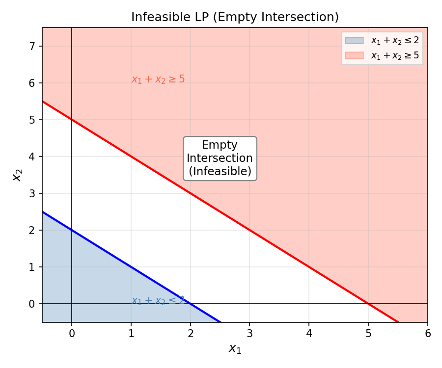
• Infeasible: \(S = \emptyset\). No solution satisfies all constraints.
• Optimal: There exists \(x_0 \in S\) with \(f(x_0) \le f(x)\) for all \(x \in S\). We call \(x_0\) an optimal solution and \(f(x_0)\) the optimal value.
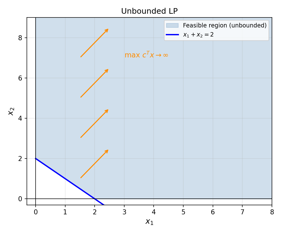
• Unbounded: \(S \ne \emptyset\) but for every \(M \in \mathbb{R}\) there exists \(x \in S\) with \(f(x) < M\). The objective can be made arbitrarily small.
• Feasible but no optimum attained: \(S \ne \emptyset\) and the infimum is finite but not achieved (unusual in LP but possible in NLP).

1.2 Classes of Optimization Problems

1.2.1 Linear Programs

Linear programs are the workhorse of applied optimization: they are rich enough to model most real-world allocation problems, yet tractable enough to solve in polynomial time. Their defining feature — linearity — allows a complete geometric and algebraic theory.

The two forms are interconvertible: introduce slack variables \(x_{n+1}, \ldots\) to turn SIF into SEF; reverse \(\ge\) constraints by multiplying by \(-1\) and split equalities into two inequalities to turn any LP into SIF.

The two standard forms are algebraically equivalent: each can be transformed into the other by introducing slack or surplus variables. Working in SEF simplifies the simplex method’s algebraic description (bases, pivots), while SIF is more natural for duality theory.

Adding integrality constraints makes the problem dramatically harder in general (NP-complete), but for special constraint matrices — such as those arising from network flow and bipartite matching — the LP relaxation automatically produces integer solutions. This is the content of Chapter 5’s results on totally unimodular matrices.

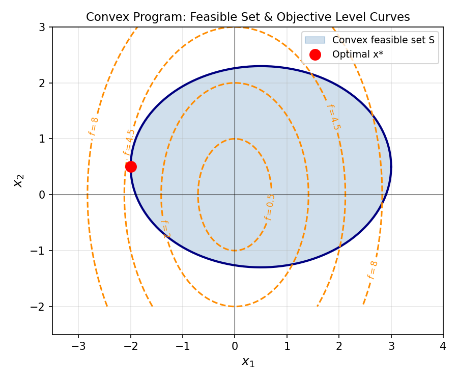
1.2.2 Convex Programs

Convex programs generalize linear programs by allowing curved objective functions and constraints, provided they are all convex. The fundamental insight is that convexity guarantees “no false local minima”: every local minimum of a convex function over a convex set is a global minimum.

Convexity of the feasible set rules out “holes” or disconnected regions — the feasible region is a single connected chunk, which simplifies both analysis and algorithms.

A convex function lies below the chord connecting any two of its points. Geometrically, the “bowl shape” of a convex function ensures that gradient methods always descend toward the global minimum.

Convex programs occupy the “tractable” end of the optimization spectrum: the KKT conditions (Chapter 5) provide necessary and sufficient optimality conditions, and interior-point methods solve them in polynomial time.

1.3 Motivating Examples

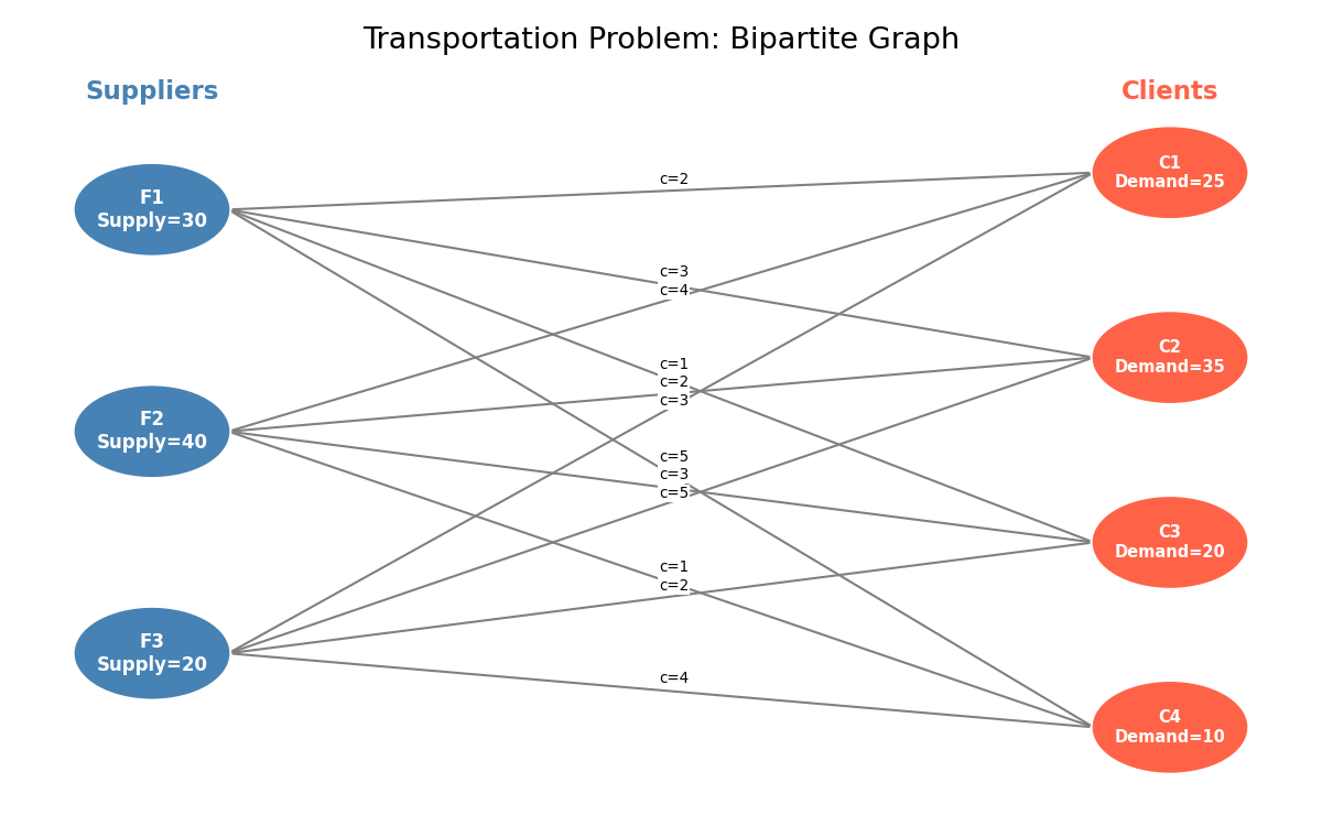
Transportation Problem

A company has a set \(F\) of distribution centers (facilities) and a set \(C\) of clients. Facility \(i\) can supply at most \(u_i\) units; client \(j\) demands exactly \(d_j\) units; the unit cost of shipping from \(i\) to \(j\) is \(c_{ij}\). We seek a minimum-cost shipping plan.

\[\min \sum_{i \in F}\sum_{j \in C} c_{ij} x_{ij}\]

subject to \(\sum_{j \in C} x_{ij} \le u_i\) for all \(i \in F\), \(\sum_{i \in F} x_{ij} = d_j\) for all \(j \in C\), and \(x_{ij} \ge 0\).

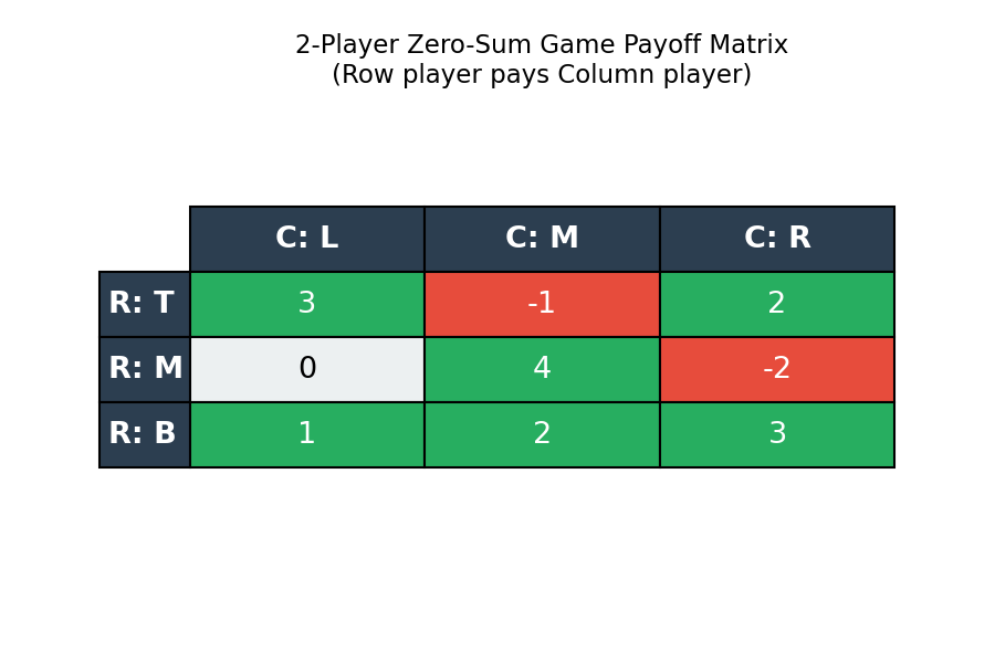
2-Player Zero-Sum Game

\[\max\ v \quad \text{s.t.} \quad \sum_j a_{ij} p_j \ge v\ \forall i,\quad \sum_j p_j = 1,\ p \ge 0.\]

Symmetrically, R’s LP (R-LP) minimizes the maximum expected payout over columns. A remarkable consequence of LP duality is that the optimal values of (C-LP) and (R-LP) are equal — this is the minimax theorem.

Job Assignment and Fair Division

The assignment problem — matching \(n\) workers bijectively to \(n\) jobs at minimum total cost — is an IP. Crucially, its LP relaxation (dropping integrality) automatically has integer extreme points because the constraint matrix is totally unimodular (see Chapter 5).

The fair division problem seeks to distribute items among agents to maximize the Nash welfare \(\prod_i (\sum_j u_{ij} x_{ij})\), equivalently \(\max \sum_i \ln(\sum_j u_{ij} x_{ij})\), a convex program.

---

Chapter 2: Linear Programming Geometry

Chapter 1 introduced LP abstractly. Chapter 2 develops the geometric language — polyhedra, vertices, faces — that makes LP theory visual and intuitive. The key insight is that LP feasible regions are polyhedra, and optimal solutions (when they exist) always occur at vertices. This reduces the infinite optimization problem to a finite combinatorial one.

2.1 Polyhedra and Feasible Regions

The feasible region of an LP is defined by finitely many linear inequalities, each cutting the space with a hyperplane and keeping one side. The intersection of all these half-spaces is a polyhedron.

Polytopes are finite, compact objects — all their “directions” are bounded. The simplex method works especially cleanly on polytopes because the number of vertices is finite, though potentially exponentially large.

The feasible region of any LP is a polyhedron. This geometric fact underpins all of LP theory — algorithms like the simplex method walk along the vertices (extreme points) of this polyhedron.

Extreme points are the “corners” of the polyhedron — the points that cannot be expressed as the midpoint of two other feasible points. These are precisely where optimal solutions live.

Extreme points are “pinned down” by constraints: they cannot wiggle in any direction while staying feasible. The following theorem characterizes them algebraically, connecting the geometric notion to the rank of the tight constraint matrix.

What makes this remarkable is that it bounds the “complexity” of any convex combination: no matter how many points are in \(S\), and no matter how elaborate their convex combinations, you never need more than \(n+1\) of them. In the plane (\(n=2\)), any point in the convex hull of an arbitrary set can be written as a convex combination of just three points — a triangle suffices. In three dimensions, four points (a tetrahedron). This dimensionality bound is tight and beautiful.

The proof is an elegant application of linear independence: if a convex combination uses more than \(n+1\) points, the coefficients satisfy a linear dependence relation (there are too many for \(\mathbb{R}^n\)), which can be used to eliminate one point while maintaining a valid convex combination. Repeating this reduction arrives at \(n+1\) or fewer points.

The following theorem offers an equivalent, and somewhat surprising, characterization of extreme points. It says \(\bar x\) is extreme if and only if removing it from \(S\) does not destroy convexity. Intuitively, a non-extreme point is a “midpoint” of two others — removing it creates a gap in the line segment connecting those two others, breaking convexity. An extreme point, by contrast, is not “needed” as a midpoint by any pair, so removing it leaves convexity intact.

Theorem 2.7.7 below is the algebraic heart of the theory of extreme points. It translates the geometric notion — “cannot be expressed as a midpoint” — into a linear-algebraic rank condition that is checkable by computation.

The corollary gives a useful finiteness bound: since we choose \(n\) linearly independent rows from the \(m\) rows of \(A\) to determine each extreme point, there are at most \(\binom{m}{n}\) extreme points. This bound is exponential, but it is the quantity that controls the worst-case complexity of the simplex method.

A polyhedron with no extreme points must contain an entire line — it extends infinitely in both directions along some direction. The following definition and proposition capture exactly this dichotomy.

Full rank of tight constraints means \(\bar x\) is uniquely determined by those constraints — it is a “vertex” in the algebraic sense. If the rank falls short, a direction exists along which we can move while staying on all tight constraints, so \(\bar x\) lies in the interior of an edge or face.

Two fundamental structural theorems about polytopes follow from the extreme point characterization. The first says a bounded polyhedron is nothing more than the convex hull of its corners; the second says the converse — any finite set of points generates a polytope. Together they close a duality between the “inequality description” and the “vertex description” of polytopes.

What about unbounded polyhedra? A polyhedron that extends to infinity cannot be described purely by its extreme points — it also has extreme rays, directions in which the feasible region extends without bound. The Minkowski sum allows us to decompose any pointed polyhedron into a compact “core” (a polytope spanned by extreme points) and a cone of extreme rays. This decomposition is the key to understanding unbounded LPs: an LP is unbounded precisely when there exists an extreme ray along which the objective improves.

The Minkowski sum gives us a powerful algebraic operation on sets: adding two sets pointwise. Geometrically, \(S + T\) is obtained by “sliding” every copy of \(T\) to every point of \(S\). This operation is exactly what we need to decompose an unbounded polyhedron into its bounded “core” and its cone of unbounded directions.

The next two theorems — together known as the Minkowski-Weyl theorem — provide the complete structural description of polyhedra. Theorem 2.7.14 handles the pointed case, decomposing any pointed polyhedron into a compact part (a polytope) plus a cone of unbounded directions. Theorem 2.7.15 generalizes to all polyhedra, including those containing lines.

Theorem 2.7.15 is the Minkowski-Weyl theorem: every polyhedron can be built by taking a polytope and “extending” it in the directions of a polyhedral cone. This is the complete structural description of polyhedra. When the polyhedral cone is trivial (just the origin), we recover a polytope. When there is no polytope part (the cone is the whole thing), we have a polyhedral cone. The general case is always a sum of these two extreme cases.

Some polyhedra contain entire lines — they extend to infinity in both directions along some vector. Such polyhedra have no extreme points at all. The lineality space captures exactly which directions allow this bidirectional extension.

The two key structural concepts needed to handle polyhedra containing lines are affine subspaces and lineality spaces. An affine subspace is a “shifted” linear subspace — it passes through a specific point but is otherwise flat. The lineality space is the collection of all directions in which the polyhedron extends without bound in both directions simultaneously; it is the “linear part” of the polyhedron.

The culminating structural theorem of this section completes the Minkowski-Weyl decomposition by adding the lineality space. Notice how \(F = P + K + L\) breaks the polyhedron into three orthogonal parts: the bounded core \(P\), the “one-directional” cone \(K\) of extreme rays, and the “two-directional” flat \(L\). This is the most general description of any nonempty polyhedron.

The full decomposition \(F = P + K + L\) is beautiful: every nonempty polyhedron is a “translated” polytope, extended by a cone of rays and a lineality space of lines. From an LP perspective, the lineality space contains directions that never affect objective value — they are the “neutral” directions. The cone contains directions that may improve the objective (unboundedness), and the polytope contains the bounded part where optimal vertices live.

Theorems 2.7.20 and 2.7.21 are the “vertex description” counterparts to the “halfspace description” of polytopes and cones. They say that the two perspectives — describing a set by the halfspaces that contain it (the \(H\)-representation) or by the vertices and rays that generate it (the \(V\)-representation) — are equivalent. Every polytope can be built as the convex hull of finitely many points, and every polyhedral cone can be built as the conic hull of finitely many rays. Converting between these representations is a fundamental computational problem in LP.

This theorem says that a polytope is completely described by its vertices — a finite set of points. Every other feasible point is a convex combination of vertices. This is both a structural fact and the basis for LP optimality theory.

The proof is a “greedy tightening” argument: start at any optimal point, and if it is not a vertex, slide along the constant-objective face until a new constraint becomes tight. Repeat until full rank — an extreme point — is reached. This justifies the simplex method’s vertex-walking strategy: we need only search among vertices.

2.2 Feasibility: Fourier-Motzkin and Farkas

Having characterized optimal solutions geometrically (vertices of polyhedra), we now address the prior question: is the system \(Ax \le b\) feasible at all? Fourier-Motzkin elimination gives a constructive procedure, and Farkas’ lemma extracts from it a clean algebraic certificate of infeasibility.

\[\frac{1}{a_{ln}}\left(b_l - \sum_{j=1}^{n-1} a_{lj}x_j\right) \le \frac{1}{a_{kn}}\left(b_k - \sum_{j=1}^{n-1} a_{kj}x_j\right).\]

The new system in \(n-1\) variables is feasible if and only if the original is. Repeating until no variables remain: the final system is a set of scalar inequalities \(0 \le \gamma_i\); feasibility holds iff all \(\gamma_i \ge 0\). If infeasible, FME produces a certificate \(u \ge 0\) with \(u^T A = 0\) and \(u^T b < 0\), which is exactly the content of Farkas’ Lemma.

Farkas’ lemma is one of the most important results in LP theory. It says feasibility and infeasibility have “certificates” — proofs that can be verified in polynomial time. The great philosophical point is this: if you claim a system is infeasible, how do you convince someone else? You need to exhibit a short proof — a Farkas certificate. The lemma says such a certificate always exists.

There are three variants of Farkas’ lemma, each suited to a different LP form. They all say the same thing in different algebraic disguises: feasibility and infeasibility are dual to each other, and exactly one holds. Understanding which variant applies to which situation is a core skill in LP.

The first variant handles the purest case: linear equations with no sign restrictions on \(x\).

The key insight here is that alternative (II) is exactly a certificate of linear dependence: \(y\) shows that \(b\) is not in the column span of \(A\). This is precisely the familiar statement from linear algebra about the column space.

The second variant handles inequality systems — the most common form in LP. Notice how the non-negativity of \(u\) in alternative (II) corresponds to the requirement that the “combination” of constraints uses the inequalities in their stated direction.

Notice how the non-negativity \(u \ge 0\) in alternative (II) corresponds to the fact that the certificate combines the inequalities of (I) in their stated direction — you may scale each inequality by a non-negative factor but not flip it. If you could flip inequalities, you could manufacture contradictions out of thin air; the sign constraint on \(u\) prevents this.

The third variant is the most directly useful for LP: it handles inequality systems with non-negative variables, matching the Standard Inequality Form of LP. What makes this remarkable is that the certificate \(y\) in alternative (II) provides an explicit linear combination of the constraints that “derives” a contradiction — it witnesses infeasibility with arithmetic you can check by hand.

The proof shows mutual exclusivity by a “dot product sandwich” argument: if (I) holds, then any \(y\) satisfying the constraints in (II) would give \(0 > b^T y \geq 0\), a contradiction. The existence of (II) when (I) fails follows from FME.

Geometric interpretation: \(b\) lies in the cone \(\text{cone}\{A_1, \ldots, A_n\}\) if and only if no hyperplane \(\{y : y^T \delta = 0\}\) separates \(b\) from the cone. Farkas’ Lemma says either \(b\) is in the cone (I), or a separating hyperplane exists (II). This is the “alternative theorem” of linear algebra: exactly one of the two alternatives holds.

---

Chapter 3: The Simplex Method

Chapter 2 established the geometry: LP optimal solutions occur at vertices of polyhedra. Chapter 3 develops the algebra and algorithms that exploit this structure. The simplex method walks along edges from vertex to vertex, improving the objective at each step. But before the algorithm, we need the dual LP — the “other side” of the problem that provides optimality certificates.

3.1 LP Duality: Motivation

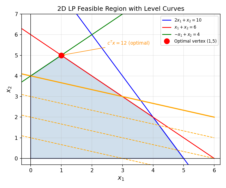
How can we certify the optimality of a feasible solution? By taking nonnegative linear combinations of the constraints. For the LP \(\max\ 2x_1 + x_2\) subject to \(x_1 - 2x_2 \le 4,\ -x_1 + x_2 \le 10,\ \ldots\), a particular nonnegative combination of constraints yields \(2x_1 + x_2 \le 10\). Since the objective equals 10 at the feasible point \((0, 10)\), this proves optimality.

This motivates a systematic “dual” LP whose feasible solutions provide upper bounds on the primal objective.

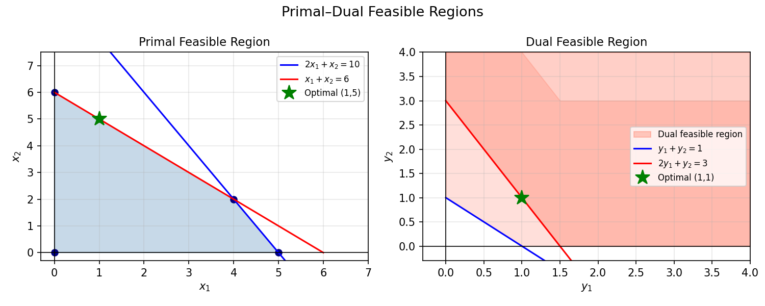
The dual LP is constructed by associating one variable \(y_i\) with each primal constraint. Multiplying the \(i\)-th constraint by \(y_i \geq 0\) and summing gives an upper bound on the primal objective — and minimizing this upper bound over all such \(y\) is the dual problem.

The dual is another LP. Its feasible solutions certify upper bounds on the primal: if \(b^T y = 17\) for some feasible dual \(y\), then the primal optimum is at most 17. Strong duality says the best (smallest) such certificate exactly matches the primal optimum.

3.2 Weak and Strong Duality

Weak duality is the trivial direction: any feasible dual solution provides an upper bound on the primal.

Weak duality says the primal and dual objectives form a “sandwich”: any primal feasible objective value is at most any dual feasible objective value. But it leaves open the question: how large is the gap? Could the primal optimum be strictly below the dual optimum? Strong duality — one of the most powerful results in all of optimization — says the answer is no. Under feasibility of both sides, the gap is exactly zero.

Notice the elegance of what this achieves. The primal problem asks “how good can we do?” The dual asks “how tight can we certify a bound?” Strong duality says these two processes converge to the same answer. The algorithm (simplex, interior point) and the certificate (dual solution) agree.

What was just shown is that strong duality is not a coincidence — it is Farkas’ lemma applied one level up, to the combined optimality system. The proof technique is characteristic of LP theory: assume the gap is positive, derive a Farkas certificate, observe the certificate contradicts something already known, conclude no gap exists. This pattern repeats throughout the theory.

Notice what Lemma 2.3.6 says geometrically: dual infeasibility means no nonneg combination of constraints pins down the objective, so there is an unbounded ray in the primal feasible region along which the objective grows without limit. The Farkas certificate \(d\) is literally this unbounded direction.

This “trichotomy” is the complete classification of LP outcomes. The four-way classification from Chapter 1 reduces to three: the “feasible but no optimum attained” case cannot occur for LPs because the feasible region is a closed polyhedron (compact level sets). The interplay between primal and dual gives a 3×3 grid of possible outcomes for the pair \((P), (D)\), and remarkably only four entries in that grid can actually occur: both optimal, \((P)\) unbounded / \((D)\) infeasible, \((P)\) infeasible / \((D)\) unbounded, and both infeasible. This is a complete characterization.

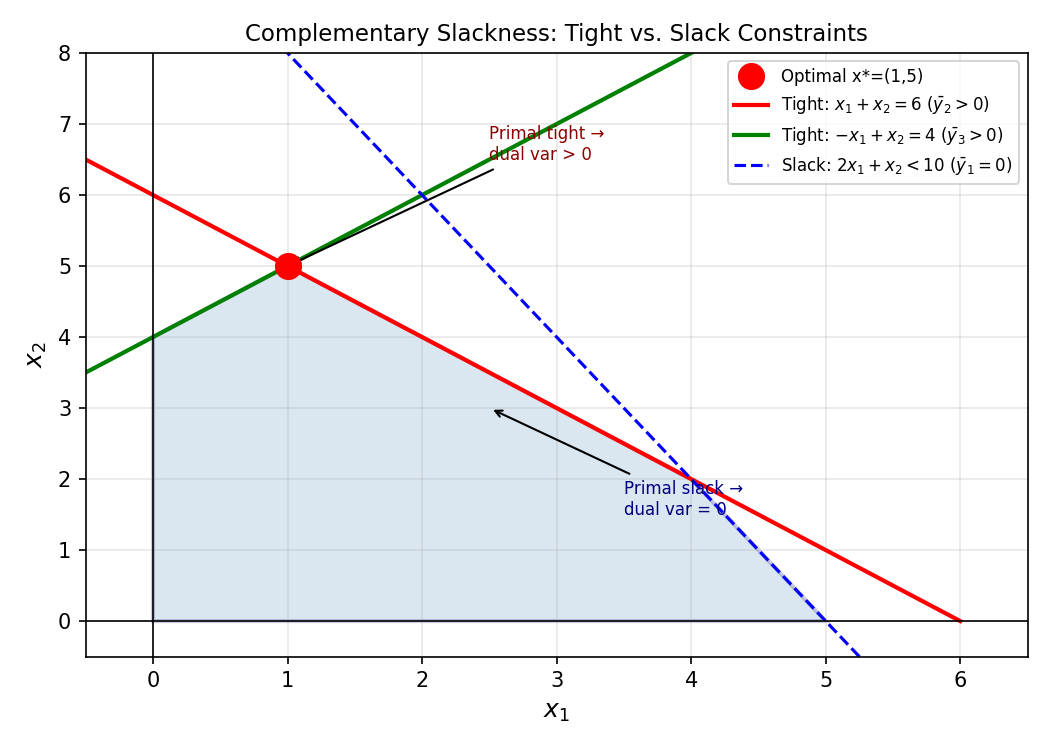
3.3 Complementary Slackness

Strong duality tells us that at optimality, the primal and dual objective values are equal. But “the two objectives are equal” is a global condition — it is hard to check without already knowing both optima. Complementary slackness translates this global equality into a system of local “on/off” conditions on individual variables and constraints. The key insight is that the equality \(c^T \bar x = b^T \bar y\) forces each term in a sum of nonnegative quantities to be exactly zero, giving sharp pointwise conditions.

In practice, complementary slackness is used in two ways. First, given a candidate pair \((\bar x, \bar y)\), one can verify optimality by checking the CS conditions — no need to solve the LP again. Second, one can use the CS conditions to find the optimal dual given a primal solution, or vice versa: fix one solution, enforce CS conditions, and solve for the other.

Complementary slackness (CS) translates the condition \(c^T \bar x = b^T \bar y\) into a system of “on/off” conditions on the variables and constraints.

The proof extracts CS from the “sandwich” equality in weak duality: the sum of nonneg terms equals zero, so every term must be zero individually. This “each term is zero” condition is exactly the complementary slackness. In practice, CS conditions allow us to verify optimality of a claimed solution by checking a list of “either-or” conditions — each variable is either zero, or its corresponding dual constraint is tight.

The definitions of valid inequalities, cones, and active constraints are the vocabulary of duality geometry. A valid inequality is any constraint that every feasible point satisfies; dual variables generate valid inequalities by taking nonneg combinations of the primal constraints. Active constraints are the ones “touching” the current point — the boundary the point rests against. These concepts connect the algebra of CS conditions to the geometry of extreme points.

Proposition 2.5.6 below is the geometric heart of LP optimality. It says a feasible point is optimal precisely when the objective direction \(c\) lies in the cone generated by the active constraint normals. Intuitively: if you stand at a corner of the feasible region and the “uphill” direction of the objective is blocked by the walls you are touching, you are at the optimum. If the objective points “outside” the cone of active walls, you can move along the boundary and improve.

Proposition 2.5.8 shows that strong duality subsumes Farkas’ lemma — the two results are not independent but are part of the same duality fabric. Farkas is “strong duality for the trivial LP.”

Physical interpretation: Think of each hyperplane \(a_i^T x = b_i\) as a wall in the feasible region. The objective \(c\) acts like a force on a particle. The particle reaches equilibrium (optimality) when \(c\) is balanced by normal forces from the walls it touches (tight constraints), with the normal force magnitudes being the dual variables. Walls not touching the particle exert no force, so their dual variables are zero.

3.4 Duality Table and Shadow Prices

The strong duality theorem and CS conditions extend beyond the standard SIF formulation to general LP forms. The duality table below is a mechanical rule for constructing the dual from any LP: match each primal constraint type to a dual variable type, and vice versa. This table should be memorized — it is the “grammar” of LP duality.

For general LPs the primal-dual correspondence is:

Primal (max)	Dual (min)
\(\le\) constraint	\(\ge 0\) variable
\(\ge\) constraint	\(\le 0\) variable
\(=\) constraint	free variable
\(\ge 0\) variable	\(\ge\) constraint
\(\le 0\) variable	\(\le\) constraint
free variable	\(=\) constraint

Economic interpretation: In the resource-allocation LP \(\max c^T x\) s.t. \(Ax \le b,\ x \ge 0\), where \(b_i\) is the supply of resource \(i\), the optimal dual variable \(\bar y_i\) is the shadow price — the rate of change of the optimal value with respect to an increase in \(b_i\). This follows directly from strong duality: if \(b_i \to b_i + \varepsilon\), the optimal value changes by approximately \(\varepsilon \bar y_i\).

LP equivalence is important because the simplex method, duality theory, and Farkas’ lemma are each stated for specific standard forms. Equivalence ensures that all these tools apply regardless of how the LP is originally written. Two LPs are equivalent not just when they have the same feasible region, but when certificates of optimality, infeasibility, and unboundedness translate efficiently between them.

The following strong duality theorem for general LPs is the culmination of all the duality theory developed so far. It applies to any LP, regardless of whether variables are free or sign-constrained, and regardless of whether constraints are equalities or inequalities. The proof reduces to the SIF case using equivalence transformations.

3.5 Geometry of Duality

The algebraic optimality conditions have a beautiful geometric interpretation. A feasible point is optimal if and only if the objective vector is “trapped” by the normals of the active constraints — it cannot point in any direction that would increase the objective while staying feasible.

Valid inequalities are constraints that every feasible point satisfies — they can be added to the LP formulation without changing the feasible region. They are also the “witnesses” in duality: a dual feasible \(y\) produces a valid inequality \(c^T x \le b^T y\) for the primal.

This says: \(\bar x\) is optimal precisely when the objective direction \(c\) lies in the cone generated by the active constraint normals — exactly the equilibrium condition described physically above. If \(c\) pointed outside this cone, we could move in the direction of \(c\) while staying feasible (by moving away from the active constraints), increasing the objective — contradicting optimality.

---

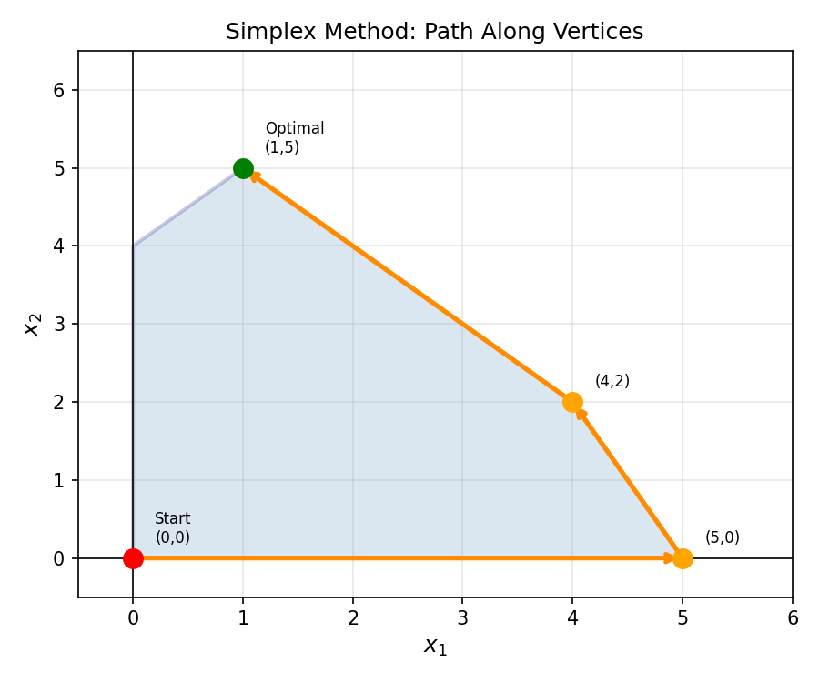
Chapter 4: The Simplex Method

Chapter 3 developed LP duality and optimality conditions. Chapter 4 turns these conditions into a concrete algorithm. The simplex method is a vertex-walking algorithm for LPs in Standard Equality Form (SEF). It exploits the theorem that an optimal solution, if it exists, can always be found at a vertex (extreme point) of the feasible polyhedron. Each pivot moves from one vertex to an adjacent one with a strictly better objective value — a finite process that must terminate at an optimum.

4.1 Bases and Basic Feasible Solutions

Work with \((P): \max\ c^T x,\ Ax = b,\ x \ge 0\) where \(A \in \mathbb{R}^{m \times n}\), \(\operatorname{rank}(A) = m\).

The algebraic notion of a basis corresponds to the geometric notion of a vertex: each vertex of the polyhedron is determined by exactly \(m\) linearly independent tight constraints. To turn this geometric insight into an algorithm, we need an algebraic handle on vertices — that is what bases and basic feasible solutions provide.

Think of it this way. We have \(n\) variables and \(m\) equality constraints. The equality constraints form an underdetermined system: there are infinitely many solutions. A basis \(B\) of size \(m\) picks out \(m\) “special” variables (the basic variables) and forces all other variables to zero. The resulting unique solution \(x_B = A_B^{-1} b,\ x_N = 0\) is the basic solution. If it happens to be non-negative, it is a basic feasible solution — and this corresponds exactly to a vertex of the feasible polytope.

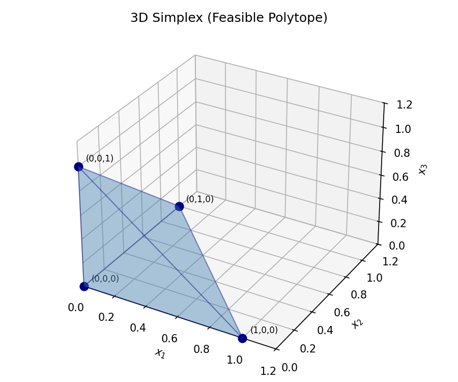
The word “simplex” in the simplex method comes from the following geometric object — in low dimensions, the simplest possible polytope with the most basic structure.

A BFS corresponds to a vertex of the feasible polyhedron: the non-basic variables at zero are the “tight constraints” \(x_j = 0\), and together with \(Ax = b\) they pin down the vertex uniquely.

The equivalence between BFS, linear independence, and extreme points is the cornerstone of the simplex method’s correctness:

This three-way equivalence confirms that the simplex method — which moves between BFS — is indeed walking along the vertices of the feasible polytope. The algebraic pivot corresponds precisely to the geometric step from one vertex to an adjacent one.

4.2 Simplex Algorithm: Pivot Steps

Each simplex pivot moves from the current BFS to a better adjacent one. The key insight is that each step decomposes the problem into: (a) which non-basic variable to “bring in” (the entering variable), and (b) which basic variable to “kick out” (the leaving variable). The entering variable is chosen to improve the objective (positive reduced cost); the leaving variable is determined by the ratio test, which ensures we do not violate feasibility by overshooting.

The reduced costs \(\bar c_N = c_N - A_N^T \bar y\) are the true “value” of increasing each non-basic variable, accounting for the indirect effect through the basic variables. A positive reduced cost means increasing that variable strictly improves the objective — it is “under-priced” relative to its shadow price. When all reduced costs are non-positive, no non-basic variable is worth increasing, and the current BFS is optimal.

The ratio test in step 7 deserves special attention. When we increase the entering variable \(x_k\) from zero, the basic variables change as \(x_B \leftarrow x_B - d x_k\). The minimum ratio \(\bar\alpha = \min\{x_j/d_j : d_j > 0\}\) tells us how much we can increase \(x_k\) before some basic variable hits zero (and must leave the basis). This is exactly the constraint that keeps all variables non-negative.

Given a feasible basis \(B\) and corresponding BFS \(\bar x\):

1. Compute the dual variable \(\bar y = A_B^{-T} c_B\) (solution to \(A_B^T y = c_B\)).
2. Compute reduced costs \(\bar c_N = c_N - A_N^T \bar y\).
3. If \(\bar c_N \le 0\): stop — \(\bar x\) is optimal (and \(\bar y\) is dual optimal).
4. Pick any entering variable \(k \in N\) with \(\bar c_k > 0\) (improving direction).
5. Compute pivot direction \(d = A_B^{-1} A_k\).
6. If \(d \le 0\): stop — \((P)\) is unbounded.
7. Compute step size \(\bar\alpha = \min\{x_j / d_j : j \in B,\ d_j > 0\}\) and leaving variable \(l\) achieving the minimum (ratio test).
8. Update basis: \(B' = B \cup \{k\} \setminus \{l\}\) and \(\bar x' = \bar x + \bar\alpha \bar d\).

\[c^T x = c_B^T A_B^{-1} b + \sum_{j \in N} \bar c_j x_j.\]

The constant term is the current value. Since \(\bar c_k > 0\) and we increase \(x_k\), the objective strictly increases (when \(\bar\alpha > 0\)).

4.3 Termination and Degeneracy

The simplex method must terminate because there are only finitely many bases. But degeneracy — where multiple bases correspond to the same BFS — can cause the algorithm to cycle indefinitely without making progress.

The next two propositions confirm that each step of the simplex method maintains the invariants that make it work: after a pivot, the new solution is still a BFS (Proposition 2.8.2), and when no pivot can improve the objective, the current solution is optimal (Proposition 2.8.3). Together they establish the correctness of the algorithm.

Proposition 2.8.3 is the “certificate of optimality” half of the simplex method: when the algorithm halts with \(\bar c_N \le 0\), the dual solution \(\bar y\) computed in step 1 is dual feasible, and by construction the primal-dual pair \((\bar x, \bar y)\) satisfies complementary slackness. Strong duality then confirms they are both optimal. The simplex method does not merely find a solution — it simultaneously finds a proof of optimality.

When \(\bar\alpha > 0\), every pivot strictly improves the objective, so no basis can be revisited. The bound \(\binom{n}{m}\) is the number of possible bases — an exponential bound, but one that is rarely approached in practice.

Degeneracy occurs when more than \(m\) constraints are tight at a vertex — the vertex is an intersection of “too many” hyperplanes. Geometrically, degenerate vertices look like regular vertices but may cause the algorithm to walk in circles through different bases all representing the same vertex.

Bland’s Rule: Choose the entering variable \(k\) and leaving variable \(l\) both with the smallest index among all eligible candidates. This guarantees termination.

Bland’s rule breaks the symmetry that causes cycling: by imposing a total order on variable choices, it ensures the algorithm always makes a definite “progress” signal even when the objective does not improve.

4.4 Lexicographic Simplex and Two-Phase Method

The degeneracy problem — stalling at a degenerate vertex — and the initialization problem — finding an initial BFS — are the two practical obstacles to running the simplex method on a real LP. The lexicographic pivot rule addresses the former; the two-phase method addresses the latter.

An elegant alternative to Bland’s rule is perturbation: slightly modify the right-hand side \(b\) to eliminate all degeneracy. The perturbed LP has no degenerate vertices, so the simplex method terminates by the basic finite termination theorem.

To handle degeneracy more elegantly, perturb \(b\) to \(b + \sum_{i=1}^m \varepsilon^i e_i\) with \(1 \gg \varepsilon_1 \gg \cdots \gg \varepsilon_m > 0\). The lexicographic simplex compares ratio-test candidates lexicographically, breaking all ties. The perturbed LP is automatically nondegenerate, guaranteeing strict improvement at every step.

The initialization problem is the other practical challenge: the simplex method requires a starting BFS, but none may be obvious from the LP’s original formulation. The two-phase method is a beautiful resolution: solve a modified LP (Phase I) whose optimal value tells us whether the original LP is feasible, and whose optimal solution gives us the starting BFS for Phase II. The auxiliary LP always has an obvious starting BFS — the artificial variables \(s_i\) are set to \(b_i\) (assuming \(b \ge 0\) after possibly flipping rows).

\[\text{(P-AUX):}\ \max\ -\mathbf{1}^T s \quad \text{s.t.}\ Ax + Is = b,\ x,s \ge 0.\]

The basis \(B = \{n+1,\ldots,n+m\}\) gives an immediate BFS with \(s = b \ge 0\). If the optimal value of (P-AUX) is zero, then a feasible basis for (P) has been found; otherwise (P) is infeasible.

The simplex method not only finds a primal optimal solution \(\bar x\) — it simultaneously computes a dual optimal solution \(\bar y = A_B^{-T} c_B\). At termination, the pair \((\bar x, \bar y)\) satisfies complementary slackness. The abridged CS theorem below gives a stronger form of this: not only is one side of each CS pair zero, but their sum is strictly positive. This “complementary” relationship is exact — no partial zeroes are possible.

This is a strengthening of ordinary CS: not only does one of the two quantities vanish, but their sum is strictly positive — so exactly one is zero and the other is strictly positive.

---

Chapter 5: Applications and Special Structure

With the theory and algorithm of LP developed, Chapter 5 turns to applications: combinatorial optimization (matchings, flows, games), special matrix structure (totally unimodular matrices), and extensions to nonlinear optimization (convex programs, KKT conditions). The common thread is that linear programming, when applied to problems with special structure, yields much more than just a solution — it yields structural insight, integer optima automatically, and a bridge to combinatorial min-max theorems.

5.1 LP Unboundedness and Infeasibility (Geometric)

An LP can fail in two ways. Geometrically:

• Infeasible: the constraint halfspaces have empty intersection.
• Unbounded: the feasible region extends infinitely in the direction of improving objective.

5.2 Combinatorial Optimization and Integer Programs

Many optimization problems arising from combinatorics — who matches to whom, which path is shortest, how much flow fits through a network — are naturally formulated as integer programs. The key insight is that for many such problems, the LP relaxation (dropping integrality) automatically produces integer solutions, making them solvable in polynomial time despite their integer formulation.

Many combinatorial problems (matching, shortest path, max-flow) are naturally formulated as integer programs. The LP relaxation drops the integrality constraint:

\[(\text{IP})\ \max c^T x,\ Ax \le b,\ x \in \mathbb{Z}^n \quad \le \quad (\text{LP})\ \max c^T x,\ Ax \le b.\]

The LP optimal value is an upper bound on the IP optimal value. Equality holds when the LP solution is automatically integral — a situation governed by totally unimodular matrices.

The integer hull captures all integer points that can be convexly combined — it is the “best LP relaxation” of the integer program.

The integer hull is the most important polyhedral object in integer programming. It is the convex hull of all integer feasible points — the “LP relaxation of the LP relaxation” that is tight for integer solutions. If we knew the integer hull explicitly (as a set of linear inequalities), we could solve any IP over these constraints as an LP. The challenge of IP is precisely that the integer hull may require exponentially many inequalities to describe. Theorems 3.2.1 and 3.2.2 confirm that the integer hull is always a polyhedron — it is a well-structured object, even if its description is complex.

When \(P = P_I\), the LP and the IP have the same optimal value for every objective — the LP is an “exact” relaxation. This is the ideal situation, and it holds whenever \(A\) is totally unimodular.

Theorem 3.2.4 collects five equivalent characterizations of the condition \(P = P_I\). This five-way equivalence is remarkable: it shows that the condition “the LP relaxation always has an integral optimal solution” is equivalent to “every extreme point is integral” (a structural condition), “the LP optimal is always integral” (an objective-value condition), and even “the dual LP optimal is always integral” (a condition on the dual). Each equivalence opens a different avenue for proving or refuting \(P = P_I\). In practice, the most useful direction is (1) \(\Rightarrow\) (3): if we can verify that every extreme point of \(P\) is integral (e.g., by showing \(A\) is TU), then we conclude the LP always has an integral optimal solution.

5.3 Totally Unimodular Matrices

The condition that makes LP relaxations automatically integral is total unimodularity — a condition on the constraint matrix \(A\) that ensures all bases have determinant \(\pm 1\), forcing Cramer’s rule to produce integers.

Total unimodularity is a strong algebraic condition: not just the full matrix, but every square submatrix must have determinant in \(\{-1, 0, 1\}\). Yet many natural constraint matrices from combinatorics satisfy it.

Theorem 3.3.3 establishes that total unimodularity is equivalent to two other properties: determinant \(\pm 1\) for every basis, and integer-valued inverse for every basis. The equivalence (1) \(\Leftrightarrow\) (3) is immediate from Cramer’s rule: if \(\det A_B = \pm 1\), then \(A_B^{-1} = \frac{\text{adj}(A_B)}{\det A_B}\) has integer entries. The equivalence (2) \(\Leftrightarrow\) (3) is the crucial LP statement: integer right-hand sides and integer inverse bases produce integer extreme points.

Proposition 3.3.4 lists the closure properties of TU matrices — operations that preserve total unimodularity. These are extremely useful in practice: they tell us that we can augment a TU matrix with an identity block, take its transpose, or scale its rows by \(\pm 1\), and the result is still TU. This allows us to recognize TU structure even when it is disguised by routine LP transformations such as adding slack variables or switching to SEF.

Theorems 3.3.5 and 3.3.6 are the payoff of TU for LP in practice. They say that if \(A\) is TU and \(b\) is integral, then the LP over \(\{Ax \le b\}\) or \(\{Ax \le b, x \ge 0\}\) automatically has integral extreme points — no matter what the objective is. This means: solve the LP (ignoring integrality), and the optimal solution you get is already integral. No branch-and-bound, no cutting planes, no extra work.

Now the critical question is: which matrices actually arise in practice are TU? The two most important examples come from graphs. Theorem 3.3.7 says the node-arc incidence matrix of any directed graph is TU — this single fact implies that network flow problems (shortest path, maximum flow, minimum cost flow) all have integral LP relaxations. The corollary then gives us the bipartite case, which drives the matching theory.

The proof is a simple application of Cramer’s rule: inverse of an integer matrix with determinant \(\pm 1\) is another integer matrix. TU makes every basis inversion produce an integer result, so every extreme point is integral.

Key examples of TU matrices:

1. The node-arc incidence matrix of any directed graph is TU. Each column (arc) has exactly one \(+1\) (head) and one \(-1\) (tail), so any square submatrix has determinant in \(\{-1, 0, 1\}\) (by induction on size).

2. The incidence matrix of any bipartite graph is TU. Proof: orient all edges from one side of the bipartition to the other to get a directed graph; its incidence matrix is TU by (1), and the undirected incidence matrix differs only by row signs.

These facts are tight: the incidence matrix of an odd cycle (non-bipartite graph) is not TU. The determinant of the incidence matrix of a triangle is \(\pm 2\), violating TU. This is why bipartiteness is necessary for König’s theorem: non-bipartite graphs have incidence matrices that are not TU, so their LP relaxations may have fractional optima.

5.4 König’s Theorem

König’s theorem — first proved in 1916 by purely combinatorial means — follows from total unimodularity as an almost immediate corollary. The LP lens makes the underlying structure transparent. What makes this theorem striking is that it asserts the equality of two quantities that are trivially in a one-sided relationship: a matching and a vertex cover cannot have the same size unless both are optimal. König says they always can be made equal in bipartite graphs — a min-max equality that has no analog in general graphs.

The key insight here is that maximum matching is a primal LP (maximize the number of edges selected, subject to each vertex being covered at most once), and minimum vertex cover is its dual (minimize the number of vertices selected, subject to each edge being covered by at least one selected vertex). Strong LP duality gives equal objective values; TU of the bipartite incidence matrix gives integral solutions. These two facts together prove König in two lines.

The proof is beautifully concise: the two facts (TU gives integrality; LP duality gives equal optima) combine to prove a non-trivial combinatorial equality in two lines. This is the power of the LP/TU framework: combinatorial theorems become consequences of algebraic structure.

Theorem 3.8.1 is a clean dichotomy theorem for perfect matchings in balanced bipartite graphs: either the graph has a perfect matching, or it has a “deficient set” — a subset of one side that is too small in the neighborhood to be matched. This is the contrapositively stated form of Hall’s theorem, and it gives an explicit obstruction certificate whenever a perfect matching does not exist.

5.5 Maximum Flow — Minimum Cut

The Max-Flow Min-Cut theorem admits a proof identical in structure to König’s, once we observe that the flow LP has a TU constraint matrix. This unifies two seemingly different theorems under the same algebraic roof. Notice how the “LP + TU” framework becomes a proof machine: once you identify the right LP formulation and verify TU of the constraint matrix, you get (a) an integral optimal solution automatically, and (b) via LP duality, a min-max equality theorem. The Max-Flow Min-Cut theorem, König’s theorem, and Hall’s theorem are all instances of this same machine applied to different combinatorial structures.

The proof is identical in structure to König’s: the flow LP has a TU constraint matrix (the node-arc incidence matrix of the directed graph), so the LP and its dual both have integral optima; the dual LP encodes the minimum cut problem. The integrality of the maximum flow is a free consequence — it follows from TU rather than from the Ford-Fulkerson algorithm.

The polyhedral theory underlying these results relies on the notions of dimension, faces, and facets. These concepts give us a “stratification” of a polyhedron: extreme points (dimension 0), edges (dimension 1), two-dimensional faces, and so on up to facets (dimension \(n-1\)). This hierarchy is not just combinatorially interesting — it has direct algorithmic implications. Facets are the “essential” inequalities in any LP formulation: Theorem 3.6.1 says every minimal description of a full-dimensional polyhedron has exactly one inequality per facet. Knowing the facets of the integer hull \(P_I\) would give the tightest possible LP relaxation.

Facets of \(P_I\) give the strongest valid inequalities for the integer hull and help judge IP formulations.

The following theorems are “integer analogs” of Farkas’ lemma — alternative theorems in the setting of integer solutions rather than real solutions. They answer the question: when does the system \(Ax = b\) have an integer solution? Just as Farkas’ lemma characterizes real feasibility via a dual certificate, these results characterize integer feasibility via rational certificates involving the integrality of \(A^T y\) and \(b^T y\). Notice how each steps up in generality: from rational systems over \(\mathbb{Q}\), to real systems with approximate integer solutions.

Kronecker’s Approximation Theorem is a beautiful analytic result: for real (possibly irrational) systems, exact integer solutions may not exist, but the question is whether arbitrarily close approximations can be found. The alternative is again a certificate — a dual vector \(y\) that “distinguishes” the integer lattice from the target \(b\). This is the bridge between number theory and LP that makes the theory of integer programming so deep.

The Hermite Normal Form is the integer analog of row reduction. Just as every matrix over a field can be reduced to row echelon form by elementary row operations (which correspond to unimodular transformations over \(\mathbb{Z}\)), every integer matrix can be reduced to Hermite Normal Form by unimodular column operations. This provides a canonical form for integer linear algebra, useful for solving integer systems and analyzing the lattice structure underlying IP.

5.6 Hall’s Theorem and Weighted Matching

Hall’s theorem gives the existential condition for perfect matchings in bipartite graphs. The LP/duality perspective gives an algorithmic extension: the Hungarian algorithm for maximum weight perfect matching iteratively updates the dual to expand the “equality subgraph” until it admits a perfect matching.

Hall’s theorem is the classical existential statement. The LP approach upgrades it to an algorithm: by maintaining dual feasibility and expanding the equality subgraph, we find a maximum weight perfect matching rather than merely certifying existence.

\[\bar y_v' = \begin{cases} \bar y_v - \varepsilon & v \in S \\ \bar y_v + \varepsilon & v \in N_{G(\bar y)}(S) \\ \bar y_v & \text{otherwise} \end{cases}\]

where \(\varepsilon = \min\{\bar y_u + \bar y_v - c_{uv} : uv \in E,\ u \in S,\ v \notin N_{G(\bar y)}(S)\}\). Each iteration decreases the dual objective by an integer amount \(|S| - |N_{G(\bar y)}(S)| \ge 1\), guaranteeing termination.

5.7 Nonlinear and Convex Optimization

The final section steps beyond LP to the broader world of nonlinear optimization. The key results parallel the LP theory: there are first-order optimality conditions (analogous to LP’s CS conditions), second-order tests (via the Hessian), and gradient methods (analogous to the simplex method). For convex programs, these conditions are both necessary and sufficient.

In nonlinear optimization, the feasible set and/or objective can be arbitrary (smooth) functions. Convex programs occupy the “easy” end of this spectrum.

Before developing the theory of convex optimization, we need to recall the topological foundation. The key concepts — interior, closure, compactness — serve as the “stage” on which convex analysis plays out. These are not abstract formalities; they directly govern when optimizers exist and when gradient conditions are meaningful.

Compactness is the magic condition that guarantees optima exist. Without it, a continuous function on a closed set might not attain its minimum (it approaches the infimum asymptotically). The Bolzano-Weierstrass theorem is the key lemma: every sequence in a compact set has a convergent subsequence that stays in the set.

The Weierstrass theorem is the fundamental existence result for optimization: any continuous function on a compact set attains its minimum and maximum. This is why “compact feasible region + continuous objective” is the gold standard for an optimization problem that is well-posed. In LP theory, polytopes are compact, and continuous (linear) objectives always attain their optimum — which is the LP “no infimum without minimum” property.

For unbounded feasible regions (closed but not compact), compactness fails and Weierstrass does not directly apply. Coercivity is the replacement condition: a coercive function “blows up” as we walk to infinity, so we can always restrict attention to a bounded sublevel set without loss of generality. This converts the unbounded problem to a compact one, recovering the Weierstrass guarantee.

The epigraph is a powerful conceptual device: it “lifts” a function into a set in one higher dimension, converting questions about functions into questions about convex sets. The graph of \(f\) is the boundary of its epigraph; the epigraph is everything “above” the graph. This geometric perspective unifies many convexity arguments, since tools from convex geometry (like separation theorems) can be applied directly to the epigraph.

Theorem 4.2.3 gives the gradient characterization of convexity. It says convex functions lie above their first-order Taylor expansions: the tangent hyperplane at any point is a global lower bound. This is the “supporting hyperplane property” for graphs of functions. For optimization purposes, it means that a local condition (the gradient at one point) gives global information — if \(\nabla f(\bar x) = 0\) and \(f\) is convex, then \(\bar x\) is a global minimizer.

Theorem 4.2.9 gives the monotone gradient characterization: a differentiable function is convex if and only if its gradient is monotone (in the sense that the gradient “points more” in the direction of increasing function values). This condition is useful for verifying convexity of functions where the Hessian is difficult to compute, and it is also the key condition that guarantees gradient descent methods converge.

The first-order optimality condition says the gradient at \(\bar x\) must point “outward” relative to \(S\): moving to any other feasible point would not decrease the objective. For unconstrained minimization (\(S = \mathbb{R}^n\)), this reduces to \(\nabla f(\bar x) = 0\).

The Hessian characterization gives a practical test for convexity: check that all eigenvalues of \(H_f(x)\) are non-negative at every point. Positive semidefiniteness means the function “curves upward” in every direction — the bowl shape that defines convexity.

Gradient methods iteratively update \(\bar x \leftarrow \bar x + \alpha d\):

• Steepest descent: \(d = -\nabla f(\bar x)\). Simple but slow (linear convergence).
• Newton’s method: \(d = -[H_f(\bar x)]^{-1} \nabla f(\bar x)\). Quadratic convergence near the optimum but requires computing and inverting the Hessian.

The Separating Hyperplane Theorem is the geometric backbone of all of duality theory — it says that convexity is the condition under which “you cannot be confused about which side you are on.” If a point is outside a convex set, there is always a hyperplane that cleanly separates them. This result was used implicitly throughout the LP theory (in the geometric proof of Farkas’ lemma, and in the cone optimality condition), and now it becomes explicit.

A supporting hyperplane is a “touching” hyperplane — it meets the set at the boundary, and the entire set lies on one side. Supporting hyperplanes at boundary points are the nonlinear analog of tight constraints at extreme points. Notice that if \(S\) is smooth at a boundary point \(\bar x\), the supporting hyperplane is unique (it is the tangent hyperplane); if \(S\) has a “corner” at \(\bar x\), multiple supporting hyperplanes may exist — and their normals span the cone used in the KKT conditions.

The Separating Hyperplane Theorem states that for any nonempty closed convex \(S\) and \(u \notin S\), there exists a hyperplane separating \(u\) from \(S\). This is the geometric heart of Farkas’ Lemma and strong duality for convex programs.

5.8 Lagrangian Duality and KKT Conditions

The LP duality theory of Chapter 3 extends to general convex programs via the Lagrangian. By “relaxing” constraints into the objective (with multipliers \(\lambda\)), we obtain a dual problem that provides lower bounds on the primal optimum.

\[L(x, \lambda) = f(x) + \lambda^T g(x), \quad \lambda \ge 0.\]

The Lagrangian dual is \((D): \sup_{\lambda \ge 0} h(\lambda)\) where \(h(\lambda) = \inf_{x \in S} L(x, \lambda)\). Weak duality gives \(\sup_\lambda h(\lambda) \le \inf f(x)\); strong duality (requiring a Slater point \(\hat x\) with \(g(\hat x) < 0\) in the convex case) closes this gap.

The Lagrangian is constructed by moving the inequality constraints \(g_i(x) \le 0\) from the feasible region into the objective, weighted by multipliers \(\lambda_i \ge 0\). Instead of penalizing infeasibility by making the problem infeasible, we “tax” constraint violations: each unit of violation of \(g_i(x) \le 0\) (i.e., each unit of positive \(g_i(x)\)) costs \(\lambda_i\) in the objective. The key insight here is that if we set \(\lambda_i\) correctly, minimizing the Lagrangian over all \(x\) gives the same answer as minimizing \(f\) over the feasible region. The Lagrangian dual problem is to find the best (largest) such lower bound.

Theorem 4.5.1 is the “sufficiency” direction of the KKT theorem: if a primal-dual pair \((\bar x, \bar\lambda)\) satisfies these three conditions, then \(\bar x\) is optimal. This is the easy direction — it is proved directly from the Lagrangian weak duality inequality. Notice how condition (ii) says \(\bar x\) is a minimizer of the Lagrangian \(L(\cdot, \bar\lambda)\) over \(S\), while condition (iii) is exactly the complementary slackness from LP theory, now applied to inequality constraints \(g_i(x) \le 0\).

The Slater condition — the existence of a strictly feasible point — is the convex analog of LP feasibility. Under this mild condition, strong duality holds and the KKT conditions characterize optimality completely. Notice how close this is to the LP setting: LP strong duality required both the primal and dual to be feasible; Slater’s condition (one strictly feasible point) is the convex program’s replacement for that requirement. In practice, Slater’s condition is almost always easy to verify — if the problem has any feasible interior point, you have a Slater point. Degenerate cases where Slater fails are rare but do cause duality gaps that complicate the analysis.

Theorem 4.5.2 is the “saddle point” characterization of optimality under Slater’s condition. The saddle point condition \(L(\bar x, \lambda) \le L(\bar x, \bar\lambda) \le L(x, \bar\lambda)\) says that \((\bar x, \bar\lambda)\) is simultaneously a minimizer of \(L(\cdot, \bar\lambda)\) (over \(x\)) and a maximizer of \(L(\bar x, \cdot)\) (over \(\lambda \ge 0\)). This minimax structure is the nonlinear analog of strong duality: the primal minimization and the dual maximization meet at the same value. The Slater condition ensures no “duality gap” — this is the nonlinear version of the LP duality gap being zero.

Theorem 4.5.3 is the KKT theorem in its most elegant and geometrically meaningful form. Under Slater’s condition, \(\bar x\) is optimal if and only if the negative gradient \(-\nabla f(\bar x)\) lies in the cone generated by the gradients of the active inequality constraints. This is precisely the geometric optimality condition from Proposition 2.5.6 in LP: “the objective direction lies in the cone of active constraint normals.” The KKT theorem is thus a direct generalization of the LP geometric optimality criterion to smooth nonlinear programs.

What makes this remarkable is that the KKT conditions are not just necessary (which would follow from a Lagrange multiplier theorem) — under convexity and the Slater condition, they are also sufficient. This “if and only if” character makes KKT the definitive tool for nonlinear convex optimization: to certify optimality of a point \(\bar x\), exhibit multipliers \(\bar\lambda\) satisfying the conditions, and the proof is complete.

When both equality and inequality constraints are present, the Slater condition no longer applies directly (a strict equality cannot be “strictly satisfied”). The Mangasarian-Fromovitz Constraint Qualification (MFCQ) is the appropriate generalization: it requires that the equality constraint gradients are linearly independent, and that a direction exists that simultaneously satisfies all active inequality constraints strictly and all equality constraints. Under MFCQ, the KKT conditions are again necessary for optimality — though for general nonconvex programs they are not sufficient.

The KKT conditions are three-part: primal feasibility (the point is in the feasible region), stationarity (the objective gradient is balanced by active constraint gradients), and complementary slackness (inactive constraints have zero multiplier). Together they characterize the optimum completely — just as LP complementary slackness characterizes LP optima.

This is the nonlinear analog of the LP complementary slackness theorem. For LP, the KKT conditions reduce to exactly the LP CS conditions derived from strong duality. The entire LP theory of Chapter 3 is thus a special case of the general Lagrangian duality theory, and this unification reveals why both theories have the same “feel”: they are instances of the same convex optimization structure.

---

Summary of Key Theorems

Theorem	Statement
Weak Duality	\(c^T x \le b^T y\) for all feasible \(x, y\)
Strong Duality	If both feasible: \(\max c^T x = \min b^T y\)
Complementary Slackness	\(\bar x, \bar y\) optimal iff CS conditions (a)(b) hold
Fundamental Theorem of LP	LP is optimal, unbounded, or infeasible
Farkas’ Lemma	Exactly one of (I) \(Ax \le b, x \ge 0\) or (II) \(A^T y \ge 0, y \ge 0, b^T y < 0\)
TU Guarantee	TU \(A\) + integral \(b\) → all extreme points integral
König	Bipartite: max matching = min vertex cover
Max-Flow Min-Cut	Integer capacities: max flow = min cut capacity
KKT	Convex program with Slater point: optimality iff KKT conditions hold