AMATH 473: Quantum Theory 2
Eduardo Martín-Martínez
Estimated reading time: 2 hr 45 min
Table of contents
These notes integrate Eduardo Martín-Martínez’s AMATH 473/673 lecture blocks (Fall 2019) with supplementary material from Achim Kempf’s Advanced Quantum Mechanics notes and lecture series (UWaterloo Physics of Information Lab, Fall 2020).
Prologue: A Brief History of Quantum Theory
At the close of the nineteenth century, theoretical physics appeared nearly complete. Newton’s mechanics governed the motion of matter; Faraday and Maxwell’s electromagnetism explained light as a wave phenomenon; thermodynamics had unified heat and energy. Classical physics was so successful that Planck’s own instructor, Philipp von Jolly, famously advised the young student against a career in the subject. Yet a single unresolved problem in heat radiation would unravel the entire edifice. The “ultraviolet catastrophe” — the classical prediction that any warm body should emit infinite energy at short wavelengths, following from the equipartition theorem applied to infinitely many electromagnetic modes — resisted all explanation within classical theory. In 1900, after a decade of painstaking analysis, Planck found that the observed blackbody spectrum could be reproduced only if matter emitted radiation in discrete packets of energy \(E = hf\), where \(h \approx 6.6 \times 10^{-34}\ \mathrm{J\cdot s}\) is Planck’s constant. He regarded this quantum hypothesis as a mathematical trick; almost no one yet suspected it reflected a deep feature of nature.
The significance of \(h\) multiplied rapidly. In 1906 Einstein took Planck’s hypothesis at face value and used it to explain the photoelectric effect: the energy of light is not distributed continuously over a wave front, but concentrated in quanta (photons) of energy \(hf\). Whether a photon can eject an electron from a metal depends on its frequency, not its intensity — a prediction in clean contradiction to classical wave theory, and for which Einstein received his Nobel Prize. Meanwhile, Rutherford’s scattering experiments had revealed that atoms consist of a tiny dense nucleus surrounded by orbiting electrons — an arrangement that classical electrodynamics declared unstable, since an orbiting charge must radiate and spiral inward. In 1913 Bohr resolved this by an ad hoc quantization condition: only orbits whose “action” (phase-space area) is an integer multiple of \(h\) are allowed. The smallest allowed orbit has a finite radius, which is why atoms do not collapse, and transitions between discrete orbits emit or absorb radiation at precisely the observed spectral frequencies.
These partial solutions — Planck’s quanta, Einstein’s photons, Bohr’s orbits — all relied on \(h\) in an essential but unexplained way. The theoretical task was to find the universal successor to Newton’s mechanics in which \(h\) played a natural structural role. After more than two decades of intense effort by many researchers, Werner Heisenberg (then 23, at Bohr’s institute in Copenhagen) wrote down matrix mechanics in 1925, the first consistent formulation of quantum mechanics. Shortly after, Schrödinger found an equivalent wave-mechanical formulation, and Dirac clarified the deep mathematical structure underlying both. Dirac showed that the noncommutativity of position and momentum — expressed by the canonical commutation relation \([\hat{x}, \hat{p}] = i\hbar\) — is the single structural change that separates quantum from classical Hamiltonian mechanics. The Hilbert space formalism, the bra-ket notation, and the postulates that follow in these notes are the mature form of that discovery. Understanding why this formalism was forced upon us by experiment is as important as mastering the formalism itself.
Part I — Mathematical Foundations of Quantum Mechanics
Quantum mechanics is, at its core, a mathematical framework before it is a physical theory. Its predictive power rests entirely on the consistency and richness of the underlying mathematics — a point that cannot be overstated for anyone intending to work with the theory seriously. Before we can speak meaningfully about particles, fields, or observables, we need the language in which quantum mechanics is written. That language is the theory of Hilbert spaces, linear operators, and the bra-ket formalism developed by Dirac. This part builds that language from the ground up.
Chapter 1. Hilbert Spaces and the Bra-Ket Formalism
§1.1.1 Vector Spaces, Inner Products, and Hilbert Spaces
The most primitive object we need is a vector space. The word “vector” here is far more general than the arrows of introductory physics; it refers to any collection of objects that can be added together and scaled by numbers from some field, as long as those operations satisfy a minimal set of consistency rules.
- Associativity: \(\mathbf{u} + (\mathbf{v} + \mathbf{w}) = (\mathbf{u} + \mathbf{v}) + \mathbf{w}\).
- Commutativity: \(\mathbf{u} + \mathbf{v} = \mathbf{v} + \mathbf{u}\).
- Additive identity: there exists \(\mathbf{0} \in V\) such that \(\mathbf{u} + \mathbf{0} = \mathbf{u}\).
- Additive inverse: every \(\mathbf{u}\) has \(-\mathbf{u}\) with \(\mathbf{u} + (-\mathbf{u}) = \mathbf{0}\).
- Scalar identity: \(1 \cdot \mathbf{u} = \mathbf{u}\).
- Compatibility: \(a(b\mathbf{v}) = (ab)\mathbf{v}\).
- Distributivity: \(a(\mathbf{u}+\mathbf{v}) = a\mathbf{u} + a\mathbf{v}\) and \((a+b)\mathbf{v} = a\mathbf{v}+b\mathbf{v}\).
The elements of \(V\) are called vectors. For the purposes of quantum mechanics, we will almost always take \(\mathbb{F} = \mathbb{C}\), making \(V\) a complex vector space.
A vector space alone has no notion of length or angle. To give the space geometric content we equip it with an inner product, which assigns to each pair of vectors a complex number encoding their “overlap.”
- Conjugate symmetry: \(\langle x, y \rangle = \langle y, x \rangle^*\).
- Linearity in the second argument: \(\langle x, a(y+z) \rangle = a\langle x,y\rangle + a\langle x,z\rangle\).
- Anti-linearity in the first argument: \(\langle ax, y \rangle = a^* \langle x, y \rangle\).
- Positive-definiteness: \(\langle x, x \rangle \geq 0\), with equality if and only if \(x = 0\).
and the distance between two vectors is \(d(x,y) = \|x - y\|\). This turns \(V\) into a metric space. The next question is whether that metric space is “complete” — whether every sequence that should converge actually does converge within \(V\).
Completeness is a non-trivial requirement. The rational numbers \(\mathbb{Q}\) with the absolute value are a canonical failure: the sequence \(a_n = (1 + 1/n)^n\) is Cauchy in \(\mathbb{Q}\), but its limit \(e\) is irrational. When studying quantum mechanics in function spaces, completeness guarantees that sequences of approximate eigenfunctions have well-defined limits inside the space, which is crucial for the spectral theory of operators.
A Banach space imposes completeness but need not have an inner product. When the norm is specifically induced by an inner product, we gain the full geometric structure of quantum mechanics.
- \(\mathbb{R}^n\) and \(\mathbb{C}^n\) with the standard Hermitian dot product are finite-dimensional Hilbert spaces. They are the arenas for qubit and finite-level quantum systems.
- The space \(L^2(\mathbb{R})\) of square-integrable functions over \(\mathbb{R}\), with inner product \[ \langle f, g \rangle = \int_{\mathbb{R}} dx\, f(x)^* g(x), \] is an infinite-dimensional Hilbert space. This is the natural home of the quantum wavefunction for a particle on a line. The completeness of \(L^2\) is a deep result of measure theory; it is what justifies the free use of limits of sequences of wavefunctions.
The distinction between finite- and infinite-dimensional Hilbert spaces is not merely technical. Many subtleties of quantum mechanics — unbounded operators, continuous spectra, domain questions — appear only in the infinite-dimensional case.
§1.1.2 Bras and Kets: The Dual Space
With a Hilbert space in hand, we can introduce the operators that act on it. The most general class is that of linear operators.
- Additivity: \(\hat{O}(v_1 + v_2) = \hat{O}(v_1) + \hat{O}(v_2)\).
- Homogeneity: \(\hat{O}(av) = a\hat{O}(v)\).
In a finite-dimensional Hilbert space, every linear operator from an \(m\)-dimensional space to an \(n\)-dimensional space is represented, once bases are chosen, by an \(n \times m\) matrix. The derivative \(\partial_x\) acting on \(L^2(\mathbb{R})\) is an example of a linear operator in infinite dimensions.
A particularly important class of linear operators consists of those that map vectors not to other vectors, but to complex numbers. These are the linear functionals or one-forms.
The inner product provides a canonical isomorphism between \(V\) and \(V^*\): to each vector \(v \in V\) there corresponds a unique linear functional \(\hat{A}_v\) defined by \(\hat{A}_v w = \langle v, w \rangle\). This is the content of the Riesz representation theorem. In \(\mathbb{C}^n\), this assignment is just \(v \mapsto v^\dagger\) (the Hermitian conjugate, turning a column into a row).
Inspired by this and following Dirac’s notation, we write:
This notation is not merely decorative. It makes the algebraic manipulations of quantum mechanics transparent and self-consistent, and it generalizes cleanly to infinite-dimensional spaces where explicit matrix representations may not exist.
Chapter 2. Operators, Observables, and the Postulates
§1.1.3 Adjoint Operators, Hermitian Operators, and Eigenvectors
Every linear operator on a Hilbert space comes equipped with a companion operator, its adjoint, which encodes how the operator acts on the dual space.
The reversal of order in the product rule is the operator analogue of \((AB)^T = B^T A^T\) for matrices, and it causes no end of sign errors if forgotten.
The distinction between Hermitian and self-adjoint is subtle but physically important. In finite-dimensional Hilbert spaces the two coincide: every operator acts on the entire space, so the domain condition is automatic. In infinite dimensions it is not. For example, the operator \(i\partial_x\) on \(L^2([0,1])\) is Hermitian but not self-adjoint; it can be made self-adjoint by imposing specific boundary conditions, which effectively restricts the domain. In quantum mechanics, self-adjoint operators are the physically meaningful observables — the spectral theorem applies fully only to self-adjoint operators.
We now state two foundational theorems that underpin the entire observational structure of quantum mechanics.
Since \(\langle\lambda|\lambda\rangle > 0\) (the eigenvector is nonzero), we may divide to obtain \(\lambda = \lambda^*\), i.e., \(\lambda \in \mathbb{R}\). \(\square\)
This theorem is what makes Hermitian operators suitable to represent physical observables: measurement outcomes are real numbers, and real numbers are all a Hermitian operator can produce as eigenvalues. One should note that for Hermitian (but not necessarily self-adjoint) operators, the continuous part of the spectrum can in principle be complex; it is self-adjointness that guarantees the full spectrum is real.
Since \(\lambda_1 \neq \lambda_2\), we conclude \(\langle\lambda_1|\lambda_2\rangle = 0\). \(\square\)
This orthogonality result is not merely aesthetic. It means that the eigenstates of a quantum observable corresponding to different measurement outcomes are mutually exclusive — they lie in orthogonal directions in Hilbert space. The geometric structure of the space directly encodes the statistical independence of distinct measurement results.
§1.1.4 Tensor Products, Orthonormal Bases, the Spectral Theorem, and Continuous Spectra
Having studied vectors and operators individually, we now need tools for combining and decomposing them. The key algebraic object is the tensor product of a ket with a bra.
The coefficients \(v_i = \langle e_i|v\rangle\) are the coordinates of \(|v\rangle\) in the basis \(\mathcal{B}\). Factoring out \(|v\rangle\) on the right yields the fundamental identity:
This relation is one of the most powerful tools in quantum mechanics. Inserting it between operators or in inner products is the standard technique for changing basis, computing traces, and deriving the Fourier transform as a basis change (see §1.2).
\[ O_{ij} = \langle d_i|\hat{O}|e_j\rangle \in \mathbb{C} . \]The matrix \(\{O_{ij}\}\) eats column vectors in the \(|e_j\rangle\) basis and returns column vectors in the \(|d_i\rangle\) basis. It is worth emphasizing: an abstract operator \(\hat{O}\) and its matrix representation are distinct objects. A vector \(|x\rangle \in \mathbb{C}^3\) is not a triple of numbers — given a basis, it can be represented by three numbers, but this representation changes when the basis changes.
\[ \mathrm{Tr}\,\hat{O} = \sum_i \langle e_i|\hat{O}|e_i\rangle . \]The trace is basis-independent, a fact that underpins its central role in quantum statistical mechanics and in the definition of density matrices.
Projectors. A projector is the simplest self-adjoint operator that can be constructed from a single state.
where \(\hat{P}_i\) is the projector onto the eigenspace of eigenvalue \(\lambda_i\). More generally, accounting for degeneracy, one writes \(\hat{A} = \sum_i \lambda_i |{\lambda_i}\rangle\langle\lambda_i|\). This spectral decomposition is the backbone of the probability interpretation of quantum mechanics.
\[ f(\hat{A}) = \sum_i f(\lambda_i)\,\hat{P}_i . \]This definition is consistent with the Taylor-series definition for analytic \(f\), and it is how operator exponentials \(e^{i\hat{H}t}\) (the time evolution operator) are rigorously defined.
Pauli operators. In a two-dimensional Hilbert space spanned by the orthonormal basis \(\{|0\rangle, |1\rangle\}\), three fundamental self-adjoint operators appear ubiquitously in quantum information and condensed matter physics. They are defined via outer products:
The Pauli operators satisfy the commutation relations \([\hat{\sigma}_x, \hat{\sigma}_y] = 2i\hat{\sigma}_z\) and cyclic permutations, and the square relations \(\hat{\sigma}_x^2 = \hat{\sigma}_y^2 = \hat{\sigma}_z^2 = \hat{\mathbf{1}}\). They are simultaneously the generators of rotations in the spin-\(\tfrac{1}{2}\) Hilbert space and the simplest non-trivial observables in quantum information.
Continuous spectra and the rigged Hilbert space. Everything above assumed a discrete (countable) spectrum. But the most important operators in quantum mechanics — position and momentum — have continuous spectra. The position operator \(\hat{X}\) acts on functions by multiplication: \(\hat{X}\phi(x) = x\phi(x)\). Its eigenvalue equation \(\hat{X}\phi = x_0\phi\) has formal solutions \(\phi(x) = \delta(x - x_0)\), which are not normalizable in \(L^2(\mathbb{R})\).
\[ \hat{X}|x_0\rangle = x_0|x_0\rangle , \]\[ \langle x_0|x_0'\rangle = \delta(x_0 - x_0') , \qquad \delta(x-x_0) = \frac{1}{2\pi}\int_{-\infty}^{\infty} dp\, e^{ip(x-x_0)} , \]\[ \hat{\mathbf{1}} = \int_{-\infty}^{\infty} dx_0\,|x_0\rangle\langle x_0| , \]\[ \hat{X} = \int_{-\infty}^{\infty} dx_0\, x_0\, |x_0\rangle\langle x_0| . \]The rigorous mathematical framework that makes sense of these formal manipulations is the rigged Hilbert space (or Gel’fand triple), which embeds the Hilbert space inside a larger distributional space. The spectral theorem for self-adjoint operators guarantees that for every self-adjoint operator there is a unique family of projection operators \(E(\lambda)\) projecting onto the eigenspace for eigenvalues \(\leq \lambda\), and that this family generates the operator via a Stieltjes integral.
§1.1.5 Complete Commuting Sets of Self-Adjoint Operators
In quantum mechanics, a single observable often does not specify the state of a system uniquely. We need to ask: when can two observables be measured simultaneously without ambiguity? The answer hinges on whether their operators commute.
This means that commuting observables can be diagonalized in the same basis — they are “compatible” and can be measured simultaneously with arbitrary precision. Conversely, if two observables do not commute, there is no common eigenbasis and measuring one disturbs the outcome of measuring the other (this is the origin of the uncertainty principle, derived in §1.3).
Physically, a complete commuting set is a maximal set of simultaneously measurable observables that together uniquely specify a state. For the hydrogen atom, the Hamiltonian \(\hat{H}\), angular momentum \(\hat{L}^2\), and its \(z\)-component \(\hat{L}_z\) form such a set, with the quantum numbers \((n, \ell, m)\) labeling the basis uniquely. Adding more compatible observables to a set that is already complete cannot refine the labeling — any new commuting observable is already a function of those in the set.
§1.1.6 Unitary and Anti-Unitary Operators
Symmetry transformations in quantum mechanics are implemented by operators that preserve the inner product structure — that is, operators that preserve probabilities. These are the unitary and anti-unitary operators.
This means they preserve all probabilities and all expectation values: they are the quantum analogue of orthogonal transformations (rotations and reflections) in Euclidean geometry.
\[ \hat{U} = e^{i\hat{H}} \implies \hat{U}^\dagger = e^{-i\hat{H}}, \quad \hat{U}\hat{U}^\dagger = e^{i\hat{H}}e^{-i\hat{H}} = \hat{\mathbf{1}} . \]Conversely, every unitary operator can be written as the exponential of some self-adjoint operator. The time-evolution operator \(\hat{U}(t) = e^{-i\hat{H}t/\hbar}\) is the central example in non-relativistic quantum mechanics.
Definition (Anti-unitary operator). An anti-unitary operator \(\bar{\hat{U}}\) is a bounded anti-linear operator satisfying \(\bar{\hat{U}}\bar{\hat{U}}^\dagger = \bar{\hat{U}}^\dagger\bar{\hat{U}} = \hat{\mathbf{1}}\) and \(\langle \bar{\hat{U}}x, \bar{\hat{U}}y\rangle = \langle x, y\rangle^*\).
Anti-unitary operators implement time-reversal symmetry: the complex conjugation that appears in their definition corresponds to reversing the direction of time in the Schrödinger equation.
§1.2 Position and Momentum Representations
The abstract Hilbert space formalism becomes concrete when we choose a basis. For a particle on a line, the two most natural bases are the eigenstates of the position operator and the eigenstates of the momentum operator. Choosing between them corresponds to the familiar dichotomy between the position-space wavefunction \(\psi(x)\) and the momentum-space wavefunction \(\tilde{\psi}(p)\).
\[ \psi(x) = \langle x|\psi\rangle . \]\[ \hat{X}\psi(x) = \langle x|\hat{X}|\psi\rangle = x\langle x|\psi\rangle = x\psi(x) . \]\[ \langle\varphi|\psi\rangle = \int_{-\infty}^{\infty} dx\,\langle\varphi|x\rangle\langle x|\psi\rangle = \int_{-\infty}^{\infty} dx\,\varphi(x)^*\psi(x) . \]\[ \langle x|\hat{P}|\psi\rangle = -i\partial_x \psi(x) . \]This is precisely the Fourier transform of \(\psi(x)\). The change of basis from position eigenstates to momentum eigenstates is the Fourier transform — a basis change in an infinite-dimensional Hilbert space. This is one of the most illuminating insights of the Dirac formalism: the Fourier transform is not a mysterious integral formula but a completely natural rotation in function space.
§1.2.1 The Three Postulates of Quantum Mechanics
With the mathematical machinery in place, we can state the foundational postulates that connect the mathematical formalism to physical predictions.
These three postulates are the mathematical skeleton of quantum mechanics. Postulate 1 says where states live; Postulate 2 says what is measurable; Postulate 3 says how mathematics connects to probabilities in the lab. Everything else — time evolution, entanglement, decoherence — is built on top of these.
§1.3 Uncertainty Relations
One of the most profound consequences of the commutator structure of quantum mechanics is the existence of fundamental lower bounds on the simultaneous spread of two non-commuting observables. These bounds are not a statement about the precision of instruments; they are a mathematical property of the state and the operators.
\[ [\hat{A}, \hat{B}] = i\hat{C} , \]\[ \hat{A}_0 = \hat{A} - \langle\hat{A}\rangle\hat{\mathbf{1}}, \quad \hat{B}_0 = \hat{B} - \langle\hat{B}\rangle\hat{\mathbf{1}} , \]so that \(\Delta_A^2 = \langle\psi|\hat{A}_0^2|\psi\rangle\) and \(\Delta_B^2 = \langle\psi|\hat{B}_0^2|\psi\rangle\) are the variances.
\[ \langle\psi|\hat{T}\hat{T}^\dagger|\psi\rangle = \langle\psi|\hat{A}_0^2|\psi\rangle - i\omega\langle\psi|[\hat{A}_0, \hat{B}_0]|\psi\rangle + \omega^2\langle\psi|\hat{B}_0^2|\psi\rangle \geq 0 . \]\[ \Delta_A^2 + \omega\langle\hat{C}\rangle + \omega^2 \Delta_B^2 \geq 0 . \]This quadratic form in \(\omega\) is minimized at \(\omega = -\langle\hat{C}\rangle / (2\Delta_B^2)\). Substituting this optimal value and requiring the form to remain non-negative gives the strongest inequality:
The physical content is this: position and momentum are not independent degrees of freedom in quantum mechanics but are linked by the Fourier transform. A state sharply peaked in position is broadly spread in momentum (a narrow spike has a wide Fourier transform), and vice versa. The uncertainty relation makes this precise and quantitative.
Informally, \(\Delta t\) is the shortest time interval over which the dynamics of \(\hat{f}\) becomes distinguishable from quantum noise. For times shorter than \(\Delta t\), the spread of measurement outcomes at two different times overlaps, and one cannot tell whether the system has evolved; for times longer than \(\Delta t\), the evolution is visible above the quantum fluctuations.
\[ \Delta f(t)\,\Delta H \geq \tfrac{1}{2}\bigl|\langle\psi|[\hat{f}(t), \hat{H}]|\psi\rangle\bigr| . \]\[ \Delta f(t)\,\Delta H \geq \frac{\hbar}{2}\biggl|\frac{d\bar{f}}{dt}\biggr| . \]\[ \boxed{\Delta t\,\Delta H \geq \frac{\hbar}{2}.} \]Remarkably, all dependence on the choice of \(\hat{f}\) drops out: the bound is universal. If the energy is sharp (\(\Delta H = 0\)), no observable expectation value can change with time — the system is frozen in a stationary state. Conversely, to observe rapid dynamics (small \(\Delta t\)), the system must be prepared in a state with large energy spread.
Physical significance for spectral linewidths. An excited atomic state with finite lifetime \(\tau\) decays by emitting a photon. The energy of that state is uncertain by \(\Delta H \sim \hbar/\tau\), which broadens the emitted spectral line by \(\delta\nu \sim 1/(2\pi\tau)\). This natural linewidth is a direct experimental consequence of the time-energy uncertainty relation. The longer the excited state lives, the narrower the line; a perfectly sharp frequency would require an infinitely long-lived state. The time-energy uncertainty thus governs the fundamental resolution limit of spectroscopy, distinct from Doppler or pressure broadening, which are classical effects.
Chapter 3. Measurements and POVMs
§1.3.1 Measurements, Postuloid 4, and POVMs
The question of measurement in quantum mechanics is among its most conceptually fraught aspects. The standard Copenhagen account — that measurement “collapses” the wavefunction to an eigenstate of the measured observable — is operationally useful but physically unsatisfying. It conflicts with relativistic causality and fails to account for the quantum nature of the measurement apparatus itself. A more modern and mathematically general framework is provided by Postuloid 4 and the theory of POVMs.
Projective measurements. The Copenhagian account corresponds to a special case known as a projective measurement. When one measures an observable \(\hat{O}\) with eigenprojectors \(\{\hat{P}_n = |o_n\rangle\langle o_n|\}\):
- The probability of outcome \(o_n\) is \(p(o_n) = \langle\psi|\hat{P}_n|\psi\rangle\).
- After the measurement with outcome \(o_n\), the state becomes \(\hat{P}_n|\psi\rangle / \sqrt{p(o_n)}\).
This rule is consistent: the projectors are Hermitian, satisfy \(\hat{P}_n^2 = \hat{P}_n\), and their completeness \(\sum_n \hat{P}_n = \hat{\mathbf{1}}\) ensures that probabilities sum to 1. However, projective measurements represent only the simplest class of measurements. Real laboratory measurements involve detectors, environments, and interactions that are themselves quantum mechanical — and the combined effect on the target system cannot always be described by a single projection.
Postuloid 4 — general quantum measurements. The more general framework is:
- The probability that outcome \(n\) occurs is \(p(n) = \langle\psi|\hat{M}_n^\dagger\hat{M}_n|\psi\rangle\).
- The post-measurement state is \(|\psi'\rangle = \hat{M}_n|\psi\rangle\, /\, \sqrt{p(n)}\).
Projective measurements are the special case where each \(\hat{M}_n = \hat{P}_n\) is a projector. The completeness relation then reduces to the resolution of the identity, and \(p(n) = \langle\psi|\hat{P}_n^2|\psi\rangle = \langle\psi|\hat{P}_n|\psi\rangle\), recovering Born’s rule.
The name “Postuloid” — rather than “Postulate” — is deliberate. POVMs are not an independent fundamental postulate: it can be proven that the effect of any quantum interaction (detector plus system plus environment, all described by unitary evolution) on the target system alone, followed by readout of the detector, is described by a POVM. In this sense, Postuloid 4 is a theorem, not an axiom, once one accepts that the world is quantum all the way down.
Worked example: Sequential measurements on a qubit.
Step 1: Measure \(\hat{\sigma}_z\), ask for outcome \(+1\).
\[ p(\sigma_z = +1) = \langle\psi|\hat{P}_1^z|\psi\rangle = |\langle 1|\psi\rangle|^2 = |b|^2 . \]Step 2: Post-measurement state.
\[ |\psi'\rangle = \frac{\hat{P}_1^z|\psi\rangle}{\sqrt{|b|^2}} = \frac{b}{|b|}|1\rangle \equiv |1\rangle , \]where we used the fact that states differing only by a global phase are physically identical.
Step 3: Measure \(\hat{\sigma}_x\), ask for outcome \(-1\).
\[ |{+}\rangle = \frac{1}{\sqrt{2}}(|1\rangle + |0\rangle), \quad |{-}\rangle = \frac{1}{\sqrt{2}}(|1\rangle - |0\rangle), \]with eigenvalues \(+1\) and \(-1\) respectively. (Verification: \(\hat{\sigma}_x|{-}\rangle = \frac{1}{\sqrt{2}}(\hat{\sigma}_x|1\rangle - \hat{\sigma}_x|0\rangle) = \frac{1}{\sqrt{2}}(|0\rangle - |1\rangle) = -|{-}\rangle\). \(\checkmark\))
\[ \hat{P}_{-1}^x = |{-}\rangle\langle{-}| = \frac{1}{2}(|1\rangle\langle 1| + |0\rangle\langle 0| - |0\rangle\langle 1| - |1\rangle\langle 0|) . \]\[ p(\sigma_x = -1) = \langle 1|\hat{P}_{-1}^x|1\rangle = \frac{1}{2}(|{}\langle 1|1\rangle|^2 + |\langle 1|0\rangle|^2 - \ldots) = \frac{1}{2} . \]More directly: \(p(\sigma_x = -1) = |\langle{-}|1\rangle|^2 = \bigl|\tfrac{1}{\sqrt{2}}\bigr|^2 = \tfrac{1}{2}\).
Key observation: this probability \(\tfrac{1}{2}\) is independent of the initial coefficients \(a\) and \(b\). The first measurement completely erased the initial state by projecting onto \(|1\rangle\); the second measurement’s statistics are determined entirely by the first outcome.
\[ |\psi''\rangle = \frac{\hat{P}_{-1}^x|1\rangle}{\sqrt{1/2}} = \sqrt{2}\cdot\frac{1}{\sqrt{2}}(|1\rangle\langle 1|1\rangle - |0\rangle\langle 1|1\rangle\cdots) = |{-}\rangle . \]This example illustrates two quintessential quantum features. First, after the \(\hat{\sigma}_z\) measurement, all memory of the initial superposition coefficients \(a\) and \(b\) is destroyed — information is irreversibly lost to the environment (or to the detector). Second, the \(\hat{\sigma}_x\) measurement disturbs the \(\hat{\sigma}_z\) eigenstate: performing a \(\hat{\sigma}_z\) measurement after the \(\hat{\sigma}_x\) measurement would give \(\pm 1\) each with probability \(\tfrac{1}{2}\), not the definite \(+1\) that had been established.
POVMs.
The “collapse” picture of projective measurements, while operationally useful, carries problematic implications. If measurement is itself a physical process, and if all physical processes are quantum mechanical, then the interaction of a detector with a target system is governed by some unitary evolution \(\hat{U}_{\text{int}}\) acting on the joint system-detector Hilbert space. After the interaction, one reads out the detector. Tracing over the detector and environment yields an effective evolution of the target system that cannot, in general, be described by a single projection.
The POVM framework resolves this by working directly with probabilities, without specifying the post-measurement state transformation.
The set \(\{\hat{E}_n\}\) is the POVM, standing for Positive Operator-Valued Measure. In the special case where each \(\hat{E}_n = \hat{P}_n\) is a projector (\(\hat{P}_n^2 = \hat{P}_n\)), the POVM reduces to a projective measurement. In general, the \(\hat{E}_n\) are positive semidefinite but need not be projectors, allowing for a much richer family of measurement strategies.
The profound justification for POVMs is this: it can be proven that any physical measurement process — no matter how complex the interaction between system, detector, and environment — when described by a unitary evolution of the joint system followed by readout of the detector, produces an effective measurement on the target system describable as a (convex combination of) POVM(s). The “collapse” is not a fundamental physical process; it is a book-keeping device that summarizes, from the system’s perspective, the effect of its interaction with a much larger quantum environment. We will return to this in the context of density matrices and open quantum systems.
Historical and Conceptual Note: Dirac’s Canonical Quantization
where \(\{f, g\}\) is the Poisson bracket, satisfying antisymmetry, linearity, the Leibniz (product) rule, and the Jacobi identity. In classical mechanics the positions \(x_i^{(r)}\) and momenta \(p_j^{(s)}\) are number-valued and therefore commute: \(x_i^{(r)} p_j^{(s)} - p_j^{(s)} x_i^{(r)} = 0\). This commutativity is not a trivial observation — it is a precise expression of the assumption that position and momentum can be measured simultaneously to arbitrary precision.
\[ \{\hat{u}_1, \hat{v}_1\}(\hat{v}_2\hat{u}_2 - \hat{u}_2\hat{v}_2) = (\hat{v}_1\hat{u}_1 - \hat{u}_1\hat{v}_1)\{\hat{u}_2, \hat{v}_2\} \]\[ \hat{v}\hat{u} - \hat{u}\hat{v} = k\,\{\hat{u}, \hat{v}\} \]for some constant \(k\) that commutes with all observables. Setting \(k = 0\) recovers classical mechanics. Any nonzero \(k\) introduces genuine non-commutativity — and the Poisson algebra structure of the equations of motion is preserved exactly.
\[ [\hat{x}_i^{(r)},\, \hat{p}_j^{(s)}] = i\hbar\,\delta_{ij}\delta^{rs}, \qquad [\hat{x}_i^{(r)},\, \hat{x}_j^{(s)}] = 0, \qquad [\hat{p}_i^{(r)},\, \hat{p}_j^{(s)}] = 0 . \]The magnitude \(\hbar\) cannot be fixed by the argument — it is determined by experiment (ultimately from the observed value of \(h\) in Planck’s blackbody formula). But the form of the CCRs — commutator proportional to Poisson bracket, coefficient imaginary — is a logical necessity if one demands that the observables be non-commutative while the Poisson algebra structure (and hence the equations of motion) remains intact.
Why the equations of motion are the same. Because the Poisson bracket rules are unchanged by quantization, the Heisenberg equation of motion \(d\hat{f}/dt = \{{\hat{f}, \hat{H}}\}\) — where \(\{\cdot,\cdot\}\) now means the quantum-mechanical Poisson bracket (not the commutator) — takes the same form as in classical mechanics. The quantum equations of motion are formally identical to the classical ones. What differs is only the representation: \(\hat{x}\) and \(\hat{p}\) can no longer be numbers; they must be operators on a Hilbert space (matrices in a finite-dimensional approximation, differential operators in the position representation). The Schrödinger equation is simply this Heisenberg equation in one particular representation.
Part II — Symmetries in Quantum Mechanics
Symmetry is not merely an aesthetic property of physical theories — it is their deepest organizational principle. When we say that a theory is symmetric under some transformation, we mean that the laws of physics look the same before and after that transformation is applied. This invariance is not a convenience; it is a constraint that is powerful enough, when pushed to its logical conclusion, to determine the form of the theory itself.
In this part we explore what symmetry means in the quantum mechanical setting. We begin with Wigner’s theorem, which tells us the only mathematically consistent ways a symmetry can act on a Hilbert space. We then study the Galilean group — the collection of all spacetime symmetries of non-relativistic physics — and work out the algebra that its generators must satisfy. Finally, we show that imposing these symmetries on a quantum system is not merely a constraint but a derivation: the Schrödinger equation, the canonical commutation relations, and the expressions for momentum, angular momentum, and energy all emerge inevitably from the requirement that physics be symmetric under Galilean transformations. The final section establishes the quantum version of Noether’s theorem: every continuous symmetry of the Hamiltonian gives rise to a conserved observable.
Chapter 4. Wigner’s Theorem
§4.1 Statement and Significance
The fundamental objects of quantum mechanics are rays in a Hilbert space. Two state vectors \(|\psi\rangle\) and \(e^{i\theta}|\psi\rangle\) represent the same physical state because all measurable quantities — transition probabilities, expectation values — depend on \(|\psi\rangle\) only through the combination \(|\langle\phi|\psi\rangle|^2\). A symmetry transformation of the physical system is therefore not an arbitrary map on the Hilbert space; it is a map that preserves the modulus of every inner product. Wigner’s theorem characterises precisely which maps can do this.
The result is remarkable because the hypothesis is weak: we ask only that the map preserve the absolute value of inner products — not linearity, not continuity, not the inner products themselves. Yet the conclusion is that the map must be one of only two very structured types.
Recall from Block I the definitions of these two operator classes:
- A unitary operator satisfies \(\hat{U}^\dagger \hat{U} = \hat{U}\hat{U}^\dagger = \mathbb{1}\) and is linear: \(\hat{U}(a|\psi\rangle + b|\phi\rangle) = a\hat{U}|\psi\rangle + b\hat{U}|\phi\rangle\).
- An anti-unitary operator is anti-linear: \(\bar{U}(a|\psi\rangle + b|\phi\rangle) = a^*\bar{U}|\psi\rangle + b^*\bar{U}|\phi\rangle\), and satisfies \(\langle \bar{U}\psi | \bar{U}\phi \rangle = \langle \psi | \phi \rangle^*\).
so the inner product is complex-conjugated, but its modulus is unchanged.
§4.2 The Square of an Anti-Unitary Operator
\[ |\gamma\rangle = |\bar{U}\psi\rangle, \qquad |\eta\rangle = |\bar{U}\phi\rangle. \]\[ \langle \bar{U}\gamma | \bar{U}\eta \rangle = \langle \gamma | \eta \rangle^*. \]\[ \langle \gamma | \eta \rangle = \langle \bar{U}\psi | \bar{U}\phi \rangle = \langle \psi | \phi \rangle^*, \]\[ \langle \bar{U}^2\psi | \bar{U}^2\phi \rangle = \langle \psi | \phi \rangle. \]So \(\bar{U}^2\) preserves inner products exactly, making it unitary. This has a far-reaching consequence: any continuous transformation preserving the Hilbert space norm must be unitary, because every continuous transformation admits a square root. Anti-unitary symmetries, by contrast, are necessarily discrete — time reversal being the canonical example.
§4.3 Transformation of Operators Under Unitary Symmetries
\[ |\psi'\rangle = \hat{U}|\psi\rangle, \]\[ \hat{O}' = \hat{U}\hat{O}\hat{U}^\dagger. \]This follows from demanding that matrix elements be invariant: \(\langle\psi'|\hat{O}'|\phi'\rangle = \langle\psi|\hat{O}|\phi\rangle\) for all states. The conjugation law is central to what follows: when we study what a symmetry group does to a quantum system, we will always track both the state transformation \(|\psi\rangle \mapsto \hat{U}|\psi\rangle\) and the operator transformation \(\hat{O} \mapsto \hat{U}\hat{O}\hat{U}^\dagger\).
§4.4 Generators of Families of Unitary Operators
Most symmetry groups arising in physics come in continuous families. A rotation by angle \(\theta\) about a fixed axis, a spatial translation by distance \(a\), a time evolution for duration \(t\) — these are all one-parameter families of transformations. In the quantum setting, such a family corresponds to a one-parameter family of unitary operators.
which forces \(\hat{H}^\dagger = \hat{H}\). Generators are therefore Hermitian operators — exactly the class of operators that represent physical observables. This is not a coincidence but a structural fact: the generators of continuous symmetry groups are the conserved quantities of the theory.
Chapter 5. The Galilean Group and the Structure of Non-Relativistic Quantum Mechanics
§5.1 Spacetime Symmetries and Physical Invariance
The laws of physics must be invariant under the symmetries of spacetime. In the non-relativistic regime, these symmetries constitute the Galilean group: the set of all transformations of space and time that preserve the structure of Newtonian mechanics. If we change our reference frame to that of another observer moving at constant velocity, performing a spatial translation, a rotation, or a shift in the time origin, the laws of physics — and in particular the probability distributions of all observables — must remain the same.
\[ \boldsymbol{x} \to \boldsymbol{x}' = R\boldsymbol{x} + \boldsymbol{a} + \boldsymbol{v}t, \qquad t \to t' = t + s. \]Here \(R\) is a rotation matrix, \(\boldsymbol{a}\) is a spatial displacement, \(\boldsymbol{v}\) is the velocity of a uniformly moving reference frame (a boost), and \(s\) is a time shift. We write a Galilean transformation compactly as \(\tau = \tau\{\boldsymbol{x},t\}\), a transformation depending on the parameters \(R, \boldsymbol{a}, \boldsymbol{v}, s\).
\[ R_3 = R_2 R_1, \qquad \boldsymbol{a}_3 = \boldsymbol{a}_2 + R_2\boldsymbol{a}_1 + \boldsymbol{v}_2 s_1, \qquad \boldsymbol{v}_3 = \boldsymbol{v}_2 + R_2\boldsymbol{v}_1, \qquad s_3 = s_2 + s_1. \]This can be verified directly by substituting the explicit form of the transformation. The closure under composition confirms that the Galilean transformations form a group.
§5.2 Unitary Representation of the Galilean Group
Since the Galilean group is a continuous symmetry group and since, by Wigner’s theorem, every symmetry of quantum mechanics must be represented by unitary or anti-unitary operators, and since every continuous symmetry must be unitary (anti-unitary operators are discrete, as shown above), we conclude:
Galilean transformations are represented by unitary operators on the Hilbert space.
\[ |\psi\rangle \to |\psi'\rangle = \hat{U}(\tau)|\psi\rangle, \qquad \hat{O} \to \hat{O}' = \hat{U}(\tau)\hat{O}\hat{U}^\dagger(\tau). \]The composition of two Galilean transformations \(\tau_2\tau_1 = \tau_3\) must be reflected in the composition of the corresponding unitary operators. However, we must allow for the fact that two state vectors that differ only by a global phase represent the same physical state. Therefore the operators \(\hat{U}(\tau_3)\) and \(\hat{U}(\tau_2)\hat{U}(\tau_1)\) need not be identical — they need only represent the same physical transformation, which means they may differ by a phase factor:
\[ \hat{U}(\tau_2\tau_1) = e^{i\omega(\tau_2,\tau_1)}\hat{U}(\tau_2)\hat{U}(\tau_1). \tag{2.2.1} \] The phase \(\omega(\tau_2, \tau_1) \in \mathbb{R}\) cannot depend on the state \(|\psi\rangle\), otherwise \(\hat{U}\) would fail to be linear. This equation defines what is called a **projective representation** (or ray representation) of the group. For the Galilean group, these projective phases are physically significant and are related to the concept of mass.§5.3 Generators of the Galilean Group
\[ \hat{U}(\tau) = \prod_{\mu=1}^{10} e^{is_\mu\hat{K}_\mu}, \]where the \(\hat{K}_\mu\) are Hermitian operators called the generators of the Galilean group corresponding to the different independent transformations, and \(s_\mu\) are the corresponding parameters.
\[ \hat{U} = \mathbb{1} + i\sum_{\mu=1}^{10}\epsilon\hat{K}_\mu + \mathcal{O}(\epsilon^2). \]The ten generators are assigned standard names and notation:
- Rotations about axis \(\alpha\): \(\hat{X} \to R_\alpha(\theta_\alpha)\hat{X}\), with \(\hat{U}_{R_\alpha} = e^{-i\theta_\alpha\hat{J}_\alpha}\).
- Spatial translations along axis \(\alpha\): \(x_\alpha \to x_\alpha + a_\alpha\), with \(\hat{U}_{D_\alpha} = e^{-ia_\alpha\hat{P}_\alpha}\).
- Boosts in direction \(\alpha\): \(x_\alpha \to x_\alpha + v_\alpha t\), with \(U_{B_\alpha} = e^{iv_\alpha\hat{G}_\alpha}\).
- Time shift: \(t \to t + s\), with \(\hat{U}_s = e^{is\hat{H}}\).
The ten generators \(\{-\hat{J}_\alpha, -\hat{P}_\alpha, \hat{G}_\alpha, \hat{H}\}\) (for \(\alpha = 1, 2, 3\)) are the specific forms of \(\hat{K}_\mu\). The signs in the complex exponents are chosen to follow standard physical conventions.
§5.4 The Lie Algebra of the Galilean Group
\[ e^{i\epsilon\hat{K}_\mu}e^{i\epsilon\hat{K}_\nu}e^{-i\epsilon\hat{K}_\mu}e^{-i\epsilon\hat{K}_\nu} = \mathbb{1} + \epsilon^2(\hat{K}_\mu\hat{K}_\nu - \hat{K}_\nu\hat{K}_\mu) + \mathcal{O}(\epsilon^3) = \mathbb{1} + \epsilon^2[\hat{K}_\mu, \hat{K}_\nu] + \mathcal{O}(\epsilon^3). \tag{2.2.2} \]\[ e^{i\omega}\hat{U}(\tau) = \mathbb{1} + i\sum_{\mu=1}^{10}s_\mu\hat{K}_\mu + i\omega\mathbb{1} + \mathcal{O}(\epsilon^3). \tag{2.2.3} \]\[ \left[\hat{K}_\mu, \hat{K}_\nu\right] = i\sum_\lambda c^\lambda_{\mu\nu}\hat{K}_\lambda + ib_{\mu\nu}\mathbb{1}. \tag{2.2.4} \]This is the Lie algebra of the Galilean group. The real constants \(c^\lambda_{\mu\nu}\) are called the structure constants and are completely determined by the composition rules of the spacetime transformations \(\tau(R, \boldsymbol{a}, \boldsymbol{v}, s)\). The term \(ib_{\mu\nu}\mathbb{1}\) arises from the phase factor in the projective representation (2.2.1) and would vanish if \(\omega = 0\).
§5.5 Commutation Relations of the Galilean Generators
The full set of commutation relations among the ten generators can be computed from the composition rules of Galilean transformations. The results are:
\[ [\hat{P}_\alpha, \hat{P}_\beta] = 0 \qquad [\hat{G}_\alpha, \hat{P}_\beta] = i\delta_{\alpha\beta}M\mathbb{1} \]\[ [\hat{G}_\alpha, \hat{G}_\beta] = 0 \qquad [\hat{P}_\alpha, \hat{H}] = 0 \]\[ [\hat{J}_\alpha, \hat{J}_\beta] = i\varepsilon_{\alpha\beta}{}^\gamma\hat{J}_\gamma \qquad [\hat{G}_\alpha, \hat{H}] = i\hat{P}_\alpha \]\[ [\hat{J}_\alpha, \hat{P}_\beta] = i\varepsilon_{\alpha\beta}{}^\gamma\hat{P}_\gamma \qquad [\hat{J}_\alpha, \hat{H}] = 0 \]\[ [\hat{J}_\alpha, \hat{G}_\beta] = i\varepsilon_{\alpha\beta}{}^\gamma\hat{G}_\gamma \]Here the repetition of index \(\gamma\) on the right-hand side is a sum over that index (Einstein convention), and \(\varepsilon_{\alpha\beta}{}^\gamma\) is the fully antisymmetric Levi-Civita symbol. The constant \(M\) appearing in \([\hat{G}_\alpha, \hat{P}_\beta] = i\delta_{\alpha\beta}M\mathbb{1}\) is the mass of the particle — it enters as a central extension of the Galilean algebra, directly related to the projective phase in (2.2.1).
\[ R_1(\theta) = \begin{pmatrix}1&0&0\\0&\cos\theta&-\sin\theta\\0&\sin\theta&\cos\theta\end{pmatrix}, \quad R_2(\theta) = \begin{pmatrix}\cos\theta&0&\sin\theta\\0&1&0\\-\sin\theta&0&\cos\theta\end{pmatrix}, \quad R_3(\theta) = \begin{pmatrix}\cos\theta&-\sin\theta&0\\\sin\theta&\cos\theta&0\\0&0&1\end{pmatrix}. \]\[ R_\alpha(\theta) = \mathbb{1} + \theta M_\alpha + \mathcal{O}(\theta^2), \]\[ M_1 = \begin{pmatrix}0&0&0\\0&0&-1\\0&1&0\end{pmatrix}, \quad M_2 = \begin{pmatrix}0&0&1\\0&0&0\\-1&0&0\end{pmatrix}, \quad M_3 = \begin{pmatrix}0&-1&0\\1&0&0\\0&0&0\end{pmatrix}. \tag{2.2.5} \]\[ R_2(-\epsilon)R_1(-\epsilon)R_2(\epsilon)R_1(\epsilon) = \mathbb{1} - \epsilon^2[M_1, M_2] = \mathbb{1} - \epsilon^2 M_3 = R_3(-\epsilon^2). \]\[ [\hat{J}_1, \hat{J}_2] = i\hat{J}_3 + \omega_{12}\mathbb{1}. \]\[ [\hat{J}_\alpha, \hat{J}_\beta] = i\varepsilon_{\alpha\beta}{}^\gamma\hat{J}_\gamma + i\varepsilon_{\alpha\beta}{}^\gamma b_\gamma\mathbb{1}. \]\[ [\hat{J}_\alpha, \hat{J}_\beta] = i\varepsilon_{\alpha\beta}{}^\gamma\hat{J}_\gamma. \]This is the standard angular momentum algebra of quantum mechanics — derived here not by quantising a classical Poisson bracket, but directly from the structure of the rotation group.
§5.6 Commutators of Galilean Generators with the Position Operator
To derive the equations of motion and the explicit form of the Hamiltonian, we also need to know how the generators act on the position eigenstates. The key step is to work out how the position operator \(\hat{X}\) commutes with each generator.
\[ |\boldsymbol{x}\rangle \to |\boldsymbol{x}\rangle' = e^{-i\boldsymbol{a}\cdot\hat{P}}|\boldsymbol{x}\rangle = |\boldsymbol{x}+\boldsymbol{a}\rangle, \]\[ \hat{X} \to \hat{X}' = e^{-i\boldsymbol{a}\cdot\hat{P}}\hat{X}e^{i\boldsymbol{a}\cdot\hat{P}}. \tag{2.2.7} \]\[ \hat{X}'|\boldsymbol{x}'\rangle = e^{-i\boldsymbol{a}\cdot\hat{P}}\hat{X}e^{i\boldsymbol{a}\cdot\hat{P}}e^{-i\boldsymbol{a}\cdot\hat{P}}|\boldsymbol{x}\rangle = \boldsymbol{x}e^{-i\boldsymbol{a}\cdot\hat{P}}|\boldsymbol{x}\rangle = \boldsymbol{x}|\boldsymbol{x}'\rangle. \tag{2.2.8} \]\[ \hat{X}' = \hat{X} - \boldsymbol{a}\mathbb{1}. \tag{2.2.9} \]\[ [\hat{X}_\alpha, \hat{P}_\beta] = i\delta_{\alpha\beta}\mathbb{1}. \tag{2.2.10} \]This is the canonical commutation relation of quantum mechanics. It has been derived here entirely from the Galilean symmetry of spacetime, without any appeal to classical mechanics or the correspondence principle.
There is a second consequence that follows immediately. Taking the trace of both sides of \([\hat{X}, \hat{P}] = i\hbar\,\mathbb{1}\): the left side gives \(\mathrm{tr}(\hat{X}\hat{P}) - \mathrm{tr}(\hat{P}\hat{X}) = 0\) by the cyclic property of the trace; the right side gives \(i\hbar\,\mathrm{dim}(\mathcal{H})\). For these to be equal, the Hilbert space must be infinite-dimensional. In Kempf’s words: “for finite dimensions that’s not going to work.” The canonical commutation relation therefore simultaneously requires complex vector spaces and infinite dimensionality — both of which the hierarchy of Hilbert space structure was built to accommodate.
confirming that \(e^{-ix_0\hat{P}}\) translates the wavefunction by \(x_0\).
\[ [\hat{J}_\alpha, \hat{X}_\beta] = i\varepsilon_{\alpha\beta}{}^\gamma\hat{X}_\gamma. \tag{2.2.11} \]This says that the components of \(\hat{X}\) transform under rotations as the components of a 3-vector — as one would physically require.
\[ [\hat{G}_\alpha, \hat{X}_\beta] = 0. \tag{2.2.12} \]Chapter 6. Deriving Quantum Mechanics from Galilean Symmetry
§6.1 From Time Shifts to the Schrödinger Equation
\[ |\psi(t_0)\rangle \to e^{is\hat{H}}|\psi(t_0)\rangle = |\psi(t_0 - s)\rangle. \]\[ \frac{d}{dt}|\psi(t)\rangle = -i\hat{H}e^{-it\hat{H}}|\psi(0)\rangle \implies \frac{d}{dt}|\psi(t)\rangle = -i\hat{H}|\psi(t)\rangle. \tag{2.3.1} \]This is precisely the Schrödinger equation — the fundamental dynamical equation of quantum mechanics — derived here as an immediate consequence of requiring that the time evolution of a quantum system be represented by the unitary action of the time-translation subgroup of the Galilean group. The form of \(\hat{H}\) remains to be determined; it will depend on what system we are describing.
§6.2 Free Particle with No Internal Degrees of Freedom
Consider the simplest quantum system: a free particle whose only degrees of freedom are position \(\boldsymbol{x}\) and momentum \(\boldsymbol{p}\). The operators \(\hat{X}\) and \(\hat{P}\) form an irreducible set: any operator that commutes simultaneously with all components of both \(\hat{X}\) and \(\hat{P}\) must be a multiple of the identity (by Schur’s lemma, extended to the infinite-dimensional setting via the theorems proved in Block I). This irreducibility allows us to determine the form of all generators as functions of \(\hat{X}\) and \(\hat{P}\).
Determining the boost generator \(\hat{G}\). From the commutation relation \([\hat{G}_\alpha, \hat{P}_\beta] = i\delta_{\alpha\beta}M\mathbb{1}\) (which has the same structure as \([\hat{X}_\alpha, \hat{P}_\beta] = i\delta_{\alpha\beta}\mathbb{1}\)), the combination \(\hat{G}_\alpha - M\hat{X}_\alpha\) commutes with all components of \(\hat{P}\). From (2.2.12), \(\hat{G}_\alpha\) also commutes with \(\hat{X}\), and so does \(M\hat{X}_\alpha\). Thus \(\hat{G}_\alpha - M\hat{X}_\alpha\) commutes with both \(\hat{X}\) and \(\hat{P}\), and by irreducibility must be a multiple of the identity: \(\hat{G}_\alpha - M\hat{X}_\alpha = c_\alpha\mathbb{1}\), giving \(\hat{G}_\alpha = M\hat{X}_\alpha + c_\alpha\mathbb{1}\).
\[ \hat{G}_\alpha = M\hat{X}_\alpha. \tag{2.3.2} \]\[ \hat{J}_\alpha = (\hat{X}\times\hat{P})_\alpha + c_\alpha\mathbb{1}. \]\[ \hat{\boldsymbol{J}} = \hat{X}\times\hat{P}. \tag{2.3.3} \]For a free particle with no internal degrees of freedom, the angular momentum is purely orbital.
\[ [M\hat{X}_\alpha, \hat{H}] = i\hat{P}_\alpha \implies [\hat{X}_\alpha, \hat{H}] = \frac{i\hat{P}_\alpha}{M}. \]\[ \left[\hat{X}_\alpha, \frac{\hat{P}^2}{2M}\right] = \frac{1}{2M}[\hat{X}_\alpha, \hat{P}_\beta\hat{P}_\beta] = \frac{1}{2M}\cdot 2i\hat{P}_\alpha = \frac{i\hat{P}_\alpha}{M}. \checkmark \]\[ \hat{H} = \frac{\hat{\boldsymbol{P}}\cdot\hat{\boldsymbol{P}}}{2M} + E_0\mathbb{1}. \tag{2.3.4} \]We have derived the Schrödinger equation for a free particle — and the specific quadratic form of the Hamiltonian — purely from the symmetries of Galilean spacetime, without invoking any quantisation rule or correspondence with classical mechanics. The constant \(E_0\) shifts the zero of energy and is unobservable for a free particle.
§6.3 Free Particle with Spin
When the particle has internal degrees of freedom — such as spin — the position and momentum operators no longer form an irreducible set. The Hilbert space decomposes as \(\mathcal{H} = \mathcal{H}_\text{orbital}\otimes\mathcal{H}_\text{internal}\), and there exist operators (acting on \(\mathcal{H}_\text{internal}\)) that commute with both \(\hat{X}\) and \(\hat{P}\).
\[ \hat{\boldsymbol{J}} = \hat{X}\times\hat{P} + \hat{\boldsymbol{S}}, \]\[ [\hat{S}_\alpha, \hat{S}_\beta] = i\varepsilon_{\alpha\beta}{}^\gamma\hat{S}_\gamma. \tag{2.3.5} \]This is again the angular momentum algebra, now for the spin degrees of freedom.
\[ \hat{G}_\alpha = M\hat{X}_\alpha. \]The Hamiltonian argument from §6.2 carries through identically, giving \(\hat{H} = \hat{P}^2/2M + \hat{E}_0\), where now \(\hat{E}_0\) can be a function of \(\hat{S}\) (since \([\hat{J}, \hat{H}] = 0\) requires \([\hat{S}, \hat{E}_0] = 0\), so \(\hat{E}_0\) must commute with all spin components, making it a multiple of \(\hat{S}\cdot\hat{S}\)). This internal energy contribution accounts for spin-dependent splittings such as the rest-frame energy of a spin-\(\frac{1}{2}\) particle.
§6.4 Particle in an External Field
\[ [\hat{P}_\alpha, \hat{H}] \neq 0, \qquad [\hat{G}_\alpha, \hat{H}] \neq i\hat{P}_\alpha, \qquad [\hat{J}_\alpha, \hat{H}] \neq 0. \]The remaining Galilean symmetries (spatial translations in the absence of a spatially-varying potential, rotations in the absence of a preferred direction, boosts between inertial frames) may still be respected, but the time-translation subgroup is broken by the interaction.
\[ \frac{d}{dt}\langle\hat{X}\rangle = \langle\hat{V}\rangle. \]\[ \frac{d}{dt}\langle\psi(t)|\hat{X}|\psi(t)\rangle = i\langle\psi(t)|[\hat{H}, \hat{X}]|\psi(t)\rangle, \]\[ \hat{V} = i[\hat{H}, \hat{X}]. \tag{2.3.7} \]\[ e^{i\boldsymbol{v}\cdot\hat{G}}\hat{V}e^{-i\boldsymbol{v}\cdot\hat{G}} = \hat{V} - \boldsymbol{v}\mathbb{1}. \]\[ [i\boldsymbol{v}\cdot\hat{G}, \hat{V}_\alpha] = -v_\alpha\mathbb{1} \implies [\hat{G}_\alpha, \hat{V}_\beta] = i\delta_{\alpha\beta}\mathbb{1}. \tag{2.3.8} \]\[ \hat{V} = \frac{\hat{P}}{M} - \boldsymbol{A}(\hat{X}), \]where \(\boldsymbol{A}(\hat{X})\) is some operator-valued function of position.
\[ \hat{H}_0 = \frac{[\hat{P} - \boldsymbol{A}(\hat{X})]^2}{2M}. \]\[ \hat{H} = \frac{[\hat{P} - \boldsymbol{A}(\hat{X})]^2}{2M} + W(\hat{X}). \tag{2.3.9} \]This is the Hamiltonian of a charged particle in an electromagnetic field, where \(\boldsymbol{A}(\hat{X})\) is the vector potential and \(W(\hat{X})\) is a scalar potential. The conclusion is striking: the minimal coupling of a quantum particle to electromagnetic fields is not an ansatz — it is the unique form of the Hamiltonian consistent with invariance under the remaining Galilean symmetries. The Galilean group determines not only the free-particle dynamics but also the structure of the coupling to external fields.
Chapter 7. Conservation Laws from Symmetry
§7.1 The Quantum Noether Theorem
In classical mechanics, Noether’s theorem states that every continuous symmetry of the action corresponds to a conserved quantity. Quantum mechanics has an exact analogue, which can be derived directly from the structure of unitary operators and the Schrödinger equation.
\[ \hat{U}(s)\hat{H}\hat{U}^\dagger(s) = \hat{H}. \tag{2.4.1} \]\[ (1 + is\hat{K})\hat{H}(1 - is\hat{K}) = \hat{H} \implies is[\hat{K}, \hat{H}] = 0, \]\[ [\hat{H}, \hat{K}] = 0. \tag{2.4.2} \]Conversely, if (2.4.2) holds, then \(\hat{U}(s) = e^{is\hat{K}}\) commutes with \(\hat{H}\) for all \(s\), which implies (2.4.1). So the two conditions are exactly equivalent: \(\hat{H}\) is invariant under the transformation \(\hat{U}(s)\) if and only if the generator \(\hat{K}\) commutes with \(\hat{H}\).
If \(\hat{H}\) is time-dependent, the conditions (2.4.1) and (2.4.2) must hold for all \(t\) to guarantee invariance.
§7.2 Conservation of the Observable
The Hermitian generators of a symmetry transformation can typically be identified with physical observables. The generator of spatial translations is the linear momentum \(\hat{P}\); the generator of rotations is the angular momentum \(\hat{J}\); the generator of time translations is the energy \(\hat{H}\). As Hermitian operators with no intrinsic time dependence, these generators satisfy \(d\hat{K}/dt = 0\) when acting as operators on the Hilbert space.
The physical magnitude \(K\) (represented by the Hermitian operator \(\hat{K}\)) is therefore a constant of motion. $\square$
§7.3 The Three Fundamental Conservation Laws
Applying the quantum Noether theorem to the Galilean symmetries immediately yields the three fundamental conservation laws of quantum mechanics:
Conservation of linear momentum. The invariance of \(\hat{H}\) under spatial translations — that is, \([\hat{H}, \hat{P}_\alpha] = 0\) — implies that the linear momentum \(\hat{P}\) is a constant of motion. For a free particle, this follows from (2.3.4); for a particle in a translationally invariant potential, from the fact that \(W(\hat{X})\) commutes with itself.
Conservation of angular momentum. The invariance of \(\hat{H}\) under rotations — \([\hat{H}, \hat{J}_\alpha] = 0\) — implies that the angular momentum \(\hat{J}\) is a constant of motion. This holds whenever the potential \(W(\hat{X})\) and vector potential \(\boldsymbol{A}(\hat{X})\) are spherically symmetric.
Conservation of energy. If \(\hat{H}\) has no explicit time dependence — equivalently, if the system is invariant under time shifts — then \(\hat{H}\) commutes with itself trivially, \([\hat{H}, \hat{H}] = 0\), and the Hamiltonian represents a conserved quantity: the total energy of the system.
These three conservation laws — momentum, angular momentum, energy — are not independent postulates of quantum mechanics. They are consequences of the Galilean symmetry of spacetime, derived systematically through the requirement that the quantum description of a physical system be invariant under the continuous transformations of space and time. The framework of symmetry generators and their commutation algebra thus provides the deepest and most unified account of why the laws of quantum mechanics take the form they do.
Part III — Density Operators and Quantum Entanglement
Chapter 8. Mixed States and Density Operators
8.1 Two Sources of Uncertainty
Quantum mechanics is inherently probabilistic, but it is essential to distinguish between two fundamentally different sources of uncertainty that can appear in practice.
The first is purely quantum uncertainty, rooted in the superposition principle. A system may genuinely be in a superposition of eigenstates of an observable, so that no definite value exists prior to measurement. For example, the state
\[ |\psi_1\rangle = \frac{1}{\sqrt{2}}\bigl(|0\rangle + |1\rangle\bigr) \]is a superposition of the eigenstates \(|0\rangle\) and \(|1\rangle\) of \(\hat{\sigma}_z\). Born’s rule then tells us the probability of finding the outcome \(+1\) (spin up) is
\[ P_{+1} = |\langle 1|\psi_1\rangle|^2 = \frac{1}{2}. \]The second source is classical uncertainty, also called ignorance. Even before any quantum measurement takes place, we may not know which quantum state the system has been prepared in. This arises naturally in many physical contexts: an experimenter who does not disclose the preparation, a thermal reservoir that randomly populates different energy eigenstates, or the loss of information when one part of a larger system is discarded. Thermal fluctuations are a canonical example of this kind of classical ignorance.
The density operator (also called the density matrix) is the mathematical object that incorporates both types of uncertainty within a single unified formalism.
8.2 The Density Operator: Definition and Axioms
- Positive semidefinite: \(\langle\psi|\hat{\rho}|\psi\rangle \geq 0\) for all \(|\psi\rangle \in \mathcal{H}\). Equivalently, all eigenvalues of \(\hat{\rho}\) are non-negative.
- Unit trace: \(\operatorname{Tr}\hat{\rho} = 1\).
- Self-adjoint (Hermitian): \(\hat{\rho} = \hat{\rho}^\dagger\).
The structure of the density operator is deeply motivated by probability theory. If we know that the system is in state \(|\varphi_i\rangle\) with probability \(p_i\) (a classical probability distribution over quantum states), then the appropriate density operator is
\[ \hat{\rho} = \sum_i p_i |\varphi_i\rangle\langle\varphi_i|. \]The unit-trace condition is then simply the statement that probabilities sum to one: \(\operatorname{Tr}\hat{\rho} = \sum_i p_i = 1\). Conversely, it can be shown that any operator satisfying the three axioms above can be written in this form, so the axioms completely characterize the possible states of a quantum system.
The expectation value of an observable \(\hat{O}\) in the state \(\hat{\rho}\) is defined as
\[ \langle \hat{O} \rangle = \operatorname{Tr}(\hat{\rho}\,\hat{O}). \]This is the correct weighted average over the ensemble: expanding in any orthonormal basis \(\{|e_j\rangle\}\),
\[ \operatorname{Tr}(\hat{\rho}\,\hat{O}) = \sum_j \langle e_j|\hat{\rho}\,\hat{O}|e_j\rangle = \sum_i p_i \langle\varphi_i|\hat{O}|\varphi_i\rangle, \]which is precisely the statistical average of the quantum expectation values over all states in the ensemble. The probability of obtaining eigenvalue \(o_i\) when measuring \(\hat{O}\) is similarly
\[ P_{o_i} = \operatorname{Tr}(\hat{\rho}\,|o_i\rangle\langle o_i|). \]8.3 Pure States and Mixed States
When a system is in a definite quantum state \(|\psi\rangle\) — meaning there is no classical uncertainty about its preparation — the density operator takes the form
\[ \hat{\rho} = |\psi\rangle\langle\psi|, \]which is a rank-one projector. In this case \(\hat{\rho}^2 = |\psi\rangle\langle\psi|\psi\rangle\langle\psi| = \hat{\rho}\), so \(\operatorname{Tr}\hat{\rho}^2 = \operatorname{Tr}\hat{\rho} = 1\).
The purity satisfies the fundamental bounds
\[ \frac{1}{d} \leq \mathcal{P}(\hat{\rho}) \leq 1, \]where \(d = \dim\mathcal{H}\). The upper bound \(\mathcal{P} = 1\) is achieved by pure states. The lower bound \(\mathcal{P} = 1/d\) is achieved by the maximally mixed state
\[ \hat{\rho}_{\text{max}} = \frac{1}{d}\mathbb{1}, \]which has the same form in every basis, carries no quantum coherence whatsoever, and in fact carries no information at all.
To see why the lower bound is \(1/d\), write \(\hat{\rho}\) in its spectral decomposition. The conditions \(\operatorname{Tr}\hat{\rho} = 1\), all eigenvalues in \([0,1]\), and the requirement to minimize \(\sum_i \rho_i^2\) subject to \(\sum_i \rho_i = 1\) force all eigenvalues to be equal, giving \(\rho_i = 1/d\) and \(\mathcal{P} = d \cdot (1/d)^2 = 1/d\).
The concept of purity is intimately related to quantum coherence: a high-purity state is “more quantum” in the sense that interference effects are visible, while decoherence drives \(\mathcal{P}\) towards its minimum, erasing all quantum behaviour.
8.4 Von Neumann Entropy
Closely connected to purity is the information-theoretic content of a quantum state. Analogous to the Gibbs entropy in classical statistical mechanics and the Shannon entropy in information theory, we define:
For a pure state, exactly one eigenvalue equals 1 and the rest are 0, so \(S = 0\). A pure state contains maximal quantum information and no classical uncertainty. For the maximally mixed state all eigenvalues equal \(1/d\), giving \(S = \log d\), which is the maximum possible entropy for a \(d\)-dimensional system. The Von Neumann entropy is thus a direct measure of classical uncertainty encoded in the state.
The first two conditions alone are satisfied by infinitely many functions, so they are not restrictive enough. The third condition — additivity — is the ingenious one. Von Neumann acknowledged that Shannon had the key insight first; von Neumann imported it into quantum theory. Additivity says that ignorance about independent situations should add up, not multiply or satisfy some other rule. It turns out that with these three conditions together, the measure \(S\) is essentially determined: it must be \(-\operatorname{Tr}(\hat{\rho}\log_a\hat{\rho})\) for some base \(a > 0\). The base merely fixes units. Any other formula would violate at least one of the axioms.
Kempf’s way of putting it: “Why does a logarithm appear here? How do these innocent-looking conditions have a logarithm as their solution?” The answer is that additivity on independent systems forces the functional form to be logarithmic — the logarithm is the unique function that converts products into sums.
- Continuity. \(H\) is a continuous function of the probabilities \(p_i\).
- Maximum at uniformity. For fixed \(n\), the uncertainty is maximized when all outcomes are equally likely: \(H(1/n,\ldots,1/n) \geq H(p_1,\ldots,p_n)\).
- Additivity for independent subsystems. If two systems have independent probability distributions \(\{p_i\}\) and \(\{q_j\}\), then the uncertainty about the joint system equals the sum of the individual uncertainties: \(H(\{p_i q_j\}) = H(\{p_i\}) + H(\{q_j\})\).
which is satisfied by the logarithmic formula and essentially by nothing else (up to the constant \(K\)). The von Neumann entropy is therefore not an ad hoc borrowing from thermodynamics — it is the provably unique natural measure of uncertainty applied to the probability distribution of quantum states.
8.5 Experimental Distinguishability: The \(\hat{\sigma}_x\) Example
A crucial point is that pure and mixed states can be experimentally distinguished, even when they give identical statistics for some observables. This is not a philosophical subtlety — it is an empirical fact with real experimental consequences.
Consider the pure state \(|\psi_1\rangle = \frac{1}{\sqrt{2}}(|0\rangle + |1\rangle)\) (a coherent superposition) alongside the mixed state \(\hat{\rho}_2 = \frac{1}{2}(|0\rangle\langle 0| + |1\rangle\langle 1|)\) (an incoherent 50-50 mixture of the \(\hat{\sigma}_z\) eigenstates).
For measurements of \(\hat{\sigma}_z\): both states give probability \(1/2\) for each outcome, and both give \(\langle\hat{\sigma}_z\rangle = 0\). So far, they are indistinguishable.
Now consider measurements of \(\hat{\sigma}_x = |0\rangle\langle 1| + |1\rangle\langle 0|\), whose eigenstates are
\[ |+\rangle = \frac{1}{\sqrt{2}}(|0\rangle + |1\rangle), \qquad |-\rangle = \frac{1}{\sqrt{2}}(|0\rangle - |1\rangle). \]Since \(|\psi_1\rangle = |+\rangle\) is already an eigenstate of \(\hat{\sigma}_x\) with eigenvalue \(+1\), we find
\[ P_{\hat{\sigma}_x = +1}^{|\psi_1\rangle} = |\langle +|\psi_1\rangle|^2 = 1, \qquad \langle\hat{\sigma}_x\rangle_{|\psi_1\rangle} = 1. \]For the mixed state, however, since \(\hat{\rho}_2\) is diagonal in the \(\hat{\sigma}_z\) eigenbasis,
\[ \langle\hat{\sigma}_x\rangle_{\hat{\rho}_2} = \operatorname{Tr}(\hat{\rho}_2\hat{\sigma}_x) = \langle 1|\hat{\rho}_2|0\rangle + \langle 0|\hat{\rho}_2|1\rangle = 0, \]and the probability of obtaining \(+1\) when measuring \(\hat{\sigma}_x\) is only \(1/2\).
Chapter 9. Thermal States and the KMS Condition
9.1 Gibbs Thermal States
Temperature introduces classical uncertainty into a quantum system by mixing together different energy eigenstates with probabilities governed by the Boltzmann factor. The question of which density matrix correctly describes a system in thermal equilibrium at temperature \(T\) admits a beautiful variational answer.
The Gibbs thermality criterion states that the thermal state is the one that maximizes the Von Neumann entropy subject to a fixed mean energy. Formally, we maximize \(S = -\operatorname{Tr}[\hat{\rho}\log\hat{\rho}]\) subject to \(\operatorname{Tr}(\hat{\rho}\hat{H}) = E\) and \(\operatorname{Tr}(\hat{\rho}) = 1\), enforcing the constraints via Lagrange multipliers \(\beta\) and \(\mu\). Carrying out the variational calculation leads to
\[ -\log\hat{\rho} - \mathbb{1} - \beta\hat{H} - \mu\mathbb{1} = 0, \]whose solution is
\[ \hat{\rho}_\beta = \frac{e^{-\beta\hat{H}}}{Z(\beta)}, \qquad Z(\beta) = \operatorname{Tr}\bigl(e^{-\beta\hat{H}}\bigr). \]This is the quantum version of the canonical ensemble from classical statistical mechanics: the system is an incoherent mixture of energy eigenstates, each weighted by its Boltzmann factor \(e^{-\beta E_i}/Z\). In the high-temperature limit \(\beta \to 0\), all Boltzmann factors become equal and \(\hat{\rho}_\beta \to \frac{1}{d}\mathbb{1}\), the maximally mixed state — quantum coherence is completely destroyed by thermal fluctuations.
The molecule is being kicked around like a football in the air — it constantly bumps into neighboring molecules, sometimes gaining energy from a kick, sometimes losing energy. It jumps from one quantum state to another depending on what the latest environmental collision produced. It seems hopeless to know the state. And it is: we cannot know. But we can calculate the complete probability distribution over states — because the molecule is a small system in contact with a large environment (the surrounding gas) that has a well-defined temperature. The maximum-entropy principle then gives us the Gibbs state exactly. The information-theoretic method says: list what you know (the trace condition, the fixed mean energy, equilibrium), declare maximum ignorance about everything else, and maximize the von Neumann entropy subject to those constraints. The result is the Boltzmann distribution. This is not just physics but also chemistry and biology, where we often need to know the probability that a particular atom or molecule is in one state or another as a function of temperature.
9.2 The KMS Condition
The Gibbs definition of thermality is elegant for finite quantum systems, but it becomes problematic for infinite-volume systems such as quantum fields in unbounded space. In those cases the partition function \(Z = \operatorname{Tr}(e^{-\beta\hat{H}})\) may be ill-defined: the trace may diverge, or the operator \(e^{-\beta\hat{H}}\) may not be of trace class.
A more general characterization of thermal equilibrium was provided by Kubo, Martin, and Schwinger through the KMS condition. Rather than defining thermality through a density matrix, the KMS condition characterizes it through the analytic structure of two-point correlators.
- Holomorphicity: The expectation values \(\langle\hat{A}(0)\hat{B}(\tau)\rangle_{\hat{\rho}}\) and \(\langle\hat{B}(\tau)\hat{A}(0)\rangle_{\hat{\rho}}\) are boundary values of complex functions holomorphic in the strips \(0 < \operatorname{Im}z < \beta\) and \(-\beta < \operatorname{Im}z < 0\) respectively.
- KMS condition: The boundary values satisfy the anti-periodicity \[ \langle\hat{A}(0)\,\hat{B}(\tau + i\beta)\rangle_{\hat{\rho}} = \langle\hat{B}(\tau)\,\hat{A}(0)\rangle_{\hat{\rho}}. \]
The KMS condition is remarkably deep. The second condition looks like a strange complex-time periodicity relation, but it encodes the essence of thermal equilibrium: it says that the two-point correlator is analytically continued to complex time and then satisfies a relation that mixes the order of operators. This is the quantum version of the statement that a system in thermal equilibrium is time-translation invariant and respects detailed balance.
9.3 KMS Implies Stationarity
The KMS condition has an immediate and important consequence:
The proof is elegant. Setting \(\hat{A} = \mathbb{1}\) in the KMS condition gives \(\langle\hat{B}(\tau + i\beta)\rangle = \langle\hat{B}(\tau)\rangle\), so the function \(f(z) = \langle\hat{B}(z)\rangle\) is periodic in the imaginary direction. Combined with holomorphicity and the Schwarz inequality, one shows that \(|f(z)|\) is bounded everywhere in the complex plane. Liouville’s theorem then forces \(f\) to be constant: \(\langle\hat{B}(\tau)\rangle = \langle\hat{B}(0)\rangle\) for all \(\tau\). Since \(\hat{B}\) is arbitrary, all observables have time-independent expectation values.
9.4 KMS Equals Gibbs When Both Are Defined
The proof proceeds in both directions. For the Gibbs \(\Rightarrow\) KMS direction: given \(\hat{\rho} = e^{-\beta\hat{H}}/Z\), the Heisenberg-picture operator at complex time \(\tau + i\beta\) satisfies
\[ \hat{B}(\tau + i\beta) = e^{i\hat{H}(\tau+i\beta)}\hat{B}(0)e^{-i\hat{H}(\tau+i\beta)} = e^{-\beta\hat{H}}\hat{B}(\tau)e^{\beta\hat{H}}. \]Substituting into the correlator and using the cyclic property of the trace:
\[ \langle\hat{A}(0)\hat{B}(\tau+i\beta)\rangle_{\hat{\rho}} = \frac{1}{Z}\operatorname{Tr}\bigl[\hat{A}(0)e^{-\beta\hat{H}}\hat{B}(\tau)e^{\beta\hat{H}}e^{-\beta\hat{H}}\bigr] = \frac{1}{Z}\operatorname{Tr}\bigl[\hat{B}(\tau)\hat{A}(0)e^{-\beta\hat{H}}\bigr] = \langle\hat{B}(\tau)\hat{A}(0)\rangle_{\hat{\rho}}, \]which is exactly the KMS condition. For the reverse direction, taking the KMS condition at \(\tau = 0\) shows that \([{\hat{B}}, e^{\beta\hat{H}}\hat{\rho}] = 0\) for all bounded \(\hat{B}\), which forces \(e^{\beta\hat{H}}\hat{\rho} \propto \mathbb{1}\), giving the Gibbs form.
For the two-point correlator \(W_{\hat{\rho}}(\tau, \tau') = \langle\hat{A}(\tau)\hat{A}(\tau')\rangle_{\hat{\rho}}\), the KMS conditions translate into three elegant properties: stationarity \(W_{\hat{\rho}}(\tau,\tau') = W_{\hat{\rho}}(0, \tau'-\tau)\), holomorphicity in the upper strip \(0 < \operatorname{Im}z < \beta\), and complex anti-periodicity \(W_{\hat{\rho}}(0, \Delta\tau + i\beta) = W_{\hat{\rho}}(0, -\Delta\tau)\). These properties will play an essential role when we study how quantum field detectors thermalize.
Chapter 10. Multipartite Systems
10.1 Tensor Products and Partial Traces
When a quantum system is composed of two subsystems \(A\) and \(B\), the joint Hilbert space is the tensor product \(\mathcal{H} = \mathcal{H}_A \otimes \mathcal{H}_B\). If \(\{|a_i\rangle\}\) and \(\{|b_j\rangle\}\) are orthonormal bases for \(\mathcal{H}_A\) and \(\mathcal{H}_B\) respectively, then \(\{|a_i, b_j\rangle\} = \{|a_i\rangle \otimes |b_j\rangle\}\) is an orthonormal basis for the joint space. The density operator \(\hat{\rho}_{AB}\) of the joint system acts on \(\mathcal{H}_A \otimes \mathcal{H}_B\), and expectation values are computed in the usual way: \(\langle\hat{O}\rangle = \operatorname{Tr}(\hat{\rho}_{AB}\hat{O})\).
Not all information about the joint system is accessible to an observer who has access to only one subsystem. The appropriate reduced description is given by the partial trace:
The partial trace is not merely a formal convenience — it is operationally mandatory. For any observable \(\hat{O}_A \otimes \mathbb{1}_B\) that belongs entirely to subsystem \(A\), the expectation value depends only on \(\hat{\rho}_A\):
\[ \langle\hat{O}_A \otimes \mathbb{1}_B\rangle = \operatorname{Tr}(\hat{\rho}_{AB}\,\hat{O}_A \otimes \mathbb{1}_B) = \operatorname{Tr}_A(\hat{\rho}_A\,\hat{O}_A). \]This is the precise sense in which \(\hat{\rho}_A\) contains all the locally accessible information about subsystem \(A\). The central question of multipartite quantum mechanics is whether knowing \(\hat{\rho}_A\) and \(\hat{\rho}_B\) is sufficient to reconstruct \(\hat{\rho}_{AB}\) — and, as we shall see, in general the answer is no.
10.2 A Two-Qubit Example
Consider two qubits \(A\) and \(B\) with bases \(\{|0_A\rangle, |1_A\rangle\}\) and \(\{|0_B\rangle, |1_B\rangle\}\). The joint Hilbert space \(\mathcal{H}_{AB}\) is spanned by \(\{|00\rangle, |01\rangle, |10\rangle, |11\rangle\}\). Suppose each qubit is in an independent pure state:
\[ |\psi_A\rangle = \alpha|0_A\rangle + \beta|1_A\rangle, \qquad |\psi_B\rangle = \gamma|0_B\rangle + \delta|1_B\rangle, \]with \(|\alpha|^2 + |\beta|^2 = |\gamma|^2 + |\delta|^2 = 1\). The joint state is then the product state
\[ |\psi_{AB}\rangle = |\psi_A\rangle \otimes |\psi_B\rangle = \alpha\gamma|00\rangle + \alpha\delta|01\rangle + \beta\gamma|10\rangle + \beta\delta|11\rangle. \]Computing the partial trace over \(B\),
\[ \hat{\rho}_A = \operatorname{Tr}_B(|\psi_{AB}\rangle\langle\psi_{AB}|) = \langle 0_B|\psi_{AB}\rangle\langle\psi_{AB}|0_B\rangle + \langle 1_B|\psi_{AB}\rangle\langle\psi_{AB}|1_B\rangle. \]After a short calculation using \(|\gamma|^2 + |\delta|^2 = 1\), one finds \(\hat{\rho}_A = |\psi_A\rangle\langle\psi_A|\), a pure state. This makes sense: if the two qubits were never correlated to begin with, discarding \(B\) leaves \(A\) in its original pure state.
10.3 The Kronecker Product
In the matrix representation, tensor products of operators are computed via the Kronecker product. For an \(m\times n\) matrix \(\hat{A}\) and a \(p\times q\) matrix \(\hat{B}\), the tensor product \(\hat{A}\otimes\hat{B}\) is the \(mp\times nq\) block matrix
\[ \hat{A}\otimes\hat{B} = \begin{pmatrix} a_{11}\hat{B} & a_{12}\hat{B} & \cdots & a_{1n}\hat{B} \\ a_{21}\hat{B} & a_{22}\hat{B} & \cdots & a_{2n}\hat{B} \\ \vdots & \vdots & \ddots & \vdots \\ a_{m1}\hat{B} & a_{m2}\hat{B} & \cdots & a_{mn}\hat{B} \end{pmatrix}. \]Chapter 10.5. Decoherence and the Heisenberg Cut
10.5.1 The Partition Between System and Environment
As far as we know, everything in the universe obeys quantum mechanics. In practice, however, we always single out a part of the universe as “the system of interest” and regard the remainder as its environment. The conceptual boundary separating these two regions is called the Heisenberg cut. Crucially, this cut is not fixed by nature — it is a choice we make, and we can move it wherever is convenient. The same physical situation can be described with a narrow cut (treating only a small atom as quantum) or a wider cut (treating the atom plus a measuring device as a single quantum system). Both descriptions are valid, and comparing them reveals the mechanism underlying measurement and decoherence.
With a narrow Heisenberg cut, the system is a small quantum object and its interaction with the rest of the world (instruments, stray particles, thermal radiation) appears as an external, non-unitary process that randomly collapses the quantum state. The evolution from pure to mixed looks like a new postulate — beyond the Schrödinger equation — has been invoked. But this appearance is deceptive.
10.5.2 Expanding the Cut: Decoherence Without New Postulates
\[ \hat{H}_\text{total} = \hat{H}_S \otimes \mathbb{1}_E + \mathbb{1}_S \otimes \hat{H}_E + \hat{H}_\text{int}. \]The interaction Hamiltonian \(\hat{H}_\text{int}\) couples the degrees of freedom of \(S\) and \(E\). The combined system \(SE\) evolves unitarily — no collapse, no non-unitary step. A unitary evolution can never map a pure state to a mixed state: if the initial joint state is \(|\Psi_0\rangle_{SE}\), then \(|\Psi(t)\rangle_{SE} = \hat{U}(t)|\Psi_0\rangle_{SE}\) remains pure for all time.
\[ \hat{\rho}_S(t) = \operatorname{Tr}_E\bigl(|\Psi(t)\rangle\langle\Psi(t)|\bigr). \]The joint state \(|\Psi(t)\rangle_{SE}\) generically becomes entangled during the interaction — that is, it can no longer be written as a product \(|\psi\rangle_S \otimes |\phi\rangle_E\). Once the two subsystems are entangled, the reduced state of \(S\) is mixed. This transition from pure to mixed — decoherence — is simply the mathematical consequence of discarding the environment’s degrees of freedom from an entangled joint state. No new law of physics is required.
This is not just a conceptual point. Consider two electrons scattering off each other via Coulomb repulsion. From the perspective of the big system, it is just unitary Schrödinger evolution. But from the perspective of electron \(A\) alone, it is as if electron \(B\) measured some information about \(A\)’s position and momentum — because after the scattering, the two are entangled, and tracing over \(B\) leaves \(A\) in a mixed state. Nature doesn’t distinguish between “measurement” and “interaction.” We do, depending on which side of the Heisenberg cut we are standing on.
10.5.3 When Does Interaction Entangle?
It is instructive to identify the one case in which an interaction does \emph{not} entangle system and environment. Suppose the environment begins in a definite eigenstate \(|e_k\rangle\) of the interaction operator appearing in \(\hat{H}_\text{int}\), and suppose the system state is arbitrary. The interaction will then induce a phase rotation or a product unitary on each energy sector, but the overall state will remain a product state: the environment stays in \(|e_k\rangle\) and only the system’s state changes. In this exceptional circumstance, no entanglement is generated and the system undergoes purely unitary evolution. For any generic initial environment state — a superposition or mixture of different eigenstates of the interaction — entanglement is generated and the system decoheres. This is why real quantum systems decohere so rapidly: their environments (thermal photons, phonons, stray electrons) are not in energy eigenstates of the interaction, and the coupling is generic.
The answer is that electromagnetic fields generated by macroscopic charges and currents are very often in a coherent state — a state that is approximately an eigenstate of the electric and magnetic field operators. When the environment (the electromagnetic field) is in an eigenstate of its part of the interaction Hamiltonian, no entanglement is generated by the interaction. The system (the electron) evolves unitarily, as if the field were classical.
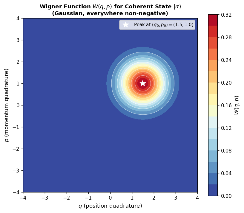 This is such a good approximation that it is often not mentioned in first courses in quantum mechanics that the Schrödinger equation with a classical electromagnetic potential is in fact an approximation — the true description involves two interacting quantum systems that happen not to entangle.
This approximation breaks down for non-classical light — electromagnetic fields not in coherent states. When non-classical light interacts with matter, genuine entanglement is generated and the electron’s state becomes mixed. This is the domain of quantum optics, where phenomena like quantum cryptography, quantum key distribution, and quantum computing with photons live.
10.5.4 The Deep Lesson
The problem is: the same reactivity that makes two qubits interact usefully for computation also makes them reactive with stray electrons, stray photons, and vibrations from the environment. As Kempf puts it, every time a stray electron comes in from the side and scatters off our quantum processor, a measurement is performed — the processor’s pure state becomes mixed, its quantum information is degraded. This is decoherence. It is not a new law; it is just the Schrödinger equation applied to a bigger system than we intended. But its practical consequences are enormous: decoherence is the primary obstacle to building large-scale quantum computers. The solution Kempf suggests is to learn to transform quantum information between physical encodings that are inert to the environment (like photon polarization, which travels far without being disturbed) and encodings that are reactive and can perform gate operations (like ions, which interact strongly with each other but also with the environment). The fundamental physics is the same decoherence mechanism throughout.
Chapter 11. The EPR Paradox and Bell’s Theorem
11.1 Bell States
Before entering the conceptual labyrinth of EPR, we introduce the states at its heart. The four Bell states are the maximally entangled orthonormal basis of the two-qubit Hilbert space:
\[ |\Phi^\pm\rangle = \frac{1}{\sqrt{2}}\bigl(|00\rangle \pm |11\rangle\bigr), \qquad |\Psi^\pm\rangle = \frac{1}{\sqrt{2}}\bigl(|01\rangle \pm |10\rangle\bigr). \]These four states are orthonormal and span all of \(\mathcal{H}_A \otimes \mathcal{H}_B\), forming a complete basis called the Bell basis. They will reappear as the central actors in both Bell’s theorem and quantum teleportation.
11.2 The Einstein-Podolsky-Rosen Argument
In 1935, Einstein, Podolsky, and Rosen published a paper entitled “Can Quantum-Mechanical Description of Physical Reality Be Considered Complete?” that exposed a profound tension between quantum mechanics and what they regarded as physical common sense.
Consider the Bell state \(|\Phi^+\rangle = \frac{1}{\sqrt{2}}(|00\rangle + |11\rangle)\). Neither qubit has a definite value of \(\hat{\sigma}_z\) — they are genuinely in superposition. Yet if Alice measures her qubit and obtains \(|0\rangle\), the state of the joint system collapses:
\[ \frac{\hat{P}_{|0_A\rangle}|\Phi^+\rangle}{\|\hat{P}_{|0_A\rangle}|\Phi^+\rangle\|} = |0_A 0_B\rangle. \]Bob’s qubit is instantaneously projected to \(|0_B\rangle\), regardless of how far away Bob is. From a strict Copenhagen perspective, something seems to have propagated instantaneously across arbitrarily large distances — in apparent contradiction with relativity.
EPR offered two possible explanations: either there is an instantaneous non-local interaction between the particles (which they considered unacceptable), or the outcome of any measurement on Bob’s qubit was predetermined by some pre-existing information carried by the particles — so-called hidden variables. EPR preferred the hidden-variable interpretation, concluding that quantum mechanics was an incomplete description of reality because its formalism had no room for such pre-existing values.
The discussion remained philosophical for nearly three decades, until John Bell showed in 1964 that the hidden-variable hypothesis was not merely a philosophical preference but a testable physical claim — one that makes quantitative predictions that quantum mechanics violates.
11.3 Bell’s Theorem and the CHSH Inequality
Bell’s insight was to derive a mathematical inequality that any local hidden-variable theory must satisfy. We follow the Clauser-Horne-Shimony-Holt (CHSH) form.
Setting up local realism. Consider two qubits in spacelike-separated regions. Alice can choose between measurement settings \(a\) or \(a'\), Bob between \(b\) or \(b'\), with outcomes \(\pm 1\). Local realism asserts that there exist functions \(A(a, \lambda) = \pm 1\) and \(B(b, \lambda) = \pm 1\), where \(\lambda\) denotes hidden variables distributed according to some probability density \(\Lambda(\lambda)\) with \(\int\Lambda(\lambda)\,d\lambda = 1\), and crucially \(A\) does not depend on \(b\) and \(B\) does not depend on \(a\) (locality). The correlation function is
\[ C(a, b) = \int A(a,\lambda)\,B(b,\lambda)\,\Lambda(\lambda)\,d\lambda. \]The proof is a short algebraic exercise. From the identity
\[ C(a,b) - C(a,b') = \int A(a,\lambda)\,B(b,\lambda)\bigl[1 \pm A(a',\lambda)B(b',\lambda)\bigr]\,\Lambda(\lambda)\,d\lambda - \int A(a,\lambda)\,B(b',\lambda)\bigl[1 \pm A(a',\lambda)B(b,\lambda)\bigr]\,\Lambda(\lambda)\,d\lambda, \]and using \(|A|, |B| \leq 1\) together with \(\int\Lambda\,d\lambda = 1\), one arrives at
\[ \bigl|C(a,b) - C(a,b')\bigr| \leq 2 \pm \bigl[C(a',b') + C(a',b)\bigr]. \]Taking the appropriate sign gives the CHSH inequality. This is a necessary condition for local realism, satisfied by any theory with pre-defined outcomes and no faster-than-light influences.
11.4 Quantum Violation: \(2\sqrt{2} > 2\)
Quantum mechanics can violate the CHSH inequality. Consider the Bell state \(|\Psi^-\rangle = \frac{1}{\sqrt{2}}(|01\rangle - |10\rangle)\). Alice measures along \(\hat{\sigma}_z\) (setting \(a\)) or \(\hat{\sigma}_x\) (setting \(a'\)). Bob measures along settings \(b = -\frac{1}{\sqrt{2}}(\hat{\sigma}_z + \hat{\sigma}_x)\) and \(b' = \frac{1}{\sqrt{2}}(\hat{\sigma}_z - \hat{\sigma}_x)\).
Computing all four correlators on \(|\Psi^-\rangle\),
\[ \langle A(a)B(b)\rangle = \langle A(a')B(b')\rangle = \langle A(a')B(b)\rangle = -\langle A(a)B(b')\rangle = \frac{1}{\sqrt{2}}. \]Substituting into the left-hand side of the CHSH inequality:
\[ \left|\frac{1}{\sqrt{2}} - \frac{1}{\sqrt{2}}\right| + \left|\frac{1}{\sqrt{2}} + \frac{1}{\sqrt{2}}\right| = 0 + \frac{2}{\sqrt{2}} + \frac{2}{\sqrt{2}} = 2\sqrt{2} \approx 2.83 > 2. \]This is one of the most important results in physics. It means that no theory of pre-existing hidden variables, subject to Einstein’s locality, can reproduce all the predictions of quantum mechanics. The EPR proposal was not just incomplete — it was demonstrably wrong. Alain Aspect and collaborators experimentally confirmed the violation of Bell inequalities in 1982, closing the most significant experimental loopholes.
11.5 No-Signalling: Entanglement Cannot Transmit Information
The Bell violation might seem alarming from the perspective of relativity: something non-local is going on. But the crucial observation is that entanglement cannot be used to signal faster than light.
When Alice measures her qubit, she gets a random outcome \(\pm 1\) with equal probability, regardless of her choice of setting and regardless of what Bob does. Bob’s reduced state \(\hat{\rho}_B = \operatorname{Tr}_A(|\Psi^-\rangle\langle\Psi^-|) = \frac{1}{2}\mathbb{1}\) is maximally mixed no matter what Alice does. Bob cannot detect any change in his local statistics caused by Alice’s choice of measurement — the correlations between their outcomes only become apparent when they compare results through a classical channel, which is limited by the speed of light.
Chapter 12. Measures of Entanglement
12.1 Separable and Entangled States
We now formalize the notion of entanglement for general (possibly mixed) bipartite states.
The intuition is clear: a separable state has correlations that could in principle be explained by a shared classical strategy (the mixture over \(i\)), while an entangled state has correlations that exceed what any such classical strategy can achieve.
For pure states, separability takes the simpler form \(|\psi_{AB}\rangle = |\psi_A\rangle \otimes |\psi_B\rangle\). The Bell state \(|\Phi^+\rangle = \frac{1}{\sqrt{2}}(|00\rangle + |11\rangle)\) is entangled: there are no single-qubit states whose tensor product gives it. Conversely, the state \(\frac{1}{2}(|0\rangle + |1\rangle)_A \otimes (|0\rangle + |1\rangle)_B\) is separable. The partial trace test distinguishes them: the reduced state \(\hat{\rho}_A\) for the entangled Bell state is the maximally mixed state \(\frac{1}{2}\mathbb{1}\), while for the separable state it is a pure state.
If \(|\Omega\rangle_{AB}\) is unentangled (i.e., it is a product state \(|\psi\rangle_A \otimes |\phi\rangle_B\)), then both subsystem states are pure: \(\hat{\rho}_A = |\psi\rangle\langle\psi|\) and \(\hat{\rho}_B = |\phi\rangle\langle\phi|\). And conversely.
If \(|\Omega\rangle_{AB}\) is entangled, then both subsystem states are mixed. The more entangled the state, the more mixed the subsystems. And conversely.
Kempf’s way of saying it: “Purity of the subsystems goes hand in hand with un-entanglement of the super-system. Mixedness of the subsystems is an expression of there being entanglement in the super-system. Keep that in mind — entanglement in the big system means mixedness of the small systems.”
This duality is the foundation of the entanglement entropy: to measure how entangled \(A\) and \(B\) are in the full system, simply measure how mixed subsystem \(A\) is. If it is pure, they are not entangled. The more mixed it is, the more they are entangled.
12.2 Axioms for Entanglement Measures
Since there is no unique measure of entanglement, a measure of entanglement is any function \(E(\hat{\rho})\) satisfying:
- \(E(\hat{\rho}) = 0\) for all separable states.
- \(E(\hat{\rho}) > 0\) for all non-separable states.
- \(E(\hat{\rho})\) is maximal for maximally entangled states (Bell states for two qubits).
- \(E(\hat{\rho})\) cannot increase under local operations and classical communication (LOCC) — entanglement cannot be created by operations that involve only local manipulations of each subsystem and the exchange of classical information between parties.
The LOCC monotonicity condition is the physically essential one: if entanglement could increase under LOCC, it would be a free resource, which contradicts its role as a non-classical correlation. In practice, the hardness of computing entanglement measures for general mixed states of arbitrary dimension is a major open problem.
12.3 Entanglement Entropy
For pure bipartite states, the Von Neumann entropy of either reduced state provides a natural and elegant entanglement measure.
The entanglement entropy is zero if and only if the state is a product state (then \(\hat{\rho}_A\) is pure), and it reaches its maximum value \(\log d\) for maximally entangled states (then \(\hat{\rho}_A = \frac{1}{d}\mathbb{1}\)). For the Bell state \(|\Phi^+\rangle\), the partial state is \(\hat{\rho}_A = \frac{1}{2}\mathbb{1}\) and \(S_\text{ent} = \log 2 = 1\) bit.
An important caveat: the entanglement entropy is a valid measure only for pure joint states. For mixed states it fails to satisfy the LOCC axiom: a mixed state may have a large \(S(\hat{\rho}_A)\) for reasons unrelated to entanglement (classical correlations, noise, etc.). For mixed states, one must use other measures such as the negativity or the entanglement of formation.
This holds regardless of how different \(\mathcal{H}_A\) and \(\mathcal{H}_B\) are (they can have different dimensions). The Schmidt number — the number of non-zero \(\lambda_i\) — measures the “amount” of entanglement: the state is a product state if and only if exactly one Schmidt coefficient is non-zero (Schmidt rank 1), in which case both entropies vanish.
12.4 The Peres Criterion and Negativity
The most practically useful criterion for detecting entanglement in finite-dimensional systems is the partial transpose criterion, introduced by Peres in 1996.
For a bipartite density matrix written in the product basis as \(\hat{\rho}_{AB} = \sum_{ijkl}\rho_{ijkl}|i\rangle_A|j\rangle_B\langle k|_A\langle l|_B\), the partial transpose with respect to \(B\) is
\[ (\hat{\rho}_{AB}^{T_B})_{ij,kl} = \rho_{il,kj}, \]corresponding to transposing only the \(B\) indices while leaving the \(A\) indices unchanged.
For higher-dimensional systems, a negative eigenvalue of the partial transpose is still sufficient for entanglement, but not necessary: bound entangled states exist in higher dimensions — states that are entangled, yet whose partial transpose is positive semidefinite, and whose entanglement cannot be distilled into pure Bell pairs by any LOCC protocol. For the physically most relevant cases (two qubits and qubit-qutrit systems), however, the Peres criterion is both necessary and sufficient.
Based on the Peres criterion, the negativity provides a computable entanglement monotone:
The negativity is zero for separable states and reaches a maximum of \(\mathcal{N}_{\max} = 1/2\) for maximally entangled two-qubit states. It is an LOCC monotone and is sensitive to distillable entanglement.
12.5 Concurrence and Entanglement of Formation
For two-qubit systems, another widely used measure is the concurrence, which has the advantage of a closed-form expression for arbitrary two-qubit states.
The concurrence is 0 for separable states and 1 for maximally entangled Bell states. In the two-qubit case, concurrence and negativity are related by the inequality
\[ \mathcal{C} > 2\mathcal{N} > \sqrt{(1-\mathcal{C})^2 + \mathcal{C}^2} - (1-\mathcal{C}). \]The entanglement of formation \(E_F\) gives the concurrence an operational meaning: it quantifies the minimum average number of maximally entangled qubit pairs (ebits) needed to prepare \(\hat{\rho}\) by LOCC:
\[ E_F(\hat{\rho}_{AB}) = h\!\left(\frac{1 + \sqrt{1 - \mathcal{C}(\hat{\rho})^2}}{2}\right), \]where \(h(x) = -x\log_2 x - (1-x)\log_2(1-x)\) is the binary entropy function. This gives entanglement in units of ebits (maximally entangled pairs), making it directly interpretable as a resource quantity.
12.6 Mutual Information and Total Correlations
Entanglement measures only capture purely quantum correlations. A complementary quantity that captures all correlations — both classical and quantum — is the quantum mutual information.
The mutual information generalizes the classical mutual information \(I(X;Y) = H(X) + H(Y) - H(X,Y)\) to the quantum domain. It is zero if and only if the state is a product state \(\hat{\rho}_{AB} = \hat{\rho}_A \otimes \hat{\rho}_B\) (no correlations whatsoever), and is positive for any correlated state, including classically correlated but separable states. This makes it useful as a diagnostic tool: one can compare \(I_{AB}\) with an entanglement measure to assess what fraction of the total correlations are quantum in nature. In a purely classically correlated state, the entanglement is zero but \(I_{AB}\) may still be positive; in a maximally entangled state, \(I_{AB}\) reaches its maximum of \(2\log d\).
Chapter 13. Quantum Teleportation
13.1 Overview and Historical Context
Quantum teleportation is perhaps the most dramatic demonstration that entanglement is a genuine physical resource. It is a protocol by which the complete quantum state of a particle can be transmitted from one location to another using only a shared entangled pair and a two-bit classical message — without the quantum information itself ever travelling through the classical channel.
The protocol was proposed in 1993 by Bennett, Brassard, Crépeau, Jozsa, Peres, and Wootters, and first experimentally demonstrated in 1997 by Bouwmeester and collaborators. It is foundational in quantum communication, quantum networks, and quantum computing.
The name “teleportation” is vivid but must be understood carefully: no matter is transported, and no information travels faster than light. The classical channel is indispensable — without it, the protocol fails, and causality is preserved absolutely.
13.2 The Protocol
We present the teleportation protocol step by step for a single qubit.
Step 0 — Entanglement distribution. Alice and Bob share the Bell pair
\[ |\Phi^+\rangle_{A_2 B_3} = \frac{1}{\sqrt{2}}\bigl(|00\rangle_{A_2 B_3} + |11\rangle_{A_2 B_3}\bigr). \]Bob departs to a distant location, taking qubit \(B_3\) with him. Alice is then given a qubit \(|\varphi\rangle_{A_1} = \alpha_0|0\rangle + \alpha_1|1\rangle\) whose state she does not know and wants to transmit to Bob.
Step 1 — Writing the full state. The initial state of all three qubits is
\[ |\psi\rangle_{A_1 A_2 B_3} = |\varphi\rangle_{A_1} \otimes |\Phi^+\rangle_{A_2 B_3} = \frac{1}{\sqrt{2}}\bigl(\alpha_0|000\rangle + \alpha_0|011\rangle + \alpha_1|100\rangle + \alpha_1|111\rangle\bigr)_{A_1 A_2 B_3}. \]Step 2 — Rewriting in the Bell basis. Alice will measure her two qubits \(A_1 A_2\) in the Bell basis. To see the outcome, we rewrite \(|00\rangle, |01\rangle, |10\rangle, |11\rangle\) in the Bell basis:
\[ |00\rangle = \frac{1}{\sqrt{2}}\bigl(|\Phi^+\rangle + |\Phi^-\rangle\bigr), \quad |11\rangle = \frac{1}{\sqrt{2}}\bigl(|\Phi^+\rangle - |\Phi^-\rangle\bigr), \]\[ |01\rangle = \frac{1}{\sqrt{2}}\bigl(|\Psi^+\rangle + |\Psi^-\rangle\bigr), \quad |10\rangle = \frac{1}{\sqrt{2}}\bigl(|\Psi^+\rangle - |\Psi^-\rangle\bigr). \]Substituting these into the tripartite state and collecting terms:
\[ |\psi\rangle_{A_1 A_2 B_3} = \frac{1}{2}\Bigl[ |\Phi^+\rangle_{A_1 A_2}\otimes(\alpha_0|0\rangle + \alpha_1|1\rangle)_{B_3} + |\Phi^-\rangle_{A_1 A_2}\otimes(\alpha_0|0\rangle - \alpha_1|1\rangle)_{B_3} \]\[ + |\Psi^+\rangle_{A_1 A_2}\otimes(\alpha_0|1\rangle + \alpha_1|0\rangle)_{B_3} + |\Psi^-\rangle_{A_1 A_2}\otimes(\alpha_0|1\rangle - \alpha_1|0\rangle)_{B_3} \Bigr]. \]Each Bell state of Alice’s two qubits occurs with equal probability \(1/4\), and conditioned on Alice’s measurement outcome, Bob’s qubit is projected into one of four states.
Step 3 — Alice’s Bell measurement and classical communication. Alice measures her two qubits jointly in the Bell basis, obtaining one of the four Bell states with equal probability \(1/4\). She sends her two-bit outcome to Bob through a classical channel. Bob receives the 2 classical bits and applies the appropriate local unitary:
| Alice measures | Bob’s state | Bob applies | Result |
|---|---|---|---|
| \(\|\Phi^+\rangle\) | \(\alpha_0\|0\rangle + \alpha_1\|1\rangle\) | \(\mathbb{1}\) (nothing) | \(\|\varphi\rangle\) |
| \(\|\Phi^-\rangle\) | \(\alpha_0\|0\rangle - \alpha_1\|1\rangle\) | \(\hat{\sigma}_z\) | \(\|\varphi\rangle\) |
| \(\|\Psi^+\rangle\) | \(\alpha_0\|1\rangle + \alpha_1\|0\rangle\) | \(\hat{\sigma}_x\) | \(\|\varphi\rangle\) |
| \(\|\Psi^-\rangle\) | \(\alpha_0\|1\rangle - \alpha_1\|0\rangle\) | \(i\hat{\sigma}_y\) | \(\|\varphi\rangle\) |
In every case, Bob recovers \(|\varphi\rangle_{B_3} = \alpha_0|0\rangle + \alpha_1|1\rangle\), the original unknown state. Teleportation is complete.
13.3 Key Features and Causality
Several features of the teleportation protocol deserve emphasis:
No cloning. At the end of the protocol, the original qubit \(A_1\) no longer carries the state \(|\varphi\rangle\) — the Bell measurement on \(A_1 A_2\) destroys the original state. This is consistent with the no-cloning theorem, which states that no physical operation can produce a perfect copy of an unknown quantum state. Teleportation is the transfer, not the copy, of a quantum state.
Classical channel is essential. Before Bob receives Alice’s 2-bit message, his qubit \(B_3\) is in one of the four states in the table above, each equally likely. His reduced density matrix is \(\hat{\rho}_{B_3} = \frac{1}{2}\mathbb{1}\) — the maximally mixed state — regardless of the unknown \(|\varphi\rangle\). He cannot extract any information about \(|\varphi\rangle\) without Alice’s classical message. The classical channel is not a technicality; it is physically essential, and it is limited by the speed of light.
Causality is preserved. No information about \(|\varphi\rangle\) reaches Bob before the classical message arrives. The entanglement provides a non-local quantum correlation, but that correlation is invisible to Bob alone. Only after combining his quantum state with Alice’s classical information can he reconstruct \(|\varphi\rangle\). There is no faster-than-light communication.
Block 3 summary: The density operator \(\hat{\rho} = \sum_i p_i|\varphi_i\rangle\langle\varphi_i|\) is the fundamental object describing states with classical uncertainty; pure states satisfy \(\operatorname{Tr}\hat{\rho}^2 = 1\) while mixed states have \(\operatorname{Tr}\hat{\rho}^2 < 1\). Thermal equilibrium at inverse temperature \(\beta\) is described by the Gibbs state \(\hat{\rho}_\beta = e^{-\beta\hat{H}}/Z\), which coincides with KMS states whenever both are defined; the KMS condition extends the notion of thermality to infinite systems where the partition function diverges. Bipartite systems are described in \(\mathcal{H}_A\otimes\mathcal{H}_B\), with reduced states obtained by partial trace. Bell’s theorem shows that no local hidden-variable theory can reproduce quantum correlations: the CHSH inequality \(|C(a,b)-C(a,b')| + |C(a',b')+C(a',b)| \leq 2\) is violated by quantum mechanics, which achieves \(2\sqrt{2}\). Entanglement is quantified by the entanglement entropy (for pure states), negativity, concurrence, and entanglement of formation; mutual information captures total correlations. Quantum teleportation demonstrates entanglement as a resource: an unknown qubit state can be transmitted using a shared Bell pair and 2 classical bits, with causality preserved throughout.
Part IV — Quantum Dynamics
Chapter 14. Unitarity and Pictures of Quantum Mechanics
§14.1 — The Time Evolution Operator and Unitarity
Time-dependent quantum mechanics begins with the Schrödinger equation. Rather than assuming from the outset that evolution is unitary, we derive that property from the self-adjointness of the Hamiltonian. Begin with
\[ i \frac{d}{dt} |\psi(t)\rangle = \hat{H}(t) |\psi(t)\rangle \](setting \( \hbar = 1 \) throughout). Given an initial condition \( |\psi(t_0)\rangle \), the solution at any later time must be some linear transformation of the initial state — the linearity of the equation guarantees this. We write
\[ |\psi(t)\rangle = \hat{U}(t, t_0) |\psi(t_0)\rangle \]and discover that the time evolution operator \( \hat{U}(t, t_0) \) satisfies exactly the same equation:
\[ i \frac{d}{dt} \hat{U}(t, t_0) = \hat{H}(t) \hat{U}(t, t_0), \qquad \hat{U}(t_0, t_0) = \mathbf{1}. \]The proof is direct. Differentiate \( \hat{U}\hat{U}^\dagger \) with respect to time and use the equation of motion:
\[ \frac{\partial}{\partial t}\!\left(\hat{U}\hat{U}^\dagger\right) = \frac{\partial \hat{U}}{\partial t}\hat{U}^\dagger + \hat{U}\frac{\partial \hat{U}^\dagger}{\partial t} = \frac{-i}{\hbar}\hat{H}\hat{U}\hat{U}^\dagger + \hat{U}\hat{U}^\dagger \frac{i}{\hbar}\hat{H}^\dagger. \]Since \( \hat{H} = \hat{H}^\dagger \), the two terms cancel and \( \partial_t(\hat{U}\hat{U}^\dagger) = 0 \). Combined with the initial condition \( \hat{U}(t_0, t_0) = \mathbf{1} \), this gives \( \hat{U}\hat{U}^\dagger = \mathbf{1} \) for all time, so \( \hat{U}^\dagger = \hat{U}^{-1} \).
When \( \hat{H} \) is time-independent the equation for \( \hat{U} \) has the closed-form solution
\[ \hat{U}(t, t_0) = e^{-i(t - t_0)\hat{H}}. \]This is manifestly unitary. When \( \hat{H} \) depends on time there is no such simple closed form — the operators at different times generally do not commute — and we must work harder, as the Dyson series of Chapter 14 shows.
§14.2 — Two Pictures: Schrödinger and Heisenberg
The physically meaningful quantities in quantum mechanics are probability distributions of observables, not the abstract state vectors or operators themselves. The expectation value of an observable \( \hat{O} \) at time \( t \) is
\[ \langle \hat{O} \rangle_t = \langle \psi(t) | \hat{O} | \psi(t) \rangle = \langle \psi(t_0) | \hat{U}^\dagger(t, t_0)\, \hat{O}\, \hat{U}(t, t_0) | \psi(t_0) \rangle. \]This single expression admits two completely equivalent interpretations, leading to the two fundamental pictures of quantum mechanics. The key insight is that physical content lives in the combination \( \hat{U}^\dagger \hat{O} \hat{U} \) — we may assign the time dependence to either factor.
The expectation value reads \( \langle \hat{O} \rangle_t = \langle \psi(t_0)|\hat{O}_H(t)|\psi(t_0)\rangle \) in the Heisenberg picture — identical to the Schrödinger picture result, as it must be.
Differentiating the definition of \( \hat{O}_H \) and using the equation of motion for \( \hat{U} \) gives the Heisenberg equation of motion:
\[ \frac{d\hat{O}_H}{dt} = i\bigl[\hat{H}_H, \hat{O}_H\bigr] + \left(\frac{\partial \hat{O}}{\partial t}\right)_H, \]where \( \hat{H}_H = \hat{U}^\dagger \hat{H} \hat{U} \) and the last term is nonzero only if \( \hat{O} \) carries an explicit time dependence beyond that generated by dynamics. Both pictures yield the same equation for \( \frac{d}{dt}\langle O \rangle_t \):
\[ \frac{d}{dt}\langle O \rangle_t = \frac{i}{\hbar}\left\langle \bigl[\hat{H}, \hat{O}\bigr] \right\rangle_t + \left\langle \frac{\partial \hat{O}}{\partial t} \right\rangle_t. \]§14.3 — The Interaction (Dirac) Picture
The Schrödinger and Heisenberg pictures are the two extremes: all time dependence in the states, or all in the operators. A third possibility, particularly tailored for perturbation theory, is the interaction picture (also called the Dirac picture), in which both states and operators evolve, but in a controlled way.
The setting is a Hamiltonian split into a time-independent free part and a (possibly time-dependent) interaction:
\[ \hat{H} = \hat{H}_0 + \lambda \hat{V}(t). \]Define the unitary operator \( \hat{U}_0 \equiv e^{i\hat{H}_0 t} \) and the interaction-picture state and operators by
\[ |\psi(t)\rangle_D = \hat{U}_0 |\psi(t)\rangle_S, \qquad \hat{O}_D(t) = \hat{U}_0 \hat{O}_S \hat{U}_0^\dagger. \]The subscript \( D \) stands for Dirac and \( S \) for Schrödinger. A short calculation — substituting into the Schrödinger equation, using \( \partial_t \hat{U}_0^\dagger = -i\hat{H}_0 \hat{U}_0^\dagger \), and noting that \( \hat{H}_{0D} = \hat{H}_0 \) because \( \hat{H}_0 \) commutes with every function of itself — yields cancellation of the free-evolution terms on both sides, leaving
\[ i \frac{d}{dt}|\psi(t)\rangle_D = \lambda \hat{V}_D(t) |\psi(t)\rangle_D. \]The operators therefore oscillate at the free-theory frequencies, while the states carry the perturbative corrections. This clean separation is exactly what makes the interaction picture the natural arena for perturbation theory.
A critical caveat: the separation between free and interacting evolution cannot be made multiplicative in general. Even for a time-independent Hamiltonian,
\[ e^{-i(\hat{H}_0 + \lambda\hat{V})t} \;\neq\; e^{-i\hat{H}_0 t} e^{-i\lambda\hat{V} t} \]unless \( [\hat{H}_0, \hat{V}] = 0 \). Handwaving descriptions of the interaction picture as “removing free evolution and watching only the interaction” must be taken with care.
§14.4 — A Fourth Perspective: The Green’s Function and the Propagator
Crucially, this is a solution for all initial conditions simultaneously — a single computation of \( G \) unlocks the full dynamics of the system.
\[ i\hbar\,\frac{\partial}{\partial t}G(x, x', t) = \hat{H}\!\left(x,\, -i\hbar\frac{\partial}{\partial x}\right) G(x, x', t), \qquad G(x, x', t_0) = \delta(x - x'). \]The Schrödinger equation is therefore nothing more than the differential equation that the propagator satisfies. The delta-function initial condition encodes the statement that a particle sharply localized at \( x' \) at time \( t_0 \) is a point source propagating forward.
\[ G(x, x', t) = \sqrt{\frac{m\omega}{2\pi i\hbar\sin(\omega t)}}\exp\!\left(\frac{im\omega}{2\hbar\sin(\omega t)}\bigl[(x^2 + x'^2)\cos(\omega t) - 2xx'\bigr]\right). \]At \( t = \pi/(2\omega) \) (one quarter period), \( \cos(\omega t) = 0 \) and the Green’s function reduces to a pure Fourier kernel: the harmonic oscillator Fourier-transforms its own wavefunction in a quarter period. This is exploited in quantum computing (e.g. Shor’s algorithm for integer factoring) as a physically realised fast Fourier transform.
This Green’s function perspective sets up the path integral: instead of solving for \( G \) via the differential equation above, Feynman found an entirely different formula — a sum over all paths — which is developed in Chapter 18.
Chapter 15. Time-Dependent Perturbation Theory and the Dyson Series
§15.1 — The Dyson Series
In the interaction picture, the time evolution operator \( \hat{U}_D(t, t_0) \) defined by \( |\psi(t)\rangle_D = \hat{U}_D(t, t_0)|\psi(t_0)\rangle_D \) satisfies
\[ \frac{d}{dt}\hat{U}_D(t, t_0) = -i\lambda \hat{V}_D(t) \hat{U}_D(t, t_0), \qquad \hat{U}_D(t_0, t_0) = \mathbf{1}. \]If \( \hat{V}_D(t) \) commuted with itself at all times, the solution would be the simple exponential \( \exp\!\bigl(-i\lambda \int_{t_0}^t \hat{V}_D(t')\,dt'\bigr) \). But operators at different times generically do not commute. We must instead convert the differential equation into an integral equation:
\[ \hat{U}_D(t, t_0) = \mathbf{1} - i\lambda \int_{t_0}^t dt_1\, \hat{V}_D(t_1)\, \hat{U}_D(t_1, t_0). \]Substituting the right-hand side recursively into itself generates the Dyson series:
\[ \hat{U}_D(t, t_0) = \mathbf{1} + \hat{U}_D^{(1)} + \hat{U}_D^{(2)} + \hat{U}_D^{(3)} + \cdots \]where the successive terms are
\[ \hat{U}_D^{(1)}(t,t_0) = -i\lambda \int_{t_0}^t dt_1\, \hat{V}_D(t_1), \]\[ \hat{U}_D^{(2)}(t,t_0) = (-i\lambda)^2 \int_{t_0}^t dt_1 \int_{t_0}^{t_1} dt_2\, \hat{V}_D(t_1)\hat{V}_D(t_2), \]\[ \hat{U}_D^{(3)}(t,t_0) = (-i\lambda)^3 \int_{t_0}^t dt_1 \int_{t_0}^{t_1} dt_2 \int_{t_0}^{t_2} dt_3\, \hat{V}_D(t_1)\hat{V}_D(t_2)\hat{V}_D(t_3). \]The nested integration limits enforce the crucial ordering \( t \geq t_1 \geq t_2 \geq t_3 \geq \cdots \geq t_0 \): at each level, operators at earlier times act before operators at later times, which is the correct causal structure.
This series is compactly written using the time-ordering operator \( \mathcal{T} \):
\[ \hat{U}_D(t, t_0) = \mathcal{T}\exp\!\left(-i\lambda\int_{t_0}^t \hat{V}_D(t')\,dt'\right). \]§15.2 — The Hadamard Lemma
A key technical tool for computing interaction-picture operators is the following identity.
This is proved by differentiating \( f(x) = e^{x\hat{A}}\hat{B}e^{-x\hat{A}} \) repeatedly and recognising that \( f^{(n)}(0) \) is the \(n\)-fold nested commutator of \( \hat{A} \) with \( \hat{B} \).
§15.3 — Extended Example: Detector Coupled to Field Modes
To illustrate the Dyson series concretely, consider \( N+1 \) quantum harmonic oscillators: one detector (labeled 0) linearly coupled to \( N \) field modes. In terms of position and momentum operators with masses \( m_n \) and frequencies \( \omega_n \), and with \( \kappa = \lambda\sqrt{2m_0\omega_0} \), this system is described by
\[ \hat{H} = \omega_0 \hat{a}_0^\dagger \hat{a}_0 + \sum_{n=1}^N \omega_n \hat{a}_n^\dagger \hat{a}_n + \lambda(\hat{a}_0 + \hat{a}_0^\dagger)\sum_{n=1}^N \frac{1}{\sqrt{2\omega_n m_n}}(\hat{a}_n + \hat{a}_n^\dagger) + E_Z\mathbf{1}, \]where \( [\hat{a}_n, \hat{a}_m^\dagger] = \delta_{nm} \) and \( E_Z \) is the (finite, for \( N < \infty \)) zero-point energy, which we absorb into the origin of energies. We split \( \hat{H} = \hat{H}_0 + \lambda\hat{V} \) with
\[ \hat{H}_0 = \omega_0 \hat{a}_0^\dagger \hat{a}_0 + \sum_n \omega_n \hat{a}_n^\dagger \hat{a}_n, \qquad \hat{V} = (\hat{a}_0 + \hat{a}_0^\dagger)\sum_n \frac{\hat{a}_n + \hat{a}_n^\dagger}{\sqrt{2\omega_n m_n}}. \]To find \( \hat{V}_D \) we conjugate by \( \hat{U}_0 = e^{i\hat{H}_0 t} \). Applying the Hadamard lemma to the annihilation operator, using \( [\hat{a}_n^\dagger \hat{a}_n, \hat{a}_n] = -\hat{a}_n \), gives
\[ e^{i\omega_n t \hat{a}_n^\dagger \hat{a}_n}\,\hat{a}_n\,e^{-i\omega_n t \hat{a}_n^\dagger \hat{a}_n} = e^{-i\omega_n t}\hat{a}_n, \]and similarly \( e^{i\omega_n t \hat{a}_n^\dagger \hat{a}_n}\hat{a}_n^\dagger e^{-i\omega_n t \hat{a}_n^\dagger \hat{a}_n} = e^{i\omega_n t}\hat{a}_n^\dagger \). Therefore
\[ \hat{V}_D(t) = \bigl(\hat{a}_0 e^{-i\omega_0 t} + \hat{a}_0^\dagger e^{i\omega_0 t}\bigr)\sum_n \frac{\hat{a}_n e^{-i\omega_n t} + \hat{a}_n^\dagger e^{i\omega_n t}}{\sqrt{2\omega_n m_n}}. \]At first order in \( \lambda \), the evolution operator \( \hat{U}_D^{(1)} \) contains four types of terms after expanding the product:
\[ \hat{U}_D^{(1)}(t,0) = -i\lambda\sum_n \frac{1}{\sqrt{2\omega_n m_n}}\int_0^t dt_1 \Bigl[ \hat{a}_0\hat{a}_n^\dagger e^{-i(\omega_0 - \omega_n)t_1} + \hat{a}_0^\dagger\hat{a}_n e^{i(\omega_0-\omega_n)t_1} + \hat{a}_0\hat{a}_n e^{-i(\omega_0+\omega_n)t_1} + \hat{a}_0^\dagger\hat{a}_n^\dagger e^{i(\omega_0+\omega_n)t_1} \Bigr]. \]The first two terms involve one excitation and one de-excitation; the last two create or destroy two excitations simultaneously.
To understand when each type of term dominates, examine the time integral weighting each. A rotating-wave term carries the factor
\[ \int_0^t dt_1\, e^{i(\omega_0 - \omega_n)t_1}. \]For a non-resonant mode \( \omega_n \neq \omega_0 \), this integral is bounded by \( (\omega_0 - \omega_n)^{-1} \) as \( t \to \infty \), while for the resonant mode \( \omega_n = \omega_0 \) it grows as \( t \). At long times, the resonant contribution dominates all non-resonant ones — the single-mode approximation consists of keeping only the resonant contribution.
A counter-rotating term carries \( \int_0^t dt_1 \, e^{i(\omega_0+\omega_n)t_1} \), which is bounded by \( (\omega_0 + \omega_n)^{-1} \) for all \( \omega_n > 0 \). For times \( \Delta T \gg (\omega_0 + \omega_n)^{-1} \) this is negligible — this is the rotating-wave approximation (RWA).
Chapter 16. Fermi’s Golden Rule
§16.1 — Transition Probabilities
Return to the general setup \( \hat{H} = \hat{H}_0 + \lambda\hat{V}(t) \) with eigenstates \( \hat{H}_0|n\rangle = E_n|n\rangle \). By Born’s rule, the probability of transitioning from initial state \( |\psi(t_0)\rangle \) to final state \( |\phi\rangle \) is
\[ P_{|\psi\rangle \to |\phi\rangle} = \bigl|\langle \phi | \hat{U}(t, t_0) | \psi(t_0)\rangle\bigr|^2. \]When both the initial and final states are eigenstates of \( \hat{H}_0 \) — say \( |\psi(t_0)\rangle = |n\rangle \) and \( |\phi\rangle = |m\rangle \) — the interaction picture simplifies the calculation significantly. One shows that
\[ \langle m | \hat{U}(t,t_0) | n \rangle = e^{-i(E_m t - E_n t_0)} \langle m | \hat{U}_D(t,t_0) | n \rangle, \]so the transition probability is
\[ P_{n \to m} = \bigl|\langle m | \hat{U}_D(t,t_0) | n \rangle\bigr|^2. \]The complex phase cancels in the squared modulus, so we may freely use the interaction-picture evolution operator and the Schrödinger-picture eigenstates.
Example 1 — Constant perturbation. Suppose \( \hat{V}(t) = \hat{V} \) is switched on at \( t_0 = 0 \) and held constant. In the interaction picture, \( \hat{V}_D = e^{i\hat{H}_0 t}\hat{V}e^{-i\hat{H}_0 t} \), and the first-order transition probability from \( |n\rangle \) to \( |m\rangle \neq |n\rangle \) is
\[ P_{n\to m} = \lambda^2 |V_{mn}|^2 \left|\int_0^t dt_1\, e^{i\omega_{mn} t_1}\right|^2 + O(\lambda^3), \]where \( V_{mn} \equiv \langle m|\hat{V}|n\rangle \) and \( \omega_{mn} = E_m - E_n \). The integral evaluates immediately:
\[ P_{n\to m} = 4\lambda^2 |V_{mn}|^2 \frac{\sin^2(\omega_{mn} t/2)}{\omega_{mn}^2} + O(\lambda^3). \]Example 2 — Harmonic perturbation. For \( \hat{V}(t) = \hat{V}e^{i\Omega t} + \hat{V}^\dagger e^{-i\Omega t} \),
\[ \langle m|\hat{V}_D|n\rangle = V_{mn} e^{i(\omega_{mn}+\Omega)t} + (V^\dagger)_{mn} e^{i(\omega_{mn}-\Omega)t}, \]giving a transition probability involving two competing terms:
\[ P_{n\to m} = \lambda^2 \left| V_{mn}\frac{1 - e^{i(\omega_{mn}+\Omega)t}}{\omega_{mn}+\Omega} + (V^\dagger)_{mn}\frac{1 - e^{i(\omega_{mn}-\Omega)t}}{\omega_{mn}-\Omega} \right|^2. \]In the long-time limit, one term or the other dominates depending on whether \( E_m \approx E_n - \Omega \) (emission) or \( E_m \approx E_n + \Omega \) (absorption).
§16.2 — Fermi’s Golden Rule
When the final state belongs to a continuum, or to a dense set of states with a smooth density, the sum over final states becomes an integral. Define the density of final states \( \rho(E) \) as the number of final states per unit energy interval. The total transition probability to the set \( F \) of final states in \( (E_-, E_+) \) is
\[ P_{n \to F} = \int_{E_-}^{E_+} dE_m\, \rho(E_m)\, P_{n\to m}(E_m). \]For a constant perturbation, substituting the result of Example 1 gives
\[ P_{n \to F} = 4\lambda^2 \int_{E_-}^{E_+} dE_m\, \rho(E_m)\, |V_{mn}|^2\, \frac{\sin^2\!\left(\frac{(E_m - E_n)t}{2}\right)}{(E_m - E_n)^2}. \]The key limit is \( t \to \infty \). One uses the distributional identity
\[ \lim_{t\to\infty} \frac{1}{\pi}\frac{\sin^2(at)}{at^2} = \delta(a), \]or equivalently \( \lim_{t\to\infty} \frac{\sin^2(\omega t/2)}{\omega^2} \sim \frac{\pi t}{2}\delta(\omega) \), to convert the \( \mathrm{sinc}^2 \) peak into a delta function. This yields:
For a harmonic perturbation the two terms in Example 2 each contribute a sinc\(^2\) peak, shifted to \( E_m = E_n \mp \Omega \). In the long-time limit, exactly one of these peaks falls within any finite energy window (the conditions \( E_m = E_n - \Omega \) and \( E_m = E_n + \Omega \) are mutually exclusive for \( \Omega > 0 \)):
- Emission (transition to lower energy \( E_n - \Omega \)): \( P_{n\to F} \approx 2\pi\lambda^2 t\,|V_{mn}|^2\,\rho(E_n - \Omega) \).
- Absorption (transition to higher energy \( E_n + \Omega \)): \( P_{n\to F} \approx 2\pi\lambda^2 t\,|(V^\dagger)_{mn}|^2\,\rho(E_n + \Omega) \).
It is convenient to package these results as the differential transition rate \( w_{n\to m} \) — the transition rate per unit time for a specific final state \( |m\rangle \). Integrating \( w_{n\to m} \) over the density of states recovers the total rate. For a constant perturbation:
\[ w_{n\to m} = 2\pi\lambda^2 |V_{mn}|^2 \delta(E_m - E_n). \]For a harmonic perturbation, emission and absorption rates are respectively
\[ w_{E_n \to E_n - \Omega} = 2\pi\lambda^2 |V_{mn}|^2 \delta(E_m - E_n + \Omega), \]\[ w_{E_n \to E_n + \Omega} = 2\pi\lambda^2 |(V^\dagger)_{mn}|^2 \delta(E_m - E_n - \Omega). \]Chapter 17. Light-Matter Interaction and Selection Rules
§17.1 — The Minimal Coupling Hamiltonian
To describe the interaction of a charged particle with an electromagnetic field we start from the minimal coupling Hamiltonian. An electron of charge \( e \) and mass \( m \) in an electromagnetic field described by vector potential \( A(x) \) and scalar potential \( \phi(x) \) has Hamiltonian (in natural units \( \hbar = c = 1 \))
\[ \hat{H} = \frac{[\hat{p} - eA(\hat{x})]^2}{2m} + e\phi(\hat{x}) = \frac{\hat{p}^2}{2m} - \frac{e}{m}\hat{p}\cdot A(\hat{x}) + \frac{e^2}{2m}[A(\hat{x})]^2 + e\phi(\hat{x}). \]The scalar potential \( \phi \) provides the static Coulomb attraction of the nucleus. The term proportional to \( A^2 \) enters at third order in the coupling \( e/m \) and is dropped for a first-order perturbative analysis. The crucial observation is that \( A(x) \) is a classical field (not a Hermitian operator) satisfying \( \nabla \cdot A = 0 \) (Coulomb gauge), while \( \hat{x} \) is the quantum position operator of the electron.
We take a monochromatic plane wave,
\[ A(x) = 2A_0 \boldsymbol{\epsilon}\cos(\mathbf{k}\cdot\mathbf{x} - \omega t) = A_0\boldsymbol{\epsilon}\Bigl(e^{i(\mathbf{k}\cdot\mathbf{x}-\omega t)} + e^{-i(\mathbf{k}\cdot\mathbf{x}-\omega t)}\Bigr), \]with polarization vector \( \boldsymbol{\epsilon} \), wave vector \( |\mathbf{k}| = \omega \), and \( \mathbf{k}\cdot\boldsymbol{\epsilon} = 0 \). The interaction term then takes the form of a harmonic perturbation
\[ \hat{V}(t) = \hat{V}e^{i\omega t} + \hat{V}^\dagger e^{-i\omega t}, \qquad \hat{V} = -\hat{p}\cdot\boldsymbol{\epsilon}\,e^{-i\mathbf{k}\cdot\hat{x}}, \]with coupling \( \lambda = eA_0/m \). This is precisely the setting of Example 2 above, and Fermi’s Golden Rule applies directly.
Focussing on the absorption process (electron gains energy \( \omega \) from the field), the differential transition rate from atomic state \( |n\rangle \) to state \( |m\rangle \) is
\[ w_{n\to m} = 2\pi \frac{e^2 |A_0|^2}{m^2} \bigl|\langle m | e^{i\mathbf{k}\cdot\hat{x}}\hat{p}\cdot\boldsymbol{\epsilon} | n\rangle\bigr|^2 \delta(E_m - E_n - \omega). \]The absorption cross section — defined as the energy absorbed per unit time divided by the incident energy flux \( \Phi_{\mathrm{EM}} = \omega^2|A_0|^2 / (2\pi) \) — is
\[ \sigma_{\mathrm{abs}} = \frac{4\pi^2 e^2}{m^2 \omega} \bigl|\langle m|e^{i\mathbf{k}\cdot\hat{x}}\hat{p}\cdot\boldsymbol{\epsilon}|n\rangle\bigr|^2 \delta(E_m - E_n - \omega). \]Restoring \( \hbar \) and \( c \) by dimensional analysis (the cross section has dimensions of area), one introduces the fine structure constant \( \alpha = e^2/(4\pi\varepsilon_0 \hbar c) \approx 1/137 \):
\[ \sigma_{\mathrm{abs}} = \frac{4\pi^2\hbar\alpha}{m^2\omega}\bigl|\langle m|e^{i\mathbf{k}\cdot\hat{x}}\hat{p}\cdot\boldsymbol{\epsilon}|n\rangle\bigr|^2 \delta(E_m - E_n - \hbar\omega). \]§17.2 — The Multipole Expansion and Selection Rules
The matrix element \( \langle m | e^{i\mathbf{k}\cdot\hat{x}}\hat{p}\cdot\boldsymbol{\epsilon} | n \rangle \) depends on how the phase \( e^{i\mathbf{k}\cdot x} \) varies across the atom. In typical optical transitions the photon wavelength satisfies \( \lambda_\omega \sim \omega^{-1} \gg a_0 \) (the Bohr radius), so \( |\mathbf{k}\cdot x| \ll 1 \) across the electron wavefunction. We may therefore expand the exponential:
\[ e^{i\mathbf{k}\cdot\hat{x}} = \mathbf{1} + i k_\alpha \hat{x}^\alpha - \frac{1}{2}k_\alpha k_\beta \hat{x}^\alpha \hat{x}^\beta + \cdots \]Substituting term by term into the matrix element \( M = \epsilon^\gamma\langle m|(e^{i\mathbf{k}\cdot\hat{x}})p_\gamma|n\rangle \) gives a hierarchy of multipole contributions.
Electric dipole (E1) — zeroth order. Retaining only \( \mathbf{1} \) in the expansion:
\[ M^{(0)} = \boldsymbol{\epsilon}\cdot\langle m|\hat{p}|n\rangle. \]Using \( [\hat{x}^\gamma, \hat{H}_0] = i\hat{p}^\gamma/m \) (from the canonical commutation relations and \( \hat{H}_0 = \hat{p}^2/2m + e\phi \)), we obtain
\[ \hat{p}^\gamma = -im[\hat{x}^\gamma, \hat{H}_0] \implies M^{(0)} = im(E_m - E_n)\,\boldsymbol{\epsilon}\cdot\langle m|\hat{x}|n\rangle. \]Electric quadrupole (E2) and magnetic dipole (M1) — first order. Retaining the linear term \( ik_\alpha \hat{x}^\alpha \) gives \( M^{(1)} = \epsilon^\gamma k^\alpha \langle m|\hat{x}^\alpha \hat{p}^\gamma|n\rangle \). Symmetrising and antisymmetrising in \( \alpha, \gamma \):
\[ M^{(1)} = \underbrace{\frac{i m(E_m - E_n)}{2}\epsilon^\gamma k^\alpha \langle m|\hat{x}^\alpha\hat{x}^\gamma|n\rangle}_{\mathrm{E2}} + \underbrace{\frac{1}{2}(\mathbf{k}\times\boldsymbol{\epsilon})\cdot\langle m|\hat{x}\times\hat{p}|n\rangle}_{\mathrm{M1}}. \]The E2 term is a matrix element of a rank-2 tensor operator, selecting \( \Delta\ell = 0, \pm 2 \). The M1 term involves the orbital angular momentum \( \hat{L} = \hat{x}\times\hat{p} \), a vector operator selecting \( \Delta\ell = 0, \pm 1 \) (with no parity change, since \( \hat{L} \) is a pseudovector). These transitions are suppressed relative to E1 by a factor of order \( (k\cdot x) \sim a_0/\lambda_\omega \ll 1 \).
so the field does not become entangled with the electron at all — the coupling reduces to a \( c \)-number \( \alpha \) multiplying an operator on the electron alone. Equivalently: when you interact with an eigenstate of your coupling operator, no entanglement is generated, and both subsystems continue to evolve unitarily. The classical field amplitude \( A_0 \) in our formulae is simply \( \alpha \), the eigenvalue.
In practice, laser light and coherent radio-frequency fields are well described by coherent states, for which the field uncertainty \( \Delta(\hat{a}) \) is small relative to the expectation value \( |\alpha| \gg 1 \) (many photons per mode). The field is therefore approximately an eigenstate of \( \hat{a} \), and the semiclassical approximation is excellent. The corrections — arising from photon-number fluctuations and vacuum modes — contribute at the level of \( 1/|\alpha|^2 \) per photon mode and are responsible for the quantum electrodynamical corrections (Lamb shift, spontaneous emission, Casimir effect) suppressed by additional factors of the fine structure constant \( \alpha \approx 1/137 \).
It is precisely when non-classical light is used — squeezed states, Fock states, entangled photon pairs — that this approximation breaks down and the full quantum treatment of the field becomes essential. Such states are at the heart of modern quantum optics, quantum communication, and quantum metrology.
Chapter 18. The Photoelectric Effect
§18.1 — Setup: Bound-to-Free Transition
The photoelectric effect — ejection of an electron from an atom by absorption of light — was explained by Einstein in 1905 as evidence for the quantization of light. Here we compute it as a semiclassical calculation: the electromagnetic field is treated classically (as in the previous chapter) while the electron is quantum mechanical. This is not a full quantum electrodynamical treatment, but it correctly captures the cross section.
The transition is from a bound atomic state \( |n\rangle \) (energy \( E_n < 0 \), e.g. the hydrogen 1s ground state) to a free electron state \( |p\rangle \) of definite momentum \( p \) and energy \( E = p^2/2m > 0 \). The final state is in a continuum — we must use Fermi’s Golden Rule with a density of states.
A subtlety arises immediately: the plane wave states \( \langle x | p\rangle = e^{ip\cdot x} \) are not normalizable in free space. We resolve this by placing the electron in a periodic box of volume \( V = L^3 \) with periodic boundary conditions. Within the box the normalized states are
\[ \psi_{\mathbf{p}}(\mathbf{x}) = \langle \mathbf{x}|\mathbf{p}\rangle = \frac{1}{L^{3/2}} e^{i\mathbf{p}\cdot\mathbf{x}}, \]and the periodicity condition forces \( p_i = 2\pi n_i / L \) with \( n_i \in \mathbb{Z} \). We will verify at the end that \( L \) cancels from all physical results, allowing us to take \( L\to\infty \).
§18.2 — Density of States for a Free Electron
In the large-\( L \) limit, the discrete momenta form a fine lattice and we treat them as a continuum. Counting states in a spherical shell of the lattice:
\[ \rho(\mathbf{n})\,d|\mathbf{n}| = |\mathbf{n}|^2\,d|\mathbf{n}|\,d\Omega, \]where \( d\Omega \) is the solid angle element. The free-particle energy is \( E = p^2/(2m) = (2\pi/L)^2|\mathbf{n}|^2/(2m) \), giving \( d|\mathbf{n}| = m(L/2\pi)|p|^{-1}dE \). Substituting:
\[ \rho(E)\,dE\,d\Omega = \left(\frac{L}{2\pi}\right)^3 m|\mathbf{p}|\,dE\,d\Omega. \]This is the density of free-electron states per unit energy per unit solid angle.
§18.3 — The Differential Cross Section
Applying Fermi’s Golden Rule for harmonic perturbations (absorption) and integrating over the continuum of final states:
\[ \frac{d\Sigma_{\mathrm{abs}}}{d\Omega} = \int dE\,\rho(E)\,\frac{4\pi^2 e^2}{m^2\omega}\bigl|\langle \mathbf{p}|e^{i\mathbf{k}\cdot\hat{x}}\hat{p}\cdot\boldsymbol{\epsilon}|n\rangle\bigr|^2 \delta(E - E_n - \omega). \]The energy delta fixes \( |\mathbf{p}| = \sqrt{2m(E_n + \omega)} \). Substituting the density of states and the explicit wavefunctions
\[ \psi_{1s}(\mathbf{x}) = \frac{1}{\sqrt{\pi a_0^3}}\,e^{-|\mathbf{x}|/a_0}, \qquad \psi_{\mathbf{p}}(\mathbf{x}) = \frac{1}{L^{3/2}}\,e^{i\mathbf{p}\cdot\mathbf{x}}, \]the differential cross section (before simplification) is
\[ \frac{d\Sigma_{\mathrm{abs}}}{d\Omega} = \left(\frac{L}{2\pi}\right)^3 m|\mathbf{p}|\,\frac{4\pi^2 e^2}{m^2\omega}\left|\boldsymbol{\epsilon}\cdot\int d\mathbf{x}\,e^{i\mathbf{k}\cdot\mathbf{x}}\psi_{\mathbf{p}}^*(\mathbf{x})(-i\nabla)\psi_{1s}(\mathbf{x})\right|^2. \]Inserting the explicit wavefunctions, the factor \( L^{3/2} \) from the denominator of \( \psi_{\mathbf{p}} \) cancels the prefactor \( (L/2\pi)^3 \), leaving an expression independent of \( L \):
\[ \frac{d\Sigma_{\mathrm{abs}}}{d\Omega} = \frac{e^2 m|\mathbf{p}|}{2\pi^2 a_0^3 m^2\omega}\left|\boldsymbol{\epsilon}\cdot\int d\mathbf{x}\,e^{i(\mathbf{k}-\mathbf{p})\cdot\mathbf{x}}(-i\nabla)e^{-|\mathbf{x}|/a_0}\right|^2. \]To evaluate the remaining integral, we integrate by parts (using Gauss’s theorem): since the integrand decays exponentially at infinity, the surface term vanishes, and
\[ \boldsymbol{\epsilon}\cdot\int d\mathbf{x}\, e^{i(\mathbf{k}-\mathbf{p})\cdot\mathbf{x}}(-i\nabla)e^{-|\mathbf{x}|/a_0} = -(\boldsymbol{\epsilon}\cdot\mathbf{p})\int d\mathbf{x}\,e^{i(\mathbf{k}-\mathbf{p})\cdot\mathbf{x}}e^{-|\mathbf{x}|/a_0}, \]where we used that \( -i\nabla e^{i(\mathbf{k}-\mathbf{p})\cdot x} = (\mathbf{k}-\mathbf{p})e^{i(\mathbf{k}-\mathbf{p})\cdot x} \) and then that \( \boldsymbol{\epsilon}\cdot\mathbf{k} = 0 \) (transversality) to discard the \( \mathbf{k} \) term. The remaining integral is the Fourier transform of the 1s wavefunction:
\[ \mathcal{F}[\psi_{1s}](\mathbf{q}) = \int d\mathbf{x}\,e^{i\mathbf{q}\cdot\mathbf{x}}\,e^{-|\mathbf{x}|/a_0}, \qquad \mathbf{q} = \mathbf{k} - \mathbf{p}. \]The angular factor \( (\boldsymbol{\epsilon}\cdot\hat{p})^2 = \cos^2\theta \) — where \( \theta \) is the angle between the polarization direction and the emitted electron momentum — has a clear physical interpretation: electrons are most likely to be ejected in the direction of the electric field, and none are ejected perpendicular to it. The Fourier transform \( \mathcal{F}[\psi_{1s}] \) encodes the momentum-space probability amplitude of the bound state: the cross section probes the Fourier transform of the atomic wavefunction, a fact exploited in (e,2e) spectroscopy experiments to directly image atomic orbitals.
Chapter 19: Identical Particles — Exchange Symmetry and Quantum Statistics
§19.1 — Why Identical Particles Are Special
One of the most striking experimental facts about the microscopic world is that particles of the same species are genuinely indistinguishable. As Kempf puts it in his AQM lectures:
Consider a composite system consisting of two copies of the same type of subsystem — two electrons, two protons, two water molecules. Their Hilbert spaces \( \mathcal{H}_{A_1} \) and \( \mathcal{H}_{A_2} \) are isomorphic. One would naively expect the total system to live on \( \mathcal{H}_{A_1} \otimes \mathcal{H}_{A_2} \). But genuine indistinguishability constrains which states in this tensor product are physically realizable.
§19.2 — The Swap Operator and Indistinguishability
Define the swap operator \( \hat{S} \) on \( \mathcal{H} \otimes \mathcal{H} \) by
\[ \hat{S}\,|\psi\rangle \otimes |\phi\rangle = |\phi\rangle \otimes |\psi\rangle. \]If two particles are genuinely indistinguishable, no observable can distinguish whether the system is in state \( |\psi\rangle\otimes|\phi\rangle \) or the swapped state \( |\phi\rangle\otimes|\psi\rangle \). This means the physical state after swapping must be the same physical state, which in quantum mechanics allows a phase:
\[ \hat{S}\,|\Psi_{\mathrm{phys}}\rangle = e^{i\alpha}\,|\Psi_{\mathrm{phys}}\rangle \]for some angle \( \alpha \in [0, 2\pi) \). Note that \( \hat{S}^2 = \mathbf{1} \), so \( e^{2i\alpha} = 1 \), giving \( e^{i\alpha} = \pm 1 \). In 3+1 dimensions, these are the only two possibilities.
- Bosons: \( \hat{S}|\Psi\rangle = +|\Psi\rangle \). The many-body state is symmetric under any permutation of particle labels.
- Fermions: \( \hat{S}|\Psi\rangle = -|\Psi\rangle \). The many-body state is antisymmetric under any permutation — it acquires a factor of \( (-1)^{\sigma} \) where \( \sigma \) is the sign of the permutation.
§19.3 — Why ±1? The Topological Argument
The constraint \( e^{i\alpha} = \pm 1 \) is not an arbitrary postulate but follows from the topology of the rotation group in three dimensions. Kempf presents the argument via the belt trick (Feynman’s version of an argument going back to Dirac):
More precisely, the key fact is that \( \pi_1(\mathrm{SO}(3)) = \mathbb{Z}_2 \): the rotation group in 3D has a non-contractible loop corresponding to a \( 2\pi \) rotation. Under a \( 4\pi \) rotation every state returns to itself. This splits representations into two classes: those for which a \( 2\pi \) rotation is trivial (integer spin, bosons) and those for which it returns a sign of \(-1\) (half-integer spin, fermions).
Connection to spin-statistics theorem. The spin-statistics theorem (Pauli, 1940; Lüders and Zumino, 1958) proves within relativistic quantum field theory that:
- Integer spin \( \Rightarrow \) bosons (symmetric wavefunction),
- Half-integer spin \( \Rightarrow \) fermions (antisymmetric wavefunction).
This is not a postulate but a consequence of Lorentz invariance combined with the positivity of energy.
§19.4 — Physical Hilbert Space for Identical Particles
For \( N \) identical bosons, the physical Hilbert space is the symmetric subspace \( \mathcal{H}_{\mathrm{sym}} \subset \mathcal{H}^{\otimes N} \), spanned by states of the form
\[ |\Psi_{\mathrm{bos}}\rangle \propto \sum_{\sigma \in S_N} |\psi_{\sigma(1)}\rangle \otimes |\psi_{\sigma(2)}\rangle \otimes \cdots \otimes |\psi_{\sigma(N)}\rangle. \]For \( N \) identical fermions, the physical space is the antisymmetric subspace \( \mathcal{H}_{\mathrm{anti}} \), spanned by Slater determinants:
\[ |\Psi_{\mathrm{ferm}}\rangle \propto \sum_{\sigma \in S_N} \mathrm{sgn}(\sigma)\, |\psi_{\sigma(1)}\rangle \otimes \cdots \otimes |\psi_{\sigma(N)}\rangle. \]Concrete example (two particles, two-level system). Suppose each particle has a two-dimensional Hilbert space spanned by \( |A_1\rangle \) and \( |A_2\rangle \). The full tensor product \( \mathcal{H} \otimes \mathcal{H} \) has dimension 4, spanned by \( \{|A_1 A_1\rangle,\, |A_1 A_2\rangle,\, |A_2 A_1\rangle,\, |A_2 A_2\rangle\} \).
- \[ |A_1 A_1\rangle, \quad |A_2 A_2\rangle, \quad \tfrac{1}{\sqrt{2}}\bigl(|A_1 A_2\rangle + |A_2 A_1\rangle\bigr). \]
- \[ \tfrac{1}{\sqrt{2}}\bigl(|A_1 A_2\rangle - |A_2 A_1\rangle\bigr). \]
Note that the only fermionic state has the two particles in different single-particle states — this is the Pauli exclusion principle in action.
§19.5 — Bose Enhancement and the Thermal Density Matrix
Kempf gives a particularly clean statistical argument for why bosons “prefer” to be in the same state. Consider two identical bosons each with a two-level system (states \( |A_1\rangle \) and \( |A_2\rangle \) at equal energy), coupled to a heat bath.
Distinguishable case. Four equally probable states give \( P(\text{same state}) = 2/4 = 1/2 \).
Bosonic case. Only three symmetric states are accessible, each equally probable. Two of these (\( |A_1 A_1\rangle \) and \( |A_2 A_2\rangle \)) have both particles in the same state. So:
\[ P(\text{same state, bosons}) = \frac{2}{3} > \frac{1}{2} = P(\text{same state, distinguishable}). \]More precisely: for \( N \) identical bosons in equilibrium, the density matrix \( \hat{\rho} = e^{-\beta\hat{H}}/Z \) must be evaluated in the symmetric subspace. The degeneracy factor (number of ways to distribute \( N \) distinguishable particles across energy levels with given occupation numbers) is \( N! / \prod_k n_k! \). For identical bosons, this combinatorial factor collapses: the system only counts distinct symmetric states, removing the \( N! \) enhancement. The Boltzmann exponential \( e^{-\beta E} \) now wins over entropy, driving the system toward the ground state.
§19.6 — Physical Consequences
Fermi pressure and shell structure.
Physical consequences of fermionic statistics include:
- Atomic shell structure: electrons fill shells in order, giving the periodic table its structure.
- Metallic band structure: the Fermi energy and Bloch bands arise from electrons filling a crystal’s energy levels.
- Neutron star stability: neutron degeneracy pressure supports the star against gravitational collapse. The Tolman–Oppenheimer–Volkoff limit \( \sim 0.7 M_\odot \) marks where this fails.
Bose-Einstein condensation and superfluidity.
When identical bosons are cooled to below the critical temperature \( T_c \), a macroscopic fraction condenses into the single-particle ground state. This is Bose-Einstein condensation (BEC), observed experimentally:
- Superfluid helium-4 (1938, Kapitza): helium-4 atoms (integer spin, bosonic composite) form a superfluid below 2.17 K.
- Dilute atomic BEC (1995, Cornell/Wieman and Ketterle): rubidium-87 and sodium atoms cooled to \( \sim 100 \) nK.
Anyons in 2+1D. In two spatial dimensions, the fundamental group \( \pi_1(\mathrm{SO}(2)) = \mathbb{Z} \) is infinite, and the exchange phase \( e^{i\alpha} \) can take any value — not just \( \pm 1 \). Particles with \( \alpha \neq 0, \pi \) are called anyons. They cannot exist as fundamental particles in 3+1D but arise as quasiparticle excitations in effectively two-dimensional condensed matter systems: the fractional quantum Hall effect hosts anyons with \( \alpha = \pi/m \) (Laughlin quasiparticles), and certain layered superconductors may support non-Abelian anyons, which are proposed as building blocks for topological quantum computers.
Chapter 20. An Introduction to the Path Integral
§20.1 — A Third Formulation of Quantum Mechanics
Quantum mechanics has two historically primary formulations. Wave mechanics (Schrödinger, 1926) works with the wavefunction \( \psi(x,t) \) as the central object and the Schrödinger equation as the governing law. Matrix mechanics (Heisenberg, Born, Jordan, 1925) works with operators evolving via the Heisenberg equation; the Hilbert space is the arena. Both formulations were quickly shown to be equivalent — two coordinate systems on the same mathematical structure.
In 1948, Richard Feynman introduced a third formulation: the path integral. It is not merely a calculational technique but an entirely different starting point for quantum mechanics, one that makes contact with classical mechanics — and the Lagrangian, not the Hamiltonian — in a vivid and transparent way. It has become the natural language of quantum field theory (where the field itself plays the role of the integration variable) and of modern condensed matter physics.
§20.2 — The Classical Probability Rules (the Observed Particle)
To appreciate what is distinctive about quantum mechanics, let us first recall how ordinary (classical) probabilities combine. There are two fundamental rules:
\[ \mathrm{prob}(A_1 \text{ or } A_2) = \mathrm{prob}(A_1) + \mathrm{prob}(A_2). \]\[ \mathrm{prob}(A \text{ and then } B) = \mathrm{prob}(A)\cdot \mathrm{prob}(B \,|\, A). \]\[ \mathrm{prob}\bigl[(x_e, t_0) \to (x_d, t)\bigr] = \int \mathrm{prob}\bigl[(x_e,t_0)\to(x', t')\bigr]\, \mathrm{prob}\bigl[(x',t') \to (x_d, t)\bigr]\, d^3x'. \]Conditionals multiply and alternatives integrate. This is the Chapman–Kolmogorov equation of classical stochastic processes: it expresses the evolution of a probability distribution when the particle’s trajectory is continuously observed (and thus continuously disturbed) by its environment.
§20.3 — Probability Amplitudes (the Unobserved Particle)
Now remove the helium gas. The neon atom propagates freely, unobserved and undisturbed. In quantum mechanics, the object that encodes the dynamics is no longer a probability but a probability amplitude: a complex number whose squared modulus gives the probability.
\[ \mathrm{prob}\bigl[(x_e, t_0) \to (x_d, t)\bigr] = \bigl|G(x_d, x_e, t, t_0)\bigr|^2. \]\[ G(x_d, x_e, t, t_0) = \int G(x_d, x', t, t')\, G(x', x_e, t', t_0)\, d^3x'. \]- Alternatives (paths through different intermediate positions \( x' \)): probability amplitudes add (integrate).
- Conditionals (sequential legs of the journey): probability amplitudes multiply.
The cross term \( 2\,\mathrm{Re}(c_1 \bar{c}_2) \) is the interference between paths. This interference is absent for the classical random walk (observed particle) and present for the quantum propagation (unobserved particle). Quantum behaviour is interference between probability amplitudes for alternative paths. Remove the interference — either by observing the particle (collapsing it to a definite trajectory) or by coupling it to an environment that records path information — and you recover classical stochastic behaviour.
§20.4 — The Path Integral
\[ G(x_f, x_i, t) = \int \cdots \int G(x_f, x_{N-1}, \epsilon) \cdots G(x_1, x_i, \epsilon)\, dx_1\, dx_2 \cdots dx_{N-1}, \]where \( \epsilon = (t - t_0)/N \) is the duration of each time step. Each string \( (x_i, x_1, x_2, \ldots, x_{N-1}, x_f) \) is a piecewise-linear path from the initial to the final point. The product of amplitudes along this path is the probability amplitude for the particle to follow it. As \( N \to \infty \), the sum over piecewise-linear paths becomes a functional integral over all continuous paths:
\[ \boxed{G(x_f, x_i, t) = \int_{\substack{x(t_0)=x_i \\ x(t)=x_f}} \mathcal{D}[x(\tau)]\; \exp\!\left(\frac{i}{\hbar}\, S[x(\tau)]\right)} \]\[ S[x(\tau)] = \int_{t_0}^t \mathcal{L}\!\left(x(\tau), \dot{x}(\tau)\right) d\tau \]is the classical action of the path — the time integral of the Lagrangian \( \mathcal{L} = T - V \). Each path is weighted by the pure phase \( e^{iS/\hbar} \): a complex number of unit modulus rotating at a rate determined by the classical action of that path.
\[ \langle x_{k+1}|\,e^{-i\epsilon\hat{H}/\hbar}\,|x_k\rangle = \sqrt{\frac{m}{2\pi i\hbar\epsilon}}\exp\!\left(\frac{im(x_{k+1}-x_k)^2}{2\hbar\epsilon}\right). \]The exponent is \( (i/\hbar)\cdot \epsilon\cdot \tfrac{1}{2}m(\Delta x/\epsilon)^2 = (i/\hbar)\cdot\epsilon\cdot \mathcal{L}(x_k, \dot{x}_k) \), i.e., the Lagrangian times the time step. Multiplying over all \( N \) steps and integrating over intermediate positions gives the formula above in the \( N\to\infty \) limit.
§20.5 — The Classical Limit: Stationary Phase
The path integral \( G = \int \mathcal{D}[x]\, e^{iS[x]/\hbar} \) sums contributions from all paths connecting the endpoints — including wildly oscillating ones. Why, then, does a macroscopic particle follow the unique classical trajectory?
\[ \frac{\delta S}{\delta x(\tau)} = 0. \]This is precisely the Euler–Lagrange equation — the condition that \( x(\tau) \) is a classical trajectory satisfying Newton’s laws. The stationary-phase condition \( \delta S = 0 \) is Hamilton’s principle of least action.
The fluctuations around the classical path give the leading quantum corrections. For a quadratic action (free particle, harmonic oscillator), the path integral is exactly Gaussian and can be evaluated in closed form; the result reproduces the exact Green’s functions. For anharmonic potentials, one expands around the classical path and obtains a perturbation series — the Feynman diagram expansion.
§20.6 — The Path Integral in Quantum Field Theory
\[ Z[J] = \int \mathcal{D}[\phi]\; \exp\!\left(\frac{i}{\hbar}\int d^4x\;\bigl[\mathcal{L}(\phi, \partial_\mu\phi) + J(x)\phi(x)\bigr]\right), \]where \( J(x) \) is an external source. All correlation functions — the physical observables of the theory — are obtained by differentiating \( Z[J] \) with respect to \( J \). The Feynman rules for perturbative QFT, the propagators and vertices of Feynman diagrams, arise directly from expanding this path integral in powers of the coupling constants in \( \mathcal{L} \).
The path integral also makes symmetries of the action manifest: if \( S[\phi] \) is invariant under some transformation, the generating functional and all correlation functions respect that symmetry (up to possible quantum anomalies arising from the measure \( \mathcal{D}[\phi] \)). This is why gauge theories — the Standard Model of particle physics — are most naturally formulated and quantized using the path integral.
§20.7 — Observed vs. Unobserved: The Origin of Quantum Behaviour
The comparison between the classical random walk (§20.2) and the quantum propagation (§20.3) crystallizes the conceptual heart of the path integral:
| Observed particle (gas of He atoms) | Unobserved particle (path integral) | |
|---|---|---|
| Object | Probability \( p \geq 0 \) | Probability amplitude \( c \in \mathbb{C} \) |
| Alternatives | \( p_1 + p_2 \) | \( c_1 + c_2 \) |
| Conditionals | ( p_A \cdot p_{B | A} ) |
| Interference | None: ( | c_1 |
| Classical limit | Always obeyed | Stationary phase \( \Rightarrow \delta S = 0 \) |
The transition between quantum and classical behaviour is therefore not a matter of size per se, but of which paths can interfere. When the environment continuously measures (or is able in principle to measure) which path a particle took, the interference terms are washed out — decoherence has occurred — and the particle behaves classically. When the particle is genuinely unobserved, all paths contribute coherently and interference is real.
End of Block 4 — Quantum Dynamics and Time-Dependent Perturbation Theory.