Chapter 1: Introduction to Machine Learning

What Is Machine Learning?

Computer science has historically revolved around one central activity: writing instructions that tell a computer exactly what to do. From algorithms and data structures to compilers and operating systems, the programmer must think through every step and encode it explicitly. This paradigm works brilliantly for well-understood problems, but it breaks down when we face tasks where we cannot articulate the rules. How do you write a program to translate between languages, recognise faces in photographs, or predict tomorrow’s weather from sensor data? Decades of effort in rule-based systems showed that manually specifying these rules simply does not scale.

Machine learning is a fundamentally different paradigm. Rather than programming a computer with explicit instructions, we provide it with examples and let it discover the underlying patterns. As Arthur Samuel put it in 1959, machine learning is “the field of study that gives computers the ability to learn without being explicitly programmed.” The computer receives data, searches through a space of possible functions, and finds one that explains the data well enough to generalise to new, unseen inputs. We are not writing the program directly; we are writing a meta-program that learns the program from data.

Consider machine translation. Instead of encoding thousands of grammar rules and exception tables, modern systems ingest millions of parallel sentence pairs and learn to map one language onto another. The same story repeats across domains: in computer vision, a convolutional neural network trained on labelled images outperforms any hand-crafted edge detector; in speech recognition, end-to-end models trained on thousands of hours of audio surpass traditional phoneme-based pipelines. In each case, the key ingredient is data, not hand-coded rules.

The landscape of machine learning in 2024–2026 has been reshaped by large language models such as GPT-4, Claude, and Gemini, which demonstrate that scaling data and compute can yield remarkably general capabilities. Diffusion models generate photorealistic images, reinforcement learning from human feedback aligns model behaviour with human preferences, and multimodal architectures process text, images, and audio within a single framework. Understanding the foundational algorithms covered in these notes is essential for making sense of these modern advances.

Types of Learning

Machine learning problems are traditionally grouped into three families, distinguished by the nature of the feedback available during training.

Supervised learning is the setting where we have a dataset of input-output pairs \}_{i=1}^n). The goal is to learn a function \ that maps inputs to outputs so that \ \approx y) on unseen test data. When the output is categorical — for instance, “spam” or “not spam” — the problem is called classification. When the output is a continuous value — for instance, predicting a house price — it is called regression. Much of the first half of this course deals with supervised learning.

Unsupervised learning operates on data without labels. Given only inputs , the goal is to discover structure: clusters of similar points, a low-dimensional representation, or a generative model of the data distribution. Clustering algorithms like -means and density estimation methods like Gaussian mixture models fall here.

Reinforcement learning addresses sequential decision-making. An agent interacts with an environment, receives rewards, and must learn a policy that maximises cumulative reward over time. Applications range from game playing to robotics and recommendation systems.

The Learning Pipeline

A typical supervised learning pipeline proceeds through several stages. First, raw data is collected and cleaned. Next, features are extracted: the raw inputs are transformed into a numerical representation \ suitable for the learning algorithm. A model is chosen — for example, linear functions, decision trees, or neural networks. The model’s parameters are fit to the training data by minimising some loss function. Finally, the learned model is evaluated on held-out test data to estimate its performance on unseen inputs.

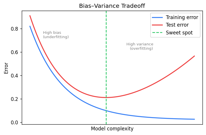
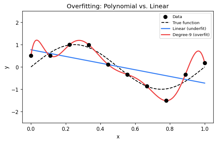
The choice of hypothesis class is critical. If we restrict ourselves to linear functions when the true relationship is nonlinear, no amount of data will save us. If we use a model that is too flexible, we risk fitting noise rather than signal. This tension is formalised by the bias-variance tradeoff.

The Bias-Variance Tradeoff

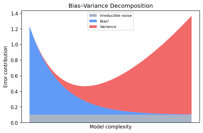
Suppose the true relationship between inputs and outputs is \ + \epsilon), where \ is noise with mean zero. We train a model \ on a finite sample. For a given test point , the expected prediction error decomposes as:

\[ \mathbb{E}[ - y)^2] = \underbrace{\bigl] - f\bigr)^2}_{\text{bias}^2} + \underbrace{\mathbb{E}\bigl[ - \mathbb{E}[\hat{f}])^2\bigr]}_{\text{variance}} + \underbrace{\mathbb{E}[\epsilon^2]}_{\text{irreducible noise}} \]

The bias measures how far the average prediction is from the truth. A model with high bias is too simple; it underfits. The variance measures how much the predictions fluctuate across different training sets. A model with high variance is too complex; it overfits. The irreducible noise is a property of the problem itself and cannot be reduced by any model.

Much of machine learning is about navigating this tradeoff. Regularisation, cross-validation, and careful model selection are all tools for finding the sweet spot where the sum of squared bias and variance is minimised.

Why Machine Learning Matters

Machine learning is no longer a niche academic pursuit. It powers web search, recommendation engines, autonomous vehicles, drug discovery, protein structure prediction, and countless other applications. The explosive growth of data and compute has made previously intractable problems solvable. Every student of computer science should understand the fundamental algorithms that underpin this revolution — not because these exact algorithms are always deployed in production, but because they provide the conceptual vocabulary for understanding, designing, and evaluating more advanced methods.

---

Chapter 2: K-Nearest Neighbours

The Idea Behind KNN

Suppose you want to classify a new data point but you have no parametric model of the data. The simplest strategy is to look at the training examples that are most similar to the query and let them vote. This is the essence of the -nearest neighbours algorithm: to predict the label of a test point , find the \ training points closest to \ and return the majority label or the average target value.

KNN is a non-parametric method. Unlike linear regression or logistic regression, it does not learn a fixed-size parameter vector . Instead, it stores the entire training set and computes predictions on the fly. This makes training trivial — there is nothing to learn — but prediction expensive, since every query requires scanning the dataset.

Distance Metrics

The notion of “closest” depends on the choice of distance metric. The most common choices for \ are:

Metric	Formula	Properties
Euclidean)	^2})	Rotation invariant, most common
Manhattan)	\	Robust to outliers in single coordinates
Minkowski)	^{1/p})	Generalises both; \ is max metric

The choice of metric can dramatically affect performance. In practice, features are often normalised so that no single dimension dominates the distance computation.

The KNN Algorithm

For classification with \ neighbours, the algorithm is:

1. Given a test point , compute the distance from \ to every training point .
2. Select the \ training points with the smallest distances. Call this set \).
3. Return the majority vote: } \mathbf{1}[y_i = c]).

For regression, step 3 is replaced by returning the average: } y_i).

The implicit assumption is that if two feature vectors \ and \ are close, their labels \ and \ are likely the same. This is a form of smoothness assumption on the underlying data distribution.

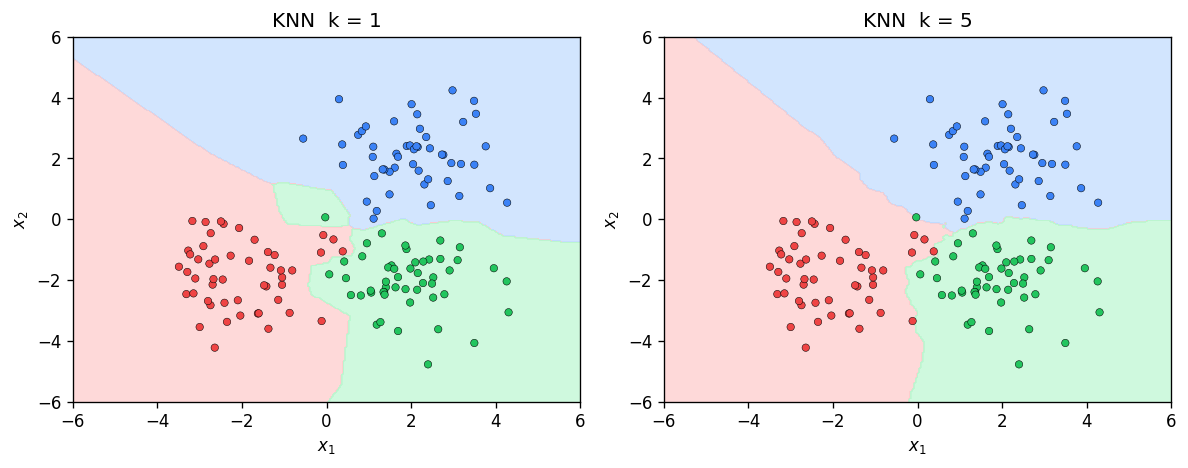
The Role of \

The hyperparameter \ controls the complexity of the model. When , the decision boundary is extremely jagged: every training point creates its own Voronoi cell, and the model memorises the training set exactly. This corresponds to high variance and low bias. As \ increases, the decision boundary becomes smoother. In the extreme case , the classifier always predicts the majority class in the entire training set — high bias, zero variance.

Choosing \ well is critical. A standard approach is to use cross-validation: split the training data into folds, evaluate different values of , and select the one that minimises validation error.

The Bayes Classifier and the Cover-Hart Theorem

To understand the theoretical properties of KNN, we need the concept of the Bayes optimal classifier. Given the true data distribution , the Bayes classifier predicts:

\[ f^* = \arg\max_c \Pr \]

No classifier can achieve lower error than the Bayes classifier. The Bayes error \ is the error rate of this optimal classifier.

This is a remarkable result: with enough data, the simplest possible classifier — just copy the label of the nearest neighbour — achieves an error rate within a factor of two of the best possible. For the general -NN classifier, as both \ and , the error converges to the Bayes error.

The Curse of Dimensionality

The Cover-Hart guarantee is asymptotic: it requires . In practice, when the dimension \ is large, we may need an exponentially large number of training points to fill the space densely enough for nearest neighbours to be meaningful. This phenomenon is the curse of dimensionality.

In high dimensions, distances between points concentrate: the ratio of the distance to the nearest neighbour to the distance to the farthest neighbour approaches 1. When all points are roughly equidistant, the notion of “nearest” becomes meaningless. This is why KNN often performs poorly on raw high-dimensional data without dimensionality reduction.

Computational Considerations

Naively, classifying a single test point requires computing \ distances, each costing \), for a total of \) per query. Storing the entire dataset requires \) space. For large datasets, this is prohibitive.

Several data structures can accelerate nearest-neighbour queries. KD-trees partition the feature space along coordinate axes, enabling average-case \) queries in low dimensions. However, their performance degrades to \) as \ grows. Ball trees and locality-sensitive hashing offer alternatives that trade exactness for speed, providing approximate nearest neighbours in sublinear time.

---

Chapter 3: Linear Regression

Setting Up the Problem

Linear regression is the workhorse of supervised learning for continuous-valued outputs. We are given a training set \}_{i=1}^n) where each \ is a feature vector and \ is a scalar target. The goal is to find a linear function that maps inputs to outputs:

\[ \hat{y} = h = w_0 + w_1 x_1 + w_2 x_2 + \cdots + w_d x_d = \mathbf{w}^\top \bar{\mathbf{x}} \]

where ^\top) includes a constant 1 for the bias term , and ^\top). This padding trick lets us absorb the bias into the weight vector and write the prediction compactly as an inner product.

The assumption that the hypothesis is linear may seem restrictive, but it serves as a fundamental building block. Many powerful methods — polynomial regression, kernel methods, neural networks — generalise linear regression in various ways.

Ordinary Least Squares

To find the best linear function, we minimise the sum of squared errors:

\[ L = \sum_{i=1}^n^2 = \|\mathbf{y} - \bar{X}^\top \mathbf{w}\|_2^2 \]

where \ \times n}) is the matrix whose columns are the padded feature vectors , and ^\top).

Expanding and taking the gradient:

\[ \nabla_{\mathbf{w}} L = -2\bar{X} \]

Setting this to zero yields the normal equations . If \ is invertible, the closed-form solution is:

The matrix \ is always positive semidefinite: for any , we have . This confirms that the loss function is convex, and any critical point is a global minimum.

Gradient Descent for Linear Regression

When \ and \ are large, computing and inverting \ can be expensive. An alternative is gradient descent, which iteratively updates the weights:

\[ \mathbf{w}_{t+1} = \mathbf{w}_t - \eta \nabla_{\mathbf{w}} L \]

where \ is the learning rate. For linear regression with the squared loss:

\[ \nabla_{\mathbf{w}} L = 2A^\top \]

Each gradient step costs \), which is cheaper than the \) cost of the closed-form solution when we only need a few iterations. Stochastic gradient descent further reduces the per-step cost by computing the gradient on a random subset of the data.

Since the squared loss is convex, gradient descent with a sufficiently small step size is guaranteed to converge to the global minimum. The convergence rate depends on the condition number of : the ratio of its largest to smallest eigenvalue. Ill-conditioned problems converge slowly; this is where regularisation and preconditioning help.

Regularisation: Ridge and Lasso

With many features and limited data, the OLS solution can overfit. Small changes in the training data lead to large changes in , producing predictions with high variance. Regularisation controls this by adding a penalty on the complexity of .

Ridge regression regularisation) adds a penalty proportional to :

\[ L_{\text{ridge}} = \|A\mathbf{w} - \mathbf{y}\|_2^2 + \lambda \|\mathbf{w}\|_2^2 \]

The closed-form solution is ^{-1}A^\top \mathbf{y}). The regularisation parameter \ shrinks the weights towards zero and ensures invertibility even when \ is singular. Geometrically, the penalty constrains \ to lie within a ball centred at the origin.

Lasso regression regularisation) uses the penalty :

\[ L_{\text{lasso}} = \|A\mathbf{w} - \mathbf{y}\|_2^2 + \lambda \|\mathbf{w}\|_1 \]

The Lasso produces sparse solutions: many components of \ are exactly zero, effectively performing feature selection. There is no closed-form solution; iterative methods such as coordinate descent are used instead.

Method	Penalty	Sparsity	Closed form?
OLS	None	No	Yes
Ridge	\	No	Yes
Lasso	\	Yes	No

The Statistical Perspective: Maximum Likelihood

Linear regression can be motivated from a probabilistic viewpoint. Suppose the data is generated by a linear model corrupted by Gaussian noise:

\[ y = \mathbf{w}^\top \mathbf{x} + \epsilon, \qquad \epsilon \sim \mathcal{N} \]

Then the conditional distribution of \ given \ is:

\[ p = \frac{1}{\sqrt{2\pi\sigma^2}} \exp\!\left^2}{2\sigma^2}\right) \]

The likelihood of the entire dataset, assuming the data points are independent, is:

\[ L = \prod_{i=1}^n p \]

Maximising the log-likelihood is equivalent to minimising the negative log-likelihood. Dropping constants that do not depend on :

\[ -\log L = \frac{1}{2\sigma^2}\sum_{i=1}^n^2 + \text{const} \]

This is precisely the sum of squared errors! The maximum likelihood estimate under Gaussian noise coincides with the ordinary least squares solution. This beautiful connection tells us that choosing the squared loss is not arbitrary — it is the principled choice when the noise is Gaussian.

Maximum A Posteriori and Regularisation

If we place a prior distribution on , Bayes’ theorem gives the posterior:

\[ p \propto p \cdot p \]

The MAP estimate maximises this posterior. With a Gaussian prior \), the MAP objective becomes:

\[ \min_{\mathbf{w}} \sum_{i=1}^n^2 + \frac{\sigma^2}{\tau^2}\|\mathbf{w}\|_2^2 \]

This is exactly ridge regression with . Similarly, a Laplace prior on \ leads to the Lasso penalty. The statistical perspective thus provides a principled justification for regularisation: it encodes our prior belief about the plausible magnitude of the weights.

Cross-Validation for Model Selection

The regularisation parameter \ must be chosen carefully. Too small and we overfit; too large and we underfit. Cross-validation is the standard technique.

In -fold cross-validation, the training set is partitioned into \ roughly equal folds. For each candidate value of , we train on \ folds and evaluate on the held-out fold, rotating through all folds. The \ with the lowest average validation error is selected. Common choices are \ or ; the special case \ is called leave-one-out cross-validation.

The Bias-Variance Decomposition for Regression

Returning to the bias-variance tradeoff with the notation of Yu’s notes, the regression function \ = \mathbb{E}[Y \mid X = \mathbf{x}]) is the optimal predictor under squared loss. No function \ can reduce the term \|^2]), which represents the intrinsic difficulty of the problem. When we restrict to a function class , we introduce approximation error. Using a finite training set introduces estimation error. Linear regression with a small number of features has low variance but potentially high bias; adding polynomial features reduces bias at the cost of higher variance.

---

Chapter 4: Statistical Learning Theory

The Challenge of Generalisation

Every machine learning algorithm faces the same fundamental question: will it perform well on data it has never seen? Training error alone tells us nothing about generalisation. A model that memorises the training set achieves zero training error but may fail catastrophically on new data. Statistical learning theory provides the mathematical framework for understanding when and why learning from finite data is possible.

The PAC Learning Framework

The Probably Approximately Correct framework, introduced by Leslie Valiant in 1984, formalises the idea that a learning algorithm should, with high probability, output a hypothesis that is approximately correct.

The key point is that the sample complexity must be polynomial in \ and . The framework captures the idea that we want to be “probably”) “approximately”) correct.

Empirical Risk Minimisation

In practice, we do not know the true data distribution . Instead, we observe a training set drawn i.i.d. from \ and minimise the empirical risk:

\[ \hat{R} = \frac{1}{n}\sum_{i=1}^n \ell, y_i) \]

where \ is a loss function. This approach is called empirical risk minimisation. The hope is that for large , the empirical risk is close to the true risk \ = \mathbb{E}_{ \sim P}[\ell, y)]) uniformly over the hypothesis class.

Concentration Inequalities

The bridge between empirical and true risk is provided by concentration inequalities. The most fundamental is:

For a single, fixed hypothesis , Hoeffding’s inequality tells us that \) concentrates around \) at a rate of \). But ERM searches over a hypothesis class , and we need a uniform guarantee over all .

The Union Bound Argument

For a finite hypothesis class , we can apply the union bound:

\[ \Pr\!\left - R| \geq t\right) \leq \sum_{h \in \mathcal{H}} \Pr - R| \geq t) \leq 2M \exp\!\left \]

Setting the right-hand side equal to \ and solving for , we find that with probability at least :

\[ \sup_{h \in \mathcal{H}} |\hat{R} - R| \leq \sqrt{\frac{\log}{2n}} \]

This means the sample complexity for uniform convergence is \). The dependence on \ itself) is crucial: it means that even exponentially large hypothesis classes can be learnable if their “effective size” is controlled.

VC Dimension

For infinite hypothesis classes), the union bound over a finite class does not directly apply. The Vapnik-Chervonenkis dimension provides the right notion of complexity.

For example, the class of linear classifiers in \ has VC dimension . Three non-collinear points in \ can be shattered by lines, but no set of four points can be.

The VC dimension replaces \ in the generalisation bound. Specifically, the fundamental theorem of statistical learning states that a hypothesis class is PAC-learnable if and only if its VC dimension is finite. The sample complexity scales as:

\[ n = O\!\left + \log}{\epsilon^2}\right) \]

Structural Risk Minimisation

The bias-variance tradeoff from Chapter 1 has a precise analogue in learning theory. Consider a sequence of nested hypothesis classes \ with increasing VC dimension. For each class, we can bound the true risk:

\[ R \leq \hat{R} + \text{complexity penalty}, n, \delta) \]

Structural risk minimisation selects the hypothesis class \ that minimises this bound. Using a richer class reduces the empirical risk but increases the complexity penalty. SRM provides a principled way to balance these competing effects without needing a separate validation set.

---

Chapter 5: Logistic Regression and Generalised Linear Models

From Regression to Classification

In the previous chapters, linear regression addressed continuous outputs. But many real-world problems require predicting discrete labels. Can we adapt the linear framework for classification?

A naive approach is to use linear regression with labels \ and threshold the output: predict class 1 if . This works poorly because the linear function is unbounded, so we may get predictions far outside , and the squared loss treats all errors equally rather than penalising confident wrong predictions more. As Yu’s notes observe, reducing classification to regression solves a harder problem than necessary.

What we really want is a model that outputs a probability \ = \Pr \in [0, 1]). This probability should depend on the features through a linear combination , but mapped into .

The Sigmoid Function and Log-Odds

The key insight is to model the log-odds as a linear function:

\[ \log \frac{p}{1 - p} = \mathbf{w}^\top \mathbf{x} \]

The left-hand side ranges over all of , matching the range of the linear function on the right. Solving for \ gives:

The sigmoid function is an S-shaped curve that maps \ to \). It satisfies the useful identity \ = 1 - \sigma), and its derivative is \ = \sigma)).

Prediction is straightforward: predict class 1 if \ > 1/2), equivalently if . This is the same decision rule as the perceptron! The difference is that logistic regression also provides calibrated probability estimates and uses a different training objective.

Maximum Likelihood Estimation

We model the data with a Bernoulli distribution: \ = p^{y})^{1 - y}) for . Given an i.i.d. training set, the conditional log-likelihood is:

\[ \ell = \sum_{i=1}^n \bigl[y_i \log p +\log)\bigr] \]

Maximising this is equivalent to minimising the cross-entropy loss:

\[ L = -\ell = \sum_{i=1}^n \bigl[-y_i \log p_i -\log\bigr] \]

Using the \ encoding for labels, the loss takes the elegant form:

\[ L = \sum_{i=1}^n \log\bigl\bigr) \]

where . This is the sum of the logistic loss \ = \log) evaluated at the “margin” . When the margin is large and positive, the loss is near zero. When it is negative, the loss grows linearly.

Convexity and Optimisation

A crucial property of the cross-entropy loss is that it is convex in . This can be verified by computing the Hessian. The gradient of the loss labels) is:

\[ \nabla_{\mathbf{w}} \ell_i = - y_i)\,\mathbf{x}_i \]

and the Hessian contribution is:

\[ H_i = p_i\,\mathbf{x}_i \mathbf{x}_i^\top \]

Since \ > 0), each \ is positive semidefinite, confirming convexity.

Unlike linear regression, there is no closed-form solution. We must resort to iterative methods:

Gradient descent updates \mathbf{x}_i). A safe step size is , where \ is the spectral norm of the data matrix. Stochastic gradient descent uses mini-batches for efficiency.

Newton’s method uses second-order information: , where \mathbf{x}_i\mathbf{x}_i^\top). This converges quadratically near the optimum but requires \) memory and \) per step for the matrix inversion.

Multiclass Logistic Regression: The Softmax

For \ classes, we generalise the sigmoid to the softmax function. Each class \ has its own weight vector , and:

\[ \Pr = \frac{\exp}{\sum_{\ell=1}^c \exp} \]

This is known as multinomial logistic regression or softmax regression. The loss function becomes the multiclass cross-entropy, and the optimisation is again convex.

Generalised Linear Models and the Exponential Family

Logistic regression is a special case of the broader framework of generalised linear models. The key observation, as Poupart emphasises in his lectures, is that when the class-conditional distributions belong to the exponential family, the posterior probability takes the form of a sigmoid or softmax that is linear in .

The Gaussian, Bernoulli, Poisson, gamma, and many other common distributions are members of the exponential family. When we use a categorical prior over classes and exponential family class-conditionals, Bayes’ theorem yields a posterior that is precisely a softmax of linear functions. Logistic regression directly parametrises this posterior, bypassing the need to estimate the class-conditional distributions. This is the distinction between generative models and discriminative models) directly).

---

Chapter 6: The Perceptron

Historical Context

The perceptron, introduced by Frank Rosenblatt in 1958, was the first algorithmically defined learning machine and one of the foundational results of artificial intelligence. Inspired by biological neurons, the perceptron receives a weighted sum of inputs, applies a threshold, and outputs a binary decision. Despite its simplicity, the perceptron carries deep lessons about linear classifiers, convergence guarantees, and the limits of single-layer models.

The Perceptron Model

Using the padding trick into \ and appending a 1 to ), we can write the prediction as \) where \ and \ are now \)-dimensional.

The Perceptron Algorithm

The perceptron is an online algorithm: it processes training examples one at a time and updates only when it makes a mistake.

Algorithm:

1. Initialise .
2. For each training example \):
   • Compute \).
   • If \ \leq 0)):
     • Update: .
3. Repeat until no mistakes are made on a full pass through the data.

The update rule has an elegant geometric interpretation. When the perceptron misclassifies a positive example), adding \ to \ rotates the weight vector towards , increasing the inner product \ and making a correct classification more likely next time. Conversely, for a misclassified negative example, subtracting \ rotates \ away from .

As Yu’s notes observe, the key insight is that after an update, . The update strictly improves the margin on the misclassified point — and the remarkable fact is that it does not ruin the possibility of satisfying all other constraints.

Linear Separability and the Geometric Margin

A large margin means the classes are well-separated and classification is “easy.” A small margin means the classes are nearly overlapping and classification is difficult.

The Perceptron Convergence Theorem

The most important theoretical result about the perceptron is its finite convergence guarantee.

Proof sketch. We track two quantities across the sequence of updates. After \ mistakes:

Lower bound on growth of : Each update increases the inner product with the reference solution by at least :

\[ \langle \mathbf{w}_{k+1}, \mathbf{w}^*\rangle = \langle \mathbf{w}_k, \mathbf{w}^*\rangle + \langle \mathbf{a}, \mathbf{w}^*\rangle \geq \langle \mathbf{w}_k, \mathbf{w}^*\rangle + s \]

By telescoping: .

Upper bound on growth of : Each update increases the squared norm by at most ):

\[ \|\mathbf{w}_{k+1}\|_2^2 = \|\mathbf{w}_k\|_2^2 + 2\langle \mathbf{w}_k, \mathbf{a}\rangle + \|\mathbf{a}\|_2^2 \leq \|\mathbf{w}_k\|_2^2 + R^2 \]

By telescoping: .

Combining: By Cauchy-Schwarz, . Squaring both sides: , giving . \

The bound is tightest when we optimise over the choice of reference solution . Since both \ and \ scale together if we rescale , we can normalise to , in which case the bound becomes , where \ is the geometric margin.

Limitations: The XOR Problem

The perceptron can only learn linearly separable functions. The classic counterexample is the XOR function: \ \to -1), \ \to +1), \ \to +1), \ \to -1). No single hyperplane can separate the positive and negative examples. When presented with linearly inseparable data, the perceptron will cycle endlessly through the training set, never converging.

This limitation was famously highlighted by Minsky and Papert in 1969, leading to a prolonged “AI winter” during which interest in neural networks waned. The resolution came decades later with the development of multi-layer networks and the backpropagation algorithm, which can represent nonlinear decision boundaries.

Connections to SVMs and Neural Networks

The perceptron’s convergence bound \ reveals that the margin is the key geometric quantity. Support vector machines take this insight to its logical conclusion: instead of finding any separating hyperplane, they find the one that maximises the margin. The perceptron can be viewed as a stochastic approximation to the SVM objective.

Similarly, the perceptron is a single-layer neural network with a sign activation function. By stacking multiple layers of perceptron-like units with differentiable activation functions, we obtain multi-layer perceptrons that can represent arbitrarily complex decision boundaries — overcoming the XOR limitation.

---

Chapter 7: Mixture Models and the EM Algorithm

Unsupervised Learning and Clustering

So far, every algorithm we have studied has relied on labelled data: pairs \) where the correct output is known. In many settings, labels are expensive or unavailable, and we must discover structure in the data without supervision. Clustering is the canonical unsupervised learning problem: given points , partition them into groups such that points within a group are similar and points across groups are dissimilar.

-Means Clustering

The -means algorithm is the simplest and most widely used clustering method. It seeks to partition \ points into \ clusters \ by minimising the total within-cluster variance:

\[ \min_{C_1, \ldots, C_k} \sum_{j=1}^k \sum_{\mathbf{x}_i \in C_j} \|\mathbf{x}_i - \boldsymbol{\mu}_j\|_2^2, \qquad \boldsymbol{\mu}_j = \frac{1}{|C_j|}\sum_{\mathbf{x}_i \in C_j} \mathbf{x}_i \]

where \ is the centroid of cluster .

Lloyd’s algorithm is the standard heuristic for -means. It alternates between two steps:

1. Assignment step: Assign each point to the cluster with the nearest centroid: .
2. Update step: Recompute each centroid as the mean of its assigned points.

These steps are repeated until convergence. Each step decreases or maintains the objective, so the algorithm is guaranteed to converge, though only to a local minimum. The -means problem is NP-hard in general, even to approximate within a constant factor, so multiple random restarts are standard practice.

From Hard Clustering to Soft Clustering

-means assigns each point to exactly one cluster — a “hard” assignment. But what if a point lies between two clusters? It may be more natural to say that the point belongs 60% to cluster 1 and 40% to cluster 2. This motivates a probabilistic approach where cluster membership is represented by a probability distribution.

Gaussian Mixture Models

A Gaussian mixture model assumes that the data is generated by a mixture of \ Gaussian distributions:

\[ p = \sum_{j=1}^k \pi_j \,\mathcal{N} \]

where \ are the mixing weights), and each component is a multivariate Gaussian with mean \ and covariance . The parameters are \}_{j=1}^k).

The generative story is: to produce a data point, first sample a component \), then sample \). The latent variable \ tells us which component generated the point, but it is unobserved.

If we knew the latent assignments , estimation would be straightforward: for each component, compute the empirical mean, covariance, and proportion from the assigned points. The difficulty is that we do not know the assignments, and directly maximising the log-likelihood

\[ \ell = \sum_{i=1}^n \log \sum_{j=1}^k \pi_j \,\mathcal{N} \]

is intractable because the log of a sum does not simplify nicely.

The EM Algorithm

The Expectation-Maximisation algorithm, introduced by Dempster, Laird, and Rubin, is a general technique for maximum likelihood estimation in the presence of latent variables. Applied to GMMs, it alternates between computing soft assignments and updating the parameters.

The derivation begins with a lower bound on the log-likelihood. For any distributions \ over the latent variable , Jensen’s inequality gives:

\[ \log p = \log \sum_j q_i \frac{p}{q_i} \geq \sum_j q_i \log \frac{p}{q_i} \]

This lower bound is tight when \ = p), the posterior distribution of the latent variable. EM alternates between maximising the ELBO over \ and over .

E-step: Fix . For each data point \ and each component , compute the responsibility:

\[ r_{ij} = q_i = \frac{\pi_j \,\mathcal{N}}{\sum_{\ell=1}^k \pi_\ell \,\mathcal{N}} \]

This is the posterior probability that point \ was generated by component . It is the “soft assignment” analogue of -means’ hard assignment.

M-step: Fix the responsibilities . Update the parameters using weighted statistics:

\[ n_j = \sum_{i=1}^n r_{ij}, \qquad \boldsymbol{\mu}_j = \frac{1}{n_j}\sum_{i=1}^n r_{ij}\,\mathbf{x}_i, \qquad \Sigma_j = \frac{1}{n_j}\sum_{i=1}^n r_{ij}^\top, \qquad \pi_j = \frac{n_j}{n} \]

These are simply the weighted mean, covariance, and proportion, where the weights are the responsibilities.

Convergence Properties

Each iteration of EM is guaranteed to increase the log-likelihood:

\[ \ell}) \geq \ell}) \]

This follows from the fact that the E-step makes the lower bound tight, and the M-step increases the lower bound. Since the log-likelihood is bounded above, the sequence converges. However, like -means, EM converges only to a local maximum of the likelihood, not necessarily the global maximum. Multiple random initialisations are recommended.

-Means as a Special Case of EM

There is a beautiful connection between -means and EM. Consider a GMM where all covariance matrices are \ and we take the limit . In this limit, the responsibilities become “hard”: \ for the closest centroid and 0 for all others. The E-step reduces to the assignment step of -means, and the M-step reduces to recomputing the centroids. Thus, -means is a “hard” version of EM for spherical Gaussians with vanishing variance.

Model Selection: How Many Components?

Choosing the number of components \ is a model selection problem. Simply maximising the likelihood does not work: adding more components always increases the likelihood. We need a criterion that penalises model complexity.

The Bayesian Information Criterion and Akaike Information Criterion are two widely used approaches:

\[ \text{BIC} = -2\ell + p \log n, \qquad \text{AIC} = -2\ell + 2p \]

where \ is the number of free parameters and \ is the MLE. Both criteria balance goodness of fit against complexity. BIC imposes a heavier penalty for large \ and tends to select simpler models; AIC is better suited when the goal is prediction rather than model identification. In practice, one fits GMMs for \ and selects the \ that minimises BIC or AIC.

Another approach is to use cross-validation, holding out data and evaluating the log-likelihood on the held-out set. This is more computationally expensive but avoids the assumptions built into BIC and AIC.

Beyond Gaussians

The EM framework is not limited to Gaussian components. Any mixture model with tractable E-step and M-step computations can be fit using EM. Mixtures of Bernoullis, mixtures of multinomials, and mixtures of other exponential family distributions are all common in practice. The general principle remains the same: introduce latent variables, compute posterior responsibilities in the E-step, and update parameters in the M-step.

Chapter 8: Support Vector Machines

Support vector machines occupied the throne of machine learning for nearly two decades before deep neural networks took over around 2010. In the low-data regime they remain remarkably effective, and the mathematical framework they rest on — maximum-margin separation, Lagrangian duality, and the kernel trick — continues to inform modern algorithm design. This chapter develops the theory from first principles.

The Maximum-Margin Classifier

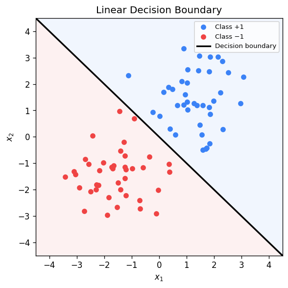
Consider a binary classification problem with a training set \ \subseteq \mathbb{R}^d \times {+1,-1} : i=1,\dots,n}). When the data are linearly separable, there exists a hyperplane \ such that every training point is correctly classified:

\[ \forall\, i,\quad y_i > 0. \]

Infinitely many such hyperplanes exist — perturbing \) slightly preserves the separation. The perceptron algorithm finds any separating hyperplane. SVMs ask a sharper question: among all separating hyperplanes, which one is optimal?

The distance from a point \ to the hyperplane \ equals . When the hyperplane correctly classifies \), the signed quantity \ / |\mathbf{w}|_2) is positive and equals the geometric distance. The SVM seeks to maximize this worst-case distance:

\[ \max_{\mathbf{w},b} \min_{i=1,\dots,n} \frac{y_i}{\|\mathbf{w}\|_2}. \]

This formulation is scale-invariant: replacing \) by \) for any \ does not change the hyperplane or the objective. We exploit this freedom by fixing the minimum functional margin to be 1, that is, requiring \ = 1). Under this normalization the margin becomes , and maximizing it is equivalent to minimizing . We arrive at the hard-margin SVM:

\[ \min_{\mathbf{w}, b} \; \frac{1}{2}\|\mathbf{w}\|_2^2 \quad \text{subject to} \quad y_i \ge 1, \;\; \forall\, i=1,\dots,n. \]

This is a quadratic program: a quadratic objective with linear constraints. In contrast, the perceptron solves a linear feasibility problem with objective identically zero. The SVM objective yields a unique solution, whereas the perceptron admits infinitely many.

Geometry: Three Parallel Hyperplanes and Support Vectors

At the optimum, the constraints partition into active) and inactive). The active constraints correspond to points lying exactly on one of two bounding hyperplanes:

\[ H_+ = \{\mathbf{x} : \langle \mathbf{x}, \mathbf{w} \rangle + b = +1\}, \qquad H_- = \{\mathbf{x} : \langle \mathbf{x}, \mathbf{w} \rangle + b = -1\}. \]

The decision boundary \ lies equidistant between \ and . The strip between \ and \ is a “dead zone” containing no training points. Each bounding hyperplane has distance \ from , so the total margin width is .

At optimality there must be at least one support vector from each class. This sparsity property is what makes SVMs attractive: the decision boundary depends on only a handful of critical training examples.

The Lagrangian Dual Formulation

To solve the constrained QP, we introduce Lagrange multipliers , one per constraint:

\[ \mathcal{L} = \frac{1}{2}\|\mathbf{w}\|_2^2 - \sum_{i=1}^n \alpha_i \bigl[y_i - 1\bigr]. \]

The primal problem is . By strong duality, we can swap the min and max. We first minimize over \ and \ by setting partial derivatives to zero:

\[ \frac{\partial \mathcal{L}}{\partial \mathbf{w}} = \mathbf{w} - \sum_{i=1}^n \alpha_i y_i \mathbf{x}_i = 0 \quad \Longrightarrow \quad \mathbf{w} = \sum_{i=1}^n \alpha_i y_i \mathbf{x}_i, \]\[ \frac{\partial \mathcal{L}}{\partial b} = -\sum_{i=1}^n \alpha_i y_i = 0. \]

Substituting back yields the dual problem:

\[ \max_{\boldsymbol{\alpha} \ge 0} \sum_{i=1}^n \alpha_i - \frac{1}{2}\sum_{i,j} \alpha_i \alpha_j y_i y_j \langle \mathbf{x}_i, \mathbf{x}_j \rangle \quad \text{subject to} \quad \sum_{i=1}^n \alpha_i y_i = 0. \]

Several observations are crucial. First, the dual depends on the data only through inner products \ — this will enable the kernel trick in the next chapter. Second, the KKT complementary slackness conditions require \ - 1] = 0) for all . Thus \ only for support vectors, confirming sparsity.

The weight vector \ is a linear combination of support vectors. At test time, prediction is \ = \text{sign}\bigl), again involving only inner products. The bias \ is recovered from any support vector: \ for any \ with .

The Dual Geometric View

There is an elegant geometric interpretation due to Rosen. A dataset is linearly separable if and only if the convex hulls of the positive and negative examples are disjoint: \ \cap \text{conv} = \emptyset). The SVM hyperplane is the perpendicular bisector of the shortest line segment connecting \) to \). This minimum-distance pair \) may involve convex combinations of training points, not necessarily individual data points. The maximum margin equals half the distance between the two convex hulls.

Soft-Margin SVM

Real datasets are rarely perfectly separable. The soft-margin SVM relaxes the hard constraints by introducing slack variables :

\[ \min_{\mathbf{w}, b, \boldsymbol{\xi}} \; \frac{1}{2}\|\mathbf{w}\|_2^2 + C \sum_{i=1}^n \xi_i \quad \text{subject to} \quad y_i \ge 1 - \xi_i, \;\; \xi_i \ge 0. \]

The hyperparameter \ controls the trade-off between maximizing the margin small) and minimizing training errors small). When , we recover the hard-margin SVM. When , we ignore the data entirely.

The dual of the soft-margin SVM is:

\[ \max_{0 \le \alpha_i \le C} \sum_{i=1}^n \alpha_i - \frac{1}{2}\sum_{i,j} \alpha_i \alpha_j y_i y_j \langle \mathbf{x}_i, \mathbf{x}_j \rangle \quad \text{subject to} \quad \sum_{i=1}^n \alpha_i y_i = 0. \]

The only difference from the hard-margin dual is the box constraint . Complementary slackness now yields a richer structure: if , the point lies on the correct side of the margin; if , the point sits exactly on the margin boundary; if , the point is within the margin or misclassified.

The Hinge Loss Perspective

The soft-margin SVM admits an equivalent unconstrained formulation:

\[ \min_{\mathbf{w}, b} \; \frac{1}{2}\|\mathbf{w}\|_2^2 + C \sum_{i=1}^n_+, \quad \hat{y}_i = \langle \mathbf{x}_i, \mathbf{w} \rangle + b, \]

where _+ = \max{0, t}) is the hinge loss. This loss is zero when the functional margin \ and grows linearly as the margin decreases below 1. The hinge loss is a convex upper bound on the 0-1 loss , and it is classification-calibrated: minimizing it in population leads to the Bayes-optimal classifier. This perspective connects SVMs to empirical risk minimization with regularization. The \ term is the regularizer, and \ plays the role of the inverse regularization strength.

Other surrogate losses lead to different classifiers: the logistic loss \) gives logistic regression, the exponential loss \ leads to AdaBoost, and the squared hinge _+^2) is sometimes preferred for its smoothness.

Optimization

Training an SVM can be done by several methods. The dual QP can be solved by general-purpose QP solvers, but for large-scale problems, specialized algorithms are preferred. The Sequential Minimal Optimization algorithm decomposes the problem into a sequence of two-variable subproblems that admit closed-form solutions. Alternatively, the primal hinge-loss formulation can be optimized directly by stochasticgradient descent: at each step, sample a data point \) and update

\[ \mathbf{w} \leftarrow \mathbf{w} - \eta\biggl, \]

where \). This scales linearly in \ and , making it feasible for very large datasets.

Chapter 9: Kernel Methods

Kernel methods provide a principled framework for extending linear algorithms to handle nonlinear patterns. The central insight is the kernel trick: by replacing inner products with a kernel function, we can implicitly operate in a high-dimensional feature space without ever computing the feature vectors explicitly.

Feature Maps and the Kernel Trick

Consider the XOR problem: four points in \ that no hyperplane can separate. A quadratic classifier \ = \langle \mathbf{x}, Q\mathbf{x} \rangle + \sqrt{2}\langle \mathbf{x}, \mathbf{p} \rangle + b) can separate them. We can rewrite this as a linear function in a lifted feature space by defining the feature map

\[ \phi = \bigl^\top, \]

so that \ = \langle \phi, \mathbf{w} \rangle) for an appropriate weight vector . The feature map \ is nonlinear, but the classifier is linear in the new space.

The key observation is that inner products in feature space can be computed cheaply:

\[ \langle \phi, \phi \rangle =^2. \]

The right-hand side costs \) to evaluate — the same as computing an inner product in the original space — even though the feature space has dimension 6.

Given a feature map , the kernel is determined. Conversely, given a kernel, there exists a canonical feature map \ = k), where \) is viewed as a function in the reproducing kernel Hilbert space. The reproducing property states \ \rangle_{\mathcal{H}_k} = f) for any .

Mercer’s Theorem and Positive Definite Kernels

Not every function of two arguments is a valid kernel. The characterization is given by the following:

This means \ \ge 0) for all . If equality holds only when , the kernel is strictly positive definite. A kernel can be thought of as a similarity measure that respects the geometry of some feature space.

Common Kernels

Polynomial kernel. \ =^p), where \ and . The corresponding feature space contains all monomials up to degree . Setting \ recovers the linear kernel.

Gaussian kernel. \ = \exp), where \ is the bandwidth parameter. This kernel corresponds to an infinite-dimensional feature space. It is universal: its RKHS is dense in the space of continuous functions over any compact domain.

Laplace kernel. \ = \exp). Like the Gaussian kernel but based on the unsquared distance, producing rougher functions.

Sigmoid kernel. \ = \tanh). Not positive definite for all parameter values, so it must be used with care.

Kernel Calculus

Kernels are closed under several operations, enabling construction of complex kernels from simpler ones. If \ and \ are kernels, then so are: \ for ; ; ; and \ when the limit exists. These closure properties follow directly from the PSD characterization.

The Representer Theorem

The proof uses an orthogonal decomposition: write \ where \ lies in the span of \}). The loss depends only on function values at training points, which depend only on . The regularizer , so setting \ cannot increase the objective.

This theorem justifies the kernel SVM: replacing \ with \) in the dual gives the kernelized soft-margin SVM, which implicitly finds the maximum-margin hyperplane in . At test time, prediction is \ = \sum_i \alpha_i y_i k + b), requiring only kernel evaluations and the support vectors.

Kernel Ridge Regression and Kernel PCA

The kernel trick applies to any algorithm that depends on data only through inner products. Kernel ridge regression replaces the linear prediction \ with \), where ^{-1} \mathbf{y}) and \ is the \ kernel matrix. Kernel PCA computes principal components in feature space by eigendecomposing the centered kernel matrix, enabling nonlinear dimensionality reduction.

Reproducing Kernel Hilbert Spaces

The RKHS \ associated with kernel \ is the unique Hilbert space of functions satisfying the reproducing property. Formally, \ : \mathbf{x} \in \mathcal{X}}}), with inner product , k \rangle_{\mathcal{H}_k} = k). The RKHS norm \ measures the complexity of ; regularizing by this norm in empirical risk minimization controls model complexity. A kernel is universal if its RKHS is dense in \) for compact , meaning it can approximate any continuous function. The Gaussian kernel is universal; the polynomial kernel is not.

Computational Trade-offs

Kernelization shifts the computational bottleneck from the feature dimension to the number of training points. Without kernels, training costs \) and testing \). With kernels, forming the Gram matrix costs \), solving the dual is \), and testing costs \) per new point) where \ is the number of support vectors). This makes kernel methods impractical for very large datasets but powerful when \ is moderate and the feature space is high-dimensional or infinite.

Chapter 10: Gaussian Processes

Gaussian processes provide a Bayesian, nonparametric approach to regression and classification. Where kernel SVMs find a single best function, GPs maintain an entire distribution over functions, enabling principled uncertainty quantification.

From Bayesian Linear Regression to GPs

Recall Bayesian linear regression with features \): we place a prior \), assume \ + \epsilon) with \), and compute the posterior \). This is the weight-space view. Alternatively, we can work directly in function space: since \ = \mathbf{w}^\top \phi) is linear in the Gaussian , the function values at any finite collection of inputs are jointly Gaussian.

The mean function is \ = \mathbb{E}[f] = \phi^\top \mathbb{E}[\mathbf{w}] = 0), and the covariance function is

\[ k = \mathbb{E}[ff] = \frac{1}{\alpha}\phi^\top \phi. \]

This is a kernel! The function-space view replaces a distribution over weight vectors with a distribution over functions, described by the mean and covariance functions.

GP Prior and Posterior

The prior \) encodes our beliefs about the function before seeing data. Given training data \ and targets , with a Gaussian likelihood \ + \epsilon_i), the posterior is also a GP. For a test point , the predictive distribution is Gaussian with

\[ \mu_* = \mathbf{k}_*^\top^{-1} \mathbf{y}, \qquad \sigma_*^2 = k - \mathbf{k}_*^\top^{-1} \mathbf{k}_*, \]

where \) is the training kernel matrix and , \dots, k]^\top). The predictive mean \ interpolates the training data, while the predictive variance \ shrinks near observed points and grows in unobserved regions. At a noiseless training point, : there is no uncertainty where we have observed the function.

Kernel Design

The choice of kernel profoundly shapes the GP’s behavior. The Gaussian kernel \ = \exp) produces smooth, infinitely differentiable sample functions. The exponential kernel \ = \exp) yields rougher, continuous but not differentiable samples — resembling Brownian motion paths. The bandwidth \ controls the correlation length: small \ means rapid variation, large \ means slowly varying functions. Kernel hyperparameters are typically set by maximizing the marginal likelihood \), which integrates out the function and naturally trades off data fit against model complexity.

GP for Regression

The computational bottleneck of GP regression is the inversion of the \ matrix , costing \). This is cubic in the number of training points rather than in the feature dimension, which is the complementary trade-off to the weight-space view where complexity is cubic in the number of features. For the Gaussian kernel with infinite-dimensional features, the weight-space approach is impossible, but the function-space GP computation is well-defined.

Sparse GP approximations reduce the cost to \) where \ is the number of inducing points, making GPs feasible for moderately large datasets.

GP for Classification

For binary classification, the likelihood is Bernoulli: \ = \sigma)) where \ is the logistic function. The posterior \) is no longer Gaussian. The Laplace approximation finds a Gaussian approximation centered at the mode of the posterior, then uses this Gaussian to make predictions. Expectation propagation provides an alternative that is often more accurate.

Relationship to Kernel Methods and Neural Networks

GP regression with a Gaussian likelihood is equivalent to kernel ridge regression: the predictive mean is identical. However, GPs additionally provide uncertainty estimates through the predictive variance. A remarkable connection to neural networks was established by Neal: a single-hidden-layer neural network with i.i.d. random weights, as the width tends to infinity, converges in distribution to a GP. The kernel of this limiting GP depends on the activation function. This equivalence has been extended to deep networks, where the Neural Tangent Kernel describes the training dynamics of infinitely wide networks trained by gradient descent.

Chapter 11: Neural Networks and Backpropagation

We now turn from kernel methods, which use fixed feature maps, to neural networks, which learn the feature map jointly with the linear predictor.

From Perceptron to Multi-Layer Perceptron

The single-layer perceptron computes \), which defines a linear decision boundary. It cannot solve the XOR problem. The multi-layer perceptron stacks linear transformations and nonlinear activations:

\[ \mathbf{z} = U\mathbf{x} + \mathbf{c}, \quad \mathbf{h} = \sigma, \quad \hat{y} = \langle \mathbf{h}, \mathbf{w} \rangle + b, \]

where , , and \ is a nonlinear activation function applied element-wise. The hidden layer \ constitutes a learned representation of the input. For XOR, choosing , , , , and \ correctly classifies all four points.

More generally, a depth-\ MLP computes

\[ \mathbf{h}_0 = \mathbf{x}, \quad \mathbf{h}_k = \sigma \;\text{ for } k=1,\dots,L, \quad \hat{\mathbf{y}} = W_{L+1}\mathbf{h}_L + \mathbf{b}_{L+1}, \]

where \ and . For classification into \ classes, the output is passed through a softmax: \ / \sum_j \exp).

The key difference from kernel methods is that the feature map \ = \mathbf{h}_L) is learned through gradient-based optimization rather than fixed a priori.

The Universal Approximation Theorem

This guarantees that a sufficiently wide two-layer network can approximate any continuous function. The caveat is that the required width may be astronomically large. In practice, deeper networks are more parameter-efficient than very wide shallow ones, which motivates deep learning.

An even stronger result is the Kolmogorov-Arnold representation theorem: any continuous function \ can be written as a finite superposition of continuous univariate functions and addition, matching the structure of a two-hidden-layer network.

Forward Pass

The forward pass evaluates the network layer by layer. Each layer applies a linear transformation followed by a nonlinear activation. For a classification task with cross-entropy loss, the forward pass computes:

1. Hidden representations .
2. Logits .
3. Predicted probabilities \).
4. Loss .

Backpropagation

Training requires computing the gradient of the loss with respect to all parameters. Backpropagation is simply the chain rule applied systematically to the computational graph, combined with dynamic programming to avoid redundant computation.

The reverse-mode differentiation algorithm proceeds as follows. Let \ be the “adjoint” of node . Initialize . Then propagate backwards:

\[ V_i = \sum_{j \in \text{successors}} \frac{\partial f_j}{\partial v_i} \cdot V_j. \]

For a depth-\ MLP, this gives the familiar layer-wise backpropagation:

\[ \frac{\partial \ell}{\partial W_k} = \frac{\partial \mathbf{z}_k}{\partial W_k} \cdot \frac{\partial \ell}{\partial \mathbf{z}_k}, \quad \frac{\partial \ell}{\partial \mathbf{h}_{k-1}} = W_k^\top \frac{\partial \ell}{\partial \mathbf{z}_k}, \quad \frac{\partial \ell}{\partial \mathbf{z}_k} = \text{diag}) \cdot \frac{\partial \ell}{\partial \mathbf{h}_k}. \]

Automatic Differentiation

Backpropagation is a special case of automatic differentiation, which computes exact derivatives of any function expressible as a composition of elementary operations.

For neural networks where , reverse-mode AD computes the full gradient in time proportional to a single forward pass. This is why training neural networks is feasible despite having millions of parameters. The forward mode is preferable when the input dimension \ is small and the output dimension \ is large. Modern deep learning frameworks implement reverse-mode AD automatically.

Activation Functions

The choice of activation function significantly affects training dynamics:

Sigmoid: \ = 1/). Outputs in \), saturates for large , causing vanishing gradients.

Tanh: \ = 2\sigma - 1). Zero-centered, but still saturates.

ReLU: \ = \max). Non-saturating for positive inputs, but “dead” neurons can occur when inputs are always negative. Dominates modern architectures due to computational simplicity and strong gradient signal.

GELU: \ = t \cdot \Phi), where \ is the standard Gaussian CDF. Smooth approximation to ReLU that is differentiable everywhere. Used extensively in Transformers.

Leaky ReLU and ELU address the dead neuron problem by allowing small gradients for negative inputs.

Chapter 12: Training Deep Neural Networks

Building a deep network architecture is only half the challenge; training it effectively requires navigating a complex, non-convex loss landscape. This chapter covers the practical toolkit for training deep networks.

Loss Landscapes and Optimization Challenges

The loss function of a deep network, as a function of its parameters, is highly non-convex with many local minima, saddle points, and flat regions. Despite this, gradient-based optimization works remarkably well in practice. Key challenges include: vanishing or exploding gradients as depth increases; sensitivity to initialization; balancing learning speed with generalization.

Stochastic Gradient Descent and Variants

Full-batch gradient descent computes the gradient over all \ training examples per step:

\[ \boldsymbol{\theta} \leftarrow \boldsymbol{\theta} - \eta \cdot \frac{1}{n}\sum_{i=1}^n \nabla_{\boldsymbol{\theta}} \ell, y_i). \]

Stochastic gradient descent replaces the full sum with a minibatch :

\[ \boldsymbol{\theta} \leftarrow \boldsymbol{\theta} - \eta \cdot \frac{1}{|B|}\sum_{i \in B} \nabla_{\boldsymbol{\theta}} \ell, y_i). \]

The minibatch gradient is an unbiased estimate of the full gradient. Smaller batches introduce more noise but can escape sharp local minima and often lead to better generalization.

Momentum accelerates SGD by accumulating a running average of past gradients:

\[ \mathbf{v}_{t+1} = \beta \mathbf{v}_t + \eta \nabla \ell, \quad \boldsymbol{\theta}_{t+1} = \boldsymbol{\theta}_t - \mathbf{v}_{t+1}. \]

This dampens oscillations and speeds convergence along consistent gradient directions. The coefficient \) controls the “memory” of past gradients.

Nesterov momentum evaluates the gradient at a “look-ahead” position: \), where \). This achieves the optimal \) convergence rate for convex problems.

AdaGrad adapts the learning rate per parameter by dividing by the accumulated sum of squared gradients. It works well for sparse gradients but can prematurely shrink the learning rate.

RMSProp fixes this by using an exponential moving average of squared gradients:

\[ s_t =s_{t-1} + \lambda^2, \quad \boldsymbol{\theta} \leftarrow \boldsymbol{\theta} - \frac{\eta}{\sqrt{s_t + \epsilon}} \odot \nabla \ell. \]

Adam combines momentum with adaptive learning rates:

\[ \mathbf{v}_t =\mathbf{v}_{t-1} + \gamma \nabla \ell, \quad s_t =s_{t-1} + \lambda^2, \]

with bias correction applied to both estimates. Adam is the default optimizer in most deep learning applications, though SGD with momentum can sometimes achieve better generalization with careful tuning.

Learning Rate Schedules

The learning rate \ is perhaps the single most important hyperparameter. Common strategies include:

Step decay: Reduce \ by a factor every fixed number of epochs.

Cosine annealing: )), smoothly decaying from \ to \ over \ iterations.

Warmup: Start with a very small learning rate and linearly increase it over a warmup period before applying the main schedule. Used in Transformer training, where the original Attention Is All You Need paper used \) with warmup steps .

Normalization

Batch normalization normalizes activations across the minibatch. For a layer with activations , BN computes /\sqrt{\sigma_j^2 + \epsilon}) where \ and \ are the minibatch mean and variance of the -th feature. Learnable scale \ and shift \ parameters are applied afterwards: . During testing, running averages of the training statistics are used. BN stabilizes training, allows higher learning rates, and acts as a regularizer.

Layer normalization normalizes across features rather than across the batch, making it suitable for variable-length sequences and small batches. It is the standard in Transformers.

Regularization

Dropout randomly sets each hidden unit to zero with probability \ during training. At test time, no units are dropped, but weights are scaled by \ during training). Dropout prevents co-adaptation of neurons and can be interpreted as an implicit ensemble of exponentially many sub-networks.

Weight decay adds an \ penalty \ to the loss, equivalent to decaying the weights by a factor \) at each SGD step.

Early stopping monitors performance on a validation set and halts training when validation loss begins to increase, preventing overfitting. It can be shown to be equivalent to a form of \ regularization.

Initialization Strategies

Proper initialization is critical to prevent vanishing or exploding signals at the start of training.

Xavier initialization sets weights as )) or uniformly in }, \sqrt{6/}]). This maintains variance of activations across layers for linear or tanh activations.

He initialization uses \), which accounts for the fact that ReLU zeros out roughly half the inputs. This is the standard for networks using ReLU activations.

Chapter 13: Convolutional Neural Networks

Convolutional neural networks exploit the spatial structure of images through three key ideas: local connectivity, weight sharing, and translation equivariance. They have been the dominant architecture for computer vision since AlexNet’s breakthrough on ImageNet in 2012.

The Convolution Operation

In an MLP, each output neuron connects to every input. For images, this is wasteful: a pixel’s neighbors carry far more information than distant pixels. A convolutional layer restricts connections to a local window and slides it across the input:

\[ _{ij} = \sigma\Bigl_{i+a, j+b, c} + \text{bias}\Bigr), \]

where \ is a filter of spatial size \ and depth . The same weights are applied at every spatial position — this is weight sharing. Multiple filters produce multiple output feature maps, each detecting a different pattern.

The output spatial dimensions are determined by the input size, filter size, stride, and padding. For input size , filter , stride , and padding :

\[ \text{output size} = \left\lfloor\frac{m + 2p - a}{s}\right\rfloor + 1 \quad \times \quad \left\lfloor\frac{n + 2q - b}{t}\right\rfloor + 1. \]

Pooling Layers

Pooling reduces spatial resolution, decreasing computation and providing some translation invariance. Max pooling takes the maximum value in each local window; average pooling takes the mean. Pooling operates independently on each channel and has no learnable parameters. Global average pooling reduces each feature map to a single value by averaging over the entire spatial extent, often used before the final classification layer.

Architecture Evolution

The evolution of CNN architectures illustrates key design principles:

LeNet was among the first successful CNNs, applied to handwritten digit recognition. It uses two convolutional layers with average pooling, followed by fully connected layers.

AlexNet scaled up to 8 layers and won the ImageNet Large Scale Visual Recognition Challenge by a wide margin. Key innovations included ReLU activations, dropout regularization, and GPU training.

VGGNet demonstrated that depth matters: using only \ filters, it achieved excellent results with 16–19 layers. Three stacked \ filters have the same receptive field as one \ filter but with fewer parameters: \ = 27) versus \).

GoogLeNet/Inception introduced the Inception module with parallel branches of different filter sizes, and notably used \ convolutions to control channel dimensionality. It was deeper yet more efficient, eliminating fully connected layers in favor of global average pooling.

Skip Connections and Residual Learning

ResNet solved the degradation problem — deeper networks can paradoxically perform worse than shallower ones — by introducing skip connections. A residual block computes

\[ \mathbf{h}_{l+1} = \sigma), \]

where \ is a stack of convolutional layers. The network only needs to learn the residual \ rather than the full mapping. Skip connections provide a direct path for gradients during backpropagation, enabling training of networks with over 100 layers. If the optimal transformation is close to the identity, learning a small residual is far easier than learning the full function from scratch.

Transfer Learning and Fine-Tuning

Training a CNN from scratch requires large datasets and significant compute. Transfer learning leverages a network pre-trained on a large dataset and adapts it to a new task. In feature extraction, the pre-trained convolutional layers are frozen and only the final classifier is retrained. In fine-tuning, some or all pre-trained layers are unfrozen and trained with a small learning rate. Transfer learning is effective because early CNN layers learn generic features that transfer well across tasks.

Modern Directions

Vision Transformers apply the Transformer architecture to images by splitting them into \ patches, linearly embedding each patch, and processing the sequence of patch embeddings with standard self-attention. With sufficient data and compute, ViTs match or exceed CNN performance.

ConvNeXt revisited pure CNN designs, incorporating Transformer-inspired modifications to match ViT performance while retaining the inductive biases and efficiency of convolutions. The boundary between CNNs and Transformers continues to blur.

Chapter 14: Recurrent Neural Networks

Feed-forward networks assume fixed-size inputs. Many real-world problems — language modeling, speech recognition, time-series forecasting — involve sequences of variable length. Recurrent neural networks address this by maintaining a hidden state that summarizes past inputs.

Sequence Modeling Motivation

Consider next-word prediction: given a prefix “The cat is”, predict the next word. The prefix length varies, and the prediction depends on the entire history. We need a model that can process sequences of arbitrary length while maintaining a compressed summary of past information.

Vanilla RNN

A recurrent neural network processes a sequence \ by maintaining a hidden state \ that is updated at each time step:

\[ \mathbf{h}_t = \tanh, \quad \hat{\mathbf{y}}_t = \text{softmax}, \]

where \ are weight matrices and \ are biases. Crucially, the parameters are shared across all time steps — the same function is applied at each step, with only the hidden state and input changing. The hidden state \ serves as a compressed memory of the sequence .

RNNs can handle various input-output configurations: many-to-many, many-to-one, one-to-many, and sequence-to-sequence with an encoder-decoder structure.

Backpropagation Through Time

Training an RNN is conceptually straightforward: unroll the network across time steps to create a deep feed-forward network, then apply standard backpropagation. This is called backpropagation through time. The loss is typically summed over time steps: \). The gradient with respect to \ involves a sum over contributions from each time step, each of which requires propagating gradients backward through the recurrence.

Vanishing and Exploding Gradients

The gradient of the loss at time \ with respect to the hidden state at time \ involves the product . Each factor is approximately ) \cdot W). If the spectral radius of this Jacobian is consistently less than 1, gradients shrink exponentially — the vanishing gradient problem. If greater than 1, they grow exponentially — the exploding gradient problem.

Because the same function is applied at every step, RNNs are particularly susceptible: in a feed-forward network, different layers have different Jacobians that may partially cancel, but in an RNN the repeated multiplication amplifies the effect.

Gradient clipping addresses the exploding gradient problem: if , rescale . Truncated BPTT limits backpropagation to a fixed number of steps , approximating the true gradient. Neither solves the vanishing gradient problem, which requires architectural innovations.

Long Short-Term Memory

The LSTM introduces a cell state \ that flows through time with minimal interference, controlled by three gates:

Forget gate: \). Decides what information to discard from the cell state.

Input gate: \). Decides what new information to store.

Output gate: \). Decides what to output from the cell state.

The update equations are:

\[ \tilde{\mathbf{c}}_t = \tanh, \quad \mathbf{c}_t = \mathbf{f}_t \odot \mathbf{c}_{t-1} + \mathbf{i}_t \odot \tilde{\mathbf{c}}_t, \quad \mathbf{h}_t = \mathbf{o}_t \odot \tanh. \]

The cell state \ provides a direct additive path for gradients, analogous to skip connections in ResNets. When the forget gate is close to 1 and the input gate is close to 0, the cell state is preserved unchanged, enabling information to persist over long distances.

Gated Recurrent Unit

The GRU simplifies the LSTM by merging the cell state and hidden state and using two gates:

Reset gate: \).

Update gate: \).

\[ \tilde{\mathbf{h}}_t = \tanh + \mathbf{b}), \quad \mathbf{h}_t = \mathbf{z}_t \odot \mathbf{h}_{t-1} + \odot \tilde{\mathbf{h}}_t. \]

If , the candidate \ ignores past history. If , the hidden state is copied unchanged. The GRU achieves comparable performance to LSTM with fewer parameters.

Bidirectional RNNs and Encoder-Decoder

A bidirectional RNN processes the sequence in both directions, producing forward hidden states \ and backward hidden states , which are concatenated: . This allows each position to incorporate context from both the past and future.

The encoder-decoder architecture uses one RNN to read the input sequence into a fixed-length context vector, and another RNN to generate the output sequence. This is the foundation of sequence-to-sequence models for machine translation, though it has been largely superseded by the attention mechanism and Transformers.

Chapter 15: Attention and Transformers

The Transformer architecture replaced recurrence with attention, achieving state-of-the-art results first in machine translation and then across essentially all of NLP, vision, and beyond. Transformers underpin GPT, BERT, and virtually all modern large language models.

The Attention Mechanism

The attention weights can be derived as the solution to an entropy-regularized optimization problem:

\[ \boldsymbol{\pi}^* = \arg\min_{\boldsymbol{\pi} \in \Delta_{m-1}} \sum_{i=1}^m \pi_i \cdot \text{dist} + \lambda \sum_i \pi_i \log \pi_i, \]

where the first term measures query-key similarity and the second term is an entropic regularizer. Solving via the KKT conditions yields the softmax form.

Scaled Dot-Product Attention

The dominant choice in Transformers is the dot-product similarity \ = -\mathbf{q}^\top \mathbf{k}), giving:

\[ \text{Attention} = \text{softmax}\!\left V, \]

where , , \ are matrices of queries, keys, and values. The scaling factor \ prevents the dot products from growing large in magnitude, which would push the softmax into saturated regions with near-zero gradients. When \ and \ have entries drawn independently from \), \ = d_k), so dividing by \ normalizes the variance to 1.

Multi-Head Attention

A single attention function can only focus on one type of relationship. Multi-head attention runs \ attention functions in parallel, each with its own learned projections:

\[ \text{head}_i = \text{Attention}, \quad \text{MultiHead} = [\text{head}_1; \dots; \text{head}_h]W^O, \]

where , , and . Setting \ keeps the total parameter count comparable to single-head attention. Different heads can attend to different positions and capture different types of relationships.

The Transformer Architecture

The Transformer follows an encoder-decoder structure. The encoder consists of \ identical layers, each containing:

1. Multi-head self-attention.
2. A position-wise feed-forward network: \ = \sigmaW_2), where , , and \ is GELU.
3. Residual connections and layer normalization after each sub-layer.

The decoder adds a third sub-layer: cross-attention where queries come from the decoder and keys/values from the encoder output. In the decoder’s self-attention, a causal mask prevents positions from attending to future tokens by setting \ = -\infty) for .

Positional Encoding

Since attention treats its input as a set, positional information must be injected explicitly. The original Transformer uses sinusoidal positional encoding:

\[ p_{t,2i} = \sin, \quad p_{t,2i+1} = \cos, \]

which is added to the token embeddings. The key property is that the encoding of position \ is a linear function of the encoding at position , enabling the model to learn relative positions. The sinusoidal form also allows generalization to sequence lengths unseen during training.

Learned positional embeddings simply treat positions as learnable parameters, which works comparably well for fixed maximum lengths. Rotary positional embeddings, used in modern LLMs, encode relative position information by rotating the query and key vectors, providing better extrapolation to longer sequences.

Self-Attention vs Cross-Attention

Self-attention from the same source) allows each token to attend to all other tokens within the same sequence. It is the core building block of both encoder and decoder. Cross-attention uses queries from one sequence and keys/values from another, enabling the decoder to attend to encoder representations. In encoder-only models, only self-attention is used. In decoder-only models, only masked self-attention is used.

Complexity and Why Transformers Dominate

The computational comparison between architectures is revealing:

Layer Type	Per-layer Complexity	Sequential Ops	Max Path Length
Self-attention	\)	\)	\)
Recurrent	\)	\)	\)
Convolution)	\)	\)	\)

Here \ is sequence length and \ is model dimension. The critical advantage of self-attention is the \) maximum path length: any two tokens can interact directly, whereas RNNs require \) sequential steps and CNNs require \) layers of dilated convolutions. This direct interaction, combined with massive parallelism, enables Transformers to scale to enormous model sizes.

The quadratic cost \) in sequence length is the main bottleneck, motivating efficient attention variants for very long sequences.

Pre-training Paradigms

The Transformer’s success is inseparable from large-scale pre-training. GPT pre-trains a decoder-only Transformer as a causal language model: predict the next token given all previous tokens. BERT pre-trains an encoder-only Transformer with masked language modeling: randomly mask 15% of tokens and predict them from context. GPT excels at generation; BERT at understanding tasks requiring bidirectional context. Modern large language models build on the decoder-only paradigm at massive scale.

Chapter 16: Graph Neural Networks

Many real-world datasets have an underlying graph structure: molecules, social networks, knowledge graphs, and traffic networks. Graph neural networks extend deep learning to non-Euclidean domains where the data lives on graphs of varying size and topology.

Graphs in Machine Learning

A graph \) consists of a node set , edge set , node features \ for each , and optionally edge features \ for each . Learning tasks can be at the node level, edge level, or graph level. For instance, predicting whether a molecular graph is active against certain cancer cells is a graph-level task, while classifying users in a social network is a node-level task.

The Message Passing Framework

This message passing paradigm has three steps at each layer: each node sends a “message” based on its current representation; each node aggregates messages from its neighbors; each node updates its representation based on the aggregated messages. The aggregation function must be permutation-invariant since there is no canonical ordering of neighbors.

PageRank can be viewed as a special case with linear aggregation: \sum_{ \in E} \frac{1}{|\mathcal{N}|} h_u). Unlike GNNs, PageRank uses a fixed, non-learnable aggregation.

Graph Convolutional Networks

The GCN defines a simple and effective layer:

\[ X^{l+1} = \sigma\!\left, \]

where \ adds self-loops to the adjacency matrix, \ is the degree matrix of , \ contains node features at layer , and \ is a learnable weight matrix. In vector form for a single node:

\[ \mathbf{h}_v^{l+1} = \sigma\!\left} \frac{a_{vu}}{\sqrt{}}\mathbf{h}_u^l\right) W^l. \]

One layer of GCN aggregates information from 1-hop neighbors. Stacking \ layers aggregates from -hop neighborhoods.

Spectral vs Spatial Methods

GNNs can be motivated from two perspectives. The spectral approach defines graph convolution via the graph Fourier transform. The graph Laplacian ) plays the role of the frequency operator. Given the eigendecomposition , the spectral convolution of graph signals \ and \ is:

\[ \mathbf{x} * \mathbf{g} = U[ \odot], \]

analogous to the convolution theorem in classical signal processing: convolution in the graph domain equals pointwise multiplication in the spectral domain.

The Chebyshev net avoids the expensive eigendecomposition by approximating the spectral filter with a Chebyshev polynomial of order : \mathbf{x}), where \ has spectrum in \ and \ are Chebyshev polynomials. This requires only \ sparse matrix-vector multiplications, costing \).

GCN can be seen as a first-order Chebyshev approximation with a renormalization trick: setting \ and adding self-loops to improve numerical conditioning.

The spatial approach directly defines operations on the graph topology without invoking spectral theory. Most modern GNNs take this perspective, as it naturally handles directed graphs, edge features, and variable-size graphs.

GraphSAGE and GAT

GraphSAGE samples a fixed-size neighborhood and aggregates using operations like max-pooling or mean:

\[ \mathbf{h}_v \leftarrow \sigma\!\left}\{\mathbf{h}_u\}]\, W\right). \]

By sampling neighborhoods, GraphSAGE scales to large graphs through minibatch training.

Graph Attention Networks learn attention weights over neighbors rather than using fixed coefficients. The attention coefficient between nodes \ and \ is computed by a small neural network operating on their features, then normalized via softmax. This allows the model to adaptively weight the contribution of each neighbor, similar to how self-attention in Transformers adaptively weights token contributions.

The Over-Smoothing Problem

Intuitively, each GCN layer averages features over the neighborhood. After \ layers, each node’s representation is influenced by all nodes within \ hops. For many real-world graphs with small-world properties, even a few layers suffice to mix information from the entire graph, causing all node representations to collapse to a similar value. This is why most successful GNNs use only 2–4 layers, unlike the very deep networks common in vision and language.

Mitigation strategies include: residual connections, dropout, initial residual connections, and techniques that decouple the number of aggregation steps from the number of transformation layers.

Expressive Power: The WL Test

The representational power of GNNs is closely tied to the Weisfeiler-Lehman graph isomorphism test. The WL algorithm iteratively refines node “colors” by hashing each node’s color together with the multiset of its neighbors’ colors:

\[ l_v^{t+1} = \text{hash}\}). \]

The Graph Isomorphism Network achieves this upper bound by using a sum aggregation followed by an MLP:

\[ \mathbf{h}_v \leftarrow \text{MLP}\!\left\mathbf{h}_v + \sum_{u \in \mathcal{N}} \mathbf{h}_u\right). \]

Mean and max aggregations are strictly less powerful than sum in terms of distinguishing graph structures.

Applications

GNNs have found widespread applications across many domains. In molecular property prediction, nodes represent atoms and edges represent bonds; GNNs predict properties like solubility, toxicity, or binding affinity. In social network analysis, GNNs perform node classification, link prediction, and influence propagation modeling. In recommendation systems, user-item interactions form a bipartite graph where GNNs learn representations that capture collaborative filtering signals. In combinatorial optimization, GNNs have been applied to approximate solutions for NP-hard problems on graphs, such as the traveling salesman problem and graph coloring.

Chapter 17: Hidden Markov Models

Throughout the course so far, every model we have studied — perceptrons, logistic regression, feed-forward neural networks — treats data instances as independent. Given a data point , we predict a label \ without considering what came before or after. But many real-world problems are inherently sequential: speech recognition, activity monitoring, robot localization, and natural language processing all involve observations that unfold over time, where what happens at time step \ is correlated with what happens at \ and . Hidden Markov Models provide a principled probabilistic framework for exploiting these temporal correlations.

Markov Chains Review

A Markov chain is a stochastic process \ taking values in a finite state space , governed by the Markov property: the future is conditionally independent of the past given the present. Formally,

\[ P = P. \]

This dramatically simplifies the joint distribution. For a sequence of length , instead of specifying \ probabilities, we need only:

• An initial distribution , where \).
• A transition matrix , where \).

We additionally assume the process is stationary, meaning \ does not change with time. The joint probability of a state sequence factors as

\[ P = \pi_{Y_1} \prod_{t=1}^{T-1} A_{Y_t, Y_{t+1}}. \]

HMM Definition: States, Observations, and Parameters

In many applications the states \ are not directly observed — they are hidden. Instead, at each time step we observe an emission \ that depends stochastically on the hidden state. This gives rise to the hidden Markov model.

The graphical model has arrows \ encoding the Markov dynamics and arrows \ encoding the emission process. The joint distribution over the full sequence is

\[ P = \pi_{Y_1} \prod_{t=1}^{T-1} A_{Y_t, Y_{t+1}} \prod_{t=1}^{T} B_{Y_t}. \]

An HMM can be viewed as a generalization of a Gaussian mixture model to sequential data: in a mixture model each observation is generated independently from a latent class, whereas in an HMM the latent classes form a Markov chain.

Three Fundamental Problems

HMMs give rise to three canonical computational problems, each addressed by an elegant algorithm.

Evaluation: The Forward Algorithm

The evaluation problem asks: given parameters \ and an observation sequence , what is the likelihood \)? Naively, this requires summing over all \ possible state sequences, which is exponential. The forward algorithm solves this in \) time using dynamic programming.

Define the forward variable \ = P). The recursion is:

Initialization: \ = \pi_k , B_k).

\[ \alpha_t = \left[\sum_{j=1}^{K} \alpha_{t-1} \, A_{jk}\right] B_k. \]

Termination: \ = \sum_{k=1}^{K} \alpha_T).

Each step propagates probability mass forward in time, accounting for all possible predecessor states, which is why the procedure is called the forward algorithm.

Decoding: The Viterbi Algorithm

The decoding problem asks: what is the most likely state sequence \ given the observations? This is solved by the Viterbi algorithm, which replaces summation in the forward recursion with maximization.

Define \ = \max_{Y_{1:t-1}} P). The recursion is:

Initialization: \ = \pi_k , B_k).

Recursion: \ = \max_j [\delta_{t-1} , A_{jk}] , B_k), with back-pointer \ = \arg\max_j [\delta_{t-1} , A_{jk}]).

Termination and backtracking: \), then \) for .

This is a classic dynamic programming algorithm that runs in \) time. Applications include finding the most likely sequence of phonemes in speech recognition and the most probable sequence of parts-of-speech tags in NLP.

Learning: The Baum-Welch Algorithm

The learning problem asks: given observation sequences, how do we estimate the parameters \)?

In the supervised case, where both \ and \ are observed, maximum likelihood estimation is straightforward. The transition probabilities are estimated by relative frequency counts: , where \ counts transitions from state \ to . The emission parameters are estimated from observations belonging to each state.

In the unsupervised case, only \ is observed. The Baum-Welch algorithm applies the EM framework. The E-step computes expected sufficient statistics using the forward-backward algorithm. The M-step updates parameters using these expected counts, analogously to EM for Gaussian mixtures.

The Forward-Backward Algorithm

The forward-backward algorithm computes the posterior \) for every time step . This corresponds to the hindsight reasoning task: we use both past and future observations to refine our estimate of each hidden state.

In addition to the forward variable \), define the backward variable \ = P), computed by a backward pass:

Initialization: \ = 1).

\[ \beta_t = \sum_{j=1}^{K} A_{kj} \, B_j \, \beta_{t+1}. \]\[ P = \frac{\alpha_t \, \beta_t}{\sum_{j} \alpha_t \, \beta_t}. \]

The forward pass captures all information from observations up to time , while the backward pass propagates information from future observations back to . Their product gives the full posterior.

Applications

HMMs have been foundational in speech recognition, where hidden states represent phonemes or words and observations are acoustic features. In bioinformatics, profile HMMs model protein families and gene-finding algorithms use HMMs to segment DNA sequences into coding and non-coding regions. In robot localization, hidden states are the robot’s position on a map and observations come from sensors such as laser rangefinders. In activity recognition, researchers at the University of Waterloo used HMMs to infer the activities of elderly users of smart walkers from accelerometer and load sensor data, achieving reliable recognition that could help prevent falls.

While HMMs remain important, their expressiveness is limited by the Markov assumption and the fixed parametric form of emissions. Recurrent neural networks, which we study elsewhere, can be viewed as a nonlinear generalization of HMMs and now dominate many sequence modeling tasks.

---

Chapter 18: Decision Trees

Decision trees are among the most intuitive and interpretable models in machine learning. They recursively partition the feature space into axis-aligned regions, assigning a prediction to each region. A trained decision tree can be read as a sequence of if-then-else rules, making it easy to explain predictions to non-experts — a property that is highly valued in applications such as healthcare and finance.

Recursive Partitioning

A decision tree is built top-down by greedily selecting the best feature and threshold at each internal node. Starting from the root, which contains all training examples, we choose a feature \ and a threshold \ that split the data into two subsets:

\[ S_L = \{ : x_{ij} \leq t\}, \quad S_R = \{ : x_{ij} > t\}. \]

The optimal split minimizes a weighted impurity measure:

\[ = \arg\min_{j, t} \; |S_L| \, \ell + |S_R| \, \ell, \]

where \) quantifies how “mixed” or impure the labels in subset \ are. This process is applied recursively to each child node until a stopping criterion is met.

For prediction, a new instance \ is routed from the root to a leaf by evaluating the splitting conditions at each internal node. The leaf’s prediction is the majority class or the mean target value.

Splitting Criteria

Let \ denote the fraction of class \ in node . Three common impurity measures are used.

Classification error is the simplest: \ = 1 - \hat{p}_{\hat{y}}), where . While intuitive, it is piecewise linear and not smooth, making it less sensitive to changes in class proportions.

Entropy is defined as

\[ \ell = -\sum_{c} \hat{p}_c \log \hat{p}_c, \]

and the reduction in entropy from a split is called the information gain. Entropy is maximized when classes are uniformly distributed and equals zero when all examples belong to one class.

Gini impurity is defined as

\[ \ell = \sum_{c} \hat{p}_c = 1 - \sum_{c} \hat{p}_c^2. \]

Gini impurity has a probabilistic interpretation: it is the expected error rate of a random classifier that assigns labels according to the empirical distribution. In practice, Gini and entropy yield similar trees.

For regression trees, the impurity measure is the variance of the target values: \ = \frac{1}{|S|} \sum_{i \in S}^2), and each leaf predicts the mean .

Classic Algorithms: ID3, C4.5, CART

ID3 uses information gain to select features at each node and works with categorical features. C4.5 extends ID3 by handling continuous features through threshold splits, missing values, and using a gain ratio that normalizes information gain by the intrinsic information of a split to avoid bias toward high-cardinality features. CART uses Gini impurity for classification and variance reduction for regression, always producing binary splits.

Pruning

Growing a tree until every leaf is pure leads to severe overfitting. Pruning techniques address this.

Pre-pruning halts tree growth when a criterion is met: maximum depth reached, too few examples in a node, or insufficient improvement from the best split - |S_L|,\ell - |S_R|,\ell) below a threshold).

Post-pruning grows the full tree first, then regularizes over subtrees by minimizing

\[ \sum_{\text{leaves } v} \text{error} + \alpha \cdot, \]

where \ is a complexity parameter. When , the full tree is retained; as , the tree collapses to a single node. The optimal \ is selected by cross-validation. This cost-complexity pruning is used in CART.

Strengths and Weaknesses

Decision trees are interpretable: a trained tree can be visualized and understood by domain experts. They handle both numerical and categorical features, require little data preprocessing, and naturally capture non-linear decision boundaries.

However, decision trees suffer from instability: small perturbations to the training data can produce very different trees, because a change at the root cascades through the entire structure. They also tend to overfit, especially when grown deep. Furthermore, decision trees struggle with linear decision boundaries that are not axis-aligned — a simple diagonal separator in 2D requires many axis-aligned splits to approximate.

These weaknesses motivate the ensemble methods of the next chapter, where combining many unstable trees dramatically improves both accuracy and stability.

---

Chapter 19: Ensemble Methods

The central question of ensemble learning is deceptively simple: if we have several imperfect classifiers, can we combine them into a better one? The answer, grounded in both probability theory and decades of empirical evidence, is a resounding yes. Ensemble methods combine multiple hypotheses to produce a meta-hypothesis that is typically more accurate and more robust than any individual member.

Why Ensembles Work: Bias-Variance Decomposition

Recall that the expected prediction error decomposes into bias, variance, and irreducible noise. A single complex model may have low bias but high variance — it fits the training data well but changes significantly with different training samples. Ensembles reduce variance by averaging over many such models.

Consider \ i.i.d. classifiers, each with error probability . The probability that a majority of them err is given by

\[ P = \sum_{k = \lceil T/2 \rceil}^{T} \binom{T}{k} p^k^{T-k}. \]

For example, with \ independent classifiers each having 90% accuracy, the probability that the majority is wrong drops below 1%. This dramatic improvement comes from the fact that correlated errors are unlikely under independence. The practical challenge, of course, is obtaining classifiers whose errors are approximately independent.

Bagging

Bagging, introduced by Breiman, creates diversity by training each base learner on a different bootstrap sample — a dataset of size \ drawn with replacement from the original training set. Each bootstrap sample contains roughly 63.2% of the unique training instances, with the rest repeated. The procedure is:

1. For : draw a bootstrap sample \ from , train a predictor \ on .
2. Aggregate: for classification, return the majority vote , \ldots, h_T}); for regression, return the average \).

Bagging is most effective when the base learners are unstable — that is, their outputs change substantially with small perturbations of the training data. Decision trees are a prime example. Simple, stable models like linear regression benefit little from bagging because bootstrap samples yield nearly identical fits.

A key advantage of bagging is that it is embarrassingly parallel: each base learner can be trained independently on a separate processor.

Random Forests

Random forests augment bagging with an additional layer of randomization. At each internal node of each decision tree, instead of searching over all \ features for the best split, we search over a random subset of \ features). A different random subset is drawn at every split.

This feature subsampling decorrelates the trees: if one feature is highly predictive, a standard bagging ensemble would use it at the root of every tree, producing correlated predictions. By restricting each split to a random feature subset, we force different trees to use different features, reducing inter-tree correlation and further reducing the variance of the ensemble.

Random forests are one of the most widely used algorithms in practice. They powered the Microsoft Kinect’s real-time body-part recognition system, where each pixel’s body-part label was predicted by an ensemble of randomized decision trees trained on depth-image features.

AdaBoost: Exponential Loss and Sequential Weighting

Boosting takes a fundamentally different approach: instead of training independent learners in parallel, it trains them sequentially, focusing each new learner on the mistakes of its predecessors.

AdaBoost maintains a weight distribution over training examples. Initially all weights are equal. At each round :

1. Train a weak classifier \ on the weighted training set.
2. Compute the weighted error } |h_t - y_i|).
3. Set the classifier weight .
4. Update example weights: increase the weight of misclassified examples, decrease the weight of correctly classified ones, and renormalize.

The final meta-classifier is a weighted vote:

\[ \bar{h} = \text{sign}\left\right). \]

The training error decreases exponentially in the number of rounds. To achieve training error , one needs at most \ rounds. Remarkably, AdaBoost has been observed to resist overfitting even after driving the training error to zero, continuing to improve test error by increasing the margin on training examples.

AdaBoost can also be interpreted as performing coordinate descent on the exponential loss )), which connects it to the broader framework of functional gradient descent.

Gradient Boosting: Functional Gradient Descent

Gradient boosting generalizes the boosting paradigm to arbitrary differentiable loss functions, making it applicable to both classification and regression. The key insight is that we perform gradient descent not in parameter space but in function space.

At stage , we have an ensemble predictor \). We compute the pseudo-residuals — the negative gradient of the loss with respect to the current prediction for each training example:

\[ r_{ik} = -\frac{\partial L)}{\partial F_k}. \]

For squared loss \ = \frac{1}{2}^2), the pseudo-residual is simply the residual \). We then fit a new base learner \ to predict these pseudo-residuals, and update the ensemble:

\[ F_{k+1} = F_k + \eta_k \, h_{k+1}, \]

where the step size \ is chosen by line search to minimize the total loss. Each new base learner fills in the gap between the current prediction and the target, analogous to a gradient descent step.

Unlike AdaBoost, gradient boosting is susceptible to overfitting because it continually reduces the training loss. Regularization strategies include early stopping, shrinkage), and subsampling.

Modern Implementations: XGBoost, LightGBM, CatBoost

XGBoost by Chen and Guestrin has become the dominant tool for structured/tabular data. It adds a regularization term to the objective that penalizes tree complexity, uses a second-order Taylor approximation to the loss for more efficient splits, and includes engineering optimizations such as column-block storage and cache-aware access patterns. XGBoost has won numerous Kaggle competitions.

LightGBM introduces gradient-based one-side sampling and exclusive feature bundling to speed up training on large datasets. It grows trees leaf-wise rather than level-wise, which tends to reduce loss faster.

CatBoost handles categorical features natively through ordered target statistics, reducing the information leakage that arises from naive target encoding. It also uses ordered boosting to combat the prediction shift that occurs when the same data is used for both computing residuals and fitting base learners.

In practice, gradient-boosted trees often outperform deep learning on tabular data, particularly when the dataset is small to medium-sized or contains a mix of categorical and numerical features.

---

Chapter 20: Autoencoders

Autoencoders are neural networks trained to reconstruct their own input. While this may seem circular, the power lies in the bottleneck: by forcing the data through a lower-dimensional intermediate representation, the network learns to extract the most salient features. Autoencoders serve as a bridge between supervised learning and generative modeling.

Encoder-Decoder Architecture

An autoencoder consists of two parts: an encoder \ that maps the input \ to a latent representation \), and a decoder \ that reconstructs the input as \). The network is trained to minimize the reconstruction loss:

\[ \min_{W_f, W_g} \sum_{i=1}^n \|g) - \mathbf{x}_i\|^2. \]

When the encoder and decoder are both linear, the autoencoder reduces to principal component analysis. The hidden representation \ projects the data onto the subspace of maximal variance, and the reconstruction \ is the best rank-\ approximation in the Frobenius sense.

Undercomplete vs. Overcomplete Autoencoders

An undercomplete autoencoder has a bottleneck layer with , forcing the network to learn a compressed representation. The constraint \ prevents the trivial identity solution and ensures the network captures meaningful structure.

An overcomplete autoencoder has . Without additional constraints, it could learn the identity function and achieve zero reconstruction error without learning anything useful. To make overcomplete autoencoders meaningful, we impose additional structure through regularization.

Reconstruction Loss

The choice of reconstruction loss depends on the data type. For real-valued data, the squared error \ is standard, corresponding to a Gaussian likelihood model. For binary data, cross-entropy loss is appropriate, corresponding to a Bernoulli likelihood with sigmoid outputs:

\[ \mathcal{L} = -\sum_j [x_j \log \tilde{x}_j +\log]. \]

Denoising Autoencoders

A denoising autoencoder receives a corrupted input \ is random noise, or some entries of \ are randomly zeroed out) and is trained to reconstruct the clean input :

\[ \min_{W_f, W_g} \sum_i \|g) - \mathbf{x}_i\|^2. \]

This forces the autoencoder to learn robust features that capture the underlying data structure rather than memorizing individual examples. Denoising autoencoders have a deep connection to score matching: the optimal denoising function implicitly estimates the gradient of the log data density, a fact that becomes foundational for diffusion models.

Sparse Autoencoders

A sparse autoencoder adds a sparsity penalty to the hidden representation:

\[ \min_{W_f, W_g} \sum_i \|g) - \mathbf{x}_i\|^2 + \lambda \sum_i \|f\|_1. \]

The \ penalty encourages most hidden units to be near zero, producing a distributed but sparse encoding. Sparse representations are useful because they often correspond to disentangled features — individual hidden units activate for semantically meaningful patterns.

Representation Learning Perspective

The true value of an autoencoder is not the reconstruction but the learned latent representation . This representation can be used for downstream tasks: as features for a classifier, for data visualization or ), for anomaly detection, or as initialization for other neural networks. Deep autoencoders — with multiple hidden layers in both the encoder and decoder — can learn hierarchical representations, capturing increasingly abstract features at deeper layers.

However, deterministic autoencoders have a significant limitation for generation: the latent space has no well-defined structure that would allow us to sample new points and decode them into realistic data. This motivates the probabilistic extension we study next.

---

Chapter 21: Variational Autoencoders

Variational autoencoders, introduced by Kingma and Welling and independently by Rezende et al., are the first deep generative model we study that provides both a principled probabilistic framework and an efficient training algorithm. They combine the encoder-decoder architecture of autoencoders with Bayesian inference to learn a generative model of the data.

Latent Variable Models

A VAE posits a latent variable model: each data point \ is generated by first sampling a latent code \ from a prior \) and then generating \ from a conditional distribution \) parameterized by a neural network. The marginal likelihood is

\[ p_\theta = \int p_\theta \, p \, d\mathbf{z}. \]

This integral is intractable for complex decoders because we would need to evaluate \) over the entire latent space. Similarly, the true posterior \) is intractable.

Evidence Lower Bound Derivation

To handle the intractable posterior, we introduce an approximate posterior \) — the encoder network — and derive a tractable lower bound on \).

Starting from the KL divergence between the approximate and true posteriors:

\[ \text{KL} \| p_\theta) = \mathbb{E}_{q_\phi}\left[\log \frac{q_\phi}{p_\theta}\right] \geq 0. \]

Rearranging and using Bayes’ rule:

\[ \log p_\theta = \underbrace{\mathbb{E}_{q_\phi}[\log p_\theta]}_{\text{reconstruction}} - \underbrace{\text{KL} \| p)}_{\text{regularization}} + \text{KL} \| p_\theta). \]

Since the last term is non-negative, we obtain the evidence lower bound:

\[ \log p_\theta \geq \mathcal{L} = \mathbb{E}_{q_\phi}[\log p_\theta] - \text{KL} \| p). \]

Maximizing the ELBO simultaneously maximizes the data likelihood and minimizes the gap between the approximate and true posteriors.

Reparameterization Trick

To optimize the ELBO with gradient descent, we need to differentiate through the sampling operation \). The reparameterization trick expresses the sample as a deterministic function of the parameters and an independent noise variable:

\[ \mathbf{z} = \boldsymbol{\mu}_\phi + \boldsymbol{\sigma}_\phi \odot \boldsymbol{\epsilon}, \quad \boldsymbol{\epsilon} \sim \mathcal{N}. \]

Now \ is differentiable with respect to \ and ), and the stochasticity comes only from the input , which does not depend on . This allows standard backpropagation to flow through the sampling step.

The Encoder as Approximate Posterior

The encoder network outputs the parameters of a diagonal Gaussian: \ = \mathcal{N}, \text{diag}))). The encoder maps each data point to a distribution in latent space, not a single point. This probabilistic mapping is what distinguishes a VAE from a deterministic autoencoder and enables generation.

KL Divergence Regularization

The KL term has a closed-form expression for two Gaussians:

\[ \text{KL}) \| \mathcal{N}) = \frac{1}{2}\left. \]

This term penalizes the encoder for producing distributions that deviate from the standard Gaussian prior. Without it, the encoder could map each training example to a distant point in latent space, making it impossible to generate new data by sampling from the prior.

Generation and Interpolation

After training, generation is simple: sample \) and decode via \). Because the KL regularization ensures the encoder distributions overlap with the prior, decoded samples are meaningful.

Interpolation in latent space is particularly elegant: given two data points \ and , encode them to obtain \ and , then decode points along the line \mathbf{z}_a + \lambda \mathbf{z}_b) for . The resulting decoded images smoothly transition between the two inputs, demonstrating that the latent space captures continuous, semantically meaningful structure.

Variants: Beta-VAE and VQ-VAE

-VAE modifies the ELBO by scaling the KL term with a factor :

\[ \mathcal{L}_\beta = \mathbb{E}_{q_\phi}[\log p_\theta] - \beta \cdot \text{KL} \| p). \]

The stronger regularization encourages disentangled representations where individual latent dimensions correspond to interpretable factors of variation, at the cost of somewhat blurrier reconstructions.

VQ-VAE replaces the continuous latent space with a discrete codebook of embedding vectors. The encoder output is quantized to the nearest codebook entry, creating a discrete bottleneck. VQ-VAE avoids the “posterior collapse” problem where the decoder ignores the latent code and produces high-quality, sharp reconstructions, at the cost of requiring a separate prior model for generation.

---

Chapter 22: Generative Adversarial Networks

Generative adversarial networks, introduced by Goodfellow et al., take a radically different approach to generative modeling. Instead of maximizing a likelihood, a GAN sets up a two-player game between a generator that produces fake data and a discriminator that tries to distinguish real from fake. The adversarial training dynamic drives the generator to produce increasingly realistic samples.

Two-Player Minimax Game

Let \) denote the true data distribution and \) denote the implicit distribution induced by the generator : we sample \) and set \). The discriminator \ outputs the probability that its input is real.

The GAN objective is the minimax problem:

\[ \min_\theta \max_\phi \; \mathbb{E}_{\mathbf{x} \sim p}[\log S_\phi] + \mathbb{E}_{\mathbf{z} \sim \mathcal{N}}[\log))]. \]

The discriminator maximizes this objective by assigning high probability to real data and low probability to generated data. The generator minimizes it by producing data that the discriminator classifies as real. This can be understood as minimizing the Jensen-Shannon divergence between the data distribution \ and the model distribution .

More generally, by choosing different convex functions , the GAN framework instantiates different -divergences. The connection arises through Fenchel duality: for any -divergence \), we have

\[ D_f = \sup_{S: \mathbb{R}^d \to \text{dom}} \mathbb{E}_p[S] - \mathbb{E}_q[f^*)], \]

where \ is the Fenchel conjugate of . By parameterizing \ as a neural network and replacing expectations with sample averages, we obtain the general -GAN framework.

Generator and Discriminator Networks

The generator \ is typically a deep network mapping from a low-dimensional noise vector \ to the data space. For image generation, it often uses transposed convolutions to progressively upsample from a small spatial resolution to the full image size.

The discriminator \ is a standard classifier network that outputs a scalar probability. After training, the discriminator is discarded; only the generator is used for sampling.

Training Dynamics and Nash Equilibrium

Training alternates between updating the discriminator and the generator. In practice, for each generator update we perform \ discriminator updates to ensure the discriminator provides a meaningful signal. The algorithm is:

1. For \ steps: update \ by ascending the gradient of the GAN objective.
2. For 1 step: update \ by descending the gradient.

At the theoretical optimum, the generator perfectly captures the data distribution), and the discriminator outputs \ everywhere, unable to distinguish real from generated data. This corresponds to a Nash equilibrium of the two-player game.

Mode Collapse and Training Instability

In practice, GAN training is notoriously difficult. Mode collapse occurs when the generator produces only a subset of the data modes — for instance, generating only a few digit classes instead of all ten. This happens because the generator can “fool” the discriminator by producing high-quality samples from a restricted region, without covering the full data distribution.

Training instability arises from the minimax structure: gradient descent-ascent can oscillate rather than converge. If one player is much stronger than the other, meaningful learning signals vanish. These problems have motivated many architectural and algorithmic innovations.

Wasserstein GAN and Gradient Penalty

WGAN replaces the JS divergence with the 1-Wasserstein distance, whose dual form is

\[ W_1 = \sup_{\|S\|_{\text{Lip}} \leq 1} \mathbb{E}_p[S] - \mathbb{E}_{q_\theta}[S]. \]

The Wasserstein distance provides gradients even when the supports of \ and \ do not overlap, leading to much more stable training.

To enforce the Lipschitz constraint, WGAN originally used weight clipping, but WGAN-GP instead adds a gradient penalty: a soft constraint that penalizes the discriminator’s gradient norm for deviating from 1 at interpolated points between real and generated data. This approach has become a standard practice for stabilizing GAN training.

Progressive GAN and StyleGAN

Progressive GAN trains the generator and discriminator starting at low resolution and progressively adding higher-resolution layers. This curriculum-like approach stabilizes training and enabled the generation of photorealistic \ face images.

StyleGAN builds on progressive training with a style-based generator architecture. The latent code is first mapped to an intermediate space , which then modulates convolutional layers via adaptive instance normalization. This disentangles high-level attributes from stochastic variation, enabling remarkable control over generated images. StyleGAN2 and StyleGAN3 further improved quality and eliminated artifacts.

---

Chapter 23: Normalizing Flows

Normalizing flows provide a third paradigm for deep generative modeling, distinct from both VAEs and GANs. Their key advantage is that they yield an exact, tractable density function for the generated data, enabling direct likelihood evaluation. This is achieved by constructing the generator as an invertible transformation with a tractable Jacobian determinant.

Change of Variables Formula

The foundation of normalizing flows is the change of variables formula from probability theory. Let \) be a random vector in , and let \ be an invertible, differentiable transformation. Then \) has density

\[ p_X = p_Z) \cdot |\det \nabla T^{-1}| = \frac{p_Z)}{|\det \nabla T)|}. \]

The Jacobian determinant \ accounts for how the transformation stretches or compresses volume. If \ expands a region of space, the density at each point in that region decreases proportionally, ensuring total probability mass is conserved.

To train a normalizing flow via maximum likelihood, we maximize

\[ \sum_{i=1}^n \left[\log p_Z) + \log |\det \nabla T^{-1}|\right]. \]

The two computational challenges are: computing the inverse , and computing the Jacobian determinant , which naively costs \).

Invertible Transformations and the Jacobian Determinant

Normalizing flows solve both challenges by restricting \ to special classes of transformations. The most important class uses increasing triangular maps: the -th output \) depends only on the first \ inputs. The Jacobian of such a map is lower-triangular, so its determinant is simply the product of diagonal entries:

\[ \det \nabla T = \prod_{j=1}^d \frac{\partial T_j}{\partial z_j}, \]

computable in \) time. Furthermore, the inverse can be computed sequentially: given , solve for \ from \), then \ from \), and so on. If each \ is monotone in , each step reduces to inverting a univariate monotone function, which can be done by bisection.

This theoretical guarantee means that increasing triangular maps are expressive enough to transform any source density into any target density.

Coupling Layers: RealNVP and NICE

NICE and RealNVP use coupling layers that partition the input into two blocks \ and . The first block passes through unchanged, while the second is transformed using parameters that are functions of the first block:

\[ \mathbf{x}_{1:l} = \mathbf{z}_{1:l}, \quad x_j = \exp) \cdot z_j + \mu_j, \quad j > l. \]

The Jacobian is triangular with ones on the first \ diagonal entries and \) on the remaining entries. By alternating which variables are held fixed, the composition can represent complex transformations despite each layer being simple.

Autoregressive Flows: MAF and IAF

Masked Autoregressive Flow is a special case of the triangular map framework where each output depends on all previous inputs:

\[ x_j = \exp) \cdot z_j + \mu_j. \]

The functions \ and \ are parameterized by neural networks, often using masking to enforce the autoregressive structure in a single forward pass. MAF is efficient for density evaluation but slow for sampling.

Inverse Autoregressive Flow reverses the roles: it is efficient for sampling but slow for density evaluation. This makes IAF well-suited as a flexible posterior in VAEs and MAF well-suited for density estimation tasks.

The Glow Architecture

Glow introduced learnable \ convolutions as a generalization of fixed permutations between coupling layers. The Glow architecture stacks multiple levels of “flow steps,” each consisting of:

1. Actnorm: data-dependent initialization of affine parameters.
2. Invertible \ convolution: a learned permutation replacing fixed shuffle permutations.
3. Affine coupling layer: a RealNVP-style transformation.

Glow demonstrated that normalizing flows could generate high-quality \ face images with exact log-likelihood computation.

Comparison with VAEs and GANs

Normalizing flows have unique strengths: they provide exact density evaluation, exact latent representations, and training by direct maximum likelihood. However, the requirement for invertibility and tractable Jacobians constrains the architecture. The input and output must have the same dimensionality, and the network designs are less flexible than those of VAEs or GANs. In practice, normalizing flows tend to produce samples of quality between VAEs and GANs.

---

Chapter 24: Diffusion Models

Diffusion models have emerged as the state-of-the-art paradigm for generative modeling, powering systems such as Stable Diffusion, DALL-E 2/3, and Imagen. They combine ideas from stochastic differential equations, score matching, and denoising autoencoders into a framework that is both theoretically elegant and empirically powerful.

Score Matching and Denoising Score Matching

The score function of a distribution \) is the gradient of the log-density:

\[ \mathbf{s}_p = \nabla_\mathbf{x} \log p. \]

The score captures the direction in which the density increases most rapidly. Score matching provides a way to estimate this score from data without knowing the normalizing constant of . The Fisher divergence between a model score \ and the true score is

\[ \mathcal{F} = \frac{1}{2}\mathbb{E}_{\mathbf{x} \sim p}\|\mathbf{s}_\theta - \nabla_\mathbf{x} \log p\|^2. \]

Through integration by parts, this can be rewritten in a form that does not require the true score:

\[ \mathcal{F} = \mathbb{E}_{\mathbf{x} \sim p}\left[\frac{1}{2}\|\mathbf{s}_\theta\|^2 + \nabla_\mathbf{x} \cdot \mathbf{s}_\theta\right] + \text{const}. \]

Denoising score matching provides an even more practical alternative. If we corrupt data \ with noise to obtain , and \) is the noise kernel, then minimizing

\[ \mathbb{E}_{ \sim q} \|\mathbf{s}_\theta - \nabla_{\mathbf{x}_t} \log q\|^2 \]

is equivalent to score matching with the noisy distribution. For a Gaussian kernel \ = \mathcal{N}\mathbf{I})), the target score is simply \ = -\frac{\mathbf{x}_t - \sqrt{\bar{\alpha}_t},\mathbf{x}_0}{1 - \bar{\alpha}_t}), which is proportional to the noise that was added.

Forward Process: Gradually Adding Noise

The forward process defines a Markov chain that gradually destroys structure in the data by adding Gaussian noise over \ steps:

\[ q = \mathcal{N}, \]

where \ is a variance schedule. As , \ converges to an isotropic Gaussian \) regardless of the initial data distribution.

A key property is that \ can be sampled directly from \ in closed form:

\[ q = \mathcal{N}\mathbf{I}), \]

where \). This avoids simulating the chain step by step during training.

In the continuous-time limit, the forward process becomes the stochastic differential equation:

\[ d\mathbf{x}_t = \mathbf{f}_t\,dt + g_t\,d\mathbf{w}_t, \]

where \ is the drift, \ is the diffusion coefficient, and \ is a standard Wiener process.

Reverse Process: Learning to Denoise

The crucial insight is that the reverse of a diffusion process is also a diffusion process. The reverse-time SDE is

\[ d\bar{\mathbf{x}}_t = [\mathbf{f}_t - g_t^2 \nabla_\mathbf{x} \log p_t]\,dt + g_t\,d\bar{\mathbf{w}}_t, \]

where \ is the score function at time . If we can estimate the score at each noise level, we can run the reverse process to transform noise into data.

DDPM: Denoising Diffusion Probabilistic Models

DDPM parameterizes the reverse process in discrete time. At each step, a neural network \) predicts the noise that was added. The training objective simplifies to:

\[ \mathcal{L}_{\text{simple}} = \mathbb{E}_{t, \mathbf{x}_0, \boldsymbol{\epsilon}}\left[\|\boldsymbol{\epsilon} - \boldsymbol{\epsilon}_\theta\|^2\right], \]

where \ is sampled uniformly from \ and \). This is exactly denoising score matching: the network learns to predict the noise at each noise level.

For generation, we start with \) and iteratively denoise:

\[ \mathbf{x}_{t-1} = \frac{1}{\sqrt{1-\beta_t}}\left\right) + \sigma_t \mathbf{z}, \]

where \) and \ is a noise schedule. The network architecture is typically a U-Net with time-step embeddings, skip connections, and attention layers.

Connection to Score-Based Models

Song and Ermon developed score-based generative models that train a single score network \) across a continuum of noise levels. Song et al. unified DDPM and score-based models by showing that both are discretizations of the same reverse-time SDE. The score-based SDE framework provides:

• A probability flow ODE: an equivalent deterministic ODE ],dt) that generates the same marginal distributions without stochastic noise. This enables exact likelihood computation via the instantaneous change of variables formula.
• Controllable generation: modifying the score function allows conditional generation, inpainting, super-resolution, and other inverse problems without retraining.

Classifier-Free Guidance

Classifier-free guidance is the key technique behind modern text-to-image systems. Instead of training a separate classifier to guide generation, the model is trained with and without conditioning. At inference, the conditional and unconditional score estimates are combined:

\[ \tilde{\boldsymbol{\epsilon}}_\theta =\,\boldsymbol{\epsilon}_\theta - w\,\boldsymbol{\epsilon}_\theta, \]

where \ is the guidance scale and \ is the conditioning signal. Larger \ produces samples that more strongly match the conditioning at the cost of diversity. This simple technique dramatically improves sample quality and has become ubiquitous.

Applications and Modern Developments

Stable Diffusion applies the diffusion process in the latent space of a pretrained autoencoder rather than in pixel space. This latent diffusion approach reduces computational cost by orders of magnitude while maintaining generation quality, enabling high-resolution image synthesis on consumer hardware.

DALL-E 2 uses a diffusion model conditioned on CLIP text embeddings to generate images from text descriptions. Imagen achieves state-of-the-art text-to-image generation by combining a large language model for text encoding with cascaded diffusion models at increasing resolutions.

Beyond images, diffusion models have been applied to video generation, 3D shape generation, audio synthesis, protein structure prediction, and molecular design. The connection between diffusion models and optimal transport, the relationship to flow matching, and consistency models for faster sampling represent active areas of research that continue to expand the capabilities of this powerful framework.

Diffusion models have arguably become the most important generative modeling paradigm of the 2020s, combining the training stability of likelihood-based methods with the sample quality of adversarial approaches, while offering the flexibility for conditional generation that neither VAEs nor GANs could easily match.

Chapter 25: Optimal Transport

The Matching Problem and its History

Consider the following scenario: a city has several bakeries that produce bread each morning, and several cafés that need that bread delivered. Each bakery has a supply, each café has a demand, and there is some cost to move a unit of bread from any bakery to any café. How should we route the deliveries to minimize total transport cost? This is, at its heart, the optimal transport problem, and its mathematical study stretches back to Gaspard Monge in 1781 and was decisively reformulated by Leonid Kantorovich in 1942. Today, optimal transport has found a remarkable second life as a central theoretical and computational tool in modern machine learning.

\[ \min_{T \colon [n] \to [n] \text{ bijective}} \sum_{i=1}^n c). \]

The Gale-Shapley algorithm solves the related stable matching problem, where preferences rather than costs govern assignments. The Hungarian method solves the linear assignment problem in polynomial time. Optimal transport generalizes all of these to probability distributions over continuous or discrete spaces.

Monge and Kantorovich Formulations

\[ \min_{T : T_\# p = q} \mathbb{E}_{X \sim p}[c)]. \]

Here \) is the cost of moving a unit of mass from \ to . A fundamental difficulty is that a valid transport map \ may not even exist — consider, for example, splitting a single point mass into two.

Kantorovich’s relaxation resolves this by allowing stochastic transport. Instead of deterministically matching each \ to exactly one \), we seek a coupling \), a joint distribution over pairs \) with marginals \ and :

The deterministic Monge problem is clearly a special case = p\delta_{y=T})), so \ \leq \inf_T \mathbb{E}[c)]). Remarkably, under mild regularity conditions these two values coincide and the minimizer of the Kantorovich problem is induced by a deterministic Monge map.

\[ \min_{\Pi \in \Pi} \sum_{i=1}^m \sum_{j=1}^n \pi_{ij} c. \]

This is simply a transportation linear program, solvable in polynomial time.

The Dual Problem and Wasserstein Distance

\[ \mathsf{OT}_c = \max_{u,v} \, \mathbb{E}_{X \sim p}[u] + \mathbb{E}_{Y \sim q}[v], \quad \text{s.t. } u + v \leq c \;\forall x,y. \]

This duality opens the door to geometric and metric interpretations.

\[ W_1 = \max_{\|u\|_{\text{Lip}} \leq 1} \mathbb{E}_{X \sim p}[u] - \mathbb{E}_{Y \sim q}[u]. \]\[ W_2^2 = \min_{\pi \in \Pi} \mathbb{E}[\tfrac{1}{2}\|X-Y\|^2]. \]

A deep theorem by Brenier and McCann shows that when \ is absolutely continuous, the optimal coupling is induced by the gradient of a convex function: \) where \ is convex. This Brenier map \ is the unique optimal transport map for the quadratic cost.

Entropy-Regularized OT and the Sinkhorn Algorithm

\[ \min_{\Pi \in \Pi} \sum_{i,j} \pi_{ij} c_{ij} + \lambda \sum_{i,j} \pi_{ij} \log \pi_{ij} = \min_{\Pi \in \Pi} \lambda \cdot \mathrm{KL}, \]

where \ is a regularization parameter and the entropic term makes the problem strictly convex. The solution takes the form \ for scaling vectors .

\[ \Gamma \leftarrow \mathrm{diag}\!\left \Gamma, \quad \Gamma \leftarrow \Gamma \, \mathrm{diag}\!\left. \]

This Iterative Proportional Fitting procedure converges geometrically and admits highly efficient GPU implementations, making regularized OT practical at scale.

Wasserstein GAN and Applications in Generative Modeling

One of the most influential applications of OT in machine learning is the Wasserstein GAN. Standard GANs minimize the Jensen-Shannon divergence between the data distribution \ and the generator distribution \ is a noise prior and \ is the generator network), but this divergence becomes flat — providing zero gradient — when the two distributions have disjoint supports. The \ distance does not have this pathology.

\[ \min_T W_1 = \min_T \max_{u \text{ 1-Lipschitz}} \mathbb{E}_{X \sim q}[u] - \mathbb{E}_{Z \sim r}[u)]. \]

The discriminator network \ is constrained to be 1-Lipschitz, and the generator \ minimizes the critic score gap. WGANs exhibit more stable training and meaningful loss curves compared to vanilla GANs.

\[ \mathrm{FID} = \|m_1 - m_2\|^2 + \mathrm{tr}\!\left^{1/2}\right). \]

Further Applications: Clustering, Barycenters, and Domain Adaptation

The Wasserstein distance connects naturally to classical clustering. K-means can be interpreted as projecting the empirical distribution \ onto the set \ of distributions supported on at most \ points in \ distance. Gaussian mixture models correspond to an entropy-regularized version of the same projection.

\[ p_t = [\mathrm{Id} + t\nabla f]_\# p_0 = \underset{p}{\arg\min}\;W_2^2 + t W_2^2, \]

where \ is the Brenier map from \ to . This notion of interpolation in the space of probability measures underlies applications in domain adaptation, fairness, and normalizing flows.

---

Chapter 26: Contrastive Learning

Self-Supervised Learning: Learning without Labels

The dominant paradigm in deep learning for much of the 2010s required large quantities of manually labeled data. Obtaining such labels is expensive and does not scale: ImageNet required roughly 22,000 person-hours of annotation. Self-supervised learning offers a compelling alternative: design a pretext task whose supervision signal comes from the data itself, use it to pre-train a powerful representation, and then transfer that representation to downstream tasks requiring few labels.

For language, self-supervised pre-training via next-token prediction or masked token prediction proved spectacularly effective — but analogous pixel-prediction objectives for images worked only moderately well. Predicting the next pixel is difficult and perhaps unnecessary: much of the pixel information is low-level texture rather than semantic content. Contrastive learning provides an alternative pretext task that is far more natural for visual data.

The Contrastive Objective: InfoNCE

The intuition behind contrastive learning is disarmingly simple: two different augmentations of the same image should produce similar representations, while augmentations of different images should produce dissimilar representations. The network is trained to pull positives together and push negatives apart in representation space.

\[ \ell_i = -\log \frac{\exp/\tau)}{\sum_{k \neq i} \exp/\tau)}, \]

where \ is the embedding of the positive pair of example \ and \ is a temperature hyperparameter. This loss forces the model to identify, among all other examples in the batch, which one is the positive partner — a form of instance discrimination.

A theoretical interpretation comes from mutual information maximization. The InfoNCE loss provides a lower bound on the mutual information between the representations of two views of the same datum: maximizing this bound trains the encoder to retain information that is shared across augmentations while discarding view-specific noise.

SimCLR: Simple Contrastive Learning of Visual Representations

SimCLR provides a clean, end-to-end framework for contrastive visual representation learning. Its four components are: a stochastic data augmentation module that creates two correlated views of each example; an encoder network \ that extracts representation vectors; a small projection head \ — a 2-layer MLP — that maps representations to the space where the contrastive loss is applied; and the NT-Xent loss.

Critically, contrastive learning is applied in the projection head’s output space, not in the encoder’s representation space. The projection head is discarded at fine-tuning time, and only the encoder \ is used. This decoupling is important: the projection head appears to absorb invariances that are harmful for downstream tasks.

SimCLR’s key findings include: composition of data augmentation operations — especially random crop followed by color distortion — is crucial; larger batch sizes are better because they provide more negative examples; deeper and wider encoders learn stronger representations; and longer training consistently improves quality. With a 4\ wider ResNet-50, SimCLR achieves 76.5% top-1 accuracy on ImageNet under linear evaluation, approaching the 76.5% achieved by the same architecture trained with full supervision.

MoCo: Momentum Contrast

A practical limitation of SimCLR is its requirement for very large batches to obtain sufficient negative pairs. MoCo — Momentum Contrast — decouples the number of negatives from the batch size by maintaining a large queue of recent negative embeddings.

\[ f_k \leftarrow \lambda f_k + f_q, \quad \lambda = 0.999. \]

The key encoder changes slowly, ensuring that the keys stored in the queue are consistent with each other. A batch of queries is compared against the current batch of keys and the full queue of past keys using a cross-entropy loss. This design allows MoCo to use queues of 65,536 negatives even with batch sizes of only 256, achieving strong performance with modest compute.

BYOL and SimSiam: Non-Contrastive Approaches

An important conceptual question: do we actually need negative pairs? Negative pairs prevent representation collapse — the degenerate solution where all inputs are mapped to the same vector. But perhaps other mechanisms can prevent collapse.

\[ \min_\theta \, \mathrm{sim}, z_\xi'), \quad \xi \leftarrow \lambda \xi +\theta. \]

There are no negative pairs whatsoever. Collapse is prevented by the combination of the predictor head on the online branch and the momentum-updated target network, which acts as a slowly-moving target. Empirically, BYOL achieves even better linear evaluation accuracy than SimCLR. SimSiam shows that momentum is not essential — stopping gradient flow through one branch suffices.

DINO and DINOv2: Self-Distillation

DINO — Self-DIstillation with NO labels — is a self-supervised method for Vision Transformers. A student network is trained to predict the output of a teacher network, where the student sees local crops and the teacher sees global crops. A centering and sharpening operation on the teacher outputs prevents collapse. DINO’s most striking finding is that ViTs trained this way develop spatially coherent attention maps that segment objects without any segmentation supervision — an emergent semantic segmentation ability absent in supervised or CNN-based models.

DINOv2 scales DINO with carefully curated training data, improved training stability, and architectural refinements. The resulting frozen ViT-g backbone achieves state-of-the-art performance on image classification, segmentation, and depth estimation with only a linear head on top, demonstrating that self-supervised pre-training on diverse curated data can produce genuinely universal visual features.

CLIP: Contrastive Language-Image Pre-Training

\[ L = \frac{1}{2} + \mathrm{CrossEntropy}), \]

where \ and \ are L2-normalized image and text embeddings and \ is a learned temperature. CLIP is trained on 400 million web-scraped pairs. Because the text side can describe any concept in natural language, CLIP generalizes remarkably to zero-shot classification: an image is assigned the label whose text description has highest cosine similarity with the image embedding. CLIP achieves 76.2% zero-shot accuracy on ImageNet — matching the original ResNet-50 without any task-specific training — and transfers cleanly to a wide range of visual tasks. A follow-up, SigLIP, replaces the softmax cross-entropy with a pairwise sigmoid loss, avoiding the need for global normalization across the batch and enabling efficient large-scale training.

---

Chapter 27: Adversarial Robustness

The Surprising Fragility of Neural Networks

In 2014, Szegedy et al. published a finding that shocked the computer vision community: deep neural networks, despite achieving near-human accuracy on image classification, could be fooled by adding imperceptibly small perturbations to inputs. A human looking at the perturbed image sees the same dog or cat; the neural network confidently outputs a completely wrong class, often with high probability. These inputs are called adversarial examples.

The phenomenon is not merely an academic curiosity. Kurakin, Goodfellow, and Bengio demonstrated that adversarial examples survive printing and photographing — the so-called “physical world” attack. Athalye et al. created adversarial objects that fool classifiers from all angles. The implications for safety-critical systems — autonomous vehicles, medical imaging, facial recognition — are significant.

Threat Models and Attack Formulations

The standard framework for adversarial robustness defines a threat model: a constraint set within which the adversary is permitted to operate. The most common threat model is the \ ball: the adversary may perturb the input \ by any \ satisfying . The choice \ is most common, while \ is also widely studied.

\[ \Delta x^* = \arg\max_{\|\Delta x\|_p \leq \varepsilon} \ell, \]

where \ is the classification loss. The targeted attack additionally specifies a desired wrong class \ and maximizes the probability of that class. The existence of adversarial examples for any non-constant classifier is trivially guaranteed by continuity arguments; what is surprising is their ubiquity and the small \ needed.

FGSM and PGD Attacks

\[ x' = x + \varepsilon \cdot \mathrm{sign}). \]

The sign operation ensures the perturbation lies exactly at the \ boundary. FGSM is fast but imprecise; it rarely finds the strongest adversarial example.

\[ x^{} = \mathcal{P}_\varepsilon\!\left} + \eta \cdot \nabla_x \ell}, y; w)\right), \]

where \ is the projection onto the \ ball of radius \ around the original . PGD initialized from a random point in the \ ball is a principled first-order attack and is now the standard baseline for evaluating defenses. Attacks with more powerful optimizers exist, but PGD remains the workhorse.

Adversarial Training

\[ \min_w \, \hat{\mathbb{E}}\!\left[\max_{\|\Delta x\| \leq \varepsilon} \ell\right]. \]

This is a min-max game: at each SGD step, an inner maximization finds the worst-case perturbation for the current model, and the outer minimization trains the model to resist that perturbation. In practice, the inner maximization is solved approximately using PGD with a small number of steps. Adversarial training is conceptually simple but computationally expensive, requiring roughly \ times more compute than standard training where \ is the number of PGD steps.

Adversarial training connects to classical robust optimization. A classical example: robust linear regression with perturbations on each feature column is exactly equivalent to Lasso, revealing that the \ penalty can be derived as a robustness certificate. Similarly, minimizing \ loss is more robust to outliers than \ loss — Huber’s -contamination model formalizes this through the Huber loss, which is both the Moreau envelope of the \ loss and the MLE under a contaminated Gaussian model.

Certified Robustness: Randomized Smoothing

\[ g = \arg\max_c \Pr_{\xi \sim \mathcal{N}}[f = c]. \]

If the base classifier returns class \ with probability \ under Gaussian noise, one can certify that the smoothed classifier is robust to \ perturbations of radius \), where \ is the Gaussian quantile function. The appeal is that the certificate holds for any base classifier and can be computed by Monte Carlo sampling.

Robustness-Accuracy Tradeoff

A persistent empirical finding is that adversarial robustness comes at a cost to standard accuracy. Theoretically, in certain data distributions, any classifier that is adversarially robust must sacrifice clean accuracy. This robustness-accuracy tradeoff is an active area of research, with approaches including larger models, better data augmentation, and pre-training on diverse data.

Real-world implications extend beyond image classifiers. Wang et al. showed that adversarial policies can beat the superhuman Go AI KataGo by exploiting weaknesses invisible to human observers. LLM watermarking faces adversarial robustness challenges. Apple’s NeuralHash system for perceptual hashing was shown vulnerable to adversarial attacks shortly after deployment. These examples illustrate that adversarial robustness is not merely an academic exercise but a genuine engineering challenge across the ML stack.

---

Chapter 28: Fairness in Machine Learning

Bias in the Real World: COMPAS and Berkeley

Algorithmic decision-making now touches nearly every domain of social life: loan approvals, hiring, college admissions, parole decisions, medical triage. When these systems reflect or amplify historical biases, they can cause serious harm. Two landmark examples frame the technical discussion.

The COMPAS system was used in some US criminal courts to predict recidivism risk, influencing bail and sentencing decisions. An investigation by ProPublica found that COMPAS had a significantly higher false positive rate for Black defendants than for White defendants, while simultaneously having a higher false negative rate for White defendants. Northpointe responded by showing that the system was well-calibrated for both groups. Both observations were correct — and yet, as we will see, they cannot simultaneously hold when base rates differ.

The Berkeley admissions paradox is a classic case of Simpson’s paradox: women had a lower overall acceptance rate than men, yet in almost every individual department, women had a higher acceptance rate. The aggregate disparity was explained by women disproportionately applying to more competitive departments. This illustrates that aggregate statistics can be profoundly misleading.

Sources of Bias

Bias can enter the ML pipeline at multiple stages. Historical bias arises when the training data reflects past discriminatory practices — for example, historical hiring records that underrepresent certain groups. Representation bias occurs when some subpopulations are undersampled, causing the model to perform poorly on them. Measurement bias arises from systematic errors in the proxy labels used for training. Understanding the source of bias is prerequisite to addressing it.

Formal Setting

The standard formal setting posits features , a binary label \ is the preferred label, e.g., loan approved), a sensitive attribute , and a probabilistic predictor \ \in [0,1]). Disparate treatment occurs when the prediction depends directly on ; this is often legally prohibited, so . However, because \ may be predictable from other features in , removing \ from the feature set does not guarantee fairness.

Group Fairness Criteria

The literature has proposed numerous formal definitions of fairness. The four most studied are as follows.

\[ \mathbb{E}[\hat{Y} \mid A=a] = \mathbb{E}[\hat{Y} \mid A=b]. \]

For a deterministic classifier, this means . The US Equal Employment Opportunity Commission’s 80% rule is a relaxed version requiring the selection rate for the disadvantaged group to be at least 80% of that for the advantaged group.

\[ \mathbb{E}[\hat{Y} \mid A=a, Y=y] = \mathbb{E}[\hat{Y} \mid A=b, Y=y], \quad \forall y \in \{0,1\}. \]

For a deterministic classifier, this is . Equal opportunity is the relaxation requiring only equal true positive rates), maximizing utility while protecting qualified individuals.

\[ \mathbb{E}[Y \mid \hat{Y}, A=a] = \hat{Y}, \quad \forall a. \]

Calibration means that among all individuals predicted to have an 80% probability of reoffending, approximately 80% actually do reoffend — and this should hold regardless of group membership. COMPAS satisfies group calibration; its critics argued it violates equal odds.

Impossibility Theorems

A fundamental result establishes that these criteria are mutually incompatible when base rates differ:

Since base rates almost always differ across sociodemographic groups, and no classifier is perfect, any real-world system can satisfy at most one of calibration and equalized odds. This impossibility theorem does not say fairness is unachievable — it says that we must choose which fairness criterion matters for the application at hand. Demographic parity is additionally incompatible with calibration under differing base rates.

Individual Fairness and Causal Approaches

\[ \mathrm{dist}, \hat{Y}) \leq \mathrm{dist} \]

for some agreed-upon distance function on the input space. The main challenge is that defining an appropriate similarity metric for individuals is itself a normative and contested task.

Causal fairness uses causal graphs to define fairness in terms of counterfactuals: a decision is counterfactually fair if the outcome would be the same had the individual belonged to a different demographic group, all else equal. This approach is principled but requires a causal model, which is itself uncertain and contested.

Mitigation Approaches

Fairness interventions are classified by where in the pipeline they occur. Pre-processing methods transform the training data before training. In-processing methods modify the learning objective, adding fairness constraints or regularization terms. Post-processing methods adjust the classifier’s output after training. Each approach has tradeoffs between effectiveness, ease of implementation, and compatibility with existing pipelines.

A sober appraisal of algorithmic fairness recognizes several limitations: ground-truth labels are often unavailable or proxied by biased measurements; collecting sensitive attributes is sometimes legally prohibited; no universal definition exists; and algorithmic interventions cannot by themselves remedy deep structural inequalities. Goodhart’s Law — when a measure becomes a target, it ceases to be a good measure — applies with full force to fairness metrics.

---

Chapter 29: Differential Privacy in Machine Learning

Why Privacy Matters: Memorization and Re-identification

Machine learning models are trained on data that may contain sensitive personal information — medical records, financial histories, private communications. A naive assumption is that training a model and releasing only its parameters is safe, since the model does not directly reveal individual records. This assumption is false.

Carlini et al. demonstrated that large language models can be prompted to reproduce verbatim sensitive training sequences, including social security numbers and contact information. The attack exploits the model’s tendency to memorize rare sequences. Similarly, Narayanan and Shmatikov showed that the “anonymized” Netflix Prize dataset could be de-anonymized by cross-referencing with public IMDb reviews, matching users across datasets by movie ratings and dates. De-identification and anonymization are insufficient to protect privacy in the presence of external side information.

The differencing attack illustrates another vulnerability: an adversary who can query “how many people have disease X?” and “how many people, not named Alice, have disease X?” can determine whether Alice has disease X. No amount of data access restriction prevents this if the queries are answered truthfully.

Differential Privacy: Definition and Semantics

Differential privacy provides a rigorous information-theoretic guarantee. The intuition is that an individual’s participation in the dataset should not significantly change the distribution of the algorithm’s output — ensuring that any inferences an adversary can draw are approximately as strong whether or not the individual participated.

When , this is pure -DP. The privacy parameter \ bounds the log-odds ratio between the distributions of outputs on neighboring datasets; \ is considered strong privacy. The parameter \ allows a small probability of a catastrophic privacy failure and is typically required to satisfy . In practice, real deployments use: Apple to ), Google), US Census, ).

The definition has remarkable semantics: it protects against arbitrary adversaries with unlimited computational power and arbitrary side information. It prevents linkage attacks and membership inference but does not prevent statistical learning — the “smoking causes cancer” result would emerge from a differentially private study regardless of whether any individual smoker participates. DP is an information-theoretic guarantee, in contrast to cryptographic computational assumptions.

Key Mechanisms

The Laplace mechanism adds noise drawn from the Laplace distribution scaled to the \ sensitivity of the function: \ = f + \mathrm{Lap}). For real-valued queries with \ sensitivity \ - f|_1), this achieves \)-DP.

The Gaussian mechanism adds isotropic Gaussian noise: \ = f + \mathcal{N}). With }, \Delta_2 f / \varepsilon), this achieves \)-DP. The Gaussian mechanism is generally preferred for high-dimensional outputs, including gradient vectors in neural network training.

Randomized response is a simple mechanism for binary data: with probability , answer honestly; with probability , answer randomly. This achieves \)-DP and allows unbiased estimation of population proportions while providing each respondent plausible deniability.

Composition Theorems

A crucial feature of differential privacy is its amenable composition properties. Sequential composition: if \ is \)-DP and \ is \)-DP on the same dataset, then releasing both outputs is \)-DP. Advanced composition gives a tighter }, k\delta+\delta’))-DP bound for \ mechanisms. Parallel composition: if the mechanisms operate on disjoint subsets of the dataset, the total privacy cost is only . Post-processing: any function of a DP output is also DP with the same parameters — privacy cannot be “un-privatized.”

The composition theorem has a critical implication for ML: each training epoch consumes privacy budget. Running too many epochs degrades privacy. Subsampling amplification provides relief: if each mechanism is applied to a random subsample of size \ from a dataset of size , the effective privacy cost per step scales as approximately \ rather than .

Rényi Differential Privacy and Zero-Concentrated DP

\[ D_\alpha \| M) = \frac{1}{\alpha-1} \log \mathbb{E}_{X \sim M}\!\left[\left}{M}\right)^\alpha\right] \leq \varepsilon. \]

The Gaussian mechanism satisfies \)-Rényi DP. \)-RDP implies }{\alpha-1}, \delta))-DP, enabling tighter privacy accounting. The moments accountant of Abadi et al. uses this idea to track privacy loss across SGD iterations more accurately than basic composition, yielding substantially better utility at the same privacy level.

DP-SGD: Differentially Private Stochastic Gradient Descent

The dominant approach to differentially private machine learning is DP-SGD. The key idea is to perturb gradients during training. The algorithm proceeds as follows:

1. Sample a random mini-batch \ of size .
2. Compute per-example gradients \).
3. Clip each gradient to norm : .
4. Add Gaussian noise: , \).
5. Update: .

The clipping step bounds the sensitivity, and the Gaussian noise then privatizes the clipped gradient. The privacy cost per step is accounted by the Rényi DP framework, and subsampling amplification applies because each step only uses a mini-batch.

The privacy-utility tradeoff in DP-SGD is stark in low-data regimes: CIFAR-10 accuracy drops from 99.7% to 69.3% at \)-DP. However, the tradeoff is much more favorable for large pre-trained models fine-tuned on downstream tasks. Fine-tuning RoBERTa-Large on GLUE benchmarks with \ incurs only a 3% average drop, illustrating that larger models benefit more from private fine-tuning — the noise is spread over many parameters representing a rich pre-trained representation, and the fine-tuning update is small.

---

Chapter 30: Data Valuation

Why Value Data?

The rise of large-scale machine learning has created an ecosystem where data is a primary source of economic value. Several important questions motivate a rigorous theory of data valuation: How should revenue be divided among data contributors in a data market? Which training examples are most responsible for a model’s good or bad predictions? Which data should be removed to improve robustness or fairness? These questions call for a principled notion of how much each training example contributes to the model’s performance.

Influence Functions and Leave-One-Out Evaluation

The simplest measure of data value is the leave-one-out contribution: the change in model performance when example \ is removed from the training set. If \) denotes the accuracy of a model trained on all \ examples, the LOO value of example \ is \ - f). This is intuitively appealing but expensive: computing exact LOO values requires retraining the model \ times.

\[ \frac{dw_\varepsilon}{d\varepsilon}\bigg|_{\varepsilon=0} = -[\nabla^2 \ell]^{-1} \nabla \ell, \]

where the Hessian inverse acts as a second-order correction. The influence of example \ on a test loss \ is then approximated as \ \cdot [\nabla^2 \ell]^{-1} \cdot \nabla \ell), recoverable in one forward and backward pass per example after computing the Hessian inverse once. Influence functions identify training points responsible for a model’s errors, enable counterfactual analysis, and reveal data poisoning attacks.

Shapley Values for Data

LOO values are asymmetric in that they only consider removing one point from the full training set. Shapley values from cooperative game theory provide a more principled attribution that averages marginal contributions over all possible coalition sizes.

\[ \phi_i = \sum_{S \not\ni i} \frac{s!!}{n!} [u - u], \]

which is the unique value satisfying four axioms: linearity, symmetry, null player, and efficiency)).

The challenge is computation: exact Shapley values require evaluating \ on all \ subsets, which is computationally intractable for realistic . Monte Carlo approximation samples random permutations and averages the marginal contributions, converging at rate \ / \varepsilon^2)) to achieve uniform -accuracy with probability . The Banzhaf value uses a uniform distribution over coalition sizes and admits faster estimation with maximum sample reuse.

KNN-Shapley: Efficient Approximation

For the specific utility function corresponding to a K-nearest neighbor classifier, Jia et al. derived a closed-form recursive expression for the Shapley values that can be computed in \) time via sorting — an improvement of several orders of magnitude over Monte Carlo methods for large datasets. KNN-Shapley has proven useful as a practical tool for data debugging: high-value training points tend to be clean, representative examples, while low-value or negative-value points tend to be mislabeled or out-of-distribution.

Practical Applications

Data debugging uses Shapley values to identify low-quality training examples. Points with very negative Shapley values disproportionately harm model performance and are often found to be mislabeled or corrupted. Removing the bottom 10% of data by Shapley value can sometimes improve accuracy more than collecting 10% additional clean data.

Data markets and federated learning require attributing model performance gains to data contributors for compensation. The efficiency axiom of Shapley values)) ensures that the total value is exactly distributed across contributors, making it a principled basis for revenue sharing.

Recent work by Li and Yu develops a least-squares framework for probabilistic values — a class that includes both Shapley and Banzhaf values — showing that these can be estimated via linear regression on random coalitions, with tight sample complexity bounds. The key insight is that \ \cdot \mathbf{1}_{i \in S}]), enabling efficient batch estimation by reusing each utility evaluation \) to update all \ players simultaneously.

---

Chapter 31: Large Language Models and Foundation Models

The Transformer Foundation

The story of modern large language models begins with the Transformer architecture, which replaced recurrent networks with self-attention and enabled efficient parallelization over sequence positions. Within two years, the field bifurcated into two dominant paradigms: encoder-only models trained with masked language modeling, and decoder-only models trained with causal language modeling.

BERT is the prototypical encoder-only model. Pre-trained on BooksCorpus and Wikipedia using two self-supervised objectives — Masked Language Modeling and Next Sentence Prediction — BERT produces rich bidirectional contextual representations. A \ token is prepended and its final representation used for classification. With 340M parameters, BERT dramatically advanced the state of the art on the GLUE benchmark and SQuAD question answering. RoBERTa improved BERT by removing NSP, using dynamic masking, and training on 10× more data for longer — demonstrating that BERT was substantially undertrained.

The GPT Lineage: Autoregressive Pre-training

GPT-1 established the decoder-only, autoregressive paradigm. Pre-trained on BooksCorpus by maximizing the log-likelihood of each token given the preceding context, GPT-1 was then fine-tuned on downstream tasks by appending task-specific linear heads. With 117M parameters, it demonstrated the power of transfer learning even before the era of very large models.

GPT-2 scaled to 1.5B parameters trained on 40GB of WebText. Crucially, GPT-2 achieved strong performance on downstream benchmarks in zero-shot mode — no fine-tuning, only a natural language prompt. The model was initially withheld from release due to concerns about misuse.

GPT-3 represents a qualitative leap: 175B parameters trained on 570GB of filtered CommonCrawl plus WebText2, Books, and Wikipedia. GPT-3 demonstrated in-context learning — the model can perform new tasks by reading a few input-output examples in the prompt, without any gradient updates. Few-shot performance on diverse benchmarks was competitive with fine-tuned baselines of earlier models. The commercial API to GPT-3 launched the modern era of LLM-as-a-service.

GPT-4 is a large multimodal model accepting both text and image inputs. While architectural details remain undisclosed, GPT-4 substantially surpasses GPT-3 on virtually every benchmark including professional and academic examinations.

Scaling Laws

\[ L \approx \left^{\alpha_N} + \left^{\alpha_D} + L_\infty. \]

Kaplan et al. concluded that for a fixed compute budget, one should primarily scale parameters: , . The Chinchilla paper re-examined this conclusion by training many models at various \) combinations under a fixed compute budget. They found that GPT-3 was dramatically undertrained: under Chinchilla scaling, both parameters and tokens should scale equally, , . Concretely, Chinchilla outperformed Gopher on nearly all benchmarks, with four times fewer parameters. The practical implication is to train smaller models on far more data — important for inference efficiency.

Scaling laws have notable limitations: they predict test loss but not necessarily downstream task performance, and emergent abilities — tasks where performance abruptly improves at certain scales — are not captured by smooth power laws.

Claude: Anthropic’s Model Family

Claude is the family of large language models developed by Anthropic, a safety-focused AI company founded in 2021 by former OpenAI researchers including Dario Amodei and Ilya Sutskever’s collaborators. Claude is distinguished not only by its performance but by the principled approach to alignment and safety that underlies its development.

The Claude lineage progressed through several major versions. Claude 1 introduced Anthropic’s approach to building helpful, harmless, and honest assistants using Constitutional AI. Claude 2 extended the context window to 100K tokens — at the time one of the longest available — enabling analysis of entire books or codebases in a single prompt. Claude 3 launched as a family of three models: Haiku, Sonnet, and Opus, demonstrating that model families with different cost-capability tradeoffs serve different deployment needs. Claude 3 Opus matched or exceeded GPT-4 on a range of benchmarks including graduate-level reasoning, mathematics, and coding. Claude 3.5 Sonnet became a widely adopted workhorse model, achieving frontier-level performance at lower latency and cost. Claude 4 continued advancing on coding, multi-step agentic tasks, and long-horizon reasoning, with increasingly strong performance on software engineering benchmarks such as SWE-bench.

Several architectural and training decisions distinguish Claude. First, Anthropic pioneered Constitutional AI — rather than relying entirely on costly human preference labels, a set of written principles guides the model to critique and revise its own outputs, enabling scalable alignment. Second, Claude models are trained with explicit attention to multi-turn dialogue safety: the system prompt mechanism allows operators to configure Claude’s behavior for specific applications, and the model is trained to refuse harmful requests while remaining useful for legitimate tasks. Third, Anthropic has invested in mechanistic interpretability — understanding the internal representations and circuits of the model — as a long-term safety research direction, with findings published on features, superposition, and attention head specialization.

Claude’s context window has been a consistent differentiator. With 200K tokens in Claude 3, and near-perfect recall on the needle-in-a-haystack benchmark, Claude demonstrated that long-context capability requires deliberate training beyond architectural support alone. This makes Claude particularly suited to enterprise workflows involving large codebases, legal documents, and multi-document synthesis.

Anthropic’s Responsible Scaling Policy formalizes commitments about when and how to deploy increasingly capable models, tying deployment decisions to safety evaluations. This policy-level approach to frontier AI development represents one of the most structured public frameworks for managing the risks of increasingly capable systems.

Open Models: Western Ecosystem

The GPT series and Claude are proprietary. A rich ecosystem of open-weight models has democratized research.

LLaMA released weights for 7B–65B parameter models trained on 1–1.4T tokens of publicly available data, demonstrating that models trained longer on more data outperform larger models trained less. LLaMA 2 added instruction tuning and RLHF; LLaMA 3 extended to 405B parameters with a 128K context window. LLaMA 4 introduced Mixture-of-Experts variants with strong multimodal capabilities.

Mistral released a 7B model outperforming LLaMA 2 13B, employing grouped-query attention and sliding window attention for efficient inference. Mixtral 8x7B is a sparse Mixture-of-Experts model covered in Chapter 33.

Gemma offers efficient open models with competitive performance at their size, designed with responsible AI considerations. Phi is a family of unusually capable small models — Phi-2 rivals models 5× larger — demonstrating that careful data curation and synthetic training data can substitute for raw scale.

Open Models: The Chinese Ecosystem

China has produced a remarkable cluster of competitive open-weight models from both industrial labs and startups. These models are particularly strong for Chinese-language tasks but increasingly competitive on English benchmarks as well, reshaping the global open-source landscape.

Qwen is one of the most actively developed open model families. Qwen 1.5 and Qwen 2 matched frontier models on multilingual benchmarks. Qwen 2.5 scaled to a 72B dense model and introduced very long context windows — up to 1 million tokens — making it competitive with GPT-4 on code and mathematics. QwQ and Qwen3 are Alibaba’s reasoning-focused variants, incorporating chain-of-thought training to compete with DeepSeek-R1 and OpenAI o1.

DeepSeek attracted international attention by releasing frontier-competitive models at a fraction of the cost of Western counterparts. DeepSeek-V2 introduced a novel Multi-head Latent Attention mechanism that compresses the KV cache dramatically, reducing memory requirements during inference. DeepSeek-V3 is a 671B MoE model trained for approximately $5.6M — roughly 10–20× cheaper than comparable Western models — partly through FP8 mixed-precision training and efficient pipeline parallelism without costly inter-node communication. DeepSeek-R1 is a reasoning model trained with large-scale reinforcement learning rather than supervised fine-tuning, achieving performance matching OpenAI o1 on mathematics and coding while releasing weights openly. The R1 training recipe — RL on top of a capable base model, without any human-labeled chain-of-thought data — demonstrated that strong reasoning can emerge from pure RL, a finding that influenced subsequent work globally.

GLM / ChatGLM is a series of bilingual models. The GLM architecture uses a novel autoregressive blank infilling objective that unifies understanding and generation tasks without relying on BERT-style masked language modeling or GPT-style causal modeling. ChatGLM3 and GLM-4 extended to 9B and 130B parameters with strong Chinese-language performance. Zhipu AI’s commercial offering Zhipu Qingyan targets enterprise applications in China.

Yi was founded by Kai-Fu Lee and released competitive open-weight models at 6B, 9B, and 34B scales. Yi-34B-Chat performed comparably to LLaMA 2 70B on multiple benchmarks. Yi-1.5 improved instruction following and long-context performance. The Yi series demonstrated that a small, well-resourced team could produce frontier-competitive open models.

Baichuan released a series of bilingual models from 7B to 53B. Baichuan 2 achieved strong results on the C-Eval benchmark — a Chinese college-level knowledge evaluation — outperforming earlier Chinese models and many English-primary models on Chinese-language tasks. The Baichuan series is notable for optimizing vocabulary tokenization for Chinese, using a larger Chinese-character vocabulary than models designed primarily for English.

MiniMax is a Shanghai-based startup that develops the Abab series of models and the Hailuo product line. MiniMax is notable for its early adoption of hybrid attention architectures — combining full attention for the most recent tokens with linear-complexity mechanisms for long-range context — to handle extremely long sequences efficiently. MiniMax-Text-01 demonstrated 4 million token context handling in this hybrid architecture, among the longest context windows available. MiniMax also develops multimodal capabilities including video generation.

Kimi is developed by Moonshot AI, a Beijing-based startup. Kimi distinguished itself early with a 200K-token context window for the Chinese market, enabling analysis of long documents such as financial reports and academic papers. Kimi k1.5 is a reasoning model that achieves strong performance on mathematical benchmarks through long chain-of-thought training, competitive with DeepSeek-R1 and OpenAI o1-mini.

InternLM is a series of open models developed by the Shanghai Artificial Intelligence Laboratory, a government-affiliated research institute. InternLM 2.5 and InternLM 3 are designed for tool use, code generation, and long-context tasks, with strong performance on the MathBench and CRUXEval benchmarks. InternLM is notable for open-sourcing not just model weights but also training data curation pipelines and evaluation frameworks.

Hunyuan is Tencent’s family of LLMs used in WeChat and other Tencent products, with versions released open-weight. Hunyuan-Large is a 389B MoE model. Tencent also releases Hunyuan-Video for video generation. Ernie is Baidu’s flagship model family — ERNIE 4.0 and the reasoning-focused ERNIE X1 — powering Baidu’s Wenxin Yiyan chatbot. Baidu’s models are tightly integrated with Chinese-language search and knowledge graphs.

The proliferation of capable Chinese open-weight models reflects both the deep investment in AI infrastructure by Chinese technology companies and the importance of multilingual and culturally specific capabilities that purely English-centric models underserve. The release of DeepSeek-R1 in particular prompted significant discussion in the Western ML community about training efficiency, the role of RL in developing reasoning capabilities, and the geopolitics of open-source AI development.

Fine-Tuning: LoRA, QLoRA, and Instruction Tuning

Full fine-tuning of a 70B model requires hundreds of gigabytes of GPU memory and is inaccessible to most researchers. Parameter-efficient fine-tuning methods reduce the trainable parameter count dramatically.

LoRA injects low-rank decomposition matrices into each Transformer weight matrix: instead of updating \ directly, it learns \ where \ and \ with rank \). The original weight \ is frozen; only \ and \ are trained. With \ or , LoRA reduces trainable parameters by 10,000× with negligible quality loss.

QLoRA combines 4-bit quantization of the frozen base model with LoRA fine-tuning in 16-bit precision. This enables fine-tuning a 65B model on a single 48GB GPU, democratizing access to large model fine-tuning.

Instruction tuning fine-tunes models on datasets of pairs across many tasks, dramatically improving zero-shot generalization to new instructions. The key finding is that scale and task diversity in instruction tuning both matter. InstructGPT applied instruction tuning followed by RLHF to GPT-3, creating the model that became ChatGPT.

Prompt Engineering and Chain-of-Thought

Prompt engineering refers to the craft of crafting input prompts to elicit desired behavior from frozen LLMs. Chain-of-thought prompting instructs the model to reason step-by-step before giving an answer, dramatically improving performance on multi-step arithmetic and logical reasoning. The improvement is largest for very large models, suggesting that chain-of-thought reasoning is an emergent capability.

Multimodal Models

GPT-4V extended GPT-4 to accept image inputs alongside text, enabling tasks like visual question answering, diagram interpretation, and OCR. Gemini was trained natively multimodal on interleaved text, images, audio, and video. LLaVA connects a CLIP visual encoder to a LLaMA language model via a learned projection matrix, enabling instruction-following with images. LLaVA’s simplicity — a single projection layer connecting frozen visual features to a fine-tuned LLM — demonstrated that strong multimodal capability can be achieved with modest compute, spawning a large family of follow-up models.

---

Chapter 32: Reinforcement Learning from Human Feedback

The Alignment Problem

Training a language model to predict the next token optimizes for statistical patterns in the training corpus. But the training corpus contains misinformation, biased text, harmful instructions, and poor writing alongside high-quality content. A next-token predictor is not the same as a helpful, honest, and harmless assistant. The gap between what we optimize and what we want is the alignment problem.

The naive remedy — fine-tuning on examples of good behavior — runs into the fundamental difficulty that it is far easier for humans to evaluate the quality of a response than to produce one from scratch. Human raters can readily rank two candidate responses from best to worst; they cannot easily write the ideal response. This asymmetry motivates learning from human preferences rather than from human demonstrations.

The Full RLHF Pipeline

Reinforcement Learning from Human Feedback operationalizes preference learning through a three-stage pipeline:

Stage 1: Supervised Fine-Tuning. Fine-tune the base LLM on a curated dataset of high-quality pairs. This produces the SFT model , which follows instructions but may still be biased or harmful.

\[ \mathcal{L} = -\mathbb{E}_{ \sim \mathcal{D}}\!\left[\log\sigma\!\left - r_\theta\right)\right]. \]

The reward model assigns a scalar score to any pair without requiring further human evaluation.

\[ \max_{\pi_\phi} \mathbb{E}_{x \sim \mathcal{D}, y \sim \pi_\phi}\!\left[r_\theta - \beta \log\frac{\pi_\phi}{\pi^{\mathrm{SFT}}}\right] + \gamma \mathbb{E}_{x \sim \mathcal{D}_{\mathrm{pretrain}}}\!\left[\log \pi_\phi\right]. \]

The KL divergence term with coefficient \ prevents the alignment tax — degradation of general language modeling ability in pursuit of reward. The pretraining term) further preserves general capabilities. This full pipeline produced InstructGPT and subsequently ChatGPT.

Direct Preference Optimization

The RLHF pipeline is complex and unstable: PPO is sensitive to hyperparameters, the reward model may be imperfect, and the KL constraint is difficult to tune. Direct Preference Optimization elegantly bypasses the reward model entirely.

\[ \pi^* = \frac{\pi^{\mathrm{SFT}} \exp/\beta)}{Z}, \]\[ r^* = \beta \log\frac{\pi^*}{\pi^{\mathrm{SFT}}} + \beta \log Z. \]\[ \mathcal{L}_{\mathrm{DPO}} = -\mathbb{E}_{}\!\left[\log\sigma\!\left}{\pi^{\mathrm{SFT}}} - \beta \log\frac{\pi_\theta}{\pi^{\mathrm{SFT}}}\right)\right]. \]

This is a simple binary cross-entropy loss requiring no RL, no separate reward model, and no sampling during training. Empirically, DPO matches or exceeds PPO-based RLHF on summarization and dialogue tasks while being substantially simpler to implement and train. DPO has become the dominant fine-tuning approach for open-weight models.

Constitutional AI and Claude’s Alignment Approach

Constitutional AI is an approach to alignment that reduces reliance on human preference labels. Rather than rating individual responses, a set of principles is specified — for example, “prefer the response that is most helpful, harmless, and honest.” The training proceeds in two stages. In the supervised learning stage, the model is prompted to generate a response, then prompted again to critique that response against each constitutional principle, and finally to revise the response accordingly. These revised responses become supervised training data, teaching the model to self-improve without human labelers. In the RLHF stage, a preference model is trained on AI-generated comparisons — where one response is judged better by the model itself guided by the constitution — and this AI feedback replaces or supplements human annotations. The result is a scalable alignment pipeline in which the model’s own reasoning, guided by explicit principles, does much of the evaluation work.

Constitutional AI underlies the Claude family of models. Importantly, Anthropic has made substantial portions of Claude’s constitution public, allowing external scrutiny of the principles that guide the model’s behavior. This transparency is philosophically significant: rather than encoding values implicitly through unlabeled human preferences, Constitutional AI makes those values explicit and debatable. Common constitutional principles include being helpful, avoiding harm, being honest, supporting human oversight, and avoiding actions that could concentrate power inappropriately.

A related concept is model cards and system prompts as practical deployment tools. Claude is designed to be configurable via system prompts: an operator building a children’s educational tool can specify a conservative content policy, while a cybersecurity researcher can specify a context that permits discussion of vulnerability research. This two-tier architecture — constitutional training providing a safety floor, system prompts enabling application-specific configuration — reflects a principled approach to deploying general-purpose models in diverse real-world settings.

Open Problems: Reward Hacking and Goodhart’s Law

Reward hacking refers to the phenomenon where the policy finds ways to maximize the learned reward signal that do not correspond to genuine improvements in quality. This is a manifestation of Goodhart’s Law: when a proxy measure becomes the optimization target, it ceases to be a reliable measure of the underlying quantity. A vivid example: a summarization model trained with RLHF might learn to produce responses that sound confident and fluent even when the content is factually incorrect — hallucination.

Detecting and preventing reward hacking requires careful reward model validation, out-of-distribution robustness checks, and human evaluation that goes beyond the distribution of prompts used to train the reward model. Active research directions include process reward models, debate, and formal verification.

---

Chapter 33: The Modern ML Landscape

Beyond Transformers: State Space Models

The Transformer’s quadratic attention complexity in sequence length has motivated a search for sub-quadratic alternatives. State Space Models offer a compelling one by drawing on classical control theory.

\[ h_t = A h_{t-1} + B x_t, \quad y_t = C h_t + D x_t, \]

where the state matrix \ is parameterized as a diagonal-plus-low-rank matrix, enabling efficient computation via Fast Fourier Transforms. S4 achieves state-of-the-art results on the Long Range Arena benchmark, where attention mechanisms struggle.

Mamba extends S4 with selective state spaces: the matrices , , and the step size \ are functions of the input, allowing the model to selectively retain or discard information based on content. This selective mechanism solves the fundamental limitation of time-invariant SSMs, which cannot adapt their dynamics to the input. Mamba achieves Transformer-quality performance on language modeling while scaling linearly in sequence length and generating tokens five times faster than comparably-sized Transformers. Hybrid architectures interleave Mamba layers with attention layers, combining the efficient long-range compression of SSMs with the in-context retrieval strength of attention.

A key limitation of pure SSMs is difficulty with tasks requiring precise copying or in-context retrieval — tasks where attention’s direct access to all previous tokens is advantageous. This suggests that attention and SSMs are complementary rather than competing.

Mixture of Experts: Sparse Activation at Scale

Mixture of Experts offers a different scaling axis: increase the number of parameters without proportionally increasing computation by activating only a subset of parameters per input token.

Switch Transformer demonstrated that simple top-1 routing — each token is routed to exactly one expert — scales to trillion-parameter models. A learnable router network assigns tokens to experts, with a load-balancing auxiliary loss encouraging uniform expert utilization. Despite having many more total parameters, Switch Transformer uses only a fraction of them per forward pass.

Mixtral 8x7B applied MoE to a competitive instruction-following model. It has 8 expert FFN layers per Transformer block, with 2 experts activated per token. The total parameter count is 47B, but only 13B are active during inference — providing the compute cost of a 13B model with the representational capacity of a much larger one. Mixtral 8x7B outperforms LLaMA 2 70B on most benchmarks while requiring far less compute per token. Llama 4 and many proprietary frontier models also employ MoE architectures.

Multimodal Learning: Vision and Language

The convergence of vision and language is one of the defining trends of modern AI. CLIP established contrastive pre-training as the foundation for vision-language alignment. Building on CLIP, a new generation of large multimodal models combines the visual understanding of CLIP-style encoders with the reasoning and generation capabilities of LLMs.

LLaVA uses a visual instruction tuning approach: the CLIP ViT-L/14 visual encoder’s patch features are projected into the LLM’s embedding space via a simple linear layer and then processed by LLaMA. Trained on 150K visual instruction-following examples, LLaVA achieves 85.1% relative performance compared to GPT-4V on a synthetic benchmark. LLaVA-1.5 and LLaVA-NeXT improve the projection layer to an MLP and incorporate higher-resolution image tiles.

Gemini was designed from the ground up as a multimodal model, pre-trained natively on interleaved sequences of text, images, audio, and video. Gemini Ultra surpassed human performance on MMMU, a benchmark requiring college-level knowledge.

AI Agents: Tool Use, Planning, and Memory

An AI agent is a system that perceives its environment, reasons about it, and takes actions to achieve goals. LLMs as agents are qualitatively different from LLMs as text generators: they must maintain memory across turns, plan multi-step actions, and invoke external tools.

ReAct is a simple but effective framework that interleaves reasoning traces and actions in the model’s output: Thought → Action → Observation → Thought → …. The model is prompted to reason about what to do, emit a structured action, observe the result, and iterate. ReAct significantly outperforms prompting-only approaches on tasks requiring tool use and multi-hop reasoning.

Tool use — calling APIs, executing code, querying databases — has become a standard capability of frontier LLMs. OpenAI’s function calling API and structured output modes allow LLMs to emit JSON-formatted tool invocations that are executed by an orchestrator. Toolformer trained a model to self-supervise its own tool invocations from unlabeled data.

Memory remains a key challenge. The context window is the only “working memory” available to an LLM agent during inference, and it is finite. Systems like MemGPT implement a virtual context management system analogous to virtual memory, paging information in and out of the context window from external storage. Retrieval-Augmented Generation connects LLMs to large external knowledge bases via dense retrieval, enabling access to current and domain-specific information beyond the training corpus.

Efficiency: Quantization, Distillation, and Pruning

Deploying multi-billion-parameter models at scale requires aggressive model compression.

Quantization reduces numerical precision of weights and activations. INT8 quantization reduces memory by 2× with negligible quality loss; INT4 reduces by 4× with modest degradation. Advanced schemes like GPTQ and AWQ quantize weights to 4 bits while maintaining near-full-precision quality by compensating for quantization errors. QLoRA enables 4-bit inference plus 16-bit fine-tuning on consumer hardware.

Knowledge distillation trains a small student model to mimic the outputs of a large teacher, transferring the teacher’s learned knowledge at lower computational cost. The student minimizes the KL divergence to the teacher’s soft output distribution rather than just cross-entropy on hard labels. Distillation is widely used to produce efficient deployment models from expensive frontier models.

Pruning removes weights, heads, or entire layers from trained networks. Unstructured pruning achieves high sparsity with small accuracy loss but requires sparse matrix operations for actual speedup. Structured pruning produces dense subnetworks compatible with standard hardware.

ML Systems: Distributed Training

Training frontier models requires distributing computation across thousands of GPUs. Three complementary forms of parallelism are standard:

Data parallelism: split the mini-batch across GPUs, compute gradients independently, and synchronize. Fully Sharded Data Parallel shards not just the data but also the model parameters, gradients, and optimizer states across devices, reducing per-GPU memory by the world size.

Tensor parallelism: split individual weight matrices across GPUs, partitioning matrix multiplications. This is particularly effective for large feedforward and attention layers.

Pipeline parallelism: split the model’s layers across GPUs, with different GPUs handling different stages of the forward pass. Micro-batching minimizes pipeline bubbles.

Combining all three — called 3D parallelism — is how models like GPT-3 and GPT-4 are trained. The communication overhead of gradient synchronization, especially all-reduce operations, dominates training efficiency at large scale, motivating high-bandwidth interconnects and gradient compression techniques.

Test-Time Compute: The Reasoning Revolution

A paradigm shift in the 2024–2025 period was the recognition that test-time compute — allowing the model to “think longer” before answering — is a powerful and complementary axis to training-time compute scaling.

OpenAI o1 was the first public demonstration of this paradigm at scale. Rather than answering immediately, o1 generates an extended internal reasoning trace before producing a final answer. This reasoning process is trained using reinforcement learning on verifiable problems, where the correctness of the answer provides the reward signal. The model learns to decompose problems, check intermediate steps, and backtrack when a reasoning path fails.

The results were dramatic: o1 averaged 74% on the 2024 AIME mathematics competition with a single sample per problem, compared to roughly 12% for GPT-4. With 64 samples and consensus voting, accuracy reached 83%. o3 pushed further, scoring 96.7% on AIME — approaching the top human performance level. On the ARC-AGI benchmark, o3 at high compute settings achieved 87.5%, compared to 5% for GPT-4o.

The theoretical underpinning is test-time scaling laws: just as training loss decreases as a power law in training compute, certain performance metrics improve predictably as the model is given more tokens to reason with. Sequential scaling and parallel scaling are complementary mechanisms. DeepSeek-R1 reproduced similar reasoning capabilities in an open-weight model, demonstrating that this approach is not limited to proprietary systems.

Open Challenges

Despite extraordinary progress, several fundamental challenges remain unsolved.

Hallucination: LLMs confidently generate factually incorrect content, conflating the statistical patterns of fluent language with truth. Hallucination appears intrinsic to the autoregressive generation paradigm and is not eliminated by scale alone. Process reward models that supervise reasoning steps and retrieval-augmented generation are active mitigation strategies.

Long-context reasoning: while context windows have grown from 512 tokens to 1 million tokens, effectively utilizing long contexts for multi-step reasoning remains an open problem. Models tend to focus on the beginning and end of long contexts.

Safety and robustness: frontier models remain vulnerable to adversarial prompts that elicit harmful outputs. The alignment techniques of Chapter 32 substantially reduce but do not eliminate these vulnerabilities. Interpretability — understanding why models produce particular outputs — is a prerequisite for reliable safety assurance.

World models and embodied AI: current LLMs model language, not physics. Genuine generalization to novel physical situations — robotics, autonomous vehicles, scientific discovery — likely requires some form of world model that captures causal, spatial, and temporal structure beyond what language encodes. Foundation models for robotics, Physical Intelligence 2024) are early explorations of this direction, applying VLM-style pre-training to robot manipulation tasks.

The path forward: the field in 2026 is characterized by the coexistence of several scaling axes — model size, data, and test-time compute — and an emerging understanding that these axes are complementary. The most capable frontier models combine all three: large-scale pre-training, instruction tuning from human and AI feedback, and test-time reasoning with learned verifiers. Whether these approaches lead to systems with genuine understanding or robust generalization to genuinely novel situations remains the central open question of the field.