CS 240: Data Structures and Data Management
Éric Schost
Estimated study time: 4 hr 11 min
Table of contents
Chapter 1: Introduction and Algorithm Analysis
What This Course Is About
When you first learned to program, the primary question was correctness: does the program produce the right output? CS 240 introduces a second, equally important dimension — efficiency. A correct program that takes a billion years to run is useless. We want programs that are both correct and fast, and this course provides the mathematical tools to reason rigorously about “fast.”
The subject matter is data structures and data management: efficient methods for storing, accessing, and manipulating large collections of data. The typical operations of interest are insertion, deletion, search, and sorting. Throughout, we treat these problems at the level of abstract data types (ADTs) — precise specifications of what a data structure must do, independent of how it is implemented — and we study concrete implementations (data structures coupled with algorithms) that realize those specifications efficiently.
The Algorithm Analysis Framework
Before we can say an algorithm is “efficient,” we need a precise, implementation-independent way to measure its cost. Direct measurement is too fragile: the same code runs at different speeds on different hardware, different operating systems, and with different compilers. Instead, we count primitive operations — arithmetic, comparisons, memory reads and writes — under the Random Access Machine (RAM) model.
The RAM model assumes a simplified computer in which every memory cell holds one word of data, any memory access takes constant time, and any elementary arithmetic or logical operation takes constant time. Under this model, the running time of an algorithm on an input instance \(I\) is the total number of primitive operations executed. We write this as \(T_A(I)\).
Two refinements matter immediately. First, running time depends on the size of the input, not just its contents. We write \(\text{Size}(I)\) for a positive integer measuring how large the instance is (for sorting, this is typically the number of elements \(n\)). Second, two inputs of the same size can require very different amounts of work. This leads to the twin notions of worst-case complexity:
\[ T_A(n) = \max\{\, T_A(I) : \text{Size}(I) = n \,\} \]and average-case complexity:
\[ T_A^{\text{avg}}(n) = \frac{1}{|\{I : \text{Size}(I)=n\}|} \sum_{\{I:\text{Size}(I)=n\}} T_A(I). \]Worst-case complexity is the more conservative and most commonly used measure: it guarantees the algorithm will never be slower than \(T_A(n)\), regardless of input.
Asymptotic Notation
Counting operations exactly introduces messy constants that depend on machine details. What really matters is growth rate — how running time scales as \(n\) grows large. Asymptotic notation captures this rigorously by abstracting away constant factors and lower-order terms.
Big-O gives an asymptotic upper bound: \(f\) grows no faster than \(g\), up to a constant. For example, to prove \(2n^2 + 3n + 11 \in O(n^2)\) from first principles, we need to find \(c\) and \(n_0\) such that \(2n^2 + 3n + 11 \leq c\,n^2\) for all \(n \geq n_0\). Taking \(c = 3\) works when \(n \geq 14\), since for such \(n\) we have \(3n \leq n^2\) and \(11 \leq n^2\), giving \(2n^2 + 3n + 11 \leq 3n^2\).
Big-O alone is too loose for meaningful comparison — after all, \(2n^2 + 3n + 11 \in O(n^{10})\) as well. We need a lower bound.
Big-Theta is a tight, two-sided bound. When we can establish a \(\Theta\)-bound, we have characterized the growth rate completely. For comparing algorithms, we should always use \(\Theta\)-notation where possible; a statement like “algorithm A has running time \(O(n^3)\)” does not rule out the possibility that it is actually \(\Theta(n)\).
The family is rounded out by little-o and little-omega for strict inequalities:
Intuitively, \(f \in o(g)\) means \(f\) is strictly smaller in growth than \(g\); \(f \in \omega(g)\) means strictly larger. These are analogous to \(<\) and \(>\), while \(O\), \(\Omega\), and \(\Theta\) are analogous to \(\leq\), \(\geq\), and \(=\).
Key Relationships and Algebraic Rules
The five notations are related symmetrically: \(f \in O(g) \Leftrightarrow g \in \Omega(f)\), and \(f \in \Theta(g) \Leftrightarrow g \in \Theta(f)\). Little-o implies big-O but not big-Omega.
Two rules make calculation easier. The identity rule states \(f(n) \in \Theta(f(n))\). The maximum rule states that for positive \(f\) and \(g\),
\[ O(f(n) + g(n)) = O(\max\{f(n),\, g(n)\}), \]and similarly for \(\Omega\). This means the dominant term wins: \(O(n^2 + n\log n) = O(n^2)\).
Transitivity holds for all five notations: if \(f \in O(g)\) and \(g \in O(h)\), then \(f \in O(h)\).
The Limit Technique
A convenient shortcut uses limits. Suppose \(f(n) > 0\), \(g(n) > 0\) for large \(n\), and the limit \(L = \lim_{n \to \infty} f(n)/g(n)\) exists (possibly \(+\infty\)). Then:
\[ f(n) \in \begin{cases} o(g(n)) & \text{if } L = 0, \\ \Theta(g(n)) & \text{if } 0 < L < \infty, \\ \omega(g(n)) & \text{if } L = \infty. \end{cases} \]This follows directly from the definitions. For example, since \(\lim_{n\to\infty} \log n / n = 0\) (by L’Hôpital’s rule), we have \(\log n \in o(n)\), i.e., any polynomial of positive degree grows faster than any power of \(\log n\). More precisely, for any constants \(c > 0\) and \(d > 0\), \((\log n)^c \in o(n^d)\).
Growth rates comparison — log-log scale shows relative asymptotic behavior.
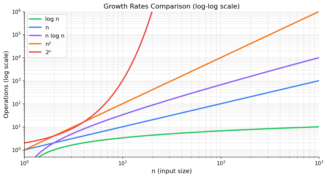
Common Growth Rates
The growth rates appearing most often in algorithm analysis, in increasing order, are:
\[ \Theta(1) \;\prec\; \Theta(\log n) \;\prec\; \Theta(n) \;\prec\; \Theta(n \log n) \;\prec\; \Theta(n^2) \;\prec\; \Theta(n^3) \;\prec\; \Theta(2^n), \]where \(\prec\) means “strictly slower growth.” These correspond to constant, logarithmic, linear, linearithmic, quadratic, cubic, and exponential complexity. The practical significance becomes clear when the problem size doubles from \(n\) to \(2n\): a constant-time algorithm is unaffected; a logarithmic one gains only one extra unit of time; a linear one doubles; a quadratic one quadruples; an exponential one squares.
Any polynomial \(f(n) = c_d n^d + \cdots + c_0\) with \(c_d > 0\) satisfies \(f(n) \in \Theta(n^d)\), since the limit \(f(n)/n^d \to c_d\). Also, \(\log(n!) = \Theta(n \log n)\), a fact used in lower bound arguments.
Analyzing Algorithms in Practice
To analyze a concrete algorithm, we identify the elementary operations (each costing \(\Theta(1)\)), sum their counts as the algorithm executes, and simplify using the rules above.
For a simple nested loop, we work from the inside out. Consider:
Test1(n):
  sum <- 0
  for i <- 1 to n do
    for j <- i to n do
      sum <- sum + (i - j)^2
  return sum
The innermost statement executes \(\Theta(1)\) work. The inner loop runs \(n - i + 1\) times for each \(i\). Summing over \(i\):
\[ \sum_{i=1}^{n} (n - i + 1) = \sum_{k=1}^{n} k = \frac{n(n+1)}{2} \in \Theta(n^2). \]So Test1 runs in \(\Theta(n^2)\) time.
When an algorithm has branches or data-dependent early exits, proving a tight bound may require establishing \(O\) and \(\Omega\) separately. For \(O\), use upper bounds on loop counts; for \(\Omega\), exhibit a specific family of inputs that always hit the worst case.
Useful Summation Formulas
Several standard series appear frequently:
Arithmetic series: \(\displaystyle\sum_{i=0}^{n-1}(a + di) = na + \frac{dn(n-1)}{2} \in \Theta(n^2)\) when \(d \neq 0\).
Geometric series: \(\displaystyle\sum_{i=0}^{n-1} r^i = \frac{r^n - 1}{r - 1} \in \Theta(r^{n-1})\) for \(r > 1\), and \(\in \Theta(1)\) for \(0 < r < 1\).
Harmonic series: \(\displaystyle H_n = \sum_{i=1}^{n} \frac{1}{i} = \ln n + \gamma + o(1) \in \Theta(\log n)\), where \(\gamma \approx 0.5772\) is the Euler–Mascheroni constant.
Power sums: \(\displaystyle\sum_{i=1}^{n} i^k \in \Theta(n^{k+1})\) for \(k \geq 0\).
Case Study: Analysis of MergeSort
Merge sort recursion tree for 8 elements — divide-and-conquer, O(n log n) total work.
MergeSort is the canonical example of divide-and-conquer analysis. The algorithm splits the input array in half, recursively sorts each half, and then merges the two sorted halves. In pseudocode:
MergeSort(A, l, r):
  if r <= l: return
  m <- floor((l + r) / 2)
  MergeSort(A, l, m)
  MergeSort(A, m+1, r)
  Merge(A, l, m, r)
The Merge procedure takes two adjacent sorted subarrays A[l..m] and A[m+1..r] and merges them using an auxiliary array S. It scans both halves with two pointers, always copying the smaller front element into the output. This takes exactly \(r - l + 1\) steps, so merging \(n\) elements costs \(\Theta(n)\).
Let \(T(n)\) be the worst-case running time of MergeSort on an array of length \(n\). The two recursive calls handle halves of size \(\lceil n/2 \rceil\) and \(\lfloor n/2 \rfloor\), and the merge costs \(\Theta(n)\), giving the recurrence:
\[ T(n) = T\!\left(\left\lceil \tfrac{n}{2} \right\rceil\right) + T\!\left(\left\lfloor \tfrac{n}{2} \right\rfloor\right) + \Theta(n), \qquad T(1) = \Theta(1). \]When \(n = 2^k\) is a power of two, the floors and ceilings vanish, yielding the clean recurrence \(T(n) = 2T(n/2) + cn\). Unrolling this \(k = \log_2 n\) levels produces a recursion tree: at level \(j\), there are \(2^j\) subproblems of size \(n/2^j\), each doing \(cn/2^j\) work merging, for a total of \(cn\) work per level. With \(\log n\) levels, the total is \(cn \log n\), giving:
This analysis generalizes to all \(n\) by a careful argument on the exact recurrence with floors and ceilings. The following recurrence table summarizes several important divide-and-conquer patterns:
| Recurrence | Solution | Example |
|---|---|---|
| \(T(n) = T(n/2) + \Theta(1)\) | \(\Theta(\log n)\) | Binary search |
| \(T(n) = 2T(n/2) + \Theta(n)\) | \(\Theta(n \log n)\) | MergeSort |
| \(T(n) = 2T(n/2) + \Theta(\log n)\) | \(\Theta(n)\) | Heapify |
| \(T(n) = T(cn) + \Theta(n)\) for \(0 < c < 1\) | \(\Theta(n)\) | QuickSelect (avg) |
| \(T(n) = T(\sqrt{n}) + \Theta(1)\) | \(\Theta(\log \log n)\) | Interpolation search |
Once a solution is conjectured, it can usually be verified by substitution (induction). More systematic techniques appear in CS 341.
Chapter 2: Priority Queues and Heaps
Abstract Data Types and the Priority Queue
A recurring theme in this course is the separation between what a data structure does (its abstract interface) and how it does it (its concrete implementation). An abstract data type (ADT) specifies a collection of data and a set of operations on that data, with no commitment to any particular internal representation. Different realizations of the same ADT can offer radically different performance characteristics.
The Stack ADT (push/pop, LIFO order) and the Queue ADT (enqueue/dequeue, FIFO order) are familiar examples, both realizable with arrays or linked lists. In this chapter we study a richer ADT: the priority queue.
insert(x): add item \(x\) with its associated key to the collection.
deleteMax(): remove and return the item with the largest key.
A minimum-oriented priority queue replaces deleteMax with deleteMin; the two are symmetric and can be interconverted by negating keys. Applications abound: a task scheduler processes jobs in order of urgency; a simulation system fires events in chronological order; an event-driven game engine processes collisions by time. And, as we will see, priority queues can sort.
PQ-Sort and the Challenge of Implementation
Any priority queue can be turned into a sorting algorithm. Given an array \(A[0..n-1]\), insert all \(n\) elements, then extract them in order via deleteMax:
PQ-Sort(A):
  initialize PQ to an empty priority queue
  for k <- 0 to n-1 do
    PQ.insert(A[k])
  for k <- n-1 down to 0 do
    A[k] <- PQ.deleteMax()
The total time is \(O(n + n \cdot \text{insert} + n \cdot \text{deleteMax})\). The choice of implementation determines the practical cost:
If we use an unsorted array, insertion is \(O(1)\) (append to the end, expanding with doubling if needed — amortized \(O(1)\) per insert), but deleteMax must scan the whole array, costing \(O(n)\). PQ-Sort with an unsorted array is \(\Theta(n^2)\), which corresponds exactly to selection sort.
If we use a sorted array, deleteMax is \(O(1)\) (remove from the end), but maintaining sorted order requires inserting each new element into its correct position in \(O(n)\) time. PQ-Sort with a sorted array gives insertion sort, also \(\Theta(n^2)\).
Both naive approaches are quadratic. To do better, we need a data structure that balances the cost of insertion and deletion, achieving \(O(\log n)\) for each. The answer is the binary heap.
Binary Heaps: Structure and Representation
Structural property: All levels are completely filled except possibly the last, which is filled left-to-right (i.e., the tree is a complete binary tree).
Heap-order property: For every node \(i\), the key of \(i\)'s parent is greater than or equal to the key of \(i\).
The structural property ensures the tree is “as balanced as possible.” An immediate consequence is:
Proof sketch. A complete binary tree with all levels full has height \(\lfloor \log_2 n \rfloor\). The last (possibly incomplete) level can add at most a constant factor. Since any binary tree with \(n\) nodes has height at least \(\log_2(n+1) - 1 \in \Omega(\log n)\), and the structural property gives height at most \(\lfloor \log_2 n \rfloor \in O(\log n)\), the height is \(\Theta(\log n)\).
The heap-order property ensures the maximum is always at the root, giving \(O(1)\) access to the maximum element.
Binary max-heap — complete binary tree with heap-order property, and its array representation.
Array Representation
Heaps are stored compactly in an array, not as a linked tree. Level-order traversal gives the mapping: the root goes to A[0], then the two children of the root go to A[1] and A[2], and so on. For a heap of size \(n\) stored in A[0..n-1]:
Index of root:           0
Left child of A[i]:      A[2i + 1]
Right child of A[i]:     A[2i + 2]
Parent of A[i] (i != 0): A[floor((i-1)/2)]
Last node:               A[n - 1]
This is illustrated by the following example heap with keys [50, 29, 34, 27, 15, 8, 10, 23, 26]:
             50            <- A[0]
           /    \
         29      34        <- A[1], A[2]
        /  \    /  \
       27  15  8   10      <- A[3..6]
      / \
     23  26                <- A[7], A[8]
The array representation eliminates the memory overhead of pointers entirely, and all navigation formulas are simple arithmetic. In practice, implementation should hide these formulas behind helper functions root(), parent(i), leftChild(i), etc., to improve readability and correctness.
Heap Operations
Insertion: Fix-Up (Bubble Up)
To insert a new key \(x\) into a heap of size \(n\), place \(x\) at position A[n] (the next available leaf position) and then restore the heap-order property by bubbling up:
fix-up(A, k):
  while parent(k) exists and A[parent(k)] < A[k]:
    swap A[k] and A[parent(k)]
    k <- parent(k)
The new element climbs toward the root, swapping with its parent each time its key is larger. It stops when either it reaches the root or its parent’s key is at least as large. Since the heap has height \(\Theta(\log n)\), fix-up traverses at most \(\Theta(\log n)\) edges.
Time: \(O(\log n)\).
DeleteMax: Fix-Down (Bubble Down)
To remove the maximum (the root), we cannot simply delete A[0] without leaving a gap. Instead, swap A[0] with the last leaf A[n-1], reduce the heap size by one (the former root is now outside the heap at A[n-1]), and restore the heap-order property by bubbling down from the root:
fix-down(A, n, k):
  while k is not a leaf:
    j <- left child of k
    if j is not the last node and A[j+1] > A[j]:
      j <- j + 1         // j is now the larger child
    if A[k] >= A[j]: break
    swap A[j] and A[k]
    k <- j
At each step, the displaced element is swapped with the larger of its two children. This guarantees that after the swap, both the swapped element and the child that did not move still satisfy the heap-order property with respect to their own subtrees. The procedure runs in \(O(\log n)\) time.
The full deleteMax operation wraps fix-down:
deleteMax():
  l <- last(size)
  swap A[root()] and A[l]
  decrease size
  fix-down(A, size, root())
  return A[l]
Both insert and deleteMax run in \(O(\log n)\) time, and PQ-Sort with a heap implementation takes \(O(n \log n)\).
Building a Heap: Heapify in Linear Time
When all \(n\) elements are available in advance, there is a much faster way to build a heap than inserting elements one by one.
Approach 1 (Bubble-up): Insert elements sequentially, running fix-up after each insertion. This is \(\Theta(n \log n)\) in the worst case: elements near the end of the array may travel all the way to the root.
Approach 2 (Heapify — Bubble-down): Observe that all leaves are already trivially valid single-element heaps. Work backwards from the last internal node to the root, applying fix-down at each position:
heapify(A):
  n <- A.size()
  for i <- parent(last(n)) downto 0:
    fix-down(A, n, i)
The last internal node is at index parent(n-1) = floor((n-2)/2).
heapify runs in \(\Theta(n)\) time.Proof. The key observation is that nodes near the bottom of the tree have small subtrees, and fix-down at those nodes is cheap. At height \(h\) above the leaves, there are at most \(\lceil n/2^{h+1} \rceil\) nodes, and fix-down costs at most \(O(h)\). Summing over all heights:
\[ \sum_{h=0}^{\lfloor \log n \rfloor} \left\lceil \frac{n}{2^{h+1}} \right\rceil \cdot O(h) = O\!\left(n \sum_{h=0}^{\infty} \frac{h}{2^h}\right) = O(n), \]since the series \(\sum_{h=0}^{\infty} h/2^h = 2\) converges. Therefore heapify is \(O(n)\); and clearly it is \(\Omega(n)\) since it must examine each element, so the bound is \(\Theta(n)\).
This is a striking result: despite each individual fix-down taking \(O(\log n)\) time, the combined cost of all fix-downs is only linear, because most nodes sit near the bottom and their fix-downs terminate quickly.
HeapSort
Heapify combined with repeated deleteMax gives an elegant in-place sorting algorithm. Crucially, we reuse the input array as the heap, avoiding any extra space:
HeapSort(A, n):
  // Phase 1: build the heap in-place
  for i <- parent(last(n)) downto 0:
    fix-down(A, n, i)
  // Phase 2: extract elements in sorted order
  while n > 1:
    swap A[root()] and A[last(n)]
    decrease n
    fix-down(A, n, root())
In Phase 1, heapify establishes the max-heap in \(\Theta(n)\) time. In Phase 2, we repeatedly swap the maximum (at the root) to the end of the current heap, shrink the heap by one, and restore the heap property. After \(n-1\) extractions, the array is sorted in ascending order.
Phase 2 performs \(n-1\) fix-down operations on heaps of decreasing size. Each fix-down costs \(O(\log n)\), so Phase 2 is \(O(n \log n)\). The total running time is \(\Theta(n) + O(n \log n) = O(n \log n)\). Since Phase 2 also requires \(\Omega(n \log n)\) in the worst case (a sorted-order input forces each fix-down to traverse the full height), HeapSort is \(\Theta(n \log n)\).
HeapSort has the remarkable property of using only \(O(1)\) auxiliary space (beyond the input array itself), unlike MergeSort which needs \(\Theta(n)\) extra space. It is the only \(\Theta(n \log n)\) sorting algorithm we have seen with this property.
The Selection Problem
We close this chapter with the selection problem: given an array \(A\) of \(n\) numbers and an index \(0 \leq k < n\), find the element that would appear at position \(k\) in the sorted array. Finding the median is the special case \(k = \lfloor n/2 \rfloor\).
Heaps offer several approaches:
Solution 1 (repeated scan): Make \(k\) passes, deleting the maximum each time. Cost: \(\Theta(kn)\), which is \(\Theta(n^2)\) for the median.
Solution 2 (sort first): Sort, then index. Cost: \(\Theta(n \log n)\).
Solution 3 (sliding min-heap): Scan the array, maintaining a min-heap of the \(k\) largest elements seen so far. The top of the min-heap is the \(k\)th largest. Cost: \(\Theta(n \log k)\).
Solution 4 (heapify then extract): Call heapify to build a max-heap in \(\Theta(n)\), then call deleteMax exactly \(k\) times. Cost: \(\Theta(n + k \log n)\).
For the median (\(k = n/2\)), Solutions 2–4 all give \(\Theta(n \log n)\). The question of whether selection can be done faster — in linear time — is addressed in Chapter 3 via the QuickSelect algorithm.
Advanced Heap Structures
The binary heap is an excellent all-around priority queue: simple to implement, cache-friendly in its array layout, and \(O(\log n)\) for both insert and deleteMax. Its one significant limitation is the merge operation. Given two binary heaps of sizes \(n_1\) and \(n_2\), the only known approach using the array representation is to concatenate the two arrays and run heapify, which costs \(\Theta(n_1 + n_2)\) — linear in the combined size. For applications that frequently merge priority queues (external sorting, network routing, Dijkstra’s algorithm with edge relaxations across components), this linear merge cost is a real bottleneck. Two alternative structures overcome it: meldable heaps achieve \(O(\log n)\) expected merge time through randomisation, and binomial heaps achieve \(O(\log n)\) worst-case merge time through a more elaborate structural invariant.
Meldable Heaps
A meldable heap is a binary tree satisfying the heap-order property — every node’s key is at least as large as the keys of its children — but with no structural property whatsoever. The tree can be completely skewed, arbitrarily unbalanced, or have height anywhere from \(\Theta(\log n)\) to \(\Theta(n)\). Abandoning the structural property is what makes merging tractable.
All priority queue operations reduce to a single subroutine: merge(P1, P2), which combines two meldable heaps into one. The algorithm is recursive and randomised:
Input: roots r1, r2 of two meldable heaps (r1 is not null)
1. If r2 is null, return r1
2. If r1.key < r2.key, swap r1 and r2
3. Randomly pick one of r1's two children, call it c (with equal probability for each child)
4. Replace c with merge(r2, c)
5. Return r1
The key insight is step 2: by ensuring the heap with the larger root plays the role of r1, we guarantee that r1’s root remains the maximum in the merged heap, preserving the heap-order property from the top down. The random choice of which child to recurse into is the trick that keeps the expected cost small.
The other operations are immediate reductions to merge:
- insert(k): Create a new single-node heap \(P'\) containing key \(k\). Call
merge(P, P'). This is \(O(\log n)\) expected. - deleteMax: The maximum is at the root. Remove it, exposing two sub-heaps \(P_L\) and \(P_R\) rooted at the root’s two children. Call
merge(P_L, P_R). This is \(O(\log n)\) expected.
Expected runtime of merge. The merge algorithm traces a random downward walk in each of the two heaps simultaneously: at each level, we pick a child uniformly at random and descend into it. The walk terminates when it hits an empty subtree. The run-time of merge is therefore proportional to the total length of these two walks.
The proof is a clean induction on \(n\). Let \(T(n)\) denote this expected length. The base case \(n=1\) is immediate: the walk visits exactly 1 node and \(\log 2 = 1\). For \(n > 1\), let the left and right subtrees have sizes \(n_L\) and \(n_R\) with \(n_L + n_R = n - 1\). With probability \(1/2\) we go left (expected total length \(1 + T(n_L)\)) and with probability \(1/2\) we go right (expected total length \(1 + T(n_R)\)), so
\[ T(n) \leq 1 + \frac{1}{2}T(n_L) + \frac{1}{2}T(n_R) \leq 1 + \frac{1}{2}\log(n_L+1) + \frac{1}{2}\log(n_R+1). \]By the concavity of \(\log\), and using \(\frac{1}{2}(n_L+1) + \frac{1}{2}(n_R+1) = \frac{n+1}{2}\),
\[ T(n) \leq 1 + \log\!\left(\frac{n+1}{2}\right) = 1 + \log(n+1) - 1 = \log(n+1), \]completing the induction. Since merge does two such walks (one in each heap), its expected run-time is \(O(\log n_1 + \log n_2) = O(\log n)\) where \(n = n_1 + n_2\).
The worst case for merge is still \(\Theta(n)\) — a maximally skewed heap where every random choice descends to the lowest leaf — but this event has probability \(2^{-n}\), so it is essentially irrelevant in practice.
Binomial Heaps
Meldable heaps are conceptually simple but offer only expected guarantees. Binomial heaps replace randomisation with a carefully engineered structural invariant that yields \(O(\log n)\) worst-case merge time.
Binomial trees. The building block is a family of trees \(B_0, B_1, B_2, \ldots\) defined recursively:
- \(B_0\) is a single node.
- \(B_k\) is formed by taking two copies of \(B_{k-1}\) and making one the leftmost child of the other’s root.
(1) \(B_k\) has exactly \(2^k\) nodes.
(2) \(B_k\) has height \(k\).
(3) The root of \(B_k\) has exactly \(k\) children.
(4) The children of \(B_k\)'s root are \(B_0, B_1, \ldots, B_{k-1}\) (from right to left).
The name “binomial” reflects that at depth \(d\), \(B_k\) has exactly \(\binom{k}{d}\) nodes — the binomial coefficient. The properties follow easily from the recursive definition by induction.
Binomial heap structure. A binomial heap is a collection (list) of binomial trees such that no two trees have the same order \(k\). Given a heap of size \(n\), write \(n\) in binary: the collection contains \(B_k\) if and only if the \(k\)-th bit of \(n\) is 1. For example, \(n = 13 = 1101_2\) means the heap contains trees \(B_0\), \(B_2\), and \(B_3\) (13 = 1 + 4 + 8 nodes total). Since the binary representation of \(n\) has at most \(\lfloor \log n \rfloor + 1\) bits, a binomial heap contains at most \(\lfloor \log n \rfloor + 1\) trees.
Each tree satisfies the heap-order property: every node’s key is at least as large as the keys of all nodes in its subtrees. The maximum of the entire heap is therefore the maximum among the roots of the constituent binomial trees, found in \(O(\log n)\) by scanning the root list.
Merging two binomial trees. If we have two copies of \(B_k\), we can merge them into a single \(B_{k+1}\) in \(O(1)\) time: compare the two roots, make the smaller root a child of the larger root (to preserve heap order), and the former left subtrees attach appropriately. This mirrors binary addition: two trees of order \(k\) produce one carry of order \(k+1\).
All operations in \(O(\log n)\). Merging two binomial heaps of sizes \(n_1\) and \(n_2\) is exactly like adding two binary numbers: walk through the tree lists from smallest order to largest, combining any two trees of equal order into a carry for the next order. The process visits at most \(O(\log n)\) trees total and each combining step is \(O(1)\), giving \(O(\log n)\) merge.
Insert is a degenerate merge: a single new element is a \(B_0\), and merging it into the existing heap propagates at most \(O(\log n)\) carries. DeleteMax finds the root list’s maximum in \(O(\log n)\), removes its tree \(B_k\), then splits \(B_k\) into its children \(B_0, B_1, \ldots, B_{k-1}\) — which themselves form a valid binomial heap of size \(2^k - 1\) — and merges that back into the remainder in \(O(\log n)\). All standard priority queue operations thus cost \(O(\log n)\) in the worst case.
Comparison. The binary heap remains preferable when merge is not required: the array layout gives excellent cache behaviour and small constant factors. But if the application merges heaps frequently, binomial heaps (or meldable heaps for a simpler implementation) are the right choice. A further refinement, Fibonacci heaps, achieves amortised \(O(1)\) insert and decreaseKey, which is exploited by Dijkstra’s algorithm in dense graphs — but that analysis is reserved for a later course.
Chapter 3: Sorting
The Selection Problem Revisited: QuickSelect
The heap-based selection algorithms of Chapter 2 achieve \(\Theta(n + k \log n)\) time. For median finding with \(k = n/2\), this is \(\Theta(n \log n)\) — the same cost as sorting. Can we find the \(k\)th element in \(O(n)\) time, for any fixed \(k\)?
The QuickSelect algorithm answers yes, in the average case. It is built from two subroutines that are also central to QuickSort.
The Partition Subroutine
choose-pivot(A) selects an index \(p\); the simplest strategy returns the rightmost index.
partition(A, p) rearranges \(A\) so that all elements smaller than the pivot \(v = A[p]\) appear to its left, and all elements larger appear to its right, returning the final index \(i\) of \(v\):
After partition: A[0..i-1] <= v == A[i] <= A[i+1..n-1]
A conceptually simple implementation creates auxiliary lists small and large and concatenates them. More practically, Hoare’s in-place partition uses two pointers scanning from opposite ends:
partition(A, p):
  swap(A[n-1], A[p])
  i <- -1, j <- n-1, v <- A[n-1]
  loop:
    do i <- i+1 while i < n and A[i] < v
    do j <- j-1 while j > 0 and A[j] > v
    if i >= j: break
    else: swap(A[i], A[j])
  swap(A[n-1], A[i])
  return i
The left pointer i advances until it finds an element \(\geq v\); the right pointer j retreats until it finds an element \(\leq v\). When both are “stuck,” we swap the out-of-place pair and repeat. When the pointers cross, the pivot is swapped into its final position. This runs in \(\Theta(n)\) time and uses \(O(1)\) extra space.
The QuickSelect Algorithm
quick-select(A, k):
  p <- choose-pivot(A)
  i <- partition(A, p)
  if i == k: return A[i]
  else if i > k: return quick-select(A[0..i-1], k)
  else: return quick-select(A[i+1..n-1], k - i - 1)
After partitioning, the pivot is in its correct sorted position \(i\). If \(i = k\), we are done. If \(i > k\), the \(k\)th element is in the left sub-array; if \(i < k\), it is in the right sub-array. Only one recursive call is made (unlike QuickSort, which makes two).
Worst-case analysis: If the pivot always lands at one extreme (e.g., the array is sorted and we always pick the rightmost element), each call reduces the problem by only 1:
\[ T(n) = T(n-1) + cn \implies T(n) \in \Theta(n^2). \]Average-case analysis: Assume all \(n!\) permutations of the input are equally likely (or equivalently, that the relative order of elements is what matters — the sorting permutation model). For each pivot index \(i\) (which occurs for \((n-1)!\) out of \(n!\) permutations), the recursive call has size at most \(\max(i, n-i-1)\). Therefore:
\[ T(n) \leq cn + \frac{1}{n} \sum_{i=0}^{n-1} \max\{T(i),\, T(n-i-1)\}. \]Proof sketch. Assume \(T(n) \leq an\) for some constant \(a\) to be determined. The sum \(\frac{1}{n}\sum_{i=0}^{n-1}\max\{T(i), T(n-i-1)\}\) can be bounded by noting that \(\max(T(i), T(n-i-1)) \leq T(n-1)\) in the worst case, but on average the pivot splits the array roughly in half. A careful calculation (treating the recurrence as a telescoping inequality) shows that \(T(n) \leq 4cn\), confirming the \(O(n)\) bound. The \(\Omega(n)\) lower bound is trivial since we must read all inputs.
Randomized Algorithms
The average-case result above assumed a uniform distribution over input permutations. In practice, adversarial or highly structured inputs can trigger the worst case. Randomized algorithms shift the source of variability from the input (which we cannot control) to the random choices made by the algorithm (which we can analyze in expectation).
For a randomized algorithm, we define the expected running time on instance \(I\) as:
\[ T^{(\text{exp})}(I) = \mathbb{E}[T(I, R)] = \sum_{R} T(I, R) \cdot \Pr[R], \]where \(R\) ranges over all possible random choices. The worst-case expected running time is then \(\max_{\text{Size}(I)=n} T^{(\text{exp})}(I)\).
There are two natural ways to randomize QuickSelect:
Shuffle first: Randomly permute the input before running the deterministic algorithm. After shuffling, every permutation is equally likely regardless of the original input, so the expected running time equals the average-case deterministic running time: \(\Theta(n)\).
Random pivot: Simply select the pivot index uniformly at random:
choose-pivot2(A): return random(n)
With probability \(1/n\) the pivot lands at each index \(i\), so the analysis is identical to the average-case analysis: the expected running time is \(\Theta(n)\).
The random-pivot approach is generally preferred in practice because it is simpler and avoids the overhead of a full shuffle. There exists a deterministic linear-time selection algorithm (the “median of medians” method), but it is slower by a constant factor and is deferred to CS 341.
QuickSort
QuickSort, developed by C.A.R. Hoare in 1960, applies the same partition idea to sorting by recursing on both sides of the pivot:
quick-sort(A):
  if n <= 1: return
  p <- choose-pivot(A)
  i <- partition(A, p)
  quick-sort(A[0..i-1])
  quick-sort(A[i+1..n-1])
Worst case: If the pivot always lands at an extreme position, the recurrence is the same as for QuickSelect: \(T(n) = T(n-1) + \Theta(n)\), giving \(T(n) \in \Theta(n^2)\).
Best case: If the pivot always splits the array exactly in half, we get the MergeSort recurrence \(T(n) = 2T(n/2) + \Theta(n)\), giving \(T(n) \in \Theta(n \log n)\).
Average case: Over all \(n!\) permutations, with probability \(1/n\) the pivot has rank \(i\), leaving sub-arrays of sizes \(i\) and \(n-i-1\). The recurrence is:
\[ T^{(\text{avg})}(n) = cn + \frac{1}{n} \sum_{i=0}^{n-1} \left[T^{(\text{avg})}(i) + T^{(\text{avg})}(n-i-1)\right], \qquad n \geq 2. \]Proof sketch. Multiply both sides by \(n\) and subtract the analogous equation for \(n-1\) to telescoping. One obtains \(nT(n) - (n-1)T(n-1) = cn^2 + 2T(n-1)\), which rearranges to \(T(n)/(n+1) = T(n-1)/n + c'\) for an appropriate constant \(c'\). Unrolling gives \(T(n)/(n+1) = \sum_{k=2}^{n} c' \approx c' \ln n\), so \(T(n) \approx c'(n+1)\ln n \in \Theta(n \log n)\).
Using a random pivot (choose-pivot2) gives an expected running time of \(\Theta(n \log n)\), with the same analysis since the randomness is equivalent to a uniform permutation of the input.
Practical Improvements
Several engineering refinements make QuickSort the fastest sorting algorithm in practice for most inputs:
Auxiliary space: The recursion stack uses \(\Omega(\text{recursion depth})\) space — \(\Theta(n)\) in the worst case. By always recursing on the smaller sub-array first and replacing the larger recursion with a loop (tail-call optimization), the stack depth is reduced to \(\Theta(\log n)\) in the worst case.
Cutoff to insertion sort: When sub-arrays become small (say, \(n \leq 10\)), stop recursing and instead run a final pass of insertion sort over the entire array. Since each element is within 10 positions of its final location at that point, the insertion sort pass costs \(O(n)\) total.
Three-way partition: For inputs with many duplicate keys, the two-way partition can degrade. A three-way partition produces three regions — elements less than, equal to, and greater than the pivot — and recurses only on the outer two. This reduces the work on the duplicate elements to zero.
Lower Bound for Comparison-Based Sorting
The sorting algorithms seen so far — Selection Sort, Insertion Sort, MergeSort, HeapSort, QuickSort — all operate in the comparison model: elements can only be examined by comparing pairs, and moved around. Under this model, a fundamental lower bound holds.
Proof. Model any deterministic comparison-based sorting algorithm as a decision tree: each internal node represents a comparison between two elements, with two branches for the two outcomes; each leaf is a possible sorted permutation of the input. For the algorithm to correctly sort every input, the decision tree must have at least one leaf for each of the \(n!\) possible input permutations. A binary tree with \(\ell\) leaves has height at least \(\log_2 \ell\). Since \(\ell \geq n!\), the worst-case number of comparisons (the height of the tree) satisfies:
\[ \text{comparisons} \geq \log_2(n!) = \sum_{k=1}^{n} \log_2 k \geq \sum_{k=\lceil n/2 \rceil}^{n} \log_2 k \geq \frac{n}{2} \log_2\!\left(\frac{n}{2}\right) = \frac{n}{2}(\log_2 n - 1) \in \Omega(n \log n). \]Therefore no comparison-based algorithm can beat \(\Omega(n \log n)\) in the worst case. \(\square\)
This is a striking information-theoretic argument: just to communicate which of the \(n!\) permutations is the correct sorted order requires at least \(\log_2(n!)\) bits, and each comparison provides at most one bit.
The result does not apply to algorithms that exploit additional structure of the keys — for example, when keys are integers in a bounded range.
Non-Comparison-Based Sorting: Radix and Count Sort
When keys are integers (or can be encoded as such), we can beat \(\Omega(n \log n)\) by reading individual digits of the keys rather than comparing whole keys. These algorithms are not in the comparison model.
Single-Digit Bucket Sort
Assume keys are integers with digits from a radix \(R\) alphabet \(\{0, 1, \ldots, R-1\}\). To sort by a single digit \(d\):
Bucket sort creates \(R\) “buckets” \(B[0], B[1], \ldots, B[R-1]\) (each a linked list), distributes each element into the bucket matching its \(d\)th digit, then concatenates the buckets back into the array.
Bucket-Sort(A, d):
  initialize B[0..R-1] as empty lists
  for i <- 0 to n-1:
    append A[i] to B[digit_d(A[i])]
  i <- 0
  for j <- 0 to R-1:
    move all elements of B[j] into A[i++]
Bucket sort is stable: elements with the same digit value appear in the output in the same relative order as in the input. This stability is crucial for multi-digit sorting. Running time: \(\Theta(n + R)\); auxiliary space: \(\Theta(n)\) for the lists.
Count Sort
Bucket sort wastes space on linked list overhead. A space-optimized variant, count sort (also called key-indexed count sort), avoids lists by pre-computing where each group starts:
key-indexed-count-sort(A, d):
  count[0..R-1] <- 0
  for i <- 0 to n-1:
    count[digit_d(A[i])]++
  idx[0] <- 0
  for i <- 1 to R-1:
    idx[i] <- idx[i-1] + count[i-1]
  aux[0..n-1] <- empty array
  for i <- 0 to n-1:
    aux[idx[digit_d(A[i])]] <- A[i]
    idx[digit_d(A[i])]++
  A <- copy(aux)
The count array tallies how many elements have each digit value. The idx array converts those counts into starting positions via prefix sums. Each element is then placed directly at its correct position in the auxiliary array aux. This too runs in \(\Theta(n + R)\) time.
MSD and LSD Radix Sort
For keys with \(m\) digits each, the single-digit sort extends in two natural ways.
MSD-Radix-Sort (Most Significant Digit first) sorts by the leading digit, then recursively sorts each resulting group by the next digit, and so on. This requires managing up to \(R\) recursive subproblems at each level, leading to \(R^m\) potential leaf groups and significant recursion overhead.
LSD-Radix-Sort (Least Significant Digit first) sorts by the last digit first, then the second-to-last, and so on up to the most significant digit. Because count sort is stable, each pass preserves the ordering established by earlier passes:
LSD-Radix-Sort(A):
  for d <- m down to 1:
    key-indexed-count-sort(A, d)
After sorting by digit \(d\), the loop invariant is that \(A\) is sorted with respect to digits \(d, d+1, \ldots, m\). When digit 1 is processed last, the array is fully sorted.
[123, 230, 021, 320, 210, 232, 101]:After sorting by digit 3 (last):
[230, 320, 210, 021, 101, 232, 123]After sorting by digit 2:
[101, 210, 320, 021, 123, 230, 232]After sorting by digit 1:
[021, 101, 123, 210, 230, 232, 320]Time: Each of the \(m\) passes runs in \(\Theta(n + R)\) time, giving a total of \(\Theta(m(n + R))\). If keys are \(b\)-bit integers and \(R = 2^r\) for some block size \(r\), then \(m = b/r\) and the cost is \(\Theta\!\left(\frac{b}{r}(n + 2^r)\right)\), which is optimized by choosing \(r = \log_2 n\) to give \(\Theta(bn/\log n)\). For fixed-length keys (\(b = O(\log n)\)), this is \(O(n)\) — linear time.
Auxiliary space: \(\Theta(n + R)\).
Sorting: The Big Picture
The following table summarizes the algorithms covered so far:
| Algorithm | Worst-Case | Average-Case | Extra Space |
|---|---|---|---|
| Selection Sort | \(\Theta(n^2)\) | \(\Theta(n^2)\) | \(O(1)\) |
| Insertion Sort | \(\Theta(n^2)\) | \(\Theta(n^2)\) | \(O(1)\) |
| MergeSort | \(\Theta(n \log n)\) | \(\Theta(n \log n)\) | \(\Theta(n)\) |
| HeapSort | \(\Theta(n \log n)\) | \(\Theta(n \log n)\) | \(O(1)\) |
| QuickSort (det.) | \(\Theta(n^2)\) | \(\Theta(n \log n)\) | \(O(\log n)\)* |
| QuickSort (rand.) | \(\Theta(n^2)\)** | \(\Theta(n \log n)\) expected | \(O(\log n)\)* |
| LSD-Radix Sort | \(\Theta(m(n+R))\) | \(\Theta(m(n+R))\) | \(\Theta(n+R)\) |
* With tail-call optimization. ** With probability exponentially small in \(n\).
The \(\Omega(n \log n)\) lower bound applies to all comparison-based algorithms, making MergeSort and HeapSort asymptotically optimal in that model. QuickSort is faster in practice despite its quadratic worst case, because its average-case constant is small. Radix sort sidesteps the lower bound by exploiting the integer structure of keys, achieving linear time when \(m\) and \(R\) are small — but it requires keys that can be decomposed digit-by-digit, unlike fully general comparison-based sorting.
Chapter 4: Dictionaries and Balanced Search Trees
4.1 The Dictionary ADT
A dictionary is one of the most fundamental abstract data types in computer science. Conceptually, it models any collection of items where each item consists of a key and associated data, forming a key-value pair (KVP). Keys are drawn from some totally ordered universe and are assumed to be unique within the dictionary. The three core operations are:
- search(k): locate the item with key \(k\), returning the value or signalling failure.
- insert(k, v): add the pair \((k, v)\) to the collection.
- delete(k): remove the item with key \(k\).
Optional extensions include closestKeyBefore(k), join, isEmpty, size, and various ordered queries. The dictionary appears throughout software engineering under many guises: symbol tables in compilers, DNS lookup tables, in-memory caches, and license plate databases are all dictionaries at heart.
Elementary Implementations
Before diving into sophisticated structures, it pays to know the landscape of naive implementations. We assume throughout that the dictionary holds \(n\) KVPs, each occupying constant space, and that key comparisons take constant time.
An unordered array or linked list stores items in no particular order. Insertion is cheap — simply append or prepend, costing \(\Theta(1)\) — but search and delete both require scanning the entire collection in the worst case, giving \(\Theta(n)\) for each.
An ordered array keeps items sorted by key, enabling binary search and thus \(\Theta(\log n)\) search time. The price is paid on mutation: inserting or deleting a key requires shifting elements to maintain order, costing \(\Theta(n)\) per operation.
Neither naive approach delivers logarithmic time for all three operations simultaneously. The solution lies in tree-based structures.
4.2 Binary Search Trees: A Review
A binary search tree (BST) organises \(n\) KVPs in a rooted binary tree satisfying the BST ordering property: for every node storing key \(k\), every key in the left subtree is strictly less than \(k\), and every key in the right subtree is strictly greater.
          15
         /  \
        6    25
         \   / \
         10 23  29
         /    \   \
        8     24  50
Binary Search Tree — BST ordering property: left subtree < node < right subtree.
Search proceeds by comparison at each node: if the target equals the current key, return it; if the target is smaller, recurse into the left subtree; otherwise recurse right. The process terminates either at the target or at an empty subtree indicating absence. Insert is identical in traversal logic — the new leaf is placed exactly where a search for the new key would have bottomed out.
Deletion handles three cases:
- The target node is a leaf: simply remove it.
- The target node has exactly one non-empty subtree: splice the node out by linking its parent directly to its child.
- The target node has two non-empty subtrees: find the inorder successor (or predecessor) — the smallest key in the right subtree — swap keys, then delete the successor from the right subtree. The successor is guaranteed to have at most one child, reducing this case to case 1 or 2.
All three operations cost \(\Theta(h)\), where \(h\) is the height of the tree, defined as the maximum path length from root to leaf.
The Height Problem
The height of a BST depends critically on insertion order. In the worst case — inserting keys in sorted or reverse-sorted order — the tree degenerates into a path of length \(n - 1 = \Theta(n)\), making every operation linear. In the best case, a perfectly balanced binary tree on \(n\) nodes has height \(\lfloor \log_2(n+1) \rfloor - 1 = \Theta(\log n)\). It can be shown that for a uniformly random insertion sequence, the expected height is also \(\Theta(\log n)\), but an adversary can always force worst-case behaviour. This motivates the need for a self-balancing tree.
4.3 AVL Trees
The AVL tree, introduced by Adel’son-Vel’skiĭ and Landis in 1962, is the classical answer to the BST height problem. It augments the BST with a height-balance property enforced at every node:
The quantity \(\text{height}(R) - \text{height}(L) \in \{-1, 0, +1\}\) is called the balance factor of the node. A balance factor of \(-1\) means the node is left-heavy, \(0\) means balanced, and \(+1\) means right-heavy. Each node stores either its subtree height or its balance factor; the implementation in CS 240 stores heights directly.
Why AVL Trees Have Logarithmic Height
The proof proceeds by counting nodes in the skinniest possible AVL tree. Let \(N(h)\) denote the minimum number of nodes in any height-\(h\) AVL tree. Base cases: \(N(-1) = 0\) (empty tree), \(N(0) = 1\) (single root). For \(h \geq 1\), the thinnest AVL tree of height \(h\) has root, one subtree of height \(h-1\) (the taller one), and one subtree of height \(h-2\) (the shortest the AVL property permits):
\[N(h) = 1 + N(h-1) + N(h-2)\]This is structurally identical to the Fibonacci recurrence shifted by one. Setting \(F_k\) for the \(k\)-th Fibonacci number, one can show \(N(h) = F_{h+3} - 1\). Since Fibonacci numbers grow as \(F_k \approx \phi^k / \sqrt{5}\) where \(\phi = (1+\sqrt{5})/2 \approx 1.618\), we get \(n \geq N(h) \approx \phi^{h+3}/\sqrt{5}\), so \(h \leq \log_\phi(n\sqrt{5}) - 3 = O(\log n)\). The lower bound \(h = \Omega(\log n)\) follows from the fact that any binary tree with \(n\) nodes has height at least \(\lfloor \log_2(n+1) \rfloor - 1\). Together: \(h = \Theta(\log n)\), and all AVL operations cost \(\Theta(\log n)\).
4.4 AVL Insertion and Rotations
AVL rotations — left rotation (right-heavy) and right rotation (left-heavy) restore balance.
To insert \((k, v)\) into an AVL tree:
- Perform the standard BST insertion, obtaining a new leaf \(z\) with height 0.
- Walk back up toward the root, updating heights at each ancestor using
setHeightFromSubtrees. - At the first ancestor \(z\) where the balance factor becomes \(\pm 2\), the AVL property is violated. Perform a restructuring at \(z\) and stop — one restructuring is always sufficient for insertion.
AVL-insert(r, k, v)1. z ← BST-insert(r, k, v)
2. z.height ← 0
3. while z is not the root:
4. z ← parent of z
5. if |z.left.height − z.right.height| > 1 then
6. y ← taller child of z (break ties arbitrarily)
7. x ← taller child of y (prefer left-left or right-right)
8. z ← restructure(x)
9. break // one restructure suffices for insertion
10. setHeightFromSubtrees(z)
The Four Rotation Cases
The key insight is that for any three nodes \(x, y, z\) (grandchild, child, grandparent) and their four subtrees \(A, B, C, D\) in sorted order, there is exactly one perfectly balanced arrangement where the median key becomes the root. The four cases correspond to the four possible shapes of the \(x, y, z\) path.
Right Rotation (left-left case, \(z\) is right-heavy-left or “LL”): \(y\) is the left child of \(z\) and \(x\) is the left child of \(y\).
      z                y
     / \              / \
    y   D    -->     x   z
   / \              / \ / \
  x   C            A  B C  D
 / \
A   B
The operation: set \(y \leftarrow z.\text{left}\), then \(z.\text{left} \leftarrow y.\text{right}\), then \(y.\text{right} \leftarrow z\). Update heights of \(z\) then \(y\). Return \(y\) as the new root of the subtree. Only two pointer changes and two height updates are needed.
Left Rotation (right-right case, RR): the symmetric mirror of the right rotation. \(y\) is the right child of \(z\), \(x\) is the right child of \(y\). The left rotation brings \(y\) up and pushes \(z\) down-left.
Double Right Rotation (left-right case, LR): \(y\) is the left child of \(z\), but \(x\) is the right child of \(y\). A single right rotation would not fix the imbalance. Instead, first apply a left rotation at \(y\) (which transforms this into an LL configuration at \(z\)), then a right rotation at \(z\).
    z                z               x
   / \              / \             / \
  y   D    -->     x   D   -->    y   z
 / \              / \            / \ / \
A   x            y   C          A  B C  D
   / \          / \
  B   C        A   B
Double Left Rotation (right-left case, RL): the symmetric mirror. First a right rotation at \(y\), then a left rotation at \(z\).
The restructure(x) function examines the relative positions of \(x\), \(y = \text{parent}(x)\), and \(z = \text{parent}(y)\) to dispatch to the appropriate case. A memorable rule: the median key among \(x, y, z\) always becomes the new subtree root.
4.5 AVL Deletion
Deletion is more involved. The procedure:
- Perform BST deletion on key \(k\). Let \(z\) be the node that was structurally removed (in the two-children case, this is the inorder successor that got spliced out, not the node originally holding \(k\)).
- Starting from \(z\), walk up toward the root, updating heights and restructuring whenever the balance factor reaches \(\pm 2\).
- Unlike insertion, deletion may require up to \(\Theta(h)\) restructurings — each rotation may fix one imbalance only to expose a new one higher up.
AVL-delete(r, k)1. z ← BST-delete(r, k) // z is child of removed node
2. setHeightFromSubtrees(z)
3. while z is not the root:
4. z ← parent of z
5. if |z.left.height − z.right.height| > 1 then
6. y ← taller child of z
7. x ← taller child of y
8. z ← restructure(x)
9. setHeightFromSubtrees(z) // always continue up
Note the contrast with insertion: there is no break after restructuring. Deletion may propagate violations all the way to the root.
Runtime Summary
| Operation | Cost |
|---|---|
| AVL-search | \(\Theta(\log n)\) worst-case |
| AVL-insert | \(\Theta(\log n)\) worst-case (one restructure) |
| AVL-delete | \(\Theta(\log n)\) worst-case (up to \(O(\log n)\) restructures) |
All operations are dominated by the tree height, which is provably \(\Theta(\log n)\). The AVL tree is thus the first data structure in this course achieving worst-case logarithmic time for all dictionary operations simultaneously.
Amortized Analysis and Scapegoat Trees
The Idea Behind Amortized Analysis
Most complexity analyses focus on the worst-case cost of a single operation. But many data structures exhibit bursty behaviour: most operations are cheap, and occasional operations are expensive. If we charge the full worst-case cost to every operation, we are being pessimistic — the expensive operations cannot happen in every step because the very conditions that make them expensive take many cheap steps to create.
Amortized analysis accounts for this by analysing the total cost of a sequence of \(k\) operations and deriving a bound on the average cost per operation, called the amortized cost. Crucially, this average is taken over any possible sequence of operations in a worst-case sense — it is not an average over random inputs. If the amortized cost of each operation is \(f(n)\), then any sequence of \(k\) operations costs at most \(k \cdot f(n)\) in total.
This definition says that the amortized costs form an “account” that is never overdrawn: the sum of credited amounts always covers the sum of actual costs. An individual amortized cost can be larger than the actual cost for a given step (we are “saving up”), or it can even be zero (we are drawing from savings), as long as the total account balance remains non-negative.
The Potential Function Method
While simple arguments (counting cheap and expensive operations) suffice for textbook examples, a systematic approach is needed for more complex structures. The potential function method provides this.
Given a potential function, define the amortized cost of operation \(O\) as:
\[ T^{\text{amort}}(O) := T^{\text{actual}}(O) + \Phi_{\text{after}} - \Phi_{\text{before}} = T^{\text{actual}}(O) + \Delta\Phi. \]The change in potential \(\Delta\Phi\) acts like a “credit adjustment.” When an operation builds up structural disorder (increasing potential), it pays more than its actual cost. When an expensive operation reduces disorder (decreasing potential), the negative \(\Delta\Phi\) absorbs some of the actual cost. Since \(\Phi\) starts at zero and is always non-negative, the telescoping sum
\[ \sum_{i=1}^k T^{\text{amort}}(O_i) = \sum_{i=1}^k T^{\text{actual}}(O_i) + \Phi(k) - \Phi(0) \geq \sum_{i=1}^k T^{\text{actual}}(O_i) \]confirms that the amortized costs upper-bound the actual costs. The art is in choosing \(\Phi\) so that the amortized costs are small.
Example — dynamic array doubling. When a dynamic array of current size \(n\) fills its capacity, it allocates a new array of double the capacity and copies all elements. The actual copy costs \(\Theta(n)\), but it is preceded by \(n/2\) cheap \(O(1)\) insertions. Define
\[ \Phi = \max\{0,\; 2 \cdot \text{size} - \text{capacity}\}. \]When the array is at half capacity, \(\Phi = 0\). Each cheap insertion increases size by 1 without changing capacity, so \(\Delta\Phi = 2\), giving amortized cost \(1 + 2 = 3 = O(1)\). When the array doubles, size equals capacity so \(\Phi_{\text{before}} = \text{size}\). After doubling, capacity = 2·size so \(\Phi_{\text{after}} = 0\), giving \(\Delta\Phi = -\text{size}\) and amortized cost \(\text{size} + (-\text{size}) = 0\). The expensive copy is fully covered by the accumulated potential, confirming that push is amortized \(O(1)\).
Scapegoat Trees
AVL trees maintain height balance by storing balance information at every node and performing rotations on every insert and delete. Scapegoat trees take a radically different approach: they do not store any balance information, they never perform rotations, but they occasionally rebuild a subtree from scratch into a perfectly balanced BST. The rebuilding is triggered only when a node becomes sufficiently unbalanced, and the amortized analysis shows that the occasional rebuild cost is spread over enough cheap operations to keep the amortized cost logarithmic.
Weight-balance. Fix a parameter \(\alpha \in (1/2, 1)\) (a typical choice is \(\alpha = 2/3\)). For a node \(v\), let \(\text{size}(v)\) denote the number of nodes in the subtree rooted at \(v\).
A BST is an \(\alpha\)-weight-balanced scapegoat tree if every node is \(\alpha\)-weight-balanced. An unbalanced node is called a scapegoat.
Height bound. If every node is \(\alpha\)-weight-balanced, the height is at most \(\log_{1/\alpha} n\). This is because on any root-to-leaf path, each step down into a subtree reduces the size by a factor of at most \(\alpha\), so after \(h\) steps the subtree has size at most \(\alpha^h n \geq 1\), giving \(h \leq \log_{1/\alpha} n = O(\log n)\).
Insert. Perform a standard BST insert, walking down and placing the new key at a leaf. After the insert, walk back up toward the root. If any ancestor \(v\) is now \(\alpha\)-weight-unbalanced — that is, one child has more than \(\alpha \cdot \text{size}(v)\) descendants — then \(v\) is the scapegoat. Rebuild the subtree rooted at \(v\) into a perfectly balanced BST using an \(O(\text{size}(v))\) algorithm (e.g., sort the keys and build recursively from the median). After rebuild, every node in the subtree is \(\alpha\)-balanced.
Delete. Rather than immediately rebuilding, scapegoat trees use lazy deletion: mark the node as deleted without removing it from the tree structure. Deleted nodes participate in size counting (affecting balance checks). When the number of deleted nodes exceeds half the total number of nodes, rebuild the entire tree from scratch (discarding all marked nodes) in \(O(n)\) time.
Amortized analysis. To analyse scapegoat trees with the potential method, define
\[ \Phi(i) := c \cdot \sum_{v \in S} \max\!\bigl\{0,\; |\text{size}(\text{left}(v)) - \text{size}(\text{right}(v))| - 1\bigr\}, \]where the sum is over all nodes \(v\) in the current tree, and \(c > 0\) is a constant to be chosen. The term for each node is the excess imbalance above 1; a perfectly balanced node contributes 0. Clearly \(\Phi(0) = 0\) and \(\Phi(i) \geq 0\) for all \(i\).
For insert (excluding any rebuild): the new node \(z\) has at most \(O(\log n)\) ancestors, and each ancestor’s imbalance term can increase by at most 1, so \(\Delta\Phi \leq c \cdot O(\log n)\). The actual cost of the walk is \(O(\log n)\). Thus \(T^{\text{amort}}(\text{insert}) = O(\log n) + c \cdot O(\log n) = O(\log n)\).
For rebuild at node \(p\) with subtree size \(n_p\): the actual cost is \(O(n_p)\) time units. Before the rebuild, \(p\) was \(\alpha\)-unbalanced, so one of its children had size greater than \(\alpha \cdot n_p\). A short calculation shows \(|\text{size}(\text{left}(p)) - \text{size}(\text{right}(p))| \geq (2\alpha - 1)n_p + 1\), which means the potential contribution of \(p\) alone is at least \(c(2\alpha - 1)n_p\). After a perfect rebuild, every node’s imbalance is at most 1, so all potential contributions within the subtree drop to 0. Therefore \(\Delta\Phi \leq -c(2\alpha-1)n_p\). Setting \(c = 1/(2\alpha - 1)\) (which is positive since \(\alpha > 1/2\)) yields
\[ T^{\text{amort}}(\text{rebuild}) = n_p - c(2\alpha-1)n_p = n_p - n_p = O(1). \]The costly rebuild is entirely paid for by the potential that accumulated during prior insertions into the unbalanced subtree. Combining both cases, every scapegoat tree operation has amortized cost \(O(\log n)\), while worst-case individual operations can cost \(\Theta(n)\) when a large subtree is rebuilt.
Scapegoat trees occupy an interesting niche in the BST design space. They have simpler code than AVL trees (no rotations, no balance fields) while guaranteeing the same \(O(\log n)\) amortized performance. The trade-off is that while AVL trees are \(O(\log n)\) worst-case, scapegoat trees are only \(O(\log n)\) amortized — occasional operations can be slow.
Chapter 5: Skip Lists and Randomized Structures
Treaps: Randomized BSTs
The Core Idea
Both AVL trees and scapegoat trees require the implementation to actively monitor and maintain balance. A fundamentally different approach to randomization asks: what if we assign each key a random priority at insertion time, and then organise the tree to respect both the BST order on keys and a heap order on priorities? The resulting structure is called a treap — a portmanteau of tree and heap.
BST property: for every node \(v\), all keys in \(v\)'s left subtree are less than \(v.k\), and all keys in \(v\)'s right subtree are greater than \(v.k\).
Heap property: for every node \(v\), \(v.p\) is greater than or equal to the priorities of all nodes in \(v\)'s subtree (max-heap on priorities).
A key structural fact: if all \(n\) keys are distinct and all \(n\) priorities are distinct, then the treap structure is uniquely determined by the set of (key, priority) pairs. This is because the node with the highest priority must be the root (heap property), keys smaller than the root’s key must go left and larger ones right (BST property), and the same argument applies recursively within each subtree.
The following small example illustrates the structure. Keys are shown above, priorities below each key:
         key: 10
         pri: 9
        /        \
   key:5         key:14
   pri:7         pri:6
   /   \         /    \
key:3  key:8  key:12  key:17
pri:4  pri:2  pri:5   pri:1
Reading horizontally: 3 < 5 < 8 < 10 < 12 < 14 < 17 (BST order). Reading vertically from root: 9 > 7 > 4, and 9 > 6 > 5 > 1, etc. (heap order). Both invariants hold simultaneously.
Expected Height: O(log n)
The key property of treaps is that when priorities are assigned uniformly at random, the expected height is \(O(\log n)\). The proof rests on a beautiful symmetry argument.
This is because the node with the highest priority must be inserted first (it becomes the root by the heap property), the node with the second highest priority is inserted second, and so on. Since the priority permutation is uniformly random, this insertion order is uniformly random, and by the classical result on randomly built BSTs, the expected height is \(O(\log n)\).
We can make the depth bound more precise using a direct probabilistic argument. Consider nodes \(x_i\) and \(x_j\) with \(i < j\) (so \(x_i < x_j\) in key order). Node \(x_i\) is an ancestor of \(x_j\) in the treap if and only if \(x_i\) has a higher priority than every other node in \(\{x_i, x_{i+1}, \ldots, x_j\}\). By symmetry among the \(j - i + 1\) nodes in this range, the probability that \(x_i\) has the maximum priority is exactly \(1/(j-i+1)\). Therefore
\[ \Pr[x_i \text{ is an ancestor of } x_j] = \frac{1}{j - i + 1}. \]The expected depth of node \(x_j\) equals the expected number of its proper ancestors, which is
\[ \mathbb{E}[\text{depth}(x_j)] = \sum_{i=1}^{j-1} \frac{1}{j-i+1} + \sum_{i=j+1}^{n} \frac{1}{i-j+1} \leq \sum_{m=1}^{n} \frac{1}{m} = H_n, \]where \(H_n = 1 + \frac{1}{2} + \cdots + \frac{1}{n} \approx \ln n\) is the \(n\)-th harmonic number. So the expected depth of any node is at most \(H_n = O(\log n)\), and the expected height of the entire treap is \(O(\log n)\) as well.
This is a stronger statement than the meldable heap analysis: not only is the average depth logarithmic, but the constant factor is exactly the harmonic number, giving a precise expected depth of roughly \(2 \ln n \approx 1.386 \log_2 n\) — slightly worse than the perfectly balanced tree’s \(\log_2 n\), but still \(O(\log n)\).
Operations
Search. A treap is a BST, so search proceeds by the standard BST algorithm: compare the query key against the root, then recurse into the left or right subtree. Since the expected height is \(O(\log n)\), search takes \(O(\log n)\) expected time.
Insert. To insert a new key \(k\):
- Assign \(k\) a priority chosen uniformly at random from \(\{0, \ldots, n\}\) (where \(n\) is the new size).
- Walk down the BST to the leaf position where \(k\) belongs, and insert \(k\) there as a new leaf.
- The new leaf may violate the heap property (its priority may be larger than its parent’s). Fix this by performing rotations: if the new node has a higher priority than its parent, rotate the parent down (a single rotation). Repeat until the heap property is restored or the node reaches the root.
The rotation used is the same as in AVL trees but driven by a different criterion. A right rotation at node \(y\) makes \(y\)’s left child \(x\) the new local root and attaches \(y\) as \(x\)’s right child, while \(x\)’s former right subtree becomes \(y\)’s new left subtree. Left rotations are symmetric. A single rotation adjusts the parent-child relationship between two nodes while preserving both the BST order and the heap order (because a rotation only changes one edge).
The expected number of rotations during insert is at most 2, since each rotation moves the new node one level up and the node ascends at most depth levels.
Delete. Deletion is conceptually the reverse of insertion:
- Find the node with key \(k\) using standard BST search.
- Set its priority to \(-\infty\) (conceptually).
- Since the node now has the lowest priority in its neighbourhood, the heap property forces it to rotate downward. Perform rotations — always rotating the higher-priority child up — until the target node becomes a leaf.
- Remove the leaf.
At each step, the node being deleted trades places with its higher-priority child, maintaining both the BST and heap invariants throughout. The expected number of rotations is \(O(\log n)\) (proportional to the depth of the deleted node).
All operations in \(O(\log n)\) expected time. Because the treap’s shape is determined solely by the random priorities, no fixed input sequence of insertions and deletions can force the treap into a bad shape. An adversary who knows the algorithm but not the random choices cannot construct a worst-case sequence. This is the essential advantage over deterministic BSTs: the randomisation makes the algorithm’s behaviour independent of the input distribution.
Treaps in Practice
Treaps require storing one extra integer (the priority) per node, plus a pointer to the parent for rotation purposes, giving a small constant-factor space overhead compared to a plain BST. This is smaller than the overhead of AVL trees (which also need parent pointers and a balance field) and roughly comparable to red-black trees.
In practice, treaps are valued for their simplicity: the insert and delete algorithms are shorter and less error-prone than AVL or red-black tree implementations, because the rotation logic is driven entirely by two simple invariants rather than case analyses on colour or height. Split and join operations on treaps (splitting a treap at a given key, or joining two treaps whose keys are disjoint) can also be implemented in \(O(\log n)\) expected time, which makes treaps useful as a building block for more complex data structures such as order-statistic trees and interval trees.
The relationship between treaps and skip lists — both randomised dictionary implementations introduced in this chapter — is worth noting. Both achieve \(O(\log n)\) expected time for all operations by injecting randomness into the structure rather than the input order. Skip lists use coin flips to determine the height of each tower; treaps use random priorities to determine the shape of a BST. In both cases, the adversary cannot predict the outcome of our random choices, so no input sequence is inherently pathological.
5.1 The Motivation for Randomization
By the end of Module 4, we have a clear picture of the dictionary landscape. Unordered structures offer cheap insertion but expensive search. The ordered array achieves fast search at the cost of slow mutation. AVL trees deliver \(\Theta(\log n)\) across the board, but their implementation is non-trivial — rotations require careful bookkeeping and the code for deletion in particular is intricate.
A natural question is: can we achieve the same asymptotic performance with a simpler structure? The average-case height of a randomly built BST (over all insertion permutations) is \(\Theta(\log n)\), which hints that “most” BSTs are well-shaped. The challenge is that an adversary can always choose an insertion order that defeats us. Randomization is the remedy: if we make random choices ourselves during insertion, no fixed input sequence can force bad behaviour. The expected performance is then over our own coin flips, not over the input distribution.
The skip list, introduced by William Pugh in 1990, is the canonical randomized dictionary. It achieves \(O(\log n)\) expected time for all operations with a structure that is both elegant and easy to implement.
5.2 Skip List Structure
A skip list \(S\) is a hierarchy of sorted linked lists \(S_0, S_1, \ldots, S_h\), where:
- \(S_0\) is the base list, containing all \(n\) KVPs in non-decreasing order of key, plus two sentinel nodes with keys \(-\infty\) and \(+\infty\) at the two ends.
- Each \(S_i\) for \(i > 0\) is a subsequence of \(S_{i-1}\), meaning \(S_0 \supseteq S_1 \supseteq \cdots \supseteq S_h\).
- The topmost list \(S_h\) contains only the two sentinels.
Each key present in multiple lists forms a tower of nodes, one per level, linked vertically. Every node \(p\) in the structure supports two pointer operations: after(p) returns the next node in the same list, and below(p) returns the corresponding node one level down.
S3:  -inf ------------------------------------ +inf
S2:  -inf ---------- 37 --------- 65 -- 94 -- +inf
S1:  -inf -- 23 --- 37 --------- 65 -- 94 -- +inf
S0:  -inf -- 23 -- 37 -- 44 -- 65 -- 69 -- 79 -- 83 -- 87 -- 94 -- +inf
The skip list is accessed via a pointer to the topmost-left node (the \(-\infty\) sentinel in \(S_h\)).
5.3 Search
The search algorithm exploits the layered structure to skip large blocks of the base list. Starting at the topmost sentinel, the algorithm alternates between two moves: scan forward along the current level as long as the next key is still less than the target, then drop down one level. This continues until the algorithm reaches level \(S_0\), after which one final forward scan lands just before where the target would appear.
skip-search(L, k)1. p ← topmost left node of L
2. P ← stack initially containing p
3. while below(p) ≠ null:
4. p ← below(p)
5. while key(after(p)) < k:
6. p ← after(p)
7. push p onto P
8. return P
The stack \(P\) collects the predecessor of \(k\) at each level \(S_0, S_1, \ldots\). After the algorithm completes, \(k\) is present in \(S\) if and only if key(after(top(P))) = k. The stack is returned because insert and delete also need these predecessors.
Example: Searching for 87 in the structure above. Starting at \(S_3\): scan right, reach \(+\infty\), stop; drop to \(S_2\). Scan right past 37, 65, 94 is too big — stop at 65; drop to \(S_1\). Scan right past 65, 83 is not reached — actually at level \(S_1\), scan past 65, 94 is too big — stop at 65; drop to \(S_0\). Scan right past 65, 69, 79, 83, stop before 87. Return P with predecessors. after(top(P)) has key 87 — found.
5.4 Insert
Insertion uses a randomised process to determine the tower height of the new key. The tower height is determined by flipping a fair coin repeatedly until tails appears: the number of heads is the height \(i\). Formally,
\[\Pr[\text{tower height} \geq i] = \left(\frac{1}{2}\right)^i\]so the expected tower height is 1, and the structure remains sparse at higher levels.
skip-insert(S, k, v)1. Toss coin until tails; let i = number of heads (tower height)
2. Increase the height of S if needed so that h > i
3. P ← skip-search(S, k)
4. Insert (k, v) after P[0] in S0
5. For j = 1 to i: insert k after P[j] in Sj (linking into tower)
If the coin produces heads more times than the current list height \(h\), new sentinel-only levels are created at the top. The key insight is that the insert is otherwise just a sequence of linked-list insertions guided by the predecessors collected during search.
5.5 Delete
Deletion is the conceptual inverse of insertion: search for the key, then use the collected predecessor stack to remove the key’s node from every level at which it appears. Finally, any top-level lists that have become sentinel-only (except one) are discarded to shrink the structure.
skip-delete(S, k)1. P ← skip-search(S, k)
2. For each level j: if key(after(P[j])) = k, remove after(P[j]) from Sj
3. Remove all but one of the lists Si containing only the two sentinels
5.6 Expected Complexity Analysis
The cost of any skip list operation depends on two quantities: the number of drop-downs (transitions between levels) and the number of scan-forwards (horizontal steps within a level).
Height bound: A skip list with \(n\) items has height at most \(3 \log n\) with probability at least \(1 - 1/n^2\). This follows from a union bound over all keys and levels. With overwhelming probability, \(h = O(\log n)\).
Scan-forwards analysis: At each level, the expected number of forward steps before dropping down is at most 2. This is because at level \(S_i\), the probability that any given element of \(S_{i-1}\) is also in \(S_i\) is \(1/2\), so the expected gap between promoted elements is 2.
Combining: the expected total number of steps in a search is \(O(\log n)\) drop-downs \(\times\) \(O(1)\) scan-forwards per level, giving \(O(\log n)\) expected time.
Space: Each element appears at level \(S_i\) with probability \((1/2)^i\). The expected total number of nodes across all levels is \(\sum_{i=0}^{\infty} n \cdot (1/2)^i = 2n = O(n)\).
| Operation | Expected time | Worst-case time |
|---|---|---|
| Search | \(O(\log n)\) | \(O(n)\) |
| Insert | \(O(\log n)\) | \(O(n)\) |
| Delete | \(O(\log n)\) | \(O(n)\) |
| Space | \(O(n)\) | \(O(n \log n)\) |
Skip lists are celebrated in practice for their simplicity: the code is far shorter and less error-prone than a balanced BST, concurrent implementations are natural (updating a linked list is more amenable to locking than rotating a tree), and the constants are small.
5.7 Re-ordering Items in Unordered Lists
A separate thread of Module 5 concerns a different strategy for dictionary implementation: ordered sequential search in an unordered list, where items are rearranged over time to exploit the temporal locality of access patterns. If some keys are accessed far more frequently than others, placing popular keys near the front reduces average search cost.
Optimal Static Ordering: If access probabilities \(p_1, p_2, \ldots, p_n\) are known in advance, the ordering that minimises expected access cost is simply sorting items in non-increasing order of access probability. A key at position \(j\) costs \(j\) comparisons, so the expected cost of ordering \(\sigma\) is \(\sum_j j \cdot p_{\sigma(j)}\), which the rearrangement inequality tells us is minimised when the highest probabilities come first.
Move-To-Front (MTF): When access probabilities are unknown, the move-to-front heuristic is used. Upon a successful search for item \(x\), move \(x\) to the front of the list. New items are also inserted at the front. This exploits temporal locality — recently accessed items tend to be accessed again soon.
MTF can be compared favourably to the optimal static ordering: it is 2-competitive, meaning the total cost of MTF over any access sequence is at most twice the total cost of the optimal static arrangement. This result holds in an adversarial model — no knowledge of future accesses is needed.
Transpose: A more conservative heuristic — swap a found item with its immediate predecessor. Transpose adapts more slowly and does not enjoy the 2-competitive guarantee.
Chapter 6: Dictionaries for Special Keys
6.1 Lower Bounds for Comparison-Based Search
The structures studied so far — BSTs, AVL trees, skip lists — all work by comparing keys to one another. A natural question is whether this approach is fundamentally limited.
The proof is an information-theoretic argument. Each comparison has at most three outcomes (less than, equal, greater than), so after \(k\) comparisons the algorithm has distinguished at most \(3^k\) possible situations. To correctly resolve search for any of the \(n\) keys (or conclude absence), we need at least \(n + 1\) distinguishable outcomes (one for each key, plus “not found”). Therefore \(3^k \geq n + 1\), giving \(k \geq \log_3(n+1) = \Omega(\log n)\).
This bound is tight — binary search on a sorted array achieves \(\Theta(\log n)\) using only two-way comparisons (less than or not). The question then becomes: can we do better if keys have special structure beyond mere ordering?
6.2 Interpolation Search
Binary search always probes the midpoint of the remaining range, regardless of key values. Yet if keys are numerical and uniformly distributed, we can do better by using the key values themselves to predict where the target likely lives.
Interpolation search modifies the choice of probe index. Given a target key \(k\) and a sorted array \(A[\ell \ldots r]\), instead of probing index \(\lfloor (\ell + r)/2 \rfloor\), we probe:
\[m = \ell + \left\lfloor \frac{k - A[\ell]}{A[r] - A[\ell]} \cdot (r - \ell) \right\rfloor\]This is a linear interpolation: if \(k\) sits \(60\%\) of the way from \(A[\ell]\) to \(A[r]\) in value, we probe \(60\%\) of the way from \(\ell\) to \(r\) in index. The intuition mirrors how a human would look up a name in a phone book — you don’t open to the exact middle to find “Zhao”.
interpolation-search(A, n, k)1. l ← 0; r ← n − 1
2. while (l < r) and (A[r] ≠ A[l]) and (k ≥ A[l]) and (k ≤ A[r]):
3. m ← l + floor((k − A[l]) / (A[r] − A[l]) * (r − l))
4. if A[m] < k: l ← m + 1
5. elsif A[m] = k: return m
6. else: r ← m − 1
7. if k = A[l]: return l
8. else: return "not found"
The guard A[r] ≠ A[l] prevents division by zero when all remaining elements are equal.
Example: Search for 449 in the array \([0, 1, 2, 3, 449, 450, 600, 800, 1000, 1200, 1500]\).
- \(\ell=0, r=10\): \(m = 0 + \lfloor \frac{449-0}{1500-0} \cdot 10 \rfloor = \lfloor 2.99 \rfloor = 2\). \(A[2] = 2 < 449\), so \(\ell \leftarrow 3\).
- \(\ell=3, r=10\): \(m = 3 + \lfloor \frac{449-3}{1500-3} \cdot 7 \rfloor = 3 + \lfloor 2.09 \rfloor = 5\). \(A[5] = 450 > 449\), so \(r \leftarrow 4\).
- \(\ell=3, r=4\): \(m = 3 + \lfloor \frac{449-3}{449-3} \cdot 1 \rfloor = 3 + 1 = 4\). \(A[4] = 449\). Found in 3 steps.
Complexity
When keys are independently and uniformly distributed in \([A[0], A[n-1]]\), the expected size of the subarray after one probe is \(\sqrt{n}\). This gives a recurrence:
\[T_{\text{avg}}(n) = T_{\text{avg}}(\sqrt{n}) + \Theta(1)\]Let \(n = 2^{2^k}\); then \(\sqrt{n} = 2^{2^{k-1}}\), and repeated substitution shows \(T_{\text{avg}}(n) = \Theta(k) = \Theta(\log \log n)\).
Interpolation search on uniform data achieves \(\Theta(\log \log n)\) expected comparisons — exponentially faster than binary search’s \(\Theta(\log n)\). However, the worst-case complexity is \(\Theta(n)\): if the keys are adversarially distributed (e.g., exponentially spaced), the probe index can be forced to the very edge of the range at every step.
6.3 Tries
Both binary search and interpolation search work on ordered arrays, which require \(\Theta(n)\) time to insert or delete. The structures so far treat keys as atomic units that can only be compared. An alternative is to decompose keys into their constituent bits or characters and build the dictionary structure around those pieces. This is the idea behind a trie (from retrieval, pronounced “try”).
Prefix-Free Assumption
For the basic trie to work cleanly, the key set must be prefix-free: no key is a prefix of another. Two natural ways to ensure this:
- All keys have the same length (e.g., fixed-width machine words or fixed-length codes).
- Append a special end-of-word symbol \(\$\) to every key, which prevents any key from being a prefix of another.
Structure
In the standard binary trie, keys are stored only at leaves. Every internal node has up to two children, labelled 0 and 1 (or \(\$\) for the end-of-word edge). The path from root to a leaf spells out the key stored there.
Example: Trie for {00$, 0001$, 01001$, 011$, 01101$, 110$, 1101$, 111$}

          root
         /    \
        0      1
       / \    / \
      $   1  1   1
      |  / \  \   \
    00$ 0   1  0   1
        |   |  |   |
      001  011$ 10$ 11$
       |    \    \
     0001$  01101$ 1101$
        \
       01001$
(In the actual trie, each level corresponds to one bit position, and the tree branches on that bit.)
Search
trie-search(v = root, d = 0, x)1. if v is a leaf: return v (it must store x if the search was valid)
2. else:
3. c ← child of v labelled x[d]
4. if no such child: return "not found"
5. else: return trie-search(c, d+1, x)
The algorithm reads one bit per recursive call and descends one level. A missing child signals absence immediately. Arriving at a leaf confirms the key (since the path encodes it). Cost: \(\Theta(|x|)\), where \(|x|\) is the bit-length of the query.
Insert and Delete
Insertion of \(x\): search for \(x\) (which must fail if \(x\) is not yet present). The search bottoms out at some node \(v\) missing the needed child. Extend the path from \(v\) downward, creating one new node per remaining bit of \(x\), until a new leaf is added.
Deletion of \(x\): find the leaf \(v\) for \(x\). Delete \(v\) and then prune its ancestors: keep deleting ancestors upward as long as the deleted ancestor had only one child (the one just removed). Stop when reaching an ancestor with two children, or the root.
All trie operations cost \(\Theta(|x|)\).
Advantages Over Comparison-Based Structures
A comparison-based search on a dictionary of \(n\) strings of length up to \(L\) takes \(\Omega(\log n)\) comparisons each costing \(O(L)\) time, for a total of \(O(L \log n)\). A trie search costs \(O(L)\) regardless of \(n\) — the dictionary size does not appear in the search cost. For large \(n\) and moderate \(L\), this is a significant advantage.
6.4 Variations of Tries
Variation 1: Suppressing Leaf Labels
Since the key stored at a leaf is entirely determined by the path of bits from the root, there is no need to store the key again at the leaf. Removing leaf labels halves the storage requirements of the leaf nodes. This optimisation is purely cosmetic — it does not affect the logic of any operation.
Variation 2: Stopping at Uniqueness
A second optimisation: when the remaining path from an internal node leads to only a single descendant key, stop adding internal nodes and place the key directly at this point. A node gains a child only if it has at least two descendants. This variation saves space when keys are sparse in the bit space, but it cannot be combined with Variation 1 (suppressing leaf labels), since without labels we cannot tell which key a single-descendant path represents.
Variation 3: Allowing Proper Prefixes
If some keys are prefixes of others (requiring the \(\$\) character to disambiguate), an alternative is to mark internal nodes that represent complete keys with a flag. This removes the need for \(\$\)-children, turning the trie into a proper binary tree where the left child represents extension with bit 0 and the right child with bit 1. The resulting structure is often more space-efficient.
6.5 Compressed Tries (Patricia Tries)
Even with the above variations, a standard trie may have many internal nodes with only one child — long chains that perform no useful branching. The compressed trie, also called a Patricia trie (Practical Algorithm to Retrieve Information Coded in Alphanumeric, Morrison 1968), eliminates these chains.
In a compressed trie, every internal node has exactly two children. Paths that would consist of a single-child chain are compressed into single edges. To know which bit to test at each internal node, every internal node stores an index — the position of the bit that determines the branching at that node. When descending, the search reads bit index of the query, regardless of how many bit positions were skipped.
A key property: a compressed trie storing \(n\) keys always has exactly \(n\) leaves and at most \(n-1\) internal nodes, giving \(O(n)\) space regardless of key length.
Compressed Trie Search:
patricia-trie-search(v = root, x):
  if v is a leaf:
    return strcmp(x, key(v))  // explicit verification
  else:
    d ← index stored at v
    c ← child of v labelled x[d]
    if no such child: return "not found"
    else: return patricia-trie-search(c, x)
One subtlety: because bits may be tested out of order (due to compression), it is possible to arrive at a leaf via a path that corresponds to a different key. Therefore the search always explicitly verifies the leaf key against the query. This is a single string comparison costing \(O(|x|)\).
All operations on a compressed trie cost \(O(|x|)\), where \(|x|\) is the key length, and the structure uses \(O(n)\) nodes.
6.6 Multiway Tries
Binary tries handle keys over the alphabet \(\{0, 1\}\). For strings over a larger alphabet \(\Sigma\) (e.g., lowercase English letters), the multiway trie generalises the structure: each node has up to \(|\Sigma| + 1\) children, one per character plus one for the end-of-word marker \(\$\).
          root
         /    \
        b      s
        |      |
        e      o
       /|\     |\
      $  a  n  u  (nothing)
         |  |  |\
         r  $  l  p
         |     |  |
         $     $  $
Search, insert, and delete proceed exactly as in the binary case, letter by letter. The runtime is \(O(|x| \cdot T_{\text{child}})\), where \(T_{\text{child}}\) is the time to find the appropriate child at a node.
Child Storage Trade-offs:
- Array of size \(|\Sigma| + 1\): \(O(1)\) child lookup, \(O(|\Sigma| \cdot n)\) total space — wasteful for large alphabets.
- Linked list of children: \(O(|\Sigma|)\) lookup time, \(O(\#\text{children})\) space — good space but slow.
- Hash table per node: \(O(1)\) expected lookup, \(O(\#\text{children})\) space — best practical choice, since keys live in the fixed-size alphabet \(\Sigma\).
- BST of children: \(O(\log |\Sigma|)\) lookup — theoretically attractive but rarely worth the overhead.
In practice, a small hash table (or even a sorted array for small \(|\Sigma|\)) per node is the standard implementation.
Compressed multiway tries collapse single-child chains similarly to the binary case, reducing space further.
Chapter 7: Hash Tables
7.1 Direct Addressing
Before studying hashing, consider the ideal scenario: suppose every key is an integer in \(\{0, 1, \ldots, M-1\}\) for some known \(M\). A direct address table is simply an array \(A\) of size \(M\), where item with key \(k\) is stored at \(A[k]\).
All three operations are trivially \(\Theta(1)\):
search(k): check whether \(A[k]\) is empty.insert(k, v): set \(A[k] \leftarrow v\).delete(k): set \(A[k] \leftarrow \text{empty}\).
The catch is storage: the table uses \(\Theta(M)\) space regardless of how many keys are actually stored. If \(n \ll M\) — which is typical when keys are, say, 32-bit integers (\(M = 2^{32}\)) but only thousands of items are stored — the space is catastrophically wasteful. This is the same trade-off as counting sort: optimal time, poor space.
7.2 Hash Functions and Hash Tables
Hashing extends direct addressing to the general case where keys may be arbitrary objects and \(n \ll M\). The idea: design a hash function \(h : U \to \{0, 1, \ldots, M-1\}\) that maps the universe of keys to a manageable integer range, then use a direct address table of size \(M\) called a hash table \(T\). An item with key \(k\) is stored at \(T[h(k)]\).
The load factor \(\alpha = n/M\) is the fraction of table entries occupied and governs performance. We want \(\alpha\) to remain roughly constant — not too large (causing many collisions) and not too small (wasting space). This is maintained via rehashing: when \(\alpha\) exceeds an upper threshold \(c_2\), allocate a new table twice the size and reinsert all items; when \(\alpha\) falls below a lower threshold \(c_1\), shrink the table. Rehashing costs \(\Theta(M + n)\) but happens infrequently enough that the amortised cost per operation remains \(O(1)\).
Since \(h\) maps a large universe to a small range, it is generally not injective. Two distinct keys \(k_1 \neq k_2\) with \(h(k_1) = h(k_2)\) are said to collide. Resolving collisions is the central challenge of hash table design.
7.3 Separate Chaining
Hash table with separate chaining — each slot holds a linked list of colliding entries.
The simplest collision resolution strategy is separate chaining (also called open hashing). Each slot \(T[i]\) of the table stores not a single item but a bucket — a small secondary data structure holding all items whose key hashes to \(i\). The simplest bucket is an unsorted linked list.
search(k): scan the linked list at \(T[h(k)]\) for a node with key \(k\).insert(k, v): prepend \((k, v)\) to the list at \(T[h(k)]\) in \(O(1)\) worst-case time.delete(k): search then splice the node out.
Under the uniform hashing assumption (each key is equally likely to hash to any slot, independently), the expected length of each chain is \(\alpha = n/M\). Search costs \(\Theta(1 + \alpha)\) on average — \(\Theta(1)\) to compute the hash and access the slot, plus \(\Theta(\alpha)\) to scan the chain. With \(\alpha = \Theta(1)\) maintained by rehashing, average search costs \(O(1)\).
Hash table with chaining (M=11, h(k) = k mod 11):

Slot 0:  [ empty ]
Slot 1:  [ 45 ]
Slot 2:  [ 79 ] -> [ 46 ] -> [ 13 ]
Slot 3:  [ empty ]
Slot 4:  [ 92 ]
Slot 5:  [ 16 ] -> [ 49 ]
...
Slot 7:  [ 7 ]
Slot 8:  [ 41 ]
Slot 10: [ 43 ]
Space is \(\Theta(M + n) = \Theta(n)\) when \(\alpha = \Theta(1)\).
7.4 Open Addressing: Probe Sequences
An alternative to chaining is open addressing (closed hashing): all items are stored directly in the table array, one per slot. When a collision occurs at \(T[h(k)]\), the algorithm follows a probe sequence of alternate slots until an empty one is found.
Formally, define \(h(k, i)\) as the \(i\)-th position in the probe sequence for key \(k\), with \(h(k, 0)\) being the primary hash. The sequence \(h(k, 0), h(k, 1), h(k, 2), \ldots\) must be a permutation of \(\{0, \ldots, M-1\}\) to guarantee that all slots are eventually tried.
Deletion is tricky with open addressing. Removing a key \(k_1\) from its slot might break the probe chain for a later key \(k_2\) that passed through \(k_1\)’s slot during insertion. The standard solution is lazy deletion: mark the slot as deleted rather than empty. Search continues past deleted slots (they might have displaced elements behind them) but stops at empty slots (nothing was ever placed beyond this point). Insert may reuse deleted slots.
probe-sequence-search(T, k)1. for j = 0, 1, ..., M−1:
2. if T[h(k,j)] is "empty": return "not found"
3. if T[h(k,j)] has key k: return T[h(k,j)]
4. // "deleted" slots: continue scanning
5. return "not found"
Linear Probing
The simplest open addressing scheme is linear probing:
\[h(k, i) = (h(k) + i) \bmod M\]The probe sequence scans forward through consecutive slots. Linear probing is cache-friendly since consecutive accesses are to adjacent memory locations, which is excellent for hardware performance. However, it suffers from primary clustering: long contiguous runs of occupied slots form, making probe sequences for new keys increasingly long.
Example: Inserting key 84 with \(h(84) = 7\) into a table where slots 7 and 8 are occupied:
- \(h(84, 0) = 7\) — occupied.
- \(h(84, 1) = 8\) — occupied.
- \(h(84, 2) = 9\) — empty: insert here.
Average costs under linear probing with load factor \(\alpha\):
- Unsuccessful search / insert: \(\approx \frac{1}{(1-\alpha)^2}\)
- Successful search: \(\approx \frac{1}{1-\alpha}\)
As \(\alpha \to 1\), costs blow up rapidly due to clustering.
Double Hashing
Double hashing avoids clustering by using a second independent hash function \(h_2\) to determine the step size of the probe sequence:
\[h(k, i) = (h_1(k) + i \cdot h_2(k)) \bmod M\]For the probe sequence to cover all \(M\) slots, we require \(\gcd(h_2(k), M) = 1\). A standard choice is to make \(M\) prime and use the multiplicative method for \(h_2\):
\[h_2(k) = \lfloor M(kA - \lfloor kA \rfloor) \rfloor + 1\]for Knuth’s constant \(A = (\sqrt{5}-1)/2 \approx 0.618\). The \(+1\) ensures \(h_2(k) \geq 1\).
Different keys that collide at \(h_1(k)\) will generally have different step sizes \(h_2(k)\), breaking up the clusters. Double hashing behaves much like a truly random probe sequence for practical inputs. Average costs:
- Unsuccessful search / insert: \(\approx \frac{1}{1-\alpha}\)
- Successful search: \(\approx \frac{1}{\alpha} \ln \frac{1}{1-\alpha}\)
Both are substantially better than linear probing for high load factors.
7.5 Cuckoo Hashing
Cuckoo hashing (named after the bird’s habit of displacing other birds’ eggs) achieves \(O(1)\) worst-case time for search and delete, at the cost of a more complex insert.
The structure uses two independent hash functions \(h_0, h_1\) and two tables \(T_0, T_1\), each of size \(M\). The invariant is that any item with key \(k\) can only reside at \(T_0[h_0(k)]\) or \(T_1[h_1(k)]\). This makes search and delete trivially \(O(1)\): check both locations.
Insert of \((k, v)\): attempt to place the item at \(T_0[h_0(k)]\). If that slot is free, done. If occupied by some item \((k', v')\), evict \((k', v')\) and place \((k, v)\) there. Then try to insert the evicted \((k', v')\) into its alternate location \(T_1[h_1(k')]\). This may again displace an occupant, initiating a chain of evictions — like a cuckoo pushing eggs out of a nest.
cuckoo-insert(k, v)1. i ← 0
2. repeat at most 2M times:
3. if Ti[hi(k)] is empty:
4. Ti[hi(k)] ← (k, v); return "success"
5. swap((k, v), Ti[hi(k)])
6. i ← 1 − i // alternate between tables
7. return "failure" // rehash with new functions and larger M
If the loop runs for \(2M\) iterations without finding an empty slot, a cycle has formed in the eviction chain and we rehash. Cuckoo hashing requires \(\alpha < 1/2\) (the combined load across both tables); above this threshold, the probability of needing a rehash becomes significant. Expected insertion time is \(O(1)\) when \(\alpha\) is kept small.
Complexity comparison:
| Method | Unsuccessful search | Successful search | Insert |
|---|---|---|---|
| Linear probing | \(\frac{1}{(1-\alpha)^2}\) | \(\frac{1}{1-\alpha}\) | \(\frac{1}{(1-\alpha)^2}\) |
| Double hashing | \(\frac{1}{1-\alpha}\) | \(\frac{1}{\alpha}\ln\frac{1}{1-\alpha}\) | \(\frac{1}{1-\alpha}\) |
| Cuckoo hashing | \(O(1)\) worst-case | \(O(1)\) worst-case | \(\frac{\alpha}{(1-2\alpha)^2}\) expected |
All open addressing schemes require \(\alpha < 1\) (the table cannot be full); cuckoo hashing further requires \(\alpha < 1/2\).
7.6 Choosing a Good Hash Function
The uniform hashing assumption — that each key is equally likely to hash to any slot — is what makes the average-case analysis valid. No fixed hash function satisfies this for all possible inputs; a sufficiently adversarial input sequence can make any fixed \(h\) behave poorly. The goal is to choose a hash function that is:
- Unrelated to any patterns in the data — keys with structural similarity (e.g., sequential integers) should not cluster at the same slots.
- Sensitive to all parts of the key — changing any bit of the key should affect the hash value.
Modular Method
\[h(k) = k \bmod M\]Simple and fast. The table size \(M\) should be a prime not close to a power of 2 or 10. Powers of 2 cause the hash to depend only on the low-order bits of \(k\); primes avoid this.
Multiplicative Method
\[h(k) = \lfloor M(kA - \lfloor kA \rfloor) \rfloor\]where \(A \in (0, 1)\) is a constant. The expression \(kA - \lfloor kA \rfloor\) extracts the fractional part of \(kA\), which lies in \([0, 1)\); multiplying by \(M\) and flooring maps it to \(\{0, \ldots, M-1\}\). Knuth recommends \(A = (\sqrt{5}-1)/2 \approx 0.618\) (the inverse of the golden ratio). The multiplicative method is insensitive to the choice of \(M\), making any table size acceptable.
Universal Hashing
No fixed hash function is safe against adversarial inputs. The solution is randomisation: choose the hash function randomly at initialisation time, from a carefully designed family.
A concrete universal family: choose a prime \(p > M\), then choose random integers \(a \in \{1, \ldots, p-1\}\) and \(b \in \{0, \ldots, p-1\}\), and define
\[h_{a,b}(k) = ((ak + b) \bmod p) \bmod M\]One can prove that for any fixed \(x \neq y\), the probability (over the random choice of \(a, b\)) that \(h_{a,b}(x) = h_{a,b}(y)\) is at most \(1/M\). Universal hashing lifts the expected \(O(1)\) performance guarantee from an assumption about the input to a guarantee over the algorithm’s own random choices — exactly the same philosophical shift as skip lists versus AVL trees.
Hashing Non-Integer Keys
When keys are strings \(w \in \Sigma^*\), a common approach is polynomial rolling hash: interpret the string as a polynomial in some radix \(R\) evaluated modulo \(M\). For \(w = w_0 w_1 \cdots w_{L-1}\) with character codes \(c_i\),
\[h(w) = (c_0 R^{L-1} + c_1 R^{L-2} + \cdots + c_{L-1} R^0) \bmod M\]This is computed in \(O(L)\) time using Horner’s rule (applying mod at each step to prevent overflow):
\[h(w) = (\ldots((c_0 \cdot R + c_1) \cdot R + c_2) \cdots) \cdot R + c_{L-1}) \bmod M\]7.7 Hashing vs. Balanced Search Trees
Having now studied both AVL trees and hash tables in depth, it is worth understanding when to prefer one over the other.
Advantages of balanced search trees (e.g., AVL trees):
- \(O(\log n)\) worst-case guarantee per operation — no assumptions needed.
- No requirement to choose a hash function or know the key distribution.
- Predictable \(\Theta(n)\) space, never needing a full rebuild.
- Support for ordered operations:
minimum,maximum,rank,select,predecessor,successor, and range queries — none of which are naturally supported by a hash table.
Advantages of hash tables:
- \(O(1)\) amortised average-case per operation — much faster in practice for large \(n\).
- Tunable space-time trade-off via the load factor \(\alpha\).
- Cuckoo hashing achieves \(O(1)\) worst-case for search and delete (though insert remains expected \(O(1)\)).
- Simpler implementation than AVL trees for basic use cases.
The practical choice depends on whether ordered operations are needed (favour BSTs), whether the worst-case matters more than the average (favour BSTs), or whether raw throughput on a large, randomly distributed key set is the priority (favour hash tables).
Chapter 8: Range Searching
8.1 The Multi-Dimensional Dictionary Problem
Data rarely lives in just one dimension. A database of laptops might record price, screen size, processor speed, and RAM simultaneously; a geographic information system stores points by latitude and longitude; a bioinformatics pipeline indexes gene expression across dozens of conditions. In all these settings the fundamental question is the same: given a rectangular query region, which records fall inside it?
For \(d = 2\) the problem reduces to: find all points \((x, y)\) satisfying \(x_1 \leq x \leq x_2\) and \(y_1 \leq y \leq y_2\). The naive approach — scanning the entire set — costs \(\Theta(n)\) per query regardless of how many points are returned, which is unacceptable when queries are frequent and output is sparse.
Three fundamentally different families of partition trees address this problem. Quadtrees subdivide space into equal cells regardless of where points happen to be. kd-trees subdivide adaptively so that each half contains roughly half the points. Range trees abandon geometric subdivision entirely in favor of a carefully layered BST structure, trading more space for dramatically faster queries.
8.2 Quadtrees
Structure
A quadtree stores \(n\) points assumed to lie inside a bounding square \(R\). The root corresponds to \(R\) itself. If \(R\) contains at most one point, the root is a leaf storing that point (or is empty). Otherwise \(R\) is split by its horizontal and vertical midlines into four equal subsquares — northwest \(R_{NW}\), northeast \(R_{NE}\), southwest \(R_{SW}\), southeast \(R_{SE}\) — and four child subtrees are built recursively. Points that land exactly on a split line belong to the right or top half by convention.
Root [0,16)×[0,16)
├── NW [0,8)×[8,16): p4
├── NE [8,16)×[8,16): ...
├── SW [0,8)×[0,8): ...
└── SE [8,16)×[0,8): ...
Observe that a 1D quadtree on integer points is exactly a binary trie: at each level the range is halved by the leading bit, and splitting stops once a region is uniquely identified. In 3D the four-way split becomes eight-way, giving an octree.
Operations
Search follows the same logic as trie search: at each node, determine which child’s region contains the query point and recurse.
Insert first searches for the point, arriving at a leaf. If the leaf is empty, store the point there. If it already holds a point, split the region repeatedly until the two points are separated.
Delete locates the point, removes it, and then collapses any ancestor that is left with only one child (until an ancestor still has two or more points underneath it).
Range Search
QTree-RangeSearch(T, A):
  R = square associated with T
  if R ⊆ A: report all points in T; return
  if R ∩ A = ∅: return
  if T is a leaf storing point p:
    if p ∈ A: report p
    return
  for each child v of T:
    QTree-RangeSearch(v, A)
The three-way case split is the key insight: if the node’s region is entirely inside the query rectangle every descendant qualifies; if the regions are disjoint no descendant qualifies; only the partial-overlap case requires recursing into children.
Height and Complexity
The height of a quadtree depends on how close together the input points are. Define the spread factor
\[ \beta(S) = \frac{\text{side length of } R}{d_{\min}} \]where \(d_{\min}\) is the minimum distance between any two points in \(S\). The quadtree has height \(h \in \Theta(\log \beta(S))\). Building the tree costs \(\Theta(nh)\) in the worst case. Range search also costs \(\Theta(nh)\) in the worst case — even when the answer is empty, the query rectangle might partially intersect many cells. In practice, however, the algorithm is considerably faster because most cells are pruned early.
The quadtree is appealing for its simplicity: all arithmetic involves only halving, which on integer coordinates is a single bit-shift. The main liability is that the height can blow up when points are clustered very close together.
8.3 kd-Trees
Motivation and Construction
The quadtree’s flaw is that it ignores where the points actually are: even if all \(n\) points are packed into one corner, the tree still recurses into the other three empty quadrants at every level. The kd-tree (k-dimensional tree) fixes this by splitting along the median of the point set rather than the midpoint of the region.
Construction (2D, initial split by \(x\)):
BuildKdTree(S, split_by_x):
  if |S| ≤ 1: return leaf(S)
  X = median of x-coordinates of S   // via QuickSelect, O(n) expected
  S_left  = {p ∈ S : p.x < X}
  S_right = {p ∈ S : p.x ≥ X}
  left  = BuildKdTree(S_left,  split_by_y)
  right = BuildKdTree(S_right, split_by_y)
  return node(split "x < X?", left, right)
Since each level uses the median, the tree splits points exactly in half (assuming no two points share a coordinate). The height satisfies \(h(n) \leq \lceil \log n \rceil\), so:
- Space: \(O(n)\)
- Construction time: \(O(n \log n)\)
If points share coordinates the median-split may fail to separate them, leading to unbounded height; this can be patched but the details are omitted here.
Range Search
Every node is associated with a region (a rectangle), computed from the sequence of splits along the path from the root. The range search mirrors the quadtree algorithm:
KdTree-RangeSearch(T, R, A):
  if R ⊆ A: report all points in T; return
  if R ∩ A = ∅: return
  if T is a leaf storing point p:
    if p ∈ A: report p; return
  if T splits by "x < X":
    R_left  = R ∩ {(x,y) : x < X}
    R_right = R ∩ {(x,y) : x ≥ X}
    KdTree-RangeSearch(T.left,  R_left,  A)
    KdTree-RangeSearch(T.right, R_right, A)
  else: // symmetric for y
    ...
Complexity Analysis
Let \(s\) be the number of points reported and let \(Q(n)\) be the number of nodes visited whose region partially overlaps the query (neither fully inside nor fully outside). An argument based on the alternating-dimension structure gives the recurrence
\[ Q(n) \leq 2Q(n/4) + O(1) \]which by the master theorem resolves to \(Q(n) \in O(\sqrt{n})\). Therefore the total cost of range search in a 2D kd-tree is
\[ O(s + \sqrt{n}). \]In \(d\) dimensions this generalizes to \(O(s + n^{1-1/d})\). The savings over a full scan are significant for small \(d\), but for large \(d\) the query time approaches \(O(n)\) and the structure loses its advantage.
8.4 Range Trees
1D Range Search in a BST
Before tackling 2D, consider the simpler problem of range search in a balanced binary search tree. Given a BST and an interval \([k_1, k_2]\), the algorithm searches for both endpoints, partitioning the nodes into three groups:
- Boundary nodes: nodes on the search path to \(k_1\) or \(k_2\). There are \(O(\log n)\) of these.
- Outside nodes: nodes whose entire subtree lies outside \([k_1, k_2]\). Ignored entirely.
- Inside nodes: nodes whose entire subtree lies inside \([k_1, k_2]\). Report all their descendants.
The topmost inside nodes are called allocation nodes — nodes not on either boundary path but whose parent is. There are at most \(O(\log n)\) allocation nodes, and their subtrees partition the reported set. The total cost is \(O(\log n + s)\).
2D Range Trees
The structure is illustrated conceptually as:
Primary tree T (sorted by x):
         [10]
        /    \
      [4]    [14]
     /   \   /  \
   [2]  [6] [12] [16]
   ...

At node [6], T(v) = BST of y-coords of all x ≤ 6 points
At node [12], T(v) = BST of y-coords of all 10 ≤ x ≤ 14 points
Space Analysis
The primary tree uses \(O(n)\) space. Each auxiliary tree \(T(v)\) uses \(O(|P(v)|)\) space. A given point \(p\) belongs to \(P(v)\) for every ancestor \(v\) of \(p\) in \(T\), and since \(T\) is balanced there are \(O(\log n)\) ancestors. Therefore
\[ \sum_v |P(v)| \leq n \cdot O(\log n), \]giving total space \(O(n \log n)\).
Range Search
To answer the query \([x_1, x_2] \times [y_1, y_2]\):
- Perform a 1D range search on \(T\) for \(x\)-interval \([x_1, x_2]\). Identify the \(O(\log n)\) boundary nodes and the \(O(\log n)\) allocation nodes.
- For each boundary node \(v\), check whether \(v\)’s point satisfies \(y_1 \leq y_v \leq y_2\) and report if so.
- For each allocation node \(v\), perform a 1D range search on \(T(v)\) for the \(y\)-interval \([y_1, y_2]\), reporting all matches.
Since the auxiliary structures at different allocation nodes store disjoint sets of points, every reported point appears in exactly one auxiliary search. The time per allocation node is \(O(\log n + s_v)\) where \(s_v\) is the number of points that node contributes to the output. Summing:
\[ \text{Total time} = O(\log n) + \sum_v O(\log n + s_v) = O(\log^2 n + s). \]This can be reduced to \(O(\log n + s)\) with fractional cascading, but the \(O(\log^2 n + s)\) bound is the standard course result.
Higher Dimensions and Summary
Range trees generalize straightforwardly to \(d\) dimensions by nesting: the primary structure sorts by \(x_1\), each node holds an auxiliary range tree on the remaining \(d-1\) dimensions. In \(d\) dimensions:
| Structure | Space | Construction | Query |
|---|---|---|---|
| kd-tree | \(O(n)\) | \(O(n \log n)\) | \(O(s + n^{1-1/d})\) |
| Range tree | \(O(n (\log n)^{d-1})\) | \(O(n (\log n)^{d-1})\) | \(O(s + (\log n)^d)\) |
The choice depends on the application: kd-trees are compact and fast to build; range trees deliver polylogarithmic query times at the cost of significantly more space.
Three-Sided Range Queries
8.5 Three-Sided Range Queries
The range trees of the previous section solve the fully-bounded two-dimensional query: find all points satisfying \(x_1 \leq x \leq x_2\) and \(y_1 \leq y \leq y_2\). A natural variant relaxes one of the four bounds. The three-sided query drops the upper bound on \(y\):
Three constraints instead of four — but the asymmetry turns out to allow a much cleaner data structure. We trace the progression of ideas that leads to the best solution.
Idea 1: Replace Auxiliary BSTs With Heaps
The standard 2D range tree uses a BST as the auxiliary structure at each primary-tree node. The BST allows a 1D range query on \(y\), but a range query is more than we need when the \(y\) side is unbounded: instead of “all \(y \in [y_1, y_2]\)” we only need “all \(y \geq y_{\min}\)”. A max-heap answers this one-sided query efficiently.
Claim: Given a max-heap \(H\) on \(y\)-coordinates, all points with \(y \geq y_{\min}\) can be found in \(O(1 + s)\) time, where \(s\) is the number of reported points.
The argument is clean: because a parent always dominates its children in the heap order, any subtree rooted at a node with \(y < y_{\min}\) contains no qualifying points. The search therefore never ventures into dead subtrees and pays only for what it outputs, plus a constant overhead at the heap root.
Plugging heaps into the standard range-tree machinery gives the three-sided algorithm: run the 1D range search on the primary tree to identify \(O(\log n)\) inside nodes and \(O(\log n)\) boundary nodes; test each boundary node explicitly; then for each inside node, search its heap for all points satisfying \(y \geq y_{\min}\). The total cost is \(O(\log n + s)\).
However, this is not an improvement in space. The range-tree construction still stores each point in \(O(\log n)\) auxiliary structures, giving \(O(n \log n)\) total space. We have only improved the query constant, not the big-picture memory footprint.
Idea 2: Treap as a Two-Key Structure
Can we avoid the auxiliary structures entirely and store each point exactly once? A treap is a binary tree that simultaneously maintains the BST property on one key and the heap property on another key. In the random-priority setting of balanced BSTs the second key is chosen uniformly at random to keep the tree height logarithmic with high probability. But nothing prevents us from using the actual \(y\)-coordinate as the priority.
Set the treap’s search key to \(x\) and its priority to \(y\). Each point is stored exactly once, so the space is \(O(n)\). To execute a three-sided query \([x_1, x_2] \times [y_{\min}, \infty)\):
- Walk the boundary paths for \(x_1\) and \(x_2\) in the BST structure. This identifies inside nodes and boundary nodes, exactly as in a range tree.
- Test each boundary node explicitly.
- For each inside node \(v\), the subtree below \(v\) automatically satisfies the heap order on \(y\). Searching for all nodes in the subtree with \(y \geq y_{\min}\) therefore costs \(O(1 + s_v)\), the same as in the heap-augmented range tree.
The time bound is \(O(\text{height} + s)\). The catch is the height. In a random treap the expected height is \(O(\log n)\), but \(y\)-values are not random — they are dictated by the input data. Adversarial inputs can produce a treap of height \(\Theta(n)\), making the query cost linear even when the output is empty.
The treap gives us space \(O(n)\) but sacrifices the \(O(\log n)\) height guarantee. We want both.
Idea 3: Priority Search Tree
The priority search tree achieves the best of both worlds by separating the two roles that the treap conflates. Recall that in a treap each node stores one point and the \(x\)-coordinate of that point determines the BST routing. The key insight is: the routing decision and the stored point need not be the same object.
- Every node \(v\) stores one point \(p_v = (x_v, y_v)\).
- Every internal node \(v\) stores a routing key \(x'_v\) (which may differ from \(x_v\)).
- Heap order on \(y\): if \(w\) is any descendant of \(v\), then \(y_w \leq y_v\).
- BST order on \(x\): descendants in the left subtree have \(x < x'_v\); descendants in the right subtree have \(x \geq x'_v\).
Think of it this way: the interior nodes behave like a routing structure (deciding left vs. right based on \(x\)), but each node also happens to store the point with the highest \(y\)-value from its subtree. The top of the heap lives at the root; after it is “extracted” to be stored there, the remaining points are split by their \(x\)-coordinates and recursed into left and right subtrees.
Construction: Pre-sort the points by \(x\)-coordinate in \(O(n \log n)\). Then build recursively:
BuildPST(points sorted by x):
  find point p* with maximum y; store p* at root; remove p* from list
  find x-median x' of remaining points; store x' as routing key
  recurse on left half (x < x') and right half (x >= x')
Each level does \(O(n)\) work across all nodes, and the tree has \(O(\log n)\) levels, so construction takes \(O(n \log n)\) time. The tree is balanced because the split is always at the median, not dictated by the \(y\)-values.
Conceptual picture:
        (15,16)           <-- global y-maximum stored at root
       x' = 9?
      /         \
  (6,15)       (12,14)    <-- left/right y-maxima stored next
  x' = 5?     x' = 13?
  /    \        /    \
(2,7) (5,13) (10,12) (14,9)
  ...
Notice that the point stored at a node is not necessarily near \(x' \). The node with routing key \(x' = 9\) stores the point \((15, 16)\) — far to the right of the split line — because that point has the globally highest \(y\) value.
Three-sided query for \([x_1, x_2] \times [y_{\min}, \infty)\):
- Search for \(x_1\) and \(x_2\) in the BST structure to identify boundary paths and inside nodes.
- For every node \(v\) on a boundary path, check whether \(p_v\) falls in the query range.
- For every inside node \(v\), the entire subtree below \(v\) has \(x\) in \([x_1, x_2]\) by the BST property. Interpret the subtree as a max-heap on \(y\): recursively report all nodes with \(y \geq y_{\min}\), pruning any subtree whose root has \(y < y_{\min}\).
The boundary paths have length \(O(\log n)\) since the tree is balanced. The heap search at inside nodes costs \(O(1 + s_v)\) for each. Summing over all inside nodes (of which there are \(O(\log n)\)):
\[ \text{Total time} = O(\log n) + \sum_v O(1 + s_v) = O(\log n + s). \]Space is \(O(n)\) because each point is stored exactly once.
This matches the query time of the heap-augmented range tree while achieving the space efficiency of the treap — the ideal combination. The key engineering idea generalizes broadly: when a data structure must simultaneously enforce two structural invariants (here, a heap order and a BST order), it is sometimes possible to decouple them by storing one invariant’s key separately from the routed point.
Chapter 9: Pattern Matching
9.1 The String Matching Problem
Pattern matching — locating a short pattern inside a longer text — is one of the most practically important problems in computing. Text editors, search engines, genome assembly pipelines, and data mining tools all depend on it.
We call a candidate starting position a guess or shift. There are \(n - m + 1\) valid guesses. A check is a single character comparison \(T[i+j]\) vs. \(P[j]\). The art of pattern matching algorithms lies in eliminating guesses using information gathered from earlier comparisons.
9.2 Brute-Force Algorithm
The simplest strategy checks every guess exhaustively:
BruteForce(T[0..n-1], P[0..m-1]):
  for i = 0 to n-m:
    if T[i..i+m-1] == P:
      return i
  return FAIL
Each comparison takes \(\Theta(m)\) time, so the worst-case cost is \(\Theta((n-m+1) \cdot m) = \Theta(mn)\). This worst case is achieved by \(P = \texttt{a}^{m-1}\texttt{b}\) and \(T = \texttt{a}^n\): every guess matches the first \(m-1\) characters of the pattern before failing on the last.
9.3 Karp-Rabin Fingerprinting
The Rolling Hash Idea
Karp and Rabin observed that comparing hashes of substrings is much cheaper than comparing the substrings themselves — and that a sliding window hash can be updated in \(O(1)\) time.
Use the polynomial hash with radix \(R = |\Sigma|\) and a large prime \(p\):
\[ h(T[i..i+m-1]) = \left(\sum_{j=0}^{m-1} T[i+j] \cdot R^{m-1-j}\right) \bmod p. \]The key recurrence is
\[ h(T[i+1..i+m]) = \bigl((h(T[i..i+m-1]) - T[i] \cdot R^{m-1}) \cdot R + T[i+m]\bigr) \bmod p. \]Pre-computing \(R^{m-1} \bmod p\) once, each sliding hash update costs \(O(1)\).
Algorithm
Karp-Rabin(T, P):
  hP = h(P[0..m-1])
  s  = R^(m-1) mod p        // pre-computed
  hT = h(T[0..m-1])
  for i = 0 to n-m:
    if i > 0:
      hT = ((hT - T[i-1]<em>s)</em>R + T[i+m-1]) mod p
    if hT == hP:
      if T[i..i+m-1] == P:  // verify (avoid false positives)
        return i
  return FAIL
Choosing \(p\) as a random large prime makes hash collisions (false positives) extremely unlikely. The expected running time is \(O(m + n)\), with \(\Theta(mn)\) worst case — but that case is vanishingly improbable.
9.4 Boyer-Moore Algorithm
Boyer-Moore exploits two ideas that between them make it the fastest algorithm in practice on typical English text.
Reverse-order scanning: Compare \(P\) against a guess right-to-left. A mismatch on the last character of the pattern already rules out all shifts where the pattern length is misaligned with the mismatched character.
Bad character heuristic: When \(T[i+j] \neq P[j]\) is found, ask: what is the rightmost occurrence of character \(T[i+j]\) in \(P[0..j-1]\)? Call this index \(L[T[i+j]]\) (with \(L[c] = -1\) if \(c \notin P\)). Then shift the guess so that this rightmost occurrence aligns with \(T[i+j]\):
\[ i \leftarrow i + \max\{1,\; j - L[T[i+j]]\}. \]BoyerMoore(T, P):
L = last-occurrence array computed from P
i = 0
while i ≤ n-m:
j = m-1
while j ≥ 0 and T[i+j] == P[j]: j--
if j == -1: return i // full match
i += max(1, j - L[T[i+j]])
return FAIL
The last-occurrence array \(L\) is indexed by \(\Sigma\) and defined by \(L[c] = \max\{j : P[j] = c\}\), or \(-1\) if \(c\) does not appear in \(P\). It is computed in \(O(m + |\Sigma|)\) time.
In practice Boyer-Moore inspects only about 25% of text characters on typical English input. With only the bad-character heuristic the worst-case is \(\Theta(mn + |\Sigma|)\). Adding the good-suffix heuristic (shifting to align a previously matched suffix) reduces the worst case to \(\Theta(n + m + |\Sigma|)\), but the bad-character heuristic alone suffices in practice.
9.4b Boyer-Moore: The Good-Suffix Heuristic
The Boyer-Moore algorithm as presented in Section 9.4 uses only the bad-character (last-occurrence) heuristic: when a mismatch occurs, shift the pattern to align the mismatched text character with its rightmost occurrence in the pattern. This is powerful in practice, especially for large alphabets, but has a fundamental weakness.
The Weakness of Bad-Character Alone
Consider searching for \(P = \texttt{aaa...a}\) (all \(a\)’s, length \(m\)) in \(T = \texttt{aaa...a}\) (all \(a\)’s, length \(n\)). Boyer-Moore scans right-to-left, finds a match at every position of every suffix, and reports success at \(i = 0\). But now imagine \(P = \texttt{aaa...ab}\) (all \(a\)’s followed by one \(b\)) searched in the same all-\(a\) text. At every guess, the rightmost \(m-1\) characters match while the leftmost character \(T[i] = \texttt{a}\) mismatches \(P[0] = \texttt{a}\)… wait, actually \(P[0] = \texttt{a}\) too — the mismatch is on the leftmost character of the pattern \(P[0] = \texttt{a}\) matching \(T[i] = \texttt{a}\) — let us re-examine.
The canonical worst case is \(P = \texttt{b}\underbrace{\texttt{a}\cdots\texttt{a}}_{m-1}\) and \(T = \underbrace{\texttt{a}\cdots\texttt{a}}_{n}\). Scanning right-to-left, the first mismatch on any guess occurs at \(P[0] = \texttt{b}\) vs \(T[i] = \texttt{a}\). The bad-character heuristic shifts by \(\max(1, 0 - (-1)) = 1\) (since \(\texttt{b}\) does not occur elsewhere in \(P\), but \(L[\texttt{b}] = -1\), giving shift \(0 - (-1) = 1\) — actually it gives shift \(j - L[c] = 0 - (-1) = 1\)). Every single guess shifts by only 1, yielding \(\Theta(mn)\) worst-case behavior.
The good-suffix heuristic repairs this. It observes that after a mismatch, we know not just which character mismatched but also which suffix of the pattern did match. That suffix is evidence we can exploit.
The Good-Suffix Array
Suppose we are checking a guess starting at position \(i\) in the text, and we matched \(P[j+1..m-1]\) against \(T[i+j+1..i+m-1]\) before finding a mismatch at position \(j\). Let \(Q = P[j+1..m-1]\) be the portion that matched — the “good suffix.”
When we slide the pattern to the next guess, we want the new alignment to also match \(Q\). There are two ways to arrange this:
Case 1 — \(Q\) occurs again inside \(P\): If \(Q\) appears at some earlier position in \(P\) (not at its original position \(P[j+1..m-1]\)), align that earlier occurrence with the corresponding part of the text. Formally, find the rightmost occurrence of \(Q\) as a substring of \(P[0..m-2]\) (we exclude the last position to ensure the guess actually advances).
Case 2 — A suffix of \(Q\) is a prefix of \(P\): If \(Q\) itself does not appear elsewhere in \(P\), perhaps a proper suffix of \(Q\) matches the beginning of \(P\). Align the longest such suffix. If even this fails (no part of \(Q\) aligns with \(P\)’s prefix), the pattern shifts entirely past the current position.
For the pattern \(P = \texttt{boobobo}\) (indices 0–6), the matched suffix after a mismatch at position \(j = 3\) is \(Q = P[4..6] = \texttt{obo}\). This suffix \(\texttt{obo}\) appears at positions 1–3 of \(P\), so the best next guess aligns \(P[1..3] = \texttt{obo}\) with the already-known characters: shift by 2.
Example table for \(P = \texttt{boobobo}\):
| \(j\) | \(Q = P[j+1..6]\) | Case | Shift |
|---|---|---|---|
| 5 | \(\texttt{o}\) | appears at pos 4 | 1 |
| 4 | \(\texttt{bo}\) | appears at pos 3 | 2 |
| 3 | \(\texttt{obo}\) | appears at pos 1 | 2 |
| 2 | \(\texttt{bobo}\) | suffix \(\texttt{bo}\) matches prefix | large |
| 1 | \(\texttt{obobo}\) | suffix \(\texttt{o}\) matches prefix | large |
| 0 | \(\texttt{oobobo}\) | only wildcard match | large |
Computing the Good-Suffix Array in \(O(m)\) Time
A brute-force computation — for each \(j\), scan all of \(P\) looking for the rightmost occurrence of \(P[j+1..m-1]\) — takes \(O(m^2)\) time. The \(O(m)\) approach exploits a beautiful connection back to KMP.
Define the reverse string \(R = (P^)^{\text{rev}}\), where \(P^\) is the pattern extended leftward with wildcards (symbols that match anything). Working with the reversed strings transforms the “find a suffix of \(Q\) that is a prefix of \(P\)” search into a problem of finding where a prefix of \(R\) appears as a suffix of another string — which is exactly what the KMP failure function computes.
The algorithm:
- Construct \(R = P^{\text{rev}}\) padded with \(m\) wildcards.
- Build the KMP failure array for \(R\).
- Parse \(R[1..2m-1]\) on the KMP automaton for \(R\). Each time we reach state \(q\) (meaning the first \(q\) characters of \(R\) are a suffix of what we have parsed), record the current text index to determine the corresponding entry \(S[m-q-1]\).
Since \(|R| \leq 2m\), steps 2 and 3 together run in \(O(m)\) time.
Full Boyer-Moore and Its Guarantees
At each step of Boyer-Moore, compute both the bad-character shift and the good-suffix shift and take the maximum:
\[ i \leftarrow i + \max\bigl(\text{bad-character shift},\; \text{good-suffix shift}\bigr). \]The bad-character heuristic typically dominates on random text and large alphabets (English text, DNA with a 4-character alphabet). The good-suffix heuristic becomes decisive on structured inputs and small alphabets, exactly the cases where the bad-character heuristic degenerates.
| Property | Bad character only | Full Boyer-Moore |
|---|---|---|
| Best case | \(O(n/m)\) | \(O(n/m)\) |
| Worst case | \(\Theta(mn)\) | \(\Theta(n + m)\) |
| Preprocessing | \(O(m + \lvert\Sigma\rvert)\) | \(O(m + \lvert\Sigma\rvert)\) |
The \(O(n/m)\) best case means Boyer-Moore inspects, on average, only one in every \(m\) characters of the text — it effectively skips most of the input. This sublinear behavior is why Boyer-Moore is the algorithm of choice in production text-search tools such as grep.
One subtlety: the basic good-suffix heuristic can still compare some text characters multiple times (the analysis of the example in the textbook shows a character being tested twice in consecutive guesses). An improvement — analogous to the strengthened failure array that skips states with identical forward arcs — avoids this by additionally requiring \(P[\ell] \neq P[j]\) when defining \(S[j]\). This prevents advancing to a guess that is doomed to fail at the same character for the same reason. With this refinement the total number of character comparisons in Boyer-Moore is \(O(n + m)\), matching KMP’s worst-case guarantee while retaining the sublinear best case.
9.5b Finite Automata: Theoretical Foundation of KMP
The KMP algorithm presented in the previous section can be fully understood on its own terms — the failure array, the two-pointer argument, the \(\Theta(n+m)\) bound. But there is a richer theoretical setting that explains why it works and connects it to the theory of computation you encountered in CS 241.
Non-Deterministic Finite Automaton for Pattern Matching
A non-deterministic finite automaton (NFA) consists of a set of states, a start state, one or more accepting states, and a transition function that maps (state, character) pairs to sets of possible next states rather than a single state. The NFA accepts a string if any sequence of non-deterministic choices leads to an accepting state.
For a pattern \(P[0..m-1]\), construct an NFA as follows:
- States \(0, 1, \ldots, m\). State 0 is the start; state \(m\) is the sole accepting state.
- For each \(j \in \{0, \ldots, m-1\}\): add a forward arc from state \(j\) to state \(j+1\) labeled \(P[j]\). Reading the right character advances the match.
- Add a self-loop on state 0 labeled with every character in \(\Sigma\). This means: at any point we can abandon the current match attempt and wait for a better starting position.
- Add a self-loop on state \(m\) labeled with every character in \(\Sigma\). Once a match is found, the automaton stays in the accepting state.
The key observation is that reaching state \(j\) during parsing of some prefix of \(T\) means precisely that the last \(j\) characters we read equal \(P[0..j-1]\). This is the invariant that the whole KMP structure is built on.
Why the NFA alone is not enough: The self-loop on state 0 is a non-deterministic choice. Every time we see \(P[0]\) in the text, the NFA can either stay in state 0 or advance to state 1 — trying a new match. Simulating all possibilities requires tracking the entire set of active states. In the worst case this leads to \(\Theta(n)\) active states at each step, and each step requires \(\Theta(m)\) work to update, giving \(\Theta(mn)\) total — no better than brute force.
Determinizing the NFA: The DFA Automaton
The standard NFA-to-DFA construction from CS 241 converts any NFA with \(k\) states into an equivalent DFA with up to \(2^k\) states. However, the pattern-matching NFA has special structure that limits the explosion.
The central insight is this: state \(j\) of the DFA should encode “the longest prefix of \(P\) that is currently a suffix of what I have read”. Because the pattern-matching NFA is a chain with self-loops only at the endpoints, the only non-determinism comes from state 0. The DFA resolves this by always tracking the longest possible match length, discarding all shorter alternatives.
The resulting DFA has exactly \(m+1\) states (same as the NFA), one per possible match length from 0 to \(m\). The transition function \(\delta(j, c)\) answers: “I have matched \(j\) characters of \(P\), and the next text character is \(c\). How many characters am I now matching?”
- If \(c = P[j]\), the match extends: \(\delta(j, c) = j + 1\).
- Otherwise, we need the longest proper prefix of \(P[0..j]\) that (a) is a suffix of what we have read so far and (b) can be extended by \(c\). This is exactly what the failure array encodes.
State diagram for \(P = \texttt{aba}\):
        b,other          b,other
    ┌──────┐           ┌──────┐
    ↓      │  a        │  b   ↓  a
→  [0] ──────→ [1] ──────→ [2] ──────→ [3]*
    ↑                         │
    └─────────────────────────┘
              a on fail
- \(\delta(0, \texttt{a}) = 1\); \(\delta(0, \texttt{other}) = 0\)
- \(\delta(1, \texttt{b}) = 2\); \(\delta(1, \texttt{a}) = 1\) (we re-read \texttt{a} as the start of a new attempt, since \(P[0] = \texttt{a}\)); \(\delta(1, \texttt{other}) = 0\)
- \(\delta(2, \texttt{a}) = 3\) (match complete); \(\delta(2, \texttt{b}) = 2\)… wait: after matching \texttt{ab}, if we see \texttt{b} we have matched \texttt{ab} then \texttt{b}: the longest prefix of \texttt{aba} that is a suffix of \texttt{abb} is empty, so \(\delta(2, \texttt{b}) = 0\); if we see \texttt{a} again, the longest prefix of \texttt{aba} that is a suffix of \texttt{aba} is \texttt{a} itself (length 1), so \(\delta(2, \texttt{a}) = 3\) if it completes the pattern, otherwise \(\delta(2, \texttt{a}) = 1\).
The important point is not the exact table but the principle: the DFA transition function encodes the failure logic. Every entry \(\delta(j, c)\) where \(c \neq P[j]\) is computed by following failure links until a state whose forward arc matches \(c\) is found (or falling back to 0). This is the same computation that the KMP algorithm performs at runtime.
The DFA Transition Table Is the KMP Automaton
The full DFA stores \(m \cdot |\Sigma|\) transition entries. KMP avoids materializing this table by computing each non-matching transition on the fly using the failure array. The failure array \(F[j]\) encodes the fallback state when state \(j+1\) sees a mismatch: instead of looking up a precomputed table entry, the algorithm chains through failure links until it finds a state whose next arc matches the current character, or reaches state 0.
Concretely: \(\delta(j, c)\) for \(c \neq P[j]\) is computed by
k = F[j-1]
while k > 0 and P[k] != c: k = F[k-1]
if P[k] == c: return k+1
else: return 0
Each such computation might take \(O(m)\) time in isolation, but amortized across the entire run of KMP it contributes no extra work: the potential-function argument from the previous section already accounts for all failure-link traversals.
The conceptual picture is:
| Approach | States | Transition storage | Query cost per char |
|---|---|---|---|
| NFA simulation | \(m+1\) | implicit | \(O(m)\) per char — \(O(mn)\) total |
| Full DFA | \(m+1\) | \(O(m \cdot \lvert\Sigma\rvert)\) | \(O(1)\) per char — \(O(n)\) total |
| KMP (DFA + failure) | \(m+1\) | \(O(m)\) | \(O(1)\) amortized — \(O(n)\) total |
KMP is the middle road: it achieves the \(O(n)\) query time of the DFA while avoiding the \(O(m|\Sigma|)\) preprocessing cost by deferring the computation of mismatch transitions until they are actually needed, and paying for them only through the amortized budget already charged to the forward progress of the text pointer.
This framing also clarifies what makes the failure array so natural: it is simply the DFA’s mismatch transitions compressed under the observation that all of them can be derived from a single chain of fallbacks to previously computed states.
9.5 Knuth-Morris-Pratt Algorithm
Intuition
After a partial match \(P[0..j]\) at position \(i\), a mismatch on \(T[i+j+1]\) does not force us back to position \(i+1\). We already know what \(T\) looks like at positions \(i\) through \(i+j\). Any shift by \(k\) can immediately be rejected if \(P[k..j] \neq P[0..j-k]\). KMP exploits this by precomputing how far back the pattern must be “rewound” at each state.
Failure Array
For \(P = \texttt{ababaca}\):
| \(j\) | \(P[1..j]\) | Longest match | \(F[j]\) |
|---|---|---|---|
| 0 | \(\Lambda\) | \(\Lambda\) | 0 |
| 1 | b | \(\Lambda\) | 0 |
| 2 | ba | a | 1 |
| 3 | bab | ab | 2 |
| 4 | baba | aba | 3 |
| 5 | babac | \(\Lambda\) | 0 |
| 6 | babaca | a | 1 |
Computing the Failure Array
The failure array is computed by running KMP on \(P\) against itself, exploiting previously computed values:
failureArray(P):
  F[0] = 0; i = 1; j = 0
  while i < m:
    if P[i] == P[j]:
      j++; F[i] = j; i++
    else if j > 0:
      j = F[j-1]
    else:
      F[i] = 0; i++
  return F
The quantity \(2i - j\) strictly increases in each iteration, so the loop runs at most \(2m\) times: the failure array is computed in \(\Theta(m)\) time.
KMP Search
KMP(T, P):
  F = failureArray(P)
  i = 0   // position in T
  j = 0   // state (characters of P matched so far)
  while i < n:
    if P[j] == T[i]:
      if j == m-1: return i - m + 1   // found
      i++; j++
    else:
      if j > 0: j = F[j-1]
      else: i++
  return FAIL
The same \(2i - j\) argument gives at most \(2n\) iterations, so the search runs in \(\Theta(n)\) time. Combined with preprocessing: KMP runs in \(\Theta(n + m)\) time.
9.6 Suffix Trees and Compressed Tries
Preprocessing the Text
All algorithms above preprocess the pattern — useful when searching a single pattern in many texts. The complementary approach preprocesses the text once so that any pattern can be found quickly afterwards.
The observation: \(P\) occurs in \(T\) if and only if \(P\) is a prefix of some suffix of \(T\). Thus storing all suffixes of \(T\) in a prefix-tree (trie) allows pattern search in \(O(m)\) time. With \(n+1\) suffixes (appending a sentinel \(\$\)) the trie has \(O(n^2)\) nodes in the worst case. Compressing it into a compressed trie (Patricia tree) — collapsing chains of unary nodes — gives a suffix tree with \(O(n)\) nodes, where edge labels are stored as \((start, end)\) indices into \(T\) rather than as actual strings.
Search in Suffix Tree
SuffixTreePM(T, P, SuffixTree):
  v = root
  repeat:
    w = child of v whose edge starts with P[v.index]
    if no such child: return FAIL
    if w is leaf or w.index ≥ m:
      leaf l = any leaf in subtree of w
      if T[l.start..l.start+m-1] == P: return l.start
      else: return FAIL
    v = w
Building the suffix tree naively by inserting each suffix takes \(\Theta(n^2)\) time. Ukkonen’s algorithm builds it in \(\Theta(n)\) time (not covered in this course).
Summary of Pattern Matching Algorithms
| Algorithm | Preprocessing | Search | Notes |
|---|---|---|---|
| Brute Force | — | \(\Theta(mn)\) | simple |
| Karp-Rabin | \(O(m)\) | \(O(m+n)\) expected | randomized |
| Boyer-Moore | (O(m + | \Sigma | )) |
| KMP | \(O(m)\) | \(\Theta(n+m)\) | optimal worst-case |
| Suffix Tree | \(O(n^2) \to O(n)\) | \(O(m)\) | preprocess text once |
9.7 Suffix Arrays and LCP Arrays
Suffix trees achieve \(O(m)\) pattern matching after \(O(n)\) preprocessing, but their construction algorithm is complex and the pointer-heavy tree structure uses significant memory in practice. Suffix arrays offer a compelling alternative: nearly the same capabilities with much simpler code and a pure array layout that is cache-friendly.
Definition and Construction
Worked example with \(T = \texttt{banana\$}\) (indices 0–6):
The seven suffixes are:
| Index | Suffix |
|---|---|
| 0 | \(\texttt{banana\$}\) |
| 1 | \(\texttt{anana\$}\) |
| 2 | \(\texttt{nana\$}\) |
| 3 | \(\texttt{ana\$}\) |
| 4 | \(\texttt{na\$}\) |
| 5 | \(\texttt{a\$}\) |
| 6 | \(\texttt{\$}\) |
Sorting these lexicographically:
| Rank | Suffix | Starting index |
|---|---|---|
| 0 | \(\texttt{\$}\) | 6 |
| 1 | \(\texttt{a\$}\) | 5 |
| 2 | \(\texttt{ana\$}\) | 3 |
| 3 | \(\texttt{anana\$}\) | 1 |
| 4 | \(\texttt{banana\$}\) | 0 |
| 5 | \(\texttt{na\$}\) | 4 |
| 6 | \(\texttt{nana\$}\) | 2 |
So \(\text{SA} = [6, 5, 3, 1, 0, 4, 2]\).
The suffix array stores only the indices, not the suffixes themselves. Space is \(O(n)\).
Construction time:
- Naive (\(O(n^2 \log n)\)): write down all \(n\) suffixes and sort. Comparing two suffixes takes \(O(n)\), and sorting \(n\) strings requires \(O(n \log n)\) comparisons.
- With radix sort (\(O(n^2)\)): pad suffixes to equal length; apply radix sort treating characters as digits.
- Prefix-doubling / DC3 (\(O(n \log n)\) or \(O(n)\)): exploit the fact that the second half of any suffix is itself a suffix of \(T\), so rank information from a previous round can be reused. The DC3 / SA-IS algorithm achieves \(O(n)\) but involves considerable machinery; details are covered in CS 482.
Pattern Matching With Binary Search
Because the suffix array lists all suffixes in sorted order, any pattern \(P\) that occurs in \(T\) must appear as a prefix of a contiguous range of entries in \(\text{SA}\). Binary search over this sorted list locates whether \(P\) occurs, and a secondary search finds both endpoints of the range (to enumerate all occurrences).
SuffixArraySearch(T, SA, P):
  lo = 0; hi = n - 1
  while lo <= hi:
    mid = (lo + hi) / 2
    compare P against T[SA[mid] .. SA[mid]+m-1]
    if P < suffix: hi = mid - 1
    elif P > suffix: lo = mid + 1
    else: return SA[mid]   // found one occurrence
  return FAIL
Each comparison takes \(O(m)\) time (we compare at most \(m\) characters of \(P\) against the suffix). With \(O(\log n)\) comparisons, total search time is \(O(m \log n)\).
This is a logarithmic factor worse than suffix trees’ \(O(m)\), but in practice the locality of the array layout more than compensates: arrays fit in CPU cache far better than pointer-threaded trees, making suffix array searches faster on real hardware despite the asymptotic penalty.
The LCP Array
Consecutive entries in the suffix array often share long common prefixes. The LCP array records these lengths.
For \(T = \texttt{banana\$}\):
| \(i\) | \(\text{SA}[i]\) | Suffix | \(\text{LCP}[i]\) |
|---|---|---|---|
| 0 | 6 | \(\texttt{\$}\) | 0 |
| 1 | 5 | \(\texttt{a\$}\) | 0 |
| 2 | 3 | \(\texttt{ana\$}\) | 1 (shared \(\texttt{a}\)) |
| 3 | 1 | \(\texttt{anana\$}\) | 3 (shared \(\texttt{ana}\)) |
| 4 | 0 | \(\texttt{banana\$}\) | 0 |
| 5 | 4 | \(\texttt{na\$}\) | 0 |
| 6 | 2 | \(\texttt{nana\$}\) | 2 (shared \(\texttt{na}\)) |
The LCP array, combined with the suffix array, encodes the same structural information as a suffix tree. Nodes in the suffix tree correspond to ranges of the LCP array where the minimum value equals a certain depth — the connection is made precise by Cartesian trees / range-minimum queries, topics beyond this course.
Kasai’s Algorithm: Building the LCP Array in \(O(n)\)
Naively computing \(\text{LCP}[i]\) requires comparing consecutive suffixes character by character, which takes \(O(n)\) per entry and \(O(n^2)\) total. Kasai’s algorithm exploits a key observation to achieve \(O(n)\):
Observation (Kasai): Let \(\text{rank}[i]\) be the rank of suffix starting at position \(i\) in the sorted order (i.e., \(\text{rank}[\text{SA}[j]] = j\)). If the suffix starting at position \(i\) has \(\text{LCP}[k] = \ell\) with its predecessor in sorted order (where \(k = \text{rank}[i]\)), then the suffix starting at position \(i+1\) shares with its predecessor at least \(\ell - 1\) characters.
Why: The suffix at \(i\) and its sorted predecessor agree on \(P[0..\ell-1]\). Dropping the first character of both suffixes gives the suffix at \(i+1\) and some other suffix; they agree on at least \(\ell - 1\) characters. The sorted predecessor of suffix \(i+1\) is no further away than this other suffix, so \(\text{LCP}[\text{rank}[i+1]] \geq \ell - 1\).
This means the LCP value can drop by at most 1 when moving from position \(i\) to \(i+1\) in the text. Since it can increase at most \(n\) times total and decrease at most once per step, the total work across all positions is \(O(n)\).
Kasai(T, SA):
  n = |T|
  rank[SA[i]] = i  for all i    // inverse of SA
  LCP[0] = 0
  h = 0                          // current LCP value
  for i = 0 to n-1:
    if rank[i] > 0:
      j = SA[rank[i] - 1]       // predecessor in sorted order
      while T[i+h] == T[j+h]: h++
      LCP[rank[i]] = h
      if h > 0: h--
  return LCP
The inner while loop increments h in total at most \(n\) times across all outer iterations, and h decrements at most once per outer iteration, so the total work is \(O(n)\).
Improving Search to \(O(m + \log n)\)
With the LCP array, binary search can be improved. Rather than recomparing the first few characters of \(P\) afresh at each step, one maintains lower and upper bounds on how many leading characters of \(P\) are already known to match the current search range’s boundaries. Using range-minimum queries on the LCP array (preprocessable in \(O(n)\)) to find the LCP of any pair of suffixes in \(O(1)\), the total search time drops to \(O(m + \log n)\). The details involve careful bookkeeping and are beyond the scope of this course.
Relationship to Suffix Trees
The suffix array plus LCP array is, in a precise sense, a serialization of the suffix tree. Every internal node of the suffix tree corresponds to a range \([l, r]\) in the suffix array where the minimum LCP value within that range equals the node’s string depth. Suffix tree operations — finding the lowest common ancestor of two leaves, computing the longest repeated substring, finding all occurrences of a pattern — can all be translated into range-minimum queries on the LCP array.
This equivalence is why suffix arrays have largely displaced suffix trees in practice: they store the same information, support the same queries (with slightly more work), and do so in a flat array that is far more memory-efficient and cache-friendly than a pointer-based tree.
Chapter 10: Text Compression
10.1 The Compression Problem
Every encoding maps source text \(S\) (over alphabet \(\Sigma_S\)) to coded text \(C\) (over alphabet \(\Sigma_C\), typically \(\{0,1\}\)). The compression ratio is
\[ \frac{|C| \cdot \log|\Sigma_C|}{|S| \cdot \log|\Sigma_S|}, \]a value below 1 indicating genuine compression. We focus on lossless physical compression: the original \(S\) must be exactly recoverable from \(C\), and the algorithm works on the raw bits without domain knowledge.
Fixed vs. Variable-Length Codes
ASCII assigns each of 128 characters a 7-bit code — a fixed-length encoding. Since characters do not occur with equal frequency, this wastes bits: the letter e appears roughly 13% of the time in English while z appears only 0.07%, yet both receive 7 bits.
Variable-length codes assign shorter codes to more frequent characters. The difficulty is ensuring unique decodability: if A = 01 and B = 0, then 01 decodes ambiguously. The clean solution is to require a prefix-free code: no codeword is a prefix of another. A prefix-free code corresponds to a binary trie with characters stored only at leaves; decoding simply walks the trie consuming one bit at a time.
10.2 Huffman Coding
Optimal Prefix-Free Codes
Given character frequencies, which prefix-free code minimizes the total encoded length? The answer is Huffman’s greedy algorithm.
1. Compute frequency \(f[c]\) for each character \(c \in \Sigma_S\).
2. Place each character in a singleton trie; insert all into a min-heap keyed by frequency.
3. While the heap has more than one element:
a. Extract two minimum-weight tries \(T_1, T_2\) with weights \(f_1, f_2\).
b. Create a new internal node with \(T_1, T_2\) as children; its weight is \(f_1 + f_2\).
c. Insert the merged trie back into the heap.
4. The remaining trie is the Huffman code tree \(T\).
For text LOSSLESS with frequencies \(E:1, L:2, O:1, S:4\), the construction proceeds:
Step 1: {E:1}, {O:1}, {L:2}, {S:4}
Step 2: merge E and O -> [EO:2]
        heap: {[EO:2]}, {L:2}, {S:4}
Step 3: merge [EO:2] and L -> [[EO,L]:4]
        heap: {[[EO,L]:4]}, {S:4}
Step 4: merge -> [[[EO,L],S]:8]

Final tree:           [8]
                     /   \
                   [4]    S
                  /   \
                [2]    L
               /   \
              E     O
Code table: S → 0, L → 10, E → 110, O → 111. Encoding LOSSLESS gives 01001110100011 (14 bits vs. 16 bits with 2-bit fixed-length), compression ratio ≈ 88%.
Complexity: Building the heap takes \(O(|\Sigma_S|)\); each merge is one delete-min and one insert, costing \(O(\log|\Sigma_S|)\), done \(|\Sigma_S| - 1\) times. Total preprocessing: \(O(|\Sigma_S| \log |\Sigma_S| + |C|)\). Decoding runs in \(O(|C|)\).
Practical notes: The decoder must know the trie, so the trie itself must be transmitted alongside the coded text. For short texts the overhead may actually exceed the savings. Huffman must make two passes over the source: one to compute frequencies, one to encode. Adaptive variants update frequencies on the fly, allowing a single pass.
10.3 Run-Length Encoding
Huffman exploits unequal character frequencies. When the source is a bitstring with long homogeneous runs — as in fax images, bitmapped fonts, or black-and-white graphics — a different approach works better.
Run-length encoding (RLE) represents a bitstring as its initial bit followed by the lengths of consecutive runs:
\[ \underbrace{0\cdots0}_{5}\underbrace{1\cdots1}_{3}\underbrace{0\cdots0}_{4} \;\longrightarrow\; 0,\;5,\;3,\;4. \]The bit values need not be stored (they alternate), only the run lengths. Run lengths are encoded with the Elias gamma code: to encode integer \(k\), write \(\lfloor \log k \rfloor\) zeros followed by the binary representation of \(k\) (which starts with 1). For example:
\[ k=1 \to \texttt{1}, \quad k=4 \to \texttt{00100}, \quad k=7 \to \texttt{00111}. \]The gamma code is prefix-free and uses \(2\lfloor \log k \rfloor + 1\) bits for \(k\), compared to \(\lceil \log k \rceil\) bits for a raw binary encoding. RLE is efficient when runs are long (at least 6 bits); run lengths of 2 or 4 actually expand the data. The method adapts to larger alphabets and is used in TIFF and some fax standards.
10.4 Lempel-Ziv-Welch (LZW)
Repeated Substrings
Huffman and RLE operate on single characters. Many sources, however, have frequently repeated multi-character substrings: English text repeats “the”, “and”, “ing”; HTML repeats <a href; video repeats background regions. LZW compresses these without needing to know the patterns in advance.
The LZW Algorithm
LZW maintains a dictionary \(D\) mapping strings to code numbers, initialized with all single-character strings (e.g., ASCII codes 0–127). Both encoder and decoder update \(D\) identically as they process the stream, so the dictionary need not be transmitted.
Encoding:
LZW-encode(S):
  D = {ASCII chars -> 0..127}; idx = 128
  while S has input:
    v = root of trie D; K = S.peek()
    while v has child labeled K:
      v = that child; S.pop()
      if S empty: break
      K = S.peek()
    output code(v)
    if S has more input:
      add child of v labeled K with code idx; idx++
At each step the encoder greedily finds the longest prefix of the remaining input that is already in the dictionary, outputs its code number, and adds the next extension to the dictionary.
Decoding:
LZW-decode(C):
  D = {0..127 -> ASCII chars}; idx = 128
  s = D[first code]; output s
  while more codes in C:
    s_prev = s
    code = next code
    if code != idx: s = D[code]
    else: s = s_prev + s_prev[0]  // special case
    output s
    D[idx] = s_prev + s[0]; idx++
The decoder builds the same dictionary one step behind the encoder. The special case arises when the code being decoded hasn’t yet been added to the decoder’s dictionary: this happens exactly when the encoder encountered a string of the form \(xAx\) (for some character \(A\)) immediately after encoding \(x\). In this case the unknown code encodes \(x + x[0]\).
ANANASANA (with A=65, N=78, S=83).Step 1: output 65 (A), add AN=128.
Step 2: output 78 (N), add NA=129.
Step 3: output 128 (AN), add ANS=130... and so on.
LZW outputs fixed-width 12-bit codes, limiting dictionary size to 4096 entries. When the dictionary fills, compression may freeze or the dictionary may be reset. LZW achieves roughly 45% compression on English text and is used in GIF and the Unix compress utility.
10.5 Burrows-Wheeler Transform and bzip2
The bzip2 Pipeline
The bzip2 compressor chains four transformations:
T₀ --[BWT]--> T₁ --[MTF]--> T₂ --[mod-RLE]--> T₃ --[Huffman]--> T₄
Each transformation exploits a property that the previous one creates: BWT clusters repeated substrings into long runs; MTF converts runs into streams of small integers; modified RLE handles the resulting zeros; Huffman encodes the skewed integer distribution.
Move-to-Front (MTF)
MTF maintains an ordered list \(L\) of all symbols, initially in lexicographic order. To encode character \(c\): output the index of \(c\) in \(L\), then move \(c\) to position 0. Decoding is symmetric: given index \(i\), output \(L[i]\) then move that symbol to the front.
The key property: if a character appears repeatedly in bursts, its MTF code is 0 on every occurrence after the first. Thus long runs in the input become long runs of 0s in the output.
Burrows-Wheeler Transform (BWT)
The BWT rearranges the characters of \(S\) so that characters preceding the same context appear together — creating long runs suitable for MTF.
Encoding: Append a sentinel \(\$\) (lexicographically smallest) to \(S\). Form the matrix of all \(n\) cyclic rotations of \(S\$\), sort them lexicographically, and output the last column \(C\) of the sorted matrix along with the row index \(r\) of the original string.
Example (\(S = \texttt{alf eats alfalfa}\$\)):
After sorting all cyclic rotations, the last column groups together all characters that precede the same context. The characters preceding alfalfa are all as or spaces, producing runs.
Decoding: Given only the last column \(C\), reconstruct \(S\) in \(O(n)\) time:
BWT-decode(C[0..n-1]):
  A[i] = (C[i], i) for each i
  Stably sort A by first entry
  j = index where C[j] = '$'
  S = ""
  repeat n-1 times:
    j = A[j].second
    S.append(C[j])
  return S
The stable sort preserves the relative order of equal characters, allowing the decoder to follow the unique thread from \(\$\) back through the original string.
Complexity: BWT encoding costs \(O(n^2)\) naively (sorting \(n\) strings of length \(n\)), reducible to \(O(n)\) via suffix arrays. Decoding costs \(O(n)\). Both use \(O(n)\) space. Combined with MTF and Huffman, bzip2 typically achieves better compression than gzip on text, at the cost of slower encoding.
Chapter 11: External Memory
11.1 The External-Memory Model
Modern computers have a hierarchy of memories: registers, L1/L2 cache, main memory (RAM), and secondary storage (disk or SSD). Each level offers more capacity but slower access. When a dataset exceeds RAM — as is common in databases, file systems, and large-scale data processing — the bottleneck shifts from CPU time to disk I/O.
In practice \(B\) may be 4 KB to 4 MB, while \(M\) is several GB. Any access to a single item on disk automatically loads an entire block; the goal of algorithm design in the EMM is to arrange data structures so that each operation touches as few blocks as possible.
11.2 External Sorting
Standard heapsort accesses array elements in an unpredictable order, requiring roughly one block transfer per comparison — \(O(n)\) block transfers for \(n\) elements. Mergesort, by contrast, accesses data sequentially, and can be adapted very effectively.
Multiway Merge Sort
The external-memory mergesort proceeds in two phases:
Phase 1: Load chunks of \(M\) items at a time into internal memory, sort them with any internal-memory sort, and write them back. This creates \(n/M\) sorted runs of length \(M\), using \(\Theta(n/B)\) block transfers.
Phase 2: Repeatedly merge \(d\) sorted runs into one, where \(d \approx M/B - 1\). Keep one input block per run and one output block in memory. Use a min-heap of size \(d\) to find the next element to output. Each round of merging reduces the number of runs by a factor of \(d\) and costs \(\Theta(n/B)\) block transfers.
After \(\log_d(n/M)\) rounds the array is fully sorted. The total cost is:
\[ O\!\left(\frac{n}{B} \log_d \frac{n}{M}\right) = O\!\left(\frac{n}{B} \log_{M/B} \frac{n}{B}\right). \]Detailed d-Way Merge Algorithm
External Sorting: d-Way Merge
The Challenge of Sorting on Disk
When a dataset does not fit in internal memory, sorting becomes far more expensive than the RAM model suggests. Suppose we have \(n\) items sitting in external storage, an internal memory of capacity \(M\) items, and a block size of \(B\) items. The fundamental constraint is that we can only bring data into RAM in chunks of \(B\) items at a time — we cannot access a single arbitrary item without paying for an entire block transfer.
Heapsort is particularly ill-suited to this setting. Its access pattern is essentially random across the array, so nearly every comparison requires loading a different block. With \(\Theta(n \log n)\) comparisons and essentially one block transfer per comparison, heapsort costs \(\Theta(n \log n)\) block transfers — catastrophically expensive when \(n\) is large.
Standard two-way mergesort does better because each merge pass reads and writes every item once. A single pass costs \(\Theta(n/B)\) block transfers, and there are \(\Theta(\log n)\) passes, giving \(\Theta((n/B) \log n)\) total. This is a significant improvement over heapsort, but the \(\log n\) factor in the number of passes is still wasteful: it does not exploit the fact that \(M\) can hold many blocks simultaneously.
d-Way Merge
The key idea is to merge many sorted runs at once rather than just two. Given \(d\) sorted sequences \(S_0, S_1, \ldots, S_{d-1}\), a d-way merge produces a single sorted output stream. The mechanism is straightforward: maintain a min-heap of size \(d\), holding the current “front” element of each input run. At each step, extract the minimum from the heap (which is the globally smallest remaining element), write it to the output stream, and insert the next element from that run’s input block into the heap.
In terms of memory, we need one input buffer block for each of the \(d\) runs (to avoid one block transfer per element), plus one output buffer block, plus space for the heap. This requires \((d+1) \cdot B + d\) memory cells. For this to fit in internal memory we need \((d+1) \cdot B + d \leq M\), which (under the mild assumption \(B \geq 2\) and \(B \leq M/4\)) is satisfied whenever \(d \leq \frac{1}{2} \cdot \frac{M}{B}\). So we can take \(d = \Theta(M/B)\).
1. Initialize a min-heap \(H\) of size \(d\). For each \(i\), read the first block of \(S[i]\) into an input buffer; insert \((S[i].\text{front}(), i)\) into \(H\).
2. while \(H\) is not empty do
a. Extract the minimum \((x, i)\) from \(H\).
b. Append \(x\) to the output buffer; if the output buffer is full, flush it to \(S_{\text{out}}\).
c. Advance \(S[i]\) past \(x\). If \(S[i]\) is now empty, do nothing; otherwise if the input buffer for run \(i\) is exhausted, load the next block of \(S[i]\). Insert \((S[i].\text{front}(), i)\) into \(H\).
3. Flush any remaining output buffer to \(S_{\text{out}}\).
Each element is read once and written once across the entire merge, so d-way merge on \(N\) total items costs \(\Theta(N/B)\) block transfers — independent of \(d\), as long as the \(d+1\) buffer blocks fit in memory.
d-Way Merge-Sort
With d-way merge in hand, the full external sorting algorithm has two phases.
Phase 1 — Create initial runs. Load \(M\) items at a time from the input stream, sort them in internal memory (heapsort works fine here — all data fits in RAM), and write the sorted run back to external storage. This produces \(\lceil n/M \rceil\) sorted runs, each of length (approximately) \(M\). Phase 1 costs exactly \(2 \cdot \lceil n/B \rceil\) block transfers (one read pass, one write pass), which is \(\Theta(n/B)\).
Phase 2 — Repeatedly d-way merge. Each round takes the current collection of runs, groups them in batches of \(d\), and merges each batch into a single longer run. After one round, the number of runs decreases by a factor of \(d\). Starting with \(\lceil n/M \rceil\) runs, the number of rounds needed to reduce to a single run is:
\[ \left\lceil \log_d \frac{n}{M} \right\rceil. \]Each round reads and writes every item once, costing \(\Theta(n/B)\) block transfers. The total block transfer count across both phases is therefore:
\[ O\!\left(\frac{n}{B} \cdot \log_d \frac{n}{M}\right). \]Substituting the optimal choice \(d = \Theta(M/B)\) gives:
\[ O\!\left(\frac{n}{B} \cdot \frac{\log(n/M)}{\log(M/B)}\right) = O\!\left(\frac{n}{B} \cdot \log_{M/B} \frac{n}{M}\right) \subseteq O\!\left(\frac{n}{B} \cdot \log_{M/B} \frac{n}{B}\right). \]The lower bound follows from an information-theoretic argument: any comparison-based sort must distinguish among \(n!\) permutations, and each block transfer can only resolve a constant factor of that uncertainty. The detailed proof is beyond the scope of CS 240, but the bound is \(\Omega\!\left(\frac{n}{B} \log_{M/B} \frac{n}{B}\right)\).
A Concrete Example
The practical advantage of d-way merge-sort becomes vivid with realistic parameters. Take \(n = 2^{50}\) items, \(B = 2^{15}\) items per block (a 32 KB block if items are 1 byte), and \(M = 2^{30}\) items of internal memory (about 1 GB). Then:
- Heapsort: essentially \(n \log_2 n = 50 \cdot 2^{50}\) block transfers. Completely impractical.
- Standard mergesort (\(d = 2\)): \(\log_2(n/M) = \log_2(2^{20}) = 20\) merge rounds, each costing \(2n/B = 2^{36}\) block transfers. Total: \(20 \cdot 2^{36} \approx 1.4 \times 10^{12}\) block transfers.
- d-way mergesort: \(d = M/B = 2^{15}\). Number of merge rounds: \(\lceil \log_{2^{15}}(2^{50}/2^{30}) \rceil = \lceil \log_{2^{15}}(2^{20}) \rceil = \lceil 20/15 \rceil = 2\). Total cost: roughly \(2 \cdot 2n/B = 4 \cdot 2^{35} \approx 1.4 \times 10^{11}\) block transfers — ten times fewer than standard mergesort, and astronomically fewer than heapsort.
The intuition is clear: by merging \(M/B\) runs simultaneously, we collapse what would have been \(\log_2(n/M)\) binary merge rounds into just \(\lceil \log_{M/B}(n/M) \rceil\) rounds. In many realistic scenarios this evaluates to 2 or even 1, making d-way merge-sort nearly as fast as a single sequential scan.
11.3 Dictionaries in External Memory: From 2-4 Trees to B-Trees
Why Standard Trees Fail
An AVL tree with \(n\) nodes has height \(\Theta(\log n)\), and each node-to-node step in a search or insertion follows a pointer to an essentially random location. Each pointer dereference may load a new block. The total cost of a search is \(\Theta(\log n)\) block transfers — far too many when \(n\) is large.
The fix is to pack more keys into each node, reducing the height and hence the number of block transfers per operation.
2-4 Trees
A 2-4 tree (also called a (2,4)-tree) is a balanced multiway search tree where every node holds between 1 and 3 keys (and between 2 and 4 subtrees), and all empty subtrees sit at the same level. The BST order property generalizes naturally: if a node stores keys \(k_1 < k_2 < k_3\), then keys in its subtrees satisfy:
subtree 0: keys < k₁
subtree 1: k₁ < keys < k₂
subtree 2: k₂ < keys < k₃
subtree 3: keys > k₃
Search: Follow subtrees guided by the ordering, as in a BST. At each node compare the query key against up to 3 keys.
Insert: Search for the key to find the leaf. Add the key to that leaf. If the leaf now has 4 keys (overflow), split it: the middle key \(k_3\) is promoted to the parent, and the remaining keys are distributed to two new nodes. If the parent also overflows, split it too, propagating upward. At most \(O(\log n)\) splits.
Overflow split diagram:
    [k' k'']           [k' k₃ k'']
  [k₁ k₂ k₃ k₄]  →  [k₁ k₂]  [k₄]
T₀ T₁ T₂ T₃ T₄    T₀T₁T₂    T₃T₄
Delete: Replace the key with its predecessor or successor (which lives in a leaf). Remove from the leaf. If the leaf now has 0 keys (underflow), attempt a transfer (rotate a key from a sibling with 2+ keys via the parent) or a merge (combine the underflowing node with a sibling and pull down a parent key). Merging reduces the parent’s degree by 1, possibly causing a cascade. At most \(O(\log n)\) merges.
2-4 Tree Operations in Depth
2-4 Trees
Motivation: Multi-Way Search Trees
Binary search trees organize data efficiently in RAM, but in the external memory model their height of \(\Theta(\log_2 n)\) translates directly into \(\Theta(\log_2 n)\) block transfers per operation. To reduce this, we want shallower trees — which means each node must be able to branch in more than two directions. If each node can hold up to \(b-1\) keys and branch into up to \(b\) children, the tree height drops to \(\Theta(\log_b n)\).
The 2-4 tree is the simplest interesting case of this idea, allowing between 2 and 4 children per internal node. In isolation it does not save block transfers (a node with at most 4 children gives height \(\geq \log_4 n\), only a factor of 2 better than a binary tree). Its real value is twofold: it serves as a clean pedagogical stepping stone toward B-trees with large branching factors, and its specific structure admits an elegant bijection with red-black trees, which are the standard balanced BST implementation in practice.
Definition and Structure
- Degree constraint: Every internal node has between 2 and 4 subtrees (equivalently, stores between 1 and 3 keys). A node with \(k\) subtrees stores exactly \(k-1\) keys.
- Depth uniformity: All empty subtrees (leaves) reside at the same depth.
- Order property: At a node storing keys \(k_1 < k_2 < \cdots < k_{d-1}\) with subtrees \(T_0, T_1, \ldots, T_{d-1}\), every key in \(T_i\) lies strictly between \(k_i\) and \(k_{i+1}\) (with \(k_0 = -\infty\) and \(k_d = +\infty\)).
We use the terminology 1-node, 2-node, and 3-node for nodes holding 1, 2, or 3 keys respectively (with 2, 3, or 4 subtrees). Here is a small example:
            [10 | 20]
           /    |    \
       [5|7]  [15]  [25|30|35]
      / | \   / \   / |  |  \
     *  *  * *   * *  *  *   *
Every leaf (shown as \(*\)) is at the same depth, every internal node has 2–4 children, and keys in each subtree respect the ordering.
Height Analysis
The depth uniformity and degree constraints together pin down the height within a factor of 2.
For the upper bound: since every node has at least 2 children, level \(i\) contains at least \(2^i\) nodes, each storing at least 1 key. Summing over all \(h+1\) levels gives \(n \geq 2^{h+1} - 1\), so \(h \leq \log_2(n+1) - 1\). For the lower bound: every node has at most 4 children, so level \(i\) contains at most \(4^i\) nodes each storing at most 3 keys, giving \(n \leq 3 \cdot \frac{4^{h+1}-1}{3} < 4^{h+1}\), hence \(h \geq \log_4 n - 1\).
Search
Search proceeds exactly as in a binary search tree, except at each node we compare the query key against up to 3 stored keys to determine which of up to 4 subtrees to follow. Since each node stores at most 3 keys, this comparison takes \(O(1)\) time. The total cost is \(O(h) = O(\log n)\).
Insert
To insert a key \(k\), first search for \(k\) to locate the leaf where it belongs. Insert \(k\) into that leaf along with a new empty subtree. If the leaf now holds 4 keys it has overflowed — violating the degree constraint — and we must fix this via a node split:
- The overflowing node temporarily holds 4 keys \(k_1 < k_2 < k_3 < k_4\) and 5 subtrees.
- Promote the median key \(k_3\) up to the parent node.
- Split the remaining keys and subtrees into two new nodes: the left child gets \(k_1, k_2\) (with subtrees \(T_0, T_1, T_2\)) and the right child gets \(k_4\) (with subtrees \(T_3, T_4\)).
Before split:        After split:
  [... k' ... k'']     [... k' | k3 | k'' ...]
       |                     /          \
  [k1|k2|k3|k4]         [k1|k2]       [k4]
  T0 T1 T2 T3 T4        T0 T1 T2     T3 T4
Promoting a key into the parent may cause the parent to overflow in turn. We repeat the split procedure upward. If the root overflows, we split it and create a new root containing only the promoted key — this is how the tree grows in height. Because the tree has height \(O(\log n)\), at most \(O(\log n)\) splits occur per insertion.
Delete
Deletion begins like binary search tree deletion: if the key \(k\) resides in an internal node, swap it with its in-order successor (which lies in a leaf), then delete from the leaf. Now we delete one key and one empty subtree from a leaf \(v\). If \(v\) had 2 or 3 keys before, it still has at least 1 key after, and we are done.
If \(v\) had exactly 1 key, deleting it leaves \(v\) with no keys — an underflow. We restore the invariant by one of two strategies, applied to \(v\) and an immediately adjacent sibling \(u\) (sharing the same parent \(p\)):
Transfer (rotation): If sibling \(u\) has 2 or more keys, rotate one key from \(u\) through the parent into \(v\). Specifically, a key \(k_u\) from \(u\) goes up to \(p\), and the key separating \(u\) and \(v\) in \(p\) comes down into \(v\). The subtrees are rearranged to maintain the order property. This operation is local and completes in \(O(1)\) time; after it, both \(v\) and \(u\) have at least 1 key and the parent \(p\) is unchanged in degree.
Merge: If all immediate siblings of \(v\) have exactly 1 key, no rotation is possible. Instead, merge \(v\) with one sibling \(u\): pull down the key from \(p\) that separates \(u\) and \(v\), and combine \(u\), \(v\), and that key into a single node with 2 keys and 3 subtrees. This is the reverse of a node split. The parent \(p\) loses one key and one subtree, so it may now underflow; the process recurses upward. If the root underflows (loses its last key), it is deleted and its unique child becomes the new root, reducing the tree’s height by 1.
The total number of transfers and merges is \(O(h) = O(\log n)\) per deletion.
Relationship to B-Trees
A 2-4 tree is a B-tree with order \(m = 4\): every non-root node has between \(\lceil 4/2 \rceil = 2\) and \(4\) subtrees. In the external-memory context, B-trees generalize this by choosing \(m = \Theta(B)\) so that each node fills exactly one disk block, reducing the height to \(\Theta(\log_B n)\) and block transfers per operation to \(O(\log_B n)\). The 2-4 tree establishes all the structural principles — split on overflow, merge or transfer on underflow, grow/shrink at the root — that carry over unchanged to the general B-tree.
a-b Trees
A 2-4 tree is the special case \(a=2, b=4\) of an \(a\)-\(b\)-tree: every non-root node has between \(a\) and \(b\) subtrees, and the root has between 2 and \(b\) subtrees. The constraint \(a \leq \lceil b/2 \rceil\) ensures that a split (which creates two nodes each with roughly \(b/2\) subtrees) never immediately triggers an underflow.
The height of an \(a\)-\(b\)-tree with \(n\) keys satisfies:
\[ h \in \Theta\!\left(\log_a n\right) = \Theta\!\left(\frac{\log n}{\log a}\right). \]Larger \(a\) means shallower trees and fewer node visits.
a-b Trees: Formal Analysis
a-b Trees
Generalizing the Degree Constraint
The 2-4 tree fixes the branching factor to the range \([2, 4]\). This gives \(\Theta(\log n)\) height and \(\Theta(\log n)\) block transfers per operation, but does not exploit the large block sizes available in external memory. To bring the height down to \(\Theta(\log_B n)\) — where \(B\) is the number of items per disk block — we need nodes with up to \(\Theta(B)\) children. The \(a\)-\(b\)-tree (a-b tree) is the natural parameterized generalization.
- Every internal non-root node has between \(a\) and \(b\) subtrees (stores between \(a-1\) and \(b-1\) keys).
- The root has between 2 and \(b\) subtrees (or is a leaf).
- All empty subtrees (leaves) are at the same depth.
- The order property holds at every node, as in a 2-4 tree.
The constraint \(b \geq 2a - 1\) is not arbitrary — it is exactly what guarantees the split operation during insertion always produces two valid nodes (as we explain below). A 2-4 tree is the special case \(a = 2, b = 4\), which satisfies \(b = 4 \geq 2 \cdot 2 - 1 = 3\). A B-tree of order \(m\) is the case \(a = \lceil m/2 \rceil, b = m\).
Height
The height analysis parallels that of the 2-4 tree, but now with branching factor \(a\) at the lower end.
The proof follows the 2-4-tree argument: the root has at least 2 subtrees, and every non-root internal node has at least \(a\) subtrees, so level \(i\) contains at least \(2 \cdot a^{i-1}\) nodes for \(i \geq 1\). Each node stores at least \(a - 1 \geq 1\) keys. Summing over all levels up to height \(h\) gives \(n \geq 2a^h - 1\), hence \(h \leq \log_a\!\left(\frac{n+1}{2}\right)\).
The upper bound on height is \(\log_b n\) (since nodes have at most \(b\) children), so \(h \in \Theta(\log_a n)\) and the constant in the \(\Theta\) depends on both \(a\) and \(b\). Larger \(a\) means shallower trees but also stricter underflow conditions; larger \(b\) means taller potential trees but higher per-node capacity.
Operations
Search descends from the root, at each node finding which child interval contains the query key. With up to \(b - 1\) keys per node, a linear scan costs \(O(b)\) per node; binary search reduces this to \(O(\log b)\). The total cost is \(O(h \cdot \log b) = O(\log_a n \cdot \log b)\).
Insert searches down to the appropriate leaf and adds the key. If the leaf now has \(b\) keys, it has overflowed:
Split the node: a node with \(b\) keys and \(b+1\) subtrees splits into two nodes. The node is divided approximately in half, with \(\lfloor (b+1)/2 \rfloor\) and \(\lceil (b+1)/2 \rceil\) subtrees respectively, and the median key is promoted to the parent. For the split to produce valid a-b-tree nodes, we need both halves to have at least \(a\) subtrees:
\[ \left\lfloor \frac{b+1}{2} \right\rfloor \geq a \iff b + 1 \geq 2a \iff b \geq 2a - 1. \]This is exactly the defining constraint on \(a\) and \(b\). If \(b = 2a - 2\) were allowed, a split would create a node with \(\lfloor (2a-1)/2 \rfloor = a - 1\) subtrees — one below the minimum, causing an immediate underflow. The constraint \(b \geq 2a - 1\) is therefore tight: it is the minimum required for the split invariant to hold.
Splitting propagates upward only if the parent overflows in turn. At most \(O(h) = O(\log_a n)\) splits occur per insertion.
Delete is the mirror image. Deletion from a leaf may cause an underflow (the node drops below \(a - 1\) keys). The fix is identical to the 2-4-tree strategy:
- Transfer: If an adjacent sibling has \(a\) or more keys (at least one key to spare), rotate one key from the sibling through the parent into the underflowing node. The total number of keys across parent and both siblings stays the same; the transfer restores validity in \(O(1)\) node operations.
- Merge: If all adjacent siblings have exactly \(a - 1\) keys, pull down the separating key from the parent and merge the underflowing node and a sibling into one new node with \(2(a-1) + 1 = 2a - 3\) keys and \(2a - 2\) subtrees. This is always at most \(b - 1\) keys as long as \(b \geq 2a - 2\) (guaranteed by \(b \geq 2a - 1\)). The parent loses one key and one child pointer, possibly underflowing in turn.
Merges propagate upward at most \(O(h) = O(\log_a n)\) times. If the root is left with a single child (0 keys) after a merge, it is deleted and its child becomes the new root, decreasing the height by 1.
The Role of the Parameter Constraint
It is instructive to see why \(b \geq 2a - 1\) appears in both insert and delete:
- In insert: we need a split of a \((b+1)\)-subtree node to produce two nodes each of size \(\geq a\), requiring \(b + 1 \geq 2a\).
- In delete: a merge of two \((a-1)\)-key nodes plus one parent key gives a \((2a - 2)\)-key node with \(2a - 1\) subtrees. For this not to overflow the new node we need \(2a - 1 \leq b\), i.e., \(b \geq 2a - 1\).
Both conditions reduce to the same inequality \(b \geq 2a - 1\). This is no coincidence: the split and merge operations are exact inverses of each other, and the same arithmetic must work in both directions.
B-Trees as a-b Trees
B-trees are a-b trees chosen to match disk block size. If each node must fit in one disk block of size \(B\) (measured in keys), set:
\[ a = \left\lceil \frac{B}{2} \right\rceil, \qquad b = B. \]Then \(b = B \geq 2\lceil B/2 \rceil - 1 \geq 2(B/2) - 1 = B - 1\), so the constraint is satisfied. Each node access costs exactly one block transfer. The tree height is:
\[ h \in \Theta(\log_a n) = \Theta\!\left(\frac{\log n}{\log(B/2)}\right) = \Theta(\log_B n), \]and each dictionary operation requires \(\Theta(\log_B n)\) block transfers. For a database with block size \(B = 1000\) and \(n = 10^9\) records, this gives height approximately 3 — compared to 30 for a balanced binary tree. The a-b framework makes it clear that the crucial design choice is simply the ratio \(b/a\): keeping it close to 2 (tight constraint) limits the height to \(\approx \log_a n\), while larger \(b/a\) gives more flexibility during operations at the cost of a weaker height guarantee.
Summary Table
| Parameters | Name | Height | Block transfers/op |
|---|---|---|---|
| \(a=2, b=4\) | 2-4 tree | \(\Theta(\log n)\) | \(\Theta(\log n)\) (RAM) |
| \(a=\lceil B/2 \rceil, b=B\) | B-tree | \(\Theta(\log_B n)\) | \(\Theta(\log_B n)\) |
| \(a=\lceil B/4 \rceil, b=B\) | B-tree (relaxed) | \(\Theta(\log_B n)\) | \(\Theta(\log_B n)\) |
The a-b-tree framework unifies all of these under a single set of algorithms parameterized by \(a\) and \(b\). Changing the parameters requires no change in logic — only the constants in the split and merge thresholds adjust. This clean parameterization is one reason the a-b-tree is considered the canonical formulation of balanced multi-way search trees in theoretical computer science.
Red-Black Trees (cs240e)
From 2-4 Trees to Binary Trees
A 2-4 tree is conceptually clean and theoretically useful, but its nodes have variable size: a node may hold 1, 2, or 3 keys and 2, 3, or 4 child pointers. In a RAM implementation, variable-size nodes complicate memory allocation and cache performance. It would be nicer to have a balanced binary search tree — fixed-size nodes, one key per node — that secretly encodes a 2-4 tree.
This is precisely what a red-black tree does. Every node carries one extra bit, its color, which is either red or black. The coloring is not aesthetic; it encodes the multi-key 2-4-tree nodes as small clusters of binary nodes.
The Encoding
Given a 2-4 tree, we convert it to a red-black tree by replacing each multi-key node with a small binary subtree of height at most 1:
- A 1-node (one key, two subtrees) becomes a single black node.
- A 2-node (two keys \(k_1 < k_2\), three subtrees) becomes a black node holding the larger key \(k_2\), with a red left child holding \(k_1\). The three original subtrees are attached as: left subtree of the red child, right subtree of the red child, and right subtree of the black node.
- A 3-node (three keys \(k_1 < k_2 < k_3\), four subtrees) becomes a black node holding the median \(k_2\), with a red left child holding \(k_1\) and a red right child holding \(k_3\). The four original subtrees distribute naturally to preserve BST ordering.
A red child always sits “inside” its black parent: the pair together represent a single level of the original 2-4 tree. Red means “I belong to the same 2-4-tree node as my parent”; black means “I am a genuine new level in the 2-4 tree.”
The Five Red-Black Properties
This encoding produces exactly those binary search trees satisfying the following conditions:
- Every node is either red or black.
- The root is black.
- Every null pointer (leaf sentinel) is considered black.
- If a node is red, both its children are black. (No two consecutive red nodes on any path.)
- Every path from a given node down to any null leaf passes through the same number of black nodes. This count is the black height \(h_b\).
Properties 4 and 5 together mirror the 2-4-tree invariant precisely: property 5 says all empty subtrees of the 2-4 tree are at the same depth (which equals \(h_b - 1\)), and property 4 says at most one red node (a “companion key”) can appear between consecutive black nodes (consecutive 2-4 levels). Conversely, any binary search tree satisfying these five properties can be converted back to a valid 2-4 tree by merging each red node into its black parent.
Height Bound
The bijection with 2-4 trees gives an immediate height bound. A 2-4 tree with \(n\) keys has height at most \(\log_2(n+1) - 1\). In the corresponding red-black tree, each level of the 2-4 tree contributes at most 2 levels in the binary tree (one black node and optionally one red child). Therefore:
\[ h_{\text{RBT}} \leq 2 h_{\text{2-4}} + 1 \leq 2(\log_2(n+1) - 1) + 1 \in O(\log n). \]More directly: any path from root to null leaf has \(h_b\) black nodes, and between consecutive black nodes there is at most one red node. So the path length is at most \(2h_b\). Since the number of nodes below a black-height-\(h_b\) tree is at least \(2^{h_b} - 1\), we get \(h_b \leq \log_2(n+1)\), hence \(h \leq 2\log_2(n+1) \in O(\log n)\). The constant is larger than for AVL trees (height \(\leq 1.44 \log_2 n\)) but the operations tend to be faster in practice due to fewer rotations.
Operations: Translations of 2-4-Tree Operations
Since every red-black tree corresponds bijectively to a 2-4 tree, every operation on the 2-4 tree translates into an operation on the red-black tree. The translation works out as rotations and recolorings.
Search is identical to search in any binary search tree: follow left or right child based on key comparison. No rebalancing is needed. Cost: \(O(\log n)\).
Insert: After inserting the new key as a red node (analogously to inserting into a 2-4-tree leaf), we may have a red node \(z\) whose parent \(p\) is also red, violating property 4. This corresponds to an overflow in the 2-4 tree. We fix it by examining \(z\)’s grandparent \(g\) (which must be black) and uncle \(c\) (the other child of \(g\)):
- If \(c\) is red: recolor \(p\) and \(c\) black and \(g\) red. This corresponds to a 2-4 node-split that promotes \(g\)’s key upward. The violation may propagate to \(g\) and its parent, so we set \(z \leftarrow g\) and continue.
- If \(c\) is black: perform a restructure (one or two rotations involving \(z\), \(p\), \(g\)) so that the new subtree root is black with two red children. This corresponds to a local rearrangement with no key promotion, and terminates the fix-up.
The key observation is that recolorings (node-splits) can propagate up \(O(\log n)\) levels, but rotations occur at most twice per insertion. This makes red-black tree insertions particularly cache-friendly in practice.
Delete: Delete proceeds as in any BST (swapping with in-order successor if needed), then restores properties via a symmetric set of cases. Deletions also require at most \(O(\log n)\) recolorings and \(O(\log n)\) rotations (a slightly weaker bound than for insert).
Practical Significance
Red-black trees are the dominant balanced BST in systems software. The Linux kernel’s scheduler, the C++ std::map, Java’s TreeMap, and many database index implementations use red-black trees. Their advantages over AVL trees are: (a) only one extra bit per node (vs. a 2-bit balance factor), (b) fewer rotations on average during insertions and deletions, and (c) simpler amortized analysis. The disadvantage is a slightly larger constant in the height bound, meaning more comparisons per search on average. In practice the difference is negligible and the lower mutation cost wins.
B-Trees
The order \(m\) is chosen so that a single node fits in one disk block. With block size \(B\) items, set \(m = \Theta(B)\). Then:
- Each node access = one block transfer.
- Height \(= \Theta(\log_m n) = \Theta(\log_B n)\).
- Cost per operation \(= \Theta(\log_B n)\) block transfers.
For a database with \(n = 10^9\) records, \(B = 1000\): height \(\approx \log_{1000} 10^9 = 3\). An AVL tree would require height \(\approx \log_2 10^9 \approx 30\) block transfers. The savings are dramatic.
B-tree with pre-emptive splitting (also called B-trees with top-down insertion): during the downward search for an insert position, split any full node encountered. This ensures that by the time we reach the leaf, all ancestors have room to absorb a promoted key, so the insertion needs only a single downward pass. This halves the number of block transfers compared to post-hoc bottom-up splitting.
B\(^+\)-trees: A common practical variant stores key-value pairs only in the leaves, keeping only keys (no values) in internal nodes. Internal nodes are therefore smaller, so \(m\) can be larger, reducing the tree height further. Leaves are linked in a doubly-linked list to support efficient sequential scans.
11.4 Extendible Hashing
The Problem with Standard Hashing
Hash tables support \(O(1)\) expected operations in RAM, but adapt poorly to external memory: collision resolution via chaining or open addressing scatters items across many blocks, and rehashing when the load factor grows requires loading all blocks.
Tries of Blocks
The extendible hashing approach maintains:
- A directory \(D\): a trie (or equivalently, an array) stored in internal memory mapping bit-prefixes of keys to blocks.
- A collection of blocks in external memory, each holding up to \(B\) items.
All keys are integers in \(\{0, \ldots, 2^L - 1\}\), represented as \(L\)-bit strings. The directory trie has some current depth \(d\); each leaf corresponds to a prefix of length \(d\) and points to one block in external memory.
Search: Compute the \(d\)-bit prefix of \(x\); look up the corresponding block; load it and search in \(O(1)\) time. Cost: 1 block transfer.
Insert: Search for \(x\), load its block. If the block is not full, insert and write back. If the block is full (overflow), split it by the \((d+1)\)st bit, distributing items into two new blocks, and add a level to the relevant trie node. Possibly repeat if items are skewed. Cost: typically 1–2 block transfers.
Delete: Load the block, mark the item deleted (lazy deletion). Optionally merge underfull sibling blocks. Cost: 1 block transfer.
A space-saving implementation expands the trie to a uniform depth \(d\), so the directory becomes a simple array of size \(2^d\), indexed by \(d\)-bit prefixes. Multiple entries may point to the same block.
Directory (d=3):
000 --> [00101, 00000]
001 --> [00101, 00000]  (same block, 2-bit local depth)
010 --> [01000, 01010]
011 --> [01101, 01110, 01111]
100 --> [10101, 11010, 10000]
101 --> [10101, 11010, 10000]  (same block, 1-bit local depth)
110 --> [10101, 11010, 10000]
111 --> [10101, 11010, 10000]
A key advantage over traditional rehashing: when a block overflows, only that block is split and two new blocks are allocated. No global restructuring is needed, and the number of items moved is at most \(B\). This is far cheaper than rehashing an entire table.
11.5 Comparison of External Data Structures
| Structure | Block Transfers per Op | Space | Notes |
|---|---|---|---|
| AVL tree (naive) | \(O(\log n)\) | \(O(n)\) | poor locality |
| B-tree of order \(B\) | \(O(\log_B n)\) | \(O(n/B)\) blocks | optimal for dictionaries |
| Extendible hashing | \(O(1)\) expected | \(O(n/B)\) | integer keys; no ordered queries |
| External mergesort | \(O(\frac{n}{B}\log_{M/B}\frac{n}{B})\) | \(O(n/B)\) | optimal comparison sort |
The B-tree is the workhorse of disk-based dictionaries, underlying essentially every relational database engine. Extendible hashing provides faster average-case operations when key ordering is not needed. Both structures are designed from the ground up around the block-transfer cost model, and their efficiency gains over naive RAM-oriented structures are asymptotically large and practically decisive.
