AMATH 242/CS 371: Introduction to Numerical Methods
Abdullah Ali Sivas
Estimated study time: 1 hr 24 min
Table of contents
Sources and References
Primary textbooks —
- Burden, Faires & Burden, Numerical Analysis, 10th ed. — the standard reference for all topics covered here
- Sauer, Numerical Analysis, 3rd ed. — particularly clear on interpolation and integration
Supplementary texts —
- Trefethen & Bau, Numerical Linear Algebra — for the linear systems chapters; written with exceptional clarity
- Higham, Accuracy and Stability of Numerical Algorithms, 2nd ed. — the authoritative reference on floating point arithmetic and rounding
- Stoer & Bulirsch, Introduction to Numerical Analysis, 3rd ed. — classical European treatment with excellent error analysis
- Briggs & Henson, The DFT: An Owner’s Manual for the Discrete Fourier Transform — for the Fourier and FFT chapters
Online resources —
- MIT OpenCourseWare 18.335 Introduction to Numerical Methods — Trefethen’s lecture notes, freely available
- Paul’s Online Math Notes (Lamar University) — supplementary worked examples
- Numerical Recipes in C (Press et al.) — practical implementations and heuristics
Chapter 1: Floating Point Arithmetic and Error Analysis
1.1 The Goals of Numerical Computation
Numerical computation is fundamentally about trade-offs. Given a mathematical problem — computing an integral, solving a linear system, finding a root — we want an algorithm that is accurate (its output is close to the true answer), efficient (it runs fast and uses reasonable memory), and robust (it behaves well across a wide range of inputs). These three properties are not simultaneously free. A highly accurate algorithm may require more computation than a fast but approximate one; a robust algorithm that works for all inputs may be slower than one tuned to a special structure.
Before writing a single line of pseudocode, it is worth asking two prior questions. First, is the problem itself sensitive to small changes in its inputs? An integral \(\int_0^1 x^{-\alpha}\,dx\) converges only for \(\alpha < 1\), and near \(\alpha = 1\) the answer is extremely sensitive to the exact value of \(\alpha\). No algorithm can fix an inherently ill-posed problem. Second, even if the problem is well-posed, does our algorithm amplify the unavoidable rounding errors introduced by finite-precision arithmetic? An algorithm that behaves gracefully despite small perturbations is called stable; one that blows up is unstable. The subject of numerical analysis is largely the science of characterising and controlling these two sources of trouble.
1.2 Sources of Error
Every computation on a digital computer is carried out in finite precision. This introduces two qualitatively different kinds of error.
Rounding error arises because most real numbers are not exactly representable in the computer’s floating point system. If you ask a machine to store the number \(0.1\), it stores the nearest representable binary fraction — which is not exactly \(0.1\). This error is unavoidable, always present, and accumulates through arithmetic.
Truncation error arises when an infinite mathematical process (a Taylor series, an infinite integral, a limit) is replaced by a finite one. The trapezoid rule replaces an integral by a finite sum of trapezoids; Newton’s method truncates a Taylor series after its linear term. The difference between the infinite process and its finite approximation is the truncation error. Crucially, truncation error is chosen by the algorithm designer — it can, in principle, be made as small as desired by taking more terms or smaller steps, at the cost of more computation.
There is also data uncertainty: inputs obtained from physical measurements may themselves carry 1–2 digits of inaccuracy, far exceeding the rounding errors introduced by the computation. In such cases, obsessing over roundoff is pointless; the limiting error is in the data.
Measuring error
Given a true value \(x\) and an approximation \(\hat x\), the absolute error is \(|x - \hat x|\) and the relative error is \(|x - \hat x|/|x|\). The relative error is usually the more meaningful quantity: an absolute error of \(10^{-3}\) is terrible if \(x \approx 10^{-6}\) but excellent if \(x \approx 10^{6}\). As a worked example: if \(p = 0.30012 \times 10^1\) and \(\hat p = 0.30200 \times 10^1\), then the absolute error is \(0.188 \times 10^{-1}\) and the relative error is \(0.626 \times 10^{-2}\), regardless of the exponent used to represent the numbers.
1.3 Floating Point Number Systems
Every computer stores numbers in a floating point system. A floating point system \(F[b, M, E]\) is characterised by three parameters:
Modern hardware uses base \(b = 2\). Single precision (32-bit, float) corresponds roughly to \(F[2, 23, 7]\) with a sign bit each for the mantissa and exponent, giving about 7 decimal digits of accuracy. Double precision (64-bit, double) corresponds to \(F[2, 52, 10]\), giving about 15–16 decimal digits. The IEEE 754 standard refines this by using two’s complement for the exponent (a bias rather than a separate sign bit), and by specifying special values for \(\pm\infty\) and NaN (Not a Number).
![Floating point numbers F[2,3,1] — gaps widen away from 0](/pics/242/fp-number-line.png)
The picture above reveals an important structural property of floating point numbers: they are not evenly spaced. Near zero they are dense; near large numbers they are sparse. The gap between consecutive FP numbers near a value \(x\) is proportional to \(|x|\). This is why we prefer relative error as a measure — it is invariant under scaling.
\[\left(1 - 2^{-23}\right) \times 2^{127} \approx 2^{127} \approx 1.7 \times 10^{38}.\]Numbers larger than this cause overflow, typically resulting in \(+\infty\). The smallest positive normalised value is approximately \(2^{-128} \approx 3 \times 10^{-39}\); numbers smaller cause underflow, typically rounding to zero.
Representing a real number: chopping and rounding
Given a real number \(y = \pm 0.d_1 d_2 \cdots d_k d_{k+1} \cdots \times 10^n\), there are two ways to form \(\mathrm{fl}(y)\):
- Chopping: discard all digits after position \(k\), i.e. \(\mathrm{fl}_{\mathrm{chop}}(y) = \pm 0.d_1 \cdots d_k \times 10^n\).
- Rounding: if \(d_{k+1} \ge b/2\), round up; otherwise chop.
The relative error introduced by converting \(x\) to \(\mathrm{fl}(x)\) is \(\delta_x = (\mathrm{fl}(x) - x)/x\). The machine epsilon \(\varepsilon_{\mathrm{mach}}\) is the smallest number such that \(\mathrm{fl}(1 + \varepsilon_{\mathrm{mach}}) > \mathrm{fl}(1)\), and it provides a universal bound on \(|\delta_x|\).
Equivalently, \(\mathrm{fl}(x) = x(1 + \delta_x)\) with \(|\delta_x| \le \varepsilon_{\mathrm{mach}}\). Every FP number is the exact result of rounding some real number by a relative amount of at most one machine epsilon.
1.4 Floating Point Operations
\[a \oplus b = \mathrm{fl}(\mathrm{fl}(a) + \mathrm{fl}(b)).\]Even if \(a\) and \(b\) are exactly representable, their sum may not be. The result must be rounded to the nearest FP number. Using \(\mathrm{fl}(x) = x(1 + \delta_x)\) and expanding:
\[a \oplus b = (a(1+\delta_a) + b(1+\delta_b))(1 + \eta)\]where \(\eta\) is the error from the final rounding. Expanding and keeping only first-order terms in the small quantities \(\delta_a, \delta_b, \eta\) (which are all at most \(\varepsilon_{\mathrm{mach}}\)):
\[|a \oplus b - (a+b)| \le 2\varepsilon_{\mathrm{mach}}(|a| + |b|).\]This seems reassuring — the absolute error in addition is small. But relative errors can be catastrophic.
Pathologies of floating point arithmetic
Beyond rounding, floating point arithmetic has several structural properties that trip up the unwary:
Non-representability. Many simple fractions are not exactly representable in binary. The decimal \(0.1 = 1/10\) has no finite binary expansion; in
float, it is stored as \(0.100000001490116119\ldots\), an error of about \(10^{-8}\). Accumulated over millions of additions, this causes surprising results.Non-associativity. \((a \oplus b) \oplus c \ne a \oplus (b \oplus c)\) in general. The rounding applied after each operation depends on intermediate values, which differ. This is why compiler optimisations that reorder floating point expressions can silently change answers.
Non-distributiveness. \(a \otimes (b \oplus c) \ne (a \otimes b) \oplus (a \otimes c)\). Each multiplication introduces its own rounding error, so the two orderings produce different results.
Safe division. Dividing by a very small number — even if it is nonzero — can cause overflow. In the LU algorithm, if the pivot \(a_{ii}\) is tiny, the multipliers \(a_{ji}/a_{ii}\) are enormous and errors explode. Pivoting is the fix.
Fused Multiply-Add (FMA). Modern CPUs can compute \(a + (b \times c)\) in a single instruction with only one rounding error, rather than the two roundings of a separate multiply followed by add. This improves both speed and accuracy, and is why careful numerical libraries use
fma()explicitly.
1.5 Catastrophic Cancellation
The most dangerous phenomenon in floating point arithmetic is catastrophic cancellation: when two nearly equal numbers are subtracted, the leading significant digits cancel, leaving only the least significant (and most error-contaminated) digits in the result.
The lesson is that you should never subtract two nearly-equal, heavily-rounded quantities if it can be avoided. A classic example: computing \(e^{-5.5}\) directly via its Taylor series around 0 involves large positive and negative terms that nearly cancel, introducing large relative errors. The fix is to compute \(e^{5.5}\) using the sum (whose terms all have the same sign) and then take the reciprocal. Reformulating the computation to avoid cancellation is a fundamental skill in numerical programming.
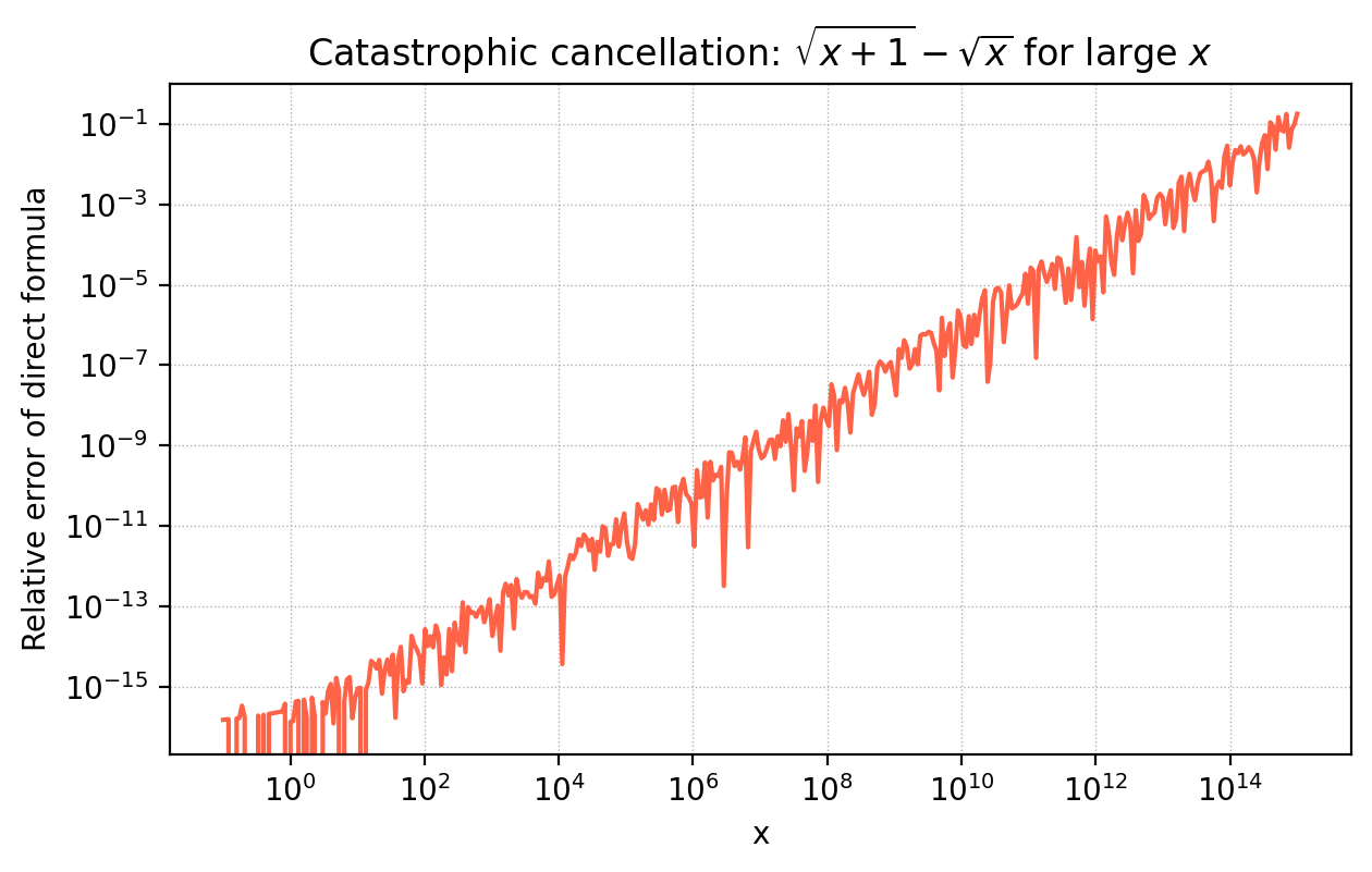
The figure illustrates this for \(\sqrt{x+1} - \sqrt{x}\). For large \(x\), the direct formula loses all precision, while the algebraically equivalent form \(1/(\sqrt{x+1}+\sqrt{x})\) is perfectly stable.
1.6 Taylor Series and Truncation Error
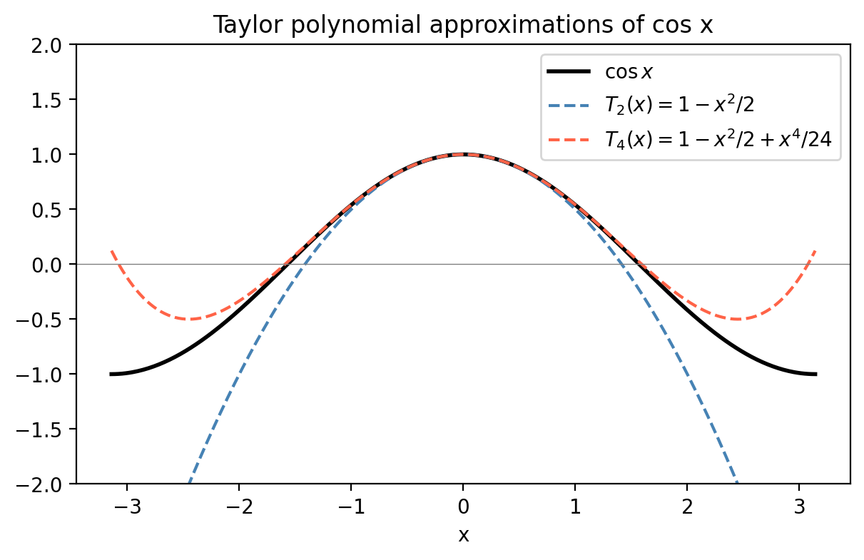
The Taylor series is the mathematical foundation of most numerical methods. Recall that if \(f\) is analytic (infinitely differentiable) near the point \(a\), then
\[f(x) = \sum_{k=0}^\infty \frac{f^{(k)}(a)}{k!}(x-a)^k.\]Truncating at the \(N\)-th term gives the \(N\)-th degree Taylor polynomial, and the error in this approximation is given by the Taylor Remainder Theorem.
This bound is not tight (it blows up near \(x = \pm\pi\)), but it confirms that the polynomial is a reasonable approximation near \(x=0\). Taylor series also let us evaluate integrals of functions with no closed form: expanding \(e^{-x^2}\) as \(1 - x^2 + x^4/2 - \cdots\) and integrating term-by-term gives \(\int_0^1 e^{-x^2}\,dx \approx 26/35 \approx 0.7429\), close to the exact value \(\frac{\sqrt\pi}{2}\,\mathrm{erf}(1) \approx 0.7468\).
Error propagation through algorithms
A subtler point: even if the truncation error in a single step is small, it can grow — sometimes exponentially — as the algorithm proceeds. As a case study, consider the recurrence \(p_n = \frac{10}{3}p_{n-1} - p_{n-2}\) started from \(p_0 = 1\), \(p_1 = 1/3\). The general solution is \(p_n = c_1(1/3)^n + c_2\cdot 3^n\); with the given initial conditions, \(c_2 = 0\). But any error \(E_0\) in computing \(p_1\) satisfies the same recurrence, giving \(E_n \approx \frac{9}{8} \cdot 3^n E_0\) — an exponentially growing error. The algorithm is unstable. An algorithm where errors grow only linearly, \(E_n \approx C_n E_0\), is stable. Stability analysis is a routine part of designing any numerical method.
1.7 Condition Number
The condition number of a problem measures how sensitive its output is to perturbations in its input. It is a property of the problem, not of any particular algorithm. Even a perfect algorithm cannot produce accurate output for an ill-conditioned problem if the input data contains any error.
For example, consider \(y = x/(1-x)\) near \(x \approx 1\). A perturbation \(\Delta x\) produces \(|\Delta y| \approx |\Delta x|/(1-x)^2\), so the relative condition number is approximately \(1/|1-x|\), which blows up as \(x \to 1\). The function is numerically useless near its singularity.
Chapter 2: Root Finding
2.1 The Problem
Given a function \(f: \mathbb{R} \to \mathbb{R}\), find \(x^*\) such that \(f(x^*) = 0\). This is one of the oldest and most fundamental problems in applied mathematics. In practice, the problem arises whenever you need to invert a function: finding the equilibrium population given a logistic growth model, finding the yield of a bond given its price, finding the resonant frequency of a circuit. The general problem has no closed-form solution — we need iterative numerical methods.
The computational target is: given \(\epsilon > 0\), find \(x^*\) such that \(|f(x^*)| < \epsilon\). We will study four methods: bisection, fixed-point iteration, Newton’s method, and the secant method. They differ in their convergence guarantees, convergence rates, and their requirements on \(f\).
2.2 Bisection
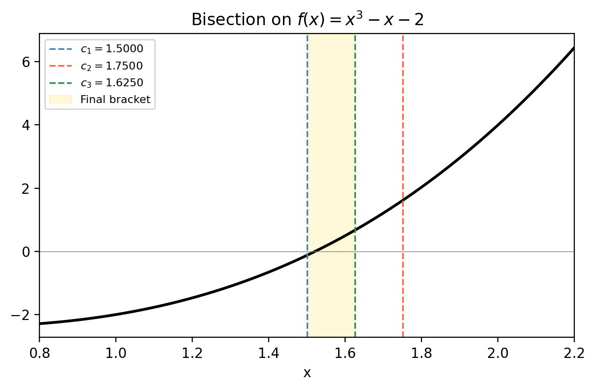
The simplest method is grounded in the Intermediate Value Theorem: if \(f\) is continuous on \([a, b]\) and \(f(a) \cdot f(b) < 0\) (the function changes sign), then there exists at least one root \(x^* \in (a, b)\).
- Compute \(c_k = (a_k + b_k)/2\).
- If \(f(a_k)f(c_k) < 0\), set \([a_{k+1}, b_{k+1}] = [a_k, c_k]\). Otherwise set \([a_{k+1}, b_{k+1}] = [c_k, b_k]\).
- Repeat until \(|b_k - a_k| < 2\epsilon\).
For \(b_0 - a_0 = 1\) and \(\epsilon = 10^{-6}\), this requires about 20 steps — very fast. Bisection is guaranteed to converge as long as \(f\) is continuous and changes sign. Its chief disadvantages are that it requires a sign-change bracket and converges only linearly (the error halves each step).
2.3 Fixed Point Iteration
A more versatile framework transforms root finding into fixed-point finding. Given \(f(x) = 0\), construct any function \(g(x) = x + H(f(x))\) where \(H(0) = 0\). Then \(f(x^*) = 0 \iff g(x^*) = x^*\): the root of \(f\) is a fixed point of \(g\). The fixed point iteration is simply
\[x_{k+1} = g(x_k).\]Whether this converges depends entirely on the choice of \(g\).
- \(g\) has a unique fixed point \(x^*\) in \([a,b]\).
- The sequence \(x_{k+1} = g(x_k)\) converges to \(x^*\) from any starting point \(x_0 \in [a,b]\).
The theorem gives a constructive existence and uniqueness result. It is an instance of the Banach fixed-point theorem, valid in any complete metric space. The proof is classical: the sequence \(\{x_k\}\) is Cauchy (each step reduces the gap by factor \(L < 1\)), so it converges; its limit must satisfy \(x^* = g(x^*)\).
A practical corollary: if \(g\) is differentiable at the fixed point, the iteration converges locally whenever \(|g'(x^*)| < 1\) and diverges whenever \(|g'(x^*)| > 1\). This is the key criterion for choosing among different reformulations of \(f(x) = 0\) as fixed-point problems.
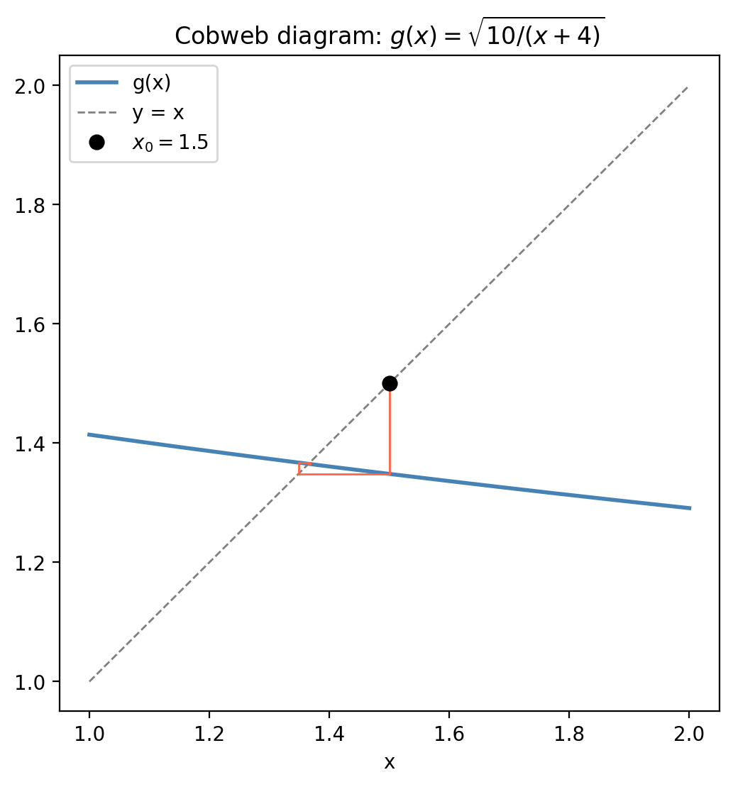
The cobweb diagram illustrates the convergence graphically: starting from \(x_0\), draw a vertical line to the graph of \(g\), then a horizontal line to \(y = x\), and repeat. When the graph of \(g\) is less steep than \(y = x\), the cobweb spirals inward to the fixed point.
2.4 Newton’s Method
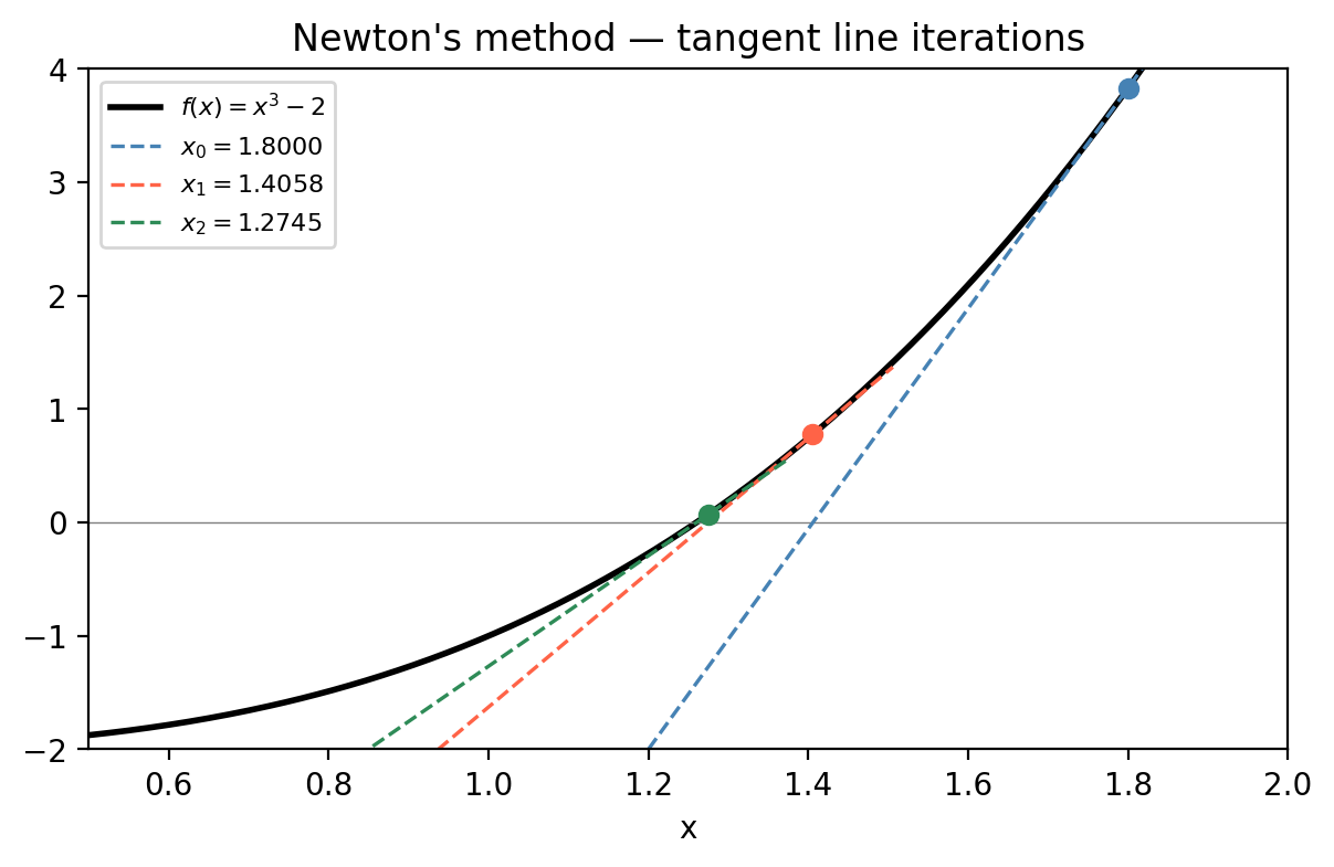
Newton’s method (independently developed by Isaac Newton (1669) and Joseph Raphson (1690)) gives a much faster convergence by using the derivative. Starting from a Taylor expansion of \(f\) around the current iterate \(x_k\):
\[f(x) \approx f(x_k) + f'(x_k)(x - x_k)\]Setting this linear approximation to zero gives the next iterate:
\[x_{k+1} = x_k - \frac{f(x_k)}{f'(x_k)}.\]Geometrically, this is the intersection of the tangent line at \((x_k, f(x_k))\) with the \(x\)-axis.
Newton’s method is a fixed-point iteration with \(g(x) = x - f(x)/f'(x)\). Computing \(g'(x^*)\) shows it vanishes at a simple root: \(g'(x^*) = f(x^*)f''(x^*)/[f'(x^*)]^2 = 0\). This means the Contraction Mapping Theorem gives local convergence, and the convergence is dramatically faster than linear.
Quadratic convergence means the number of correct decimal digits roughly doubles with each step. Starting from 1 correct digit, you get 2, then 4, then 8, etc. This is why Newton’s method typically converges in 5–10 iterations for most practical problems.
Caveat: at a multiple root \(x^*\) where both \(f(x^*) = 0\) and \(f'(x^*) = 0\), the convergence degrades to linear. In finite precision arithmetic, a near-zero denominator \(f'(x_k)\) can also cause overflow.
2.5 The Secant Method
Newton’s method requires \(f'\), which may be expensive to compute analytically or unavailable (if \(f\) is a black-box function). The secant method approximates the derivative using the last two iterates:
\[f'(x_k) \approx \frac{f(x_k) - f(x_{k-1})}{x_k - x_{k-1}}\]Substituting into Newton’s formula:
\[x_{k+1} = x_k - f(x_k) \cdot \frac{x_k - x_{k-1}}{f(x_k) - f(x_{k-1})}.\]This requires two initial guesses \(x_0\) and \(x_1\) close to the root, and one function evaluation per step (versus one evaluation of both \(f\) and \(f'\) for Newton’s).
The golden-ratio convergence rate sits between linear (\(q=1\)) and quadratic (\(q=2\)). Each secant step is cheaper than a Newton step (no derivative needed), but requires more steps to achieve the same accuracy. The practical comparison: Newton might converge in 6 iterations at cost of 6 derivative evaluations; the secant method might take 9 iterations at cost of 10 function evaluations. For expensive function evaluations, secant can win.
2.6 Convergence Rates and Comparison
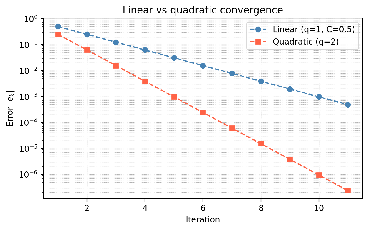
The figure makes vivid why quadratic convergence is so desirable. Starting from an error of 0.5, linear convergence needs 10 steps to reach \(5 \times 10^{-4}\); quadratic convergence reaches machine precision in about 4 steps.
| Method | Convergence rate | Requires | Guaranteed? |
|---|---|---|---|
| Bisection | Linear (factor \(1/2\)) | Sign-change bracket, \(f\) continuous | Yes |
| Fixed point | Linear or higher | ( | g’(x^*) |
| Newton’s | Quadratic | \(f \in C^2\), \(f'(x^*)\ne 0\), good \(x_0\) | Near \(x^*\) |
| Secant | Order \(\approx 1.618\) | \(f \in C^2\), good \(x_0, x_1\) | Near \(x^*\) |
In practice, a common strategy is to start with a few bisection steps to get into the neighbourhood of the root, then switch to Newton or secant for fast final convergence.
Chapter 3: Numerical Linear Algebra
3.1 The Problem
The central problem of numerical linear algebra is: given \(A \in \mathbb{R}^{n \times n}\) and \(\mathbf{b} \in \mathbb{R}^n\), find \(\mathbf{x} \in \mathbb{R}^n\) satisfying \(A\mathbf{x} = \mathbf{b}\).
\[u''(x_i) \approx \frac{u_{i+1} - 2u_i + u_{i-1}}{h^2}\]transforms the ODE into a tridiagonal linear system with coefficient matrix having diagonal entries \(2/h^2 + 1\) and off-diagonal entries \(-1/h^2\). With \(n = 10^4\) grid points, we need to solve a \(10^4 \times 10^4\) linear system efficiently.
Existence and Uniqueness
\(A\mathbf{x} = \mathbf{b}\) has a unique solution if and only if \(A\) is invertible, equivalently \(\det(A) \ne 0\), equivalently \(A\) has full rank. If \(\det(A) = 0\), the system either has infinitely many solutions (if \(\mathbf{b} \in \mathrm{Range}(A)\)) or no solution at all (if \(\mathbf{b} \notin \mathrm{Range}(A)\)). We focus on the invertible case.
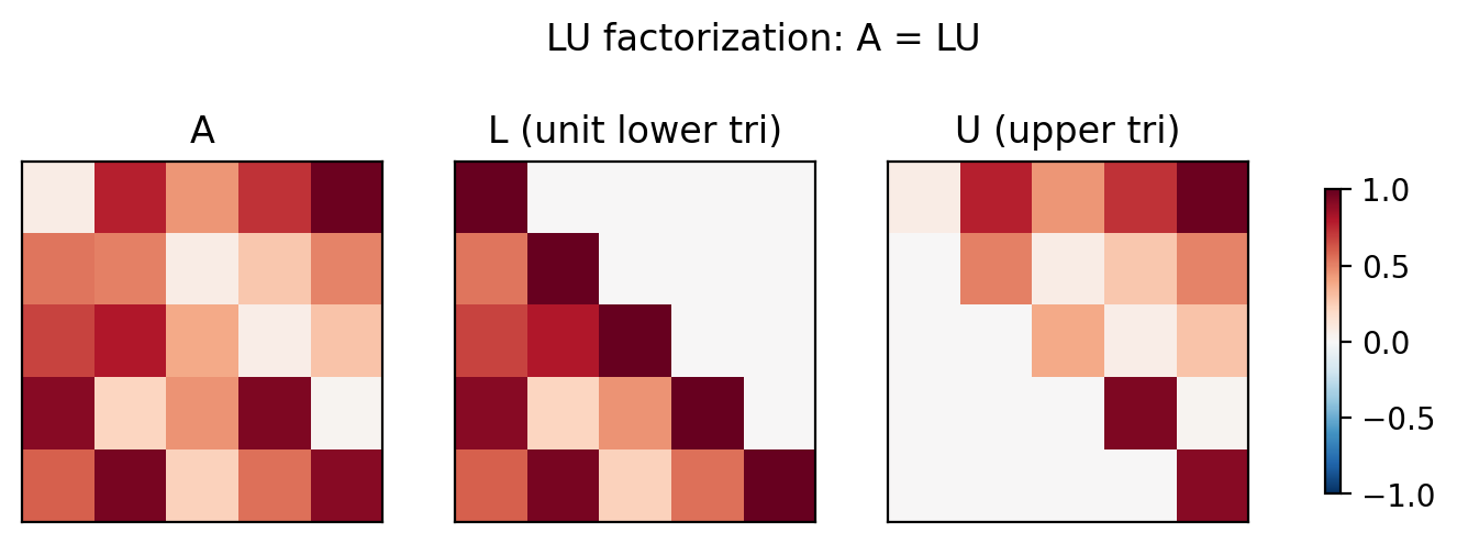
3.2 LU Factorization
Gaussian elimination (GE) is the standard algorithm for dense linear systems. Its key insight is to decompose \(A\) into a product \(A = LU\), where \(L\) is unit lower triangular (ones on the diagonal) and \(U\) is upper triangular. Once this factorisation is available, the original system \(A\mathbf{x} = \mathbf{b}\) decouples into two triangular systems:
\[L\mathbf{y} = \mathbf{b} \quad \text{(forward substitution)}, \qquad U\mathbf{x} = \mathbf{y} \quad \text{(backward substitution)}.\]Each triangular solve costs \(O(n^2)\); the LU factorisation itself costs \(O(n^3)\).
How LU is computed
\[M^{(n-1)} \cdots M^{(1)} A = U.\]Then \(L = (M^{(1)})^{-1} \cdots (M^{(n-1)})^{-1}\). The key structural insight is that these inverses are also lower-triangular, and they combine trivially: the product \((M^{(1)})^{-1}(M^{(2)})^{-1}\) is formed by simply superimposing their off-diagonal entries, without any further multiplication.
Computational cost
\[\text{Total cost} = \sum_{p=1}^{n-1} \sum_{r=p+1}^{n} (n-p) \cdot A \in O(n^3)\]where \(A\) denotes one floating point addition-multiplication. The forward and backward substitutions each cost \(O(n^2)\), so the overall cost is dominated by the factorisation.
3.3 Pivoting
Without pivoting, LU factorisation can fail or give wildly inaccurate results. The problem occurs when a pivot element \(a_{ii}^{(i)}\) (the diagonal element used as divisor for row elimination) is zero or very small, causing division by a tiny number and catastrophic amplification of rounding errors.
Partial pivoting addresses this by swapping rows at each stage to bring the largest entry in the current column to the diagonal position. This produces the factorisation \(PA = LU\), where \(P\) is a permutation matrix.
Complete pivoting searches both rows and columns for the largest entry, producing \(PAQ = LU\) with \(Q\) also a permutation matrix. It is more robust but more expensive.
In practice, LU with partial pivoting is the workhorse algorithm for dense systems. It is implemented in LAPACK as dgesv and in MATLAB as the backslash operator \. Pivoting adds only \(O(n^2)\) extra work (the row swaps) and dramatically improves numerical stability.
The algorithm with partial pivoting:
Initialize L = I, P = I, U = A
For p = 1 to n-1:
    Find index i >= p with |U(i,p)| maximal in column p
    Swap rows i and p in U, L, and P
    For each r = p+1 to n:
        m = U(r,p) / U(p,p)
        U(r, p+1:n) -= m * U(p, p+1:n)
        L(r,p) = m
3.4 Determinants from LU
The determinant is easily computed once \(PA = LU\) is available. Using the multiplicativity property \(\det(BC) = \det(B)\det(C)\) and the facts that \(\det(L) = 1\) (unit lower triangular), \(\det(U) = \prod_i u_{ii}\) (upper triangular), and \(\det(P) = \pm 1\) (depending on the parity of the permutation):
\[\det(A) = \pm \det(U) = \pm \prod_{i=1}^n u_{ii}.\]This gives \(\det(A)\) in \(O(n^3)\) (dominated by the LU factorisation), much more efficient than cofactor expansion which costs \(O(n!)\).
3.5 Matrix Norms and the Condition Number
To quantify how sensitive \(A\mathbf{x} = \mathbf{b}\) is to perturbations, we need a norm on matrices. The natural \(p\)-norm (also called the induced or operator norm) is
\[\|A\|_p = \max_{\mathbf{x} \ne \mathbf{0}} \frac{\|A\mathbf{x}\|_p}{\|\mathbf{x}\|_p}.\]This is the maximum factor by which \(A\) can stretch a vector. For the 1-norm, this equals the maximum absolute column sum; for the \(\infty\)-norm, the maximum absolute row sum; for the 2-norm, the largest singular value. Key properties include submultiplicativity: \(\|A\mathbf{x}\| \le \|A\| \cdot \|\mathbf{x}\|\) for all \(\mathbf{x}\), and \(\|AB\| \le \|A\|\cdot\|B\|\).
Now consider a perturbed system. Suppose the right-hand side changes from \(\mathbf{b}\) to \(\mathbf{b} + \Delta\mathbf{b}\), causing the solution to change from \(\mathbf{x}\) to \(\mathbf{x} + \Delta\mathbf{x}\). Since \(A(\Delta\mathbf{x}) = \Delta\mathbf{b}\):
\[\|\Delta\mathbf{x}\| = \|A^{-1}\Delta\mathbf{b}\| \le \|A^{-1}\| \cdot \|\Delta\mathbf{b}\|.\]Also, \(\|\mathbf{b}\| = \|A\mathbf{x}\| \le \|A\|\cdot\|\mathbf{x}\|\), so \(\|\mathbf{x}\| \ge \|\mathbf{b}\|/\|A\|\). Combining:
\[\frac{\|\Delta\mathbf{x}\|/\|\mathbf{x}\|}{\|\Delta\mathbf{b}\|/\|\mathbf{b}\|} \le \|A\| \cdot \|A^{-1}\|.\]For the 2-norm, \(\kappa_2(A) = \sigma_{\max}(A)/\sigma_{\min}(A)\), the ratio of largest to smallest singular values.
The derivation above handled perturbations to the right-hand side. Now consider perturbations to the coefficient matrix itself.
\[A\,\Delta\mathbf{x} = -\Delta A\,\mathbf{x} - \Delta A\,\Delta\mathbf{x}.\]\[\|\Delta\mathbf{x}\| \le \|A^{-1}\|\|\Delta A\|\|\mathbf{x}\| + \|A^{-1}\|\|\Delta A\|\|\Delta\mathbf{x}\|.\]\[\frac{\|\Delta\mathbf{x}\|/\|\mathbf{x}\|}{\|\Delta A\|/\|A\|} \le \|A^{-1}\|\|A\| = \kappa(A).\]So the same condition number \(\kappa(A)\) controls sensitivity to both right-hand-side and matrix perturbations. A system is ill-conditioned if and only if small relative changes in either \(\mathbf{b}\) or \(A\) can produce large relative changes in the solution \(\mathbf{x}\).
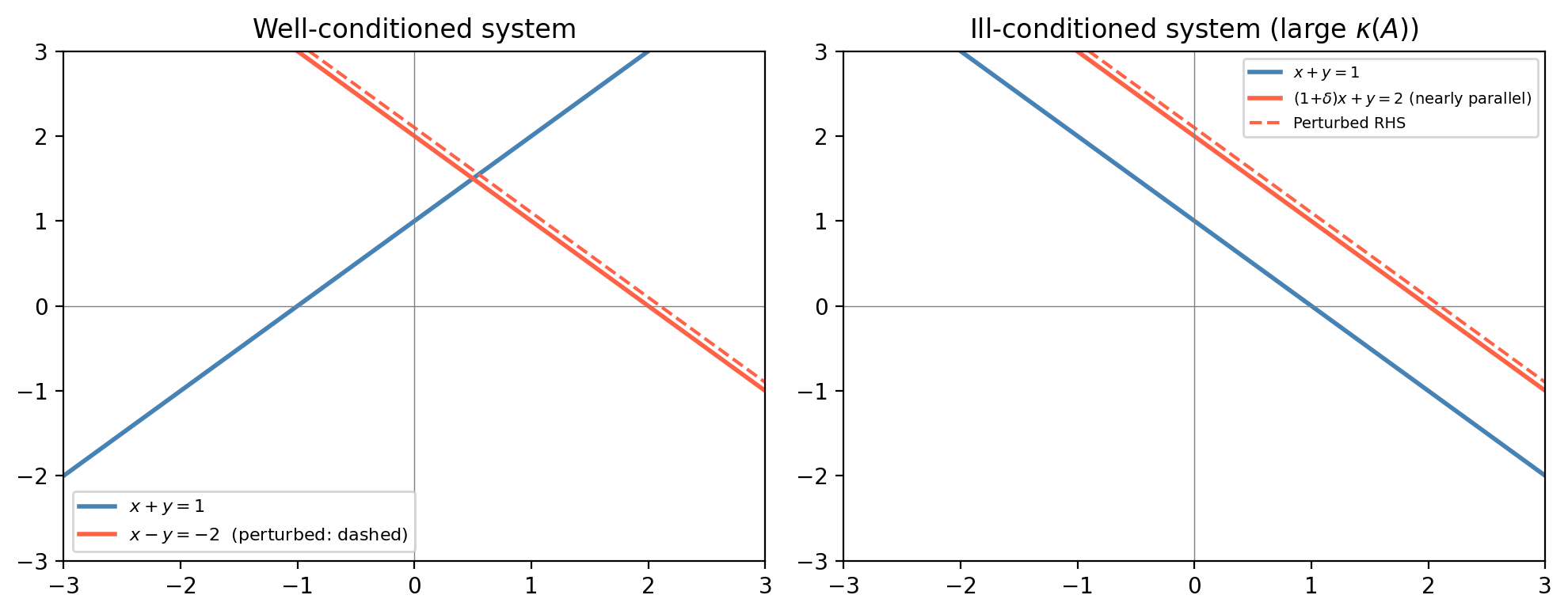
The geometric intuition is clear: nearly parallel constraint lines define an intersection point whose position is highly sensitive to small tilts in either line. A large condition number corresponds geometrically to near-linear dependence of the rows.
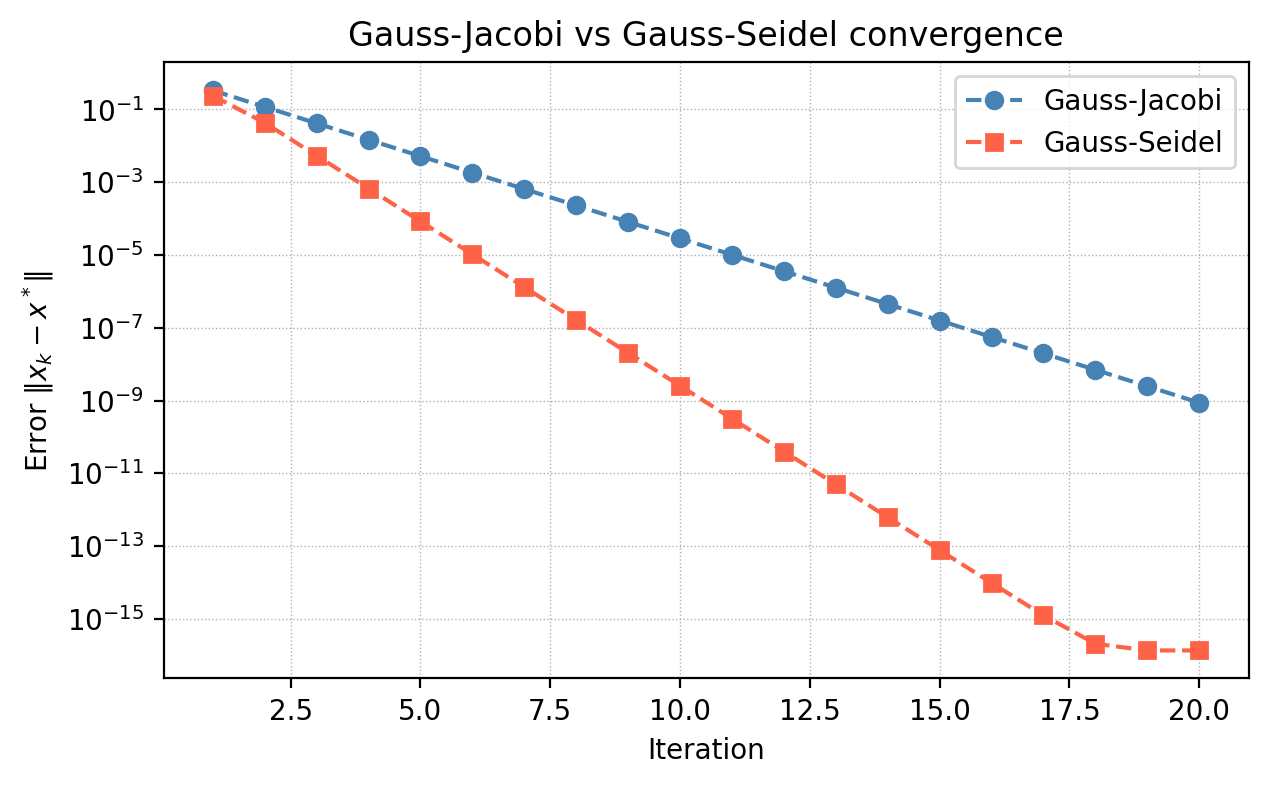
3.6 Iterative Methods: Gauss-Jacobi and Gauss-Seidel
Direct methods (LU factorisation) solve \(A\mathbf{x} = \mathbf{b}\) exactly in \(O(n^3)\) operations. For large sparse matrices (few nonzero entries per row), this is wasteful: LU fill-in creates dense factors even from sparse matrices. When \(A\) is sparse with \(O(n)\) nonzeros and well-conditioned, iterative methods can solve the system much faster.
\[\mathbf{x}_k = M^{-1}(N\mathbf{x}_{k-1} + \mathbf{b}) = M^{-1}(M - A)\mathbf{x}_{k-1} + M^{-1}\mathbf{b}.\]This is a fixed-point iteration. If it converges, the limit \(\mathbf{x}^*\) satisfies \(\mathbf{x}^* = M^{-1}(M-A)\mathbf{x}^* + M^{-1}\mathbf{b}\), i.e. \(A\mathbf{x}^* = \mathbf{b}\).
\[x_k^{(i)} = \frac{1}{a_{ii}}\left(b_i - \sum_{j \ne i} a_{ij} x_{k-1}^{(j)}\right).\]\[x_k^{(i)} = \frac{1}{a_{ii}}\left(b_i - \sum_{j < i} a_{ij} x_k^{(j)} - \sum_{j > i} a_{ij} x_{k-1}^{(j)}\right).\]Gauss-Seidel typically converges about twice as fast as Gauss-Jacobi because it uses more up-to-date information. Each iteration of either method costs only \(O(n)\) for sparse \(A\), versus \(O(n^2)\) for one solve with the dense triangular factors from LU.
Chapter 4: Polynomial Interpolation
4.1 The Interpolation Problem
Given a set of distinct nodes \(\{x_0, x_1, \ldots, x_n\}\) and corresponding function values \(\{f_0, f_1, \ldots, f_n\}\), find a continuous function \(p\) such that \(p(x_i) = f_i\) for all \(i\). This is called interpolation. It arises constantly in practice: measuring a physical quantity at discrete time points and needing to estimate it at intermediate times; tabulating a function and needing smooth values between table entries.
A foundational reassurance is given by the Weierstrass theorem:
This theorem guarantees the existence of good polynomial approximations, but it does not tell us how to find them efficiently. That is the job of the next few sections. We restrict attention to polynomials, which are the simplest class of smooth functions: easy to evaluate, differentiate, and integrate.
4.2 The Monomial (Vandermonde) Approach
The most natural polynomial basis is \(\{1, x, x^2, \ldots, x^n\}\). Writing \(p(x) = \sum_{i=0}^n \alpha_i x^i\) and applying the interpolation condition at each node gives the linear system
\[\begin{bmatrix} 1 & x_0 & x_0^2 & \cdots & x_0^n \\ 1 & x_1 & x_1^2 & \cdots & x_1^n \\ \vdots \\ 1 & x_n & x_n^2 & \cdots & x_n^n \end{bmatrix} \begin{bmatrix} \alpha_0 \\ \vdots \\ \alpha_n \end{bmatrix} = \begin{bmatrix} f_0 \\ \vdots \\ f_n \end{bmatrix}.\]The coefficient matrix is the Vandermonde matrix \(V\). Its determinant is \(\det(V) = \prod_{0 \le i < j \le n} (x_j - x_i) \ne 0\) when all nodes are distinct, proving that the interpolating polynomial exists and is unique. Uniqueness holds generally:
Proof sketch: If \(p\) and \(q\) both interpolate the data, then \(r = p - q\) is a polynomial of degree \(\le n\) with \(n+1\) roots. By the fundamental theorem of algebra, \(r \equiv 0\), so \(p = q\). \(\square\)
The Vandermonde approach has two serious drawbacks. For large \(n\), powers \(x_i^n\) can overflow or underflow; and the Vandermonde matrix is notoriously ill-conditioned, making the linear solve inaccurate even when solutions exist. We need a better approach.
4.3 Lagrange Interpolation
The Lagrange basis circumvents the Vandermonde system entirely by constructing the interpolating polynomial directly. For each node \(x_i\), define the Lagrange basis polynomial:
\[L_i(x) = \prod_{\substack{k=0 \\ k \ne i}}^n \frac{x - x_k}{x_i - x_k}.\]By construction, \(L_i(x_j) = \delta_{ij}\) (Kronecker delta): \(L_i\) equals 1 at \(x_i\) and 0 at all other nodes. The interpolating polynomial is then
\[p(x) = \sum_{i=0}^n f_i L_i(x).\]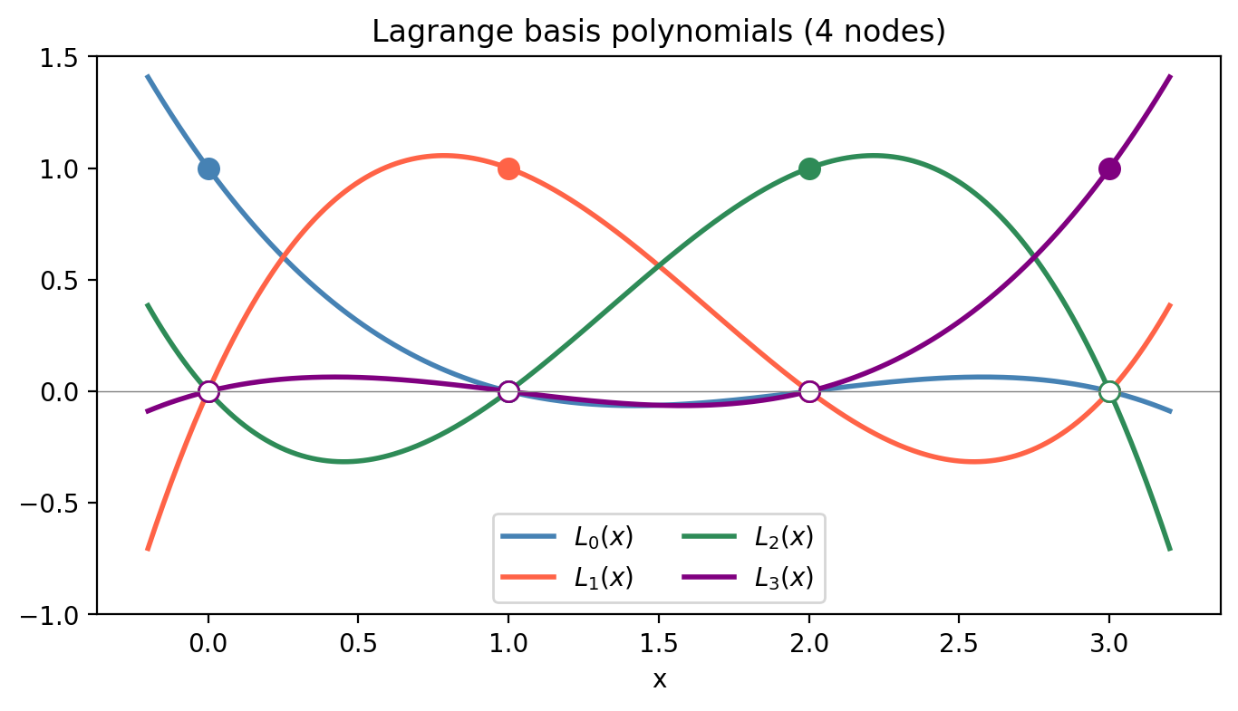
Each \(L_i\) has degree \(n\), so \(p\) has degree \(\le n\). Evaluating \(p\) at a new point costs \(O(n^2)\): forming each \(L_i\) requires \(O(n)\) multiplications, and there are \(n+1\) basis functions.
4.4 Barycentric Form and Efficient Updates
\[\ell'(x_i) = \prod_{\substack{j=0 \\ j \ne i}}^n (x_i - x_j).\]Then each Lagrange basis polynomial can be written \(L_i(x) = \ell(x) \cdot w_i/(x - x_i)\), and the interpolant becomes
\[p(x) = \ell(x) \sum_{i=0}^n \frac{w_i}{x - x_i} f_i.\]Since \(\sum_{i=0}^n L_i(x) = 1\), we have \(\ell(x) \sum_{i=0}^n w_i/(x-x_i) = 1\), giving the barycentric formula:
\[p(x) = \frac{\displaystyle\sum_{i=0}^n \dfrac{w_i}{x - x_i} f_i}{\displaystyle\sum_{i=0}^n \dfrac{w_i}{x - x_i}}.\]This form is numerically superior: evaluating at a point costs only \(O(n)\). Adding a new node \(x_{n+1}\) requires only updating each \(w_i\) by dividing by \((x_i - x_{n+1})\), and computing the new weight \(w_{n+1} = 1/\prod_{j=0}^n (x_{n+1} - x_j)\) — an \(O(n)\) operation.
4.5 Hermite Interpolation
Sometimes we know not just function values but also derivative values at the nodes. The Hermite interpolation problem seeks a polynomial \(H\) satisfying both \(H(x_i) = f_i\) and \(H'(x_i) = f_i'\) at each of \(n+1\) nodes. Since we impose \(2(n+1)\) conditions, \(H\) must have degree at most \(2n+1\).
\[H(x) = \sum_{i=0}^n f_i\bigl(1 - 2(x-x_i)L_i'(x_i)\bigr)L_i^2(x) + \sum_{i=0}^n f_i'(x - x_i)L_i^2(x).\]One can verify that this polynomial satisfies all the interpolation and derivative conditions. Hermite interpolation at two points (a single interval) produces the cubic Hermite polynomial, which is the local building block of cubic splines.
4.6 Issues with High-Degree Polynomial Interpolation
As the number of nodes \(n\) grows, polynomial interpolation can behave unexpectedly badly. The most famous example is Runge’s phenomenon: for the function \(f(x) = 1/(1+25x^2)\) on \([-1,1]\), the interpolating polynomial on equally-spaced nodes oscillates wildly near the endpoints as \(n\) increases, despite the function being smooth.
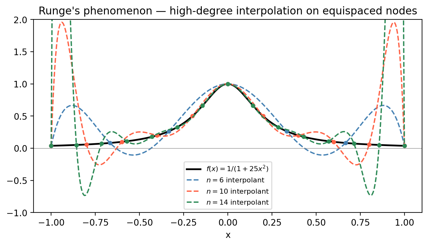
With Chebyshev nodes, the interpolation error is nearly equioscillated across the interval, and the Lebesgue constant (a measure of the worst-case amplification factor) grows only logarithmically with \(n\), rather than exponentially.
4.7 Piecewise Polynomial and Spline Interpolation
Rather than using a single high-degree polynomial, we can use piecewise polynomials: low-degree polynomials on each subinterval \([x_{i-1}, x_i]\), glued together with smoothness conditions.
Piecewise linear interpolation connects the data points by straight-line segments. It is globally continuous but not differentiable at the nodes, which is unacceptable when smooth derivatives are needed (e.g., for ODEs).
Cubic spline interpolation uses a cubic polynomial \(S_k(x) = a_k + b_k(x-x_k) + c_k(x-x_k)^2 + d_k(x-x_k)^3\) on each interval \([x_{k-1}, x_k]\), subject to:
- Interpolation: \(S_k(x_k) = f_k\) (matches the data values)
- Continuity: \(S_k(x_{k-1}) = S_{k-1}(x_{k-1})\) (adjacent pieces agree)
- 1st smoothness: \(S_k'(x_{k-1}) = S_{k-1}'(x_{k-1})\) (continuous first derivatives)
- 2nd smoothness: \(S_k''(x_{k-1}) = S_{k-1}''(x_{k-1})\) (continuous second derivatives)
These conditions, together with two boundary conditions (most commonly the free/natural cubic spline: \(S_1''(x_0) = 0\) and \(S_n''(x_n) = 0\)), give a unique solution. The resulting linear system for the coefficients is tridiagonal and can be solved in \(O(n)\) with Gaussian elimination.
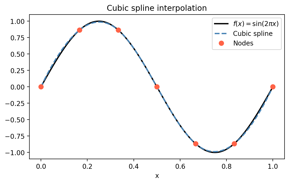
The cubic spline achieves \(C^2\) smoothness (continuous up to second derivative) across all nodes while fitting the data exactly. This makes it the standard tool for smooth curve fitting in computer graphics, CAD, and scientific computing.
Chapter 5: Numerical Integration
5.1 The Problem of Quadrature
Numerical integration — or quadrature — approximates \(\int_a^b f(x)\,dx\) when the integral cannot be computed in closed form or when \(f\) is available only at discrete points. Examples: \(\int_0^1 e^{-x^2}dx\) (no elementary antiderivative), integrals of measured data, or integrals appearing inside larger numerical algorithms.
\[Q(f) = \sum_{i=0}^n w_i f(x_i) \approx \int_a^b f(x)\,dx\]where \(\{x_i\}\) are the quadrature nodes and \(\{w_i\}\) are the quadrature weights. The methods differ in how the nodes and weights are chosen. If the nodes are derived from polynomial interpolation, the rule is called an interpolatory rule; if they are equispaced, it is a Newton-Cotes rule.
The condition of the integration problem is gentle: \(|I(f) - I(\hat f)| \le (b-a)\|f - \hat f\|_\infty\), so small uniform perturbations in \(f\) cause proportionally small errors in the integral.
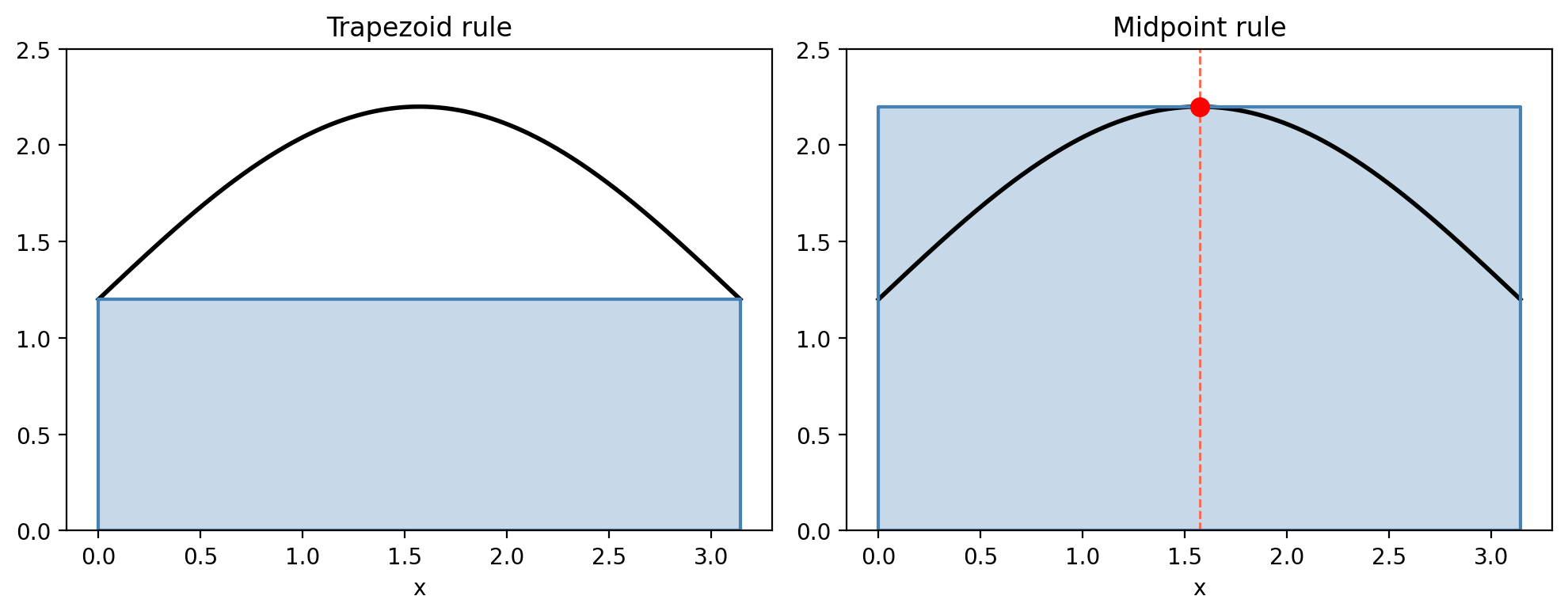
5.2 The Trapezoid Rule
The simplest interpolatory rule uses a degree-1 polynomial (a line) on \([a,b]\). Using the Lagrange interpolating polynomial through \(f(a)\) and \(f(b)\):
\[\int_a^b f(x)\,dx \approx \int_a^b \left(\frac{x-b}{a-b}f(a) + \frac{x-a}{b-a}f(b)\right)dx = \frac{b-a}{2}\bigl[f(a) + f(b)\bigr].\]\[E_T(f) = -\frac{(b-a)^3}{12}f''(\xi)\]for some \(\xi \in (a,b)\), showing that the trapezoid rule is exact for linear functions.
5.3 The Midpoint Rule
\[M(f) = (b-a)f\!\left(\frac{a+b}{2}\right).\]The truncation error is \(E_M(f) = \frac{(b-a)^3}{24}f''(m)\), exactly half the trapezoid error in magnitude. Both rules are exact for degree-1 polynomials; neither is exact for degree-2.
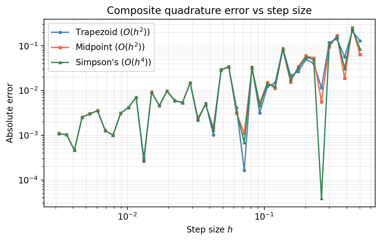
5.4 Composite Rules
On a single interval, the error of order \((b-a)^3\) is fine for small \(b-a\). For large intervals, we partition \([a,b]\) into \(n\) equal subintervals of width \(h = (b-a)/n\) and apply the basic rule on each subinterval.
\[CT(f) = \frac{h}{2}\bigl[f(x_0) + 2f(x_1) + 2f(x_2) + \cdots + 2f(x_{n-1}) + f(x_n)\bigr],\]with error \(|I(f) - CT(f)| \le \frac{(b-a)h^2}{12}\max_{[a,b]}|f''|\). Note the error is \(O(h^2)\): halving the step size reduces the error by a factor of 4.
Composite Midpoint Rule: analogously, with error \(|I(f) - CM(f)| \le \frac{(b-a)h^2}{24}\max|f''|\). Both composite rules cost \(O(n) = O((b-a)/h)\) function evaluations.
5.5 Simpson’s Rule
\[\int_a^b f(x)\,dx \approx \frac{b-a}{6}\left[f(a) + 4f\!\left(\frac{a+b}{2}\right) + f(b)\right].\]A striking fact: although Simpson’s rule uses a degree-2 polynomial, it is exact for degree-3 polynomials. This is because the linear term in the error cancels by symmetry. This phenomenon — a rule being more accurate than expected from the degree of its polynomial — is called super-convergence.
The order of accuracy of a quadrature rule is the largest \(p\) such that the rule integrates all polynomials of degree \(\le p\) exactly. For Newton-Cotes rules with \(n\) points: if \(n\) is odd, the order is \(n\); if \(n\) is even, the order is \(n+1\) (one extra order from the super-convergence).
| Rule | Function evaluations | Order of accuracy |
|---|---|---|
| Midpoint | 1 | 2 |
| Trapezoid | 2 | 2 |
| Simpson’s | 3 | 4 |
The composite Simpson’s rule has error \(O(h^4)\), far better than \(O(h^2)\) for the same number of function evaluations.
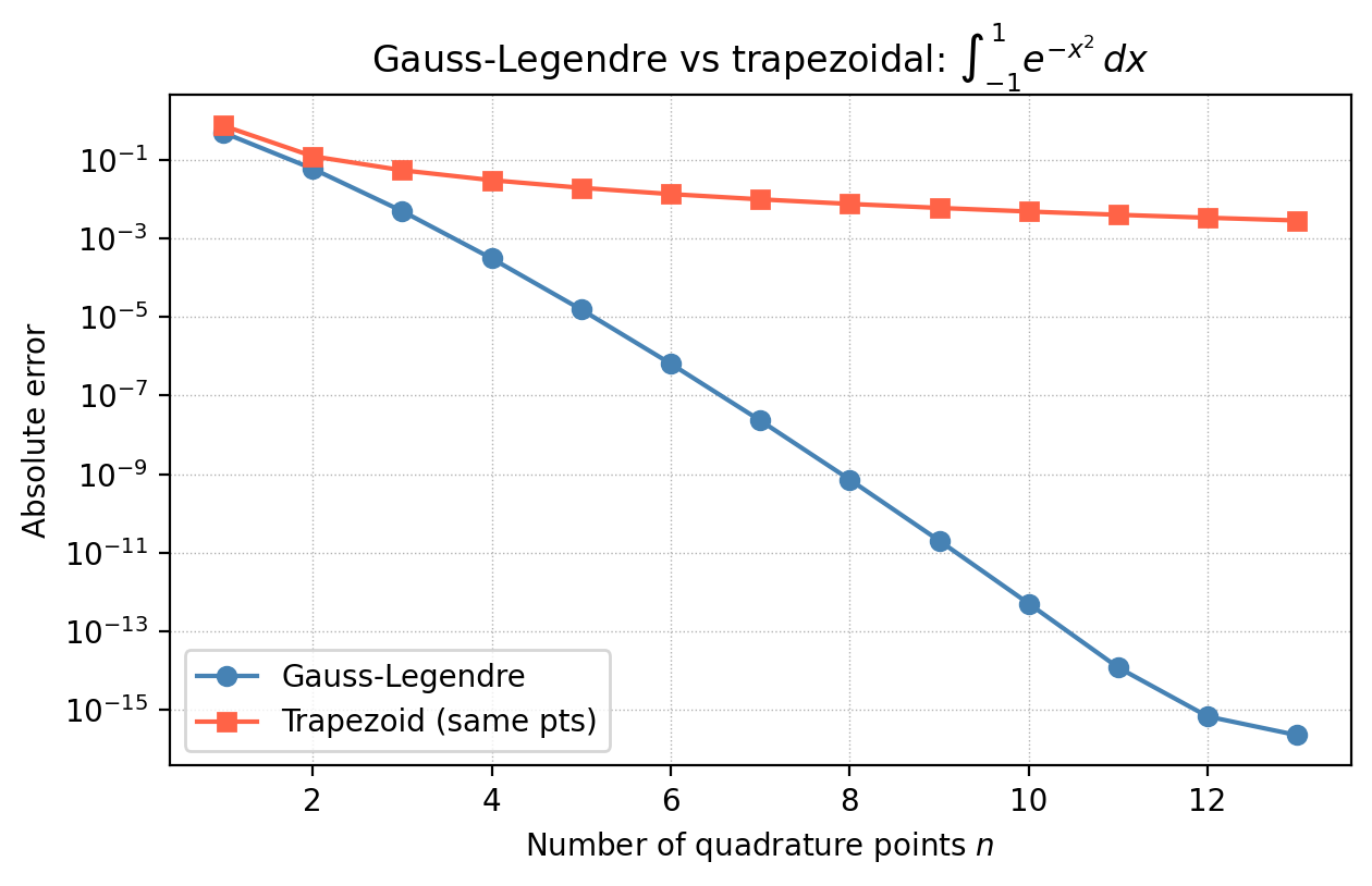
5.6 Gaussian Quadrature
Newton-Cotes rules fix the nodes (equispaced) and optimise the weights. What if we optimise both nodes and weights? This is the idea behind Gaussian quadrature, and the gain is remarkable.
For an \(n\)-point rule on \([-1, 1]\), Gaussian quadrature chooses nodes and weights to make the rule exact for all polynomials of degree \(\le 2n-1\) — roughly twice the order of Newton-Cotes with the same number of points.
The positivity of the weights is significant: it ensures stability. For Newton-Cotes rules with \(n \ge 11\), some weights become negative, which can cause severe cancellation errors when applied to non-smooth functions.
\[R_n(f) = \frac{2^{2n+1}(n!)^4}{(2n+1)[(2n)!]^3}\,f^{(2n)}(\xi), \quad \xi \in [-1,1].\]For analytic functions (smooth everywhere), the Gauss-Legendre error decreases exponentially in \(n\) — spectral convergence — whereas Newton-Cotes converges only polynomially. To integrate over a general interval \([a,b]\), change variables: let \(t = (2x - a - b)/(b-a)\), so \(x = ((b-a)t + a + b)/2\) and \(dx = (b-a)/2\,dt\).
5.7 Special Integration Problems
Tabular data: if \(f\) is known only at measured points \(\{(x_i, f_i)\}\) (not necessarily equispaced), apply the composite trapezoid rule using the given nodes, or fit a cubic spline and integrate it analytically.
Improper integrals: for \(\int_a^\infty f(x)\,dx\), choose a sufficiently large cut-off \(c\) such that \(\int_c^\infty f\,dx\) is negligible, and integrate \(\int_a^c f\,dx\) numerically. For singularities at the endpoint (e.g., \(\int_0^{\pi/2}\cos x/\sqrt{x}\,dx\)), use a substitution to remove the singularity: letting \(x = t^2\) gives \(2\int_0^{\sqrt{\pi/2}}\cos(t^2)\,dt\), which is smooth.
Double integrals: treat \(\int_a^b\bigl(\int_c^d f(x,y)\,dx\bigr)dy\) as a one-dimensional integral of the inner function \(g(y) = \int_c^d f(x,y)\,dx\), applying quadrature to each dimension in turn. For a 2D rule with \(n\) points per dimension, the cost is \(O(n^2)\); in \(d\) dimensions it is \(O(n^d)\) — the curse of dimensionality that makes classical quadrature expensive in high dimensions.
Chapter 6: The Discrete Fourier Transform
6.1 From Continuous to Discrete: Motivation
Many signals in the real world — audio, seismic measurements, medical images — are periodic or nearly periodic, and it is natural to decompose them into sinusoidal components. The Fourier series does this for continuous periodic functions. But in practice, we have only discrete samples \(f[0], f[1], \ldots, f[N-1]\), not a continuous function. The Discrete Fourier Transform (DFT) is the natural analogue: it expresses a discrete, periodic signal in terms of discrete frequencies.
The FFT (Fast Fourier Transform), a divide-and-conquer algorithm for computing the DFT, is one of the most important algorithms of the 20th century. James Cooley and John Tukey published it in 1965 (though Gauss had discovered it in 1805, unpublished), and it reduced the cost of computing the DFT from \(O(N^2)\) to \(O(N\log N)\). It powers MP3 compression, medical imaging, telecommunications, and countless other technologies.
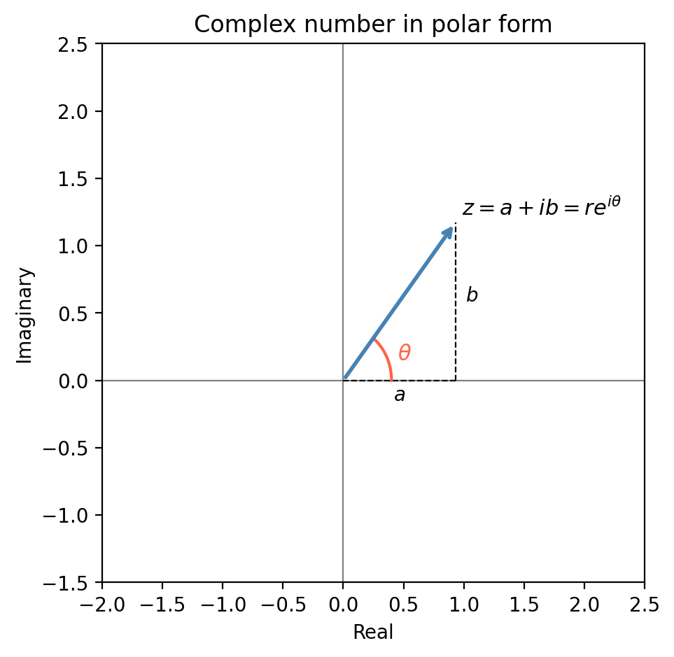
6.2 Complex Numbers and Euler’s Formula
The natural language of Fourier analysis is complex numbers. A complex number \(z = a + ib\) has real part \(\mathrm{Re}(z) = a\), imaginary part \(\mathrm{Im}(z) = b\), modulus \(|z| = \sqrt{a^2+b^2}\), and complex conjugate \(\bar z = a - ib\). In polar form, \(z = re^{i\theta}\) where \(r = |z|\) and \(\theta = \arctan(b/a)\).
This extraordinary formula connects the exponential function to trigonometry. It follows by comparing the Taylor series of \(e^{i\theta}\), \(\cos\theta\), and \(\sin\theta\) term by term. Euler’s formula implies \(e^{i\pi} + 1 = 0\) (Euler’s identity), which links the five most important constants in mathematics. For our purposes, it means that sinusoidal oscillations can be written compactly as real and imaginary parts of complex exponentials: \(\cos\theta = \mathrm{Re}(e^{i\theta})\), \(\sin\theta = \mathrm{Im}(e^{i\theta})\).
6.3 Continuous Fourier Series
\[f(t) = \frac{a_0}{2} + \sum_{k=1}^\infty \left[a_k \cos\!\left(\frac{2\pi k}{T}t\right) + b_k \sin\!\left(\frac{2\pi k}{T}t\right)\right]\]\[a_k = \frac{2}{T}\int_0^T f(t)\cos\!\left(\frac{2\pi k}{T}t\right)dt, \quad b_k = \frac{2}{T}\int_0^T f(t)\sin\!\left(\frac{2\pi k}{T}t\right)dt.\]Why do these formulas work? The key is orthogonality: integrating the product of any two distinct basis functions \(\cos(kt)\) and \(\cos(jt)\) (or any mix) over a full period gives zero. This means the Fourier basis \(\{1, \cos(kt), \sin(kt)\}_{k=1}^\infty\) behaves like an orthogonal coordinate system in the function space \(L^2[-\pi, \pi]\) — projecting \(f\) onto each basis vector (by integration) extracts the corresponding coefficient independently.
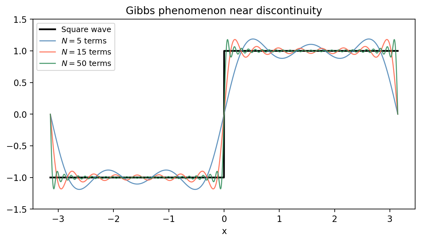
The class \(L^2[-\pi, \pi]\) is very large — it includes discontinuous functions, which the Fourier series can approximate in mean-square. However, pointwise convergence at discontinuities exhibits the Gibbs phenomenon: the partial sums overshoot by about 9% near a jump discontinuity, regardless of how many terms are taken.
The last integral is evaluated by integration by parts: \(\int x\sin(ax)\,dx = -x\cos(ax)/a + \sin(ax)/a^2\). Therefore
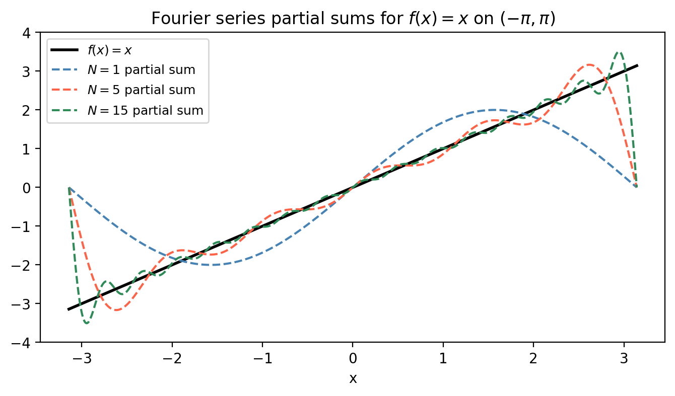
\[f(x) \sim \frac{4}{\pi}\sum_{k=1}^\infty \frac{(-1)^{k+1}}{k}\sin\!\left(\frac{k\pi x}{2}\right).\]As the figure shows, the partial sums converge rapidly away from the endpoints, and the boundary jump causes mild Gibbs-like ringing.
Odd and even symmetry. Computing Fourier coefficients from scratch for every function would be tedious. Two symmetry shortcuts save work: if \(f\) is an odd function (\(f(-t) = -f(t)\)), then all cosine coefficients vanish — \(a_k = 0\) for all \(k\) — because the integrand \(f(t)\cos(kt)\) is odd over a symmetric interval. Conversely, if \(f\) is an even function (\(f(-t) = f(t)\)), then all sine coefficients vanish — \(b_k = 0\) — since \(f(t)\sin(kt)\) is odd. The example above (\(f(x)=x\) is odd) confirms \(a_k = 0\) for all \(k\).
\[f(t) = \sum_{k=-\infty}^\infty c_k e^{ikt}, \quad c_k = \frac{1}{2\pi}\int_{-\pi}^\pi f(t)e^{-ikt}\,dt.\]The real and complex coefficients are related by \(a_k = -2\mathrm{Re}(c_k)\), \(b_k = -2\mathrm{Im}(c_k)\).
6.4 The Discrete Fourier Transform
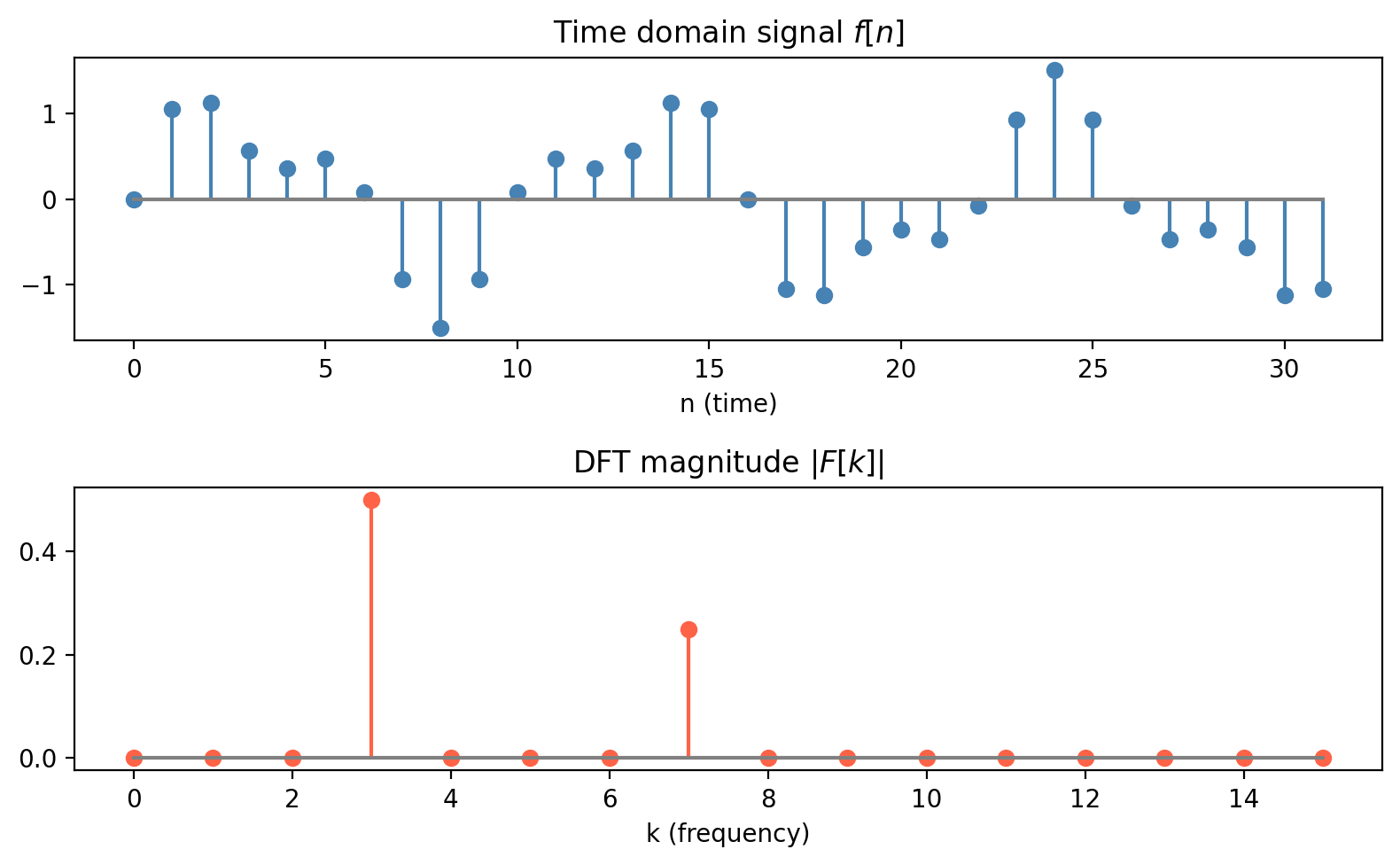
Now suppose we have only \(N\) equally-spaced samples \(f[0], f[1], \ldots, f[N-1]\) of an \(N\)-periodic discrete signal. The Discrete Fourier Transform is:
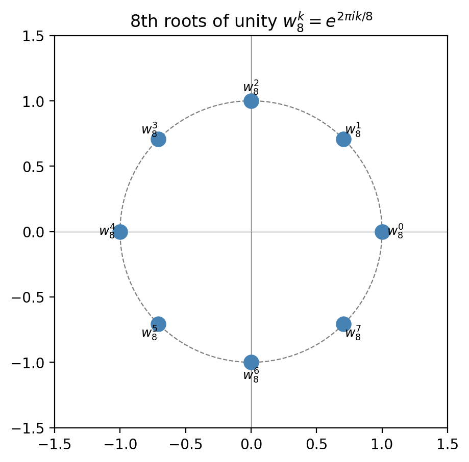
\[\mathcal{F}[k] = \frac{1}{N}\sum_{n=0}^{N-1} f[n]\,\omega_N^{-kn}, \quad k = 0, 1, \ldots, N-1,\]where \(\omega_N = e^{2\pi i/N}\) is the primitive \(N\)-th root of unity. The collection \(\{1, \omega_N, \omega_N^2, \ldots, \omega_N^{N-1}\}\) are all the \(N\)-th roots of unity, equally spaced around the unit circle.
In matrix form, \(W\mathbf{f}/N = \mathbf{F}\) where \(W\) is the DFT matrix with entries \(W_{kn} = \omega_N^{-kn}\). The inverse satisfies \(W^{-1} = N\overline{W}\), i.e. the DFT matrix is (up to scaling) unitary.
The DFT connects to the continuous Fourier series: for a function sampled at \(N\) equispaced points, the DFT coefficients approximate the Fourier series coefficients, with aliasing errors for frequencies above the Nyquist limit \(N/2\).
Aliasing and the Nyquist-Shannon Theorem: if the signal contains frequency components at \(f > N/(2T)\), those components are indistinguishable from lower-frequency aliases in the sampled signal. To avoid aliasing, you must sample at least twice the maximum frequency present in the signal.
For real time signals, \(\mathcal{F}[-k] = \overline{\mathcal{F}[k]}\) (the spectrum is Hermitian symmetric), so only frequencies \(k = 0, 1, \ldots, N/2\) contain independent information.
6.5 The Fast Fourier Transform
Naively computing all \(N\) DFT coefficients costs \(O(N^2)\): each \(\mathcal{F}[k]\) is a sum of \(N\) terms, and there are \(N\) coefficients. For \(N = 10^6\), this requires \(10^{12}\) operations — about 1000 seconds on a modern CPU. The FFT reduces this to \(O(N\log N)\) — about 0.02 seconds for the same \(N\).
The key insight is divide-and-conquer. Split the sum into even-indexed and odd-indexed terms:
\[\mathcal{F}[k] = \frac{1}{N}\sum_{n=0}^{N-1}f[n]\omega_N^{-kn} = \frac{1}{N}\left(\sum_{n=0}^{N/2-1}f[n]\omega_N^{-kn} + \sum_{n=0}^{N/2-1}f\!\left[n+\frac{N}{2}\right]\omega_N^{-k(n+N/2)}\right).\]Using \(\omega_N^{-kN/2} = (-1)^k\):
\[\mathcal{F}[k] = \frac{1}{N}\sum_{n=0}^{N/2-1}\left(f[n] + (-1)^k f\!\left[n+\frac{N}{2}\right]\right)\omega_N^{-kn}.\]For even \(k = 2\ell\): \(\mathcal{F}[2\ell] = \frac{1}{2}\,\mathrm{DFT}_{N/2}\!\left\{f[n] + f\!\left[n+\frac{N}{2}\right]\right\}_\ell.\)
For odd \(k = 2\ell+1\): \(\mathcal{F}[2\ell+1] = \frac{1}{2}\,\mathrm{DFT}_{N/2}\!\left\{\left(f[n] - f\!\left[n+\frac{N}{2}\right]\right)\omega_N^{-n}\right\}_\ell.\)
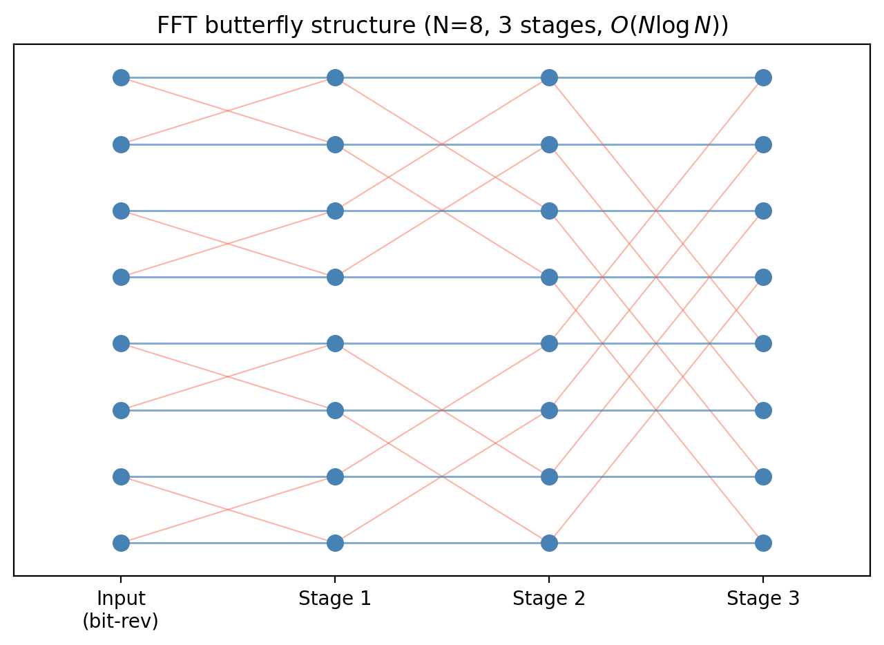
Both halves are \(N/2\)-point DFTs. If \(N = 2^m\), we can recurse all the way down to 1-point DFTs (trivial), performing \(m = \log_2 N\) levels of splitting. Each level costs \(O(N)\) operations (the additions and the twiddle-factor multiplications by \(\omega_N^{-n}\)), giving total cost \(O(N\log_2 N)\).
When \(N\) is not a power of 2, several strategies exist. The Cooley-Tukey mixed-radix algorithm works when \(N\) has small prime factors (e.g., \(N = 2^a 3^b 5^c\)). Alternatively, zero-padding extends the signal to the next power of 2 by appending zeros; this changes the DFT slightly but allows the power-of-two FFT to run.
6.6 Application: Polynomial Multiplication
The FFT enables a surprising speed-up in polynomial arithmetic. Given two polynomials \(p(x)\) and \(q(x)\) of degree \(n\), their product \(r(x) = p(x)q(x)\) has degree \(2n\) and computing its coefficients directly by convolution costs \(O(n^2)\).
The key observation: polynomial multiplication in coefficient space is equivalent to pointwise multiplication in value space. If we evaluate \(p\) and \(q\) at \(2n+1\) points, form \(r(x_k) = p(x_k)q(x_k)\) pointwise, and then interpolate back to get the coefficients of \(r\), we have computed the product.
Evaluating a degree-\(n\) polynomial at \(N = 2n\) points via the Vandermonde system is \(O(N^2)\). But if the evaluation points are chosen to be the \(N\)-th roots of unity, the evaluation matrix becomes the DFT matrix, and we can evaluate all \(N\) points in \(O(N\log N)\) using the FFT. The algorithm:
- Compute \(\hat p = \mathrm{DFT}(\mathbf{p})\) and \(\hat q = \mathrm{DFT}(\mathbf{q})\) — each \(O(N\log N)\).
- Form \(\hat r[k] = \hat p[k] \cdot \hat q[k]\) — \(O(N)\).
- Recover \(\mathbf{r} = \mathrm{IDFT}(\hat r)\) — \(O(N\log N)\).
Total: \(O(N\log N)\) instead of \(O(N^2)\). This is the algorithm used in modern computer algebra systems for large polynomial and integer multiplication (Schönhage-Strassen).
Appendix: Summary of Key Results
| Topic | Key result | Cost |
|---|---|---|
| Bisection | Halves bracket each step; \(k > \log_2((b-a)/\epsilon)\) steps needed | \(O(k)\) function evals |
| Newton’s method | Quadratic convergence near simple root | 1 eval of \(f, f'\) per step |
| LU factorisation | \(PA = LU\); solves \(Ax = b\) in \(O(n^3)\) | \(O(n^3)\) total |
| Condition number | \(\kappa(A) = \|A\|\|A^{-1}\|\); loses \(\log_{10}\kappa\) digits | — |
| Gauss-Jacobi/Seidel | \(O(n)\) per iteration for sparse \(A\); converges if \(A\) diag. dominant | \(O(n)\)/iteration |
| Lagrange interpolation | Unique degree-\(\le n\) polynomial through \(n+1\) points | \(O(n^2)\) to evaluate |
| Barycentric form | Same interpolant, \(O(n)\) per evaluation | \(O(n)\) per eval |
| Cubic spline | \(C^2\) piecewise cubic through \(n+1\) data points | \(O(n)\) to set up |
| Composite trapezoid | Error \(O(h^2)\) | \(O(n)\) evals |
| Composite Simpson’s | Error \(O(h^4)\) | \(O(n)\) evals |
| Gauss-Legendre | Exact for degree \(\le 2n-1\); spectral for analytic \(f\) | \(n\) evals |
| DFT | Converts \(N\) samples to \(N\) frequency components | \(O(N^2)\) naive |
| FFT | Same as DFT, divide-and-conquer | \(O(N\log N)\) |
