STAT 231: Statistics
Estimated study time: 50 minutes
Table of contents
Chapter 1: Introduction to Statistical Sciences
1.1 Empirical Studies and Statistical Sciences
An empirical study is one in which knowledge is gained by observation or experiment. Statistical Sciences are concerned with all aspects of empirical studies including formulating the problem, planning the experiment, collecting the data, analysing the data, and making conclusions. In particular, Statistical Sciences deal with the study of variability in populations and processes, and with informative and cost-effective ways to collect and analyze data about such populations and processes.
A population is a collection of units (e.g. all students taking STAT 231 this term). A process is a system by which units are produced over time. We pose questions about populations or processes by defining variates for the units. Empirical studies are typically one of: (i) sample surveys (learning about a finite population through a representative sample), (ii) observational studies (data collected without intervention), or (iii) experimental studies (the experimenter sets the values of one or more variates).
1.2 Data Collection
Variates can be continuous (height, weight), discrete (count of defects), categorical (hair colour, program), binary (presence/absence coded 0/1), or ordinal (categories with natural ordering such as strongly agree to strongly disagree). It is important to identify the types of variates in an empirical study since this helps in choosing statistical models and aids in data analysis.
1.3 Data Summaries
Numerical Summaries
Measures of location: The sample mean \(\bar{y} = \frac{1}{n}\sum_{i=1}^n y_i\), the sample median \(\hat{m}\) (middle value of the ordered sample), and the sample mode (most frequent value).
Measures of dispersion: The sample variance \(s^2 = \frac{1}{n-1}\sum_{i=1}^n (y_i - \bar{y})^2\), the sample standard deviation \(s = \sqrt{s^2}\), the range \(y_{(n)} - y_{(1)}\), and the interquartile range (IQR).
Measures of shape: The sample skewness \(g_1 = \frac{\frac{1}{n}\sum (y_i-\bar{y})^3}{\left[\frac{1}{n}\sum (y_i-\bar{y})^2\right]^{3/2}}\) measures asymmetry (positive means right-skewed, negative means left-skewed). The sample kurtosis \(g_2 = \frac{\frac{1}{n}\sum (y_i-\bar{y})^4}{\left[\frac{1}{n}\sum (y_i-\bar{y})^2\right]^2}\) measures tail heaviness relative to the Gaussian distribution (kurtosis \(> 3\) indicates heavier tails).
Definition 1 (Sample Quantile). Let \(y_{(1)} \le y_{(2)} \le \cdots \le y_{(n)}\) be the order statistic for the data set \(\{y_1, \ldots, y_n\}\). For \(0 < p < 1\), the \(p\)th sample quantile \(q(p)\) is determined as follows: let \(m = (n+1)p\). If \(m\) is an integer with \(1 \le m \le n\), then \(q(p) = y_{(m)}\). If \(m\) is not an integer but \(1 < m < n\), find the integer \(j\) with \(j < m < j+1\) and set \(q(p) = \tfrac{1}{2}[y_{(j)} + y_{(j+1)}]\).
Definition 2 (Quartiles). The quantiles \(q(0.25)\), \(q(0.5)\), and \(q(0.75)\) are called the lower (first) quartile, the median, and the upper (third) quartile respectively.
Definition 3 (Interquartile Range). The interquartile range is \(\text{IQR} = q(0.75) - q(0.25)\).
Definition 4 (Five Number Summary). The five number summary consists of the smallest observation, the lower quartile, the median, the upper quartile, and the largest value: \(y_{(1)}, q(0.25), q(0.5), q(0.75), y_{(n)}\).
where \(S_{xx} = \sum (x_i - \bar{x})^2\), \(S_{yy} = \sum (y_i - \bar{y})^2\), \(S_{xy} = \sum (x_i - \bar{x})(y_i - \bar{y})\). The value \(r \in [-1, 1]\) measures the strength and direction of the linear relationship between \(x\) and \(y\).
Graphical Summaries
Key graphical tools include: relative frequency histograms (rectangles whose areas equal relative frequencies, total area = 1), bar graphs (for categorical data), empirical CDFs, boxplots (displaying five-number summary with outliers beyond \(1.5 \times \text{IQR}\) from the quartiles), scatterplots (for bivariate data), and run charts (data versus time).
1.4 Probability Distributions and Statistical Models
Statistical models use probability distributions to describe variability. Data summaries correspond to distribution properties: sample mean \(\bar{y}\) estimates \(E(Y) = \mu\), sample median estimates the population median, and sample standard deviation \(s\) estimates \(\sigma\). The response variate is the variate whose distribution we model, while the explanatory variate partially explains or determines that distribution.
Chapter 2: Statistical Models and Maximum Likelihood Estimation
2.1 Choosing a Statistical Model
A statistical model is a mathematical model incorporating probability. The choice of model is driven by: (1) background knowledge about the population or process, (2) past experience with similar data, and (3) assessment against the current data set. Key distributions used in this course:
| Distribution | p.f./p.d.f. | \(E(Y)\) | \(\text{Var}(Y)\) |
|---|---|---|---|
| \(\text{Binomial}(n, \theta)\) | \(\binom{n}{y}\theta^y(1-\theta)^{n-y}\), \(y=0,1,\ldots,n\) | \(n\theta\) | \(n\theta(1-\theta)\) |
| \(\text{Poisson}(\mu)\) | \(\frac{\mu^y e^{-\mu}}{y!}\), \(y=0,1,2,\ldots\) | \(\mu\) | \(\mu\) |
| \(\text{Exponential}(\theta)\) | \(\frac{1}{\theta}e^{-y/\theta}\), \(y \ge 0\) | \(\theta\) | \(\theta^2\) |
| \(G(\mu, \sigma)\) or \(N(\mu,\sigma^2)\) | \(\frac{1}{\sqrt{2\pi}\sigma}\exp\!\left(-\frac{(y-\mu)^2}{2\sigma^2}\right)\) | \(\mu\) | \(\sigma^2\) |
| \(\text{Multinomial}(n; \theta_1,\ldots,\theta_k)\) | \(\frac{n!}{y_1!\cdots y_k!}\theta_1^{y_1}\cdots\theta_k^{y_k}\) | \(E(Y_i)=n\theta_i\) | — |
2.2 Maximum Likelihood Estimation
Definition 8 (Point Estimate). A point estimate of a parameter \(\theta\) is the value of a function of the observed data \(y_1, \ldots, y_n\) and other known quantities such as the sample size \(n\). We use \(\hat{\theta}\) to denote an estimate of \(\theta\).
where \(\Omega\) is the parameter space.
Definition 10 (Maximum Likelihood Estimate). The value of \(\theta\) which maximizes \(L(\theta)\) for given data \(y\) is called the maximum likelihood estimate (m.l.e.) of \(\theta\), denoted \(\hat{\theta}\). It is the value of \(\theta\) which maximizes the probability of observing the data \(y\).
Note that \(0 \le R(\theta) \le 1\) for all \(\theta \in \Omega\).
The m.l.e. is usually found by solving \(\frac{d}{d\theta}\ell(\theta) = 0\) and verifying a maximum.
Key MLEs:
- Binomial\((n,\theta)\): \(\hat{\theta} = y/n\) (sample proportion).
- Poisson\((\mu)\): \(\hat{\mu} = \bar{y}\) (sample mean).
- Exponential\((\theta)\): \(\hat{\theta} = \bar{y}\).
- Gaussian \(G(\mu,\sigma)\): \(\hat{\mu} = \bar{y}\), \(\hat{\sigma} = \left[\frac{1}{n}\sum(y_i - \bar{y})^2\right]^{1/2}\).
For independent experiments, likelihoods combine as products: \(L(\theta) = L_1(\theta) \cdot L_2(\theta)\).
2.3 Likelihood Functions for Continuous Distributions
2.4 Likelihood Functions for Multinomial Models
For the Multinomial distribution with observed data \(y_1, \ldots, y_k\), the likelihood is \(L(\theta) = \prod_{i=1}^k \theta_i^{y_i}\) and the MLEs are \(\hat{\theta}_i = y_i / n\) for \(i = 1, 2, \ldots, k\).
2.5 Invariance Property of Maximum Likelihood Estimates
Theorem 14 (Invariance Property). If \(\hat{\theta}\) is the maximum likelihood estimate of \(\theta\), then \(g(\hat{\theta})\) is the maximum likelihood estimate of \(g(\theta)\).
This property allows us to estimate any function of unknown parameters directly from the MLE.
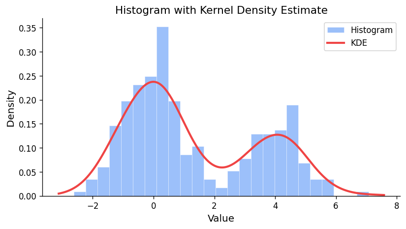
2.6 Checking the Model
Methods for assessing model fit include: (1) comparing observed and expected frequencies, (2) superimposing the fitted p.d.f. on a relative frequency histogram, (3) comparing the empirical CDF with the fitted CDF, and (4) Gaussian qqplots where the data should fall approximately on a straight line if the Gaussian model is appropriate.
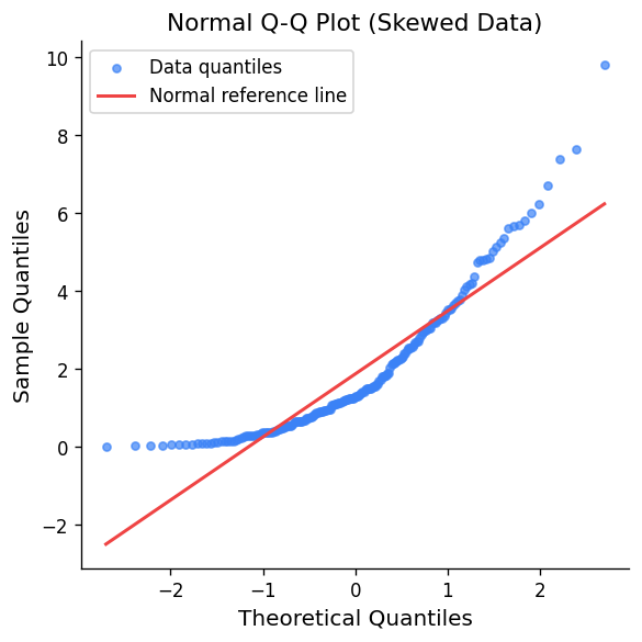
In a qqplot, U-shaped departures indicate positive skewness, S-shaped departures indicate lighter tails than the Gaussian, and points far from the line at the extremes are expected due to the rapid change of Gaussian quantiles in the tails.
Chapter 3: Planning and Conducting Empirical Studies
3.1 The PPDAC Framework
The PPDAC framework organizes empirical studies into five steps: Problem, Plan, Data, Analysis, Conclusion.
Problem
The Problem step identifies the research question. Problems are typically one of three types: descriptive (estimating attributes of a population), causative (determining causal relationships), or predictive (predicting a response variate value).
Definition 15 (Target Population). The target population or process is the collection of units to which the experimenters wish the conclusions to apply.
Definition 16 (Variate). A variate is a characteristic associated with each unit.
Definition 17 (Attribute). An attribute is a function of the variates over a population (e.g. the mean, the proportion having a certain characteristic).
Plan
Definition 18 (Study Population). The study population or study process is the collection of units available to be included in the study.
Definition 19 (Study Error). If the attributes in the study population differ from the attributes in the target population, the difference is called study error.
Definition 20 (Sampling Protocol). The sampling protocol is the procedure used to select a sample of units from the study population. The number of units sampled is the sample size.
Definition 21 (Sample Error). If the attributes in the sample differ from the attributes in the study population, the difference is called sample error.
Definition 22 (Measurement Error). If the measured value and the true value of a variate are not identical, the difference is called measurement error.
The Plan step identifies the study population, sampling protocol, variates to be measured, and measurement systems. The chain is: Target Population \(\to\) Study Population (study error) \(\to\) Sample (sample error) \(\to\) Measured variate values (measurement error).
Data, Analysis, Conclusion
The Data step collects data according to the plan, noting any deviations. The Analysis step uses numerical and graphical summaries, selects models, and performs formal inference. The Conclusion step answers the questions posed in the Problem, with discussion of potential errors and limitations.
Chapter 4: Estimation
4.1 Statistical Models and Estimation
In statistical estimation we use a model for the variability in the variate of interest and a model for how the data were collected. Unknown attributes are represented by parameters estimated using maximum likelihood and the invariance property.
4.2 Estimators and Sampling Distributions
Definition 23 (Point Estimator). A point estimator \(\tilde{\theta}\) is a random variable which is a function \(\tilde{\theta} = g(Y_1, \ldots, Y_n)\) of the random variables \(Y_1, \ldots, Y_n\). The distribution of \(\tilde{\theta}\) is called the sampling distribution of the estimator.
The sampling distribution allows us to quantify the uncertainty in a point estimate \(\hat{\theta}\). For a random sample from \(G(\mu, \sigma)\), the MLE estimator of \(\mu\) is \(\tilde{\mu} = \bar{Y} \sim G(\mu, \sigma/\sqrt{n})\), so the estimator becomes more concentrated around \(\mu\) as \(n\) increases.
4.3 Interval Estimation Using the Likelihood Function
where \(\hat{\theta}\) is the MLE. Note \(0 \le R(\theta) \le 1\).
Definition 25 (Likelihood Interval). A \(100p\%\) likelihood interval for \(\theta\) is the set \(\{\theta : R(\theta) \ge p\}\).
Guidelines for interpreting likelihood intervals: Values inside a 50% interval are very plausible; inside a 10% interval are plausible; outside a 10% interval are implausible; outside a 1% interval are very implausible.
A \(100p\%\) likelihood interval satisfies \(r(\theta) \ge \log p\).
4.4 Confidence Intervals and Pivotal Quantities
where \(p\) is called the confidence coefficient.
The confidence coefficient \(p\) means that if we drew many random samples and constructed the interval each time, then \(100p\%\) of the intervals would contain the true \(\theta\). We do NOT say \(P(\theta \in [L(y), U(y)]) = p\) for a specific observed interval.
Definition 28 (Pivotal Quantity). A pivotal quantity \(Q = Q(\mathbf{Y}, \theta)\) is a function of the data \(\mathbf{Y}\) and the unknown parameter \(\theta\) such that the distribution of \(Q\) is fully known (does not depend on \(\theta\) or any other unknown quantities).
Confidence interval construction via pivotal quantities: From \(P[a \le Q(\mathbf{Y}, \theta) \le b] = p\), rearrange to get \(P[L(\mathbf{Y}) \le \theta \le U(\mathbf{Y})] = p\).
\[\bar{y} \pm z_{(1+p)/2} \cdot \frac{\sigma}{\sqrt{n}}\]For 95%: \(\bar{y} \pm 1.96\sigma/\sqrt{n}\). For 90%: \(\bar{y} \pm 1.645\sigma/\sqrt{n}\). For 99%: \(\bar{y} \pm 2.576\sigma/\sqrt{n}\).
\[\hat{\theta} \pm 1.96\sqrt{\frac{\hat{\theta}(1-\hat{\theta})}{n}}\]Sample size for Binomial: To ensure the width of a 95% CI is at most \(2(0.03)\), choose \(n \ge (1.96/0.03)^2(0.5)^2 \approx 1068\).
4.5 The Chi-Squared and \(t\) Distributions
Chi-Squared Distribution
\[f(x;k) = \frac{1}{2^{k/2}\Gamma(k/2)} x^{(k/2)-1} e^{-x/2}, \quad x > 0\]with \(E(X) = k\) and \(\text{Var}(X) = 2k\).
Theorem 29 (Additivity of Chi-Squared). Let \(W_1, \ldots, W_n\) be independent with \(W_i \sim \chi^2(k_i)\). Then \(S = \sum_{i=1}^n W_i \sim \chi^2\!\left(\sum_{i=1}^n k_i\right)\).
Theorem 30. If \(Z \sim G(0,1)\), then \(W = Z^2 \sim \chi^2(1)\).
Corollary 31. If \(Z_1, \ldots, Z_n\) are mutually independent \(G(0,1)\) random variables, then \(S = \sum_{i=1}^n Z_i^2 \sim \chi^2(n)\).
Useful results: If \(W \sim \chi^2(1)\), then \(P(W \le w) = 2[\Phi(\sqrt{w}) - \tfrac{1}{2}]\). If \(W \sim \chi^2(2)\), then \(W \sim \text{Exponential}(2)\) and \(P(W > w) = e^{-w/2}\).
Student’s \(t\) Distribution
\[f(t;k) = c_k\left(1 + \frac{t^2}{k}\right)^{-(k+1)/2}, \quad t \in \mathbb{R}\]It is symmetric about 0, unimodal, and approaches \(G(0,1)\) as \(k \to \infty\). It has heavier tails than \(G(0,1)\) for small \(k\).
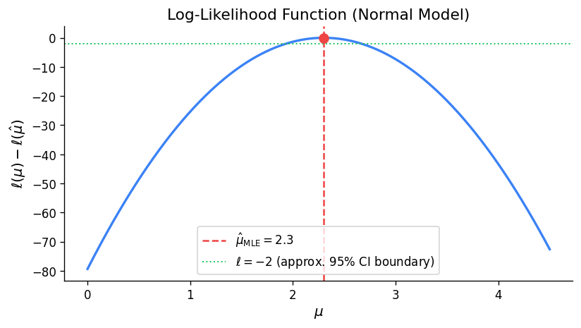
4.6 Likelihood-Based Confidence Intervals
\[\Lambda(\theta) = -2\log\frac{L(\theta)}{L(\tilde{\theta})}\]where \(\tilde{\theta}\) is the MLE.
Theorem 33 (Wilks’ Theorem). If \(L(\theta)\) is based on a random sample of size \(n\), and if \(\theta\) is the true value of the scalar parameter, then (under mild conditions) the distribution of \(\Lambda(\theta)\) converges to \(\chi^2(1)\) as \(n \to \infty\).
Theorem 34 (Likelihood Interval as Approximate CI). A \(100p\%\) likelihood interval is an approximate \(100q\%\) confidence interval where \(q = 2P(Z \ge \sqrt{-2\log p}) - 1\) and \(Z \sim N(0,1)\).
Key correspondences:
| Likelihood Interval | Approx. Confidence Level |
|---|---|
| 50% | 76% |
| 15% | 95% |
| 10% | 97% |
| 4% | 99% |
| 1% | 99.8% |
Theorem 35. If \(a\) is a value such that \(p = 2P(Z \ge a) - 1\) where \(Z \sim N(0,1)\), then the likelihood interval \(\{\theta : R(\theta) \ge e^{-a^2/2}\}\) is an approximate \(100p\%\) confidence interval.
In particular, a 15% likelihood interval is an approximate 95% confidence interval (since \(e^{-1.96^2/2} \approx 0.1465 \approx 0.15\)).
4.7 Confidence Intervals for Parameters in the \(G(\mu,\sigma)\) Model
Confidence Intervals for \(\mu\)
where \(a\) satisfies \(P(T \le a) = (1+p)/2\) with \(T \sim t(n-1)\).
Sample size for given CI width: If \(\sigma\) is approximately known, choose \(n \approx (1.96\sigma/d)^2\) where \(d\) is the desired half-width.
Confidence Intervals for \(\sigma^2\) and \(\sigma\)
where \(a\) and \(b\) satisfy \(P(U \le a) = (1-p)/2\) and \(P(U \le b) = (1+p)/2\) with \(U \sim \chi^2(n-1)\). Taking square roots gives a CI for \(\sigma\).
Chapter 5: Hypothesis Testing
5.1 Introduction
A test of hypothesis assesses whether observed data are consistent with a default (null) hypothesis \(H_0\). The logic is analogous to the legal system: \(H_0\) is assumed true unless there is strong evidence against it.
Definition 38 (Test Statistic). A test statistic or discrepancy measure \(D\) is a function of the data \(\mathbf{Y}\) constructed to measure the degree of agreement between the data and the null hypothesis \(H_0\). We define \(D\) so that \(D=0\) represents best agreement and large values indicate poor agreement.
The \(p\)-value is the probability, calculated assuming \(H_0\) is true, of observing a value of the test statistic at least as extreme as the observed value.
Guidelines for interpreting \(p\)-values:
| \(p\)-value range | Interpretation |
|---|---|
| \(> 0.10\) | No evidence against \(H_0\) |
| \(0.05 - 0.10\) | Weak evidence against \(H_0\) |
| \(0.01 - 0.05\) | Evidence against \(H_0\) |
| \(0.001 - 0.01\) | Strong evidence against \(H_0\) |
| \(\le 0.001\) | Very strong evidence against \(H_0\) |
Important remarks: (1) A small \(p\)-value is “statistically significant” evidence against \(H_0\). (2) A large \(p\)-value does NOT prove \(H_0\) is true; it means no evidence against \(H_0\). (3) The \(p\)-value is NOT the probability that \(H_0\) is true. (4) Statistical significance does not imply practical significance.
5.2 Hypothesis Testing for Parameters in the \(G(\mu,\sigma)\) Model
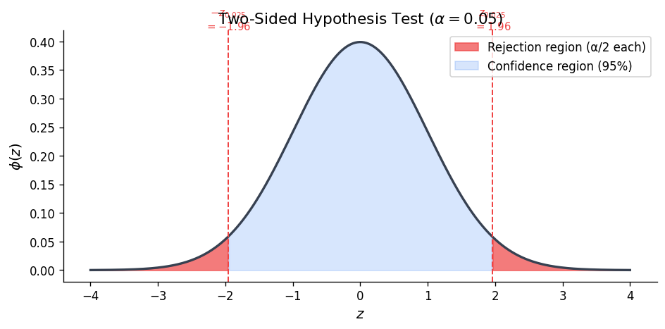
Test of \(H_0: \mu = \mu_0\) (two-sided)
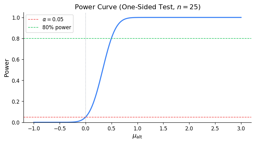
\[D = \frac{|\bar{Y} - \mu_0|}{S/\sqrt{n}}\]\[p\text{-value} = P(|T| \ge d) = 2[1 - P(T \le d)]\]One-sided test of \(H_0: \mu = \mu_0\) vs. \(\mu > \mu_0\)
Use \(D = (\bar{Y} - \mu_0)/(S/\sqrt{n})\) and \(p\text{-value} = P(T \ge d)\) where \(T \sim t(n-1)\).
Test of \(H_0: \sigma = \sigma_0\)
Use \(U = (n-1)S^2/\sigma_0^2\). Under \(H_0\), \(U \sim \chi^2(n-1)\). If \(u\) is the observed value: if \(u\) is large, \(p\text{-value} = 2P(U \ge u)\); if \(u\) is small, \(p\text{-value} = 2P(U \le u)\).
Relationship Between Testing and Confidence Intervals
The parameter value \(\theta = \theta_0\) is inside a \(100q\%\) confidence interval if and only if the \(p\)-value for testing \(H_0: \theta = \theta_0\) is greater than \(1 - q\).
5.3 Likelihood Ratio Test — One Parameter
\[\Lambda(\theta_0) = -2\log\frac{L(\theta_0)}{L(\hat{\theta})} = -2\log R(\theta_0)\]\[p\text{-value} \approx P(W \ge \lambda(\theta_0)) \text{ where } W \sim \chi^2(1)\]\[p\text{-value} \approx 2\left[1 - \Phi\!\left(\sqrt{\lambda(\theta_0)}\right)\right]\]5.4 Likelihood Ratio Test — Multiparameter
\[\Lambda = -2\log\frac{L(\hat{\boldsymbol{\theta}}_0)}{L(\hat{\boldsymbol{\theta}})} \quad \dot\sim \quad \chi^2(q) \text{ under } H_0\]where \(\hat{\boldsymbol{\theta}}_0\) is the MLE under \(H_0\) and \(\hat{\boldsymbol{\theta}}\) is the unrestricted MLE.
Chapter 6: Gaussian Response Models
6.1 Introduction
For \(n\) independently observed units: \(Y_i \sim G(\mu(\mathbf{x}_i), \sigma(\mathbf{x}_i))\) independently.
A Gaussian linear model assumes \(\mu(\mathbf{x}_i) = \beta_0 + \sum_{j=1}^k \beta_j x_{ij}\) and typically \(\sigma(\mathbf{x}_i) = \sigma\) (constant).
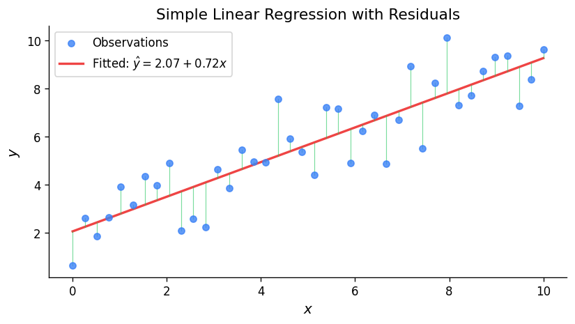
6.2 Simple Linear Regression
The model is \(Y_i \sim G(\alpha + \beta x_i, \sigma)\) independently, or equivalently \(Y_i = \alpha + \beta x_i + R_i\) where \(R_i \sim G(0, \sigma)\).
\[\hat{\beta} = \frac{S_{xy}}{S_{xx}}, \quad \hat{\alpha} = \bar{y} - \hat{\beta}\bar{x}, \quad \hat{\sigma}^2 = \frac{1}{n}\sum(y_i - \hat{\alpha} - \hat{\beta}x_i)^2 = \frac{1}{n}\left(S_{yy} - \frac{S_{xy}^2}{S_{xx}}\right)\]The unbiased estimator of \(\sigma^2\) is \(S_e^2 = \frac{1}{n-2}\sum(y_i - \hat{\alpha} - \hat{\beta}x_i)^2\).
Pivotal quantities for inference:
\[\frac{\tilde{\beta} - \beta}{S_e/\sqrt{S_{xx}}} \sim t(n-2)\]A \(100p\%\) CI for \(\beta\) is \(\hat{\beta} \pm a \cdot s_e/\sqrt{S_{xx}}\) where \(P(T \le a) = (1+p)/2\) with \(T \sim t(n-2)\).
\[\frac{\tilde{\alpha} - \alpha}{S_e\sqrt{\frac{1}{n} + \frac{\bar{x}^2}{S_{xx}}}} \sim t(n-2)\]\[\hat{\mu}(x^*) \pm a \cdot s_e\sqrt{\frac{1}{n} + \frac{(x^* - \bar{x})^2}{S_{xx}}}\]\[\hat{\mu}(x^*) \pm a \cdot s_e\sqrt{1 + \frac{1}{n} + \frac{(x^* - \bar{x})^2}{S_{xx}}}\]Model checking uses residual plots: scatterplot of standardized residuals \(\hat{r}_i = (y_i - \hat{\mu}_i)/s_e\) vs. \(x_i\) and vs. \(\hat{\mu}_i\) (should show no pattern), and a qqplot of standardized residuals (should be approximately linear).
6.3 Comparing the Means of Two Populations
Equal Variances
\[S_p^2 = \frac{\sum(Y_{1i}-\bar{Y}_1)^2 + \sum(Y_{2i}-\bar{Y}_2)^2}{n_1 + n_2 - 2}\]where \(P(T \le a) = (1+p)/2\) with \(T \sim t(n_1 + n_2 - 2)\).
Unequal Variances
\[\frac{(\bar{Y}_1 - \bar{Y}_2) - (\mu_1 - \mu_2)}{\sqrt{S_1^2/n_1 + S_2^2/n_2}}\]\[\bar{y}_1 - \bar{y}_2 \pm 1.96\sqrt{\frac{s_1^2}{n_1} + \frac{s_2^2}{n_2}}\]Paired Data
\[\frac{\bar{D} - \mu_D}{S_D/\sqrt{n}} \sim t(n-1)\]6.4 General Gaussian Response Models
For the general model \(Y_i \sim G(\mu_i, \sigma)\) with \(\mu_i = \sum_{j=1}^k \beta_j x_{ij}\), written in matrix form as \(\boldsymbol{\mu} = X\boldsymbol{\beta}\):
Theorem 43 (Properties of MLEs).
- Each \(\tilde{\beta}_j\) is Normally distributed with \(E(\tilde{\beta}_j) = \beta_j\) and variance equal to the \(j\)th diagonal element of \(\sigma^2(X^TX)^{-1}\).
- The random variable \(W = n\tilde{\sigma}^2/\sigma^2 = (n-k)S_e^2/\sigma^2 \sim \chi^2(n-k)\).
- \(W\) is independent of \((\tilde{\beta}_1, \ldots, \tilde{\beta}_k)\).
where \(c_j\) is the \(j\)th diagonal element of \((X^TX)^{-1}\). A \(100p\%\) CI for \(\beta_j\) takes the form \(\hat{\beta}_j \pm a \cdot s_e\sqrt{c_j}\).
Chapter 7: Multinomial Models and Goodness of Fit Tests
7.1 Likelihood Ratio Test for the Multinomial Model
\[\Lambda = 2\sum_{j=1}^k y_j \log\frac{y_j}{e_j}\]where \(e_j = n\theta_j(\hat{\boldsymbol{\phi}})\) are the expected frequencies under \(H_0\). Under \(H_0\) with large \(n\), \(\Lambda \dot\sim \chi^2(k - 1 - p)\).
\[D = \sum_{j=1}^k \frac{(y_j - e_j)^2}{e_j}\]which also has approximately a \(\chi^2(k-1-p)\) distribution under \(H_0\). All expected frequencies should be at least 5 for the approximation to be adequate.
7.2 Goodness of Fit Tests
A goodness of fit test assesses whether a proposed probability model is consistent with the data. The procedure is:
- Compute the MLE \(\hat{\boldsymbol{\phi}}\) of any unknown parameters under \(H_0\).
- Calculate expected frequencies \(e_j\). Combine categories if any \(e_j < 5\).
- Compute \(\Lambda\) or \(D\).
- Compute \(p\text{-value} \approx P(W \ge \lambda)\) where \(W \sim \chi^2(k-1-p)\).
For continuous distributions, partition the range into intervals and count observations in each interval to form a Multinomial model. Choose 4–10 intervals with all expected frequencies at least 5.
7.3 Two-Way (Contingency) Tables
\[H_0: \theta_{ij} = \theta_{i\cdot}\theta_{\cdot j} \quad \text{for all } i, j\]\[(ab - 1) - p = (a-1)(b-1)\]\[\Lambda = 2\sum_{i=1}^a \sum_{j=1}^b y_{ij}\log\frac{y_{ij}}{e_{ij}} \quad \dot\sim \quad \chi^2((a-1)(b-1))\]Chapter 8: Causal Relationships
8.1 Establishing Causation
Establishing a causal relationship between two variates is much more difficult than establishing an association. The three types of empirical studies differ in their ability to support causal claims:
- Experimental studies provide the strongest evidence for causation because the experimenter controls the explanatory variate and can use randomization to balance other factors.
- Observational studies can reveal associations but confounding variables (lurking variables related to both the explanatory and response variates) make it difficult to establish causation.
- Sample surveys describe populations but generally cannot establish causation.
8.2 Experimental Studies
In a properly designed experiment: (1) the experimenter manipulates the explanatory variate, (2) subjects are randomly assigned to treatment groups (randomization balances confounders), (3) ideally the study is double-blind (neither subjects nor evaluators know treatment assignments), and (4) a control group (placebo) is used for comparison. Randomization is the key feature that distinguishes experiments from observational studies and allows causal conclusions.
8.3 Observational Studies
In observational studies, the researcher does not control the explanatory variate. Confounding occurs when an extraneous variable is associated with both the explanatory and response variates. Even with sophisticated statistical adjustments, observational studies can only establish associations, not causation. Criteria for assessing potential causal relationships from observational data include: strength of association, consistency across studies, temporal ordering (cause precedes effect), dose-response relationship, and biological plausibility.
8.4 Simpson’s Paradox
An association between two variates that holds in a combined population can reverse direction when the population is divided into subgroups. This phenomenon, known as Simpson’s paradox, arises from confounding and demonstrates the danger of drawing causal conclusions from observational data without accounting for lurking variables.