PMATH 351: Real Analysis

Stephen New

Estimated study time: 5 hr 56 min

Table of contents

These notes synthesize material from multiple sources: Stephen New’s Fall 2018 lecture notes (primary), Kenneth Davidson’s PMATH 351 instructor notes, Brian Forrest’s PMATH 351 instructor notes, Laurent Marcoux’s PMATH 351 instructor notes, and student notes by Felix Zhou (Fall 2019, Davidson’s section), Richard Wu (Fall 2018, Forrest’s section), and David Duan. All sources are credited below.

Chapter 1: Cardinality

The first chapter lays the foundational set-theoretic framework upon which the rest of real analysis is built. Before we can discuss metric spaces and topology, we need a precise understanding of the “size” of sets — finite, countable, and uncountable. These distinctions will later be essential for understanding separability, the structure of the real line, and the Baire Category Theorem.

1.1 Functions, Injections, and Surjections

We begin by recalling the basic vocabulary of functions, which will be used throughout the course.

Definition 1.1 (Image and Preimage). Let \(X\) and \(Y\) be sets and let \(f : X \to Y\). The domain of \(f\) is \(X\) and the range of \(f\) is \(f(X) = \{f(x) \mid x \in X\}\). For \(A \subseteq X\), the image of \(A\) under \(f\) is \(f(A) = \{f(x) \mid x \in A\}\). For \(B \subseteq Y\), the inverse image (or preimage) of \(B\) under \(f\) is \(f^{-1}(B) = \{x \in X \mid f(x) \in B\}\).

Proposition 1.2 (Set-theoretic properties of images and preimages). Let \(f: X \to Y\).

\(f^{-1}(B_1 \cup B_2) = f^{-1}(B_1) \cup f^{-1}(B_2)\) and \(f^{-1}(B_1 \cap B_2) = f^{-1}(B_1) \cap f^{-1}(B_2)\).
\(f^{-1}(B^c) = (f^{-1}(B))^c\).
\(f(A_1 \cup A_2) = f(A_1) \cup f(A_2)\), but in general \(f(A_1 \cap A_2) \subseteq f(A_1) \cap f(A_2)\) with equality when \(f\) is injective.
\(A \subseteq f^{-1}(f(A))\) with equality when \(f\) is injective; \(f(f^{-1}(B)) \subseteq B\) with equality when \(f\) is surjective.

These properties are fundamental: property (1) and (2) mean that preimages commute perfectly with all set operations. This is precisely why the topological characterization of continuity (preimages of open sets are open) is so natural.

Definition 1.3 (Injective, Surjective, Bijective). Let \(f : X \to Y\).

\(f\) is injective (one-to-one) if for all \(x_1, x_2 \in X\), \(f(x_1) = f(x_2)\) implies \(x_1 = x_2\).
\(f\) is surjective (onto) if \(f(X) = Y\), i.e., every element of \(Y\) is hit.
\(f\) is bijective (invertible) if it is both injective and surjective.

When \(f\) is bijective, we define its inverse \(f^{-1}: Y \to X\) by letting \(f^{-1}(y)\) be the unique \(x \in X\) with \(f(x) = y\). The fundamental algebraic fact about composition is that it preserves injectivity and surjectivity.

Theorem 1.4 (Composition preserves injectivity/surjectivity). Let \(f: X \to Y\) and \(g: Y \to Z\).

If \(f\) and \(g\) are both injective, then \(g \circ f\) is injective.
If \(f\) and \(g\) are both surjective, then \(g \circ f\) is surjective.
If \(f\) and \(g\) are both bijective, then \(g \circ f\) is bijective with \((g \circ f)^{-1} = f^{-1} \circ g^{-1}\).

The relationship between injectivity/surjectivity and the existence of one-sided inverses is fundamental to both algebra and analysis:

Theorem 1.5 (Left and right inverses). Let \(X, Y\) be nonempty sets and \(f: X \to Y\).

\(f\) is injective if and only if \(f\) has a left inverse (a function \(g: Y \to X\) with \(g \circ f = I_X\)).
\(f\) is surjective if and only if \(f\) has a right inverse (a function \(h: Y \to X\) with \(f \circ h = I_Y\)).
\(f\) is bijective if and only if \(f\) has both a left inverse \(g\) and a right inverse \(h\), in which case \(g = h = f^{-1}\).

Note that the proof that every surjection has a right inverse requires the Axiom of Choice — we must simultaneously choose, for each \(y \in Y\), a preimage \(x_y \in X\).

Corollary 1.6. There exists an injection \(f: X \to Y\) if and only if there exists a surjection \(g: Y \to X\).

1.2 Cardinality and Ordering

With injections and bijections in hand, we can now compare the “sizes” of sets.

Definition 1.7 (Cardinality). Let \(A\) and \(B\) be sets.

We write \(|A| = |B|\) when there exists a bijection \(f: A \to B\).
We write \(|A| \le |B|\) when there exists an injection \(f: A \to B\).
We write \(|A| < |B|\) when \(|A| \le |B|\) and \(|A| \ne |B|\).

The relation \(|A| = |B|\) is an equivalence relation: it is reflexive (via the identity), symmetric (via the inverse), and transitive (via composition). The relation \(|A| \le |B|\) is reflexive and transitive — but showing it is antisymmetric requires a deep theorem.

Example 1.8. The map \(f: \mathbb{N} \to 2\mathbb{N}\) given by \(f(k) = 2k\) is a bijection, so \(|\mathbb{N}| = |2\mathbb{N}|\). The map \(g: \mathbb{N} \to \mathbb{Z}\) given by \(g(2k) = k\), \(g(2k+1) = -k-1\) is a bijection, so \(|\mathbb{Z}| = |\mathbb{N}|\). The map \(h: \mathbb{N} \times \mathbb{N} \to \mathbb{N}\) given by \(h(k,l) = 2^k(2l+1) - 1\) is a bijection, so \(|\mathbb{N} \times \mathbb{N}| = |\mathbb{N}|\).

Definition 1.9 (Finite, Countable, Uncountable). Let \(S_n = \{0, 1, \ldots, n-1\}\). A set \(A\) is finite if \(|A| = |S_n|\) for some \(n \in \mathbb{N}\). A set is countable (or countably infinite) if \(|A| = |\mathbb{N}|\). A set is at most countable if it is finite or countable. A set is uncountable if it is neither finite nor countable.

A crucial characterization of infinite sets connects injectivity and surjectivity:

Theorem 1.10 (Characterizations of infinite sets). For a set \(A\), the following are equivalent:

\(A\) is infinite.
\(A\) contains a countable subset.
\(|\mathbb{N}| \le |A|\).
There exists a map \(f: A \to A\) which is injective but not surjective.

The implication (4) \(\Rightarrow\) (1) is proved by its contrapositive: every injective map from a finite set to itself is surjective (the pigeonhole principle, proved by induction on \(|A|\)).

1.3 The Cantor–Schroeder–Bernstein Theorem

The antisymmetry of cardinality comparison is far from obvious. It is resolved by the following landmark result.

Theorem 1.11 (Cantor--Schroeder--Bernstein). If \(|A| \le |B|\) and \(|B| \le |A|\), then \(|A| = |B|\).

Proof (Sketch). Choose injections \(f: A \to B\) and \(g: B \to A\). Let \(X = f(g(B))\), \(Y = f(A)\), and \(Z = B\), so \(X \subseteq Y \subseteq Z\) with \(|X| = |Z|\). The composite \(h = f \circ g: Z \to X\) is a bijection. Define sets \(Z_n, Y_n\) recursively by \(Z_0 = Z\), \(Y_0 = Y\), \(Z_n = h(Z_{n-1})\), \(Y_n = h(Y_{n-1})\). Then \(Z_0 \supseteq Y_0 \supseteq Z_1 \supseteq Y_1 \supseteq \cdots\). Let \(U_n = Z_n \setminus Y_n\), \(U = \bigcup_{n=0}^{\infty} U_n\), and \(V = Z \setminus U\). Define \(H: Z \to Y\) by \(H(x) = h(x)\) if \(x \in U\) and \(H(x) = x\) if \(x \in V\). One verifies that \(H\) is a bijection.

This theorem is remarkable because it does not require the Axiom of Choice — the proof is entirely constructive. It allows us to establish equalities of cardinality by exhibiting injections in both directions, which is often much easier than constructing an explicit bijection.

1.4 Countable and Uncountable Sets

Theorem 1.12 (Closure properties of countable sets).

If \(A\) and \(B\) are countable, then so is \(A \times B\).
If \(A\) and \(B\) are countable, then so is \(A \cup B\).
A countable union of countable sets is countable.
\(\mathbb{Q}\) is countable.

Part (4) follows because the map \(g: \mathbb{Q} \to \mathbb{Z} \times \mathbb{Z}\) sending each fraction in lowest terms \(\frac{a}{b}\) to the pair \((a,b)\) is injective, and \(\mathbb{Z} \times \mathbb{Z}\) is countable.

Now for the other direction — uncountability. Cantor’s argument is one of the most beautiful in all of mathematics.

Theorem 1.13 (Cantor's Theorem). For every set \(A\), \(|A| < |\mathcal{P}(A)|\).

Proof. The map \(a \mapsto \{a\}\) is an injection from \(A\) to \(\mathcal{P}(A)\), so \(|A| \le |\mathcal{P}(A)|\). Suppose for contradiction that \(g: A \to \mathcal{P}(A)\) is surjective. Let \(S = \{a \in A \mid a \notin g(a)\}\). Then \(S\) cannot be in the range of \(g\): if \(g(a) = S\), then \(a \in S \iff a \notin g(a) \iff a \notin S\), a contradiction. So no surjection exists, hence \(|A| \ne |\mathcal{P}(A)|\).

Remark (Russell's Paradox). The diagonal argument in Cantor's theorem is closely related to Russell's Paradox. If we naively allowed a "set of all sets" \(\mathcal{U}\), the identity map \(\mathrm{id}: \mathcal{U} \to \mathcal{P}(\mathcal{U})\) would be a surjection, contradicting Cantor's theorem. This is why modern set theory (ZFC) restricts set formation through axioms — in particular, the Axiom Schema of Separation, which only allows forming subsets of existing sets.

Corollary 1.14. \(\mathbb{R}\) is uncountable.

Proof. One shows that \(|2^{\mathbb{N}}| \le |\mathbb{R}|\) using decimal expansions. Since \(|\mathbb{N}| < |2^{\mathbb{N}}| \le |\mathbb{R}|\), we have \(|\mathbb{N}| < |\mathbb{R}|\), so \(\mathbb{R}\) is uncountable.

In fact, one can show that \(|\mathbb{R}| = |2^{\mathbb{N}}| = |\mathcal{P}(\mathbb{N})|\) using the Cantor–Schroeder–Bernstein theorem. We write \(|\mathbb{R}| = \mathfrak{c}\) (the cardinality of the continuum) and \(|\mathbb{N}| = \aleph_0\). Cantor’s theorem yields an infinite hierarchy of infinite cardinalities: \(\aleph_0 < 2^{\aleph_0} < 2^{2^{\aleph_0}} < \cdots\). There is no “largest” cardinal number.

Theorem 1.15 (Cantor's Diagonal Argument). The set \(2^{\mathbb{N}}\) of all binary sequences is uncountable.

Proof. Suppose \(f: \mathbb{N} \to 2^{\mathbb{N}}\) is a surjection, with \(f(n) = (a_{n,1}, a_{n,2}, \ldots)\). Define a sequence \(b = (b_1, b_2, \ldots)\) by \(b_n = 1 - a_{n,n}\). Then \(b\) differs from \(f(n)\) in the \(n\)-th coordinate for every \(n\), so \(b \notin \operatorname{range}(f)\) — a contradiction.

Alternative proof that \(\mathbb{R}\) is uncountable (decimal argument). Suppose \(\mathbb{R}\) is countable, and list all real numbers in \([0,1)\) as \(r_1, r_2, r_3, \ldots\), where each \(r_n\) has a decimal expansion \(r_n = 0.d_{n,1}\, d_{n,2}\, d_{n,3}\, \cdots\). Construct a new real number \(s = 0.s_1\, s_2\, s_3\, \cdots\) by choosing \(s_n\) to differ from \(d_{n,n}\) (for definiteness, let \(s_n = 3\) if \(d_{n,n} \ne 3\), and \(s_n = 7\) if \(d_{n,n} = 3\) --- this avoids the issue of non-unique decimal representations like \(0.999\ldots = 1.000\ldots\)). Then \(s \ne r_n\) for all \(n\), since \(s\) and \(r_n\) differ in the \(n\)-th decimal place, and neither has an ambiguous decimal expansion. This contradicts surjectivity, so \([0,1)\) (hence \(\mathbb{R}\)) is uncountable.

Remark (Cardinality hierarchy of common sets). In summary, the set-theoretic landscape is: \[ |\emptyset| = 0 < |S_n| = n < |\mathbb{N}| = |\mathbb{Z}| = |\mathbb{Q}| = \aleph_0 < |\mathbb{R}| = |C| = |[0,1]| = |\mathcal{P}(\mathbb{N})| = 2^{\aleph_0} = \mathfrak{c}, \]

where \(C\) is the Cantor set. The algebraic numbers form a countable set (there are only countably many integer polynomials, each with finitely many roots), so the transcendental numbers are uncountable — indeed, they have cardinality \(\mathfrak{c}\). This is remarkable: transcendental numbers are “almost all” reals, yet explicitly constructing them (like \(e\) and \(\pi\)) requires significant effort.

1.5 The Axiom of Choice and Zorn’s Lemma

Several key results in this course (existence of right inverses for surjections, comparability of cardinals, bases for vector spaces) require the Axiom of Choice or one of its equivalents.

Axiom of Choice (AC). Given any collection \(\{A_\alpha\}_{\alpha \in I}\) of nonempty sets, there exists a choice function \(f: I \to \bigcup_{\alpha \in I} A_\alpha\) such that \(f(\alpha) \in A_\alpha\) for every \(\alpha \in I\).

The Axiom of Choice is intuitively obvious for finite collections and even for countable collections (where one can make choices sequentially), but it is an independent axiom for uncountable collections. It was shown to be consistent with ZF by Gödel (1938) and independent of ZF by Cohen (1963).

Zorn's Lemma. Let \((P, \le)\) be a nonempty partially ordered set in which every chain (totally ordered subset) has an upper bound. Then \(P\) has a maximal element.

Well-Ordering Principle. Every set can be well-ordered, i.e., given a total order in which every nonempty subset has a least element.

Remark. The Axiom of Choice, Zorn's Lemma, and the Well-Ordering Principle are all equivalent in ZF set theory. Zorn's Lemma is the version most commonly used in analysis and algebra. It is applied, for example, to prove that every vector space has a basis, and that any two cardinalities are comparable: for any sets \(A\) and \(B\), either \(|A| \le |B|\) or \(|B| \le |A|\).

Example 1.14a (Consequences of the Axiom of Choice in analysis). The Axiom of Choice has several surprising consequences in real analysis:

Non-measurable sets: The Vitali construction uses AC to produce a subset of \([0,1]\) that is not Lebesgue measurable. Partition \([0,1)\) by the equivalence relation \(x \sim y\) iff \(x - y \in \mathbb{Q}\). Use AC to choose one representative from each equivalence class, forming a set \(V\). If \(V\) were measurable, then \([0,1) = \bigcup_{q \in \mathbb{Q} \cap [0,1)} (V + q \mod 1)\) would give \(1 = \sum m(V)\), which is impossible since either \(m(V) = 0\) (giving sum 0) or \(m(V) > 0\) (giving sum \(\infty\)).
Banach--Tarski paradox: AC implies that a solid ball in \(\mathbb{R}^3\) can be decomposed into finitely many pieces and reassembled (via rotations and translations) into two solid balls of the same size. The pieces are necessarily non-measurable.
Hamel bases: AC guarantees that \(\mathbb{R}\) has a basis as a \(\mathbb{Q}\)-vector space, although no explicit Hamel basis can be constructed. The existence of a Hamel basis implies the existence of discontinuous additive functions \(f: \mathbb{R} \to \mathbb{R}\) satisfying \(f(x+y) = f(x) + f(y)\) --- the graph of such a function is dense in \(\mathbb{R}^2\).

These pathologies illustrate why the relationship between AC and analysis is subtle: AC is essential for many positive results (the Hahn--Banach theorem, Tychonoff's theorem, the existence of maximal ideals) but also produces "paradoxical" objects.

1.5a Well-Ordered Sets, Transfinite Induction, and Ordinal Numbers

The Axiom of Choice is most naturally understood through the lens of well-ordered sets — posets in which every nonempty subset has a minimum element. The ordinary induction principle on \(\mathbb{N}\) generalizes to any well-ordered set, and the resulting framework of transfinite induction is one of the most powerful tools in set theory and logic.

Definition 1.14b (Well-Ordered Set). A nonempty partially ordered set \((X, \le)\) is well-ordered if every nonempty subset \(A \subseteq X\) has a minimum element — an element \(m \in A\) such that \(m \le a\) for all \(a \in A\).

Every well-ordered set is automatically totally ordered: given \(x, y \in X\), the subset \(\{x, y\}\) has a minimum element, which must be \(\le\) the other. The natural numbers \(\mathbb{N}\) under the usual order are the archetypal well-ordered set; the reals \(\mathbb{R}\) are not well-ordered (the open interval \((0,1)\) has no minimum element).

A slightly exotic example illuminates the concept: let \(\omega + 7 = \{1, 2, 3, \ldots\} \cup \{\omega, \omega+1, \omega+2, \ldots, \omega+6\}\), with the ordering \(n \le \omega + k\) for all \(n \in \mathbb{N}\) and \(0 \le k \le 6\), and \(\omega + i \le \omega + j\) when \(i \le j\). This set is well-ordered: it looks like the natural numbers followed by seven extra elements “after infinity.” The element \(\omega\) has no immediate predecessor — no largest natural number precedes it — yet every nonempty subset still has a minimum.

Theorem 1.14c (Principle of Transfinite Induction). Let \((X, \le)\) be a well-ordered set and \(S \subseteq X\). Suppose that for every \(x \in X\), \[ \{y \in X : y < x\} \subseteq S \implies x \in S. \]

Then \(S = X\).

Proof. If \(S \ne X\), let \(x_0 = \min(X \setminus S)\), which exists since \(X \setminus S\) is nonempty and \(X\) is well-ordered. By definition of \(x_0\), every \(y < x_0\) belongs to \(S\), i.e., \(\{y : y < x_0\} \subseteq S\). By hypothesis, \(x_0 \in S\), a contradiction. Hence \(S = X\). \(\square\)

This generalizes ordinary induction: when \(X = \mathbb{N}\), the condition \(\{y < n\} \subseteq S \Rightarrow n \in S\) is exactly “if \(S(0), S(1), \ldots, S(n-1)\) hold then \(S(n)\) holds,” which is strong induction. When \(X\) contains limit ordinals (elements with no immediate predecessor, like \(\omega\)), transfinite induction handles them naturally via the hypothesis: if \(S\) contains all elements before a limit ordinal \(\lambda\), then \(S\) contains \(\lambda\) too.

Culture: Ordinal Numbers. The notion of well-ordered sets leads naturally to the concept of ordinal numbers, which measure the “order type” of well-ordered sets in the same way that cardinal numbers measure their size.

Two well-ordered sets \((A, \le_A)\) and \((B, \le_B)\) are called order-isomorphic if there exists an order-preserving bijection \(f: A \to B\) (i.e., \(a_1 \le_A a_2 \Rightarrow f(a_1) \le_B f(a_2)\)). An ordinal number is an equivalence class of well-ordered sets under order isomorphism.

The finite ordinals are just the natural numbers: \(0 = \emptyset\), \(1 = \{0\}\), \(2 = \{0,1\}\), and so on, with \(n = \{0, 1, \ldots, n-1\}\) for each \(n \in \mathbb{N}\). The first infinite ordinal is \(\omega = \{0, 1, 2, \ldots\}\), the order type of \(\mathbb{N}\). Beyond \(\omega\) lie \(\omega + 1, \omega + 2, \ldots\), then \(\omega + \omega = \omega \cdot 2\), then \(\omega^2, \omega^3, \ldots, \omega^\omega\), and so on through a transfinite hierarchy.

One striking feature is that ordinal addition is not commutative. If we prepend a single element to \(\mathbb{N}\), we get a set order-isomorphic to \(\mathbb{N}\) itself (just shift all indices), so \(1 + \omega = \omega\). But \(\omega + 1\) consists of \(\mathbb{N}\) followed by one extra element after all natural numbers; this has a maximum element while \(\omega\) does not, so \(\omega + 1 \ne \omega\). Thus \(1 + \omega = \omega \ne \omega + 1\).

This non-commutativity contrasts with cardinal arithmetic, where infinite cardinals satisfy \(\kappa + \lambda = \lambda + \kappa = \max(\kappa, \lambda)\). The distinction reflects the fact that ordinals care about order, while cardinals care only about size.

1.5b Proof of the Equivalences: AC, Zorn’s Lemma, and the Well-Ordering Principle

The three statements AC, ZL, and WO stated in §1.5 are equivalent in Zermelo–Fraenkel set theory. We give the complete proof here, following Marcoux’s treatment. The argument is the most technical in Chapter 1, but it pays off: it shows how all three principles are facets of the same underlying idea — that “arbitrary choices can always be made simultaneously.”

Definition 1.14d (Initial Segment). Let \((X, \le)\) be a poset, \(C \subseteq X\) a chain, and \(d \in C\). The initial segment of \(C\) at \(d\) is \[ P(C, d) = \{c \in C : c < d\}. \]

Examples. For \((R, \le)\), the interval \((-\infty, r)\) is an initial segment. For \(\mathbb{N}\), the set \(\{1, 2, \ldots, n\}\) is the initial segment at \(n+1\).

Theorem 1.14e. The following are equivalent:

(AC) For any nonempty collection \(\{X_\lambda\}_{\lambda \in \Lambda}\) of nonempty sets, \(\prod_{\lambda \in \Lambda} X_\lambda \ne \emptyset\).
(ZL) Let \((Y, \le)\) be a nonempty poset in which every chain has an upper bound. Then \(Y\) has a maximal element.
(WO) Every nonempty set \(Z\) admits a well-ordering.

Proof.

(AC \(\Rightarrow\) ZL). Suppose every chain in \((X, \le)\) has an upper bound, but assume for contradiction that \(X\) has no maximal element. Then every chain \(C\) has a strict upper bound — an element strictly greater than every upper bound. By AC, we can choose one strict upper bound \(f(C)\) for each chain \(C\); if \(C = \emptyset\), choose any \(x_0 \in X\) and set \(f(\emptyset) = x_0\).

Call a subset \(A \subseteq X\) a \(P\)-set if (I) \((A, \le)\) is well-ordered, and (II) for every \(x \in A\), \(x = f(P(A, x))\) — each element of \(A\) is the chosen strict upper bound of its initial segment within \(A\).

Claim 1: If \(A\) and \(B\) are both \(P\)-sets and \(A \ne B\), then one is an initial segment of the other. (The proof compares minimum elements of \(A \setminus B\) and \(B \setminus A\), using the well-orderings and property (II) to establish the equality \(P(A,x) = P(B,y)\) at the key element, and concludes that one is an initial segment of the other.)

Let \(V = \bigcup\{A \subseteq X : A \text{ is a } P\text{-set}\}\).

Claim 2: \(V\) is itself a \(P\)-set. (Follows from Claim 1: the union of a “compatible” family of well-ordered sets is well-ordered, and the property (II) is inherited by the union.)

Now set \(w = f(V)\). Then \(V \cup \{w\}\) is a \(P\)-set strictly containing \(V\), so \(w \in V\), contradicting \(w = f(V)\) being a strict upper bound for \(V\). This contradiction shows that \(X\) must have had a maximal element.

(ZL \(\Rightarrow\) WO). Let \(X \ne \emptyset\). Let \(\mathcal{A}\) be the collection of pairs \((Y, \le_Y)\) where \(Y \subseteq X\) and \(\le_Y\) is a well-ordering of \(Y\). Partially order \(\mathcal{A}\) by: \((A, \le_A) \le (B, \le_B)\) if \(A\) is an initial segment of \(B\). Any chain in \(\mathcal{A}\) has an upper bound (the union with the induced ordering). By ZL, \(\mathcal{A}\) has a maximal element \((M, \le_M)\). If \(M \ne X\), pick \(x_0 \in X \setminus M\) and extend \(\le_M\) to a well-ordering of \(M \cup \{x_0\}\) by declaring \(x_0\) greater than everything in \(M\); this contradicts maximality of \((M, \le_M)\). Hence \(M = X\), giving a well-ordering of \(X\).

(WO \(\Rightarrow\) AC). Let \(\{X_\lambda\}_{\lambda \in \Lambda}\) be a nonempty collection of nonempty sets. By WO, each \(X_\lambda\) can be well-ordered, so it has a minimum element \(\min X_\lambda\). Define the choice function \(f(\lambda) = \min X_\lambda\). \(\square\)

The implication AC \(\Rightarrow\) ZL deserves a comment: the detailed verification of Claims 1 and 2 is intricate (it occupies several pages in Marcoux’s notes), but the core idea is clean — a maximal “coherent” well-ordered structure built by iterating the choice function must equal all of \(X\), and that yields a contradiction unless a maximal element exists.

1.6 Cardinal Arithmetic

Using the Cantor–Schroeder–Bernstein Theorem (Theorem 1.11) and the closure properties of countable sets (Theorem 1.12), we can develop a full arithmetic of cardinal numbers, extending ordinary arithmetic to infinite quantities.

Definition 1.16 (Cardinal Arithmetic). For cardinals \(\kappa\) and \(\lambda\), define: \[ \kappa + \lambda = |(\kappa \times \{0\}) \cup (\lambda \times \{1\})|, \quad \kappa \cdot \lambda = |\kappa \times \lambda|, \quad \kappa^\lambda = |\kappa^\lambda| \text{ (the set of functions } \lambda \to \kappa\text{)}. \]

The key laws include commutativity and associativity of addition and multiplication, distributivity, and the exponential laws:

\[ \kappa^{\lambda + \mu} = \kappa^\lambda \cdot \kappa^\mu, \quad (\kappa^\lambda)^\mu = \kappa^{\lambda \cdot \mu}, \quad (\kappa \cdot \lambda)^\mu = \kappa^\mu \cdot \lambda^\mu. \]

For infinite cardinals, the arithmetic simplifies dramatically: if \(\kappa\) is an infinite cardinal, then \(\kappa + \kappa = \kappa \cdot \kappa = \kappa\). Also, \(2^{\aleph_0} = \mathfrak{c}\) and \(\mathfrak{c}^{\aleph_0} = \mathfrak{c}\). The Continuum Hypothesis posits that there is no cardinal strictly between \(\aleph_0\) and \(\mathfrak{c}\); this is independent of ZFC (proved by Gödel and Cohen).

Example 1.17 (Important cardinality computations).

\(|\mathbb{R}| = |2^{\mathbb{N}}| = |\mathcal{P}(\mathbb{N})| = \mathfrak{c}\).
\(|\mathbb{R}^n| = \mathfrak{c}\) for every \(n \ge 1\), and \(|\mathbb{R}^{\mathbb{N}}| = \mathfrak{c}\).
The set of all continuous functions \(f: \mathbb{R} \to \mathbb{R}\) has cardinality \(\mathfrak{c}\), since a continuous function is determined by its values on \(\mathbb{Q}\).
The set of all functions \(f: \mathbb{R} \to \mathbb{R}\) has cardinality \(2^{\mathfrak{c}} > \mathfrak{c}\).

Remark (Cardinality constraints in analysis). These computations have important consequences for analysis:

Since \(|C(\mathbb{R}, \mathbb{R})| = \mathfrak{c}\) but \(|\mathbb{R}^{\mathbb{R}}| = 2^{\mathfrak{c}} > \mathfrak{c}\), "most" functions \(\mathbb{R} \to \mathbb{R}\) are discontinuous everywhere. The continuous functions form a negligible minority from the cardinality standpoint.
The set of Borel sets in \(\mathbb{R}\) has cardinality \(\mathfrak{c}\) (a consequence of the transfinite construction of the Borel \(\sigma\)-algebra), while the set of Lebesgue measurable sets has cardinality \(2^{\mathfrak{c}}\). Thus "most" Lebesgue measurable sets are not Borel sets.
Every separable metric space has cardinality at most \(\mathfrak{c}\). Since the spaces \(C[0,1]\), \(\ell^p\) (for \(p < \infty\)), and \(\mathbb{R}^n\) are all separable and have cardinality exactly \(\mathfrak{c}\), they are "as large as possible" for separable spaces.

These observations illustrate how the set-theoretic tools of Chapter 1 inform the analytical developments of subsequent chapters.

Chapter 2: Metric Spaces

Having established the set-theoretic foundations in Chapter 1, we now introduce the central object of study in this course: the metric space. A metric space is a set equipped with a distance function that generalizes the familiar notion of distance in \(\mathbb{R}^n\). This abstraction allows us to develop a unified theory of convergence, continuity, and completeness that applies far beyond Euclidean space.

2.1 Inner Product Spaces and Normed Vector Spaces

The most natural and important source of metric spaces is normed vector spaces, which themselves often arise from inner product spaces. We begin with these algebraic structures before abstracting to the purely topological setting.

Definition 2.1 (Inner Product). Let \(U\) be a vector space over \(\mathbb{F} \in \{\mathbb{R}, \mathbb{C}\}\). An inner product on \(U\) is a function \(\langle \cdot, \cdot \rangle: U \times U \to \mathbb{F}\) such that for all \(u, v, w \in U\) and \(t \in \mathbb{F}\):

Sesquilinearity: \(\langle u + v, w\rangle = \langle u, w\rangle + \langle v, w\rangle\), \(\langle tu, v\rangle = t\langle u, v\rangle\), and \(\langle u, tv\rangle = \bar{t}\langle u, v\rangle\).
Conjugate symmetry: \(\langle u, v\rangle = \overline{\langle v, u\rangle}\).
Positive definiteness: \(\langle u, u\rangle \ge 0\) with equality iff \(u = 0\).

Definition 2.2 (Norm). Let \(V\) be a vector space over \(\mathbb{F} \in \{\mathbb{R}, \mathbb{C}\}\). A norm on \(V\) is a function \(\|\cdot\|: V \to [0, \infty)\) satisfying:

Positive definiteness: \(\|v\| = 0 \iff v = 0\).
Positive homogeneity: \(\|\lambda v\| = |\lambda| \|v\|\) for all \(\lambda \in \mathbb{F}\), \(v \in V\).
Triangle inequality: \(\|u + v\| \le \|u\| + \|v\|\) for all \(u, v \in V\).

The pair \((V, \|\cdot\|)\) is a normed vector space (or normed linear space). A seminorm satisfies (2) and (3) and \(\|0\| = 0\), but may have nonzero vectors of zero norm.

Every inner product space is a normed vector space via \(\|x\| = \langle x, x\rangle^{1/2}\). The triangle inequality follows from the Cauchy–Schwarz inequality.

Theorem 2.3 (Cauchy--Schwarz Inequality). Let \(U\) be an inner product space. For all \(u, v \in U\): \[ |\langle u, v\rangle| \le \|u\| \|v\|, \]

with equality if and only if \(\{u, v\}\) is linearly dependent.

Proof. If \(\{u, v\}\) is linearly dependent, say \(v = tu\), then \(|\langle u, v\rangle| = |t| \|u\|^2 = \|u\| \|tu\| = \|u\| \|v\|\). Now suppose \(\{u, v\}\) is linearly independent. Then \(v - \frac{\langle v, u\rangle}{\|u\|^2} u \ne 0\), so \[ 0 < \left\|v - \frac{\langle v, u\rangle}{\|u\|^2} u\right\|^2 = \|v\|^2 - \frac{|\langle u, v\rangle|^2}{\|u\|^2}, \]

giving \(|\langle u, v\rangle|^2 < \|u\|^2 \|v\|^2\).

The Cauchy–Schwarz inequality yields the triangle inequality: \(\|u+v\|^2 = \|u\|^2 + 2\operatorname{Re}\langle u,v\rangle + \|v\|^2 \le (\|u\| + \|v\|)^2\). A useful identity relating norms and inner products is the polarization identity: in a real inner product space, \(\langle u, v\rangle = \frac{1}{4}(\|u+v\|^2 - \|u-v\|^2)\). The parallelogram law \(\|u+v\|^2 + \|u-v\|^2 = 2\|u\|^2 + 2\|v\|^2\) characterizes norms coming from inner products: a norm satisfies the parallelogram law if and only if it is induced by an inner product (the polarization identity then defines the inner product).

Example 2.4 (\(\ell^p\) norms on \(\mathbb{R}^n\)). For \(1 \le p < \infty\), the \(p\)-norm on \(\mathbb{R}^n\) is \[ \|x\|_p = \left(\sum_{i=1}^n |x_i|^p\right)^{1/p}. \]

The \(\infty\)-norm is \(\|x\|_\infty = \max_{1 \le i \le n} |x_i|\). The \(p = 2\) case gives the Euclidean norm, which is induced by the standard inner product \(\langle x, y\rangle = \sum_{i=1}^n x_i y_i\). Only \(p = 2\) satisfies the parallelogram law; hence the \(p\)-norms for \(p \ne 2\) do not come from any inner product.

Example 2.5 (Function spaces). For a compact set \(X \subseteq \mathbb{R}^n\), the space \(C(X)\) of continuous real-valued functions carries several norms:

The supremum norm: \(\|f\|_\infty = \sup_{x \in X} |f(x)|\) (attained by the Extreme Value Theorem).
The \(L^p\) norms (for \([a,b]\)): \(\|f\|_p = \left(\int_a^b |f(x)|^p\, dx\right)^{1/p}\).
The \(L^2\) inner product: \(\langle f, g\rangle = \int_a^b f(x) g(x)\, dx\), which induces \(\|f\|_2\).

Example 2.6 (Sequence spaces). For \(1 \le p < \infty\), the space \(\ell^p\) consists of all real sequences \(x = (x_1, x_2, \ldots)\) with \(\|x\|_p = \left(\sum_{i \ge 1} |x_i|^p\right)^{1/p} < \infty\). The space \(\ell^\infty\) consists of all bounded sequences with \(\|x\|_\infty = \sup_{i \ge 1} |x_i|\). The space \(\ell^2\) is an inner product space with \(\langle x, y\rangle = \sum_{i \ge 1} x_i y_i\).

That \(\|\cdot\|_p\) satisfies the triangle inequality for \(1 < p < \infty\) is the content of Minkowski’s inequality, which in turn depends on Hölder’s inequality.

Theorem 2.7 (Hölder's Inequality). Let \(1 < p < \infty\) and \(\frac{1}{p} + \frac{1}{q} = 1\). For \(f, g \in C[a,b]\) (or sequences in \(\ell^p\) and \(\ell^q\)): \[ \sum |x_i y_i| \le \|x\|_p \|y\|_q, \quad \text{or} \quad \int |fg| \le \|f\|_p \|g\|_q. \]

Theorem 2.8 (Minkowski's Inequality). For \(1 < p < \infty\) and \(f, g \in C[a,b]\) (or in \(\ell^p\)): \[ \|f + g\|_p \le \|f\|_p + \|g\|_p, \]

with equality if and only if \(f\) and \(g\) are proportional.

Proof of Hölder's inequality. The key ingredient is Young's inequality: for \(a, b \ge 0\) and conjugate exponents \(1/p + 1/q = 1\), \[ ab \le \frac{a^p}{p} + \frac{b^q}{q}, \]

which follows from the concavity of the logarithm: \(\log(ab) = \log a + \log b \le \log(a^p/p + b^q/q)\) by the weighted AM-GM inequality. Alternatively, since \(e^t\) is convex, \(e^{t/p + s/q} \le e^t/p + e^s/q\).

Applying Young’s inequality with \(a = |x_i|/\|x\|_p\) and \(b = |y_i|/\|y\|_q\):

\[ \frac{|x_i y_i|}{\|x\|_p \|y\|_q} \le \frac{|x_i|^p}{p\|x\|_p^p} + \frac{|y_i|^q}{q\|y\|_q^q}. \]

Summing over \(i\): \(\sum |x_i y_i| / (\|x\|_p \|y\|_q) \le 1/p + 1/q = 1\), giving Hölder’s inequality.

Proof of Minkowski's inequality. For \(p = 1\) this is the ordinary triangle inequality. For \(1 < p < \infty\), write \[ |x_i + y_i|^p = |x_i + y_i| \cdot |x_i + y_i|^{p-1} \le (|x_i| + |y_i|) |x_i + y_i|^{p-1}. \]

Summing and applying Hölder’s inequality with exponents \(p\) and \(q = p/(p-1)\):

\[ \|x + y\|_p^p \le \|x\|_p \cdot \left(\sum |x_i + y_i|^{(p-1)q}\right)^{1/q} + \|y\|_p \cdot \left(\sum |x_i + y_i|^{(p-1)q}\right)^{1/q}. \]

Since \((p-1)q = p\), the right side is \((\|x\|_p + \|y\|_p) \|x+y\|_p^{p/q}\). Dividing both sides by \(\|x+y\|_p^{p/q}\) (assuming \(x+y \ne 0\)) gives \(\|x+y\|_p^{p - p/q} = \|x+y\|_p \le \|x\|_p + \|y\|_p\).

2.2 Metric Spaces — Definition and Examples

Definition 2.9 (Metric Space). A metric space \((X, d)\) is a set \(X\) together with a function \(d: X \times X \to [0, \infty)\) satisfying, for all \(x, y, z \in X\):

Positive definiteness: \(d(x,y) = 0 \iff x = y\).
Symmetry: \(d(x,y) = d(y,x)\).
Triangle inequality: \(d(x,z) \le d(x,y) + d(y,z)\).

A useful consequence is the reverse triangle inequality: \(|d(x,y) - d(y,z)| \le d(x,z)\).

Every normed vector space becomes a metric space via \(d(x,y) = \|x - y\|\), and every inner product space is a normed vector space via \(\|x\| = \langle x,x\rangle^{1/2}\). Every subset of a metric space inherits the induced metric.

Remark (Pseudometrics and quotients). If we weaken positive definiteness to allow \(d(x,y) = 0\) for \(x \ne y\), the function \(d\) is called a pseudometric. Pseudometrics arise naturally in functional analysis: the \(L^1\)-distance \(d(f,g) = \int |f - g|\) on the space of Riemann integrable functions is a pseudometric (two functions that differ on a set of measure zero have distance 0). To obtain a genuine metric space, one passes to equivalence classes, identifying \(f \sim g\) when \(d(f,g) = 0\). This quotient construction is precisely how the Lebesgue spaces \(L^p\) are built from the space of measurable functions.

The relationship between these structures is strict: every inner product space is a normed space (via \(\|x\| = \langle x,x \rangle^{1/2}\)), and every normed space is a metric space (via \(d(x,y) = \|x-y\|\)), but neither inclusion reverses. A norm arises from an inner product if and only if it satisfies the parallelogram law (Theorem 2.7); and a metric arises from a norm if and only if it is translation-invariant (\(d(x+z, y+z) = d(x,y)\)) and homogeneous (\(d(\alpha x, \alpha y) = |\alpha| d(x,y)\)).

Definition 2.10 (Pseudometric). A pseudometric on \(X\) is a function \(d: X \times X \to [0,\infty)\) satisfying symmetry, the triangle inequality, and \(d(x,x) = 0\), but not necessarily \(d(x,y) = 0 \implies x = y\). If \(d\) is a pseudometric, define \(x \sim y\) when \(d(x,y) = 0\). This is an equivalence relation, and the induced function \(\bar{d}([x],[y]) = d(x,y)\) on equivalence classes is a genuine metric.

Remark. The pseudometric-to-metric quotient construction is important in functional analysis. For instance, the \(L^p\) spaces are defined by quotienting out functions that agree almost everywhere --- the \(L^p\) seminorm gives a pseudometric whose quotient yields the \(L^p\) metric. More concretely: if \(d(f,g) = \int |f - g|^p\), then \(d(f,g) = 0\) does not imply \(f = g\) pointwise, only that \(f = g\) almost everywhere. The quotient identifies all such functions.

Example 2.11 (Discrete metric). On any set \(X\), define \(d(x,y) = 1\) when \(x \ne y\) and \(d(x,x) = 0\). This is a metric (the triangle inequality is easily checked: \(d(x,z) \le 1 \le d(x,y) + d(y,z)\) when \(x \ne z\)). Every subset is both open and closed (since \(\{x\} = B(x, 1/2)\) is open for each \(x\)), every sequence is eventually constant if convergent, every Cauchy sequence is eventually constant (hence the space is complete), and every function from \(X\) to another metric space is continuous. The discrete metric space is compact iff \(X\) is finite.

Example 2.12 (Hausdorff metric). Let \(X\) be a closed subset of \(\mathbb{R}^n\) and let \(\mathcal{H}(X)\) denote the collection of all nonempty closed bounded subsets of \(X\). For \(A \in \mathcal{H}(X)\) and \(b \in X\), let \(d(b, A) = \inf_{a \in A} \|a - b\|\). The Hausdorff metric on \(\mathcal{H}(X)\) is \[ d_H(A, B) = \max\left\{\sup_{a \in A} d(a, B),\; \sup_{b \in B} d(b, A)\right\}. \]

Equivalently, \(d_H(A,B) = \inf\{r \ge 0 : A \subseteq B_r \text{ and } B \subseteq A_r\}\) where \(A_r = \{x : d(x,A) \le r\}\). The triangle inequality is verified by fixing \(a \in A\) and any \(b \in B\) and chaining: \(d(a,C) \le \|a - b\| + d(b,C) \le \|a - b\| + d_H(B,C)\), then taking the infimum over \(b\) and the supremum over \(a\).

Example 2.13 (p-adic metric). Fix a prime \(p\). For \(x \in \mathbb{Q}\), \(x \ne 0\), write \(x = p^a \frac{r}{s}\) where \(\gcd(r,p) = \gcd(s,p) = 1\) and define \(|x|_p = p^{-a}\), with \(|0|_p = 0\). Then \(d_p(x,y) = |x - y|_p\) is a metric on \(\mathbb{Q}\). Remarkably, this metric satisfies the ultrametric (strong) triangle inequality: \[ d_p(x,z) \le \max\{d_p(x,y), d_p(y,z)\}. \]

In this metric, the sequence \(p^n \to 0\) as \(n \to \infty\). Ultrametric spaces have the striking property that every triangle is isosceles and every point inside a ball is a center.

Proposition 2.13a (Properties of ultrametric spaces). Let \((X,d)\) be an ultrametric space.

Every triangle is isosceles: if \(d(x,y) \ne d(y,z)\), then \(d(x,z) = \max\{d(x,y), d(y,z)\}\).
Every point inside a ball is a center: if \(b \in B(a,r)\), then \(B(a,r) = B(b,r)\).
Any two balls are either disjoint or one contains the other.
Every open ball is also closed, and every closed ball is also open.

Proof of (2). Let \(c \in B(a,r)\). Then \(d(c,b) \le \max\{d(c,a), d(a,b)\} < r\), so \(c \in B(b,r)\). By symmetry (swapping \(a\) and \(b\)), \(B(b,r) \subseteq B(a,r)\).

Example 2.14 (Product metric). If \((X, d)\) and \((Y, \rho)\) are metric spaces, we define a metric on \(X \times Y\) by \[ D\big((x_1,y_1), (x_2,y_2)\big) = \max\{d(x_1,x_2),\, \rho(y_1,y_2)\}. \]

Other equivalent choices include \(D_1 = d + \rho\) and \(D_2 = (d^2 + \rho^2)^{1/2}\). In any of these metrics, a sequence \((x_n, y_n) \to (x_0, y_0)\) if and only if \(x_n \to x_0\) and \(y_n \to y_0\). The equivalence follows from the inequalities

\[ D_\infty \le D_2 \le D_1 \le 2 D_\infty, \]

which hold because \(\max\{a,b\} \le (a^2 + b^2)^{1/2} \le a + b \le 2\max\{a,b\}\) for \(a, b \ge 0\).

Remark. The product metric construction extends to countable products. For a sequence of metric spaces \((X_n, d_n)\), define a metric on \(\prod_{n=1}^\infty X_n\) by \[ D\big((x_n), (y_n)\big) = \sum_{n=1}^\infty \frac{1}{2^n} \min\{d_n(x_n, y_n), 1\}. \]

This metrizes the product topology: a sequence converges iff it converges in each coordinate. When all \(X_n = \{0,1\}\) with the discrete metric, the product \(\{0,1\}^{\mathbb{N}} = 2^{\mathbb{N}}\) is homeomorphic to the Cantor set.

Example 2.15 (Geodesic metric). On a manifold such as the unit sphere \(S^d\), the geodesic distance between two points is the length of the shortest path on the surface connecting them. On \(S^1\), one can show that the geodesic metric \(\rho\) and the Euclidean metric \(d\) satisfy \(\frac{2}{\pi}\rho \le d \le \rho\) and are thus equivalent.

Example 2.16 (Dictionary metric). Fix an alphabet with total ordering. Define the distance between two distinct words to be \(2^{-n}\) if the words agree in the first \(n\) letters and differ at the \((n+1)\)-st. This is an ultrametric: if words \(w_1, w_2, w_3\) are listed so that \(w_1\) and \(w_2\) first differ at position \(m\), then \(d(w_1, w_3) \le \max\{d(w_1, w_2), d(w_2, w_3)\}\).

Example 2.16a (Hamming distance). On the set \(\{0,1\}^n\) of binary strings of length \(n\), the Hamming distance \(d_H(x,y) = |\{i : x_i \ne y_i\}|\) counts the number of positions where two strings differ. This is a metric (the triangle inequality follows because if \(x_i \ne z_i\), then either \(x_i \ne y_i\) or \(y_i \ne z_i\)). The Hamming distance is fundamental in coding theory: the minimum distance of an error-correcting code \(C \subseteq \{0,1\}^n\) determines its error-correction capability --- a code with minimum Hamming distance \(d\) can detect \(d-1\) errors and correct \(\lfloor (d-1)/2 \rfloor\) errors.

2.3 Open and Closed Balls, Equivalent Metrics

Definition 2.17 (Balls). In a metric space \((X, d)\), for \(a \in X\) and \(r > 0\):

The open ball is \(B(a, r) = \{x \in X \mid d(x, a) < r\}\).
The closed ball is \(\overline{B}(a, r) = \{x \in X \mid d(x, a) \le r\}\).
The punctured ball is \(B^*(a, r) = \{x \in X \mid 0 < d(x, a) < r\}\).

A set \(A \subseteq X\) is bounded if \(A \subseteq B(a, r)\) for some \(a \in X\) and \(r > 0\).

Remark. In an ultrametric space, every point inside a ball is a center: if \(b \in B(a,r)\), then \(B(a,r) = B(b,r)\). Also, the closed ball \(\overline{B}(a,r)\) equals the open ball \(B(a,r')\) for a suitable \(r' > r\). These unusual geometric properties are characteristic of the p-adic numbers.

Example 2.18. In \(\mathbb{R}^2\), the unit balls \(B_1(0,1)\), \(B_2(0,1)\), and \(B_\infty(0,1)\) are, respectively, a diamond, a disk, and a square.

Definition 2.19 (Equivalent Metrics). Two metrics \(d\) and \(d'\) on \(X\) are equivalent if there exist constants \(0 < c \le C\) such that \(c \cdot d(x,y) \le d'(x,y) \le C \cdot d(x,y)\) for all \(x, y \in X\). Equivalent metrics induce the same topology (the same open sets).

Definition 2.20 (Topologically Equivalent Metrics). Two metrics \(d\) and \(d'\) on \(X\) are topologically equivalent if they induce the same topology, i.e., the same collection of open sets. This is weaker than metric equivalence: the identity map \(\mathrm{id}: (X,d) \to (X,d')\) is a homeomorphism.

Theorem 2.21. On \(\mathbb{R}^n\), the metrics \(d_1\), \(d_2\), and \(d_\infty\) are all equivalent, since \[ d_\infty(x,y) \le d_2(x,y) \le d_1(x,y) \le n \cdot d_\infty(x,y). \]

Consequently, they induce the same topology, and in particular have the same open sets, convergent sequences, and continuous functions.

Example 2.22. On \(C[a,b]\), the topology induced by \(d_\infty\) is strictly finer than the one induced by \(d_1\). The inequality \(d_1(f,g) \le (b-a) d_\infty(f,g)\) shows every \(d_1\)-open set is \(d_\infty\)-open. The converse fails: choose a bump function \(h \ge 0\) with \(\int h < s\) but \(\max h > 2r\); then \(g + h \in B_1(g, s)\) but \(g + h \notin B_\infty(f, r)\). This shows \(B_\infty(f,r)\) is not \(d_1\)-open.

Example 2.23 (Bounded metric trick). For any metric \(d\) on \(X\), the function \(\bar{d}(x,y) = \min\{d(x,y), 1\}\) is a topologically equivalent bounded metric. The identity map is a homeomorphism but not (in general) Lipschitz. This shows every metric space is homeomorphic to a bounded metric space.

Remark (Topological equivalence vs. metric equivalence). The distinction between these two notions is important because topological equivalence preserves all "topological" properties (convergence, continuity, compactness, connectedness) while metric equivalence additionally preserves "metric" properties (Cauchy sequences, completeness, total boundedness, uniform continuity).

A key example: on \((0,1)\), the usual metric \(d(x,y) = |x-y|\) and \(\rho(x,y) = |1/x - 1/y|\) are topologically equivalent (both induce the standard topology on \((0,1)\)) but not metrically equivalent. Under \(d\), the sequence \(x_n = 1/n\) is Cauchy; under \(\rho\), it is not (\(\rho(1/n, 1/m) = |n - m|\)). Conversely, \((0,1)\) is incomplete under \(d\) but \(((0,1), \rho)\) is isometric to \((1, \infty)\) via \(x \mapsto 1/x\), which is complete. This illustrates that completeness depends on the metric, not just the topology.

Another important pair: the standard metric \(d\) and the French railway metric (go to the origin, then to the target) on \(\mathbb{R}^2\) are topologically equivalent but not metrically equivalent.

Chapter 3: Topology of Metric Spaces

Having defined metric spaces and their metrics in Chapter 2, we now develop the topological language — open sets, closed sets, interior, closure, density, limit points, and boundary — that allows us to discuss continuity and convergence in full generality. The key insight of this chapter is that many properties depend not on the specific metric, but only on the collection of open sets it determines (the topology). This observation leads to the broader framework of topological spaces, though we remain in the metric setting.

3.1 Open and Closed Sets

Definition 3.1 (Open and Closed Sets). Let \(X\) be a metric space and \(A \subseteq X\). We say \(A\) is open if for every \(a \in A\) there exists \(r > 0\) with \(B(a,r) \subseteq A\). We say \(A\) is closed if its complement \(A^c = X \setminus A\) is open.

Theorem 3.2 (Properties of Open Sets).

\(\emptyset\) and \(X\) are open.
Any union of open sets is open.
Any finite intersection of open sets is open.

Proof. (1) \(\emptyset\) is open vacuously; \(X\) is open because \(B(a,r) \subseteq X\) for any \(r > 0\). (2) If \(a \in \bigcup_\alpha U_\alpha\), choose some \(U_\alpha\) containing \(a\) and find \(r > 0\) with \(B(a,r) \subseteq U_\alpha \subseteq \bigcup_\alpha U_\alpha\). (3) If \(a \in U_1 \cap \cdots \cap U_n\), choose \(r_k > 0\) with \(B(a,r_k) \subseteq U_k\) for each \(k\), and take \(r = \min\{r_1, \ldots, r_n\}\). The finiteness is essential: \(\bigcap_{n=1}^\infty (-1/n, 1/n) = \{0\}\) is not open.

The corresponding properties for closed sets are dual: \(\emptyset\) and \(X\) are closed, any intersection of closed sets is closed, and any finite union of closed sets is closed. A set that is both open and closed is called clopen.

Theorem 3.3. For \(a \in X\) and \(r > 0\), the open ball \(B(a,r)\) is open and the closed ball \(\overline{B}(a,r)\) is closed.

Proof. Let \(b \in B(a,r)\) and set \(s = r - d(a,b) > 0\). For \(x \in B(b,s)\): \(d(x,a) \le d(x,b) + d(b,a) < s + d(a,b) = r\). For the closed ball: if \(b \notin \overline{B}(a,r)\), then \(d(a,b) > r\), and setting \(s = d(a,b) - r\), the triangle inequality gives \(B(b,s) \cap \overline{B}(a,r) = \emptyset\).

Remark. The closure of \(B(a,r)\) is always contained in \(\overline{B}(a,r)\), but may be strictly smaller. In a discrete metric space, \(B(a,1) = \{a\}\) has closure \(\{a\}\), but \(\overline{B}(a,1) = X\).

Definition 3.4 (Topology). A topology on a set \(X\) is a collection \(\mathcal{T}\) of subsets satisfying properties (1)--(3) of Theorem 3.2. A topological space is a pair \((X, \mathcal{T})\). Every metric space carries a natural metric topology. Given topologies \(\mathcal{S} \subseteq \mathcal{T}\), we say \(\mathcal{T}\) is finer than \(\mathcal{S}\) and \(\mathcal{S}\) is coarser than \(\mathcal{T}\).

Example 3.5. The trivial topology has only \(\emptyset\) and \(X\) as open sets. The discrete topology declares every subset open --- it is the metric topology induced by the discrete metric.

3.2 Interior, Closure, and Density

Definition 3.6 (Interior, Closure, Boundary, Limit Points). Let \(X\) be a metric space and \(A \subseteq X\).

The interior of \(A\) is \(A^\circ = \bigcup\{U \subseteq X \mid U \text{ is open}, U \subseteq A\}\) --- the largest open subset of \(A\).
The closure of \(A\) is \(\overline{A} = \bigcap\{K \subseteq X \mid K \text{ is closed}, A \subseteq K\}\) --- the smallest closed superset of \(A\).
A point \(a \in X\) is a limit point (or accumulation point) of \(A\) if \(B^*(a, r) \cap A \ne \emptyset\) for every \(r > 0\). Write \(A'\) for the set of limit points.
An interior point of \(A\) is a point \(a \in A\) with \(B(a,r) \subseteq A\) for some \(r > 0\). An isolated point of \(A\) is \(a \in A \setminus A'\).
The boundary is \(\partial A = \overline{A} \setminus A^\circ\). A point \(a \in \partial A\) iff every ball \(B(a,r)\) meets both \(A\) and \(A^c\).
\(A\) is dense in \(X\) when \(\overline{A} = X\), equivalently when every open ball meets \(A\).

Theorem 3.7 (Characterizations).

\(A^\circ = \{a \in A : a \text{ is an interior point}\}\).
\(\overline{A} = A \cup A'\).
\(A\) is open iff \(A = A^\circ\); \(A\) is closed iff \(A = \overline{A}\) iff \(A' \subseteq A\).
\((A^\circ)^\circ = A^\circ\) and \(\overline{\overline{A}} = \overline{A}\) (idempotence).
\(\overline{A^c} = (A^\circ)^c\) and \((A^c)^\circ = (\overline{A})^c\) (duality between interior and closure via complements).

Proof of (2). We show \(A \cup A'\) is the smallest closed set containing \(A\). That \(A \subseteq A \cup A'\) is clear. To see \(A \cup A'\) is closed, let \(a \notin A \cup A'\). Since \(a \notin A'\), choose \(r > 0\) with \(B(a,r) \cap A = \emptyset\). We claim \(B(a,r) \cap A' = \emptyset\): if \(b \in B(a,r) \cap A'\), then \(B(b,s) \subseteq B(a,r)\) for some \(s > 0\), and \(B(b,s) \cap A \ne \emptyset\), contradicting \(B(a,r) \cap A = \emptyset\). So \(B(a,r) \subseteq (A \cup A')^c\). Finally, for any closed \(K \supseteq A\), we have \(A' \subseteq K'\) and \(K' \subseteq K\) (since \(K\) is closed), giving \(A \cup A' \subseteq K\).

Proof of (5). A point \(x \in \overline{A^c}\) iff every open ball \(B(x,r)\) meets \(A^c\) iff no open ball about \(x\) is contained entirely in \(A\) iff \(x \notin A^\circ\). So \(\overline{A^c} = (A^\circ)^c\). The second identity follows by applying the first to \(A^c\).

Example 3.8. \(\mathbb{R}^\infty\) (sequences with finitely many nonzero terms) is dense in \((\ell^1, d_1)\): given \(a = (a_n) \in \ell^1\), the truncation \(x_n = (a_1, \ldots, a_n, 0, \ldots)\) satisfies \(\|x_n - a\|_1 = \sum_{k > n} |a_k| \to 0\). The closure of \(\mathbb{R}^\infty\) in \(\ell^2\) is again all of \(\ell^2\), but its closure in \(\ell^\infty\) is the subspace \(c_0\) of sequences converging to 0. To see the last claim: if \(a = (a_n) \in \overline{\mathbb{R}^\infty} \subseteq \ell^\infty\), then for any \(\varepsilon > 0\) there exists \(x \in \mathbb{R}^\infty\) with \(\|a - x\|_\infty < \varepsilon\). Since \(x\) has finitely many nonzero terms, \(|a_n| < \varepsilon\) for all sufficiently large \(n\), so \(a_n \to 0\). Conversely, every \(a \in c_0\) is the \(\ell^\infty\)-limit of its truncations.

Proposition 3.8a (Interior and closure via sequences). Let \(A \subseteq X\) be a subset of a metric space.

\(x \in A^\circ\) if and only if there exists \(r > 0\) with \(B(x,r) \subseteq A\). Equivalently, \(x \in A^\circ\) if and only if every sequence converging to \(x\) is eventually in \(A\).
\(x \in \partial A\) if and only if every ball \(B(x,r)\) contains points of both \(A\) and \(A^c\). Equivalently, there exist sequences \((a_n)\) in \(A\) and \((b_n)\) in \(A^c\) both converging to \(x\).
The set \(A\) is dense and open if and only if it is open and its complement has empty interior.

Example 3.9. In \(\mathbb{R}\), the interior of \(\mathbb{Q}\) is empty (no interval consists entirely of rationals), the closure of \(\mathbb{Q}\) is all of \(\mathbb{R}\) (rationals are dense), and \(\partial \mathbb{Q} = \mathbb{R}\). Similarly, \(\mathbb{R} \setminus \mathbb{Q}\) has interior \(\emptyset\) and closure \(\mathbb{R}\).

Theorem 3.9a (Structure of open sets in \(\mathbb{R}\)). Every nonempty open set \(U \subseteq \mathbb{R}\) is a countable union of pairwise disjoint open intervals.

Proof. For each \(x \in U\), define the component interval \[ I_x = \bigl(\inf\{a : (a,x) \subseteq U\},\; \sup\{b : (x,b) \subseteq U\}\bigr). \]

Then \(I_x\) is an open interval contained in \(U\) (if \(y \in I_x\), then the entire interval between \(x\) and \(y\) lies in \(U\), so \(y \in U\)). For \(x, y \in U\), either \(I_x = I_y\) or \(I_x \cap I_y = \emptyset\): if \(z \in I_x \cap I_y\), then the interval from \(x\) to \(y\) (passing through \(z\)) lies in both \(I_x\) and \(I_y\), forcing \(I_x \cup I_y\) to be an interval contained in both \(I_x\) and \(I_y\) by maximality. Thus the distinct intervals \(\{I_x : x \in U\}\) are pairwise disjoint. Since each contains a rational number (density of \(\mathbb{Q}\)), and distinct intervals contain distinct rationals, the collection is countable.

Remark. This theorem fails in \(\mathbb{R}^n\) for \(n \ge 2\): open sets in \(\mathbb{R}^2\) cannot generally be decomposed into disjoint open rectangles. The correct higher-dimensional analogue uses connected components: every open set in \(\mathbb{R}^n\) is a countable union of pairwise disjoint connected open sets (since open connected subsets of \(\mathbb{R}^n\) are path-connected, and \(\mathbb{R}^n\) is second-countable).

A remarkable consequence is that the Borel \(\sigma\)-algebra on \(\mathbb{R}\) is generated by open intervals: since every open set is a countable union of open intervals, and countable unions of generators remain in the \(\sigma\)-algebra, knowledge of open intervals suffices to determine all Borel sets.

3.3 Sequences in Metric Spaces

Definition 3.10. A sequence \((x_n)\) in a metric space \(X\) converges to \(a \in X\), written \(x_n \to a\), if for every \(\varepsilon > 0\) there exists \(N\) such that \(d(x_n, a) < \varepsilon\) for all \(n \ge N\). It is Cauchy if for every \(\varepsilon > 0\) there exists \(N\) such that \(d(x_m, x_n) < \varepsilon\) for all \(m, n \ge N\).

Theorem 3.11 (Basic properties).

Limits in metric spaces are unique.
Every convergent sequence is bounded and Cauchy.
Subsequences of convergent sequences converge to the same limit.
If a Cauchy sequence has a convergent subsequence, then the full sequence converges.
\(x_n \to a\) iff \(d(x_n, a) \to 0\) in \(\mathbb{R}\), iff for every open set \(U \ni a\), eventually \(x_n \in U\).

Theorem 3.12 (Sequential characterizations).

\(a \in A'\) iff there is a sequence in \(A \setminus \{a\}\) converging to \(a\).
\(a \in \overline{A}\) iff there is a sequence in \(A\) converging to \(a\).
\(A\) is closed iff every convergent sequence in \(A\) has its limit in \(A\).

Remark. These sequential characterizations are special to metric spaces. In general topological spaces, sequences do not suffice to detect closure; one needs nets or filters instead. The key property of metric spaces that makes sequences sufficient is first-countability: every point has a countable neighborhood base \(\{B(a, 1/n)\}_{n \ge 1}\).

Definition 3.12a (Subsequences, limsup, liminf). A subsequence of \((x_n)\) is a sequence \((x_{n_k})\) where \(n_1 < n_2 < \cdots\). A cluster point (or subsequential limit) of \((x_n)\) in a metric space is a point \(a\) such that some subsequence converges to \(a\). For real-valued sequences: \[ \limsup_{n \to \infty} x_n = \lim_{n \to \infty} \sup_{k \ge n} x_k, \quad \liminf_{n \to \infty} x_n = \lim_{n \to \infty} \inf_{k \ge n} x_k. \]

These always exist in \([-\infty, +\infty]\) and satisfy \(\liminf x_n \le \limsup x_n\), with equality iff the limit exists. The \(\limsup\) is the largest cluster point and the \(\liminf\) is the smallest cluster point of the sequence in \(\mathbb{R}\).

Proposition 3.12b (Cluster points form a closed set). The set of cluster points of a sequence \((x_n)\) in a metric space \(X\) is closed.

Proof. Let \(a\) be a limit point of the set \(S\) of cluster points. For each \(k \ge 1\), choose \(s_k \in S\) with \(d(a, s_k) < 1/k\). Since \(s_k\) is a cluster point, choose \(n_k > n_{k-1}\) with \(d(x_{n_k}, s_k) < 1/k\). Then \(d(x_{n_k}, a) \le d(x_{n_k}, s_k) + d(s_k, a) < 2/k \to 0\), so \(a \in S\).

Example 3.13. In \((C[a,b], d_\infty)\), convergence is uniform convergence. Since the uniform limit of continuous functions is continuous, \(C[a,b]\) is closed in \((B[a,b], d_\infty)\).

Example 3.13a (Convergence in \(\ell^p\)). In \(\ell^p\) for \(1 \le p < \infty\), a sequence \((x^{(n)})\) converges to \(x\) iff \(\sum_{k=1}^\infty |x^{(n)}_k - x_k|^p \to 0\). This is stronger than coordinatewise convergence (\(x^{(n)}_k \to x_k\) for each \(k\)), which corresponds to the product topology. In \(\ell^\infty\), convergence means \(\sup_k |x^{(n)}_k - x_k| \to 0\) (uniform convergence of sequences). The standard basis vectors \(e_n\) converge to 0 coordinatewise but not in any \(\ell^p\) norm, since \(\|e_n\|_p = 1\) for all \(n\).

Example 3.13b (Convergence in the Hausdorff metric). In \(\mathcal{H}(\mathbb{R}^n)\) with the Hausdorff metric, the sequence of closed disks \(A_k = \overline{B}(0, 1 + 1/k)\) converges to \(\overline{B}(0,1)\) since \(d_H(A_k, \overline{B}(0,1)) = 1/k \to 0\). However, the sequence \(\{0, 1/k\}\) converges to \(\{0\}\), showing that Hausdorff limits can "collapse" distinct points. Convergence in Hausdorff metric is closely connected to the Arzela--Ascoli theorem and the theory of fractals.

3.4 Subspace Topology

Theorem 3.14 (Subspace Topology). Let \(A \subseteq P \subseteq X\) where \(X\) is a metric space.

\(A\) is open in \(P\) iff \(A = U \cap P\) for some open set \(U\) in \(X\).
\(A\) is closed in \(P\) iff \(A = K \cap P\) for some closed set \(K\) in \(X\).

Proof of (1). If \(A\) is open in \(P\), for each \(a \in A\) choose \(r_a > 0\) with \(B_P(a,r_a) \subseteq A\). Let \(U = \bigcup_{a \in A} B_X(a,r_a)\), which is open in \(X\). Then \(U \cap P = A\). Conversely, if \(A = U \cap P\) with \(U\) open in \(X\), then for any \(a \in A\), choose \(r > 0\) with \(B_X(a,r) \subseteq U\), so \(B_P(a,r) = B_X(a,r) \cap P \subseteq U \cap P = A\).

Remark. The relative topology on a subspace \(A\) coincides with the metric topology induced by the restricted metric \(d|_{A \times A}\). This justifies using either the ambient or subspace perspective when studying properties of subsets. A key consequence: a set can be open in a subspace without being open in the ambient space. For instance, \([0, 1)\) is open in \([0, 2]\) (since \([0,1) = (-1, 1) \cap [0,2]\)) but not open in \(\mathbb{R}\).

3.5 Urysohn’s Lemma for Metric Spaces

One of the powerful consequences of the distance function is the ability to separate closed sets by continuous functions.

Theorem 3.15 (Urysohn's Lemma for metric spaces). Let \(A\) and \(B\) be disjoint closed subsets of a metric space \(X\). Then there exists a continuous function \(f: X \to [0,1]\) with \(f|_A = 0\) and \(f|_B = 1\).

Proof. Define \[ f(x) = \frac{d(x, A)}{d(x, A) + d(x, B)}. \]

This is well-defined since \(d(x, A) + d(x, B) > 0\) for all \(x\) (if both were 0, then \(x \in \overline{A} \cap \overline{B} = A \cap B = \emptyset\), a contradiction). The function \(f\) is continuous because \(d(\cdot, A)\) and \(d(\cdot, B)\) are Lipschitz continuous (Example 4.10) and the denominator is bounded away from 0. Clearly \(f(x) = 0\) when \(x \in A\) (since \(d(x,A) = 0\)) and \(f(x) = 1\) when \(x \in B\) (since \(d(x,B) = 0\)).

Remark. In general topological spaces, the existence of such separating functions is guaranteed by Urysohn's Lemma only when the space is normal (disjoint closed sets can be separated by open sets). Every metric space is normal: if \(A, B\) are disjoint closed sets, then \(U = \{x : d(x,A) < d(x,B)\}\) and \(V = \{x : d(x,B) < d(x,A)\}\) are disjoint open sets with \(A \subseteq U\) and \(B \subseteq V\). The explicit formula above is much simpler than the general proof of Urysohn's Lemma, which requires a transfinite construction using the dyadic rationals.

Corollary 3.15a (Tietze Extension Theorem for metric spaces). Let \(A\) be a closed subset of a metric space \(X\) and \(f: A \to [a,b]\) a continuous function. Then \(f\) extends to a continuous function \(\tilde{f}: X \to [a,b]\) with \(\tilde{f}|_A = f\).

Remark. The Tietze Extension Theorem is a cornerstone of topology. For metric spaces, an explicit extension formula exists: the McShane--Whitney extension. Given \(f: A \to \mathbb{R}\) Lipschitz with constant \(L\), define \[ \tilde{f}(x) = \inf_{a \in A}\{f(a) + L \cdot d(x,a)\}. \]

One checks that \(\tilde{f}|_A = f\), \(\tilde{f}\) is Lipschitz with the same constant \(L\), and \(\inf_A f \le \tilde{f} \le \sup_A f\) (with a small modification). For merely continuous functions, the proof is more involved and uses iterative approximation.

Example 3.14a (Cantor set topology). In the relative topology on the Cantor set \(C \subseteq [0,1]\), we have \[ C \cap [0, 1/3] = C_1 \quad \text{and} \quad C \cap [2/3, 1] = C_2 \]

are both clopen in \(C\) (since \([0, 1/3]\) and \([2/3, 1]\) are both open and closed in \(C\)). This shows \(C\) has a separation at every scale, confirming total disconnectedness. More generally, if \(a \notin C\), then \(C \cap (-\infty, a)\) and \(C \cap (a, \infty)\) disconnect \(C\) into clopen halves.

Chapter 4: Continuity

Continuity is the single most important concept in analysis — it is the bridge that connects the topology of a metric space to its analytical properties. In this chapter we develop three equivalent characterizations of continuity — the \(\varepsilon\)-\(\delta\) definition, the sequential characterization, and the topological characterization — and introduce the stronger notions of uniform continuity and Lipschitz continuity.

4.1 Continuity and Its Characterizations

Definition 4.1 (Limits and Continuity). Let \((X, d_X)\) and \((Y, d_Y)\) be metric spaces, \(f: X \to Y\), and \(a \in X\).

If \(a\) is a limit point of \(X\) and \(b \in Y\), we say \(\lim_{x \to a} f(x) = b\) if for every \(\varepsilon > 0\) there exists \(\delta > 0\) such that \(0 < d_X(x,a) < \delta\) implies \(d_Y(f(x), b) < \varepsilon\).
\(f\) is continuous at \(a\) if for every \(\varepsilon > 0\) there exists \(\delta > 0\) such that \(d_X(x,a) < \delta\) implies \(d_Y(f(x), f(a)) < \varepsilon\). If \(a\) is an isolated point, \(f\) is automatically continuous at \(a\).
\(f\) is continuous (on \(X\)) if it is continuous at every point of \(X\).

Theorem 4.2 (Sequential characterization of limits). Let \(a \in X\) be a limit point of \(A \subseteq X\), \(f: A \to Y\), \(b \in Y\). Then \(\lim_{x \to a} f(x) = b\) iff for every sequence \((x_n)\) in \(A \setminus \{a\}\) with \(x_n \to a\), we have \(f(x_n) \to b\).

Theorem 4.3 (Sequential characterization of continuity). \(f: X \to Y\) is continuous at \(a \in X\) iff for every sequence \((x_n)\) in \(X\) with \(x_n \to a\), we have \(f(x_n) \to f(a)\).

Theorem 4.4 (Topological characterization of continuity). \(f: X \to Y\) is continuous iff \(f^{-1}(V)\) is open in \(X\) for every open set \(V\) in \(Y\).

Proof. Suppose \(f\) is continuous. Let \(V\) be open in \(Y\) and \(a \in f^{-1}(V)\). Since \(f(a) \in V\) and \(V\) is open, choose \(\varepsilon > 0\) with \(B(f(a), \varepsilon) \subseteq V\). By continuity, choose \(\delta > 0\) such that \(d_X(x,a) < \delta \implies d_Y(f(x), f(a)) < \varepsilon\). Then \(f(B(a,\delta)) \subseteq B(f(a), \varepsilon) \subseteq V\), so \(B(a,\delta) \subseteq f^{-1}(V)\). Conversely, if \(f^{-1}(V)\) is open for every open \(V\), then for any \(a \in X\) and \(\varepsilon > 0\), the set \(f^{-1}(B(f(a), \varepsilon))\) is open and contains \(a\), so there exists \(\delta > 0\) with \(B(a,\delta) \subseteq f^{-1}(B(f(a), \varepsilon))\).

Theorem 4.5 (Closed set characterization). \(f: X \to Y\) is continuous iff \(f^{-1}(C)\) is closed in \(X\) for every closed set \(C\) in \(Y\).

This follows immediately from the open set characterization and the identity \(f^{-1}(C^c) = (f^{-1}(C))^c\). Together, Theorems 4.4 and 4.5 give us the topological characterization of continuity, which depends only on the topology (the collection of open sets) rather than on the specific metric. This is the characterization that generalizes to arbitrary topological spaces.

Example 4.5a. Using the closed set characterization: the function \(f(x) = \|x\|\) on \(\mathbb{R}^n\) is continuous because for any closed set \(C \subseteq [0,\infty)\), the set \(f^{-1}(C) = \{x \in \mathbb{R}^n : \|x\| \in C\}\) is closed (as the preimage of a closed set under the continuous norm function). In particular, the closed ball \(\overline{B}(0,r) = f^{-1}([0,r])\) is closed, and the sphere \(S^{n-1} = f^{-1}(\{1\})\) is closed as the preimage of the closed set \(\{1\}\).

Example 4.5b (Continuity on a subset). Given \(f: X \to Y\) and \(A \subseteq X\), the restriction \(f|_A: (A, d|_A) \to Y\) is continuous if and only if for every open \(V \subseteq Y\), the set \(f^{-1}(V) \cap A\) is open in the subspace topology on \(A\). Note that \(f|_A\) can be continuous even when \(f\) is not: the function \(f(x) = 1/x\) is not continuous on \(\mathbb{R}\) (undefined at 0), but its restriction to \((0,\infty)\) is continuous.

Definition 4.6 (Homeomorphism). A bijection \(f: X \to Y\) such that both \(f\) and \(f^{-1}\) are continuous is called a homeomorphism. Two spaces are homeomorphic if a homeomorphism exists between them. Homeomorphic spaces are "topologically identical."

Remark (Topological invariants). A topological invariant is a property preserved under homeomorphisms. The main topological invariants developed in this course are:

Compactness: if \(X\) is compact and \(f: X \to Y\) is a homeomorphism, then \(Y\) is compact.
Connectedness (and path-connectedness): preserved by continuous maps, hence by homeomorphisms.
Separability: if \(D\) is a countable dense subset of \(X\), then \(f(D)\) is countable and dense in \(Y\).
Second countability: a countable basis is mapped to a countable basis.
The cardinality of the space: a bijection preserves cardinality.

To show two spaces are not homeomorphic, it suffices to find a topological invariant that distinguishes them. For example, \([0,1]\) and \((0,1)\) are not homeomorphic because \([0,1]\) is compact and \((0,1)\) is not. Similarly, \(\mathbb{R}\) and \(\mathbb{R}^2\) are not homeomorphic because removing a point disconnects \(\mathbb{R}\) but not \(\mathbb{R}^2\).

Properties that are not topological invariants include: completeness (depends on the metric), boundedness (depends on the metric), total boundedness, and the specific value of the diameter.

Example 4.6a (Homeomorphisms and non-homeomorphisms).

The map \(f(x) = \tan(x): (-\pi/2, \pi/2) \to \mathbb{R}\) is a homeomorphism. The spaces \((0,1)\) and \(\mathbb{R}\) are homeomorphic (via \(x \mapsto \tan(\pi x - \pi/2)\)). This shows that being bounded is not a topological invariant.
The intervals \([0,1]\) and \((0,1)\) are not homeomorphic: removing the two endpoints from \([0,1]\) disconnects it, but removing any two points from \((0,1)\) may not. More precisely, \([0,1]\) is compact while \((0,1)\) is not, and compactness is a topological invariant.
The circle \(S^1\) and the interval \([0,1]\) are not homeomorphic: removing any point from \(S^1\) leaves a connected space, but removing the midpoint from \([0,1]\) disconnects it.
The map \(f: \mathbb{R} \to \mathbb{R}\) given by \(f(x) = x^3\) is a homeomorphism (continuous bijection with continuous inverse \(g(y) = y^{1/3}\)), but it is not Lipschitz at 0 as an inverse (since \(g'(0) = \infty\)).

Topological properties --- connectedness, compactness, separability, the Hausdorff property --- are preserved by homeomorphisms. Metric properties --- completeness, total boundedness, the Lipschitz constant --- are not.

Definition 4.6b (Open and closed maps). A function \(f: X \to Y\) is an open map if \(f(U)\) is open in \(Y\) whenever \(U\) is open in \(X\), and a closed map if \(f(C)\) is closed in \(Y\) whenever \(C\) is closed in \(X\). A continuous bijection is a homeomorphism if and only if it is an open map, equivalently if and only if it is a closed map.

Example 4.6c. The projection \(\pi_1: \mathbb{R}^2 \to \mathbb{R}\) given by \(\pi_1(x,y) = x\) is continuous and open but not closed: the hyperbola \(\{(x,y): xy = 1\}\) is closed in \(\mathbb{R}^2\), but its projection \(\mathbb{R} \setminus \{0\}\) is not closed. However, if the domain is compact, continuous maps are always closed (Theorem 6.9 shows the image of a closed subset of a compact space is compact, hence closed).

Theorem 4.7. The composition of continuous functions is continuous. Specifically, if \(f: X \to Y\) is continuous at \(a\) and \(g: Y \to Z\) is continuous at \(f(a)\), then \(g \circ f\) is continuous at \(a\).

Proof (topological). For any open \(W \subseteq Z\), \((g \circ f)^{-1}(W) = f^{-1}(g^{-1}(W))\). Since \(g\) is continuous, \(g^{-1}(W)\) is open in \(Y\). Since \(f\) is continuous, \(f^{-1}(g^{-1}(W))\) is open in \(X\). So \(g \circ f\) is continuous by Theorem 4.4.

Theorem 4.8 (Algebra of continuous functions). Let \((X, d)\) be a metric space. The set \(C(X, \mathbb{F})\) of continuous functions \(X \to \mathbb{F}\) (where \(\mathbb{F} \in \{\mathbb{R}, \mathbb{C}\}\)) is an algebra: sums, products, and scalar multiples of continuous functions are continuous. Moreover, if \(f\) is continuous and nowhere zero, then \(1/f\) is continuous.

Proof (products). Let \(f, g: X \to \mathbb{R}\) be continuous at \(a\). Write \(f(x)g(x) - f(a)g(a) = f(x)(g(x) - g(a)) + g(a)(f(x) - f(a))\). Given \(\varepsilon > 0\), choose \(\delta_1\) with \(|f(x) - f(a)| < 1\) for \(d(x,a) < \delta_1\), so \(|f(x)| \le |f(a)| + 1 =: M\). Choose \(\delta_2\) with \(|g(x) - g(a)| < \varepsilon/(2M)\) and \(\delta_3\) with \(|f(x) - f(a)| < \varepsilon/(2|g(a)| + 1)\). Then for \(d(x,a) < \min\{\delta_1, \delta_2, \delta_3\}\): \[ |f(x)g(x) - f(a)g(a)| \le M \cdot \frac{\varepsilon}{2M} + |g(a)| \cdot \frac{\varepsilon}{2|g(a)| + 1} < \varepsilon. \]

Theorem 4.8a (Continuity of metrics and norms).

In any metric space \((X,d)\), the metric \(d: X \times X \to \mathbb{R}\) is continuous (in the product topology).
In any normed space \((V, \|\cdot\|)\), the norm \(\|\cdot\|: V \to \mathbb{R}\) is Lipschitz continuous with constant 1: \(|\|x\| - \|y\|| \le \|x - y\|\).
In any inner product space, the inner product \(\langle \cdot, \cdot \rangle: V \times V \to \mathbb{F}\) is continuous.

4.2 Uniform Continuity and Lipschitz Maps

Definition 4.9. Let \(f: X \to Y\).

\(f\) is uniformly continuous if for every \(\varepsilon > 0\) there exists \(\delta > 0\) such that \(d_X(x,y) < \delta \implies d_Y(f(x), f(y)) < \varepsilon\) for all \(x, y \in X\).
\(f\) is Lipschitz continuous with constant \(L \ge 0\) if \(d_Y(f(x), f(y)) \le L \cdot d_X(x,y)\) for all \(x, y \in X\).
\(f\) is an isometry if \(d_Y(f(x), f(y)) = d_X(x,y)\) for all \(x, y \in X\).
\(f\) is biLipschitz if there exist constants \(0 < c \le C < \infty\) such that \(c \cdot d_X(x,y) \le d_Y(f(x), f(y)) \le C \cdot d_X(x,y)\).

The implications are: isometry \(\Rightarrow\) biLipschitz \(\Rightarrow\) Lipschitz \(\Rightarrow\) uniformly continuous \(\Rightarrow\) continuous, and none of the converses hold in general. In summary:

\[ \text{isometry} \;\Longrightarrow\; \text{biLipschitz} \;\Longrightarrow\; \text{Lipschitz} \;\Longrightarrow\; \text{uniformly continuous} \;\Longrightarrow\; \text{continuous}. \]

Each class strictly contains the next. An isometry preserves all metric properties (completeness, total boundedness, the Cauchy property). A biLipschitz map preserves these properties as well but may distort distances by a bounded multiplicative factor. A Lipschitz map may collapse distances (not injective) but controls how fast distances can grow. Uniform continuity ensures that the modulus of continuity is independent of the basepoint — crucial for extending functions to completions (Theorem 10.3). Plain continuity is a local condition that can behave badly at different scales.

Remark. A biLipschitz map is necessarily injective (if \(f(x) = f(y)\), then \(0 = d_Y(f(x),f(y)) \ge c \cdot d_X(x,y)\) with \(c > 0\), forcing \(x = y\)). A biLipschitz bijection is a homeomorphism whose inverse is also Lipschitz. Two metrics \(d\) and \(d'\) on \(X\) are equivalent in the sense of Definition 2.19 precisely when the identity map \(\mathrm{id}: (X,d) \to (X,d')\) is biLipschitz. BiLipschitz equivalence preserves completeness, total boundedness, and the Cauchy property of sequences --- but mere topological equivalence does not.

Example 4.10. The distance function to a set is Lipschitz. Let \(\emptyset \ne A \subseteq X\) and define \(F(x) = \operatorname{dist}(x, A) = \inf\{d(x,a) : a \in A\}\). Then \(|F(x) - F(y)| \le d(x,y)\) for all \(x, y \in X\), so \(F\) is Lipschitz with constant 1.

Proof. Given \(\varepsilon > 0\), choose \(a \in A\) with \(d(y,a) < \operatorname{dist}(y,A) + \varepsilon\). Then \(\operatorname{dist}(x,A) \le d(x,a) \le d(x,y) + d(y,a) < d(x,y) + \operatorname{dist}(y,A) + \varepsilon\). Since \(\varepsilon\) was arbitrary, \(\operatorname{dist}(x,A) - \operatorname{dist}(y,A) \le d(x,y)\). By symmetry, \(|\operatorname{dist}(x,A) - \operatorname{dist}(y,A)| \le d(x,y)\).

Example 4.11. The function \(f(x) = x^2\) on \(\mathbb{R}\) is continuous but not uniformly continuous (take \(x_n = n\) and \(y_n = n + 1/n\); then \(|x_n - y_n| = 1/n \to 0\) but \(|x_n^2 - y_n^2| \ge 2 - 1/n^2 \to 2\)). The function \(f(x) = \sqrt{x}\) on \([0,\infty)\) is uniformly continuous but not Lipschitz (its derivative \(1/(2\sqrt{x})\) blows up at 0).

Example 4.11a. On a bounded interval, every continuous function is uniformly continuous (this will follow from compactness --- Theorem 6.14). On unbounded domains, Lipschitz continuity implies uniform continuity: if \(|f'(x)| \le M\) everywhere, then \(|f(x) - f(y)| \le M|x - y|\) by the Mean Value Theorem. The function \(\sin(x^2)\) is continuous on \(\mathbb{R}\) but not uniformly continuous: take \(x_n = \sqrt{2\pi n}\) and \(y_n = \sqrt{2\pi n + \pi/2}\), then \(|x_n - y_n| \to 0\) but \(|\sin(x_n^2) - \sin(y_n^2)| = 1\).

Definition 4.11b (Hölder continuity). A function \(f: X \to Y\) is Hölder continuous with exponent \(\alpha \in (0,1]\) if there exists \(C > 0\) with \(d_Y(f(x), f(y)) \le C \cdot d_X(x,y)^\alpha\) for all \(x, y \in X\). Lipschitz continuity is the special case \(\alpha = 1\).

Remark (The Hölder continuity hierarchy). For \(0 < \beta < \alpha \le 1\), every Hölder-\(\alpha\) function is Hölder-\(\beta\) (on bounded domains), since \(d(x,y)^\alpha \le d(x,y)^\beta\) when \(d(x,y) \le 1\). The function \(f(x) = x^\alpha\) on \([0,1]\) is Hölder-\(\alpha\) but not Hölder-\(\beta\) for any \(\beta > \alpha\) (check near \(x = 0\)). Thus the Hölder exponent measures a precise degree of regularity between mere continuity (\(\alpha = 0^+\)) and Lipschitz (\(\alpha = 1\)).

Hölder spaces arise naturally in PDEs: the solution of Laplace’s equation with \(C^\alpha\) boundary data is \(C^\alpha\) up to the boundary (Schauder estimates). The Weierstrass function has Hölder exponent \(\alpha = -\log a/\log b\), quantifying its “roughness.” In probability, Brownian motion paths are almost surely Hölder-\(\alpha\) for all \(\alpha < 1/2\) but not for \(\alpha = 1/2\).

4.3 Continuity of Linear Maps

Theorem 4.12 (Continuity of linear maps between normed spaces). Let \(U\) and \(V\) be normed linear spaces and \(F: U \to V\) linear. The following are equivalent:

\(F\) is Lipschitz continuous.
\(F\) is continuous at some point.
\(F\) is continuous at \(0\).
\(F(B(0,1))\) is bounded.

Proof (Sketch). (1)\(\Rightarrow\)(2)\(\Rightarrow\)(3) are clear. (3)\(\Rightarrow\)(4): Choose \(\delta > 0\) with \(\|F(u)\| \le 1\) for \(\|u\| \le \delta\). For \(\|x\| \le 1\), we have \(\|\delta x\| \le \delta\), so \(\|F(x)\| = \frac{1}{\delta}\|F(\delta x)\| \le \frac{1}{\delta}\). (4)\(\Rightarrow\)(1): Choose \(m > 0\) with \(\|F(u)\| \le m\) for \(\|u\| \le 1\). For \(x \ne y\), \(\|F(x) - F(y)\| = \|x - y\| \cdot \|F(\frac{x-y}{\|x-y\|})\| \le m\|x-y\|\).

Definition 4.13 (Operator Norm). For a continuous linear map \(F: U \to V\) between normed spaces, the operator norm is \[ \|F\| = \sup_{\|u\| \le 1} \|F(u)\| = \sup_{\|u\| = 1} \|F(u)\| = \sup_{u \ne 0} \frac{\|F(u)\|}{\|u\|}. \]

It is the smallest Lipschitz constant for \(F\): \(\|F(u)\| \le \|F\| \cdot \|u\|\) for all \(u\).

Example 4.14. Integration is continuous: the map \(L: (C[a,b], d_\infty) \to (C[a,b], d_\infty)\) defined by \(L(f)(x) = \int_a^x f(t)\, dt\) is Lipschitz with constant \(b - a\). Differentiation is not continuous: the map \(D: (C^1[0,1], d_\infty) \to (C[0,1], d_\infty)\) given by \(D(f) = f'\) is unbounded, since \(\|x^n\|_\infty = 1\) but \(\|nx^{n-1}\|_\infty = n\).

Theorem 4.14a (Closed Graph Theorem --- elementary version). Let \(X\) be a metric space, \(Y\) a compact metric space, and \(f: X \to Y\). If the graph \(\Gamma(f) = \{(x, f(x)) : x \in X\}\) is closed in \(X \times Y\), then \(f\) is continuous.

Proof. Let \(x_n \to x\) in \(X\). We claim \(f(x_n) \to f(x)\). Since \(Y\) is compact, the sequence \((f(x_n))\) has a convergent subsequence \(f(x_{n_k}) \to y\) for some \(y \in Y\). Then \((x_{n_k}, f(x_{n_k})) \to (x, y)\) in \(X \times Y\). Since the graph is closed, \((x, y) \in \Gamma(f)\), so \(y = f(x)\).

To conclude that the full sequence converges: if \(f(x_n) \not\to f(x)\), there exists \(\varepsilon > 0\) and a subsequence with \(d(f(x_{n_k}), f(x)) \ge \varepsilon\). Extract a further convergent subsequence from \((f(x_{n_k}))\) (by compactness); by the argument above, its limit must be \(f(x)\), contradicting \(d(f(x_{n_k}), f(x)) \ge \varepsilon\).

Remark. The compactness hypothesis on \(Y\) cannot be dropped: the function \(f: \mathbb{R} \to \mathbb{R}\) defined by \(f(x) = 1/x\) for \(x \ne 0\) and \(f(0) = 0\) has a closed graph (since the graph is the union of the hyperbola and the origin, and no sequence \((x_n, 1/x_n)\) converges to \((0, y)\) for finite \(y\)), but \(f\) is not continuous at 0. The full Closed Graph Theorem for Banach spaces (a deep consequence of the Baire Category Theorem) removes the compactness hypothesis but requires both \(X\) and \(Y\) to be complete normed spaces and \(f\) to be linear.

4.4 Finite-Dimensional Normed Spaces

Theorem 4.15. Let \(U\) be an \(n\)-dimensional normed linear space with basis \(\{u_1, \ldots, u_n\}\) and let \(F: \mathbb{R}^n \to U\) be the isomorphism \(F(t) = \sum t_k u_k\). Then both \(F\) and \(F^{-1}\) are Lipschitz continuous.

Proof. By the triangle inequality and Cauchy--Schwarz, \(\|F(t)\| \le M\|t\|\) where \(M = (\sum \|u_k\|^2)^{1/2}\). For \(F^{-1}\): the map \(t \mapsto \|F(t)\|\) is continuous on the unit sphere \(\{t : \|t\| = 1\}\), which is compact. Its minimum \(m > 0\) (positive since \(F\) is bijective). Hence \(\|F(t)\| \ge m\|t\|\) for all \(t\), giving \(\|F^{-1}(x)\| \le \frac{1}{m}\|x\|\).

Corollary 4.16. Any two norms on a finite-dimensional vector space are equivalent, and hence induce the same topology. Every linear map between finite-dimensional normed spaces is Lipschitz continuous.

4.5 Uniform Convergence

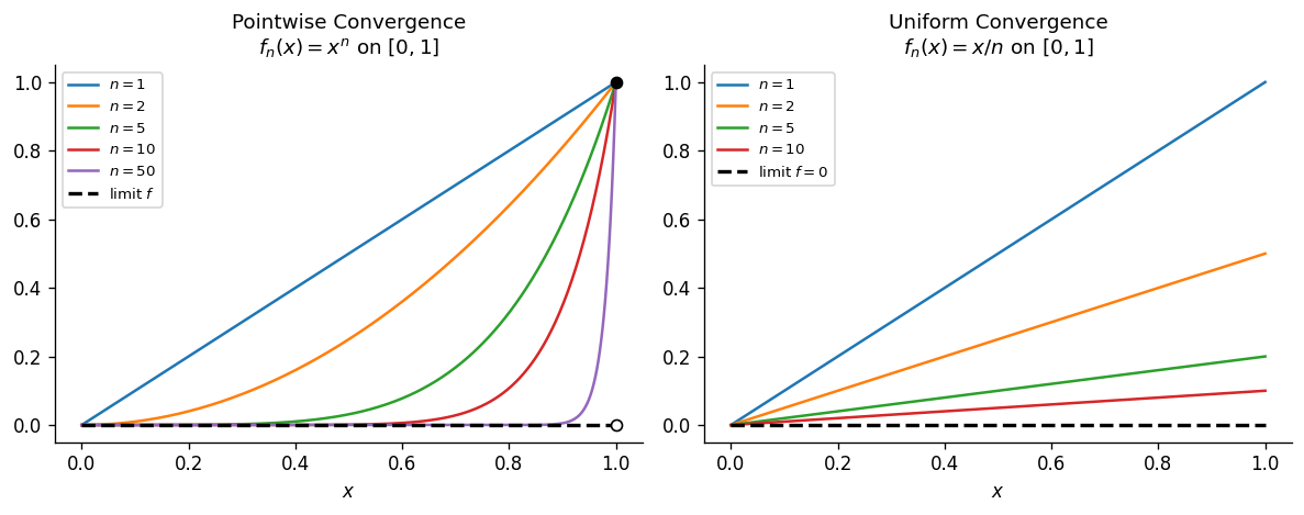
Uniform vs pointwise convergence: f_n(x)=xⁿ (pointwise, discontinuous limit) vs f_n(x)=x/n (uniform, limit=0)

Definition 4.17. A sequence \((f_n)\) in \(\mathcal{F}(X) = \{f: X \to \mathbb{R}\}\) converges uniformly to \(g\) on \(X\) if for every \(\varepsilon > 0\) there exists \(N\) such that \(|f_n(x) - g(x)| < \varepsilon\) for all \(n \ge N\) and all \(x \in X\). Equivalently, \(\|f_n - g\|_\infty \to 0\).

Pointwise convergence is much weaker: it requires only that for each fixed \(x\), the sequence \(f_n(x) \to g(x)\). The uniform limit of continuous functions is continuous, but the pointwise limit need not be.

Theorem 4.18 (Uniform limit theorem). If \(f_n: X \to Y\) are continuous and \(f_n \to g\) uniformly, then \(g\) is continuous.

Proof. Fix \(a \in X\) and \(\varepsilon > 0\). Choose \(N\) with \(d(f_N(x), g(x)) < \varepsilon/3\) for all \(x\). By continuity of \(f_N\) at \(a\), choose \(\delta > 0\) with \(d(f_N(x), f_N(a)) < \varepsilon/3\) when \(d(x,a) < \delta\). Then \(d(g(x), g(a)) \le d(g(x), f_N(x)) + d(f_N(x), f_N(a)) + d(f_N(a), g(a)) < \varepsilon\).

Remark (Interchange of limits). The uniform limit theorem is a special case of a more general principle: uniform convergence allows the interchange of limits. Specifically:

Limit interchange: If \(f_n \to g\) uniformly on a set \(S\) and \(\lim_{x \to a} f_n(x) = L_n\) exists for each \(n\), then \(\lim_n L_n\) exists and \(\lim_{x \to a} g(x) = \lim_n L_n\). That is, \(\lim_{x \to a} \lim_{n \to \infty} f_n(x) = \lim_{n \to \infty} \lim_{x \to a} f_n(x)\).
Integration: If \(f_n \to g\) uniformly on \([a,b]\), then \(\int_a^b f_n \to \int_a^b g\). This follows from \(|\int (f_n - g)| \le (b-a)\|f_n - g\|_\infty\).
Differentiation: If \(f_n \to g\) pointwise, \(f_n' \to h\) uniformly, and each \(f_n'\) is continuous, then \(g\) is differentiable and \(g' = h\). (Proved by integrating \(f_n'\) and interchanging limits on the integrals.)

Without uniformity, all three interchanges can fail. The sequence \(f_n(x) = x^n\) on \([0,1]\) converges pointwise but \(\lim \int f_n = 1 \ne 0 = \int \lim f_n\). The sequence \(f_n(x) = \sin(nx)/\sqrt{n}\) converges uniformly to 0, but \(f_n'(x) = \sqrt{n}\cos(nx)\) diverges.

Theorem 4.19 (Weierstrass M-test). Let \(f_n \in C_b(X)\) with \(\sum_{n=1}^\infty \|f_n\|_\infty < \infty\). Then \(\sum f_n\) converges uniformly to a continuous bounded function.

Proof. Let \(S_N = \sum_{n=1}^N f_n\). For \(M > N\), \(\|S_M - S_N\|_\infty \le \sum_{n=N+1}^M \|f_n\|_\infty\), which is the tail of a convergent series. So \((S_N)\) is Cauchy in \((C_b(X), d_\infty)\), hence converges.

Theorem 4.20. Let \((B(X), d_\infty)\) be the space of bounded functions \(X \to \mathbb{R}\) with supremum metric, and let \((C_b(X), d_\infty)\) be the subspace of bounded continuous functions.

\((B(X), d_\infty)\) is complete.
\(C_b(X)\) is closed in \(B(X)\), hence complete.

In particular, \((C[a,b], d_\infty)\) is complete.

Proof of (1). Let \((f_n)\) be Cauchy in \(B(X)\). For each \(x\), \(|f_n(x) - f_m(x)| \le \|f_n - f_m\|_\infty\), so \((f_n(x))\) is Cauchy in \(\mathbb{R}\), hence converges. Define \(g(x) = \lim f_n(x)\). The sequence \((\|f_n\|_\infty)\) is bounded (Cauchy sequences are bounded), say by \(M\), so \(|g(x)| \le M\) and \(g \in B(X)\). For uniform convergence: given \(\varepsilon > 0\), choose \(N\) with \(\|f_k - f_\ell\|_\infty < \varepsilon\) for \(k, \ell \ge N\). Then for \(k \ge N\): \(|f_k(x) - g(x)| = \lim_{\ell \to \infty} |f_k(x) - f_\ell(x)| \le \varepsilon\).

Proof of (2): If \(f_n \in C_b(X)\) and \(f_n \to g\) uniformly, then \(g\) is continuous by the uniform limit theorem (Theorem 4.18).

Chapter 5: Completeness and Separability

Completeness — the property that every Cauchy sequence converges — is arguably the most important structural property a metric space can possess. It is the key hypothesis in the Baire Category Theorem, the Contraction Mapping Principle, and the existence theorem for solutions of ODEs. Separability — having a countable dense subset — is the topological analogue of being “not too large.”

5.1 Cauchy Sequences and Complete Metric Spaces

Definition 5.1. A metric space \(X\) is complete if every Cauchy sequence in \(X\) converges (in \(X\)). A complete normed linear space is called a Banach space. A complete inner product space is called a Hilbert space.

Theorem 5.2 (Properties of Cauchy sequences).

Every Cauchy sequence is bounded.
Every convergent sequence is Cauchy.
If a Cauchy sequence has a convergent subsequence, then the full sequence converges (to the same limit).

Proof of (3). Let \((x_n)\) be Cauchy with subsequence \(x_{n_k} \to a\). Given \(\varepsilon > 0\), choose \(N\) so that \(d(x_k, x_\ell) < \varepsilon/2\) for \(k, \ell \ge N\), and choose \(\ell\) with \(n_\ell \ge N\) and \(d(x_{n_\ell}, a) < \varepsilon/2\). Then for \(k \ge N\): \(d(x_k, a) \le d(x_k, x_{n_\ell}) + d(x_{n_\ell}, a) < \varepsilon\).

Theorem 5.3 (Completeness and closed subsets). Let \(X\) be a complete metric space and \(A \subseteq X\). Then \(A\) is complete if and only if \(A\) is closed in \(X\).

Proof. If \(A\) is closed and \((x_n)\) is Cauchy in \(A\), then \((x_n)\) converges in \(X\) (by completeness of \(X\)) and the limit lies in \(A\) (since \(A\) is closed). Conversely, if \(A\) is complete and \(a \in A'\), choose a sequence \((x_n)\) in \(A\) with \(x_n \to a\). Then \((x_n)\) is Cauchy, hence converges in \(A\), so \(a \in A\), proving \(A' \subseteq A\).

Remark. Completeness is not a topological invariant: \(\mathbb{R}\) is complete but homeomorphic to \((0,1)\), which is not complete (the Cauchy sequence \(1/n\) has no limit in \((0,1)\)). The homeomorphism \(f(x) = \tan(\pi x - \pi/2): (0,1) \to \mathbb{R}\) maps incomplete to complete. Thus completeness depends on the specific metric, not just the topology. However, completeness is preserved by biLipschitz equivalence: if \(f: (X,d) \to (Y,\rho)\) is biLipschitz and \(X\) is complete, then \(Y\) is complete (Cauchy sequences in \(Y\) pull back to Cauchy sequences in \(X\)).

Theorem 5.3a (Cantor's characterization of completeness). A metric space \(X\) is complete if and only if it satisfies the nested closed sets property: whenever \(C_1 \supseteq C_2 \supseteq \cdots\) are nonempty closed sets with \(\operatorname{diam}(C_n) \to 0\), then \(\bigcap_{n=1}^\infty C_n\) is a single point.

Proof. (\(\Rightarrow\)): Given nested closed sets with diameters tending to 0, choose \(x_n \in C_n\). For \(n, m \ge N\), both \(x_n, x_m \in C_N\), so \(d(x_n, x_m) \le \operatorname{diam}(C_N) \to 0\). Thus \((x_n)\) is Cauchy, hence converges to some \(a \in X\). Since \(x_m \in C_n\) for all \(m \ge n\) and \(C_n\) is closed, \(a \in C_n\) for all \(n\). So \(a \in \bigcap C_n\). Uniqueness follows from \(\operatorname{diam}(\bigcap C_n) \le \operatorname{diam}(C_n) \to 0\).

(\(\Leftarrow\)): Let \((x_n)\) be Cauchy. Define \(C_n = \overline{\{x_k : k \ge n\}}\). These are nonempty, closed, nested, and \(\operatorname{diam}(C_n) = \operatorname{diam}(\{x_k : k \ge n\}) \to 0\) since the sequence is Cauchy. The unique point \(a \in \bigcap C_n\) is the limit: for each \(\varepsilon > 0\), choose \(N\) with \(\operatorname{diam}(C_N) < \varepsilon\), then for \(n \ge N\), \(d(x_n, a) \le \operatorname{diam}(C_N) < \varepsilon\).

Remark. Cantor's characterization is useful for proving completeness without explicitly exhibiting the limit of a Cauchy sequence. It also reveals the relationship between completeness and compactness: in a complete space, nested closed sets with diameters tending to 0 have nonempty intersection (a single point). In a compact space, any family of closed sets with the finite intersection property has nonempty intersection (Theorem 6.5). Compactness strengthens completeness by removing the "diameters to 0" requirement.

Example 5.2a (Incomplete spaces). \((\mathbb{Q}, |\cdot|)\) is not complete: the sequence of rational approximations to \(\sqrt{2}\) is Cauchy but has no rational limit. The space \(C_c(\mathbb{R})\) of compactly supported continuous functions under \(\|\cdot\|_\infty\) is not complete: the sequence \(f_n(x) = e^{-x^2} \max\{1 - |x|/n, 0\}\) is Cauchy in \(\|\cdot\|_\infty\) but converges to \(e^{-x^2}\), which is not compactly supported. Open subsets of complete spaces are generally not complete: \((0,1)\) is open in the complete space \(\mathbb{R}\).

Example 5.2b (The Baire space). The Baire space \(\mathbb{N}^{\mathbb{N}}\) is the set of all sequences of natural numbers, equipped with the metric \[ d(\alpha, \beta) = \begin{cases} 0 & \text{if } \alpha = \beta, \\ 2^{-\min\{n : \alpha(n) \ne \beta(n)\}} & \text{otherwise.} \end{cases} \]

This is a complete ultrametric space. To verify completeness: if \((\alpha_k)\) is Cauchy, then for each \(n\), there exists \(K\) such that the first \(n\) terms of \(\alpha_k\) agree for all \(k \ge K\). Define \(\beta(n) = \lim_k \alpha_k(n)\) (eventually constant). Then \(\alpha_k \to \beta\) in the metric.

The Baire space is homeomorphic to the irrational numbers \(\mathbb{R} \setminus \mathbb{Q}\) (via continued fraction expansion: each irrational has a unique continued fraction \([a_0; a_1, a_2, \ldots]\) with \(a_i \in \mathbb{N}\) for \(i \ge 1\), and this correspondence is a homeomorphism). Since \(\mathbb{N}^{\mathbb{N}}\) is complete, this gives an indirect proof that the irrationals are completely metrizable — they admit a complete metric inducing the same topology, even though the usual metric inherited from \(\mathbb{R}\) is not complete. The Baire space plays a fundamental role in descriptive set theory, where it serves as the “canonical” Polish space of dimension zero.

Remark (Polish spaces). A Polish space is a separable, completely metrizable topological space. The Baire Category Theorem applies to all Polish spaces (since they admit a complete metric). Important examples include \(\mathbb{R}^n\), \(C[0,1]\), the Cantor set \(2^{\mathbb{N}}\), the Baire space \(\mathbb{N}^{\mathbb{N}}\), and the irrationals \(\mathbb{R} \setminus \mathbb{Q}\). A useful theorem of Alexandrov states that a subspace of a complete metric space is completely metrizable if and only if it is a \(G_\delta\) subset. Since the irrationals are \(G_\delta\) in \(\mathbb{R}\) (Example 8.5a), this gives another proof that they are completely metrizable. Conversely, \(\mathbb{Q}\) is \(F_\sigma\) but not \(G_\delta\) in \(\mathbb{R}\) (by the BCT --- see Section 8.6), confirming that \(\mathbb{Q}\) is not completely metrizable.

5.2 Completeness of Key Spaces

Theorem 5.4. \(\mathbb{R}\) is complete (the Completeness Axiom). More generally, \(\mathbb{R}^n\) is complete under any \(\ell^p\) norm.

Proof for \(\mathbb{R}\). Let \((x_n)\) be Cauchy in \(\mathbb{R}\). By Theorem 5.2, \((x_n)\) is bounded, say \(|x_n| \le M\). Define \(L = \sup\{x_n : n \ge 1\}\). We claim \(x_n \to L\). Given \(\varepsilon > 0\), choose \(N\) with \(|x_n - x_m| < \varepsilon/2\) for \(n, m \ge N\). Since \(L - \varepsilon/2\) is not an upper bound of \(\{x_n : n \ge N\}\) (for otherwise \(L\) could be decreased), there exists \(n_0 \ge N\) with \(x_{n_0} > L - \varepsilon/2\). Then for \(n \ge N\): \(x_n \ge x_{n_0} - |x_n - x_{n_0}| > L - \varepsilon/2 - \varepsilon/2 = L - \varepsilon\), and \(x_n \le L\). So \(|x_n - L| < \varepsilon\).

Theorem 5.4a (Bolzano--Weierstrass). Every bounded sequence in \(\mathbb{R}^n\) has a convergent subsequence.

Proof for \(\mathbb{R}\). Let \((x_n)\) be bounded, say \(x_n \in [a,b]\). Bisect: at least one of \([a, (a+b)/2]\) or \([(a+b)/2, b]\) contains infinitely many terms; call this interval \(I_1\) and pick \(x_{n_1} \in I_1\). Repeat to get nested intervals \(I_1 \supseteq I_2 \supseteq \cdots\) with \(|I_k| = (b-a)/2^k \to 0\) and \(x_{n_k} \in I_k\). By Cantor's Intersection Theorem, \(\bigcap I_k = \{L\}\), and \(|x_{n_k} - L| \le |I_k| \to 0\).

For \(\mathbb{R}^n\): extract a subsequence converging in the first coordinate, then a further subsequence converging in the second coordinate, etc. After \(n\) extractions, the final subsequence converges in all coordinates.

Theorem 5.4b (Completeness of \(\mathbb{R}^n\)). \(\mathbb{R}^n\) is complete under any \(\ell^p\) norm.

Proof. A sequence \((\mathbf{x}_k)\) in \(\mathbb{R}^n\) is Cauchy if and only if each coordinate sequence \((x_k^{(j)})_{k \ge 1}\) is Cauchy in \(\mathbb{R}\) (this follows from the equivalence of all norms on \(\mathbb{R}^n\)). By completeness of \(\mathbb{R}\), each coordinate converges. The limit \(\mathbf{x} = (\lim x_k^{(1)}, \ldots, \lim x_k^{(n)})\) satisfies \(\|\mathbf{x}_k - \mathbf{x}\|_p \to 0\) because convergence in each coordinate implies convergence in any \(\ell^p\) norm (again by norm equivalence).

Theorem 5.5. Every finite-dimensional normed linear space is complete (hence is a Banach space).

Proof. Let \(U\) have basis \(\{u_1, \ldots, u_n\}\) with isomorphism \(F: \mathbb{R}^n \to U\). Both \(F\) and \(F^{-1}\) are Lipschitz (Theorem 4.15). If \((x_k)\) is Cauchy in \(U\), then \((F^{-1}(x_k))\) is Cauchy in \(\mathbb{R}^n\), hence convergent (since \(\mathbb{R}^n\) is complete). If \(s = \lim F^{-1}(x_k)\), then \(x_k = F(F^{-1}(x_k)) \to F(s)\).

Theorem 5.6. The sequence spaces \((\ell^1, d_1)\), \((\ell^2, d_2)\), and \((\ell^\infty, d_\infty)\) are all complete. More generally, \((\ell^p, d_p)\) is complete for every \(1 \le p \le \infty\).

Remark. To even define \(\ell^p\), one needs the Minkowski inequality \(\|a + b\|_p \le \|a\|_p + \|b\|_p\), which ensures the triangle inequality holds. For \(p = 1\) and \(p = \infty\) this is elementary; for \(1 < p < \infty\) it requires Hölder's inequality first. Recall that the \(\ell^p\) norm is \(\|a\|_p = \left(\sum_{k=1}^\infty |a_k|^p\right)^{1/p}\) for \(1 \le p < \infty\) and \(\|a\|_\infty = \sup_k |a_k|\). The spaces form a nested chain: \(\ell^1 \subsetneq \ell^2 \subsetneq \cdots \subsetneq \ell^\infty\), with \(\|a\|_q \le \|a\|_p\) for \(p \le q\). The sequence \(a_k = 1/k\) lies in \(\ell^2\) but not \(\ell^1\), confirming strictness of the inclusions.

The proof strategy for all \(\ell^p\) spaces is the same three-step pattern, sometimes called the “standard completeness argument”:

Coordinatewise convergence: show the Cauchy sequence converges in each coordinate.
Membership: show the coordinatewise limit actually belongs to \(\ell^p\).
Norm convergence: show convergence holds in the \(\ell^p\) norm, not just coordinatewise.

This strategy is used repeatedly in functional analysis whenever proving completeness of a function space.

Proof for \(\ell^1\). Let \((a^{(n)})\) be Cauchy in \(\ell^1\), where \(a^{(n)} = (a^{(n)}_k)_{k \ge 1}\). For each fixed \(k\), \(|a^{(n)}_k - a^{(m)}_k| \le \|a^{(n)} - a^{(m)}\|_1 \to 0\), so \((a^{(n)}_k)_n\) converges in \(\mathbb{R}\). Let \(b_k = \lim_n a^{(n)}_k\). Since \((\|a^{(n)}\|_1)\) is bounded (Cauchy sequences are bounded), say by \(M\), we get \(\sum_{k=1}^K |b_k| = \lim_n \sum_{k=1}^K |a^{(n)}_k| \le M\) for all \(K\), so \(b \in \ell^1\). For convergence: given \(\varepsilon > 0\), choose \(N\) with \(\|a^{(n)} - a^{(m)}\|_1 < \varepsilon\) for \(n, m \ge N\). Then \(\sum_{k=1}^K |a^{(n)}_k - b_k| = \lim_{m \to \infty} \sum_{k=1}^K |a^{(n)}_k - a^{(m)}_k| \le \varepsilon\). Letting \(K \to \infty\) gives \(\|a^{(n)} - b\|_1 \le \varepsilon\).

Proof for general \(\ell^p\) (\(1 < p < \infty\)). Let \((a^{(n)})\) be Cauchy in \(\ell^p\).

Step 1 (Coordinatewise convergence): For each fixed \(k\), \(|a^{(n)}_k - a^{(m)}_k| \le \|a^{(n)} - a^{(m)}\|_p \to 0\), so \(b_k := \lim_n a^{(n)}_k\) exists.

Step 2 (Membership): Fix \(\varepsilon > 0\) and choose \(N\) with \(\|a^{(n)} - a^{(m)}\|_p < \varepsilon\) for \(n, m \ge N\). For any finite \(K\):

\[ \left(\sum_{k=1}^K |a^{(n)}_k - b_k|^p\right)^{1/p} = \lim_{m \to \infty} \left(\sum_{k=1}^K |a^{(n)}_k - a^{(m)}_k|^p\right)^{1/p} \le \varepsilon. \]

Letting \(K \to \infty\): \(\|a^{(n)} - b\|_p \le \varepsilon\) for \(n \ge N\). In particular, \(a^{(n)} - b \in \ell^p\), so \(b = a^{(n)} - (a^{(n)} - b) \in \ell^p\) (since \(\ell^p\) is a vector space).

Step 3 (Norm convergence): The estimate \(\|a^{(n)} - b\|_p \le \varepsilon\) for \(n \ge N\) is exactly convergence in the \(\ell^p\) norm.

Proof for \(\ell^\infty\). Let \((a^{(n)})\) be Cauchy in \(\ell^\infty\). Coordinatewise limits \(b_k = \lim_n a^{(n)}_k\) exist as before. Boundedness: \((\|a^{(n)}\|_\infty)\) is bounded, say by \(M\), so \(|b_k| = \lim_n |a^{(n)}_k| \le M\), giving \(b \in \ell^\infty\). Norm convergence: for \(n \ge N\), \(|a^{(n)}_k - b_k| = \lim_{m \to \infty} |a^{(n)}_k - a^{(m)}_k| \le \varepsilon\) for all \(k\), giving \(\|a^{(n)} - b\|_\infty \le \varepsilon\).

Remark (The spaces \(c\) and \(c_0\)). Two important closed subspaces of \(\ell^\infty\) are:

\(c = \{(a_n) \in \ell^\infty : \lim a_n \text{ exists}\}\), the space of convergent sequences.
\(c_0 = \{(a_n) \in \ell^\infty : \lim a_n = 0\}\), the space of sequences converging to zero.

Both are closed subspaces of \(\ell^\infty\) (the sup-norm limit of convergent sequences is convergent, and similarly for null sequences), hence complete Banach spaces. Neither is separable's converse: \(\ell^\infty\) itself is not separable (the uncountably many sequences of 0s and 1s are mutually at distance 1), but \(c_0\) is separable (the sequences with finitely many nonzero rational entries form a countable dense subset). This distinction matters: separable Banach spaces have better structural properties --- for instance, the dual of \(c_0\) is \(\ell^1\), and the dual of \(\ell^1\) is \(\ell^\infty\), forming a clean duality chain \(c_0 \subset c \subset \ell^\infty\) with \(c_0^* = \ell^1\) and \(\ell^{1*} = \ell^\infty\).

Theorem 5.7. \((C[a,b], d_\infty)\) is complete, but \((C[a,b], d_1)\) and \((C[a,b], d_2)\) are not complete.

Proof of incompleteness of \(d_1\). Consider \(f_n: [-1,1] \to \mathbb{R}\) given by \(f_n(x) = x^{1/(2n-1)}\). The sequence \((f_n)\) is Cauchy in \(d_1\), but if it converged, the limit would have to be the sign function \(g(x) = 1\) for \(x > 0\), \(g(x) = -1\) for \(x < 0\), which is discontinuous.

Example 5.7c (Incompleteness under \(d_1\) and \(d_2\)). The space \(C[-1,1]\) under the \(d_1\) metric is not complete. Consider the sequence of continuous functions \[ f_n(x) = \begin{cases} -1, & x \le -1/n, \\ nx, & -1/n \le x \le 1/n, \\ 1, & x \ge 1/n. \end{cases} \]

One verifies \(\|f_n - f_m\|_1 \to 0\) as \(n, m \to \infty\), so \((f_n)\) is Cauchy in \(d_1\). The pointwise limit is the sign function \(\operatorname{sgn}(x)\), which is discontinuous, so the sequence has no limit in \(C[-1,1]\). The same construction works for \(d_2\). The completions of \((C[a,b], d_p)\) are the \(L^p\) spaces — a topic developed in PMATH 450 (Lebesgue Integration).

Example 5.8. The closed unit ball in \((C[0,1], d_\infty)\) is not compact. The sequence \(f_n(x) = x^n\) satisfies \(\|f_n\|_\infty = 1\), so each \(f_n\) lies in the closed unit ball. The pointwise limit is \(g(x) = 0\) for \(x < 1\), \(g(1) = 1\), which is discontinuous. Hence no subsequence converges uniformly, and the ball is not sequentially compact.

5.3 The Uniform Limit Theorem and Series of Functions

The interplay between completeness and uniform convergence yields powerful results about series of functions.

Theorem 5.7a (Completeness of \(C_b(X)\) --- general version). Let \((X,d)\) be any metric space and \((Y, d_Y)\) a complete metric space. The space of bounded continuous functions \(C_b(X, Y)\) with the supremum metric \(d_\infty(f,g) = \sup_{x \in X} d_Y(f(x), g(x))\) is complete.

Proof. If \((f_n)\) is Cauchy in \(C_b(X,Y)\), then for each \(x\), \((f_n(x))\) is Cauchy in \(Y\), hence converges to some \(g(x)\). The limit \(g\) is bounded (since \(\|f_n\|_\infty\) is bounded, being a Cauchy sequence of reals) and continuous (by the uniform limit theorem). The convergence is uniform by the same argument as in Theorem 4.20.

Remark (Pointwise vs. uniform convergence). The distinction between pointwise and uniform convergence is critical throughout analysis:

Pointwise convergence of \(f_n \to g\) means: for each \(x\) and \(\varepsilon > 0\), there exists \(N(x,\varepsilon)\) with \(|f_n(x) - g(x)| < \varepsilon\) for \(n \ge N\). The \(N\) may depend on \(x\).
Uniform convergence means: for each \(\varepsilon > 0\), there exists \(N(\varepsilon)\) (independent of \(x\)) with \(\sup_x |f_n(x) - g(x)| < \varepsilon\) for \(n \ge N\).

Uniform convergence preserves continuity, boundedness, and (on compact domains) integrability. Pointwise convergence preserves none of these in general. The sequence \(f_n(x) = x^n\) on \([0,1]\) converges pointwise to a discontinuous limit, illustrating the failure.

Example 5.7b (Series convergence). The Weierstrass M-test applies to show that \(f(x) = \sum_{n=0}^\infty \frac{x^n}{n!}\) converges uniformly on any \([-R, R]\) (since \(\sum R^n/n! < \infty\)), and \(g(x) = \sum_{n=1}^\infty \frac{\sin(nx)}{n^2}\) converges uniformly on \(\mathbb{R}\) (since \(\sum 1/n^2 < \infty\)), yielding a continuous function. However, \(\sum \frac{\sin(nx)}{n}\) converges pointwise but not uniformly.

5.4 Separability

Definition 5.9. A metric space \(X\) is separable if it has a finite or countable dense subset. A basis for the topology on \(X\) is a collection \(\mathcal{B}\) of open sets such that every open set is a union of members of \(\mathcal{B}\). A space is second-countable if it has a countable basis.

Theorem 5.10.

A metric space is separable if and only if it is second-countable. If \(D\) is a countable dense set, then \(\{B(q, 1/n) : q \in D, n \ge 1\}\) is a countable basis.
Every subspace of a separable metric space is separable.
If every infinite subset of \(X\) has a limit point, then \(X\) is separable.

Proof of (2) (Separability of subspaces). Let \(X\) be separable with countable dense set \(D\), and let \(Y \subseteq X\). By (1), \(X\) has a countable basis \(\mathcal{B} = \{B_n\}\). The collection \(\mathcal{B}_Y = \{B_n \cap Y : B_n \cap Y \ne \emptyset\}\) is a countable basis for the subspace topology on \(Y\). Picking one point \(q_n\) from each nonempty \(B_n \cap Y\) gives a countable dense subset of \(Y\).

Proof of (3). If \(X\) is not separable, for any countable set \(\{x_1, x_2, \ldots\}\), there exists \(\varepsilon > 0\) and a point outside all \(B(x_i, \varepsilon)\). This lets us greedily construct an infinite set of points mutually at distance \(\ge \varepsilon\), which has no limit point --- contradiction.

Remark (Separability and cardinality). Separability is a powerful "size constraint" on a metric space. Any separable metric space has at most \(\mathfrak{c} = 2^{\aleph_0}\) points. This follows because a point \(x\) is determined by the sequence of distances \((d(x, q_n))_{n \ge 1}\) to the elements of a countable dense set \(\{q_n\}\), and each such sequence lies in \(\mathbb{R}^{\mathbb{N}}\), which has cardinality \(\mathfrak{c}\). Consequently, any metric space with more than \(\mathfrak{c}\) points is automatically non-separable.

Theorem 5.11 (Lindelöf Property). Every second-countable (hence separable) metric space has the Lindelöf property: every open cover has a countable subcover.

Proof. Let \(\mathcal{B} = \{B_n\}_{n \ge 1}\) be a countable basis and \(\mathcal{U}\) an open cover. For each \(x\), choose \(U_x \in \mathcal{U}\) with \(x \in U_x\), then choose \(B_{n_x} \in \mathcal{B}\) with \(x \in B_{n_x} \subseteq U_x\). The set of indices \(\{n_x : x \in X\}\) is a countable subset of \(\mathbb{N}\). For each such index \(n\), choose one \(U_n \in \mathcal{U}\) with \(B_n \subseteq U_n\). Then \(\{U_n\}\) is a countable subcover.

Proof of (1). If \(D\) is countable and dense, then \(\mathcal{B} = \{B(q, 1/n) : q \in D, n \ge 1\}\) is countable. For any open \(U\) and \(x \in U\), choose \(r > 0\) with \(B(x,r) \subseteq U\), then \(q \in D\) with \(d(q,x) < r/2\), then \(n\) with \(1/n < r/2\). Then \(x \in B(q, 1/n) \subseteq B(x,r) \subseteq U\). Conversely, if \(\{B_n\}\) is a countable basis, pick one point from each nonempty \(B_n\) to get a countable dense set.

Example 5.11.

\(\mathbb{R}^n\) is separable (\(\mathbb{Q}^n\) is a countable dense subset).
\((C[a,b], d_\infty)\) is separable (polynomials with rational coefficients are countable and dense, by the Weierstrass Approximation Theorem).
\((\ell^p, d_p)\) is separable for \(1 \le p < \infty\): the sequences with finitely many nonzero rational entries form a countable dense subset.
\((\ell^\infty, d_\infty)\) is not separable: for each subset \(A \subseteq \mathbb{N}\), the characteristic function \(\chi_A\) satisfies \(\|\chi_A - \chi_B\|_\infty = 1\) when \(A \ne B\), giving an uncountable set of points mutually at distance 1.
\((B[a,b], d_\infty)\) is not separable, for the same reason with characteristic functions of subsets of \([a,b]\).

Theorem 5.12 (Lindelöf property). In a second-countable (equivalently, separable metric) space, every open cover has a countable subcover.

Chapter 6: Compactness

Compactness is arguably the single most important topological property in analysis. It is the correct generalization of “closed and bounded” that works in all metric spaces. Compact sets have the remarkable property that every sequence has a convergent subsequence, which makes them indispensable in optimization, approximation theory, and differential equations.

6.1 Open Covers and the Definition of Compactness

Definition 6.1. Let \(X\) be a metric space and \(A \subseteq X\). An open cover of \(A\) is a collection \(\mathcal{S}\) of open sets whose union contains \(A\). A subcover is a subcollection that still covers \(A\). We say \(A\) is compact if every open cover of \(A\) has a finite subcover.

Theorem 6.2. If \(A\) is compact, then \(A\) is closed and bounded.

Proof. To show \(A\) is closed: let \(a \in A^c\). For each \(x \in A\), let \(r_x = d(a,x)/2\) and set \(V_x = B(x, r_x)\). The \(\{V_x\}\) cover \(A\), so finitely many suffice: \(A \subseteq V_{x_1} \cup \cdots \cup V_{x_n}\). Then \(B(a, r) \subseteq A^c\) where \(r = \min\{r_{x_1}, \ldots, r_{x_n}\}\). To show \(A\) is bounded: \(\{B(a, n)\}_{n \ge 1}\) covers \(A\), so finitely many suffice, giving \(A \subseteq B(a, N)\) for some \(N\).

The converse fails in general — the closed unit ball in \(C[0,1]\) is closed and bounded but not compact. More precisely:

Example 6.2a. In an infinite-dimensional normed space, the closed unit ball is never compact. In \((\ell^2, \|\cdot\|_2)\), the standard basis vectors \(e_n\) satisfy \(\|e_n\|_2 = 1\) and \(\|e_m - e_n\|_2 = \sqrt{2}\) for \(m \ne n\), so the sequence \((e_n)\) has no convergent subsequence. In \((C[0,1], \|\cdot\|_\infty)\), the functions \(f_n(x) = x^n\) all lie in the unit ball, but converge pointwise to a discontinuous limit, so no subsequence converges uniformly. This failure of the Heine--Borel theorem in infinite dimensions is what makes the Arzela--Ascoli theorem essential --- it identifies the additional condition (equicontinuity) needed for compactness in function spaces.

Theorem 6.3. Let \(X\) be compact and \(A \subseteq X\) closed. Then \(A\) is compact.

Proof. If \(\mathcal{S}\) covers \(A\), then \(\mathcal{S} \cup \{A^c\}\) covers \(X\). Extract a finite subcover of \(X\); removing \(A^c\) (if present) gives a finite subcover of \(A\).

Theorem 6.4. Compactness is intrinsic: \(A \subseteq P \subseteq X\) is compact in \(P\) iff it is compact in \(X\).

Theorem 6.5 (Cantor's Intersection Theorem). Let \(X\) be a compact metric space and \(C_1 \supseteq C_2 \supseteq C_3 \supseteq \cdots\) a decreasing sequence of nonempty closed sets. Then \(\bigcap_{n=1}^\infty C_n \ne \emptyset\). If additionally \(\operatorname{diam}(C_n) \to 0\), the intersection is a single point.

Proof. If the intersection were empty, then \(\{C_n^c\}\) would be an open cover of \(X\) with no finite subcover (since \(C_1^c \cup \cdots \cup C_n^c = C_n^c \ne X\) because \(C_n \ne \emptyset\)), contradicting compactness.

6.2 Sequential Compactness and Total Boundedness

Definition 6.6. A metric space \(X\) is totally bounded if for every \(\varepsilon > 0\) there exist finitely many points \(a_1, \ldots, a_n \in X\) such that \(X = \bigcup_{i=1}^n B(a_i, \varepsilon)\). Such a set \(\{a_1, \ldots, a_n\}\) is called an \(\varepsilon\)-net.

Remark. Totally bounded implies bounded (take \(\varepsilon = 1\) and use the triangle inequality), but the converse fails: the unit ball of \(\ell^2\) is bounded but not totally bounded (the standard basis vectors are mutually at distance \(\sqrt{2}\)).

Proposition 6.6a (Properties of total boundedness).

Every subset of a totally bounded space is totally bounded.
A metric space is totally bounded if and only if every sequence has a Cauchy subsequence.
If \(f: X \to Y\) is uniformly continuous and \(X\) is totally bounded, then \(f(X)\) is totally bounded.
Finite products of totally bounded spaces are totally bounded.

Proof of (2). (\(\Rightarrow\)): Given a sequence \((x_n)\), cover \(X\) by finitely many balls of radius 1. One ball contains infinitely many terms; extract a subsequence. Cover by balls of radius \(1/2\); one ball contains infinitely many terms of this subsequence; extract a further subsequence. Continue. The diagonal subsequence satisfies: for terms beyond the \(k\)-th extraction, consecutive terms lie within a ball of radius \(1/k\), so it is Cauchy.

(\(\Leftarrow\)): If \(X\) is not totally bounded, there exists \(\varepsilon > 0\) and an infinite sequence \((a_n)\) with \(d(a_n, a_m) \ge \varepsilon\) for \(n \ne m\) (constructed greedily). No subsequence of \((a_n)\) is Cauchy, contradicting the hypothesis.

Example 6.6b. Total boundedness versus boundedness in function spaces:

In \(\mathbb{R}^n\), bounded and totally bounded are equivalent (by Heine--Borel, both are equivalent to having compact closure).
In \(\ell^2\), the set \(S = \{e_n/n : n \ge 1\}\) is totally bounded (it converges to 0, so every sequence in \(S\) has a Cauchy subsequence). But the set \(\{e_n : n \ge 1\}\) is bounded (\(\|e_n\| = 1\)) but not totally bounded.
In \(C[0,1]\), the set \(\{f_n(x) = x^n/n : n \ge 1\}\) is totally bounded (since \(\|f_n\|_\infty = 1/n \to 0\)), while \(\{x^n : n \ge 1\}\) is bounded but not totally bounded (the pointwise limit is discontinuous, so Arzela--Ascoli fails).

Theorem 6.7 (Equivalences of Compactness). For a metric space \(X\), the following are equivalent:

\(X\) is compact (every open cover has a finite subcover).
\(X\) has the finite intersection property on closed sets: if every finite sub-collection of a collection of closed sets has nonempty intersection, so does the whole collection.
Every sequence in \(X\) has a convergent subsequence (sequential compactness).
Every infinite subset of \(X\) has a limit point (Bolzano--Weierstrass property).
\(X\) is complete and totally bounded.

Proof (Key directions).

(1)\(\Rightarrow\)(2): By contrapositive via complements. (2)\(\Rightarrow\)(3): Given \((x_n)\), the sets \(A_m = \overline{\{x_n : n > m\}}\) satisfy the FIP; choose \(a \in \bigcap A_m\) and build a subsequence converging to \(a\). (3)\(\Rightarrow\)(4): Choose a sequence of distinct points in the infinite set and extract a convergent subsequence.

(4)\(\Rightarrow\)(5): For completeness: if \((x_n)\) is Cauchy, the set \(\{x_n\}\) either has a repeated term (giving a constant convergent subsequence) or is infinite, hence has a limit point, so a subsequence converges, so the Cauchy sequence converges. For total boundedness: if \(X\) is not totally bounded, there exists \(\varepsilon > 0\) such that no finite \(\varepsilon\)-net covers \(X\). Construct inductively \(a_1, a_2, \ldots\) with \(d(a_n, a_m) \ge \varepsilon\) for \(m \ne n\). Then \(\{a_n\}\) is infinite with no limit point — contradiction.

(5)\(\Rightarrow\)(1): Suppose \(X\) is complete and totally bounded but not compact. Choose an open cover \(\mathcal{S}\) with no finite subcover. Cover \(X\) by finitely many balls of radius 1. At least one ball \(U_1 = B(a_1, 1)\) has no finite subcover from \(\mathcal{S}\). Cover \(X\) by balls of radius \(1/2\); choose \(U_2 = B(a_2, 1/2)\) with \(U_1 \cap U_2\) having no finite subcover. Continue to get nested intersections \(\bigcap_{k=1}^n U_k \ne \emptyset\) with no finite subcover. Pick \(x_n \in \bigcap_{k=1}^n U_k\). Since \(x_k, x_\ell \in U_m = B(a_m, 1/m)\) for \(k, \ell \ge m\), the sequence \((x_n)\) is Cauchy, hence converges to some \(a\). Choose \(U \in \mathcal{S}\) with \(a \in U\) and \(B(a,r) \subseteq U\). For large \(m\), \(U_m \subseteq B(a,r) \subseteq U\), so \(\{U\}\) finitely covers \(U_m\) — contradiction.

The equivalence (1) \(\Leftrightarrow\) (5) decomposes compactness into completeness (limits exist) and total boundedness (the space is “almost finite” at every scale). This decomposition is the key to understanding why compactness fails in infinite dimensions: while \(\ell^2\) is complete, the closed unit ball is bounded but not totally bounded (the standard basis vectors \(e_n\) are mutually at distance \(\sqrt{2}\), so no finite \(\varepsilon\)-net exists for \(\varepsilon < \sqrt{2}/2\)).

Remark (One-point compactification). Every locally compact metric space \(X\) can be made compact by adding a single "point at infinity." The one-point compactification \(X^+ = X \cup \{\infty\}\) is topologized by declaring the open sets to be the open sets of \(X\) together with the sets \(\{\infty\} \cup (X \setminus K)\) for compact \(K \subseteq X\). Then \(X^+\) is compact, and \(X\) embeds as an open dense subspace.

Important examples:

The one-point compactification of \(\mathbb{R}\) is homeomorphic to the circle \(S^1\) (via stereographic projection).
The one-point compactification of \(\mathbb{R}^n\) is homeomorphic to the sphere \(S^n\).
The one-point compactification of the discrete space \(\mathbb{N}\) is homeomorphic to the convergent sequence \(\{0, 1, 1/2, 1/3, \ldots\}\) with the usual metric.

The one-point compactification is a topological construction: in general, \(X^+\) may not be metrizable. However, when \(X\) is locally compact, separable, and metrizable (a "locally compact Polish space"), the one-point compactification is metrizable. For spaces that are already compact, the one-point compactification simply adds an isolated point.

Theorem 6.7a (Products of compact spaces). If \(X\) and \(Y\) are compact metric spaces, then \(X \times Y\) is compact (in any product metric).

Proof. Let \((x_n, y_n)\) be a sequence in \(X \times Y\). By compactness of \(X\), there is a subsequence \(x_{n_k} \to x\). By compactness of \(Y\), there is a further subsequence \(y_{n_{k_\ell}} \to y\). Then \((x_{n_{k_\ell}}, y_{n_{k_\ell}}) \to (x,y)\) in the product metric.

Theorem 6.8 (Heine--Borel). A subset of \(\mathbb{R}^n\) is compact if and only if it is closed and bounded.

Proof. Compact implies closed and bounded (Theorem 6.2). Conversely, if \(A \subseteq \mathbb{R}^n\) is closed and bounded, it is a closed subset of \([-M,M]^n\) for some \(M\). The box \([-M,M]^n\) is complete (closed in \(\mathbb{R}^n\)) and totally bounded (cover by cubes of side \(\varepsilon/\sqrt{n}\)), hence compact. A closed subset of a compact space is compact.

6.3 Compactness and Continuity

The theorems in this section are among the most frequently used consequences of compactness.

Theorem 6.9. Let \(f: X \to Y\) be continuous with \(X\) compact. Then \(f(X)\) is compact.

Proof. Let \(\mathcal{T}\) be an open cover of \(f(X)\). Then \(\{f^{-1}(V) : V \in \mathcal{T}\}\) is an open cover of \(X\). Extract a finite subcover \(\{f^{-1}(V_1), \ldots, f^{-1}(V_n)\}\). Then \(\{V_1, \ldots, V_n\}\) covers \(f(X)\).

Theorem 6.10 (Extreme Value Theorem). If \(X\) is compact and \(f: X \to \mathbb{R}\) is continuous, then \(f\) attains its maximum and minimum.

Theorem 6.11. If \(X\) is compact and \(f: X \to Y\) is a continuous bijection, then \(f\) is a homeomorphism.

Proof. We must show \(f^{-1}\) is continuous, i.e., \(f\) maps closed sets to closed sets. If \(A \subseteq X\) is closed, then \(A\) is compact (closed subset of compact), so \(f(A)\) is compact (continuous image of compact), hence \(f(A)\) is closed.

Example 6.12. Compactness is essential: the map \(f: [0, 2\pi) \to S^1\) given by \(f(t) = e^{it}\) is a continuous bijection, but not a homeomorphism because \([0, 2\pi)\) is not compact.

Theorem 6.13 (Lebesgue Number Lemma). If \(X\) is compact and \(\mathcal{S}\) is an open cover of \(X\), there exists \(\lambda > 0\) (a Lebesgue number) such that every ball \(B(a, \lambda)\) is contained in some member of \(\mathcal{S}\).

Proof. Suppose no Lebesgue number exists. Then for each \(n \ge 1\), there exists \(x_n\) such that \(B(x_n, 1/n)\) is not contained in any member of \(\mathcal{S}\). By compactness, a subsequence \(x_{n_k} \to a\). Choose \(U \in \mathcal{S}\) with \(a \in U\) and \(r > 0\) with \(B(a,r) \subseteq U\). For large \(k\), \(d(x_{n_k}, a) < r/2\) and \(1/n_k < r/2\), so \(B(x_{n_k}, 1/n_k) \subseteq B(a,r) \subseteq U\) --- contradiction.

Theorem 6.14. If \(X\) is compact and \(f: X \to Y\) is continuous, then \(f\) is uniformly continuous.

Proof. Given \(\varepsilon > 0\), for each \(x \in X\), choose \(\delta_x > 0\) with \(d(x,y) < \delta_x \implies d(f(x), f(y)) < \varepsilon/2\). The balls \(\{B(x, \delta_x/2)\}\) cover \(X\). Let \(\lambda\) be the Lebesgue number for this cover (Theorem 6.13). If \(d(x,y) < \lambda\), then both \(x\) and \(y\) lie in some ball \(B(z, \delta_z/2)\), so \(d(x,z) < \delta_z/2 < \delta_z\) and \(d(y,z) < \delta_z/2 < \delta_z\), giving \(d(f(x), f(y)) \le d(f(x), f(z)) + d(f(z), f(y)) < \varepsilon\).

Remark. The converse of Theorem 6.14 is false: the function \(f(x) = x\) on \(\mathbb{R}\) is uniformly continuous on the non-compact space \(\mathbb{R}\). However, there is a partial converse: if every continuous function \(f: X \to \mathbb{R}\) is uniformly continuous, then \(X\) is compact. The proof goes: if \(X\) is not compact, construct a continuous unbounded function, which cannot be uniformly continuous.

Theorem 6.14a (Dini's Theorem). Let \(X\) be a compact metric space and \((f_n)\) a sequence in \(C(X, \mathbb{R})\) converging pointwise to a continuous function \(f\). If the convergence is monotone (i.e., \(f_n(x) \le f_{n+1}(x)\) for all \(n\) and all \(x \in X\), or \(f_n(x) \ge f_{n+1}(x)\) for all \(n\) and all \(x\)), then the convergence is uniform.

Proof. Assume \(f_n \nearrow f\) (the decreasing case follows by considering \(-f_n \nearrow -f\)). Define \(g_n = f - f_n \ge 0\). Then \(g_n\) is continuous, \(g_n(x) \searrow 0\) for each \(x\), and we must show \(\|g_n\|_\infty \to 0\).

Fix \(\varepsilon > 0\). For each \(x \in X\), choose \(N(x)\) with \(g_{N(x)}(x) < \varepsilon/2\). By continuity of \(g_{N(x)}\), there exists an open neighborhood \(U_x\) of \(x\) with \(g_{N(x)}(y) < \varepsilon\) for all \(y \in U_x\). The sets \(\{U_x : x \in X\}\) form an open cover of \(X\). By compactness, extract a finite subcover \(U_{x_1}, \ldots, U_{x_k}\). Let \(N = \max\{N(x_1), \ldots, N(x_k)\}\). For any \(y \in X\), choose \(x_i\) with \(y \in U_{x_i}\). Since \(g_n\) is decreasing and \(n \ge N \ge N(x_i)\):

\[ 0 \le g_n(y) \le g_{N(x_i)}(y) < \varepsilon. \]

Thus \(\|g_n\|_\infty < \varepsilon\) for all \(n \ge N\).

Remark (Necessity of hypotheses in Dini's theorem). Each hypothesis is essential:

Compactness: On \((0,1)\), define \(f_n(x) = x^n\). Then \(f_n \searrow 0\) pointwise but not uniformly (\(\sup_{(0,1)} f_n = 1\) for all \(n\)).
Continuity of limit: On \([0,1]\), define \(f_n(x) = x^n\). Then \(f_n \searrow f\) where \(f(x) = 0\) for \(x < 1\) and \(f(1) = 1\). The limit is discontinuous, and convergence is not uniform.
Monotonicity: On \([0,1]\), define \(f_n\) to be the tent function with peak \(1\) at \(1/n\) and support \([0, 2/n]\). Then \(f_n \to 0\) pointwise with continuous limit, but not uniformly (\(\|f_n\|_\infty = 1\)).

Dini's theorem is used in the proof of the Stone--Weierstrass theorem and in showing that uniform convergence on compact sets follows from monotone pointwise convergence --- a key tool in probability theory and integration.

6.4 Compactness in C(X): The Arzela–Ascoli Theorem

In finite dimensions, Heine–Borel tells us compactness equals closed and bounded. In the infinite-dimensional space \(C(X)\), an additional condition is needed: equicontinuity.

Definition 6.15. Let \(X\) be a metric space and \(S \subseteq C(X)\).

\(S\) is pointwise bounded if for each \(x \in X\), there exists \(M(x) > 0\) with \(|f(x)| \le M(x)\) for all \(f \in S\).
\(S\) is uniformly bounded if there exists \(M > 0\) with \(\|f\|_\infty \le M\) for all \(f \in S\).
\(S\) is equicontinuous at \(x_0\) if for every \(\varepsilon > 0\) there exists \(\delta > 0\) such that \(d(x, x_0) < \delta \implies |f(x) - f(x_0)| < \varepsilon\) for all \(f \in S\).
\(S\) is equicontinuous if it is equicontinuous at every point. When \(X\) is compact, equicontinuity at every point is equivalent to uniform equicontinuity: for every \(\varepsilon > 0\) there exists \(\delta > 0\) such that \(d(x,y) < \delta \implies |f(x) - f(y)| < \varepsilon\) for all \(f \in S\) and all \(x, y \in X\). (The proof parallels Theorem 6.14.)

Example 6.15a. The family \(\{f_n(x) = x^n : n \ge 1\}\) in \(C[0,1]\) is uniformly bounded (\(\|f_n\|_\infty = 1\)) but not equicontinuous. At \(x_0 = 1\), for any \(\delta > 0\), we have \(|f_n(1) - f_n(1 - \delta)| = 1 - (1-\delta)^n \to 1\) as \(n \to \infty\). Thus Arzela--Ascoli does not apply, consistent with the fact that \(\{f_n\}\) has no uniformly convergent subsequence.

Example 6.15b. The family \(\{f_n(x) = \sin(nx)/n : n \ge 1\}\) is uniformly bounded (\(\|f_n\|_\infty \le 1/n \le 1\)) and equicontinuous (since \(|f_n(x) - f_n(y)| = |\sin(nx) - \sin(ny)|/n \le |x-y|\) by the Mean Value Theorem). By Arzela--Ascoli, any sequence in this family has a uniformly convergent subsequence --- and indeed \(f_n \to 0\) uniformly.

Theorem 6.16. Let \(X\) be compact. If \(S \subseteq C(X)\) is equicontinuous and pointwise bounded, then \(S\) is uniformly bounded.

Proof. Choose \(\delta > 0\) with \(d(x,y) < \delta \implies |f(x) - f(y)| < 1\) for all \(f \in S\). Cover \(X\) by \(B(a_1, \delta), \ldots, B(a_n, \delta)\). Choose \(m > 0\) with \(|f(a_k)| \le m\) for all \(f \in S\) and \(1 \le k \le n\). For any \(x \in X\), choose \(a_k\) with \(d(x, a_k) < \delta\). Then \(|f(x)| \le |f(x) - f(a_k)| + |f(a_k)| < 1 + m\).

Theorem 6.17 (Arzela--Ascoli). Let \(X\) be a compact metric space and \(S \subseteq C(X)\). Then \(S\) is compact if and only if \(S\) is closed, pointwise bounded, and equicontinuous.

Proof (Hard direction). Assume \(S\) is closed, pointwise bounded, and equicontinuous. Given a sequence \((f_n)\) in \(S\):

Step 1 (Diagonal argument): Since \(X\) is compact, hence separable, pick a countable dense subset \(\{q_1, q_2, \ldots\}\). The sequence \((f_n(q_1))\) is bounded, so extract a convergent subsequence \((f_{1,k})\). From this, extract a further subsequence \((f_{2,k})\) such that \((f_{2,k}(q_2))\) converges. Continue, and take the diagonal subsequence \(g_k = f_{k,k}\). Then \((g_k(q_j))\) converges for every \(j\).

Step 2 (Equicontinuity upgrades pointwise to uniform): Fix \(\varepsilon > 0\). Choose \(\delta > 0\) from equicontinuity. Cover \(X\) by \(B(q_{j_1}, \delta), \ldots, B(q_{j_p}, \delta)\). Choose \(N\) so that \(|g_k(q_{j_i}) - g_\ell(q_{j_i})| < \varepsilon/3\) for all \(k, \ell \ge N\) and all \(i\). For any \(x \in X\), choose \(q_{j_i}\) with \(d(x, q_{j_i}) < \delta\). Then:

\[ |g_k(x) - g_\ell(x)| \le |g_k(x) - g_k(q_{j_i})| + |g_k(q_{j_i}) - g_\ell(q_{j_i})| + |g_\ell(q_{j_i}) - g_\ell(x)| < \varepsilon. \]

So \((g_k)\) is Cauchy in \(C(X)\), hence converges. Since \(S\) is closed, the limit lies in \(S\).

Converse: Compact implies closed and bounded (hence uniformly bounded, hence pointwise bounded). Every compact subset of \(C(X)\) is equicontinuous: if not, there exists \(\varepsilon > 0\) and functions \(f_n \in S\) with points \(x_n, y_n\) satisfying \(d(x_n, y_n) < 1/n\) but \(|f_n(x_n) - f_n(y_n)| \ge \varepsilon\), and no subsequence of \((f_n)\) can converge uniformly.

Remark (Compact operators and the Arzela--Ascoli theorem). The Arzela--Ascoli theorem provides the key compactness criterion for operators on function spaces. A linear operator \(T: V \to W\) between normed spaces is called compact if \(T\) maps bounded sets to relatively compact sets (i.e., \(\overline{T(B)}\) is compact for every bounded set \(B\)).

The integral operator \(T: C[a,b] \to C[a,b]\) defined by

\[ (Tf)(x) = \int_a^b K(x,t) f(t)\, dt, \]

where \(K: [a,b]^2 \to \mathbb{R}\) is continuous, is a compact operator. To prove this using Arzela–Ascoli: if \(\|f\|_\infty \le M\), then \(\|Tf\|_\infty \le M(b-a)\|K\|_\infty\) (uniform boundedness), and for any \(\varepsilon > 0\), the uniform continuity of \(K\) on the compact set \([a,b]^2\) gives \(\delta > 0\) with

\[ |Tf(x) - Tf(y)| \le M \int_a^b |K(x,t) - K(y,t)|\, dt < \varepsilon \]

whenever \(|x - y| < \delta\), independent of \(f\) (equicontinuity). By Arzela–Ascoli, \(\{Tf : \|f\|_\infty \le M\}\) is relatively compact.

Compact operators are central to spectral theory: the spectral theorem for compact self-adjoint operators on Hilbert spaces generalizes the diagonalization of symmetric matrices. The Fredholm alternative for compact operators is a key tool in the theory of integral equations and PDEs.

6.5 The Cantor Set and Space-Filling Curves

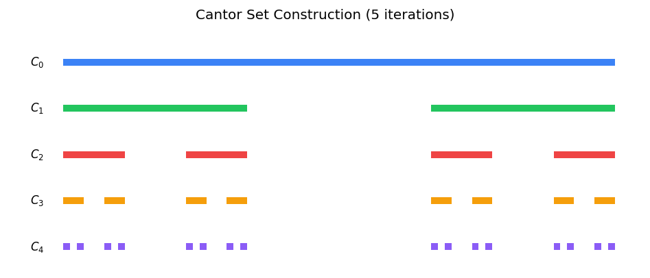
Cantor set construction: first 5 iterations

Definition 6.18 (Cantor Set). Let \(C_0 = [0,1]\). Construct \(C_{n+1}\) by removing the open middle third of each component interval of \(C_n\). The Cantor set is \(C = \bigcap_{n=0}^\infty C_n\).

The Cantor set is one of the most remarkable objects in mathematics — simultaneously “large” (uncountable, same cardinality as \(\mathbb{R}\)) and “small” (measure zero, nowhere dense). Understanding the Cantor set is essential preparation for measure theory and fractal geometry.

Proposition 6.18a (Ternary expansion characterization). A point \(x \in [0,1]\) belongs to the Cantor set \(C\) if and only if \(x\) has a ternary (base 3) expansion using only the digits 0 and 2: \[ C = \left\{x = \sum_{n=1}^\infty \frac{a_n}{3^n} : a_n \in \{0, 2\} \text{ for all } n\right\}. \]

Proof. At the first stage of the construction, \(C_1 = [0, 1/3] \cup [2/3, 1]\) consists of points whose first ternary digit is 0 or 2. Removing the middle third \((1/3, 2/3)\) eliminates exactly those points whose first ternary digit is 1 (being careful about endpoints, which have alternative representations). At the \(n\)-th stage, \(C_n\) consists of \(2^n\) intervals, and a point is in \(C_n\) if and only if its first \(n\) ternary digits are each 0 or 2. In the limit, \(C = \bigcap C_n\) consists of those points all of whose ternary digits are 0 or 2.

Properties of the Cantor set:

Closed (intersection of closed sets) and compact (closed and bounded in \(\mathbb{R}\)).
Totally disconnected: contains no interval. If \(a < b\) with \(a, b \in C\), then for large enough \(n\), the interval \((a,b)\) contains a removed middle-third interval, so \((a,b) \not\subseteq C\).
Perfect: every point is a limit point (\(C = C'\)). If \(x = \sum a_n/3^n \in C\), then changing the \(k\)-th digit from \(a_k\) to \(2 - a_k\) and keeping all other digits fixed gives a different point of \(C\) at distance \(\le 2/3^k \to 0\) from \(x\).
Nowhere dense: \((\overline{C})^\circ = \emptyset\), since \(C\) contains no interval.
Measure zero: the total length removed is \(1/3 + 2/9 + 4/27 + \cdots = \sum_{n=0}^\infty 2^n / 3^{n+1} = 1\). At stage \(n\), \(C_n\) consists of \(2^n\) intervals of total length \((2/3)^n \to 0\).
Uncountable: the map \(\phi: C \to \{0,1\}^{\mathbb{N}}\) given by \(\phi(\sum a_n/3^n) = (a_1/2, a_2/2, \ldots)\) is a bijection from \(C\) to the set of binary sequences. Since \(|\{0,1\}^{\mathbb{N}}| = 2^{\aleph_0} = \mathfrak{c}\), the Cantor set has the cardinality of the continuum, despite having measure zero.
Homeomorphic to \(\{0,1\}^{\mathbb{N}}\): the map \(\phi\) above is a homeomorphism when \(\{0,1\}^{\mathbb{N}}\) carries the product topology (equivalently, the metric \(d(s,t) = \sum 2^{-n} |s_n - t_n|\)). This is because the ternary expansion provides a dictionary between the Cantor set’s “left-right” branching structure and binary sequences.

Example 6.18b (The Cantor function --- "devil's staircase"). The Cantor function \(\varphi: [0,1] \to [0,1]\) is defined as follows. For \(x \in C\) with ternary expansion \(x = 0.a_1 a_2 \ldots\) (digits in \(\{0,2\}\)), set \(\varphi(x) = 0.b_1 b_2 \ldots\) in binary, where \(b_n = a_n/2\). On each removed interval \((a,b)\) in the complement of \(C\), extend \(\varphi\) by setting \(\varphi(x) = \varphi(a) = \varphi(b)\) (the function is constant on each gap). The Cantor function is:

Continuous and monotonically nondecreasing.
Differentiable almost everywhere, with \(\varphi'(x) = 0\) a.e. (on the complement of \(C\), which has full measure).
Surjective onto \([0,1]\): it maps the measure-zero set \(C\) onto all of \([0,1]\).
Not absolutely continuous: it increases from 0 to 1 but has derivative zero almost everywhere.

The Cantor function provides the classic example showing that a monotone continuous function with derivative zero a.e. need not be constant, illustrating the gap between the Riemann and Lebesgue theories of integration.

Theorem 6.19 (Space-filling curves). For any compact metric space \(X\), there exists a continuous surjection from the Cantor set \(C\) onto \(X\).

Proof. We construct a sequence of continuous functions \(f_k: C \to X\) converging uniformly to a continuous surjection.

Base case. Since \(X\) is compact, it has a finite \(1/2\)-net \(x_1^{(1)}, \ldots, x_{n_1}^{(1)}\) with \(n_1 \ge 2\). Partition \(C\) into \(n_1\) disjoint nonempty clopen subsets \(C_1^{(1)}, \ldots, C_{n_1}^{(1)}\) with \(\operatorname{diam}(C_i^{(1)}) \le 1/3\). (This is possible since \(C\) is perfect, compact, and totally disconnected.) Define \(f_1: C \to X\) by \(f_1|_{C_i^{(1)}} = x_i^{(1)}\). Being locally constant, \(f_1\) is continuous.

Inductive step. Suppose at stage \(k\) we have a \(2^{-k}\)-net \(\{x_i^{(k)}\}_{i=1}^{n_k}\), a partition of \(C\) into disjoint clopen sets \(\{C_i^{(k)}\}\) with \(\operatorname{diam}(C_i^{(k)}) \le 3^{-k}\), and a locally constant \(f_k: C \to X\) with \(f_k|_{C_i^{(k)}} = x_i^{(k)}\). For each \(i\), refine the ball \(B(x_i^{(k)}, 2^{-k})\) by choosing a \(2^{-(k+1)}\)-net of it, giving new points \(x_j^{(k+1,i)}\). Split each \(C_i^{(k)}\) into the same number of disjoint clopen subsets of diameter \(\le 3^{-(k+1)}\). Define \(f_{k+1}\) to be constant on each new piece, mapping to the corresponding net point.

Convergence. Since \(f_{k+1}(y) \in B(f_k(y), 2^{-k})\) for all \(y \in C\), we have \(\|f_{k+1} - f_k\|_\infty \le 2^{-k}\). Since \(\sum 2^{-k} < \infty\), the sequence \((f_k)\) is Cauchy in the complete space \(C(C, X)\) and converges uniformly to a continuous function \(f: C \to X\).

Surjectivity. Let \(x \in X\). At each stage \(k\), choose \(i_k\) with \(d(x, x_{i_k}^{(k)}) \le 2^{-k}\) and pick any \(y_k \in C_{i_k}^{(k)}\). The sequence of sets \(C_{i_1}^{(1)} \supseteq C_{i_2}^{(2)} \supseteq \cdots\) is nested, nonempty, and has diameters \(\to 0\). By Cantor’s Intersection Theorem, there exists \(y \in \bigcap_k C_{i_k}^{(k)}\). Then \(d(f(y), x) = \lim_k d(f_k(y), x) \le \lim_k 2^{-k} = 0\), so \(f(y) = x\).

Corollary 6.20. There exists a continuous surjection from \([0,1]\) onto \([0,1]^2\) (a space-filling curve). More generally, any compact metric space is a continuous image of \([0,1]\).

Proof. Given a continuous surjection \(f: C \to X\) from the Cantor set, extend it to \([0,1]\) as follows. Write \([0,1] \setminus C = \bigcup_{n=1}^\infty (a_n, b_n)\) as a disjoint union of open intervals (the "removed" intervals in the Cantor construction). Define \(\tilde{f}: [0,1] \to X\) by \(\tilde{f}(x) = f(x)\) for \(x \in C\), and on each gap \((a_n, b_n)\), set \(\tilde{f}(x) = \frac{b_n - x}{b_n - a_n} f(a_n) + \frac{x - a_n}{b_n - a_n} f(b_n)\) (linear interpolation, using convexity of \(X\) when applicable, or a geodesic in general). When \(X\) is a convex subset of a normed space, the extension is continuous and surjective. For the general case, one uses the fact that \(b_n - a_n \to 0\) and continuity of \(f\) on \(C\) to verify that \(\tilde{f}\) is continuous at each point of \(C\), hence everywhere.

Definition 6.20a (Peano Curve). A Peano curve (or space-filling curve) is a continuous surjection \(\gamma: [0,1] \to \mathbb{R}^n\) whose image has nonempty interior. The original construction by Peano (1890) mapped \([0,1]\) onto \([0,1]^2\), and Hilbert later gave a more geometric construction.

Theorem 6.21. Every nonempty, compact, perfect, totally disconnected metric space is homeomorphic to the Cantor set.

Proof. Let \(X\) be such a space and \(C\) the Cantor set. We build a homeomorphism by constructing approximating sequences of maps. Since \(X\) is compact and totally disconnected, the topology of \(X\) is generated by clopen (simultaneously closed and open) sets, and \(X\) can be partitioned into finitely many nonempty disjoint clopen subsets of arbitrarily small diameter. The perfectness of \(X\) (no isolated points) is essential: it guarantees that any nonempty clopen subset can be further subdivided, since a nonempty clopen subset of a perfect compact space is itself perfect and compact, hence contains at least two points, and can be split into smaller clopen pieces.

Construction. At the first stage, tile \(X\) with finitely many nonempty, disjoint, clopen sets \(X_1, \ldots, X_{n_1}\) of diameter at most \(1/2\), with \(n_1 \ge 2\). Partition \(C\) into the same number of disjoint clopen subsets \(C_1, \ldots, C_{n_1}\) with diameter at most \(1/3\) (this is always possible since the Cantor set is perfect and totally disconnected). Pick representative points \(x_i \in X_i\) and \(c_i \in C_i\), and define locally constant maps \(f_1: X \to C\) by \(f_1|_{X_i} = c_i\) and \(g_1: C \to X\) by \(g_1|_{C_i} = x_i\).

At the \(k\)-th stage, refine each \(X_i^{(k)}\) from the previous stage into finitely many disjoint clopen subsets of diameter at most \(2^{-k}\), and correspondingly refine each \(C_i^{(k)}\) into the same number of disjoint clopen subsets of diameter at most \(3^{-k}\). Define locally constant maps \(f_k: X \to C\) and \(g_k: C \to X\) by assigning each piece to a representative point.

Convergence. By construction, \(\|f_k - f_{k+1}\|_\infty \le 3^{-k}\) and \(\|g_k - g_{k+1}\|_\infty \le 2^{-k}\), so both \(\sum \|f_k - f_{k+1}\|_\infty\) and \(\sum \|g_k - g_{k+1}\|_\infty\) converge. Hence \((f_k)\) and \((g_k)\) are Cauchy in the complete spaces \(C(X, C)\) and \(C(C, X)\), and converge uniformly to continuous maps \(f: X \to C\) and \(g: C \to X\).

Inverse maps. At stage \(k\), \(\|g_k \circ f_k - \mathrm{id}_X\|_\infty \le \max_i \operatorname{diam}(X_i^{(k)}) \le 2^{-k} \to 0\) and similarly \(\|f_k \circ g_k - \mathrm{id}_C\|_\infty \le 3^{-k} \to 0\). Passing to limits, \(g \circ f = \mathrm{id}_X\) and \(f \circ g = \mathrm{id}_C\). Thus \(f\) and \(g\) are continuous bijections and inverses of each other, establishing the homeomorphism \(X \cong C\).

Remark. This theorem gives a topological characterization of the Cantor set: it is the unique (up to homeomorphism) nonempty compact metrizable space that is perfect and totally disconnected. The Cantor set thus serves as a "universal" totally disconnected compact space. Combined with Theorem 6.19 (every compact metric space is a continuous image of \(C\)), this makes the Cantor set a fundamental building block of compact metric spaces.

Chapter 7: Connectedness

While compactness captures “finiteness” of a space, connectedness captures the intuition that a space is “in one piece.” This chapter develops the basic theory of connected and path-connected spaces.

Connected spaces play a fundamental role in the intermediate value theorem, the classification of manifolds, and the theory of covering spaces. In metric spaces, the theory is somewhat simpler than in general topological spaces, but the key phenomena — the distinction between connectedness and path-connectedness, the existence of connected components — are already present.

7.1 Connected Sets

Definition 7.1. A metric space \(X\) is disconnected if there exist nonempty open sets \(U, V \subseteq X\) with \(U \cap V = \emptyset\) and \(X = U \cup V\). Such a pair \((U, V)\) is called a separation of \(X\). The space \(X\) is connected if it is not disconnected.

Equivalently, \(X\) is connected iff the only subsets that are both open and closed (clopen) are \(\emptyset\) and \(X\) itself.

Theorem 7.2. A subset \(A \subseteq \mathbb{R}\) is connected if and only if \(A\) is an interval (possibly unbounded or empty).

Proof. If \(A\) is not an interval, there exist \(a < c < b\) with \(a, b \in A\) but \(c \notin A\). Then \(U = A \cap (-\infty, c)\) and \(V = A \cap (c, \infty)\) form a separation. Conversely, suppose \(A\) is an interval and \(A = U \cup V\) is a separation. Choose \(a \in U\), \(b \in V\) with \(a < b\). Let \(c = \sup(U \cap [a,b])\). Since \(U\) is closed in \(A\), \(c \in U\); since \(U\) is open in \(A\), there exists \(\varepsilon > 0\) with \((c - \varepsilon, c + \varepsilon) \cap A \subseteq U\). But then \(c\) is not the supremum --- contradiction.

Theorem 7.3. The continuous image of a connected set is connected.

Proof. If \(f(X) = U \cup V\) is a separation, then \(X = f^{-1}(U) \cup f^{-1}(V)\) is a separation of \(X\).

Corollary 7.4 (Intermediate Value Theorem). If \(X\) is connected and \(f: X \to \mathbb{R}\) is continuous, then \(f(X)\) is an interval. In particular, if \(f(a) < 0 < f(b)\), there exists \(c\) between \(a\) and \(b\) with \(f(c) = 0\).

Example 7.4a (Applications of the IVT).

Existence of \(n\)-th roots: For any \(a > 0\) and \(n \ge 1\), the function \(f(x) = x^n - a\) is continuous on \([0, \max(1,a)]\) with \(f(0) < 0\) and \(f(\max(1,a)) \ge 0\). By the IVT, \(x^n = a\) has a positive root.
Every odd-degree polynomial has a real root: If \(p(x) = x^{2k+1} + a_{2k}x^{2k} + \cdots + a_0\), then \(p(x) \to +\infty\) as \(x \to +\infty\) and \(p(x) \to -\infty\) as \(x \to -\infty\). By the IVT, \(p\) has a zero.
The "ham sandwich theorem" in 1D: If \(f: [a,b] \to \mathbb{R}\) is continuous, there exists \(c \in [a,b]\) such that \(\int_a^c f = \int_c^b f\). Apply the IVT to \(g(c) = \int_a^c f - \int_c^b f\), which satisfies \(g(a) = -\int_a^b f\) and \(g(b) = \int_a^b f\).

Corollary 7.4b (Invariance of dimension for intervals). No continuous bijection exists between \([0,1]\) and \([0,1]^2\) (or more generally between \(\mathbb{R}^m\) and \(\mathbb{R}^n\) for \(m \ne n\)). In particular, \(\mathbb{R}\) and \(\mathbb{R}^2\) are not homeomorphic.

Proof for \(\mathbb{R}\) vs. \(\mathbb{R}^2\). Suppose \(f: \mathbb{R}^2 \to \mathbb{R}\) is a homeomorphism. Then \(f\) restricted to \(\mathbb{R}^2 \setminus \{p\}\) gives a homeomorphism to \(\mathbb{R} \setminus \{f(p)\}\). But \(\mathbb{R}^2 \setminus \{p\}\) is connected (any two points can be joined by a circular arc avoiding \(p\)), while \(\mathbb{R} \setminus \{f(p)\}\) is disconnected (it has two components). Connectedness is a topological invariant, so this is a contradiction.

Remark. This topological proof of non-homeomorphism is simple for \(\mathbb{R}\) vs. \(\mathbb{R}^2\), but the general case (\(\mathbb{R}^m \ncong \mathbb{R}^n\) for \(m \ne n\)) requires the more sophisticated tool of algebraic topology (homology groups). The key invariant is that \(\mathbb{R}^n \setminus \{0\}\) has the homotopy type of \(S^{n-1}\), and spheres of different dimensions are distinguished by their homology. The "invariance of domain" theorem (Brouwer, 1912) strengthens this: any continuous injection from an open subset of \(\mathbb{R}^n\) to \(\mathbb{R}^n\) is an open map.

Theorem 7.5. If \(A \subseteq X\) is connected and \(A \subseteq B \subseteq \overline{A}\), then \(B\) is connected. In particular, the closure of a connected set is connected.

Proof. If \(B = U \cup V\) is a separation, then since \(A\) is connected, \(A\) lies entirely in one of \(U\) or \(V\), say \(A \subseteq U\). Since \(U\) is closed in \(B\), \(\overline{A} \cap B \subseteq U\), but \(B \subseteq \overline{A}\), so \(B \subseteq U\), contradicting \(V \ne \emptyset\).

Theorem 7.6. If \(\{A_\alpha\}\) is a collection of connected subsets of \(X\) with \(\bigcap_\alpha A_\alpha \ne \emptyset\), then \(\bigcup_\alpha A_\alpha\) is connected.

Proof. Fix \(x_0 \in \bigcap_\alpha A_\alpha\). If \(\bigcup_\alpha A_\alpha = U \cup V\) is a separation, then \(x_0 \in U\) (say). For each \(\alpha\), \(A_\alpha\) is connected and \(x_0 \in A_\alpha \cap U\), so \(A_\alpha \subseteq U\). Thus \(\bigcup A_\alpha \subseteq U\), contradicting \(V \ne \emptyset\).

7.2 Path-Connectedness

Definition 7.7. A metric space \(X\) is path-connected if for every \(x, y \in X\), there exists a continuous map \(\gamma: [0,1] \to X\) with \(\gamma(0) = x\) and \(\gamma(1) = y\).

Theorem 7.8. Path-connected implies connected, but not conversely.

Proof. If \(X = U \cup V\) is a separation and \(\gamma: [0,1] \to X\) is a path from \(u \in U\) to \(v \in V\), then \(\gamma^{-1}(U) \cup \gamma^{-1}(V)\) separates \([0,1]\), contradicting the connectedness of \([0,1]\).

Example 7.9 (Topologist's sine curve). The set \(S = \{(x, \sin(1/x)) \mid x > 0\} \cup \{(0,y) \mid -1 \le y \le 1\}\) is connected but not path-connected. It is connected because it is the closure of the path-connected set \(\{(x, \sin(1/x)) : x > 0\}\) (Theorem 7.5). But no continuous path can cross from the segment \(\{0\} \times [-1,1]\) to the oscillating part.

Proof of non-path-connectedness. Suppose \(\gamma: [0,1] \to S\) is a continuous path with \(\gamma(0) = (0,0)\) and \(\gamma(1) = (1/\pi, 0)\). Write \(\gamma(t) = (\gamma_1(t), \gamma_2(t))\). Let \(t_0 = \sup\{t \in [0,1] : \gamma_1(t) = 0\}\). Then \(\gamma_1(t_0) = 0\) (by continuity) and \(\gamma_1(t) > 0\) for \(t > t_0\) sufficiently close to \(t_0\). For \(t > t_0\), the second coordinate satisfies \(\gamma_2(t) = \sin(1/\gamma_1(t))\). As \(t \to t_0^+\), we have \(\gamma_1(t) \to 0^+\), so \(1/\gamma_1(t) \to +\infty\), and \(\sin(1/\gamma_1(t))\) oscillates between \(-1\) and \(+1\). But \(\gamma_2(t)\) must converge to \(\gamma_2(t_0)\) by continuity --- a contradiction, since \(\sin(1/\gamma_1(t))\) does not converge.

Example 7.10. Convex subsets of \(\mathbb{R}^n\) are path-connected (hence connected): the straight-line segment \(\gamma(t) = (1-t)x + ty\) connects any two points.

Example 7.10a. Open connected subsets of \(\mathbb{R}^n\) are path-connected. Indeed, if \(U \subseteq \mathbb{R}^n\) is open and connected, fix \(a \in U\) and let \(V = \{x \in U : \exists \text{ path in } U \text{ from } a \text{ to } x\}\). Then \(V\) is open (if \(x \in V\), a small ball around \(x\) lies in \(U\) and can be connected to \(x\) by a straight line). Similarly, \(U \setminus V\) is open. Since \(U\) is connected and \(V \ne \emptyset\) (as \(a \in V\)), we have \(V = U\). This argument fails for general metric spaces, but it works for any locally path-connected space.

7.3 Connectedness of Products and Applications

Theorem 7.8a. The product \(X \times Y\) of connected metric spaces is connected.

Proof. Fix \((a,b) \in X \times Y\). For any \((x,y)\), the "L-shaped" set \(\{a\} \times Y \cup X \times \{y\}\) is connected (a union of two connected sets sharing the point \((a,y)\)) and contains both \((a,b)\) and \((x,y)\). Since \(X \times Y = \bigcup_{(x,y)} (\{a\} \times Y \cup X \times \{y\})\) and all these sets share \((a,b)\), the union is connected by Theorem 7.6.

Corollary 7.8b. \(\mathbb{R}^n\) is connected for all \(n \ge 1\). More generally, any path-connected space is connected, and any convex subset of a normed space is connected.

Theorem 7.8c (Fixed-point theorem for continuous maps on intervals). If \(f: [a,b] \to [a,b]\) is continuous, then \(f\) has a fixed point.

Proof. Apply the IVT to \(g(x) = f(x) - x\). We have \(g(a) = f(a) - a \ge 0\) and \(g(b) = f(b) - b \le 0\), so there exists \(c\) with \(g(c) = 0\), i.e., \(f(c) = c\).

7.4 Connected Components and Total Disconnectedness

Definition 7.11. The connected component of a point \(x \in X\) is the largest connected subset of \(X\) containing \(x\) (it exists as the union of all connected subsets containing \(x\)). Connected components are closed (since the closure of a connected set is connected) and partition \(X\). A space is totally disconnected if every connected component is a single point.

Definition 7.12 (Perfect set). A closed set \(A\) is perfect if it has no isolated points, i.e., every point of \(A\) is an accumulation point.

Theorem 7.13. Every perfect subset of \(\mathbb{R}\) is uncountable.

Proof. Let \(P\) be perfect. If \(P\) were countable, write \(P = \{p_1, p_2, \ldots\}\). The singletons \(\{p_n\}\) are nowhere dense (since \(P\) has no isolated points, every open interval meeting \(P\) contains another point of \(P\)). So \(P = \bigcup \{p_n\}\) is first category. But \(P\) is a complete metric space (closed in \(\mathbb{R}\)), so by the Baire Category Theorem, \(P\) cannot be first category --- contradiction.

Theorem 7.13a (Cantor--Bendixson). Every closed subset \(F\) of \(\mathbb{R}\) can be uniquely decomposed as \(F = P \cup C\) where \(P\) is perfect (possibly empty) and \(C\) is countable. Here \(P = F^{(\omega)} = \bigcap_{n=0}^\infty F^{(n)}\) where \(F^{(0)} = F\) and \(F^{(n+1)} = (F^{(n)})'\) (the derived set). In particular, every uncountable closed set contains a perfect subset, hence has cardinality \(\mathfrak{c}\).

Proposition 7.13b. Connected components are always closed. In compact spaces, if the space is totally disconnected, then the topology is generated by clopen sets.

Proof that components are closed. If \(C\) is the connected component of \(x\), then \(\overline{C}\) is connected (Theorem 7.5) and contains \(x\), so \(\overline{C} \subseteq C\) by maximality. Hence \(C = \overline{C}\) is closed.

Remark. Connected components are closed but not necessarily open. In the space \(\mathbb{Q}\), every connected component is a singleton \(\{q\}\), which is closed but not open (since \(\mathbb{Q}\) with the standard topology has no isolated points). If each connected component is open, the space is called locally connected. Manifolds, open subsets of \(\mathbb{R}^n\), and discrete spaces are locally connected; the Cantor set and the topologist's sine curve are not.

Example 7.14. The rationals \(\mathbb{Q}\), the Cantor set \(C\), and the p-adic integers \(\mathbb{Z}_p\) are all totally disconnected. For \(\mathbb{Q}\): if \(A \subseteq \mathbb{Q}\) contains two points \(a < b\), choose irrational \(c\) with \(a < c < b\); then \(A \cap (-\infty, c)\) and \(A \cap (c, \infty)\) disconnect \(A\).

Example 7.14a (Knaster--Kuratowski fan). This is an example of a connected space that becomes totally disconnected upon removing a single point. Let \(C\) be the Cantor set and \(p = (1/2, 1/2)\). For each \(c \in C\), let \(L(c)\) be the line segment from \((c,0)\) to \(p\). If \(c\) has a finite ternary expansion (i.e., \(c\) is an endpoint of a removed interval), let \(\chi_c = \{(x,y) \in L(c) : y \in \mathbb{Q}\}\); otherwise, let \(\chi_c = \{(x,y) \in L(c) : y \notin \mathbb{Q}\}\). Then \(F = \{p\} \cup \bigcup_{c \in C} \chi_c\) is connected, but \(F \setminus \{p\}\) is totally disconnected. This dramatic example shows that connectedness can be extremely fragile.

Chapter 8: The Baire Category Theorem

The Baire Category Theorem is one of the most powerful consequences of completeness. It provides a framework for proving that certain “nice” properties hold for “most” points or functions, even when constructing a single explicit example may be difficult.

The key idea is to classify subsets of a complete metric space as either “topologically small” (first category) or “topologically large” (second category/residual), and to show that complete metric spaces themselves are always second category.

8.1 Nowhere Dense Sets and Categories

Definition 8.1. A subset \(A\) of a metric space \(X\) is nowhere dense if \(\overline{A}\) has empty interior, i.e., \((\overline{A})^\circ = \emptyset\). Equivalently, for every nonempty open ball \(B\), there is a nonempty open ball \(C \subseteq B\) with \(C \cap A = \emptyset\).

Definition 8.2. A set \(A \subseteq X\) is first category (or meagre) if it is a countable union of nowhere dense sets. A set is second category if it is not first category. A set is residual (or comeagre) if its complement is first category.

First category sets are the “topologically small” sets, analogous to how measure-zero sets are “measure-theoretically small.” However, these notions are genuinely different: the Cantor set has measure zero but is not countable, and there exist sets of first category with positive measure.

Example 8.3. Every countable set in \(\mathbb{R}\) is first category (a countable union of singletons, each nowhere dense). In particular, \(\mathbb{Q}\) is first category in \(\mathbb{R}\). Every nowhere dense set is first category. Subsets of first category sets are first category. A countable union of first category sets is first category.

8.2 The Baire Category Theorem

Theorem 8.4 (Baire Category Theorem). Let \(X\) be a complete metric space. Then:

Every first category set in \(X\) has empty interior.
Every residual set in \(X\) is dense.
A countable union of closed sets with empty interiors has empty interior.
A countable intersection of dense open sets is dense.

Proof of (4). Let \(G_1, G_2, \ldots\) be dense open sets and \(B_0\) any nonempty open ball. Since \(G_1\) is dense, \(B_0 \cap G_1\) is nonempty and open. Choose a closed ball \(\overline{B}_1 \subseteq B_0 \cap G_1\) with radius \(r_1 < 1\). Since \(G_2\) is dense, \(B_1 \cap G_2\) is nonempty and open. Choose \(\overline{B}_2 \subseteq B_1 \cap G_2\) with \(r_2 < 1/2\). Continue to get nested closed balls \(\overline{B}_n \subseteq B_{n-1} \cap G_n\) with \(r_n < 1/n \to 0\). By Cantor's Intersection Theorem (in the complete space \(X\)), there exists \(x \in \bigcap \overline{B}_n \subseteq B_0 \cap \bigcap G_n\). So \(\bigcap G_n\) meets every open ball, hence is dense.

Proof of (1). Let \(A = \bigcup_{n=1}^\infty C_n\) where each \(C_n\) is nowhere dense. Then \(G_n = (\overline{C}_n)^c\) is open and dense. By (4), \(\bigcap G_n\) is dense, hence nonempty. But \(\bigcap G_n = (\bigcup \overline{C}_n)^c \subseteq A^c\), so \(A^c\) is dense, meaning \(A\) has empty interior.

Remark. Since \(\mathbb{Q}\) is first category and \(\mathbb{R}\) is complete, the BCT implies \(\mathbb{R} \setminus \mathbb{Q}\) is not first category (hence "topologically large"). Also, \(\mathbb{R}\) cannot be written as a countable union of nowhere dense sets, which distinguishes \(\mathbb{R}\) from \(\mathbb{Q}\) in a deep way. An immediate application: \(\mathbb{R}\) is uncountable, for if \(\mathbb{R} = \{r_1, r_2, \ldots\}\), then \(\mathbb{R} = \bigcup \{r_n\}\) would be first category, contradicting the BCT.

Remark (BCT for locally compact spaces). The Baire Category Theorem also holds for locally compact Hausdorff spaces (not necessarily complete metric spaces). This version is used in harmonic analysis and the theory of topological groups. The proof is essentially the same nested ball argument, using local compactness in place of completeness to guarantee the nested intersection is nonempty.

Corollary 8.4a (Banach's Category Theorem). In a complete metric space \(X\), the complement of a first category set is dense. Equivalently, \(X\) itself is not first category (second category in itself), and every nonempty open set is second category.

Proof. If \(A\) is first category, then \(A^c\) contains a residual set (the complement of the first category set), which is dense by the BCT. The second statement follows: if \(X = \bigcup A_n\) with each \(A_n\) nowhere dense, then \(X\) is first category, so \(X^c = \emptyset\) would be dense --- contradiction. For open sets: if the nonempty open set \(U\) were first category, then \(U = \bigcup C_n\) with \(C_n\) nowhere dense in \(X\). But \(U\) is open and nonempty, so \(A^\circ \ne \emptyset\) for \(A = U\), contradicting the BCT statement that first category sets have empty interior.

Example 8.4b (Application to algebraic numbers). The set \(\mathcal{A}\) of algebraic numbers is countable (there are countably many polynomials with integer coefficients, each with finitely many roots). So \(\mathcal{A}\) is first category in \(\mathbb{R}\). By Banach's category theorem, the set of transcendental numbers \(\mathbb{R} \setminus \mathcal{A}\) is residual, hence dense and uncountable. This gives a "topological" proof that transcendental numbers exist (and are typical) without constructing even a single one explicitly. Compare with Cantor's cardinality argument, which proves uncountability by a different route, and Liouville's construction, which gives explicit examples.

Remark (Category versus measure). First category (meagre) and measure zero are fundamentally different notions of "smallness," and neither implies the other:

The rationals \(\mathbb{Q}\) are first category in \(\mathbb{R}\) (a countable union of singletons) and have measure zero.
There exist dense open sets of arbitrarily small measure: for each \(\varepsilon > 0\), the set \(G_\varepsilon = \bigcup_{n=1}^\infty (q_n - \varepsilon/2^n, q_n + \varepsilon/2^n)\) (where \(\{q_n\}\) enumerates \(\mathbb{Q}\)) is open, dense, and has Lebesgue measure at most \(2\varepsilon\). Its complement \(\mathbb{R} \setminus G_\varepsilon\) is closed, nowhere dense, and has measure \(\ge 1 - 2\varepsilon\) on \([0,1]\). Taking a countable intersection \(\bigcap_{k=1}^\infty G_{1/k}\) gives a residual set of measure zero.
Conversely, the complement of such a set is first category but has full measure. So there exist sets that are "topologically large" (residual) but "measure-theoretically small" (measure zero), and vice versa.

The two notions capture genuinely different aspects of "largeness." The BCT concerns topological largeness; Lebesgue's theorem (PMATH 450) concerns measure-theoretic largeness. In ergodic theory and dynamical systems, understanding the interplay between these notions is a major theme.

Example 8.3a (Topological genericity). The BCT is often used to prove that a property holds for a "generic" (residual) set of objects:

Generic continuous functions are nowhere differentiable (Theorem 8.10).
Generic continuous functions are nowhere monotone: the set of \(f \in C[0,1]\) that are monotone on some interval is first category.
Generic orbits of irrational rotations are equidistributed: in the space of rotations of the circle, a residual set produces equidistributed orbits (Weyl's theorem).

These genericity results show that "pathological" objects (from the perspective of calculus) are actually typical in the topological sense.

8.3 \(G_\delta\) and \(F_\sigma\) Sets

Definition 8.5. In a metric (or topological) space \(X\):

A \(G_\delta\) set is a countable intersection of open sets.
An \(F_\sigma\) set is a countable union of closed sets.

Every closed set is \(G_\delta\) (in a metric space, \(A = \bigcap_{n=1}^\infty \{x : d(x,A) < 1/n\}\)) and every open set is \(F_\sigma\). The BCT implies that in a complete metric space, a dense \(G_\delta\) set is residual, and the intersection of countably many dense \(G_\delta\) sets is again dense \(G_\delta\).

Example 8.5a. The irrationals \(\mathbb{R} \setminus \mathbb{Q} = \bigcap_{q \in \mathbb{Q}} (\mathbb{R} \setminus \{q\})\) form a \(G_\delta\) subset of \(\mathbb{R}\) (a countable intersection of open sets). By contrast, \(\mathbb{Q} = \bigcup_{q \in \mathbb{Q}} \{q\}\) is \(F_\sigma\) (a countable union of closed sets). Neither is both \(G_\delta\) and \(F_\sigma\) simultaneously. Every open set is both \(G_\delta\) (trivially) and \(F_\sigma\) (write \(U = \bigcup \{K_n\}\) where \(K_n = \{x : d(x, U^c) \ge 1/n\}\)), and dually for closed sets. The Borel hierarchy \(\Sigma^0_1 = \text{open}\), \(\Pi^0_1 = \text{closed}\), \(\Sigma^0_2 = F_\sigma\), \(\Pi^0_2 = G_\delta\), etc., classifies sets by the complexity of their definition.

8.4 Oscillation and Continuity of Pointwise Limits

Definition 8.6 (Oscillation). For \(f: X \to Y\) and \(x \in X\), define the oscillation of \(f\) at \(x\): \[ \omega_f(x) = \inf_{\delta > 0} \sup_{y,z \in B(x,\delta)} d_Y(f(y), f(z)). \]

Then \(f\) is continuous at \(x\) if and only if \(\omega_f(x) = 0\).

Theorem 8.7. For any \(\varepsilon > 0\), the set \(\{x \in X : \omega_f(x) < \varepsilon\}\) is open. Therefore the set of points of continuity of \(f\) is a \(G_\delta\) set: \[ \{x : f \text{ is continuous at } x\} = \bigcap_{n=1}^\infty \{x : \omega_f(x) < 1/n\}. \]

Theorem 8.8. If \(f_n \in C[a,b]\) and \(f(x) = \lim_{n \to \infty} f_n(x)\) exists pointwise, then the set of points of continuity of \(f\) is a dense \(G_\delta\) set (hence residual).

Proof. By Theorem 8.7, the set of continuity points is a \(G_\delta\), so it suffices to show it is dense. Let \(A = \{x \in [a,b] : f \text{ is discontinuous at } x\}\). For each \(n \ge 1\), define \(A_n = \{x : \omega_f(x) \ge 1/n\}\). Since \(A = \bigcup_{n=1}^\infty A_n\), it suffices to show each \(A_n\) is nowhere dense.

Each \(A_n\) is closed by Theorem 8.7. Suppose for contradiction that some \(A_n\) contains an open interval \(I\). Fix \(\varepsilon = \frac{1}{3n}\). For each \(N \ge 1\), define

\[ E_N = \{x \in I : |f_i(x) - f_j(x)| \le \varepsilon \text{ for all } i, j \ge N\}. \]

Each \(E_N\) is closed (an intersection of closed sets). Since \(f_i(x) \to f(x)\) pointwise, for each \(x \in I\) the sequence \((f_i(x))\) is Cauchy, so \(x \in E_N\) for some \(N\). Thus \(I = \bigcup_{N=1}^\infty E_N\). By the Baire Category Theorem applied to the complete metric space \(I\), some \(E_{N_0}\) has nonempty interior, so there is an open sub-interval \(J \subseteq E_{N_0}\).

Fix \(x \in J\). By uniform continuity of \(f_{N_0}\) on \([a,b]\), there exists \(\delta > 0\) such that \(|x - y| < \delta \implies |f_{N_0}(x) - f_{N_0}(y)| < \varepsilon\). We may assume \((x - \delta, x + \delta) \subseteq J\). Then for \(|y - x| < \delta\):

\[ |f(x) - f(y)| \le |f(x) - f_{N_0}(x)| + |f_{N_0}(x) - f_{N_0}(y)| + |f_{N_0}(y) - f(y)| < \varepsilon + \varepsilon + \varepsilon = \frac{1}{n}, \]

where the first and third terms follow from \(|f(x) - f_{N_0}(x)| = \lim_{i \to \infty} |f_i(x) - f_{N_0}(x)| \le \varepsilon\) since \(x \in E_{N_0}\). This gives \(\omega_f(x) < 1/n\), so \(x \notin A_n\), contradicting \(J \subseteq I \subseteq A_n\).

This theorem shows that a pointwise limit of continuous functions, while not necessarily continuous everywhere, must be continuous on a “topologically large” set. The discontinuity set is meagre — it is contained in a countable union of nowhere dense sets.

Example 8.8a (Characterization of continuity sets). The converse question --- which \(G_\delta\) sets arise as continuity sets? --- has a complete answer: a subset \(D \subseteq \mathbb{R}\) is the set of continuity points of some function \(f: \mathbb{R} \to \mathbb{R}\) if and only if \(D\) is \(G_\delta\). The "only if" direction is Theorem 8.7. For the "if" direction, given a \(G_\delta\) set \(D = \bigcap G_n\), one constructs \(f\) by a careful modification of the characteristic function of \(\mathbb{Q} \cap D^c\). Notable consequences:

There exists a function continuous exactly on the irrationals (e.g., the Thomae function).
There does not exist a function continuous exactly on the rationals, because \(\mathbb{Q}\) is not \(G_\delta\) (Proposition 8.9a).
There exists a function continuous exactly on a given countable dense set \(D\) if and only if \(D\) is \(G_\delta\), which by the BCT requires \(D^c\) to be first category.

Remark. There is a precise characterization of which sets can be discontinuity sets of functions. A function \(f: \mathbb{R} \to \mathbb{R}\) is called Baire class 1 if it is the pointwise limit of continuous functions. The discontinuity set of a Baire class 1 function is always meagre \(F_\sigma\). Conversely, Lebesgue proved that any bounded function whose discontinuity set is meagre \(F_\sigma\) is Baire class 1. This means:

The characteristic function of the rationals \(\mathbf{1}_{\mathbb{Q}}\) is discontinuous everywhere, and since \(\mathbb{R}\) is not meagre (by the BCT), \(\mathbf{1}_{\mathbb{Q}}\) cannot be the pointwise limit of any sequence of continuous functions.
The Thomae function (Riemann function) \(f(p/q) = 1/q\), \(f(\text{irrational}) = 0\) is discontinuous exactly on \(\mathbb{Q}\), which is \(F_\sigma\) and meagre. Indeed, it is the pointwise limit of continuous functions (hence Baire class 1) and also Riemann integrable.

8.5 Application: The Uniform Boundedness Principle

The Baire Category Theorem has deep applications in functional analysis, even at the level of this course.

Theorem 8.9a (Uniform Boundedness Principle, baby version). Let \(X\) be a complete metric space and \(\{f_\alpha\}_{\alpha \in I}\) a family of continuous real-valued functions on \(X\) such that for every \(x \in X\), the set \(\{f_\alpha(x) : \alpha \in I\}\) is bounded. Then there exists a nonempty open ball \(B\) on which the family is uniformly bounded: \(\sup_\alpha \|f_\alpha\|_{C(B)} < \infty\).

Proof. For each \(n \ge 1\), define \(A_n = \{x \in X : |f_\alpha(x)| \le n \text{ for all } \alpha\} = \bigcap_{\alpha} f_\alpha^{-1}([-n, n])\). Each \(A_n\) is closed (intersection of closed sets). By hypothesis, every \(x\) lies in some \(A_n\), so \(X = \bigcup_{n=1}^\infty A_n\). By the Baire Category Theorem, some \(A_{n_0}\) has nonempty interior: there exists \(B(a, r) \subseteq A_{n_0}\). Then \(|f_\alpha(x)| \le n_0\) for all \(\alpha\) and all \(x \in B(a, r)\).

Remark. This result is the metric space precursor of the Banach--Steinhaus theorem (Uniform Boundedness Principle) in functional analysis: if a family of bounded linear operators is pointwise bounded, it is uniformly bounded. The proof strategy --- expressing the space as a countable union of closed sets and applying BCT to find one with nonempty interior --- is called the "Baire category method" and is one of the most important proof techniques in analysis. It produces existence results that are often impossible to obtain constructively.

8.5a Application: Smooth Functions with Polynomial Restrictions

Example 8.9. Let \(f \in C^\infty(\mathbb{R})\) and suppose that for every \(x \in \mathbb{R}\) there exists \(n_x \in \mathbb{N}\) with \(f^{(n_x)}(x) = 0\). Then there exists a nonempty open interval \((a,b)\) on which \(f\) is a polynomial. Indeed, let \(A_n = \{x : f^{(n)}(x) = 0\}\). Each \(A_n\) is closed (preimage of \(\{0\}\) under the continuous map \(f^{(n)}\)) and \(\bigcup A_n = \mathbb{R}\). By the BCT, some \(A_n\) has nonempty interior, so \(f^{(n)} = 0\) on an interval.

8.6 Application: \(\mathbb{Q}\) Is Not \(G_\delta\) in \(\mathbb{R}\)

Proposition 8.9a. The set \(\mathbb{Q}\) is \(F_\sigma\) (a countable union of closed singletons) but is not \(G_\delta\) in \(\mathbb{R}\).

Proof. Suppose \(\mathbb{Q} = \bigcap_{n=1}^\infty G_n\) with each \(G_n\) open. Since \(\mathbb{Q}\) is dense, each \(G_n\) is dense and open. Write \(\mathbb{Q} = \{q_1, q_2, \ldots\}\) and set \(V_n = \mathbb{R} \setminus \{q_n\}\), which is also dense and open. Then \[ \bigcap_{n=1}^\infty G_n \cap \bigcap_{n=1}^\infty V_n = \mathbb{Q} \cap (\mathbb{R} \setminus \mathbb{Q}) = \emptyset. \]

But by the BCT, a countable intersection of dense open sets in the complete space \(\mathbb{R}\) is dense, hence nonempty — contradiction.

This gives another proof that \(\mathbb{Q}\) is not complete: if it were, the BCT would apply to \(\mathbb{Q}\) itself, but \(\mathbb{Q} = \bigcup \{q_n\}\) is first category, so its interior (all of \(\mathbb{Q}\) if it had nonempty interior) would be empty — which it is. The more subtle point is that \(\mathbb{Q}\) cannot even be \(G_\delta\), which distinguishes it from the irrationals \(\mathbb{R} \setminus \mathbb{Q} = \bigcap_{n} (\mathbb{R} \setminus \{q_n\})\), which is \(G_\delta\).

8.7 Nowhere Differentiable Functions

One of the most striking applications of the Baire Category Theorem is showing that “most” continuous functions are nowhere differentiable.

Theorem 8.10. The set of continuous functions \(f \in C[0,1]\) that are differentiable at some point is a first category subset of \((C[0,1], d_\infty)\). Consequently, the nowhere differentiable functions form a residual (hence dense) set.

Proof (Sketch). Define \(A_{k,\ell} = \{f \in C[0,1] : \exists\, a \in [0,1],\, \forall\, x,\, 0 < |x-a| < 1/k \implies |\frac{f(x)-f(a)}{x-a}| \le \ell\}\). The set of functions differentiable somewhere is contained in \(\bigcup_{k,\ell} A_{k,\ell}\). Each \(A_{k,\ell}\) is closed (uniform limits preserve bounded difference quotients) and has empty interior (any function can be perturbed by a high-frequency sawtooth to destroy all bounded difference quotients). For the interior claim: given \(f \in A_{k,\ell}\) and \(\varepsilon > 0\), approximate \(f\) by a piecewise linear function \(h\) with \(\|h-f\|_\infty < \varepsilon/2\), then add \(\frac{\varepsilon}{2}\sin(Mx)\) with \(M\) large enough to produce slopes exceeding \(\ell\) at every point.

8.7 The Weierstrass Function

While the BCT gives an existential proof, Weierstrass gave an explicit example:

Example 8.11 (Weierstrass function). The function \[ f(x) = \sum_{k=1}^\infty 2^{-k} \cos(10^k \pi x) \]

is continuous everywhere (by the Weierstrass M-test, since \(\sum 2^{-k} < \infty\)) but differentiable nowhere.

Proof (Sketch). The function is 1-periodic. Fix \(x \in [0,1]\) and consider its decimal expansion \(x = 0.x_1x_2\ldots\). Define \(y_n = 0.x_1\ldots x_n\) (truncation) and \(z_n = y_n + 10^{-n}\). The key computation shows that for the \(n\)-th term, \(|f_n(y_n) - f_n(z_n)| = 2^{-n+1}\), while terms with \(k > n\) contribute zero and terms with \(k < n\) contribute at most \(\pi \cdot 2^{-n} \cdot 5^{-(n-k)}\). Summing, \(|f(y_n) - f(z_n)| > 2^{-n}\). By the pigeonhole principle, for some \(w_n \in \{y_n, z_n\}\), \(|f(w_n) - f(x)| > 2^{-n-1}\). Since \(|w_n - x| \le 10^{-n}\), the difference quotient \(|f(w_n) - f(x)|/|w_n - x| > 5^n/2 \to \infty\).

Remark (Historical significance and generalizations). Weierstrass's 1872 construction shocked the mathematical community, which had previously assumed continuous functions must be differentiable "almost everywhere" (a belief encouraged by the earlier work of Ampère). The general form of the Weierstrass function is \[ f(x) = \sum_{n=0}^\infty a^n \cos(b^n \pi x) \]

where \(0 < a < 1\), \(b\) is a positive odd integer, and \(ab > 1 + 3\pi/2\). Hardy (1916) proved the sharper result that nowhere-differentiability holds whenever \(ab \ge 1\), which is essentially optimal since \(ab < 1\) gives uniform convergence of the differentiated series by the Weierstrass M-test, yielding a differentiable function.

The Weierstrass function has Hölder exponent \(\alpha = -\log a/\log b\): it satisfies \(|f(x) - f(y)| \le C|x-y|^\alpha\) but not \(|f(x) - f(y)| \le C|x-y|^\beta\) for any \(\beta > \alpha\). This connects to fractal geometry: the graph of the Weierstrass function has Hausdorff dimension \(2 - \alpha\), which is strictly greater than 1, reflecting its rough, fractal-like nature.

Example 8.11a (Other nowhere differentiable functions). Several other explicit constructions are known:

Van der Waerden's function (1930): \(g(x) = \sum_{n=0}^\infty 10^{-n} \phi(10^n x)\) where \(\phi(x) = \min_{n \in \mathbb{Z}} |x - n|\) is the sawtooth function (distance to nearest integer). The proof of nowhere-differentiability is elementary: the \(n\)-th partial sum is piecewise linear with slopes \(\pm 1\), and the remaining terms contribute a controlled error.
Bolzano's function (~1830): Constructed decades before Weierstrass via a geometric process of progressively "zigzagging," though not published until much later. It demonstrates that pathological functions were being discovered even before the rigorous foundations of analysis were established.
Brownian motion: With probability 1, a sample path of standard Brownian motion is continuous and nowhere differentiable. This connects the analytic phenomenon to probability theory and provides a "random" construction complementing the explicit ones above.

Chapter 9: The Contraction Mapping Principle

The Contraction Mapping Principle (or Banach Fixed-Point Theorem) is a simple yet remarkably powerful consequence of completeness. It guarantees the existence and uniqueness of fixed points, and provides an explicit iterative algorithm for finding them.

9.1 Contraction Maps

Definition 9.1. Let \((X, d)\) be a metric space. A map \(T: X \to X\) is a contraction if there exists \(c \in [0,1)\) such that \(d(T(x), T(y)) \le c \cdot d(x,y)\) for all \(x, y \in X\). The constant \(c\) is called a contraction constant.

Every contraction is (uniformly) continuous, and strictly decreases distances between distinct points. The contraction constant \(c\) determines the rate of convergence: for \(c\) near 0 the convergence is fast, for \(c\) near 1 it is slow.

Example 9.1a (Contractions vs. non-expansive maps). The strict requirement \(c < 1\) is essential. The map \(T(x) = x + 1\) on \(\mathbb{R}\) has Lipschitz constant 1 and no fixed point. The map \(S(x) = x + 1/x\) on \([1, \infty)\) satisfies \(|S(x) - S(y)| = |1 - 1/(xy)| \cdot |x - y| < |x - y|\) for all \(x, y \ge 1\), but has no fixed point (since \(S(x) > x\) for all \(x \ge 1\)). The Lipschitz constant \(\sup_{x \ne y} |S(x) - S(y)|/|x - y| = \sup_{x,y \ge 1} |1 - 1/(xy)| = 1\), so \(S\) is not a contraction despite being "strictly non-expansive." This distinction between \(c < 1\) and \(c \le 1\) is one of the subtleties of the fixed-point theory.

9.2 The Banach Fixed-Point Theorem

Theorem 9.2 (Banach Fixed-Point Theorem). Let \((X, d)\) be a complete metric space and \(T: X \to X\) a contraction with constant \(c \in [0,1)\). Then:

\(T\) has a unique fixed point \(x^* \in X\).
For any \(x_0 \in X\), the iterates \(x_n = T^n(x_0)\) converge to \(x^*\).
The a priori error bound \(d(x_n, x^*) \le \frac{c^n}{1-c} d(x_0, T(x_0))\) holds.
The a posteriori error bound \(d(x_n, x^*) \le \frac{c}{1-c} d(x_{n-1}, x_n)\) holds.

Proof. Fix \(x_0 \in X\) and define \(x_n = T(x_{n-1})\). By induction, \(d(x_{n+1}, x_n) \le c^n d(x_1, x_0)\). For \(n < m\): \[ d(x_n, x_m) \le \sum_{i=n}^{m-1} d(x_{i+1}, x_i) \le c^n d(x_1, x_0) \sum_{j=0}^{m-n-1} c^j \le \frac{c^n}{1-c} d(x_1, x_0). \]

So \((x_n)\) is Cauchy, hence converges to some \(x^* \in X\). Since \(T\) is continuous, \(T(x^*) = T(\lim x_n) = \lim T(x_n) = \lim x_{n+1} = x^*\). For uniqueness: if \(T(a) = a\) and \(T(b) = b\), then \(d(a,b) = d(T(a), T(b)) \le c \cdot d(a,b)\) with \(c < 1\), forcing \(d(a,b) = 0\). The error bound follows by letting \(m \to \infty\) in the Cauchy estimate.

Remark (Practical significance of error bounds). The a priori bound \(d(x_n, x^*) \le \frac{c^n}{1-c} d(x_0, x_1)\) tells us in advance how many iterations are needed: to achieve accuracy \(\varepsilon\), we need \(n \ge \frac{\log(\varepsilon(1-c)/d(x_0,x_1))}{\log c}\), which is \(O(\log(1/\varepsilon))\) --- logarithmic in the desired precision. The a posteriori bound \(d(x_n, x^*) \le \frac{c}{1-c}d(x_{n-1}, x_n)\) is computable from the iterates and often sharper: once \(d(x_{n-1}, x_n)\) is observed to be small, the fixed point is nearby.

For example, with \(c = 1/2\) and \(d(x_0, x_1) = 1\): after \(n = 10\) iterations, \(d(x_{10}, x^*) \le 2^{-10}/(1 - 1/2) = 2^{-9} \approx 0.002\). After \(n = 20\): \(d(x_{20}, x^*) \le 2^{-19} \approx 10^{-6}\). The geometric convergence rate makes the theorem computationally practical.

Theorem 9.2a (Banach Fixed-Point for closed subsets). Let \(X\) be a complete metric space, \(A \subseteq X\) a closed subset, and \(T: A \to A\) a contraction. Then \(T\) has a unique fixed point in \(A\). Moreover, if \(T: X \to X\) is a contraction and \(T(A) \subseteq A\) for some closed subset \(A\), then the unique fixed point of \(T\) lies in \(A\).

Proof. Since \(A\) is closed in the complete space \(X\), the subspace \(A\) is complete (Theorem 5.3). Apply the Banach Fixed-Point Theorem to \(T: A \to A\). For the second statement: the fixed point \(x^*\) of \(T\) on \(X\) satisfies \(x^* = \lim T^n(x_0)\) for any \(x_0 \in A\). Since each \(T^n(x_0) \in A\) and \(A\) is closed, \(x^* \in A\).

9.3 Newton’s Method

Newton’s method is a prime application of the contraction mapping principle. The key insight is that the Newton operator \(T\) not only has a fixed point at the root, but has \(T'(x^*) = 0\), giving it “superlinear” contraction near \(x^*\).

Definition 9.3a (Quadratic Convergence). A sequence \(x_n \to x^*\) converges quadratically if there exists \(M > 0\) with \(|x_{n+1} - x^*| \le M|x_n - x^*|^2\) for all sufficiently large \(n\). Quadratic convergence is much faster than linear convergence (\(|x_{n+1} - x^*| \le c|x_n - x^*|\) with \(c < 1\)): if \(|x_n - x^*| \approx 10^{-k}\), then \(|x_{n+1} - x^*| \approx 10^{-2k}\), roughly doubling the number of correct digits per iteration.

Example 9.3 (Newton's method). To solve \(g(x) = 0\), define \(T(x) = x - g(x)/g'(x)\). If \(x^*\) is a simple root with \(g'(x^*) \ne 0\) and \(g\) is \(C^2\), then \[ T'(x) = 1 - \frac{(g'(x))^2 - g(x)g''(x)}{(g'(x))^2} = \frac{g(x)g''(x)}{(g'(x))^2}, \]

so \(T'(x^*) = 0\). By continuity, \(|T'(x)| \le 1/2\) on some interval \([x^* - R, x^* + R]\), making \(T\) a contraction. The convergence is quadratic: by Taylor expansion, \(|x_{n+1} - x^*| \le \frac{|g''(\xi_n)|}{2|g'(x_n)|} |x_n - x^*|^2\).

Example 9.3b (Computing \(\sqrt{a}\)). To find \(\sqrt{a}\), solve \(g(x) = x^2 - a = 0\). Newton's method gives \(T(x) = x - (x^2 - a)/(2x) = (x + a/x)/2\). Starting from \(x_0 = a\), the iterates converge quadratically to \(\sqrt{a}\). For \(a = 2\): \(x_0 = 2\), \(x_1 = 1.5\), \(x_2 = 1.41\overline{6}\), \(x_3 = 1.41421356\ldots\), matching \(\sqrt{2}\) to 8 digits in just 3 iterations. This is the Babylonian method, one of the oldest algorithms in mathematics.

Remark (The Implicit Function Theorem via contraction mapping). One of the most important applications of the contraction mapping principle is to the Implicit Function Theorem. Consider a continuously differentiable function \(F: \mathbb{R}^n \times \mathbb{R}^m \to \mathbb{R}^m\) with \(F(a, b) = 0\) and \(\det(D_y F(a, b)) \ne 0\), where \(D_y F\) denotes the partial Jacobian with respect to \(y\). The theorem asserts the existence of a \(C^1\) function \(g\) defined near \(a\) with \(g(a) = b\) and \(F(x, g(x)) = 0\).

The proof reduces to finding a fixed point. Define \(T_x(y) = y - [D_y F(a,b)]^{-1} F(x, y)\). Then \(F(x, y) = 0\) iff \(T_x(y) = y\). One computes \(D_y T_x(y) = I - [D_y F(a,b)]^{-1} D_y F(x,y)\). At \((a,b)\), this is \(I - I = 0\), so by continuity, \(\|D_y T_x\| < 1/2\) on a neighborhood of \((a,b)\). The Mean Value Inequality then shows \(T_x\) is a contraction in \(y\), and the Banach Fixed-Point Theorem gives a unique fixed point \(y = g(x)\). Smoothness of \(g\) follows from the smooth dependence of the fixed point on the parameter \(x\).

This argument generalizes to Banach spaces and is the standard approach to the Inverse Function Theorem as well: if \(F: U \to \mathbb{R}^n\) is \(C^1\) with \(\det(DF(a)) \ne 0\), local invertibility of \(F\) near \(a\) follows by applying the Implicit Function Theorem to \(G(x, y) = F(y) - x\).

9.4 Iterated Function Systems and Fractals

A beautiful application of the Contraction Mapping Principle is to iterated function systems (IFS).

Definition 9.5 (Hausdorff Metric on Compact Subsets). Let \((X,d)\) be a complete metric space. The collection \(\mathcal{H}(X) = \{K \subseteq X : K \text{ is nonempty and compact}\}\) is a metric space under the Hausdorff metric \(d_H(A,B) = \max\{\sup_{a \in A} d(a,B),\, \sup_{b \in B} d(b,A)\}\). When \(X\) is complete, \(\mathcal{H}(X)\) is complete.

Lemma 9.6. For compact sets \(A_1, \ldots, A_n\) and \(B_1, \ldots, B_n\) in a metric space, \[ d_H\left(\bigcup_{i=1}^n A_i,\, \bigcup_{i=1}^n B_i\right) \le \max_{1 \le i \le n} d_H(A_i, B_i). \]

Proof. Let \(r = \max_i d_H(A_i, B_i)\). Then \(A_i \subseteq E_r(B_i)\) (the \(r\)-neighborhood of \(B_i\)), so \(\bigcup A_i \subseteq E_r(\bigcup B_i)\). By symmetry, \(\bigcup B_i \subseteq E_r(\bigcup A_i)\), giving \(d_H(\bigcup A_i, \bigcup B_i) \le r\).

Theorem 9.7 (IFS Attractor). Let \((X,d)\) be a complete metric space and \(T_1, \ldots, T_k: X \to X\) contractions with constants \(c_1, \ldots, c_k < 1\). Define \(\mathcal{T}: \mathcal{H}(X) \to \mathcal{H}(X)\) by \(\mathcal{T}(A) = T_1(A) \cup \cdots \cup T_k(A)\). Then:

Each \(T_i\) is a contraction on \(\mathcal{H}(X)\): \(d_H(T_i(A), T_i(B)) \le c_i \cdot d_H(A,B)\).
\(\mathcal{T}\) is a contraction with constant \(c = \max_i c_i < 1\).
\(\mathcal{T}\) has a unique fixed point \(K^* \in \mathcal{H}(X)\) --- the attractor of the IFS --- satisfying \(K^* = T_1(K^*) \cup \cdots \cup T_k(K^*)\).

Proof. For (1): let \(a \in A\). Choose \(b_a \in B\) with \(d(a, b_a) \le d_H(A,B)\). Then \(d(T_i(a), T_i(b_a)) \le c_i d(a, b_a) \le c_i d_H(A,B)\), so \(T_i(A) \subseteq E_{c_i d_H(A,B)}(T_i(B))\). By symmetry, \(d_H(T_i(A), T_i(B)) \le c_i d_H(A,B)\). For (2): by Lemma 9.6 and (1), \(d_H(\mathcal{T}(A), \mathcal{T}(B)) \le \max_i c_i \cdot d_H(A,B)\). Part (3) follows from the Banach Fixed-Point Theorem applied to the complete space \(\mathcal{H}(X)\).

The attractor can be approximated starting from any compact set \(K_0\): the iterates \(K_n = \mathcal{T}^n(K_0)\) converge to \(K^*\) in the Hausdorff metric. The Banach Fixed-Point Theorem gives the error bound \(d_H(K_n, K^*) \le \frac{c^n}{1-c} d_H(K_0, \mathcal{T}(K_0))\). In practice, starting from any simple compact set (a point, a line segment, or a filled triangle) and repeatedly applying \(\mathcal{T}\) produces increasingly detailed approximations of the fractal attractor.

Remark (The "address" system for IFS attractors). Each point \(x^* \in K^*\) in the attractor of an IFS with \(k\) maps can be encoded by an infinite sequence \((\omega_1, \omega_2, \ldots)\) with \(\omega_i \in \{1, \ldots, k\}\), called an address or symbolic itinerary. The point is recovered as \(x^* = \lim_{n \to \infty} T_{\omega_1} \circ T_{\omega_2} \circ \cdots \circ T_{\omega_n}(x_0)\) for any starting point \(x_0\). This encoding establishes a continuous surjection from the sequence space \(\{1, \ldots, k\}^{\mathbb{N}}\) (a Cantor-like space) onto the attractor, connecting the theory of iterated function systems to symbolic dynamics.

Example 9.8. The Sierpinski triangle arises from three affine contractions on \(\mathbb{R}^2\), each shrinking by factor \(1/2\) toward a vertex of an equilateral triangle: \(T_0(x) = x/2\), \(T_1(x) = x/2 + (2,0)/2\), \(T_2(x) = x/2 + (1,\sqrt{3})/2\). Starting from any compact set (e.g., the solid triangle), the iterates converge to the Sierpinski triangle. The Cantor set arises from \(T_1(x) = x/3\) and \(T_2(x) = x/3 + 2/3\) on \([0,1]\). The Koch snowflake boundary arises from four contractions of ratio \(1/3\).

Example 9.9 (Local contraction principle). If \(T \in C^1([a,b], [a,b])\) with \(T(x^*) = x^*\) and \(|T'(x^*)| < 1\), then by continuity there exists \(\delta > 0\) such that \(\sup_{|x - x^*| \le \delta} |T'(x)| = c < 1\). By the Mean Value Theorem, \(T\) is a contraction on \(\overline{B}(x^*, \delta)\) with constant \(c\). This gives local convergence of iterates near fixed points of smooth maps and is the theoretical basis for many numerical algorithms.

Remark (Hausdorff dimension of IFS attractors). For an IFS \(\{T_1, \ldots, T_k\}\) where each \(T_i\) is a similarity (not just a contraction) with ratio \(r_i\), and the maps satisfy the open set condition (there exists a nonempty bounded open set \(V\) with \(\bigcup T_i(V) \subseteq V\) and the images pairwise disjoint), the Hausdorff dimension of the attractor \(K^*\) is the unique \(s \ge 0\) satisfying \[ \sum_{i=1}^k r_i^s = 1 \]

(the Moran equation). This is sometimes called the similarity dimension. For example:

The Cantor set has \(k = 2\), \(r_1 = r_2 = 1/3\), so \(2 \cdot (1/3)^s = 1\), giving \(s = \log 2 / \log 3 \approx 0.631\).
The Sierpinski triangle has \(k = 3\), \(r_i = 1/2\), so \(3 \cdot (1/2)^s = 1\), giving \(s = \log 3 / \log 2 \approx 1.585\).
The Koch curve has \(k = 4\), \(r_i = 1/3\), giving \(s = \log 4 / \log 3 \approx 1.262\).

The fact that these dimensions are non-integer is what makes fractals "fractional-dimensional" --- the original motivation for Mandelbrot's term "fractal."

Theorem 9.9a (Collage Theorem). If \(K_0 \in \mathcal{H}(X)\) satisfies \(d_H(K_0, \mathcal{T}(K_0)) \le \varepsilon\), then the attractor satisfies \(d_H(K_0, K^*) \le \varepsilon/(1-c)\), where \(c = \max_i c_i\) is the contraction constant. In other words, if a set approximately satisfies the self-similarity equation, it is close to the true fractal.

Proof. This is a direct consequence of the Banach Fixed-Point error estimate. Since \(\mathcal{T}\) is a contraction with constant \(c\) on the complete space \(\mathcal{H}(X)\), and \(K^* = \mathcal{T}(K^*)\): \[ d_H(K_0, K^*) \le \frac{d_H(K_0, \mathcal{T}(K_0))}{1 - c} \le \frac{\varepsilon}{1 - c}. \]

Remark. The Collage Theorem is the theoretical basis for fractal image compression: to encode an image \(K_0\), find an IFS whose attractor \(K^*\) is close to \(K_0\). The IFS (a small collection of affine maps) serves as a highly compressed representation. The collage theorem guarantees that if \(\mathcal{T}(K_0) \approx K_0\), then \(K^* \approx K_0\). This technique was developed by Barnsley and others in the 1990s.

Chapter 10: Metric Completion and p-adic Numbers

Every metric space, no matter how incomplete, can be “filled in” to create a complete space. This chapter develops the theory of metric completion, applies it to construct the p-adic numbers, and shows how the real numbers themselves can be constructed as the completion of the rationals.

10.1 Existence of the Metric Completion

The central result of this section asserts that every metric space can be “completed” by adding the limits of Cauchy sequences that are “missing.” The construction is analogous to how \(\mathbb{R}\) is obtained from \(\mathbb{Q}\) by filling in the irrational numbers.

Theorem 10.1 (Metric Completion). Every metric space \((X,d)\) has a completion: a complete metric space \((\hat{X}, \hat{d})\) together with an isometric embedding \(J: X \to \hat{X}\) such that \(J(X)\) is dense in \(\hat{X}\).

Proof. Fix \(a \in X\). For each \(x \in X\), define \(f_x: X \to \mathbb{R}\) by \(f_x(t) = d(t,x) - d(t,a)\). By the triangle inequality, \(|f_x(t)| \le d(x,a)\), so \(f_x\) is bounded. Also \(f_x\) is Lipschitz: \(|f_x(s) - f_x(t)| \le 2d(s,t)\). The map \(F: X \to C_b(X)\) defined by \(F(x) = f_x\) is an isometry: \[ \|f_x - f_y\|_\infty = \sup_{t \in X} |d(t,x) - d(t,y)| = d(x,y), \]

where the supremum is attained at \(t = y\). Since \(C_b(X)\) is complete, the closure \(\overline{F(X)}\) is a complete metric space containing \(F(X) \cong X\) as a dense subset.

Remark. An alternative construction uses equivalence classes of Cauchy sequences: define \(\hat{X}\) to be the set of all Cauchy sequences in \(X\), modulo the equivalence \((x_n) \sim (y_n)\) when \(\lim d(x_n, y_n) = 0\). The metric \(\hat{d}([(x_n)], [(y_n)]) = \lim d(x_n, y_n)\) makes \(\hat{X}\) complete, and the map \(x \mapsto [(x, x, x, \ldots)]\) is an isometric embedding with dense image.

Example 10.1a (Completions of familiar spaces). The completion construction unifies several important constructions in mathematics:

The completion of \((\mathbb{Q}, |\cdot|)\) is \(\mathbb{R}\) (by definition/construction).
The completion of \((\mathbb{Q}, |\cdot|_p)\) is the p-adic numbers \(\mathbb{Q}_p\) (Section 10.3).
The completion of \((C[a,b], \|\cdot\|_1)\) is the Lebesgue space \(L^1[a,b]\) (developed in PMATH 450).
The completion of \((C[a,b], \|\cdot\|_2)\) is the Hilbert space \(L^2[a,b]\), fundamental to quantum mechanics and Fourier analysis.
The completion of the rational polynomials under the p-adic valuation gives the ring of formal power series, an important tool in algebraic geometry.

In each case, the incomplete space is dense in its completion, and the completion inherits the algebraic structure (addition, multiplication) from the original space by uniform continuity of the operations.

10.2 Uniqueness of the Metric Completion

Having shown that completions exist, we now show they are unique up to isometry. This is analogous to the uniqueness of the real numbers as a complete ordered field. The proof uses the extension theorem for uniformly continuous maps, which is itself a consequence of completeness.

Theorem 10.2 (Uniqueness). If \(Y\) and \(Z\) are both complete metric spaces containing \(X\) as a dense subset (via isometric embeddings), then there is a unique isometry \(F: Y \to Z\) with \(F(x) = x\) for all \(x \in X\).

Proof. For \(a \in Y\), choose \((x_n)\) in \(X\) with \(x_n \to a\) in \(Y\). Then \((x_n)\) is Cauchy in \(X\), hence Cauchy in \(Z\), hence converges in \(Z\). Define \(F(a) = \lim x_n\) in \(Z\). This is well-defined: if \((y_n)\) also converges to \(a\) in \(Y\), then \(d_Z(\lim x_n, \lim y_n) = \lim d_X(x_n, y_n) = \lim d_Y(x_n, y_n) = 0\). The map \(F\) preserves distances since \(d_Z(F(a), F(b)) = \lim d_X(x_n, y_n) = \lim d_Y(x_n, y_n) = d_Y(a, b)\).

Theorem 10.3 (Extension of uniformly continuous maps). If \(X\) is dense in \(\hat{X}\) and \(f: X \to Y\) is uniformly continuous with \(Y\) complete, then \(f\) extends uniquely to a uniformly continuous map \(\hat{f}: \hat{X} \to Y\).

Proof. Definition of \(\hat{f}\): For \(a \in \hat{X}\), choose \((x_n)\) in \(X\) with \(x_n \to a\). Since \(f\) is uniformly continuous and \((x_n)\) is Cauchy, \((f(x_n))\) is Cauchy in \(Y\): given \(\varepsilon > 0\), choose \(\delta > 0\) from uniform continuity, then \(N\) with \(d(x_n, x_m) < \delta\) for \(n, m \ge N\), giving \(d(f(x_n), f(x_m)) < \varepsilon\). Since \(Y\) is complete, define \(\hat{f}(a) = \lim f(x_n)\).

Well-definedness: If \((y_n)\) also converges to \(a\), then \(d(x_n, y_n) \to 0\), so \(d(f(x_n), f(y_n)) \to 0\) by uniform continuity, giving \(\lim f(x_n) = \lim f(y_n)\).

Uniform continuity of \(\hat{f}\): Given \(\varepsilon > 0\), choose \(\delta > 0\) with \(d(x,y) < \delta \implies d(f(x), f(y)) < \varepsilon\) for \(x, y \in X\). If \(d(a,b) < \delta\) in \(\hat{X}\), choose \(x_n \to a\) and \(y_n \to b\) in \(X\). Then \(d(x_n, y_n) \to d(a,b) < \delta\), so for large \(n\), \(d(f(x_n), f(y_n)) < \varepsilon\). Taking limits: \(d(\hat{f}(a), \hat{f}(b)) \le \varepsilon\).

Uniqueness: If \(\hat{g}\) is another continuous extension, then \(\hat{f}\) and \(\hat{g}\) agree on the dense set \(X\), and the set \(\{a \in \hat{X} : \hat{f}(a) = \hat{g}(a)\}\) is closed (preimage of the diagonal under the continuous map \(a \mapsto (\hat{f}(a), \hat{g}(a))\)). A closed set containing a dense subset equals the whole space, so \(\hat{f} = \hat{g}\).

Remark. This extension theorem is the metric space analogue of the principle that "a continuous function is determined by its values on a dense set." It fails without uniform continuity: the function \(f(x) = \sin(1/x)\) is continuous on \((0,1]\) but has no continuous extension to \([0,1]\). It also fails without completeness of the target: the identity map \(\mathrm{id}: \mathbb{Q} \to \mathbb{Q}\) is uniformly continuous, but there is no continuous map from \(\mathbb{R}\) to \(\mathbb{Q}\) that extends it (any such map would have connected image, but the only connected subsets of \(\mathbb{Q}\) are singletons and the empty set). The theorem has deep consequences: it shows that the metric completion is functorial, and it is the key ingredient in proving uniqueness of the completion.

10.3 The p-adic Numbers

The p-adic numbers provide the most important example of metric completion beyond the construction of \(\mathbb{R}\). They were introduced by Hensel in 1897 and are fundamental in number theory and algebraic geometry.

Definition 10.4. Fix a prime \(p\). The p-adic integers \(\mathbb{Z}_p\) is the completion of \(\mathbb{Z}\) with respect to the p-adic metric \(d_p\). The p-adic numbers \(\mathbb{Q}_p\) is the completion of \(\mathbb{Q}\) with respect to \(d_p\). The p-adic norm of a nonzero rational \(x = p^a(r/s)\) with \(\gcd(r,p) = \gcd(s,p) = 1\) is \(|x|_p = p^{-a}\), and \(|0|_p = 0\).

Proposition 10.5 (Field structure of \(\mathbb{Q}_p\)). The arithmetic operations on \(\mathbb{Q}\) extend continuously to \(\mathbb{Q}_p\). Specifically, if \((x_n), (y_n)\) are Cauchy sequences in \((\mathbb{Q}, d_p)\) with limits \(x, y \in \mathbb{Q}_p\), then:

\(x + y = \lim(x_n + y_n)\) and \(xy = \lim(x_n y_n)\) are well-defined.
\(\|xy\|_p = \|x\|_p \|y\|_p\) (multiplicativity).
\(\|x + y\|_p \le \max\{\|x\|_p, \|y\|_p\}\) (ultrametric inequality).

Moreover, \(\mathbb{Q}_p\) is a topologically complete field containing \(\mathbb{Q}\) as a dense subfield.

Proof (Sketch). For addition: \(\|(x_n + y_n) - (x_m + y_m)\|_p \le \max\{\|x_n - x_m\|_p, \|y_n - y_m\|_p\} \to 0\), so the sum sequence is Cauchy. For multiplication: \(\|x_n y_n - x_m y_m\|_p = \|(x_n - x_m)y_n + x_m(y_n - y_m)\|_p\), and since \(\|x_n\|_p, \|y_n\|_p\) are eventually constant (for nonzero limits) or bounded, this tends to 0. For inverses: if \(x \ne 0\), then \(\|x_n\|_p = \|x\|_p\) for large \(n\), so \(\|1/x_n - 1/x_m\|_p = \|x_m - x_n\|_p / (\|x_n\|_p \|x_m\|_p) = \|x_m - x_n\|_p / \|x\|_p^2 \to 0\).

Proposition 10.6 (p-adic expansion). Every p-adic integer has a unique representation as a convergent series \(x = \sum_{i=0}^\infty \alpha_i p^i\) where \(\alpha_i \in \{0, 1, \ldots, p-1\}\). More generally, every nonzero p-adic number can be written \(x = \sum_{i=-k}^\infty \alpha_i p^i\) for some integer \(k\).

Proof. For \(x \in \mathbb{Z}_p\), we construct the digits inductively. For \(n = 0\): since \(\{0, 1, \ldots, p-1\}\) is a \(p^{-1}\)-net for \(\mathbb{Z}_p\), there is a unique \(\alpha_0 \in \{0, \ldots, p-1\}\) with \(\|x - \alpha_0\|_p \le 1/p\). Uniqueness holds because if \(\alpha_0 \ne \beta_0\), then \(\|\alpha_0 - \beta_0\|_p = 1\) (since \(p \nmid (\alpha_0 - \beta_0)\)), contradicting \(\|x - \alpha_0\|_p, \|x - \beta_0\|_p \le 1/p\) via the ultrametric inequality. Inductively, having chosen \(\alpha_0, \ldots, \alpha_{n-1}\), the element \(y = p^{-n}(x - \sum_{i=0}^{n-1} \alpha_i p^i)\) satisfies \(\|y\|_p \le 1\), and we choose \(\alpha_n\) as the unique digit with \(\|y - \alpha_n\|_p \le 1/p\). The partial sums \(S_n = \sum_{i=0}^n \alpha_i p^i\) satisfy \(\|x - S_n\|_p \le p^{-n-1} \to 0\).

Example 10.7 (p-adic expansion of \(-1\)). In \(\mathbb{Z}_p\), the element \(-1\) has the expansion \(-1 = (p-1) + (p-1)p + (p-1)p^2 + \cdots\), since the partial sums \(S_n = p^n - 1\) satisfy \(|S_n - (-1)|_p = |p^n|_p = p^{-n} \to 0\). This illustrates the radically different nature of p-adic convergence: the "infinite" sum of positive terms yields \(-1\).

Proposition 10.8. \(\mathbb{Z}_p\) is compact.

Proof. \(\mathbb{Z}_p\) is complete (closed in the complete space \(\mathbb{Q}_p\)) and totally bounded: the set \(\{0, 1, \ldots, p^n - 1\}\) is a \(p^{-n}\)-net for \(\mathbb{Z}_p\). Hence \(\mathbb{Z}_p\) is compact by Theorem 6.7.

The p-adic numbers satisfy the ultrametric inequality \(d_p(x,z) \le \max\{d_p(x,y), d_p(y,z)\}\), which gives them a very different geometry from \(\mathbb{R}\):

Every triangle is isosceles: if \(d_p(x,y) \ne d_p(y,z)\), then \(d_p(x,z) = \max\{d_p(x,y), d_p(y,z)\}\). (In an ultrametric, the two largest sides of any triangle are equal.)
Every point in a ball is a center: if \(b \in B(a,r)\), then \(B(a,r) = B(b,r)\). Proof: if \(x \in B(a,r)\), then \(d_p(x,b) \le \max\{d_p(x,a), d_p(a,b)\} < r\), so \(x \in B(b,r)\). By symmetry, \(B(a,r) = B(b,r)\).
Two balls are either disjoint or one contains the other. If \(B(a,r) \cap B(b,s) \ne \emptyset\) with \(r \le s\), pick \(c\) in the intersection. Then \(B(a,r) = B(c,r) \subseteq B(c,s) = B(b,s)\).
Balls are clopen: the open ball \(B(a,r)\) is also closed, and the closed ball \(\overline{B}(a,r)\) is also open. This is because the p-adic norm takes only the discrete values \(\{0, p^{-n} : n \in \mathbb{Z}\}\), so there is always a "gap" between the boundary and the exterior.
\(\mathbb{Z}_p\) is totally disconnected, compact, and perfect.

Since \(\mathbb{Z}_p\) is compact, perfect, and totally disconnected, by Theorem 6.21 it is homeomorphic to the Cantor set. This gives a concrete realization of an abstract topological characterization.

Example 10.8a (Arithmetic in \(\mathbb{Z}_p\)). The p-adic integers support surprising arithmetic. In \(\mathbb{Z}_5\):

The equation \(x^2 = -1\) has a solution! Starting with \(x_0 = 2\) (since \(2^2 = 4 \equiv -1 \pmod{5}\)), Newton's method in \(\mathbb{Z}_5\) produces a Cauchy sequence converging to a square root of \(-1\). Explicitly, \(i_5 = 2 + 1 \cdot 5 + 2 \cdot 5^2 + 1 \cdot 5^3 + \cdots\) satisfies \(i_5^2 = -1\) in \(\mathbb{Z}_5\).
The equation \(x^2 = 2\) has no solution in \(\mathbb{Z}_5\), since 2 is not a quadratic residue mod 5.

More generally, Hensel's lemma provides a p-adic analogue of Newton's method: if a polynomial equation has a "simple" solution modulo \(p\), it lifts to a solution in \(\mathbb{Z}_p\). This is the starting point for a rich interplay between algebra and analysis in number theory.

Example 10.8b (The p-adic integers as inverse limit). The quotient maps \(\pi_n: \mathbb{Z}_p \to \mathbb{Z}/p^n\mathbb{Z}\) sending \(x = \sum \alpha_i p^i\) to \(\sum_{i=0}^{n-1} \alpha_i p^i \pmod{p^n}\) satisfy \(\pi_{n+1} \circ \pi_n = \pi_n\). This exhibits \(\mathbb{Z}_p\) as the inverse limit (or projective limit) of the finite rings \(\mathbb{Z}/p^n\mathbb{Z}\): \[ \mathbb{Z}_p = \varprojlim \mathbb{Z}/p^n\mathbb{Z} = \left\{(a_n)_{n \ge 1} \in \prod_{n \ge 1} \mathbb{Z}/p^n\mathbb{Z} : a_{n+1} \equiv a_n \pmod{p^n}\right\}. \]

This algebraic perspective reveals \(\mathbb{Z}_p\) as the completion of \(\mathbb{Z}\) in the p-adic metric, and explains why the topology (a product of discrete finite spaces) is compact, totally disconnected, and metrizable.

10.4 Ordered Fields and the Construction of \(\mathbb{R}\)

The real numbers can be characterized abstractly as the unique complete ordered field. To make this precise, we need the language of ordered fields.

Definition 10.9 (Ordered Field). An ordered field is a field \(F\) equipped with a subset \(P \subseteq F\) (the "positive" elements) satisfying:

\(F = (-P) \cup \{0\} \cup P\) (disjoint union), where \(-P = \{-x : x \in P\}\).
\(P + P \subseteq P\) and \(P \cdot P \subseteq P\).

The ordering is defined by \(x < y\) iff \(y - x \in P\).

Definition 10.10 (Least Upper Bound Property). An ordered field has the least upper bound property (LUBP) if every nonempty subset that is bounded above has a least upper bound (supremum). An ordered field is Archimedean if for every \(x > 0\), there exists \(n \in \mathbb{N}\) with \(1/n < x\).

Proposition 10.11. Let \(F\) be an ordered field.

\(\mathbb{Q}\) embeds into \(F\) as an ordered subfield (since \(0 < 1 < 1 + 1 < \cdots\), so \(\mathbb{Z} \subseteq F\), hence \(\mathbb{Q} \subseteq F\)). In particular, \(F\) has characteristic 0.
The LUBP implies completeness (every Cauchy sequence converges).
The LUBP implies the Archimedean property.
The Archimedean property implies \(\mathbb{Q}\) is dense in \(F\): if \(x < y\), there exists \(r \in \mathbb{Q}\) with \(x < r < y\).

Proof of (3). Suppose \(F\) has the LUBP but is not Archimedean. Then \(J = \{x > 0 : nx < 1 \text{ for all } n \ge 1\} \ne \emptyset\). The set \(J\) is bounded above by 1, so \(y = \sup J\) exists. For any \(x_0 \in J\), we have \(x_0 + x_0 \in J\) (since \(n(2x_0) = 2nx_0 < 2 \cdot 1\) does not work --- more carefully, pick \(x_0 \in J\), then \(x + x_0 \le y\) for all \(x \in J\), giving \(x \le y - x_0\). But then \(y - x_0\) is an upper bound for \(J\) smaller than \(y\) --- contradiction.

The real numbers can be constructed as the completion of \(\mathbb{Q}\) with respect to the usual absolute value metric. There are several approaches:

Cauchy sequence construction: Define \(\mathbb{R}\) as the set of equivalence classes of Cauchy sequences in \(\mathbb{Q}\), where \((x_n) \sim (y_n)\) if \(\lim |x_n - y_n| = 0\). Addition and multiplication are defined termwise. The ordering is defined by: \([(x_n)] > 0\) if \(x_n > 0\) for all sufficiently large \(n\). One verifies that \(\mathbb{R}\) is a complete ordered field.

Dedekind cuts: A cut is a proper, downward-closed subset of \(\mathbb{Q}\) with no largest element. Define \(\mathbb{R}\) to be the set of all cuts, ordered by inclusion. The least upper bound property is immediate: the supremum of a bounded set of cuts is their union. Addition and multiplication require more care to define.

Infinite decimals: Represent each real as an infinite decimal \(a_0.a_1 a_2 a_3 \ldots\), identify \(0.999\ldots\) with \(1.000\ldots\), and define arithmetic via approximation.

Theorem 10.12. There is a unique complete ordered field up to order-preserving isomorphism, and we call it \(\mathbb{R}\). The Archimedean property (\(\forall x > 0, \exists n \in \mathbb{N}: n > x\)) is equivalent to the density of \(\mathbb{Q}\) in \(\mathbb{R}\).

Proof (Uniqueness sketch). If \(F\) and \(K\) are complete ordered fields, then both contain \(\mathbb{Q}\) as a dense subfield. The identity on \(\mathbb{Q}\) is an order-preserving isometry. By the extension theorem for uniformly continuous maps (Theorem 10.3), it extends uniquely to an isometry \(F \to K\). Since this isometry preserves the algebraic operations on \(\mathbb{Q}\) and both sides are continuous, it preserves all algebraic operations. Being an isometry between complete spaces with dense \(\mathbb{Q}\), it is surjective.

Theorem 10.13 (Ostrowski's Theorem). Every nontrivial absolute value on \(\mathbb{Q}\) is equivalent to either the usual absolute value \(|\cdot|\) or some p-adic absolute value \(|\cdot|_p\) for a prime \(p\).

Proof (Sketch). Let \(|\cdot|\) be a nontrivial absolute value on \(\mathbb{Q}\). There are two cases:

Case 1 (Non-Archimedean): Suppose \(|n| \le 1\) for all \(n \in \mathbb{N}\). Then \(|\cdot|\) satisfies the ultrametric inequality. The set \(\{n \in \mathbb{Z} : |n| < 1\}\) is an ideal in \(\mathbb{Z}\), hence equals \(p\mathbb{Z}\) for some prime \(p\). Write any rational \(x = p^a r/s\) with \(p \nmid rs\), giving \(|x| = |p|^a\). Setting \(\alpha = -\log|p|/\log p\), we get \(|x| = |x|_p^\alpha\).

Case 2 (Archimedean): Suppose \(|n_0| > 1\) for some \(n_0 \in \mathbb{N}\). For any integers \(m, n \ge 2\), expand \(n\) in base \(m\) and use the triangle inequality to show that \(|n| \le n^{\log|m|/\log m}\). By symmetry, \(|m| \le m^{\log|n|/\log n}\), hence \(\log|n|/\log n = \log|m|/\log m\) is constant. This gives \(|n| = n^\alpha\) for some \(\alpha > 0\), so \(|\cdot|\) is equivalent to the usual absolute value.

Remark. Thus the completions of \(\mathbb{Q}\) are, up to isometric isomorphism, exactly \(\mathbb{R}\) and the \(\mathbb{Q}_p\) for primes \(p\). This is sometimes summarized as: "the real numbers and the p-adic numbers are all the ways to complete the rationals." The product formula \(|x| \cdot \prod_p |x|_p = 1\) for all \(x \in \mathbb{Q}^*\) (where only finitely many factors differ from 1) connects all these absolute values in a beautiful way that is fundamental in algebraic number theory. Ostrowski's theorem is a classification result: it says there are no "exotic" completions of \(\mathbb{Q}\) that we might have missed.

Remark (Local-global principle). The collection \(\{\mathbb{R}, \mathbb{Q}_2, \mathbb{Q}_3, \mathbb{Q}_5, \ldots\}\) of all completions of \(\mathbb{Q}\) is called the set of places of \(\mathbb{Q}\). Many problems in number theory follow a "local-global" principle: a property holds over \(\mathbb{Q}\) if and only if it holds over \(\mathbb{R}\) and over each \(\mathbb{Q}_p\). For instance, the Hasse--Minkowski theorem states that a quadratic form over \(\mathbb{Q}\) has a nontrivial zero if and only if it has a nontrivial zero over every completion. This principle, while not universally valid, illustrates the deep role that metric completions play in number theory.

10.5 Isometric Embeddings and Universal Spaces

A natural question arising from the metric completion is: how large must a “universal” complete metric space be to contain isometric copies of all separable metric spaces? The answer, due to Banach and Mazur, is surprisingly elegant.

Theorem 10.14 (Fréchet Embedding). Every separable metric space \((X,d)\) can be isometrically embedded into \((\ell^\infty, \|\cdot\|_\infty)\).

Proof. Let \(\{q_1, q_2, \ldots\}\) be a countable dense subset of \(X\). Fix a basepoint \(a \in X\) and define \(\varphi: X \to \ell^\infty\) by \[ \varphi(x) = \bigl(d(x, q_1) - d(a, q_1),\; d(x, q_2) - d(a, q_2),\; \ldots\bigr). \]

This is well-defined since \(|d(x, q_n) - d(a, q_n)| \le d(x, a)\) by the triangle inequality, so \(\varphi(x) \in \ell^\infty\) with \(\|\varphi(x)\|_\infty \le d(x,a)\). To show \(\varphi\) is an isometry:

\[ \|\varphi(x) - \varphi(y)\|_\infty = \sup_n |d(x, q_n) - d(y, q_n)| \le d(x,y) \]

by the triangle inequality. For the reverse inequality, given \(\varepsilon > 0\), choose \(q_n\) with \(d(q_n, y) < \varepsilon\). Then \(d(x, q_n) - d(y, q_n) \ge d(x,y) - 2d(y, q_n) > d(x,y) - 2\varepsilon\). Since \(\varepsilon\) is arbitrary, \(\|\varphi(x) - \varphi(y)\|_\infty = d(x,y)\).

Theorem 10.15 (Banach--Mazur). Every separable metric space can be isometrically embedded into \(C[0,1]\). In particular, \(C[0,1]\) is a universal separable Banach space: it contains an isometric copy of every separable normed space.

Proof (Sketch). By the Fréchet embedding, it suffices to embed \(\ell^\infty\) isometrically into \(C[0,1]\). The key is to use the Schauder basis approach: map the \(n\)-th coordinate to a piecewise-linear "hat function" supported on a small subinterval, chosen so that the supremum norm is preserved. More precisely, for \(x = (x_n) \in \ell^\infty\) with only finitely many nonzero terms, define \(T(x)(t) = \sum x_n \phi_n(t)\) where \(\phi_n\) are continuous functions on \([0,1]\) with disjoint supports and \(\|\phi_n\|_\infty = 1\). Then \(\|T(x)\|_\infty = \|x\|_\infty\). This extends by density and completeness to all of \(c_0\), and the general separable case follows from the Fréchet embedding.

Remark (Universality and Urysohn's universal space). While \(C[0,1]\) is universal among separable Banach spaces, Urysohn (1927) constructed an even more remarkable object: a separable complete metric space \(\mathbb{U}\) (the Urysohn universal space) that contains an isometric copy of every separable metric space, and is characterized up to isometry by two properties: (1) universality (every separable metric space embeds isometrically) and (2) ultrahomogeneity (every isometry between finite subsets extends to an isometry of the whole space). The existence of \(\mathbb{U}\) uses a back-and-forth construction reminiscent of the metric completion, adding points one at a time to realize all possible distance configurations. This object is the metric analogue of the countable random graph in combinatorics.

Chapter 11: Approximation Theory

Having developed the abstract theory of metric spaces, completeness, compactness, and the Baire Category Theorem, we now turn to one of the most beautiful applications: approximation theory. This chapter addresses the fundamental question: which functions can be uniformly approximated by “nice” functions? The Weierstrass Approximation Theorem — every continuous function on a compact interval can be uniformly approximated by polynomials — is one of the most beautiful results in analysis, and the Stone–Weierstrass Theorem provides a vast generalization.

11.1 Bernstein Polynomials and Weierstrass Approximation

The most elegant proof of the Weierstrass Approximation Theorem uses Bernstein polynomials, which employ probability theory in a beautiful way.

Definition 11.1 (Bernstein Polynomials). For \(f \in C[0,1]\) and \(n \ge 1\), the \(n\)-th Bernstein polynomial of \(f\) is \[ B_n(f)(x) = \sum_{k=0}^n f\left(\frac{k}{n}\right) \binom{n}{k} x^k (1-x)^{n-k}. \]

The Bernstein operator has remarkable properties: it is linear, positive (\(f \ge 0 \implies B_n f \ge 0\)), monotone (\(f \le g \implies B_n f \le B_n g\)), and preserves constants and the identity function: \(B_n(1) = 1\) and \(B_n(x) = x\). The key computation is:

Lemma 11.2. \[ B_n(x^2) = \frac{n-1}{n}x^2 + \frac{x}{n} = x^2 + \frac{x - x^2}{n}. \]

Consequently, \(B_n((x-a)^2)(a) = \frac{a - a^2}{n} \le \frac{1}{4n}\) for \(a \in [0,1]\).

Remark (Probabilistic interpretation). If \(X_1, \ldots, X_n\) are independent Bernoulli random variables with \(P(X_i = 1) = x\), then \(B_n(f)(x) = \mathbb{E}[f(S_n/n)]\) where \(S_n = X_1 + \cdots + X_n\). By the law of large numbers, \(S_n/n \to x\), so \(f(S_n/n) \to f(x)\), giving an intuitive explanation for why \(B_n(f) \to f\).

Theorem 11.3 (Weierstrass Approximation Theorem). If \(f \in C[a,b]\) and \(\varepsilon > 0\), then there exists a polynomial \(p\) such that \(\|f - p\|_\infty < \varepsilon\). Equivalently, the polynomials are dense in \((C[a,b], d_\infty)\).

Proof (for \([0,1]\)). Fix \(f \in C[0,1]\) and \(\varepsilon > 0\). By uniform continuity, choose \(\delta > 0\) with \(|f(x) - f(a)| \le \varepsilon\) when \(|x - a| \le \delta\). For \(|x - a| \ge \delta\), we have \(|f(x) - f(a)| \le 2\|f\|_\infty \le \frac{2\|f\|_\infty}{\delta^2}(x-a)^2\). So for all \(x, a\): \[ |f(x) - f(a)| \le \varepsilon + \frac{2\|f\|_\infty}{\delta^2}(x-a)^2. \]

Fixing \(a\) and applying the positive linear map \(B_n\):

\[ |B_n f(a) - f(a)| \le \varepsilon B_n(1)(a) + \frac{2\|f\|_\infty}{\delta^2} B_n((x-a)^2)(a) \le \varepsilon + \frac{2\|f\|_\infty}{\delta^2} \cdot \frac{1}{4n}. \]

Choosing \(n\) large enough makes this less than \(2\varepsilon\).

Corollary 11.4. \((C[a,b], d_\infty)\) is separable: the polynomials with rational coefficients form a countable dense subset.

Remark (Rate of convergence). The Bernstein polynomial convergence is not fast: for Lipschitz continuous \(f\), \(\|B_n f - f\|_\infty = O(1/\sqrt{n})\). This slow rate is inherent to the probabilistic method (it reflects the central limit theorem). For smoother functions, faster rates are possible with other polynomial approximation methods (e.g., Chebyshev interpolation), but the Bernstein proof has the virtue of complete self-containment.

Remark (Polynomial interpolation and Runge's phenomenon). A natural alternative approach to polynomial approximation is interpolation: given \(n+1\) distinct points \(x_0, \ldots, x_n \in [a,b]\), the unique polynomial \(p_n \in \mathcal{P}_n\) satisfying \(p_n(x_i) = f(x_i)\) is called the Lagrange interpolating polynomial. One might hope that as the number of interpolation points increases, the interpolants converge uniformly to \(f\). However, this is false in general.

Runge’s phenomenon demonstrates this failure dramatically. Consider \(f(x) = 1/(1 + 25x^2)\) on \([-1,1]\) with equally spaced interpolation points \(x_k = -1 + 2k/n\). The interpolating polynomials \(p_n\) diverge near the endpoints: \(\|f - p_n\|_\infty \to \infty\) as \(n \to \infty\). The wild oscillations near \(x = \pm 1\) grow without bound. This is not a defect of the particular function — Faber’s theorem (1914) shows that for any array of interpolation points, there exists a continuous function whose interpolants diverge.

The resolution is to use Chebyshev nodes \(x_k = \cos((2k+1)\pi/(2n+2))\), which are the roots of the Chebyshev polynomial \(T_{n+1}\). These points cluster near the endpoints of the interval, counteracting the oscillation tendency. For Lipschitz continuous functions, Chebyshev interpolation converges, and for analytic functions the convergence is exponentially fast. This connection between optimal interpolation points and the Chebyshev equioscillation theorem (Section 11.3) is one of the beautiful unifying themes of approximation theory.

Corollary 11.4a. If \(f \in C[a,b]\) and \(\int_a^b f(x) x^n\, dx = 0\) for all \(n \ge 0\), then \(f \equiv 0\).

Proof. By the Weierstrass theorem, choose polynomials \(p_k \to f\) uniformly. Then \(\int_a^b f^2 = \lim_{k \to \infty} \int_a^b f \cdot p_k = 0\) (since each \(\int f \cdot p_k = 0\) by hypothesis and linearity). Since \(f\) is continuous and \(f^2 \ge 0\) with integral 0, we have \(f \equiv 0\).

Remark (Convolution-Kernel Proof of Weierstrass Approximation). The Bernstein proof above uses a probabilistic averaging operator. There is a second, analytically deeper proof via a polynomial approximate identity — a "convolution kernel" that concentrates at the origin. This proof is the prototype for the Fejér kernel in Fourier analysis.

Define the Landau kernel

\[ Q_n(t) = c_n(1 - t^2)^n, \quad t \in [-1, 1], \]

where the constant \(c_n\) is chosen so that \(\int_{-1}^1 Q_n(t)\, dt = 1\). Note that \(Q_n\) is a polynomial of degree \(2n\) in \(t\). To estimate \(c_n\): using the substitution \(t = \sin\theta\) or the bound \((1-t^2)^n \ge (1-1/n)^n \ge e^{-2}\) on \(|t| \le 1/\sqrt{n}\), one shows \(\int_{-1}^1 (1-t^2)^n\, dt \ge \frac{2}{\sqrt{n}(1+1/n)} \), so \(c_n = O(\sqrt{n})\). The key property of \(Q_n\) is that for any fixed \(\delta > 0\),

\[ \int_{\delta \le |t| \le 1} Q_n(t)\, dt \le c_n(1-\delta^2)^n \to 0 \quad \text{as } n \to \infty. \]

In other words, the mass of \(Q_n\) concentrates on \((-\delta, \delta)\) as \(n \to \infty\).

For \(f \in C[-1,1]\), extend \(f\) by zero outside \([-1,1]\) and define the polynomial approximant

\[ p_n(x) = \int_{-1}^1 f(x + t)\, Q_n(t)\, dt. \]

This is a polynomial in \(x\) of degree \(2n\) (since \(Q_n(t)\) is a polynomial in \(t\) and we are integrating against a fixed function of \(t\)). To show \(p_n \to f\) uniformly on \([-1,1]\), write

\[ p_n(x) - f(x) = \int_{-1}^1 \bigl(f(x+t) - f(x)\bigr) Q_n(t)\, dt. \]

Given \(\varepsilon > 0\), choose \(\delta > 0\) by uniform continuity so that \(|t| < \delta \Rightarrow |f(x+t) - f(x)| < \varepsilon\) for all \(x\). Split the integral at \(\pm\delta\): the contribution from \(|t| < \delta\) is bounded by \(\varepsilon \int Q_n = \varepsilon\), while the contribution from \(|t| \ge \delta\) is bounded by \(2\|f\|_\infty \cdot c_n(1-\delta^2)^n \to 0\). Choosing \(n\) large enough makes the total error less than \(2\varepsilon\), uniformly in \(x\).

This proof is more than a curiosity: the construction \(f \mapsto f * Q_n\) is exactly a convolution with an approximate identity. In Fourier analysis, the Fejér kernel \(F_N(\theta) = \frac{1}{N}\left(\frac{\sin(N\theta/2)}{\sin(\theta/2)}\right)^2\) plays the analogous role for trigonometric approximation — it is a non-negative kernel integrating to 1, concentrating at \(\theta = 0\), and the Cesàro means \(\sigma_N f = f * F_N\) converge uniformly to \(f\) for any \(f \in C(\mathbb{T})\). The Weierstrass theorem and Fejér’s theorem are thus parallel statements in two different approximation settings.

11.2 Best Approximation

Definition 11.5. Let \(V\) be a normed space and \(K \subseteq V\) a nonempty subset. For \(x \in V\), a best approximation to \(x\) from \(K\) is a point \(k_0 \in K\) minimizing \(\|x - k\|\) over \(k \in K\).

Theorem 11.6. If \(K\) is a compact subset of a normed space \(V\), then every \(x \in V\) has a best approximation from \(K\). If \(K\) is a closed convex subset of a Hilbert space, the best approximation exists and is unique.

Proof (compact case). The function \(k \mapsto \|x - k\|\) is continuous on the compact set \(K\), hence attains its minimum by the Extreme Value Theorem (Theorem 6.10).

Proof (Hilbert space case, uniqueness). Suppose \(k_1, k_2 \in K\) both minimize \(\|x - k\|\), with minimum value \(\delta\). By convexity, \(\bar{k} = (k_1 + k_2)/2 \in K\). By the parallelogram law: \[ \|x - \bar{k}\|^2 = \left\|\frac{(x - k_1) + (x - k_2)}{2}\right\|^2 = \frac{1}{2}\|x - k_1\|^2 + \frac{1}{2}\|x - k_2\|^2 - \frac{1}{4}\|k_1 - k_2\|^2 = \delta^2 - \frac{\|k_1 - k_2\|^2}{4}. \]

Since \(\|x - \bar{k}\| \ge \delta\), we get \(\|k_1 - k_2\|^2 \le 0\), so \(k_1 = k_2\). Existence follows from the fact that the infimum is approached by a sequence \((k_n)\), which one shows is Cauchy using the parallelogram law again, hence converges (by completeness and closedness).

11.3 Chebyshev’s Equioscillation Theorem

The Weierstrass theorem guarantees that polynomials can approximate any continuous function arbitrarily well. But for a given degree \(n\), what is the best polynomial approximation, and how can we recognize it?

Definition 11.6a (Equioscillation). A function \(g \in C_{\mathbb{R}}[a,b]\) has equioscillation of degree \(n\) if there exist points \(a \le x_1 < x_2 < \cdots < x_{n+2} \le b\) such that \[ g(x_i) = (-1)^i \|g\|_\infty \quad \text{or} \quad g(x_i) = (-1)^{i+1}\|g\|_\infty \]

for all \(1 \le i \le n+2\). That is, the function alternately attains its maximum and minimum values at \(n+2\) consecutive points.

Theorem 11.6b (Existence of best polynomial approximation). For every \(f \in C_{\mathbb{R}}[a,b]\) and every \(n \ge 0\), there exists a polynomial \(p^* \in \mathcal{P}_n[a,b]\) of degree at most \(n\) such that \[ \|f - p^*\|_\infty = \operatorname{dist}(f, \mathcal{P}_n) := \inf_{p \in \mathcal{P}_n} \|f - p\|_\infty. \]

Proof. Since \(\mathcal{P}_n\) is a finite-dimensional subspace of \(C[a,b]\), the set \(K = \{p \in \mathcal{P}_n : \|p\| \le 2\|f\|\}\) is compact (homeomorphic to a closed ball in \(\mathbb{R}^{n+1}\)). The continuous function \(p \mapsto \|f - p\|_\infty\) attains its minimum on \(K\) by the Extreme Value Theorem. Since the zero polynomial lies in \(K\), the infimum over \(K\) equals the infimum over all of \(\mathcal{P}_n\).

Lemma 11.6c. If \(f \in C_{\mathbb{R}}[a,b]\), \(p \in \mathcal{P}_n\), and \(f - p\) satisfies equioscillation of degree \(n\), then \(\|f - p\|_\infty = \operatorname{dist}(f, \mathcal{P}_n)\).

Proof. Suppose for contradiction that there exists \(q \in \mathcal{P}_n\) with \(\|f - q\|_\infty < \|f - p\|_\infty\). Let \(r = p - q \in \mathcal{P}_n\) and \(g = f - p\). At the equioscillation points \(x_1, \ldots, x_{n+2}\): \[ |g(x_i) - r(x_i)| = |(f - q)(x_i)| \le \|f - q\|_\infty < \|g\|_\infty = |g(x_i)|. \]

This forces \(r(x_i)\) to have the same sign as \(g(x_i)\), which alternates. Thus \(r\) changes sign at least \(n+1\) times, giving \(r\) at least \(n+1\) roots. But \(\deg(r) \le n\), so \(r \equiv 0\), meaning \(p = q\) — contradicting \(\|f - q\| < \|f - p\|\).

Theorem 11.6d (Chebyshev). For every \(f \in C_{\mathbb{R}}[a,b]\) and \(n \ge 0\), there exists a unique polynomial \(p^* \in \mathcal{P}_n\) of best approximation, characterized by the property that \(f - p^*\) satisfies equioscillation of degree \(n\).

Proof (Uniqueness). Suppose \(p\) and \(q\) both attain the minimum distance \(D\). Then \(\bar{p} = (p+q)/2 \in \mathcal{P}_n\) satisfies \[ \|f - \bar{p}\|_\infty = \left\|\frac{(f-p) + (f-q)}{2}\right\|_\infty \le \frac{1}{2}\|f-p\|_\infty + \frac{1}{2}\|f-q\|_\infty = D, \]

so \(\bar{p}\) also attains the minimum. By the lemma, \(f - \bar{p}\) has equioscillation points \(x_1, \ldots, x_{n+2}\) with \(|(f-\bar{p})(x_i)| = D\). Since \(|(f-p)(x_i)| \le D\) and \(|(f-q)(x_i)| \le D\), the equality \((f-\bar{p})(x_i) = \frac{1}{2}(f-p)(x_i) + \frac{1}{2}(f-q)(x_i)\) with \(|(f-\bar{p})(x_i)| = D\) forces \((f-p)(x_i) = (f-q)(x_i) = (f-\bar{p})(x_i)\) for all \(i\). Hence \((p-q)(x_i) = 0\) for \(i = 1, \ldots, n+2\), and since \(\deg(p-q) \le n\), we get \(p = q\).

Example 11.6e. For \(f(x) = x^{n+1}\) on \([-1,1]\), the best degree-\(n\) approximation is the polynomial \(x^{n+1} - T_{n+1}(x)/2^n\), where \(T_{n+1}\) is the Chebyshev polynomial of the first kind. The Chebyshev polynomials, defined by \(T_n(\cos\theta) = \cos(n\theta)\), satisfy the equioscillation property optimally and play a central role in numerical approximation theory.

11.4 The Stone–Weierstrass Theorem

The Stone–Weierstrass Theorem vastly generalizes the Weierstrass Approximation Theorem. Rather than restricting to polynomials on an interval, it characterizes exactly which subalgebras of \(C(X)\) are dense, for any compact metric space \(X\). The answer is both elegant and powerful: an algebra is dense if and only if it separates points and vanishes nowhere.

Definition 11.7. Let \(A \subseteq C(X)\) be a subalgebra (closed under addition, scalar multiplication, and pointwise multiplication). We say:

\(A\) separates points if for all \(x \ne y\) in \(X\), there exists \(f \in A\) with \(f(x) \ne f(y)\).
\(A\) vanishes nowhere if for all \(x \in X\), there exists \(f \in A\) with \(f(x) \ne 0\).

Theorem 11.8 (Stone--Weierstrass, Real Version). Let \(X\) be a compact metric space and let \(A \subseteq C_{\mathbb{R}}(X)\) be a subalgebra that separates points and vanishes nowhere. Then \(\overline{A} = C_{\mathbb{R}}(X)\).

Proof (Sketch). The proof proceeds in several steps:

\(\overline{A}\) is also a subalgebra that separates points and vanishes nowhere.
If \(f \in \overline{A}\), then \(|f| \in \overline{A}\). This uses the fact that \(|t|\) can be uniformly approximated by polynomials on \([-1,1]\) (e.g., via the Weierstrass theorem for \(\sqrt{t^2}\)), applied to \(f/\|f\|_\infty\).
\(\overline{A}\) is a vector lattice: \(\max(f,g) = \frac{f+g+|f-g|}{2}\) and \(\min(f,g) = \frac{f+g-|f-g|}{2}\).
For any \(x \ne y\) and \(r, s \in \mathbb{R}\), there exists \(g \in A\) with \(g(x) = r\), \(g(y) = s\). This uses separation and non-vanishing.
Given \(f \in C(X)\), \(a \in X\), \(\varepsilon > 0\): for each \(b\), choose \(g_b \in A\) with \(g_b(a) = f(a)\), \(g_b(b) = f(b)\). Since \(g_b - f\) is continuous and zero at \(b\), we have \(g_b < f + \varepsilon\) near \(b\). By compactness, finitely many suffice, and \(h = \min(g_{b_1}, \ldots, g_{b_n})\) satisfies \(h(a) = f(a)\) and \(h < f + \varepsilon\) everywhere.
Repeat with \(a\) varying and use \(\max\) to get \(g \in \overline{A}\) with \(\|g - f\|_\infty < \varepsilon\).

Corollary 11.9. For any compact \(X \subseteq \mathbb{R}^n\), the algebra of polynomial functions is dense in \(C(X)\).

Example 11.10. The trigonometric polynomials (finite linear combinations of \(\{1, \cos(nx), \sin(nx)\}_{n \ge 1}\)) are dense in the space of continuous \(2\pi\)-periodic functions. This follows from Stone--Weierstrass applied to the subalgebra generated by \(\cos\) and \(\sin\) on the circle.

Theorem 11.11 (Stone--Weierstrass, Complex Version). Let \(X\) be a compact metric space and \(A \subseteq C(X, \mathbb{C})\) a subalgebra that separates points, vanishes nowhere, and is self-adjoint (\(f \in A \implies \bar{f} \in A\)). Then \(\overline{A} = C(X, \mathbb{C})\).

The self-adjointness condition is necessary: the algebra of holomorphic polynomials in \(z\) separates points on \(\overline{\mathbb{D}}\) and vanishes nowhere, but is not dense because uniform limits of holomorphic functions are holomorphic (Maximum Modulus Principle). More precisely, by Mergelyan’s theorem, the closure of the holomorphic polynomials in \(C(\overline{\mathbb{D}}, \mathbb{C})\) consists exactly of the continuous functions on \(\overline{\mathbb{D}}\) that are holomorphic on \(\mathbb{D}\), which is a proper closed subspace.

Example 11.11a (Application to moment problems). The Stone--Weierstrass theorem resolves moment-type problems. If \(\mu\) is a finite Borel measure on a compact set \(K \subseteq \mathbb{R}^n\) and \(\int_K p\, d\mu = 0\) for every polynomial \(p\), then \(\mu = 0\) (the zero measure). This follows because polynomials are dense in \(C(K)\) (by Stone--Weierstrass), so \(\int f\, d\mu = 0\) for all \(f \in C(K)\), which forces \(\mu = 0\) by the Riesz representation theorem. The one-variable case (Corollary 11.4a) is a special instance.

Example 11.11b (Application to probability). Two Borel probability measures \(\mu\) and \(\nu\) on a compact metric space \(X\) are equal if and only if \(\int f\, d\mu = \int f\, d\nu\) for every \(f \in A\), where \(A\) is any subalgebra of \(C(X)\) satisfying the Stone--Weierstrass hypotheses. This is used extensively in probability theory: to show two random variables have the same distribution, it suffices to check equality of expectations on a separating algebra.

Example 11.12 (Müntz--Szász Theorem). Which subsequences of monomials \(\{x^{n_k}\}\) have dense span in \(C[0,1]\)? The Müntz--Szász theorem states: if \(0 = n_0 < n_1 < n_2 < \cdots\), then the closed span of \(\{1, x^{n_1}, x^{n_2}, \ldots\}\) equals \(C[0,1]\) if and only if \(\sum_{k=1}^\infty 1/n_k = \infty\). In particular, \(\{1, x, x^2, \ldots\}\) is dense (Weierstrass), and even \(\{1, x^2, x^4, \ldots\}\) is dense (since \(\sum 1/(2k) = \infty\)), but \(\{1, x^2, x^4, x^8, \ldots\}\) (powers of 2) is not dense (since \(\sum 2^{-k} < \infty\)).

Theorem 11.12a (Stone--Weierstrass, Lattice Version). Let \(X\) be a compact metric space and let \(L \subseteq C_{\mathbb{R}}(X)\) be a vector sublattice (closed under addition, scalar multiplication, \(\max\), and \(\min\)) that separates points and vanishes nowhere. Then \(\overline{L} = C_{\mathbb{R}}(X)\).

Remark. The lattice version is logically stronger than the algebra version: in the proof of the algebra version, the key step (Step 2--3) shows that the closure of a subalgebra is a lattice. The lattice version bypasses this step entirely. Moreover, the lattice version applies to families of functions that are not algebras. For example, the set of piecewise linear functions on \([0,1]\) is a lattice (the \(\max\) and \(\min\) of piecewise linear functions are piecewise linear) and separates points, so it is dense in \(C[0,1]\) --- a result that is not obvious from the algebra version.

Remark (Summary of approximation hierarchy). The approximation results in this chapter form a hierarchy of increasing generality:

Bernstein polynomials: constructive, but with slow convergence rate \(O(1/\sqrt{n})\).
Weierstrass Approximation: polynomials are dense in \(C[a,b]\). Proved via Bernstein polynomials.
Stone--Weierstrass: any separating, non-vanishing subalgebra is dense in \(C(X)\) for compact \(X\). Proved via lattice theory.

The progression illustrates how concrete computational tools (Bernstein) lead to abstract structural theorems (Stone--Weierstrass).

Chapter 12: Ordinary Differential Equations

The final chapter applies the machinery developed throughout the course — completeness, contraction mappings, compactness, and the Arzela–Ascoli theorem — to prove fundamental existence and uniqueness results for ordinary differential equations.

12.1 Setup: Reduction to First Order

The ability to treat ODEs as fixed-point problems on function spaces is a paradigmatic example of how abstract mathematics provides concrete computational tools. The strategy is always the same: reformulate the differential equation as an integral equation, interpret the integral equation as a fixed-point problem \(F = T(F)\), and apply a fixed-point theorem (Banach for existence/uniqueness, Schauder/Arzela–Ascoli for existence alone).

A general \(n\)-th order ODE \(y^{(n)} = \Phi(x, y, y', \ldots, y^{(n-1)})\) can be written as a first-order system by introducing the vector \(F = (y, y', \ldots, y^{(n-1)})\). The general initial value problem (IVP) is:

\[ F'(x) = \Phi(x, F(x)), \quad F(a) = \Gamma, \]

where \(F: [a,b] \to \mathbb{R}^n\) and \(\Phi: D \subseteq \mathbb{R} \times \mathbb{R}^n \to \mathbb{R}^n\).

This is equivalent to the integral equation

\[ F(x) = \Gamma + \int_a^x \Phi(t, F(t))\, dt, \]

which is more amenable to fixed-point methods because the integral operator is a smoothing operation. The key idea of Picard’s proof is to view this integral equation as a fixed-point problem \(F = T(F)\) where \(T\) is the Picard operator acting on the Banach space of continuous functions.

12.2 Picard’s Existence and Uniqueness Theorem

Definition 12.1 (Lipschitz Condition). A function \(\Phi: D \to \mathbb{R}^n\) satisfies a Lipschitz condition in \(y\) on \(D\) if there exists \(L \ge 0\) such that \(\|\Phi(x, y_1) - \Phi(x, y_2)\| \le L \|y_1 - y_2\|\) for all \((x, y_1), (x, y_2) \in D\).

Remark. If \(\Phi\) is \(C^1\) in \(y\), then \(\Phi\) is locally Lipschitz in \(y\) by the Mean Value Theorem, with local Lipschitz constant \(\sup \|\partial \Phi / \partial y\|\). However, the Lipschitz condition is strictly weaker than differentiability.

Theorem 12.2 (Picard's Theorem --- Local Version). Let \(U \subseteq \mathbb{R}^2\) be open, \((a,b) \in U\), and \(\Phi: U \to \mathbb{R}\) satisfy a Lipschitz condition on \(U\) with constant \(L\). Then there exists \(\delta > 0\) such that the IVP \(y' = \Phi(x,y)\), \(y(a) = b\), has a unique solution on \([a - \delta, a + \delta]\).

Proof. Choose \(r > 0\) with \(\overline{B}((a,b), r) \subseteq U\) and let \(K = \max |\Phi|\) on this ball. Choose \(\delta < \min\{r/(K+1), 1/L\}\) so that the rectangle \(R = [a-\delta, a+\delta] \times [b - K\delta, b + K\delta]\) lies in the ball. Let \(\mathcal{X} = \{f \in C[a-\delta, a+\delta] : \text{graph}(f) \subseteq R\}\), which is a closed (hence complete) subset of \(C[a-\delta, a+\delta]\). Define the Picard operator \[ (Tf)(x) = b + \int_a^x \Phi(t, f(t))\, dt. \]

One verifies: (i) \(T\) maps \(\mathcal{X}\) to \(\mathcal{X}\) (since \(|Tf(x) - b| \le K|x-a| \le K\delta\)); and (ii) \(T\) is a contraction with constant \(L\delta < 1\):

By the Banach Fixed-Point Theorem, \(T\) has a unique fixed point, which is the unique solution.

The Picard iterates \(f_{n+1} = Tf_n\) starting from \(f_0(x) = b\) converge to the solution, providing both a constructive algorithm and an a priori error bound \(\|f_n - y\|_\infty \le \frac{(L\delta)^n}{1 - L\delta} \|f_1 - f_0\|_\infty\).

Example 12.3 (Picard iterates for \(y' = y\)). With \(y(0) = 1\): \(f_0(x) = 1\), \(f_1(x) = 1 + x\), \(f_2(x) = 1 + x + x^2/2\), and in general \(f_n(x) = \sum_{k=0}^n x^k/k!\). These converge to \(e^x\), recovering the Taylor series.

Example 12.3a (Picard iterates for \(y' = 1 + x - y\)). Consider the IVP \(y' = 1 + x - y\), \(y(0) = 1\) on \(|x| \le 1/2\). The integral equation formulation is \[ y(x) = 1 + \int_0^x [1 + t - y(t)]\, dt = 1 + x + \frac{x^2}{2} - \int_0^x y(t)\, dt. \]

Define the Picard operator \(T\) by

\[ (Tf)(x) = 1 + x + \frac{x^2}{2} - \int_0^x f(t)\, dt. \]

A fixed point of \(T\) solves the ODE. Moreover, \(T\) is a contraction: \(\|Tf - Tg\|_\infty = \|\int_0^x [f(t) - g(t)]\, dt\|_\infty \le |x| \cdot \|f - g\|_\infty \le \frac{1}{2}\|f - g\|_\infty\), with contraction constant \(1/2\).

Computing the iterates starting from \(f_0(x) = 1\):

\[ f_1(x) = 1 + x + \frac{x^2}{2} - x = 1 + \frac{x^2}{2}, \]\[ f_2(x) = 1 + x + \frac{x^2}{2} - \int_0^x \left(1 + \frac{t^2}{2}\right) dt = 1 + \frac{x^2}{2} - \frac{x^3}{6}, \]\[ f_3(x) = 1 - x + x - \frac{x^2}{2} + \frac{x^2}{2} - \frac{x^3}{6} + \frac{x^4}{24} + \cdots \]

The pattern reveals the power series of \(e^{-x} + x\). Indeed, the exact solution is \(y(x) = e^{-x} + x\), which one verifies: \(y'(x) = -e^{-x} + 1 = 1 + x - (e^{-x} + x) = 1 + x - y(x)\) and \(y(0) = 1 + 0 = 1\). The Picard iterates converge to the Taylor polynomials of \(e^{-x} + x\).

Example 12.3b (Non-Lipschitz: existence without uniqueness). The IVP \(y' = 3y^{2/3}\), \(y(0) = 0\) has \(\Phi(x,y) = 3y^{2/3}\), which is continuous but not Lipschitz at \(y = 0\) (since \(\partial \Phi / \partial y = 2y^{-1/3} \to \infty\)). Peano's theorem guarantees a solution exists. In fact, there are infinitely many:

\(y_0(x) = 0\) (the trivial solution),
\(y(x) = x^3\) (verify: \(y' = 3x^2 = 3(x^3)^{2/3}\)),
For any \(c > 0\): \(y_c(x) = 0\) for \(x \le c\) and \(y_c(x) = (x-c)^3\) for \(x > c\).

This gives an uncountable family of solutions, all branching from the zero solution at different times. The failure of uniqueness is directly attributable to the failure of the Lipschitz condition at \(y = 0\).

12.3 Global Solutions and the Continuation Theorem

Theorem 12.4 (Continuation Theorem). If \(\Phi: [a,b] \times \mathbb{R}^n \to \mathbb{R}^n\) is continuous and locally Lipschitz in \(y\), then either:

The IVP has a unique solution on \([a,b]\), or
There exists \(c \in (a,b]\) such that the IVP has a unique solution on \([a,c)\) with \(\lim_{x \to c^-} \|F(x)\| = +\infty\) (the solution "blows up").

The idea is to repeatedly apply the local existence theorem to extend the solution. The solution can fail to be global only if it escapes to infinity in finite time.

Example 12.5. The ODE \(y' = y^2\), \(y(0) = 1\) has solution \(y = 1/(1-x)\), which blows up at \(x = 1\). If instead \(y' = -y^2\), the solution \(y = 1/(1+x)\) exists globally on \([0, \infty)\). This illustrates the dichotomy of the continuation theorem: either the solution exists for all time or it escapes to infinity in finite time.

Example 12.5a (Linear systems). For the linear system \(\mathbf{y}' = A\mathbf{y}\) with constant matrix \(A\), the solution is \(\mathbf{y}(t) = e^{At}\mathbf{y}(0)\) and always exists globally (no blow-up), since \(\|\mathbf{y}(t)\| \le \|e^{At}\| \|\mathbf{y}(0)\| \le Ce^{\|A\|t}\|\mathbf{y}(0)\|\). This exponential bound on growth is the content of Gronwall's inequality in the linear case.

Theorem 12.6 (Gronwall's Inequality). If \(u, v: [a,b] \to [0,\infty)\) are continuous with \(u(t) \le \alpha + \int_a^t u(s) v(s)\, ds\) for all \(t \in [a,b]\) and some \(\alpha \ge 0\), then \[ u(t) \le \alpha \exp\left(\int_a^t v(s)\, ds\right). \]

Proof. Define \(U(t) = \int_a^t u(s) v(s)\, ds\), so \(U'(t) = u(t) v(t) \le (\alpha + U(t)) v(t)\). This gives \[ U'(t) - U(t) v(t) \le \alpha v(t). \]

Multiplying both sides by the integrating factor \(e^{-\int_a^t v(s)\,ds}\), we get

\[ \frac{d}{dt}\left[U(t) e^{-\int_a^t v}\right] \le \alpha v(t) e^{-\int_a^t v}. \]

Integrating from \(a\) to \(t\) (with \(U(a) = 0\)):

\[ U(t) e^{-\int_a^t v} \le \alpha\left(1 - e^{-\int_a^t v}\right), \]

hence \(U(t) \le \alpha\left(e^{\int_a^t v} - 1\right)\). Since \(u(t) \le \alpha + U(t)\), we conclude \(u(t) \le \alpha e^{\int_a^t v(s)\, ds}\).

Theorem 12.6a (Continuous Dependence on Initial Conditions). Let \(\Phi\) satisfy a Lipschitz condition with constant \(L\) and let \(y, z\) be solutions of \(y' = \Phi(x, y)\) on \([a,b]\). Then \[ \|y(t) - z(t)\| \le \|y(a) - z(a)\| \cdot e^{L(t-a)}. \]

Proof. Let \(u(t) = \|y(t) - z(t)\|\). From the integral equation formulation: \[ u(t) = \left\|y(a) - z(a) + \int_a^t [\Phi(s, y(s)) - \Phi(s, z(s))]\, ds\right\| \le u(a) + \int_a^t L \cdot u(s)\, ds. \]

By Gronwall’s inequality with \(\alpha = u(a)\) and \(v(s) = L\), we get \(u(t) \le u(a) e^{L(t-a)}\).

This shows that solutions of Lipschitz ODEs depend continuously on initial conditions, with at most exponential divergence. The Lipschitz constant \(L\) controls how sensitively solutions respond to perturbations — a small \(L\) means nearby solutions stay close for a long time.

Corollary 12.6b (Continuous dependence on parameters). If \(\Phi_\lambda(x, y)\) is a family of functions depending continuously on a parameter \(\lambda\), each satisfying a uniform Lipschitz condition in \(y\) with constant \(L\), and if \(y_\lambda\) denotes the solution of \(y' = \Phi_\lambda(x,y)\), \(y(a) = \Gamma\), then the solution map \(\lambda \mapsto y_\lambda\) is continuous (in the sup-norm topology on \(C[a,b]\)).

Proof. Let \(y = y_{\lambda_0}\) and \(z = y_\lambda\). Write \(u(t) = \|y(t) - z(t)\|\). Then \[ u(t) \le \int_a^t \|\Phi_{\lambda_0}(s, y(s)) - \Phi_\lambda(s, z(s))\|\, ds \le \int_a^t [L \cdot u(s) + \varepsilon(\lambda)]\, ds, \]

where \(\varepsilon(\lambda) = \sup_{(x,y)} \|\Phi_{\lambda_0}(x,y) - \Phi_\lambda(x,y)\| \to 0\) as \(\lambda \to \lambda_0\). By Gronwall with \(\alpha = \varepsilon(\lambda)(b-a)\) and \(v = L\):

\[ u(t) \le \varepsilon(\lambda)(b-a) e^{L(b-a)} \to 0. \]

This justifies using numerical ODEs to study sensitivity to model parameters — an essential technique in applied mathematics and control theory.

12.4 Peano’s Existence Theorem

Theorem 12.7 (Peano). Let \(\Phi: [a,b] \times \overline{B}_R(\Gamma) \to \mathbb{R}^n\) be continuous. Then the IVP \(F' = \Phi(x, F)\), \(F(a) = \Gamma\), has at least one solution on \([a, a+h]\) where \(h = \min\{b-a, R/\|\Phi\|_\infty\}\).

Proof. Let \(M = \|\Phi\|_\infty = \sup |\Phi|\) and \(h = \min\{b-a, R/M\}\). We construct approximate solutions and extract a convergent subsequence.

Step 1 (Euler polygons): For each \(n \ge 1\), define the Euler approximation \(F_n\) inductively on the partition \(t_k = a + kh/n\), \(k = 0, 1, \ldots, n\):

\[ F_n(t_k) = \Gamma, \quad F_n(t_{k+1}) = F_n(t_k) + \frac{h}{n}\Phi(t_k, F_n(t_k)), \]

and extend linearly between partition points. Each \(F_n\) is continuous, and \(\|F_n(t) - \Gamma\| \le M(t-a) \le Mh \le R\), so \(F_n(t) \in \overline{B}_R(\Gamma)\) for all \(t\).

Step 2 (Equicontinuity): For any \(s, t \in [a, a+h]\),

\[ \|F_n(t) - F_n(s)\| \le M|t - s|, \]

since the slope of \(F_n\) on each subinterval is bounded by \(M\). Thus \(\{F_n\}\) is equicontinuous (indeed, uniformly Lipschitz with constant \(M\)).

Step 3 (Uniform boundedness): \(\|F_n\|_\infty \le \|\Gamma\| + R\) for all \(n\).

Step 4 (Arzela–Ascoli): By the Arzela–Ascoli Theorem (Theorem 6.17), there exists a subsequence \(F_{n_k} \to F\) uniformly on \([a, a+h]\).

Step 5 (Passing to the limit): The Euler polygon \(F_n\) satisfies

\[ F_n(t) = \Gamma + \int_a^t \Phi_n(s)\, ds \]

where \(\Phi_n(s) = \Phi(t_k, F_n(t_k))\) for \(s \in [t_k, t_{k+1})\). Since \(F_{n_k} \to F\) uniformly, and \(\Phi\) is uniformly continuous on the compact set \([a,a+h] \times \overline{B}_R(\Gamma)\), we have \(\Phi(s, F_{n_k}(s)) \to \Phi(s, F(s))\) uniformly. The “lagging error” \(\|F_n(t_k) - F_n(s)\| \le M/n \to 0\), so \(\Phi_n(s) - \Phi(s, F_{n_k}(s)) \to 0\) uniformly as well. Taking the limit in the integral equation:

\[ F(t) = \Gamma + \int_a^t \Phi(s, F(s))\, ds. \]

Since the integrand is continuous, \(F\) is differentiable with \(F'(t) = \Phi(t, F(t))\).

Remark. Peano's theorem guarantees existence but not uniqueness. The classic counterexample is \(y' = y^{2/3}\), \(y(0) = 0\): both \(y \equiv 0\) and \(y(x) = (x/3)^3\) are solutions. Uniqueness fails because \(\Phi(x,y) = y^{2/3}\) is not Lipschitz at \(y = 0\) (its derivative \(\frac{2}{3} y^{-1/3} \to \infty\) as \(y \to 0\)). More dramatically, there are uncountably many solutions branching from the zero solution: for any \(c > 0\), the function \(y_c(x) = 0\) for \(x \le c\) and \(y_c(x) = ((x-c)/3)^3\) for \(x > c\) is also a solution. This illustrates the essential role of the Lipschitz condition in Picard's theorem.

Remark (Schauder fixed-point theorem). Peano's theorem can also be proved using the Schauder fixed-point theorem, which is the infinite-dimensional analogue of the Brouwer fixed-point theorem:

If \(K\) is a nonempty, convex, compact subset of a normed space and \(T: K \to K\) is continuous, then \(T\) has a fixed point.

To apply this: the integral operator \(T(F)(t) = \Gamma + \int_a^t \Phi(s, F(s))\, ds\) maps the convex set \(K = \{F \in C[a, a+h] : \|F - \Gamma\|_\infty \le R\}\) to itself. By the Arzela–Ascoli theorem, \(T(K)\) has compact closure (since the image is equicontinuous and bounded). This requires passing to the convex hull of the closure. The Schauder theorem then gives a fixed point, which is a solution.

The Schauder theorem is strictly more general than Banach’s contraction theorem (it does not require contractivity, only continuity on a compact convex set), but it sacrifices uniqueness and constructivity. It is one of the cornerstones of nonlinear functional analysis, with applications to partial differential equations, integral equations, and game theory (where it yields Nash’s existence theorem for equilibria).

Remark (Comparing Picard and Peano). The two existence theorems complement each other:

Picard requires \(\Phi\) to be Lipschitz in \(y\) and gives both existence and uniqueness. The proof uses the Banach Fixed-Point Theorem on the complete space \(C[a-\delta, a+\delta]\).
Peano requires only continuity of \(\Phi\) and gives existence (without uniqueness). The proof uses the Arzela--Ascoli Theorem --- compactness of function spaces replaces the contraction principle.

Both theorems illustrate the unifying role of completeness and compactness in analysis. The following table summarizes the comparison:

Property	Picard	Peano
Hypothesis on \(\Phi\)	Lipschitz in \(y\)	Continuous
Conclusion	Existence + uniqueness	Existence only
Proof method	Banach Fixed-Point	Arzela–Ascoli
Key space property	Completeness	Compactness
Constructive?	Yes (Picard iterates)	No (subsequence extraction)
Error bounds?	Yes (a priori and a posteriori)	No

The progression from Picard to Peano mirrors a general pattern in analysis: weakening hypotheses requires stronger topological machinery (compactness rather than mere completeness) and yields weaker conclusions (existence without uniqueness, no constructive algorithm).

Example 12.7a (Reduction of higher-order ODE). The second-order equation \(y'' + y = 0\), \(y(0) = 0\), \(y'(0) = 1\) is equivalent to the first-order system: \[ \begin{pmatrix} y \\ z \end{pmatrix}' = \begin{pmatrix} z \\ -y \end{pmatrix}, \quad \begin{pmatrix} y(0) \\ z(0) \end{pmatrix} = \begin{pmatrix} 0 \\ 1 \end{pmatrix}, \]

where \(z = y'\). Here \(\Phi(x, y, z) = (z, -y)\) is globally Lipschitz (with constant 1), so Picard’s theorem guarantees a unique global solution. The Picard iterates starting from \((y_0, z_0) = (0, 1)\) give:

\[ y_1(x) = x, \quad z_1(x) = 1, \quad y_2(x) = x, \quad z_2(x) = 1 - x^2/2, \quad y_3(x) = x - x^3/6, \ldots \]

These converge to \(y(x) = \sin(x)\), \(z(x) = \cos(x)\). The Picard iterates recover the Taylor series of the trigonometric functions.

12.5 Stability of Fixed Points

Definition 12.8. A fixed point \(x^*\) of a \(C^1\) map \(T: \mathbb{R} \to \mathbb{R}\) is:

attracting (stable) if \(|T'(x^*)| < 1\) --- nearby iterates converge to \(x^*\);
repelling (unstable) if \(|T'(x^*)| > 1\) --- nearby iterates move away from \(x^*\);
indeterminate if \(|T'(x^*)| = 1\) --- higher-order analysis is needed.

For an attracting fixed point with \(|T'(x^*)| < 1\), continuity of \(T'\) gives an interval around \(x^*\) on which \(|T'| \le c < 1\), so by the Mean Value Theorem, \(T\) is a contraction on this interval. The Banach Fixed-Point Theorem then guarantees that iterates starting in this interval converge to \(x^*\). This principle underlies the stability theory of differential equations: fixed points of the time-\(t\) flow map determine the long-term behavior of solutions.

Example 12.9. For the logistic map \(T(x) = rx(1-x)\) on \([0,1]\), the fixed point \(x^* = (r-1)/r\) has \(T'(x^*) = 2 - r\). It is attracting when \(1 < r < 3\), repelling when \(r > 3\), and at \(r = 3\) a period-doubling bifurcation occurs.

Example 12.9a (Cobweb diagrams and convergence visualization). The behavior of iterates \(x_{n+1} = T(x_n)\) can be visualized using a cobweb diagram: plot \(y = T(x)\) and \(y = x\); starting from \(x_0\), draw a vertical line to the graph, then a horizontal line to the diagonal, and repeat. When \(|T'(x^*)| < 1\), the cobweb spirals inward (if \(T'(x^*) < 0\)) or staircase inward (if \(T'(x^*) > 0\)) toward the fixed point. When \(|T'(x^*)| > 1\), the cobweb diverges. This gives a geometric interpretation of the contraction condition.

For the logistic map with \(r = 2.5\): \(x^* = 0.6\), \(T'(x^*) = -0.5\), so iterates spiral inward. With \(r = 3.5\): \(x^*\) is repelling, but a stable 2-cycle emerges. The cascade of period-doubling bifurcations at \(r = 3, 3.449, 3.544, \ldots\) converges to the Feigenbaum point \(r_\infty \approx 3.5699\), beyond which the dynamics become chaotic. The Feigenbaum constant \(\delta \approx 4.6692\), governing the rate of convergence of the bifurcation cascade, is a universal constant appearing in all one-dimensional maps with quadratic maxima — a remarkable discovery that connects the Contraction Mapping Principle to the theory of dynamical systems.

Remark (Stability in higher dimensions). The stability criterion \(|T'(x^*)| < 1\) generalizes to higher dimensions as follows. For a map \(T: \mathbb{R}^n \to \mathbb{R}^n\) with fixed point \(\mathbf{x}^*\), the iterates converge locally to \(\mathbf{x}^*\) if all eigenvalues of the Jacobian matrix \(DT(\mathbf{x}^*)\) have absolute value less than 1 (i.e., the spectral radius \(\rho(DT(\mathbf{x}^*)) < 1\)). This is because:

For any \(\varepsilon > 0\), there exists a norm \(\|\cdot\|_\varepsilon\) on \(\mathbb{R}^n\) such that \(\|DT(\mathbf{x}^*)\|_\varepsilon \le \rho + \varepsilon\).
Choosing \(\varepsilon\) so that \(\rho + \varepsilon < 1\), the map \(T\) becomes a contraction near \(\mathbf{x}^*\) in this norm.

This reduces the multidimensional stability problem to the Banach Fixed-Point Theorem via a clever choice of norm --- an elegant application of the equivalence of norms on finite-dimensional spaces (Corollary 4.16).

Theorem 12.10 (Stability for ODE systems). Consider the autonomous system \(\mathbf{y}' = \mathbf{f}(\mathbf{y})\) with \(\mathbf{f}(\mathbf{0}) = \mathbf{0}\) and \(\mathbf{f}\) differentiable at \(\mathbf{0}\). Let \(A = D\mathbf{f}(\mathbf{0})\) be the Jacobian matrix. If all eigenvalues of \(A\) have negative real part, then \(\mathbf{0}\) is an asymptotically stable equilibrium: solutions starting sufficiently close to \(\mathbf{0}\) converge to \(\mathbf{0}\) as \(t \to \infty\).

Proof (Sketch). Write \(\mathbf{f}(\mathbf{y}) = A\mathbf{y} + \mathbf{r}(\mathbf{y})\) where \(\|\mathbf{r}(\mathbf{y})\|/\|\mathbf{y}\| \to 0\) as \(\mathbf{y} \to 0\). If all eigenvalues of \(A\) have negative real part, there exists \(\mu > 0\) and \(C > 0\) with \(\|e^{At}\| \le C e^{-\mu t}\) for \(t \ge 0\). By the variation of constants formula, solutions of the nonlinear system satisfy \[ \mathbf{y}(t) = e^{At}\mathbf{y}(0) + \int_0^t e^{A(t-s)} \mathbf{r}(\mathbf{y}(s))\, ds. \]

For \(\|\mathbf{y}(0)\|\) small enough, the remainder term \(\mathbf{r}\) is negligible compared to the linear decay, and Gronwall’s inequality shows \(\|\mathbf{y}(t)\| \le K e^{-\mu t/2}\|\mathbf{y}(0)\|\) for some \(K > 0\).

12.6 Summary: The Architecture of Real Analysis

The following diagram summarizes the logical dependencies among the main results of the course:

Remark (Conceptual map of the course).

Cardinality (Ch. 1) provides the set-theoretic foundation, culminating in the distinction between countable and uncountable. The uncountability of \(\mathbb{R}\) is the starting point for all of analysis.
Metric spaces (Ch. 2--3) abstract the notion of distance, yielding a general framework for topology (open/closed sets, convergence, density).
Continuity (Ch. 4) connects topology to analysis. The three characterizations (\(\varepsilon\)-\(\delta\), sequential, topological) provide flexible tools for different contexts.
Completeness (Ch. 5) --- every Cauchy sequence converges --- is the foundation for three pillars:
- The Baire Category Theorem (Ch. 8): complete spaces cannot be written as countable unions of nowhere dense sets. Applications include existence of nowhere differentiable functions and continuity of pointwise limits.
- The Contraction Mapping Principle (Ch. 9): in complete spaces, contractions have unique fixed points. Applications include Picard's ODE theorem, Newton's method, and fractals.
- Metric completion (Ch. 10): every metric space embeds densely in a unique complete space. Applications include the construction of \(\mathbb{R}\) and the p-adic numbers.
Compactness (Ch. 6) = completeness + total boundedness. It provides the Arzela--Ascoli theorem (compactness in function spaces), the Extreme Value Theorem, and uniform continuity. It is essential for Peano's existence theorem.
Connectedness (Ch. 7) captures "one-piece" spaces. The Intermediate Value Theorem is its key consequence.
Approximation theory (Ch. 11) uses completeness (Stone--Weierstrass) and probability (Bernstein) to show dense subsets exist in function spaces.
ODEs (Ch. 12) synthesize all threads: contraction mapping (Picard), compactness (Peano), completeness (convergence of iterates), and Gronwall's inequality (stability).

Remark (Historical perspective). The material in this course was developed over approximately a century, from Cauchy and Bolzano (1820s--30s) through Weierstrass (1860s--70s), Cantor (1870s--80s), and Baire (1899), culminating in the abstract framework of Fréchet (1906), Hausdorff (1914), and Banach (1920s--30s).

The progression mirrors a recurring pattern in mathematics: concrete problems (convergence of Fourier series, existence of solutions to differential equations, pathological functions) drive the development of abstract theories (metric spaces, completeness, compactness) which then provide systematic tools far beyond the original motivations. Weierstrass’s nowhere differentiable function (1872) shocked mathematicians into recognizing that intuition about continuous functions could be profoundly misleading — a realization that demanded rigorous foundations. Cantor’s theory of infinite sets (1870s–80s), originally motivated by the question of uniqueness for trigonometric series, grew into the foundation of all modern mathematics.

The fixed-point theorems illustrate another important theme: the interplay between existence and construction. The Banach contraction principle (1922) provides both existence and an algorithm. The Brouwer fixed-point theorem (1911) and its infinite-dimensional extension by Schauder (1930) provide existence but no algorithm. The Baire category theorem (1899) shows that “generic” objects exist without constructing any specific one. Each level of abstraction trades constructive information for broader applicability.

Remark (Directions beyond PMATH 351). The material in this course leads naturally to several advanced topics:

PMATH 450 (Lebesgue Integration): The completion of \(C[a,b]\) under the \(L^1\) and \(L^p\) norms gives the Lebesgue spaces. The Riesz--Fischer theorem shows that \(L^p\) spaces are complete (Banach spaces), and for \(p = 2\), they are Hilbert spaces. The distinction between Riemann and Lebesgue integration --- illustrated by the Cantor function (Example 6.18b) --- becomes precise.
PMATH 453 (Functional Analysis): The Baire Category Theorem leads to the three fundamental theorems: the Open Mapping Theorem, the Closed Graph Theorem, and the Uniform Boundedness Principle (of which Theorem 8.9a is a "baby" version). The Stone--Weierstrass theorem generalizes to C*-algebras. The compactness theory extends to weak topologies via the Banach--Alaoglu theorem.
PMATH 440 (Analytic Number Theory): The p-adic numbers (Chapter 10) are fundamental. Ostrowski's theorem classifies all completions of \(\mathbb{Q}\). The product formula connects archimedean and non-archimedean absolute values. Adeles and ideles provide a unified framework for local-global principles.
PMATH 465 (Differential Geometry): The notion of completeness for Riemannian manifolds (every Cauchy sequence converges, equivalently every geodesic extends to all time) is central. The Hopf--Rinow theorem states that for connected Riemannian manifolds, metric completeness, geodesic completeness, and the Heine--Borel property are equivalent.
Dynamical Systems: The contraction mapping principle and stability theory (Section 12.5) extend to ergodic theory. The Baire category theorem proves that generic dynamical systems exhibit chaotic behavior. The Arzela--Ascoli theorem underlies the compactness arguments in variational methods for ODEs and PDEs.

Sources and Acknowledgements

These notes draw on the following sources, which are gratefully acknowledged:

Primary source:

Stephen New, PMATH 351 Lecture Notes, University of Waterloo, Fall 2018. The course structure, cardinality chapter (Ch. 1), core metric space development (Ch. 2–3), and continuity theory (Ch. 4) follow New’s notes most closely.

Instructor sources:

Kenneth Davidson, PMath 351 Notes (University of Waterloo, hosted at math.uwaterloo.ca/~krdavids). Davidson’s notes provide the normed space treatment (inner products, Minkowski/Hölder inequalities), the p-adic numbers (Ch. 10), Newton’s method (§9.3), the construction of \(\mathbb{R}\) from \(\mathbb{Q}\) (§10.4), and the ODE theory including Peano’s theorem and stability (Ch. 12).
Brian Forrest, PMATH 351 Notes (University of Waterloo, hosted at math.uwaterloo.ca/~nspronk). Forrest’s notes contribute the treatment of the Axiom of Choice and Zorn’s Lemma (§1.5), the Banach contraction mapping theorem (§9.2), the Baire Category Theorem (Ch. 8), compactness characterizations via FIP and total boundedness (Ch. 6), and Stone-Weierstrass (Ch. 11).
Laurent Marcoux, PMATH 351 Notes (University of Waterloo, hosted at math.uwaterloo.ca/~nspronk). Marcoux’s notes contribute the Urysohn Lemma and Tietze Extension Theorem (§3.5), topological spaces and normality, the completions chapter (Ch. 10), the Uniform Boundedness Principle (§8.5), and the Stone-Weierstrass theorem via lattice approximation (Ch. 11).

Student notes:

Felix Zhou, PMATH 351 Notes (Fall 2019, Davidson’s section; felix-zhou.com). Zhou’s detailed notes provide compactness equivalences with full proofs (FIP, sequential, totally bounded, Ch. 6), the Cantor set characterization via ternary expansions, connectedness examples including the Knaster-Kuratowski fan, Baire applications including the Weierstrass nowhere-differentiable function (§8.7), iterated function systems (§9.4), and the Stone-Weierstrass proof via lattices (Ch. 11).
Richard Wu, PMATH 351 Notes (Fall 2018, Forrest’s section; richardwu.ca). Wu’s same-semester notes (parallel section to New’s) provide the \(\ell^p\) and normed space treatment and uniform convergence material.
David Duan, PMATH 351 Notes (david-duan.me). Duan’s notes contribute to the uniform convergence and function space sections (Ch. 5 and Ch. 8).

Further reading:

Walter Rudin, Principles of Mathematical Analysis (3rd ed.) — the canonical undergraduate reference.
John Munkres, Topology (2nd ed.) — for topological spaces and general topology beyond the metric setting.
W. A. Sutherland, Introduction to Metric and Topological Spaces — an accessible companion text.
Walter Rudin, Real and Complex Analysis — for the Lebesgue theory that follows naturally from this course.